Embed Size (px)
Citation preview

COLLEGELUTHER
UNIVERSITY OF REGINA
Math 111
Calculus II
by Robert G. Petry and Fotini Labropulu
published by Campion College and Luther College

Contents
1 Integration Review 11.1 The Meaning of the Definite
Integral . . . . . . . . . . . . . . . 21.2 The Fundamental Theorem of
Calculus . . . . . . . . . . . . . . 31.3 Indefinite Integrals . . . . . . . . 41.4 Integration by Substitution . . . . 51.5 Integration Examples . . . . . . . 6
2 Inverses and Other Functions 72.1 Inverse Functions . . . . . . . . . 8
2.1.1 Horizontal Line Test . . . 82.1.2 Finding Inverse Functions 102.1.3 Graphs of Inverse Functions 112.1.4 Derivative of an Inverse
Function . . . . . . . . . . 122.1.5 Creating Invertible
Functions . . . . . . . . . 122.2 Exponential Functions . . . . . . 13
2.2.1 The Natural ExponentialFunction . . . . . . . . . . 14
2.2.2 Derivative of ex . . . . . . 162.2.3 Integral of ex . . . . . . . 162.2.4 Simplifying Exponential
Expressions . . . . . . . . 172.3 Logarithmic Functions . . . . . . 18
2.3.1 Logarithmic FunctionProperties . . . . . . . . . 19
2.3.2 The Natural LogarithmicFunction . . . . . . . . . . 20
2.3.3 Solving Exponential andLogarithmic Equations . . 21
2.3.4 Derivative of the NaturalLogarithmic Function . . . 22
2.3.5 Derivatives UsingArbitrary Bases . . . . . . 23
2.3.6 Logarithmic Differentiation 232.3.7 Integral of 1
x and ax . . . 252.4 Exponential Growth and Decay . 262.5 Inverse Trigonometric Functions . 29
2.5.1 Inverse Sine . . . . . . . . 29
2.5.2 Inverse Cosine . . . . . . . 312.5.3 Inverse Tangent . . . . . . 322.5.4 Other Trigonometric
Inverses . . . . . . . . . . 332.6 L’Hopital’s Rule . . . . . . . . . . 35
2.6.1 Indeterminate Forms oftype 0 · ∞ and ∞−∞ . . 36
2.6.2 ExponentialIndeterminate Forms . . . 37
3 Integration Methods 393.1 Integration by Parts . . . . . . . . 403.2 Trigonometric Integrals . . . . . . 423.3 Trigonometric Substitution . . . . 453.4 Partial Fraction Decomposition . 473.5 General Strategies for Integration 513.6 Improper Integrals . . . . . . . . 52
3.6.1 Improper Integrals of theFirst Kind . . . . . . . . . 52
3.6.2 Improper Integrals of theSecond Kind . . . . . . . . 53
4 Sequences and Series 574.1 Sequences . . . . . . . . . . . . . 584.2 Series . . . . . . . . . . . . . . . . 634.3 Testing Series with Positive Terms 67
4.3.1 The Integral Test . . . . . 674.3.2 The Basic Comparison Test 704.3.3 The Limit Comparison Test 71
4.4 The Alternating Series Test . . . 734.5 Tests of Absolute Convergence . . 75
4.5.1 Absolute Convergence . . 754.5.2 The Ratio Test . . . . . . 754.5.3 The Root Test . . . . . . . 764.5.4 Rearrangement of Series . 77
4.6 Procedure for Testing Series . . . 784.7 Power Series . . . . . . . . . . . . 804.8 Representing Functions with
Power Series . . . . . . . . . . . . 834.9 Maclaurin Series . . . . . . . . . . 85
4.10 Taylor Series . . . . . . . . . . . . 87
5 Integration Applications 915.1 Areas Between Curves . . . . . . 925.2 Calculation of Volume . . . . . . 94
5.2.1 Volume as a CalculusProblem . . . . . . . . . . 94
5.2.2 Solids of Revolution . . . . 955.2.3 The Disk Method . . . . . 965.2.4 The Washer Method . . . 98
5.3 The Shell Method . . . . . . . . . 1015.4 Determining the Volume Method 105
* Sections denoted with an asterisk are optional and may be omitted in the course.
2

CONTENTS 3
5.5 Arc Length . . . . . . . . . . . . . 1075.6 Areas of Surfaces of Revolution . 110
6 Parametric Equations 1136.1 Parametric Equations . . . . . . . 1146.2 Calculus of Parametric Curves . . 116
6.2.1 Tangent Slope andConcavity . . . . . . . . . 116
6.2.2 Area Under the Curve . . 117
6.2.3 Arc Length . . . . . . . . 118
7 Polar Coordinates 1197.1 Polar Coordinates . . . . . . . . . 120
7.1.1 Converting Between Polarand Cartesian Coordinates 121
7.1.2 Curves in Polar Coordinates 1217.1.3 Symmetry in Polar Curves 1227.1.4 Tangents . . . . . . . . . . 122

4

Unit 1: Integration Review
1

2 1.1 The Meaning of the Definite Integral
1.1 The Meaning of the Definite Integral
The definite integral of the function f(x) between x = a and x = b is written:∫ b
a
f(x) dx
Geometrically it equals the area A between the curve y = f(x) and the x-axis between the verticallines x = a and x = b:
y
xa b
A
y = f(x)
More precisely, assuming a < b, the definite integral is the net sum of the signed areas between thecurve y = f(x) and the x-axis where areas below the x-axis (i.e. where f(x) dips below the x-axis)are counted negatively.
The notation used for the definite integral,∫ baf(x) dx, is elegant and intuitive. We are
∫umming
(∫dA) the (infinitesimally) small differential rectangular areas dA = f(x) ·dx of height f(x) and width
dx at each value x between x = a and x = b:
y
xa bx
A
y = f(x)
dx
f(x)
dA
We will see soon how viewing integrals as sums of differentials can be used to come up with formulasfor calculations aside from just area.

Integration Review 3
1.2 The Fundamental Theorem of Calculus
As seen in a previous calculus course, the definite integral can be written as a limiting sum (RiemannSum) of N rectangles of finite width ∆x = (b− a)/N where we let the number of rectangles (N) go toinfinity (and consequently the width ∆x→ 0). This method of evaluating a definite integral is hard orimpossible to compute exactly yfor most functions. An easy way to evaluate definite integrals is dueto the Fundamental Theorem of Calculus which relates the calculation of a definite integral withthe evaluation of the antiderivative F (x) of f(x):
Theorem: 1.1. The Fundamental Theorem of Calculus:
If f is continuous on [a, b] then ∫ b
a
f(x) dx = F (b)− F (a)
for any F an antiderivative of f , i.e. F ′(x) = f(x).
Notationally we write F (b)− F (a) with the shorthand F (x)|ba, i.e.
F (x)|ba = F (b)− F (a) ,
where, unlike the integral sign, the bar is placed on the right.

4 1.3 Indefinite Integrals
1.3 Indefinite Integrals
Because of the intimate relationship between the antiderivative and the definite integral, we define theindefinite integral of f(x) (with no limits a or b) to just be the antiderivative, i.e.∫
f(x) dx = F (x) + C
where F (x) is an antiderivate of f(x) (so F ′(x) = f(x)) and C is an arbitrary constant. The latter isrequired since the antiderivative of a function is not unique as d
dxC = 0 implies we can always add aconstant to an antiderivative to get another antiderivative of the same function.
Using our notation for indefinite integrals and our knowledge of derivatives gives the following.
Table of Indefinite Integrals
1.
∫xn dx =
1
n+ 1xn+1 + C (n 6= −1)
2.
∫cosx dx = sinx+ C
3.
∫sinx dx = − cosx+ C
4.
∫sec2 x dx = tanx+ C
5.
∫secx tanx dx = secx+ C
6.
∫csc2 x dx = − cotx+ C
7.
∫cscx cotx dx = − cscx+ C
8.
∫cf(x) dx = c
∫f(x) dx
9.
∫[f(x)± g(x)] dx =
∫f(x) dx±
∫g(x) dx
In the last two integration formulae f(x) and g(x) are functions while c is a constant. For indefiniteintegrals we say, for example, that 1
n+1xn+1 + C is the (indefinite) integral of xn where xn is
the integrand. The process of finding the integral is called integration. Each of these indefiniteintegrals may be verified by differentiating the right hand side and verifying that the integrand is theresult.

Integration Review 5
1.4 Integration by Substitution
The last two general integral results allow us to break up an integral of sums or differences into integralsof the individual pieces and to pull out any constant multipliers. Another useful way of solving anintegral is to use the Substitution Rule which arises by working the differentiation Chain Rule inreverse.
Theorem: 1.2. Substitution Rule (Indefinite Integrals): Suppose u = g(x) is a differentiablefunction whose range of values is an interval I upon which a further function f is continuous, then∫
f(g(x))g′(x) dx =
∫f(u) du .
where the right hand integral is to be evaluated at u = g(x) after integration.
Here the du appearing on the right side is the differential:
du = g′(x)dx
which, recall, can be remembered by thinking dudx = g′(x) and multiplying both sides by dx.
When using the Substitution Rule with definite integrals we can avoid the final back-substitution ofu = g(x) of the indefinite case by instead just changing the limits of the integral appropriately to theu-values corresponding to the x-limits:
Theorem: 1.3. Substitution Rule (Definite Integrals): Suppose u = g(x) is a differentiablefunction whose derivative g′ is continuous on [a, b] and a further function f is continuous on the rangeof u = g(x) (evaluated on [a, b]), then∫ b
a
f(g(x))g′(x) dx =
∫ g(b)
g(a)
f(u) du .

6 1.5 Integration Examples
1.5 Integration Examples
Examples:Evaluate the following integrals:
1.
∫ (t2 +
√t− 2
t2
)dt
2.
∫ 1
0
(t2 + 1
)2dt
3.
∫x2(x3 + 2
) 13 dx
4.
∫ π4
0
(secx− tanx) secx dx
5.
∫cos√x√
xdx
6.
∫ 2
1
x√x− 1 dx
7.
∫sin(5θ) dθ
8.
∫ 3
2
3x2 − 1
(x3 − x)2 dx
9.
∫t2 sin
(1− t3
)dt
10.
∫x−√
3x√2x
dx
11.
∫ 4
0
(4x+ 9)32 dx
12.
∫(cos θ + sin θ) (cos θ − sin θ)
4dθ

Unit 2: Inverses and Other Functions
7

8 2.1 Inverse Functions
2.1 Inverse Functions
Example:The inverse function of the function f(x) = x3 is g(x) = x
13 .
Intuitively g(x) = x13 is the inverse of is f(x) = x3 because g undoes the action of f . So if f acts on
the value 2 so f(2) = 23 = 8 and we act g on the result, g(8) = 813 = 2 we are returned to the original
value.
One may wonder whether all functions have inverses. The answer is no. A necessary and sufficientcondition for a function to have an inverse is that the function be one-to-one.
Definition: A function f with domain A and range B is said to be one-to-one if whenever f(x1) =f(x2) (in B) one has that x1 = x2 (in A).
A logically equivalent condition is that if x1 6= x2 then f(x1) 6= f(x2). In words, no two elements inthe domain A have the same image in the range B.
2.1.1 Horizontal Line Test
The Horizontal Line Test says that a function f(x) will be one-to-one if and only if every horizontalline intersects the graph of y = f(x) at most once.
Example:The horizontal line test shows that the function y = x2 is not one-to-one while y = x3 isone-to-one.
y
x
f(x) = x2

Inverses and Other Functions 9
y
x
f(x) = x3
The following theorem is intuitively true when one considers the Horizontal Line Test.
Theorem: 2.1. Suppose a function f has a domain D consisting of an interval. If the function isincreasing everywhere or decreasing everywhere on D then f is one-to-one.
Examples:Determine whether the given functions are one-to-one:
1. f(x) = 2x3 + 5
2. f(x) =3− xx+ 1
Definition: Suppose f is a one-to-one function defined on domain A with range B. The inversefunction of f denoted by f−1 is defined on domain B with range A and satisfies
f−1(y) = x ⇐⇒ f(x) = y
for any y in B.
Here the symbol ⇐⇒ means “if and only if”. This if and only if that” itself means that both thefollowing hold
� “If this then that.
� “If that then this.

10 2.1 Inverse Functions
Also observe that the notation f−1 makes it clear that f is the function for which this is the inverse.
Notes:
1. f−1 6= 1
fWe call 1
f the reciprocal of f .
2. The definition says that if f maps x to y, then f−1 maps y back to x.
f
f−1
x y
A B
3. The domain of f−1 is the range of f while the range of f−1 is the domain of f .
4. Reversing the roles of x and y gives
f−1(x) = y ⇐⇒ f(y) = x
or equivalentlyf(y) = x ⇐⇒ f−1(x) = y
This implies that f itself is the inverse function of f−1.
5. The following hold (see last diagram)
f−1 (f(x)) = x for every x in A
f(f−1(y)
)= y for every y in B
The first relationship highlights the utility of the inverse function in solving equations for if wehave, say, f(x) = 3 for some one-to-one function f for which we know the inverse f−1(x), itfollows, applying f−1 to both sides that f−1 (f(x)) = x = f−1(3). We are applying inversefunctions all the time when we isolate variables in equations.
This explains why “cube-rooting both sides” of x3 = 64 is a safe way to find the solution to thisequation while “square-rooting both sides” of x2 = 64 is not. The latter finds only one of thetwo solutions. (Applying a function in this way can only produce one number.)
2.1.2 Finding Inverse Functions
To find the inverse function of a one-to-one function f proceed with the following steps:
1. Write y = f(x)
2. Solve the equation for x in terms of y (if possible).
3. Interchange the roles of x and y. The resulting equation is y = f−1(x).

Inverses and Other Functions 11
Examples:Find the inverse function of the given function:
1. f(x) = 2x3 + 5
2. f(x) =3− xx+ 1
3. f(x) = x2 − 9
Note that if you are able to solve your expression uniquely for x in terms of y in the second step itfollows that the function is one-to-one since, given any y value in the range B there can only be a singlevalue x in A which maps to it, namely the value which results from evaluating your solved expressionwith y.
2.1.3 Graphs of Inverse Functions
The definition of the inverse function implies that if (x, y) lies on the graph of y = f(x) then (y, x) willlie on the graph of f−1. Geometrically this means that the graph of f−1 may be obtained by reflectingthe graph of f about the line y = x.
y
x
f(x) = x3
f−1(x) = x13
y = x
(1/2, 1/8)
(1/8, 1/2)
Graphically a discontinuity in f would imply a discontinuity in f−1 and vice versa. We have thefollowing theorem.
Theorem: 2.2. Suppose f is a one-to-one continuous function defined on an interval then its inversef−1 is also continuous.

12 2.1 Inverse Functions
2.1.4 Derivative of an Inverse Function
If we let g(x) be the inverse of f then our earlier relationship x = f(f−1(x)
)= f(g(x)). Differentiating
the left side with respect to x just gives 1. Differentiating the right side of the equation with respectto x can be done with the Chain Rule. Solving for the derivative g′(a) gives the following result.
Theorem: 2.3. Suppose f is a one-to-one differentiable function with inverse g = f−1. If f ′ (g(a)) 6= 0then the inverse function is differentiable at a with
g′(a) =1
f ′ (g(a))
More generally the derivative of the inverse function is
g′(x) =1
f ′ (g(x)).
Example:
For the function f(x) =1
x− 1:
1. Show that f is one-to-one.
2. Calculate g = f−1 and find its domain and range.
3. Calculate g′(2) using your result from part 2.
4. Find g′(2) from the formula g′(x) =1
f ′(g(x)).
Examples:Find the following derivatives:
1.(f−1
)′(1) if f(x) = x3 + x+ 1 .
2. g′(−1) if f(x) = 3x− cosx and g = f−1 .
2.1.5 Creating Invertible Functions
So far one-to-one (and hence invertible) functions seem uncommon. However this is only because weonly considered functions defined on their natural domains, i.e. the set of numbers for which thefunction may be evaluated. We can choose to define a function with a smaller domain and by suitablerestriction we can create a function that is one-to-one and hence invertible.
Example:Define the function f(x) to have the value f(x) = x2 but only be defined on the domainA = [0,∞). Since f is increasing everywhere on this interval it is one-to-one and hence has an
inverse, f−1(x) = x12 =√x. If we restricted the domain to be A = (−∞, 0] the inverse would be
f−1(x) = −√|x| !

Inverses and Other Functions 13
2.2 Exponential Functions
If we write the number 25, then this, recall, means 2 × 2 × 2 × 2 × 2. We call 2 the base and 5 theexponent. We have already seen that one way to create a function is to replace the base with a variable.This produces power functions like
f(x) = x2 y = x12 =√x y = x−1 = 1
x
In general, a power function is of the form y = xr where r is any real constant.
If, on the other hand, we let the exponent be a variable and the base a constant, like:
f(x) = 2x, y = (1/2)x
we get exponential functions.
Definition: Let a > 0. The functionf(x) = ax
is an exponential function.
The graph of an exponential function has the following form depending on whether a is greater thanor less than 1. Two typical values of a are shown.
y
x
y = 2xy =(
12
)x
1
Notes:
1. If x = 0 then ax = a0 = 1. Therefore all exponential functions go through the point (0, 1) .
2. If x = n, a positive integer then ax = an = a · a · . . . · a︸ ︷︷ ︸n times
.
3. If x = −n, n a positive integer, then ax = a−n = 1an .
4. If x = 1n , n a positive integer, then ax = a
1n = n
√a . (Hence a < 0 is excluded.)
5. If x is rational, x = pq , then ax = a
pq = (ap)
1q = q√ap .

14 2.2 Exponential Functions
6. If a 6= 1 (and a > 0) then f(x) = ax is a continuous function with domain R and range (0,∞).
7. If 0 < a < 1 then f(x) = ax is a decreasing function.
8. If a > 1 then f(x) = ax is an increasing function.
9. If a, b > 0 and x, y ∈ R then (a) axay = ax+y (b) ax
ay = ax−y (c) (ax)y = axy (d) (ab)x = axbx .These relations are readily apparent when one considers x and y as positive integers.
For two bases greater than one the base which is larger is the steeper curve while for two bases lessthan one the base which is smaller is steeper.
y
x
y = 2xy =(
12
)xy = 4xy =
(14
)x
1
As depicted in the previous graphs, we have the following limits:
Theorem: 2.4. For exponential functions we have the following limits at infinity:
If a > 1, then limx→−∞
ax = 0 and limx→∞
ax =∞.
If 0 < a < 1, then limx→−∞
ax =∞ and limx→∞
ax = 0.
So the x-axis is a horizontal asymptote for ax provided a > 0, a 6= 1.
2.2.1 The Natural Exponential Function
Consider the derivative of f(x) = ax:
f ′(x) = limh→0
ax+h − ax
h= limh→0
axah − ax
h=
(limh→0
ah − 1
h
)ax
where here we are able to pull out the ax from the limit because ax does not involve the limit variableh. The result shows the derivative is proportional to the function f(x) = ax itself with constant of

Inverses and Other Functions 15
proportionality c given by the evaluation of the limit:
c = limh→0
ah − 1
h
Due to the presence of the constant a in the limit, one anticipates correctly that the constant c dependson the choice of base a. Interestingly, one can ask the question if there is some choice of base a forwhich the constant is c = 1. The answer is yes, the base is given by Euler’s Number :
e = 2.71828 . . .
for which we have that c = 1 in the above limit:
limh→0
eh − 1
h= 1 .
More constructively, as opposed to e being the solution of such a limit equation, it will be shown thate may be written as the following limit:
e = limh→0
(1 + h)1h ,
or, setting h = 1/n,
e = limn→∞
(1 +
1
n
)n.
Definition: If a = e = 2.71828 . . ., then f(x) = ex is the natural exponential function.
Since e = 2.71 . . . > 1 the natural exponential function shares all the aforementioned properties off(x) = ax where a > 1. (i.e. continuous, increasing function with domain R, range (0,∞), limits, etc.)
y
x
y = ex
1
You should identify the natural exponential key ex on your calculator.

16 2.2 Exponential Functions
2.2.2 Derivative of ex
Furthermore from the preceding discussion we have the important result:
Theorem: 2.5. The derivative of the natural exponential function is:
d
dxex = ex .
Proof is, as above,
d
dxex = lim
h→0
ex+h − ex
h= limh→0
exeh − ex
h=
(limh→0
eh − 1
h
)ex = (1)ex = ex .
A corollary of this theorem, applying the Chain Rule to the function eu with u = g(x) is:
Theorem: 2.6.d
dxeu = eu
du
dxor
d
dx
[eg(x)
]= eg(x)g′(x)
Examples:Find dy
dx for the following:
1. y = e2x
2. y = ex3+x
3. y = esec x + sec (ex)
4. y = ex4
sin(x2 + 1
)5. xy + ex = 2xy2
2.2.3 Integral of ex
Since ddxe
x = ex, we have the following:
Theorem: 2.7. The indefinite integral of ex is∫ex dx = ex + C
Examples:Evaluate the following integrals:
1.
∫e2x dx
2.
∫x3ex
4+1 dx
3.
∫ 1
0
e−x dx
4.
∫2ex
(1 + ex)2 dx
5.
∫2 + 3ex
exdx
6.
∫1− 4e3x
edx

Inverses and Other Functions 17
2.2.4 Simplifying Exponential Expressions
Using the rules of exponents we are often able to consolidate expressions involving several exponentsinto an expression involving one exponent.
Example:
The expressione2√ex
(2ex)3 may be simplified as follows:
e2√ex
(2ex)3 =
e2 (ex)12
23 (ex)3
(since n
√a = a
1n , (ab)x = axbx
)=
e2e12x
23e3x( since (ax)y = axy )
=e2+
12x
8e3x(
since axay = ax+y)
=1
8e2+
12x−3x
(since
ax
ay= ax−y
)=
1
8e2−
52x
The usefulness in consolidating exponents in this manner is clear when solving equations.
Example:Solving the equation
e2√ex
(2ex)3 =
1
2
Is equivalent, by using our previous result and multiplying both sides by 8, to
e2−52x = 4
Now if we could apply an inverse to the natural exponential function on both sides we could solvefor x.

18 2.3 Logarithmic Functions
2.3 Logarithmic Functions
We finished the last section by suggesting that inverses of exponential functions would be useful for,among other things, solving equations involving exponentials. Since the exponential function f(x) = ax
with constant a > 0 and a 6= 1 is either everywhere decreasing (0 < a < 1) or increasing (1 < a) on openinterval R = (−∞,∞), the exponential function is one-to-one and hence has an inverse function f−1.
Definition: Given constant a > 0, a 6= 0, the logarithmic function of base a, written loga x isdefined by
loga x = y ⇐⇒ ay = x
That is, it is the inverse of the exponential function f(x) = ax.
In words, the logarithm of a value x to a base a is the exponent to which you must take a to get x.
For the case a > 1 , which, as you recall, is the case for a = e = 2.71 . . ., a representative graph ofy = ax and its inverse y = loga x are as follows:
y
x
y = ax
y = loga x
y = x
(1, 0)
(0, 1)
For base a > 1 we saw that larger values of a led to steeper y = ax curves, it follows that larger valuesof a will make the logarithmic curves more horizontal in this case:
y
x
y = log2 x
y = loge xy = log4 xy = log10 x
(1, 0)

Inverses and Other Functions 19
2.3.1 Logarithmic Function Properties
Because of their relationship to exponentials as inverses the following are true for logarithmic functions:
1. y = loga x has domain (0,∞) and range R.
2. y = loga x is continuous on its domain.
3. y = f(x) = loga x is one-to-one with inverse function f−1(x) = ax.
4. loga(1) = 0
5. The following limits hold (see graph for a > 1 case):
� If 0 < a < 1 then f(x) = loga(x) is a decreasing function with
limx→0+
loga x = +∞ limx→∞
loga x = −∞
� If a > 1, then f(x) = loga(x) is an increasing function with
limx→0+
loga x = −∞ limx→∞
loga x =∞
Note the y-axis is a vertical asymptote in either case.
6. The following inverse relations hold:
loga (ax) = x for any x in Raloga x = x for any x > 0
The special multiplication, division, and power laws of exponents induce the following importantlogarithmic results.
Theorem: 2.8. For x > 0 and y > 0 and any real number r the following hold:
1. loga(xy) = loga x+ loga y
2. loga
(x
y
)= loga x− loga y
3. loga (xr) = r loga x
To prove the theorem note that if x > 0 and y > 0 then m = loga x and n = loga y exist and,exponentiating both sides, it follows that x = am and y = an. Evaluating the first equation’s left handside we have:
loga(xy) = loga (aman) = loga(am+n
)= m+ n = loga x+ loga y
The other conclusions are similarly proven.
These results can be used to simplify logarithmic expressions:
Examples:Simplify the following:
1. log2 4 + log2 10− log2 5
2. log5 3 + log5 34 + log5 1

20 2.3 Logarithmic Functions
2.3.2 The Natural Logarithmic Function
Definition: The logarithmic function with base a equal to e = 2.71 . . . is called the natural loga-rithmic function and is denoted by lnx. In symbols:
lnx = loge x
All the properties for a logarithm with base a > 1 apply to the natural logarithm. In terms of thenotation for natural logarithms and exponentials we have the definition:
lnx = y ⇐⇒ ey = x
and the properties:
ln e = 1
ln ex = x (x ∈ R)
eln x = x (x > 0)
ln(xy) = lnx+ ln y (x, y > 0)
ln
(x
y
)= lnx− ln y (x, y > 0)
ln (xr) = r lnx (x > 0, r ∈ R)
Note the following:loga(x+ y) 6= loga x+ loga y
loga(x− y) 6= loga x− loga y
In the specific case of natural logarithms (a = e):
ln(x+ y) 6= lnx+ ln y
ln(x− y) 6= lnx− ln y
You should identify the natural logarithm key ln on your calculator. Note that the key log on the
calculator means base 10 logarithm log10 x.1
Examples:Simplify the following:
1. ln 5 + 2 ln 3 + ln 1
2.1
2ln(4t)− ln(t2 + 1)
3. eln(x2+1) + 3x2 − 5
1However in other areas (some computer applications) the symbol log will often refer to a natural logarithm so oneneeds to be careful.

Inverses and Other Functions 21
2.3.3 Solving Exponential and Logarithmic Equations
Solving equations involving logarithmic or exponential functions typically involves using properties ofthese functions to simplify those expressions involving the variable and then applying the appropriateinverse function to undo the exponential or logarithm. Finally one may solve for the variable.2
Example:We saw that the equation
e2√ex
(2ex)3 =
1
2
could be written, using properties of exponentials, as
e2−52x = 4 .
Applying ln, the inverse of the exponential ex, to both sides of the equation, gives
2− 5
2x = ln 4 .
Solving for x gives
x =2
5(2− ln 4) .
Examples:Solve the following equations for x:
1. 5ex−3 = 4
2. ln(x2 − 3
)= 0
3. 4exe−2x = 6
4. ln(2 lnx− 5) = 0
5. ex2−5x+6 = 1
6. 3e2x−4 = 10
7. ln
(x− 2
x− 1
)= 1 + ln
(x− 3
x− 1
)
The following relates logarithms in other bases to the natural logarithm.
Theorem: 2.9. For a > 0, a 6= 1 we have:
loga x =lnx
ln a
2More complicated equations may allow themselves to be written as a product of factors equal to zero:
(factor1)(factor2) · . . . · (factorn) = 0
where the factors themselves involve logarithms or exponentials. Note that a strictly exponential factor equalling zerowill provide no solution as ax 6= 0 for all x. A strictly logarithmic factor equalling zero will be equivalent to the argumentof the logarithm equalling 1.

22 2.3 Logarithmic Functions
Proof comes from observing that since aloga x = x we can take the natural logarithm of both sides andthen use the power rule for the natural logarithm to get
(loga x)(ln a) = lnx .
Solving for loga x gives our result.
This theorem is useful for evaluating an arbitrary base a logarithm on a calculator.
Examples:Write in terms of the natural logarithm (ln):
1. log5 7
2. log20
(x2 + 1
)3. log10
(e2x)
2.3.4 Derivative of the Natural Logarithmic Function
Theorem: 2.10. The derivative of the natural logarithmic function is
d
dx(lnx) =
1
x
To prove the theorem note that if y = lnx then by definition of the logarithm as an inverse we have
ey = x .
Differentiating this implicit equation with respect to x on both sides gives
eyy′ = 1 ,
and so
y′ =dy
dx=
1
ey=
1
x.
A corollary of this result, applying the Chain Rule to the function lnu with u = g(x) is
Theorem: 2.11.d
dxlnu =
1
u
du
dxor
d
dxln [g(x)] =
g′(x)
g(x)
Examples:Differentiate the following functions:
1. y = ln(x2 − 3x+ 1
)2. y = ln (x+ lnx)
3. y = ln
(x+ 1√x+ 2
)4. y = e(2+x ln x)

Inverses and Other Functions 23
2.3.5 Derivatives Using Arbitrary Bases
Theorem: 2.12. The derivative of the logarithm function to base a > 0 (a 6= 1) is
d
dx(loga x) =
1
x ln a
d
dx[loga g(x)] =
g′(x)
g(x) ln a
Proof of the former derivative follows from the identity loga x = ln xln a :
d
dx(loga x) =
d
dx
(lnx
ln a
)=
d
dx
(1
ln a· lnx
)=
1
ln a· ddx
(lnx) =1
ln a· 1
x=
1
x ln a
Here note that we used that 1ln a is constant since a is constant. The latter derivative in the theorem
follows from the Chain Rule applied to this former result.
Theorem: 2.13. The derivative of an exponential function with base a > 0, a 6= 1 is
d
dxax = ax ln a
d
dx
[ag(x)
]= ag(x)g′(x) ln a
Proof of the former derivative follows by the observation that by our inverse identies the base a maybe written a = eln a and using the Chain Rule:
d
dx(ax) =
d
dx
(eln a
)x=
d
dxex ln a = ex ln a d
dx(x ln a) = ex ln a (ln a) =
(eln a
)x(ln a) = ax ln a
Once again the latter derivative given in the theorem is just the result arising from using the ChainRule with the former result.
Examples:Differentiate the following functions:
1. y = log10
(3x2 + ex
)2. y = 52e
x+3x
3. y = a3x log4 x
4. y = 4cos x
2.3.6 Logarithmic Differentiation
Using the properties of logarithms makes taking derivatives of logarithms of products, quotients, andpowers easy.
Example:To differentiate y = ln[x(x2 + 1)(x− 3)] is easily done if we expand the logarithm first and thendifferentiate:
dy
dx=
d
dxln[x(x2 + 1)(x− 3)]
=d
dx
[lnx+ ln(x2 + 1) + ln(x− 3)
]=
1
x+
2x
x2 + 1+
1
x− 3

24 2.3 Logarithmic Functions
Wouldn’t it be nice if when working with products, etc., we were always differentiating their logarithm?In logarithmic differentiation we take the logarithm of both sides of an equation before differentiating.
Example:
To differentiate y = x(2x3 + 1
)3(x+ 5)
12
(x2 + 3x− 1
) 13 one could use the (generalized) Product
Rule. Instead, try taking the logarithm of both sides of the equation to get:
ln y = lnx+ 3 ln(2x3 + 1
)+
1
2ln(x+ 5) +
1
3ln(x2 + 3x− 1
)Next differentiate both sides of the equation with respect to x to get:
1
yy′ =
1
x+ 3
6x2
2x3 + 1+
1
2
1
x+ 5+
1
3
2x+ 3
x2 + 3x− 1
Multiplying both sides by y and substituting in its value gives our derivative:
y′ =
[1
x+
18x2
2x3 + 1+
1
2(x+ 5)+
2x+ 3
3 (x2 + 3x− 1)
]x(2x3 + 1
)3(x+ 5)
12
(x2 + 3x− 1
) 13
Note that implicit differentiation is used to differentiate the ln y that shows up on the left hand sideof the equation with respect to x. This gives the 1
yy′ which is why we need to multiply both sides by
y (for which we have the function).
Steps in Logarithmic Differentiation
1. Take logarithms of both sides of the equation y = f(x) .
2. Differentiate with respect to x on both sides, remembering to use implicit differentiation on ln yto get 1
yy′.
3. Solve for y′ and substitute f(x) for y.
Examples:Find the following derivatives using logarithmic differentiation:
1. y =
(x3 + 5
) (x2 − 3x
)4x− 2
2. y =(x2 + 3
)x3
3. f(x) = (ex + 1)ln x
4. y = (2x+ 1)√x

Inverses and Other Functions 25
2.3.7 Integral of 1x
and ax
The Power Rule for integration is ∫xn dx =
1
n+ 1xn+1 (n 6= −1)
The answer for the indefinite integral clearly indicates that it cannot work for n = −1 as one would bedividing by zero. Since d
dx lnx = 1x however, we now have an antiderivative for x−1 = 1
x , namely lnx.This will only work for values of x > 0 since the domain of lnx is only positive numbers. However asecond antiderivative of 1
x that will work when x < 0 is ln(−x), since ddx ln(−x) = 1
−x · (−1) = 1x by
the Chain Rule. We can combine the results using absolute value bars in the following theorem.
Theorem: 2.14. The indefinite integral of x−1 is∫1
xdx = ln |x|+ C
A useful corollary of this result is that one can now integrate the tangent function. Using the substi-tution u = cosx (so du = − sinx dx) one has∫
tanx dx =
∫sinx
cosxdx = −
∫du
u= − ln |u|+C = − ln | cosx|+C = ln
(| cosx|−1
)+C = ln | secx|+C
Since ddxa
x = ax ln a it follows that ddx
ax
ln a = ax and so we also have the result:
Theorem: 2.15.
∫ax dx =
ax
ln a+ C
Examples:Evaluate the following integrals:
1.
∫3
2xdx
2.
∫x2
x3 + 5dx
3.
∫lnx
xdx
4.
∫ 4
1
10√x
√xdx
5.
∫ex5e
x
dx
6.
∫secx tanx
3 + 5 secxdx
7.
∫cotx dx

26 2.4 Exponential Growth and Decay
2.4 Exponential Growth and Decay
Many quantities, such as the number of cells being cultured in a lab dish or the number of radioactivenucleii of a particular isotope in a radioactive sample remaining undecayed, have a population y(t)that satisfies the differential equation
dy
dt= ky .
Here the constant k, called the relative growth rate, characterizes the population under considera-tion. It will be positive (k > 0) if the population y(t) is increasing in time and negative (k < 0) if it isdecreasing. The preceding equation is called the law of natural growth or law of natural decayrespectively. The constant k is called relative since if we solve for it, k = 1
ydydt , we see the rate dy/dt
is constant only relative to the population size y at an given time.
The differential dy = dydt dt satisfies
dy = ky dt .
Over a fixed time interval ∆t we have the analogous relation
∆y = ky∆t ,
where y, by the Mean Value Theorem, is evaluated at some time t in the interval. Assuming ∆t issmall enough this can be effectively any time t in the interval as y will be approximately constant oversuch an interval. The change ∆y in the population y(t) over a fixed small time interval ∆t is thereforeproportional to the population itself
∆y ∝ y .
which is expected for a population whose growth (or loss) depends on the current size of the population.Additionally the relation shows the change will also be approximately proportional to the length ofthe time interval ∆t considered,
∆y ∝ ∆t ,
assuming again that ∆t is sufficiently small, a result that is also reasonable.
To understand how y changes in time we need to find the function y(t) that satisfies (solves) thedifferential equation
dy
dt= ky .
If the right hand side of the equation just involved t explicitly, like dydt = t2, the answer would just
be the antiderivative y(t) =∫t2 = 1
3 t3 + C. Our differential equation is not of this form, however, as
it has the dependent variable y on the right hand side. Solving such a differential equation such asours can be done by the process of separation of variables. Inspired by the Leibniz notation, oneformally proceeds by isolating, if possible, a function of the dependent variable y and its differentialdy on one side of the equation and a function of the independent variable t and its differential dt onthe other to get
dy
y= k dt .
One then integrates both sides: ∫dy
y=
∫k dt
⇒ ln y = kt+D ,

Inverses and Other Functions 27
where we have combined the integration constants C1 and C2 arising from both sides of the integralinto D = C2 − C1. Finally we can solve for y by taking the natural exponential of both sides:
eln y = ekt+D
⇒ y = ekteD
Calling a new (positive) constant C = eD we have the final solution of the differential equation
y(t) = Cekt .
Despite the lack of rigour in our separation of variable approach, one may readily confirm that y(t) =Cekt does satisfy the original differential equation as required.
The constant of integration, C can be determined by providing an additional piece of informationregarding the system. If, for instance, one knows the initial size of the population is y(0) = y0, thenthe solution of the resulting initial value problem gives
y0 = y(0) = Cek(0) = Ce0 = C(1) = C .
Placing this value for C = y0 back in y(t) gives
y(t) = y0ekt .
As such the population at arbitrary time, assuming it is undergoing exponential growth or decay, ischaracterized completely by the growth constant k and its initial size y0 . The graphs of the caseswhere k > 0 (growth) and k < 0 (decay) are shown below.
t
y
y = y0ekt
k > 0
y0
t
y
y = y0ekt
k < 0
y0
Example:Fox squirrels introduced into a city see their population increase from 50 to 12000 in 4 years.Assuming the growth was exponential over this time period,
1. Find the relative growth rate k.
2. When will the squirrel population exceed 1 million?
3. Is the latter likely? Explain.

28 2.4 Exponential Growth and Decay
When k < 0 we have a decay formula and the amount y decreases over time. Then the positiveconstant λ = |k| = −k, called the decay constant, may be introduced and our formula becomes
y(t) = y0e−λt .
Rather than the decay constant, one often uses the half-life constant T for a radioactive sample. It isdefined to be the time required for half of the initial decaying substance to disappear (i.e. decay intoa new form), and so y(T ) = 1
2y0. This can be used to determine the decay constant λ .
Example:Cobalt-60 is a radioactive isotope used in early radiotherapy and other applications. Sixty is themass number of the nucleus, the number of nucleons (protons and neutrons) it contains. Asample of Cobalt-60 undergoes exponential decay with a half-life of 5.2714 years.
1. Find the decay constant λ = −k of Cobalt-60.
2. How long would it take for a sample containing 40 grams of the isotope to decay to a samplecontaining only 10 grams of it?
Finally we note that there are many examples of quantities besides population counts which satisfy thedifferential equation dy
dt = ky with solution y = y0ekt . As an example, the voltage across a discharging
capacitor in an electronic circuit containing only a resistor and a capacitor (an RC circuit) undergoesexponential decay from an initial voltage V0 .

Inverses and Other Functions 29
2.5 Inverse Trigonometric Functions
2.5.1 Inverse Sine
The sine function y = sinx on its natural domain (−∞,∞) is not a one-to-one function. It clearlyfails the horizontal line test as the intersection with the line y = 1
2 clearly shows:
−1
1
y
x
y = sin xy = 1
2
π2 π 3π
22π−π2−π− 3π
2−2π
However the function y = sinx on domain[−π2 ,
π2
]is a one-to-one function:
−1
1
y
x
y = sin x
π2 π 3π
22π−π2−π− 3π
2−2π
Definition: The inverse function of y = sinx;[−π2 ,
π2
]is called the inverse sine function or arcsine
function and is denoted by y = sin−1 x or y = arcsinx. It satisfies
y = sin−1 x ⇐⇒ x = sin y(−π
2≤ y ≤ π
2
)y
−1 1
y = sin−1 xπ2
−π2
x

30 2.5 Inverse Trigonometric Functions
The domain of inverse sine is [−1, 1] and range is[−π2 ,
π2
]. The usual inverse identities apply:
sin−1(sinx) = x for − π
2≤ x ≤ π
2
sin(sin−1 x
)= x for − 1 ≤ x ≤ 1
Examples:Evaluate the following:
1. sin−1
(√3
2
)
2. tan
[sin−1
(1
2
)]3. sin
(2 sin−1 x
)Theorem: 2.16. The derivative of inverse sine is
d
dx
(sin−1 x
)=
1√1− x2
,
where −1 < x < 1 .
To prove the theorem note that if y = sin−1 x then by definition of the inverse:
sin y = x
Implicit differentiation of both sides with respect to x yields
(cos y) y′ = 1
and so dydx = 1
cos y . By the trigonometric identity cos2 y + sin2 y = 1 it follows that
cos y =
√1− sin2 y =
√1− x2
where here the positive solution was taken since −π2 < y < π2 implies cos y > 0. Inserting this in the
formula for dydx gives the result.
Note that the Chain Rule result is, as expected:
d
dx
(sin−1 g(x)
)=
g′(x)√1− g2(x)
.
Examples:Differentiate the following:
1. y = sin−1 (lnx+ 3)
2. y = esin−1 x + sin−1 (ex)

Inverses and Other Functions 31
2.5.2 Inverse Cosine
The function y = cosx on domain [0, π] is a one-to-one function:
−1
1
y
x
y = cos x
π2 π 3π
22π−π2−π− 3π
2−2π
Definition: The inverse function of y = cosx; [0, π] is called the inverse cosine function or arc-cosine function and is denoted by y = cos−1 x or y = arccosx. It satisfies
y = cos−1 x ⇐⇒ x = cos y (0 ≤ y ≤ π)
y
−1 1
y = cos−1 xπ
x
The domain of inverse cosine is [−1, 1] and range is [0, π]. The inverse identities are:
cos−1(cosx) = x for 0 ≤ x ≤ πcos(cos−1 x
)= x for − 1 ≤ x ≤ 1
Theorem: 2.17. The derivative of inverse cosine is
d
dx
(cos−1 x
)= − 1√
1− x2,
where −1 < x < 1 .

32 2.5 Inverse Trigonometric Functions
2.5.3 Inverse Tangent
The function y = tanx on domain(−π2 ,
π2
)is a one-to-one function:
−2
−1
1
2
y
x
y = tan x
π2 π 3π
22π−π2−π− 3π
2−2π
Definition: The inverse function of y = tanx;(−π2 ,
π2
)is called the inverse tangent function and
is denoted by y = tan−1 x or y = arctanx. It satisfies
y = tan−1 x ⇐⇒ x = tan y(−π
2≤ y ≤ π
2
)y
−3 −2 −1 1 2
y = tan−1 x
π2
−π2
x
The domain of inverse tangent is (−∞,∞) and range is(−π2 ,
π2
). The usual inverse identities apply:
tan−1(tanx) = x for − π
2< x <
π
2
tan(tan−1 x
)= x for x ∈ R
as well as the limits:
limx→−∞
tan−1 x = −π2
limx→∞
tan−1 x =π
2
So y = ±π2 are horizontal asymptotes of the function.
Theorem: 2.18. The derivative of inverse tangent is
d
dx
(tan−1 x
)=
1
1 + x2.

Inverses and Other Functions 33
2.5.4 Other Trigonometric Inverses
Similarly one defines y = csc−1 x, y = sec−1 x, and y = cot−1 x.3
Notes:
� Since trigonometric functions are functions of angles, inverse trigonometric functions return an-gles. All our angles above are in radians. On your calculator you must have it set to radianmode to get these inverse trigonometric function results. If you have your calculator set to degreemode you will get your answers in degrees.
� The −1 in sin−1 x means inverse not taking to the power of −1 (reciprocal) like the 2 in sin2 xmeans. If you mean take to the power of −1, i.e. 1
sin x then you must write (sinx)−1 or simplyuse the reciprocal trigonometric function cscx.
� It is because none of the trig functions are one-to-one and hence not invertible on their naturaldomains that solving a trigonometric equation trig(x) = # requires more than just “applying theinverse” to both sides (unlike, say comparable logarithmic or exponential equations). So to solvesinx = 1
2 the result x = sin−1(1/2) = π/6 is only one of many solutions. (See the intersectionsbetween y = sinx and y = 1/2 in our initial graph in this section.)
A complete table of the inverse trigonometric derivatives is as follows:
d
dx
(sin−1 x
)=
1√1− x2
d
dx
(cos−1 x
)= − 1√
1− x2
d
dx
(tan−1 x
)=
1
1 + x2d
dx
(cot−1 x
)= − 1
1 + x2
d
dx
(sec−1 x
)=
1
x√x2 − 1
d
dx
(csc−1 x
)= − 1
x√x2 − 1
Here the derivatives exist on the domains of the inverse trigonometric function except at those valueswhere the expression is undefined. For the chain rule formulae simply replace x by g(x) in each formulaand multiply the result by g′(x).
Examples:Differentiate the following functions:
1. y = sin−1(2x− 1)
2. y = tan−1(x
3
)+ ln
√x− 3
x+ 3
3. y = x cos−1 x−√
1− x2
4. y = sin−1(tan−1 x
)5. y = tan−1 (lnx) ex
2+3
6. y = cos−1(e2x − 5
)7. y = tan−1
(x2 + 3
)− tan
(cos−1 x+ 1
)3Note that the convention for the inverse secant and inverse cosecant functions used here is that the domain of secant
(cosecant), and hence the range of inverse secant (cosecant) is [0, π/2) ∪ [π, 3π/2) ( (0, π/2] ∪ (π, 3π/2] ). One can alsochoose the more intuitive interval [0, π/2) ∪ (π/2, π] for secant and [−π/2, 0) ∪ (0, π/2] for cosecant but then absolutevalue bars are required about the x outside the radical in the derivative formulae.

34 2.5 Inverse Trigonometric Functions
8. f(t) = sec−1(et + ln t
)9. sin−1 y = x2 + y2 + ey
The derivatives of the inverse trigonometric functions give the following results:
Theorem: 2.19.
∫1√
1− x2dx = sin−1 x+ C
∫1
1 + x2dx = tan−1 x+ C
If one considers the more general integral ∫1√
a2 − x2dx ,
where a > 0 is constant this can be solved by first noting that
√a2 − x2 =
√a2(
1− x2
a2
)=√a2
√1− x2
a2= |a|
√1− x2
a2= a
√1− x2
a2
and then using the substitution u = xa (so du = dx
a ) to get:∫1√
a2 − x2dx =
∫1
a√
1− x2
a2
dx =
∫1√
1− u2du = sin−1 u+ C = sin−1
x
a+ C .
Similar generalization can be done to the inverse tangent integral. We thus have:
Theorem: 2.20. For constant a > 0,∫1√
a2 − x2dx = sin−1
x
a+ C
∫1
x2 + a2dx =
1
atan−1
x
a+ C
Integrals with literal constants like this (i.e. a) are what one includes typically in integral tables.
Examples:Evaluate the following integrals:
1.
∫3√
4− 2x2dx
2.
∫tan−1 x
1 + x2dx
3.
∫4
t[9 + (ln t)
2] dt
4.
∫ex√
1− 8e2xdx
5.
∫3x+ 4
2x2 + 3dx
6.
∫ π2
0
cosx
1 + sin2 xdx

Inverses and Other Functions 35
2.6 L’Hopital’s Rule
We have already evaluated limits that are indeterminate forms of the type 00 and ∞∞ .
Example:Evaluate the following limits:
1. limx→1
x2 − 1
x2 − 3x+ 2
2. limx→∞
3x2 − 5x+ 2
4x2 + 3x− 10
In general:
� If limx→a
f(x) = 0 and limx→a
g(x) = 0, then limx→a
f(x)
g(x)is called the indeterminate form of type 0
0.
� If limx→a
f(x) = ±∞ and limx→a
g(x) = ±∞, then limx→a
f(x)
g(x)is called the indeterminate form of
type ∞∞ .
Our techniques used above will not work for evaluating all limits of this type:
Example:
The limit limx→0
2x − 1
xis an indeterminate form of type 0
0 while limx→∞
lnx
xis of type ∞∞ . Neither
limit may be resolved using the methods of the previous example.
Theorem: 2.21. If f and g are differentiable functions with g′(x) 6= 0 on an open interval containing
the value a and limx→a
f(x)
g(x)is an indeterminate form of type 0
0 or ∞∞ , (i.e. limx→a
f(x) = 0 and limx→a
g(x) = 0
or limx→a
f(x) = ±∞ and limx→a
g(x) = ±∞) then
limx→a
f(x)
g(x)= limx→a
f ′(x)
g′(x),
provided the limit on the right hand side either exists or is ±∞. This is L’Hopital’s Rule.
Example:Evaluate the previous limits using L’Hopital’s Rule:
1. limx→0
2x − 1
x= limx→0
2x ln 2− 0
1= 20 ln 2 = (1)(ln 2) = ln 2
2. limx→∞
lnx
x= limx→∞
1x
1= limx→∞
1
x= 0
Note that when applying L’Hopital’s Rule one is not using the Quotient Rule! The derivatives in thenumerator and denominator are taken separately.

36 2.6 L’Hopital’s Rule
Examples:Evaluate the following limits:
1. limx→0
ex − 1
x
2. limx→0
sinx
x
3. limx→0
cosx+ 2x− 1
3x
4. limx→2
x2 + 3x+ 5
x2 − 4
5. limx→∞
lnx√x
6. limx→0
x− sinx
x3
7. limx→∞
ex
lnx
8. limx→0
cosx
x2 − 1
9. limx→5
√x− 1− 2
x2 − 25
10. limx→0
sinx
x− tanx
11. limx→0
3x − 1
x
12. limx→0
4e2x − 4
ex − 1
2.6.1 Indeterminate Forms of type 0 · ∞ and ∞−∞
Consider the following indeterminate forms:
� If limx→a
f(x) = 0 and limx→a
g(x) = ±∞ then limx→a
f(x)g(x) is called the indeterminate form of
type 0 · ∞.
� If limx→a
f(x) =∞ and limx→a
g(x) =∞ then limx→a
[f(x)− g(x)] is called the indeterminate form of
type∞−∞.
To solve an indeterminate form of type 0 · ∞, write the product f · g as either
f · g =f
1/gor f · g =
g
1/f
This will convert the indeterminate form into a form of type 00 or ∞∞ which can then potentially
evaluated using L’Hopital’s Rule.

Inverses and Other Functions 37
For indeterminate forms of type ∞ − ∞ try to convert the difference into a quotient (by using acommon denominator or factoring out common terms or rationalization) to once again reduce thelimit to type 0
0 or ∞∞ .
Examples:Evaluate the following limits:
1. limx→0+
x2 lnx
2. limx→π
2
(2x− π) secx
3. limx→0
(1
ex − 1− 1
x
)
4. limx→1
(1
x2 − 1− 1
x− 1
)5. lim
x→∞
(√x2 + x− x
)6. lim
x→∞(x− lnx)
2.6.2 Exponential Indeterminate Forms
Several indeterminate forms arise from limx→a
[f(x)]g(x)
.
� If limx→a
f(x) = 0 and limx→a
g(x) = 0 then indeterminate form of type 00.
� If limx→a
f(x) =∞ and limx→a
g(x) = 0 then indeterminate form of type∞0.
� If limx→a
f(x) = 1 and limx→a
g(x) = ±∞ then indeterminate form of type 1∞.
Each of these can be evaluated either by taking the natural logarithm:
y = [f(x)]g(x) ⇒ ln y = g(x) ln[f(x)] ,
or by writing the function as an exponential:
[f(x)]g(x) = eg(x) ln[f(x)]
In either case an indeterminate form of type 0 · ∞ will result.
Example:As a practical example prove our limit formula for e by evaluating lim
x→0(1 + x)
1x , a limit of
indeterminate form 1∞.
Let y = (1 + x)1x . Taking the natural logarithm of both sides results in
ln y =1
xln(1 + x)
Taking the limit as x→ 0 of the righthand side gives an indeterminate form of type 00 readily
evaluated using L’Hopital’s Rule:
limx→0
ln y = limx→0
ln(1 + x)
x= limx→0
11+x
1= limx→0
1
1 + x=
1
1 + 0= 1

38 2.6 L’Hopital’s Rule
So
limx→0
(1 + x)1x = lim
x→0y = lim
x→0eln y = e
(limx→0
ln y)
= e1 = e
This was the limit stated for e given before.
Examples:Evaluate the following limits:
1. limx→∞
(1 + ex)e−x
2. limx→0+
(ex − 1)x
3. limx→∞
(1 +
3
x+
5
x2
)x4. lim
x→1−(1− x)
ln x
5. limx→π
2−
(tanx)cos x

Unit 3: Integration Methods
39

40 3.1 Integration by Parts
3.1 Integration by Parts
Just as the Chain Rule for differentiation leads to the useful Method of Substitution for solvingintegrals, so too does the Product Rule result in a useful method for solving integrals. Starting withthe Product Rule
d
dx[f(x)g(x)] = f ′(x)g(x) + f(x)g′(x) ,
one can integrate both sides of the equation to get:∫d
dx[f(x)g(x)] dx =
∫f ′(x)g(x) dx+
∫f(x)g′(x) dx
An antiderivative of the derivative of a function is just the function itself so the left-hand side becomesf(x)g(x) + C. The constant C may be absorbed into the indefinite integrals on the right and so onehas:
f(x)g(x) =
∫f ′(x)g(x) dx+
∫f(x)g′(x) dx .
Reordering the terms gives ∫f(x)g′(x) dx = f(x)g(x)−
∫f ′(x)g(x) dx .
The formula suggests that a useful strategy for evaluating an integral is to consider an integrand as aproduct of two terms, one of which may be differentiated (f(x)) and one which may be integrated (g′(x))to produce a new integral that is perhaps more easy to evaluate than the original. It is customaryto define u = f(x) and v = g(x). One then has the corresponding differentials du = f ′(x)dx anddv = g′(x)dx. The formula becomes: ∫
u dv = uv −∫v du
This is the Integration by Parts formula.
Example:Integrate
∫x2 lnx dx.
The fact that lnx is easily differentiated and x2 easily integrated suggests we reorder the termsand identify u and dv as follows: ∫
lnx︸︷︷︸=u
x2 dx︸ ︷︷ ︸=dv
Then u = lnx implies (differentiating) that du = 1x dx. The differential dv = x2 dx is integrated to
give v = 13x
3. The Integration by Parts formula∫u dv = uv −
∫v du implies:
∫(lnx) ·
(x2 dx
)= (lnx) ·
(1
3x3)−∫ (
1
3x3)·(
1
xdx
)=
1
3x3 lnx− 1
3
∫x2 dx
=1
3x3 lnx− 1
3· 1
3x3 + C
=1
3x3 lnx− 1
9x3 + C

Integration Methods 41
In general, to apply Integration by Parts select u and dv so that
1. The product u dv is equal to the original integrand.
2. dv can be integrated.
3. The new integral∫v du is easier than the original integral.
4. For integrals involving xpeax try u = xp, dv = eax dx .
5. For integrals involving xp(lnx)q try u = (lnx)q, dv = xp dx .
Examples:Evaluate the following integrals:
1.
∫lnx dx
2.
∫xex dx
3.
∫x2e−x dx
4.
∫ex cosx dx
5.
∫ 1
0
tan−1 x dx
6.
∫x3(lnx)2 dx
7.
∫sin(lnx) dx
8.
∫θ sec2 θ dθ
9.
∫x5e−x
3
dx
10.
∫x sin(x2) dx
11.
∫cos2 x dx

42 3.2 Trigonometric Integrals
3.2 Trigonometric Integrals
Strategy for Evaluating
∫sinm x cosn x dx
1. For an odd power of sine (m = 2k + 1), save one sine factor and express the remaining sinefactors in terms of cosine using the identity sin2 x = 1− cos2 x:∫
sin2k+1 x cosn x dx =
∫ (sin2 x
)kcosn x sinx dx =
∫ (1− cos2 x
)kcosn x sinx dx
Then substitute u = cosx .
2. For an odd power of cosine (n = 2k + 1), save one cosine factor and expressing the remainingcosine factors in terms of sine using the identity cos2 x = 1− sin2 x:∫
sinm x cos2k+1 x dx =
∫sinm x
(cos2 x
)kcosx dx =
∫sinm x
(1− sin2 x
)kcosx dx
Then substitute u = sinx .
3. If the powers of both sine and cosine are even, use the trigonometric identities:
sin2 x =1
2(1− cos 2x) cos2 x =
1
2(1 + cos 2x)
These may need to be used repeatedly. The identity sinx cosx = 12 sin 2x may also be useful.
Either 1 or 2 can be used if the powers of sine and cosine are both odd.
Examples:Evaluate the following integrals:
1.
∫sin4 x cos3 x dx
2.
∫sin3 x dx
3.
∫cot5 x sin2 x dx
4.
∫sin2 x dx
5.
∫sin4 x dx
6.
∫cos2 x sin2 x dx
Strategy for Evaluating
∫tanm x secn x dx
1. For an odd power of tangent (m = 2k+ 1), save a factor of secx tanx and express the remainingfactors of tangent in terms of secx using the identity tan2 x = sec2 x− 1:∫
tan2k+1 x secn x dx =
∫ (tan2 x
)ksecn−1 x secx tanx dx =
∫ (sec2 x− 1
)ksecn−1 x secx tanx dx
Then substitute u = secx .

Integration Methods 43
2. For an even power of secant (n = 2k), save a factor of sec2 x and express the remaining secantfactors in terms of tanx using the identity sec2 x = 1 + tan2 x:∫
tanm x sec2k x dx =
∫tanm x
(sec2 x
)k−1sec2 x dx =
∫tanm x
(1 + tan2 x
)k−1sec2 x dx
Then substitute u = tanx .
3. If m is even and n = 0 (i.e. no factors of secant), convert a single factor of tan2 x usingtan2 x = sec2 x − 1. The first term will then be integrable and the procedure may be repeatedon the second integral of now lower power.
Strategy for Evaluating
∫cotm x cscn x dx
1. For an odd power of cotangent (m = 2k+1), save a factor of cscx cotx and express the remainingfactors of cotangent in terms of cscx using the identity cot2 x = csc2 x− 1:∫
cot2k+1 x cscn x dx =
∫ (cot2 x
)kcscn−1 x cscx cotx dx =
∫ (csc2 x− 1
)kcscn−1 x cscx cotx dx
Then substitute u = cscx .
2. For an even power of cosecant (n = 2k), save a factor of csc2 x and express the remaining factorsof cosecant in terms of cotx using the identity csc2 x = 1 + cot2 x :∫
cotm x csc2k x dx =
∫cotm x
(csc2 x
)k−1csc2 x dx =
∫cotm x
(1 + cot2 x
)k−1csc2 x dx
Then substitute u = cotx .
3. If m is even and n = 0 (i.e. no factors of cosecant), convert a single factor of cot2 x usingcot2 x = csc2 x − 1. The first term will then be integrable and the procedure may be repeatedon the second integral of now lower power.
Note: This strategy is identical for that of tangents and secants with the identification tan⇒ cot andsec⇒ csc .
Examples:Evaluate the following integrals:
1.
∫tan3 x sec3 x dx
2.
∫tan2 x sec4 x dx
3.
∫tan3 x dx
4.
∫secx dx
5.
∫sec3 x dx
6.
∫tan4 x dx
7.
∫cot3 x csc4 x dx
8.
∫cot3 x csc3 x dx
9.
∫cscx dx
10.
∫ 3π4
π4
csc4 x dx

44 3.2 Trigonometric Integrals
Strategy for Evaluating
∫sinmx cosnxdx,
∫sinmx sinnxdx,
∫cosmx cosnxdx
Apply the corresponding trigonometric identity:
� sin a cos b =1
2[sin(a− b) + sin(a+ b)]
� sin a sin b =1
2[cos(a− b)− cos(a+ b)]
� cos a cos b =1
2[cos(a− b) + cos(a+ b)]
with a = mx and b = nx .
Examples:Evaluate the following integrals:
1.
∫sin 4x cos 5x dx
2.
∫sin 2x sin 6x dx
3.
∫ π4
0
cos 2x cos 4x dx
4.
∫sin 2x sin 6x cos 2x dx
A Note on the Identities
Note that the various trigonometric identities on this handout follow readily from the three basicidentities:
a) sin2 x+ cos2 x = 1b) sin(x± y) = sinx cos y ± cosx sin yc) cos(x± y) = cosx cos y ∓ sinx sin y
The half-angle identities follow from c) setting y = x and then replacing alternately sin2 x or cos2 xusing a). Dividing a) by cos2 x gives the identity involving tangent and secant, while dividing a) bysin2 x gives the identity involving cotangent and cosecant. The last three identities on this page followby solving for the various products using the + and − equations from the appropriate angle additionformula b) or c).

Integration Methods 45
3.3 Trigonometric Substitution
Some integrals, typically involving roots, may be resolved by using the Substitution Method where theold variable is defined in terms of a new variable via a trigonometric function.
Example:
Find the indefinite integral
∫ √4− x2 dx . We consider the substitution θ(x) defined via
x = 2 sin θ
(and so dx = 2 cos θ dθ). Unlike our usual application of the substitution method here we havedefined θ implicitly. To make θ(x) unique as required we add the additional constraint−π2 ≤ θ ≤
π2 . (Equivalently we recognize that the explicit substitution which has been done is just
θ = sin−1(x2
)which, recall, is defined with this range.) The integral becomes∫ √
4− x2 dx =
∫ √4− 4 sin2 θ · 2 cos θ dθ
=
∫ √4√
1− sin2 θ · 2 cos θ dθ
= 4
∫cos θ cos θ dθ = 4
∫cos2 θ dθ
= 4
∫1
2(1 + cos 2θ) dθ = 2
∫dθ + 2
∫cos 2θ dθ
= 2θ + sin 2θ + C = 2θ + 2 sin θ cos θ + C
= 2 sin−1(x
2
)+ 2
(x2
) 1
2
√4− x2 + C
= 2 sin−1(x
2
)+
1
2x√
4− x2 + C
Note that when we solved the identity 1 − sin2 θ = cos2 θ for cos θ we used that −π2 ≤ θ ≤ π2 to get
cos θ =√
1− sin2 θ since cos θ is indeed positive on the interval. This choice of positive sign was alsoused in our final step where again cos θ was represented by a positive value:
cos θ =√
1− sin2 θ =√
1− x2/4 =√
(4− x2)/4 =√
4− x2√
1/4 =1
2
√4− x2
Here we could have also drawn a right triangle with angle θ and length x opposite and hypotenuse of2 to work out cos θ.
This method is called Trigonometric Substitution. More generally if an integrand contains one of√a2 − x2,
√a2 + x2, or
√x2 − a2 (where a > 0 is constant) then the radical sign can be removed via
the appropriate substitution:
Expression Substitution Identity√a2 − x2 x = a sin θ
(−π2 ≤ θ ≤
π2
)1− sin2 θ = cos2 θ
√a2 + x2 x = a tan θ
(−π2 < θ < π
2
)1 + tan2 θ = sec2 θ
√x2 − a2 x = a sec θ
(0 ≤ θ < π
2 or π ≤ θ < 3π2
)sec2 θ − 1 = tan2 θ
Note that all the ranges of θ have been chosen so that θ will equal the relevant inverse trigonometricfunction with argument x/a.

46 3.3 Trigonometric Substitution
Example:Prove the Archimedian result that the area of a circle of radius R is A = πR2.
The area of a semi-circle of radius R is the area under the curve y =√R2 − x2 between x = −R
and x = R and so the area of a circle is
A = 2
∫ R
−R
√R2 − x2 dx
Using substitution x = R sin θ, with −π2 ≤ θ ≤π2 gives dx = R cos θ dθ. So θ = sin−1(x/R) and
the limits become, for x = R, θ = sin−1(R/R) = sin−1(1) = π/2 and for x = −R,θ = sin−1(−R/R) = sin−1(−1) = −π/2. The solution of the integral follows, similar to the lastexample,
A = 2
∫ R
−R
√R2 − x2 dx =
∫ π2
−π2
√R2 −R2 sin2 θ ·R cos θ dθ
= 2
∫ π2
−π2
√R2√
1− sin2 θ ·R cos θ dθ
= 2R2
∫ π2
−π2cos θ cos θ dθ = 2R2
∫ π2
−π2cos2 θ dθ
= 2R2
∫ π2
−π2
1
2(1 + cos 2θ) dθ = R2
∫ π2
−π2(1 + cos 2θ) dθ
= R2
[θ +
1
2sin 2θ
∣∣∣∣π2−π2
= R2
{[π
2+
1
2sinπ
]−[−π
2+
1
2sin(−π)
]}= πR2
Examples:Evaluate the following integrals:
1.
∫ 2
1
1
x2√
16− x2dx
2.
∫ √x2 − 9
x4dx
3.
∫1
(x2 + 2x+ 2)2 dx
4.
∫2x− 3
x2 − 4x+ 8dx
5.
∫1
x3√x2 − 25
dx
6.
∫x2
(2− 9x2)32
dx
7.
∫1
(5− 4x− x2)52
dx
8.
∫ √x− 4
xdx

Integration Methods 47
3.4 Partial Fraction Decomposition
The rational functionx+ 2
x3 − x2can be shown to be equal to − 3
x− 2
x2+
3
x− 1. Therefore the integral
of the former rational function is:∫x+ 2
x3 − x2dx =
∫ (− 3
x− 2
x2+
3
x− 1
)dx = −3 ln |x|+ 2
x+ 3 ln |x− 1|+ C
This example suggests that determining a technique to decompose a rational function in this waywould provide a method for its integration.
A polynomial P (x) = a0 + a1x + a2x2 + . . . + anx
n, an 6= 0 is said to have degree n. A function
f(x) = P (x)Q(x) where P (x) and Q(x) are polynomials is a rational function.
The rational number 74 is called improper because the numerator is larger than the denominator.
Through division of 4 into 7 one can write 74 as 1 3
4 where the fractional part, 34 is a proper fraction.
Analagous definitions are made for rational functions.
Definition: A rational function f(x) = P (x)Q(x) is called proper if the degree of P is less than the degree
of Q. Otherwise f(x) is called improper if deg(P ) ≥ deg(Q).
Note:
1. If f(x) = P (x)/Q(x) is proper then it is possible to express it as a sum of simpler fractionalfunctions called partial fractions which are integrable.
2. If f(x) is improper, then use long division to divide P by Q until a remainder R(x) is obtainedsuch that degR < degQ. Then
f(x) =P (x)
Q(x)= S(x) +
R(x)
Q(x)
where S(x) and R(x) are polynomials. S(x) is then integrable as it is a polynomial while theproper rational function R(x)/Q(x) can in turn be integrated by the method of partial fractionsthereby making f(x) integrable.
Examples:For the following rational functions determine if they are proper or improper. For those that areimproper write them as a polynomial plus a proper rational function.
1. f(x) =x+ 1
x3 − 3x2 + 2
2. f(x) =x2 + 1
x2 + 3x
3. f(x) =x4 + 5x2 + 1
x2 + 2
Definition: Let g(x) = ax2 + bx + c be a quadratic function with real coefficients. If b2 − 4ac ≥ 0then g(x) is called reducible because it can be written as a product of linear factors with realcoefficients. If b2 − 4ac < 0 then g(x) is called irreducible because it cannot be written as aproduct of linear factors with real coefficients.

48 3.4 Partial Fraction Decomposition
Examples:
1. The function g(x) = x2 + 5x+ 6 has b2 − 4ac = 25− 24 = 1 > 0 and so is reducible. Itclearly factors as g(x) = (x+ 2)(x+ 3).
2. The function g(x) = 2x2 + 4x+ 5 has b2 − 4ac = 16− 40 = −24 < 0 and is irreducible.
Note: It can be shown, as a consequence of the Fundamental Theorem of Algebra, that any polynomialQ(x) with real coefficients can be factored as a product of linear factors of the form (ax + b) and/orquadratic irreducible factors of the form ax2 + bx+ c, where a, b, and c are real numbers.
Theorem: 3.1. If P (x) and Q(x) are polynomials and degP < degQ the it follows that
P (x)
Q(x)= F1 + F2 + . . .+ Fn
where each Fi has one of the forms
A
(ax+ b)ior
Ax+B
(ax2 + bx+ c)j
for some nonnegative integers i and j. The sum F1 + F2 + . . . + Fn is called the partial fraction
decomposition of P (x)Q(x) and each Fi is called a partial fraction. The denominator polynomials are
real linear functions and irreducible quadratics respectively.
Steps for finding Partial Fraction Decomposition
To decompose f(x) = P (x)Q(x) into partial fractions do the following:
1. If degP ≥ degQ then use long division to get
P (x)
Q(x)= S(x) +
R(x)
Q(x)
2. Express Q(x) as a product of linear and/or quadratic irreducible factors.
3. Express the proper rational function ( P (x)/Q(x) or R(x)/Q(x) ) as a sum of partial fractionsof the form
A
(ax+ b)iand/or
Ax+B
(ax2 + bx+ c)j
4. Evaluate the constants.
Once the partial fraction decomposition has been accomplished the necessary integration may becompleted.
Upon factoring Q(x) there are four cases that are logically possible.

Integration Methods 49
Case I: Q(x) is a product of distinct linear factors.
Suppose thatQ(x) = (a1x+ b1)(a2x+ b2) . . . (akx+ bk)
where no factor is repeated. Then there exist constants A1, A2, . . .Ak such that
P (x)
Q(x)
(or
R(x)
Q(x)
)=
A1
a1x+ b1+
A2
a2x+ b2+ . . .+
Akakx+ bk
Examples:Evaluate the following integrals:
1.
∫1
x2 + 2x− 3dx
2.
∫4x2 + 13x− 9
x3 + 2x2 − 3xdx
3.
∫4x2 + 3x+ 1
x2 − 1dx
Case II: Q(x) is a product of linear factors some of which are repeated.
If Q(x) has a factor (ax + b)r then the partial fraction decomposition will have the following termsdue to that factor:
A1
ax+ b+
A2
(ax+ b)2+ . . .+
Ar(ax+ b)r
where A1, A2, . . .Ar are constants. Use distinct constants (i.e. A, B, C, etc.) for each factor.
Example:
The (proper) rational functionx4 + 1
x(3x+ 2)3(2x− 1)2decomposes into
x4 + 1
x(3x+ 2)3(2x− 1)2=A
x+
B1
3x+ 2+
B2
(3x+ 2)2+
B3
(3x+ 2)3+
C1
2x− 1+
C2
(2x− 1)2
where the constants A, B1, B2, B3, C1, and C2 would then have to be determined.
Examples:Evaluate the following integrals:
1.
∫x3 − 4x− 1
x(x− 1)3dx
2.
∫3x2 + 5x− 10
x2(3x− 5)dx

50 3.4 Partial Fraction Decomposition
Case III: Q(x) contains a nonrepeated irreducible quadratic factor.
If Q(x) has a nonrepeated irreducible factor ax2 + bx + c (so b2 − 4ac < 0), then the partial fractiondecomposition will have the following term due to that factor:
Ax+B
ax2 + bx+ c
where A and B are constants.
Example:
Evaluate the integral
∫x3 − 4x2 + 2
(x2 + 1) (x2 + 2)dx
Case IV: Q(x) contains a repeated irreducible quadratic factor.
If Q(x) has an irreducible factor(ax2 + bx+ c
)rthen the partial fraction decomposition will have the
following terms due to that factor:
A1x+B1
ax2 + bx+ c+
A2x+B2
(ax2 + bx+ c)2 + . . .+
Arx+Br(ax2 + bx+ c)
r
where A1, A2, . . . , Ar, and B1, B2, . . . , Br are constants.
Example:
Evaluate the following integral:
∫2x6 + 5x4 + 2x2 + 1
x (x2 + 1)2 dx
Having looked at all the cases we can write down the partial fraction decomposition of arbitraryrational functions.
Examples:Write down the form of the partial fraction decomposition of the following rational functions. Donot evaluate the constants.
1.x2 − x− 21
2x3 − x2 + 8x− 4
2.x3 + 2
(x2 + 4)2
3.x6 + 5x3 + x− 1
x4 + 5x2 + 4
4.x+ 1
(x2 − 4)2
(x2 + 3)
Rationalizing Substitutions
Some nonrational functions can be changed into rational functions by means of a substitution.
Example:
Evaluate
∫4√x
x− 2dx

Integration Methods 51
3.5 General Strategies for Integration
Unlike differentiation which is largely a deterministic application of rules, integration is an art, withmany indefinite integrals not even having an antiderivative that may be written in terms of knownfunctions.
The following basic strategies have been seen
1. Basic Formulas of Integration
2. Substitution
3. Integration by Parts
4. Trigonometric Integrals
5. Trigonometric Substitution
6. Partial Fraction Decomposition
7. Rationalizing Substitution
One or more of these strategies along with using functional identities to rewrite the integrand mayneed to be applied to evaluate an integral.
Examples:Evaluate the following integrals:
1.
∫e3t
1 + e6tdt
2.
∫ex+e
x
dx
3.
∫1 + ex
1− exdx
4.
∫x2 ln(1 + x) dx
5.
∫tanx sec6 x dx
6.
∫e3x
1 + exdx
7.
∫cos3 x√1 + sinx
dx
8.
∫x
csc (5x2)dx
9.
∫(2x+ 2x + 2π) dx
10.
∫7x2 + 20x+ 65
x4 + 4x3 + 13x2dx

52 3.6 Improper Integrals
3.6 Improper Integrals
The definite integral due to Riemann which we use involves functions integrated over a closed interval[a, b]. Functions which are piecewise continuous where there are only a finite number of jump discon-tinuities are integrable. We now consider improper integrals where these restrictions do not hold. Weconsider two cases:
Improper Integrals of the First Kind : The interval of integration is infinite.
Improper Integrals of the Second Kind : The interval of integration contains an infinite discon-tinuity.
We can define definite integrals under these circumstances by considering suitable limits of integralsover closed intervals.
3.6.1 Improper Integrals of the First Kind
Suppose we wish to find the area under the curve y = 1x3 over the interval [1,∞) shaded in the following
diagram.
y
xa = 1
y = 1x3
Intuitively one would find the area by evaluating the area under the curve (the definite integral) overthe closed interval [1, t], and then consider the limit of that as t→∞ :
y
xa = 1 t
y = 1x3
Should such a (finite) limit exist we would define that to be the area under the curve over the openinterval [1,∞).
The previous discussion prompts the following definition for the improper integral over an infiniteinterval [a,∞) and, similarly, over intervals (−∞, b], and (−∞,∞).

Integration Methods 53
Definition: Define the following improper integrals of the first kind:
a)
∫ ∞a
f(x) dx = limt→∞
∫ t
a
f(x) dx (Where the latter integrals must exist for every t ≥ a.)
b)
∫ b
−∞f(x) dx = lim
t→−∞
∫ b
t
f(x) dx (Where the latter integrals must exist for every t ≤ b.)
c)
∫ ∞−∞
f(x) dx =
∫ a
−∞f(x) dx+
∫ ∞a
f(x) dx (Where a is any real number.)
The improper integrals in a) and b) are convergent if the limit exists (i.e. is finite) anddivergent otherwise. For c) the integral is convergent if and only if both integrals on the rightside are convergent.
Note that
∫ ∞−∞
f(x) dx is not defined to be limt→∞
∫ t
−tf(x) dx. The integral over (−∞,∞) by definition
must be broken into two pieces for which independent limits must be taken.
Examples:Determine whether the following integrals converge or diverge. Find the value of any convergentintegral.
1.
∫ ∞1
1
x3dx
2.
∫ ∞2
1
x− 1dx
3.
∫ 0
−∞xex dx
4.
∫ ∞−∞
1
1 + x2dx
5.
∫ 0
−∞xe−x
2
dx
6.
∫ ∞1
lnx
xdx
3.6.2 Improper Integrals of the Second Kind
In the second case we consider those situations where the function being integrated has an infinitediscontinuity at some point over which we want to integrate. Consider the area under the curve
y =1√
5− xbetween x = 1 and x = 5. The situation is shown in the following diagram.

54 3.6 Improper Integrals
y
xa = 1 b = 5
y = 1√5−x
The function has an infinite discontinuity at the right endpoint (b = 5). Intuitively we can imaginefinding the area under the curve over the closed interval [1, t] with t < b and then consider the limitas t→ b :
y
xa = 1 t b = 5
y = 1√5−x
This discussion suggests the following definition for improper integrals involving infinite integrands.Our example illustrated an integral where the right endpoint had the discontinuity. Similarly integralswith a discontinuity at the left endpoint or within the interval are defined.
Definition: Define the following improper integrals of the second kind:
a) Suppose f(x) is continuous on [a, b) but discontinuous at x = b then:∫ b
a
f(x) dx = limt→b−
∫ t
a
f(x) dx
b) Suppose f(x) is continuous on (a, b] but discontinuous at x = a then:∫ b
a
f(x) dx = limt→a+
∫ b
t
f(x) dx
c) Suppose f(x) is continuous on [a, b] except at a value c in (a, b) then:∫ b
a
f(x) dx =
∫ c
a
f(x) dx+
∫ b
c
f(x) dx
The improper integrals in a) and b) are convergent if the limit exists (i.e. is finite) anddivergent otherwise. For c) the integral is convergent if and only if both integrals on the rightside are convergent.

Integration Methods 55
Examples:Determine whether the following integrals converge or diverge. Find the value of any convergentintegral.
1.
∫ 5
1
1√5− x
dx
2.
∫ 1
0
x lnx dx
3.
∫ 7
−2
1
(x+ 1)23
dx
4.
∫ 2
0
1
x2 − 4x+ 3dx
A consideration of the areas represented by improper integrals in the following diagram makes thefollowing theorem plausible:
y
xa
y = f(x)
y = g(x)
Theorem: 3.2. Let f and g be continuous functions satisfying f(x) ≥ g(x) ≥ 0 for all x ≥ a. If∫∞af(x) dx is convergent then
∫∞ag(x) dx is convergent. If
∫∞ag(x) dx is divergent then
∫∞af(x) dx is
divergent.
Analagous theorems for the infinite intervals (−∞, b] and (−∞,∞) as well as for improper integralsof the second kind may also be written. The theorems are useful for determining convergence ordivergence of functions that are difficult to integrate.
Examples:Determine whether the following integrals are convergent or divergent.
1.
∫ ∞1
1√x3 + 1
dx
2.
∫ 1
0
e−x
x23
dx

56

Unit 4: Sequences and Series
57

58 4.1 Sequences
4.1 Sequences
Definition: An ordered list of numbers:
{a1, a2, a3, . . . , an, . . .}
is called a sequence. The numbers are called terms with a1 here being the first term, and,more generally, an being the nth term in the sequence.
The above sequence may represented by the compact notation {an} or sometimes with the indexlimits made explicit as {an}∞n=1. An explicit index is useful if we start enumerating the sequencefrom a value other than 1.
Some texts will distinguish finite and infinite sequences depending on whether the sequence termi-nates or not. For our purposes we will be assuming infinite sequences unless otherwise noted.
An equivalent way of thinking of a sequence is as a function f whose domain is the positive integers. Inthis case an = f(n). Writing an as just such a function of the index is a convenient way of representinga sequence.
Examples:The following are several ways to represent the same sequences.
1.{
1, 12 ,13 , . . . ,
1n , . . .
}={
1n
}={
1n
}∞n=1
, an = 1n
Note this sequence could also have been represented by{
1n+1
}∞n=0
2.{
12 ,−45 ,
98 , . . . ,
(−1)n+1n2
3n−1 , . . .}
={
(−1)n+1n2
3n−1
}∞n=1
, an = (−1)n+1n2
3n−1
3. {4, 4, 4, . . . , 4, . . .} = {4}∞n=1, an = 4
A sequence may not have a simple defining function in terms of the index n.
Example:The sequence generated by the digits of π = 3.14159 . . .
{3, 1, 4, 1, 5, 9, . . .}
is not representable by a simple function f(n).
Since theoretically any sequence is a function an = f(n) on the set of positive integers we can graphi-cally represent it by plotting the coordinate points (n, an).
Example:
A graph of the sequence
{cos(nπ) + n2
2n2
}is as follows:

Sequences and Series 59
0
0.2
0.4
0.6
0.8y
0 1 2 3 4 5 6 7 8 9 10x
L = 12
The above graph clearly approaches the value 1/2 as n gets large. In symbols we would write
limn→∞
cos(nπ) + n2
2n2=
1
2
This limit is analagous to the limit of a function f(x) as x → ∞ with the only difference being thatn is restricted to positive integers. This discussion motivates the following definition for the limit of asequence.1
Definition: If the terms an of sequence {an} get arbitrarily close to the value L for sufficiently large nthen we say the sequence converges to limit L or is convergent with limit L. Symbolicallyan → L as n→∞ or
limn→∞
an = L .
If a sequence is not convergent (i.e. it has no limit) then the sequence diverges or is divergent.
A divergent sequence may have a trend to infinity.2
Definition: If the terms an of sequence {an} get arbitrarily large (positively) for sufficiently large nwe say that the sequence {an} diverges to infinity and we write
limn→∞
an =∞
An analagous definition holds for a sequence to diverge to −∞.
Example:The Fibonacci Sequence satisfies a1 = 1, a2 = 1 and an = an−2 + an−1 for n > 2, i.e.
{1, 1, 2, 3, 5, 8, 13, 21, . . .}
The sequence diverges to ∞ (limn→∞ an =∞).
1A more rigorous definition of the limit of a sequence is that an → L as n → ∞ if and only if for any ε > 0 thereexists m > 0 such that n > m implies |an − L| < ε.
2A more rigorous definition for limn→∞
an = ∞ is that for any M > 0 there exists an index m > 0 such that n > m
implies an > M .

60 4.1 Sequences
The limit of a sequence with an = f(n) is essentially the limit of f(x) as x→∞ with x restricted tothe positive integers (instead of the continuous real axis).
Example:
If we plot f(x) = cos(xπ)+x2
2x2 over our earlier sequence we have:
0
0.2
0.4
0.6
0.8y
0 1 2 3 4 5 6 7 8 9 10x
L = 12
The limit of f(n), with n an integer, clearly cannot differ from that of f(x) if the latter exists, therebyleading to the following theorem.
Theorem: 4.1. If limx→∞
f(x) = L then the limit of sequence {an} with an = f(n) is also L,
limn→∞
an = L .
(Note the converse of this theorem is not true, limn→∞ an = L 6⇒ limx→∞ f(x) = L . )
For a sequence which converges to L = 0 we have the following result:
Theorem: 4.2. limn→∞
an = 0 if and only if limn→∞
|an| = 0.
These theorems are convenient for evaluating the limits of certain sequences.
Example:Find the limits of the following sequences:
1.
{2n
5n− 3
}
2.
{5n
e2n
}
3.
{(−1)n(3n+ 1)
n2 + 5
}
Theorem: 4.3. Given sequences {an} and {bn} are convergent, c is a constant, and f a functiondefined at an and continuous at L = lim
n→∞an, then the following hold:

Sequences and Series 61
1. limn→∞
c = c
2. limn→∞
(an ± bn) = limn→∞
an ± limn→∞
bn
3. limn→∞
can = c limn→∞
an
4. limn→∞
(an · bn) =(
limn→∞
an
)·(
limn→∞
bn
)5. lim
n→∞
anbn
=limn→∞
an
limn→∞
bn(Here we require lim
n→∞bn 6= 0.)
6. limn→∞
f (an) = f(
limn→∞
an
)By the last item of the previous theorem applied to f(x) = xk one has the corollary
Theorem: 4.4. Given non-negative sequence {an} (i.e. an ≥ 0) and power k > 0 one has
limn→∞
(an)k =(
limn→∞
an
)k.
Here the sequence must have an ≥ 0 for (an)k to be defined and the power k cannot be negative toaccommodate sequences for which limn→∞ an = 0.
The following theorem results from consideration of the behaviour of the limit of the exponentialfunction limx→∞ rx when r ≥ 0 in Theorem 4.1 and use of Theorem 4.2 noting that limn→∞ |rn| =limn→∞ |r|n when −1 < r < 0.
Theorem: 4.5. The geometric sequence {arn} ={ar, ar2, ar3, . . . , arn, . . .
}(a 6= 0) is convergent
when −1 < r ≤ 1 with
limn→∞
arn =
{0 if −1 < r < 1a if r = 1
.
It is divergent for all other values of r, diverging to infinity (∞) for r > 1.
Examples:Determine whether the following sequences are divergent or convergent. For convergent sequencesdetermine the limit.
1.
{(n+ 1
8n
) 13
}
2.
{5
(1
2
)n}3. {2n}
4.
{(−1
3
)n}5. {(−3)n}
A special class of sequences are those that are monotonic.

62 4.1 Sequences
Definition: A sequence is monotonic if it is either
increasing : an < an+1 for all n, or
decreasing : an > an+1 for all n, or
nondecreasing : an ≤ an+1 for all n, or
nonincreasing : an ≥ an+1 for all n.
Note that increasing sequences are, by definition, nondecreasing as are decreasing sequences nonin-creasing. An example of a nondecreasing sequence that is not an increasing sequence is
{1, 1, 2, 2, 3, 3, 4, 4, . . .}
Examples:Classify the monotonicity of the following sequences.
1.
{2
n+ 3
}
2.
{2n+ 3
3n+ 5
}
3.
{3n+ 2
2n+ 1
}
Definition: Sequence {an} is bounded below if there exists some N such that N ≤ an for all n.The sequence {an} is bounded above if there exists some M such that an ≤M for all n. Thesequence {an} is bounded if it is bounded both below and above.
Examples:
1. The sequence{n2}
is bounded below since an > 0 for all n ≥ 1.
2. The sequence{
nn+1
}is bounded since 0 < an < 1.
The following theorem can be used to determine whether a monotonic sequence converges or not.
Theorem: 4.6. A monotonic sequence converges if and only if it is bounded.

Sequences and Series 63
4.2 Series
Definition: Given a sequence {ak}, the summation of its terms,
a1 + a2 + a3 + · · ·+ ak + · · ·
is called an (infinite) series. A series is abbreviated
∞∑k=1
ak or sometimes without explicit index
limits as∑ak.
Due to the sum being over an infinite number of terms it need not exist.
Example:The series
∞∑k=1
1 = 1 + 1 + · · ·+ 1 + · · ·
clearly cannot approach a number when added.
To rigorously define what we mean by the value of the sum of a series we introduce the following.
Definition: Given the series
∞∑k=1
ak define the sum of the first n terms of the series to be the nth partial
sum Sn:
Sn =
n∑k=1
ak = a1 + a2 + · · ·+ an
Example:For the series 1 + 1 + 1 + · · ·+ 1 + · · · the nth partial sums are
S1 = 1
S2 = 1 + 1 = 2
S3 = 1 + 1 + 1 = 3
...
Sn = 1 + 1 + 1 + · · ·+ 1︸ ︷︷ ︸n times
= n
The partial sums Sn for a series∑ak themselves form a sequence {Sn} the limit of which we will
consider the sum of the series.
Definition: Let series∑ak have nth partial sums Sn. If the sequence {Sn} is convergent, so
limn→∞
Sn = S ,
then we say that the series∑ak is convergent and call S the sum of the series,
∞∑k=1
ak = a1 + a2 + a3 + · · ·+ ak + · · · = S .
If a series is not convergent then it is divergent.

64 4.2 Series
Example:
The series
∞∑k=1
1
(k + 1)(k + 2)can be written using partial fraction decomposition as
∞∑k=1
(1
k + 1− 1
k + 2
). The nth partial sum is therefore
Sn =
(1
2− 1
3
)+
(1
3− 1
4
)+ · · ·+
(1
n+ 1− 1
n+ 2
)=
1
2− 1
n+ 2
Since limn→∞
Sn = limn→∞
(1
2− 1
n+ 2
)=
1
2the series is convergent with sum 1/2, i.e.
∞∑k=1
1
(k + 1)(k + 2)=
1
2.
Because of the cancellation arising in the partial sum the series is called a telescoping series.
Example:
We saw the series
∞∑k=1
1 has partial sum Sn = n. Therefore limn→∞
Sn = limn→∞
n =∞ and so the
sequence {Sn} and hence the series
∞∑k=1
1 are divergent (as expected).
Theorem: 4.7. The geometric series
∞∑k=1
ark−1 = a+ ar + ar2 + · · ·+ ark + · · · = a(1 + r + r2 + · · ·+ rk + · · ·
)is convergent if −1 < r < 1 with sum
a
1− rand is otherwise divergent.3
Examples:Determine whether the following series are convergent and if so, find the sum.
1. 2 +2
2+
2
4+ · · ·+ 2
(1
2
)n−1+ · · ·
2.
∞∑n=1
(3)n−1
3. 1 + x+ x2 + x3 + · · · (for |x| < 1)
A necessary (but not sufficient) requirement for a series to converge is that its terms must approachzero as n→∞.
Theorem: 4.8. If series
∞∑k=1
ak is convergent then limk→∞
ak = 0 .
3Proof follows by noting that
(1− r)Sn = a+ ar + ar2 + · · ·+ arn−1 −(ar + ar2 + ar3 + · · ·+ arn
)= a− arn,
and so Sn =a(1−rn)
1−r. Then S = lim
n→∞Sn =
a
1− rsince lim
n→∞rn = 0 for −1 < r < 1 .

Sequences and Series 65
Note the converse of the last theorem, namely that if limk→∞
ak = 0 then
∞∑k=1
ak is convergent, is not
true, as demonstrated in the following example.
Example:The harmonic series,
∞∑k=1
1
k= 1 +
1
2+
1
3+ · · ·+ 1
k+ · · ·
is divergent. To see this note that the harmonic series
1 +1
2+
1
3+
1
4+
1
5+
1
6+
1
7+
1
8+
1
9+ · · ·
is strictly greater than
1
1︸︷︷︸> 1
2
+1
2︸︷︷︸= 1
2
+1
4+
1
4︸ ︷︷ ︸= 1
2
+1
8+
1
8+
1
8+
1
8︸ ︷︷ ︸= 1
2
+1
16+ · · · ,
which diverges to infinity as one can exceed any multiple of 1/2 one wants by taking enoughterms. Specifically, the partial sums of the harmonic series form an increasing sequence in whichS2n >
12 (n+ 1) and therefore the sequence {Sn} is unbounded (and hence divergent).
The contrapositive of Theorem 4.8 (which logically must be true) provides a useful method to test ifsome series are divergent:
Theorem: 4.9. Term Test for Divergence:
If the terms ak of series∑ak approach a non-zero limit
(limk→∞
ak = L 6= 0
)or lim
k→∞ak does not exist,
then∑ak is divergent.
Example:Determine whether the series
1
3+
2
5+
3
7+ · · ·+ k
2k + 1+ · · ·
converges or diverges.
Note that if we find limn→∞
ak = 0 we know nothing about the convergence or divergence of series∑ak .
Theorem: 4.10. If c is any constant and
∞∑k=1
ak,
∞∑k=1
bk are convergent series then the following series
are convergent with the given results:
1.
∞∑k=1
cak = c
∞∑k=1
ak
2.
∞∑k=1
(ak ± bk) =
∞∑k=1
ak ±∞∑k=1
bk

66 4.2 Series
If
∞∑k=1
ak is divergent and c 6= 0 then
∞∑k=1
cak is divergent. If one of
∞∑k=1
ak,
∞∑k=1
bk is convergent and one
is divergent then
∞∑k=1
(ak ± bk) is divergent.
Example:Prove that the following series converges and find its sum.
∞∑k=1
[2
3k−1+
7
k(k + 1)
]
Examples:Determine whether each series is convergent or divergent. For convergent series, find the sum.
1.
∞∑k=1
3k
5k − 1
2.
∞∑k=1
k! Here the factorial k! = k · (k − 1) · · · (1) for k ≥ 1 (and 0! is defined to be 1).
3.
∞∑k=1
(1
3k− 1
4k
)
4.1
2+
2
3+ · · ·+ n
n+ 1+ · · ·
5.
∞∑k=1
[(3
2
)k+
(2
3
)k]
6.
∞∑k=0
6k
7k+1
7.
∞∑n=1
ln
(2n
3n− 7
)

Sequences and Series 67
4.3 Testing Series with Positive Terms
It is often difficult to find an exact sum of a series. In most cases a simple formula for the partialsum Sn cannot be found. It is therefore of interest to develop techniques to test whether a series isconvergent or divergent. We start by considering series
∑ak with positive (ak > 0) terms. Because
the terms are positive the sequence of partial sums, {Sn}, is increasing.
4.3.1 The Integral Test
Suppose a series∑∞k=1 ak has terms ak = f(k) written in terms of a function f(x) that is continuous,
positive, and decreasing for x ≥ 1. The integral∫ n1f(x) dx will be smaller than the partial sum Sn−1,
Sn−1 =
n−1∑k=1
ak = a1 + a2 + · · ·+ an−1 = (a1)(1) + (a2)(1) + · · ·+ (an−1)(1) ,
since the latter can be considered the total area of rectangles of height ak and width 1 for k = 1 tok = n− 1 as shown in the following diagram:
y
1 2 3 · · · n− 1 x
a1
a2
a3...
an−1
y = f(x)
Here we are considering the ak to be the height on the left side of the rectangles. Consider the casethat
∫∞1f(x) dx is divergent. Since f(x) is positive,
∫ t1f(x) dx is an increasing function of t and∫∞
1f(x) dx = +∞. Suppose that increasing sequence {Sn} were bounded with upper bound M . Then
the relationship∫ n1f(x) dx < Sn−1 implies that
∫ n1f(x) dx < M for any integer n and therefore∫ t
1f(x) dx < M for any real t ≥ 1, a contradiction to the divergence of
∫∞1f(x) dx. Hence {Sn} must
be an unbounded monotonic sequence and therefore is divergent. Thus if∫∞1f(x) dx is divergent then∑
ak is divergent.
Alternatively if we consider rectangles with height being ak on the right (so k = 2 to k = n) we havethe following diagram:

68 4.3 Testing Series with Positive Terms
y
1 2 3 · · · n x
a2
a3...an
y = f(x)
In this case it follows that the integral∫ n1f(x) dx must be greater than:
(a2)(1) + (a3)(1) + · · ·+ (an)(1) = a2 + a3 + · · ·+ an = Sn − a1
Consider the case where∫∞1f(x) dx is convergent. Let M be the value of the integral. Since f(x) is
positive,∫ n1f(x) dx < M . From Sn− a1 <
∫ n1f(x) dx it follows that for any n, Sn < M + a1 and thus
monotonic sequence {Sn} is bounded and therefore convergent. Thus if∫∞1f(x) is convergent, then∑
ak is convergent.
We summarize our result in the following theorem.
Theorem: 4.11. The Integral Test:
Let f(x) be a continuous positive decreasing function for x ≥ 1 and
∞∑k=1
ak be a series with ak = f(k).
1. If∫∞1f(x) dx is convergent then
∞∑k=1
ak is also convergent.
2. If∫∞1f(x) dx is divergent then
∞∑k=1
ak is also divergent.
Examples:Determine whether each of the following series is convergent or divergent.
1.
∞∑n=1
ne−n2
2.
∞∑k=1
1
k(The harmonic series)
3.
∞∑k=1
1
kp(The hyperharmonic or p-series)
4. 1 +1
22+
1
32+ · · ·+ 1
n2+ · · ·

Sequences and Series 69
5.
∞∑n=1
5√n
6.
∞∑n=1
lnn
n2
We summarize our results for the p-series in the following theorem.
Theorem: 4.12. The p-series
∞∑k=1
1
kpis convergent for p > 1 and divergent otherwise.
Notes on the Integral Test:
1. The Integral Test can be relaxed to consider a function f(x) that is continuous positive and de-creasing only on x ≥ n with the corresponding integral
∫∞nf(x) dx. This determines convergence
or not of the series∑∞k=n ak but this in turn determines convergence of the entire series
∑∞k=1 ak
since these two series differ only by a finite number of terms having a finite sum.
2. It follows from the Integral Test that the improper integral and the series either are both conver-gent or both divergent. This means that determining the convergence or not of a series can beused to determine the convergence properties of the improper integral of a continuous positivedecreasing function f(x) if that were desired.
Estimating the Series Sum
Even if a series is convergent it may be impossible to sum due to the impossibility of finding a closedform for the partial sum Sn for which we can take the limit. In that case one may resort to numericallycalculating the partial sum Sn itself, for “large” n as an approximation for the sum of the series, S ≈ Sn.The error in the approximation is the remainder Rn = S − Sn which is the sum of the terms thatwere not included:
S =
∞∑k=1
ak = a1 + a2 + · · ·+ an︸ ︷︷ ︸Sn =
n∑k=1
ak
+ an+1 + an+2 + · · ·︸ ︷︷ ︸Rn =
∞∑k=n+1
ak
= Sn +Rn
For a convergent series∑ak with ak = f(k) where f(x) is a continuous positive decreasing function
one can place bounds on the size of the remainder, thereby estimating the error in the numericalapproximation. In our previous discussion we found that the nth partial sum satisfied
Sn − a1 <∫ n
1
f(x) dx < Sn−1
In the case of convergence these inequalities imply
S − a1 ≤∫ ∞1
f(x) dx ≤ S .
If we start summing at the nth term instead of the first this generalizes to
(an + an+1 + an+2 + · · · )− an ≤∫ ∞n
f(x) dx ≤ an + an+1 + an+2 + · · · ,

70 4.3 Testing Series with Positive Terms
from which it follows that
Rn ≤∫ ∞n
f(x) dx ≤ Rn−1 .
Thus∫∞nf(x) dx is an upper bound for the error Rn. The substitution n − 1 → n for the inequality
on the right implies∫∞n+1
f(x) dx ≤ Rn, thereby providing a lower bound on the remainder (error) aswell. We summarize the result in the following theorem:
Theorem: 4.13. For convergent series
∞∑k=1
ak with ak = f(x) where f(x) is a continuous positive
decreasing function, the remainder Rn =
∞∑k=n+1
ak = S − Sn satisfies:
∫ ∞n+1
f(x) dx ≤ Rn ≤∫ ∞n
f(x) dx .
Example:Leonhard Euler was able to show the sum of the p-series with p = 2 is
∞∑k=1
1
k2= 1 +
1
4+
1
9+
1
25+ · · · = π2
6= 1.644934 . . .
1. Find S4 .
2. Find the remainder R4 .
3. Show R4 falls within the bounds of the last theorem.
4. What partial sum Sn is required to be in error less than 0.01?
4.3.2 The Basic Comparison Test
We have seen several examples of series with their associated convergence properties:
geometric:
∞∑k=1
ark−1 is convergent for |r| < 1, divergent for |r| ≥ 1
telescopic:
∞∑k=1
1
k(k + 1)(for example) is convergent
harmonic:
∞∑k=1
1
kis divergent
p-series:
∞∑k=1
1
kpis convergent for p > 1, divergent for p ≤ 1
We now develop some series convergence tests that use the known convergence properties of one seriesto determine that of another. The first test is a discrete analogue to our improper integral test foundin Theorem 3.2.

Sequences and Series 71
Theorem: 4.14. Basic Comparison Test:Let
∑ak and
∑bk be series with positive terms satisfying ak ≤ bk for all k.
1. If∑bk is convergent then
∑ak is convergent.
2. If∑ak is divergent then
∑bk is divergent.
Proof: Let Sn =∑nk=1 ak and Tn =
∑nk=1 bk denote the partial sums of the series
∑ak and
∑bk
respectively. Since ak ≤ bk it follows that Sn ≤ Tn for any n. Furthermore sequences {Sn} and {Tn}are both increasing (and hence monotonic) since terms ak and bk are positive.
Part 1 of the theorem follows from noting that monotonic sequence {Tn} has upper bound T =∑∞k=1 bk
since the series∑bk, and hence the sequence {Tk} converges. The sequence {Sn} must also then have
this upper bound since Sn ≤ Tn ≤ T . Thus {Sn} is a monotonic bounded sequence and hence convergesto S. Therefore
∑ak is convergent.
Part 2 follows from noting that if∑ak is divergent then monotonic sequence {Sn} is unbounded, which
implies it has no upper bound as it is bounded below by 0. Now Sn ≤ Tn implies that monotonicsequence {Tn} has no upper bound and hence does not converge, thereby proving
∑bk is divergent.
Example:Determine whether the series converges or diverges.
1.
∞∑k=1
1
2 + 5k
2.
∞∑n=2
3√n− 1
3.
∞∑n=1
1
n3n
Remainder Estimate
Note that if one uses convergent series∑bk to show
∑ak is convergent by the Basic Comparison Test,
it follows, since ak ≤ bk, that the remainder Rn =∑∞k=n+1 ak is less than or equal to the remainder
Rn =∑∞k=n+1 bk. Hence if we have an estimate for the size of the error Rn ≤ ε for series
∑bk, this
implies Rn ≤ ε for series∑ak.
4.3.3 The Limit Comparison Test
Our next test involves taking the limit of the ratio of terms of two series, one of whose convergenceproperties are presumed known.
Theorem: 4.15. The Limit Comparison Test:Let
∑ak and
∑bk be series with positive terms.
1. If limk→∞
akbk
= L > 0 then both series are convergent or both divergent.
2. If limk→∞
akbk
= 0 and∑bk is convergent then
∑ak is convergent.

72 4.3 Testing Series with Positive Terms
3. If limk→∞
akbk
=∞ and∑bk is divergent then
∑ak is divergent.
The convergence conclusions of the Limit Comparison Test can be remembered by noting that thelimit condition effectively suggests that the tail of the series satisfies ak = Lbk, in other words theseries tail is effectively a multiple of that of the other series by a constant c = L. For c = L 6= 0 wesaw in Theorem 4.10 that the new series has the same convergence properties as the original.
Proof: Consider the case where limk→∞
akbk
= L > 0. Then there exists M > 0 and N > 0 such that
M <akbk
< N for k > n
Let M be the minimum of the finite set of numbers{akbk|k ≤ n
}and the number M . Similarly let N
be the maximum of the finite set of numbers{akbk|k ≤ n
}and the number N . It follows that for all k:
M <akbk
< N
Since bk > 0 we have, for all k,Mbk < ak < Nbk .
If∑bk converges then
∑Nbk converges and ak < Nbk implies
∑ak converges by the Basic Compar-
ison Test. Similarly if∑bk diverges then
∑Mbk diverges and Mbk < ak implies
∑ak diverges by
the Basic Comparison Test.
In the case limk→∞
akbk
= 0 we can only argue that ak/bk < N and so only∑bk convergent implies
∑ak
convergent. In the case limk→∞
akbk
=∞ we can only argue that M < ak/bk and so only∑bk divergent
implies∑ak divergent.
Example:Determine whether the following series are convergent or divergent.
1.
∞∑k=1
13√k2 + 1
2.
∞∑n=1
3n2 + 5n
2n (n2 + 1)
3.
∞∑k=1
1 + 2k
1 + 3k
4.
∞∑n=1
1
n2 lnn
Note that since convergence is entirely determined by the infinite tail of a series, we can relax theBasic and Limit Comparison Tests to require that they only have positive terms for k > n for somefixed n and, in the case of the Basic Comparison Test, that additionally ak ≤ bk for k > n.

Sequences and Series 73
4.4 The Alternating Series Test
We now consider series where all the terms are not positive. An alternating series is a special case ofsuch a series.
Definition: An alternating series is a series of either of the forms
a1 − a2 + a3 − · · ·+ (−1)k−1ak + · · · =∞∑k=1
(−1)k−1ak ,
−a1 + a2 − a3 + · · ·+ (−1)kak + · · · =∞∑k=1
(−1)kak ,
where ak is positive for all k.
Theorem: 4.16. Alternating Series Test:
If an alternating series of the form
∞∑k=1
(−1)k−1ak or
∞∑k=1
(−1)kak with ak > 0 satisfies
1. ak+1 ≤ ak for all k ,
2. limk→∞
ak = 0 ,
then the alternating series is convergent.
Note that ak+1 ≤ ak is equivalent to ak+1 − ak ≤ 0 and ak+1
ak≤ 1 .
Proof: Suppose we have an alternating series of the form∑∞k=1(−1)k−1ak. Consider the even partial
sums S2, S4,. . . , where, in general the (2n)th partial sum is S2n for n a positive integer given by:
S2n = a1 − a2 + a3 − a4 + a5 − a6 · · ·+ a2n−1 − a2n .
Then grouping the terms in pairs one has
S2n = (a1 − a2) + (a3 − a4) + (a5 − a6) · · ·+ (a2n−1 − a2n) ,
where each term in parentheses is nonnegative since ak ≥ ak+1. This implies {S2n} is a nondecreasingsequence (S2 ≤ S4 ≤ S6 ≤ . . . ≤ S2n ≤ . . .). The terms of the even partial sum S2n may be regroupedas
S2n = a1 − (a2 − a3)− (a4 − a5)− · · · − (a2n−2 − a2n−1)− a2n ,
where, once again, the terms in parentheses are positive. This shows S2n < a1 for all n. The monotonicsequence of even partial sums {Sn} is bounded and hence has limit S. The odd partial sums are S2n+1
for n a positive integer and may be written
S2n+1 = S2n + a2n+1 .
Taking the limit of the odd partial sum sequence {S2n+1} gives
limn→∞
S2n+1 = limn→∞
(S2n + a2n+1) = limn→∞
S2n + limn→∞
a2n+1 = S + 0 = S
Since both even and odd partial sum sequences approach the same limit S, the sequence {Sn} ap-proaches S as well and alternating sequence
∑∞k=1(−1)k−1ak is convergent. Since alternating sequence∑∞
k=1(−1)kak = (−1)∑∞k=1(−1)k−1ak this completes the proof for the other possible case.
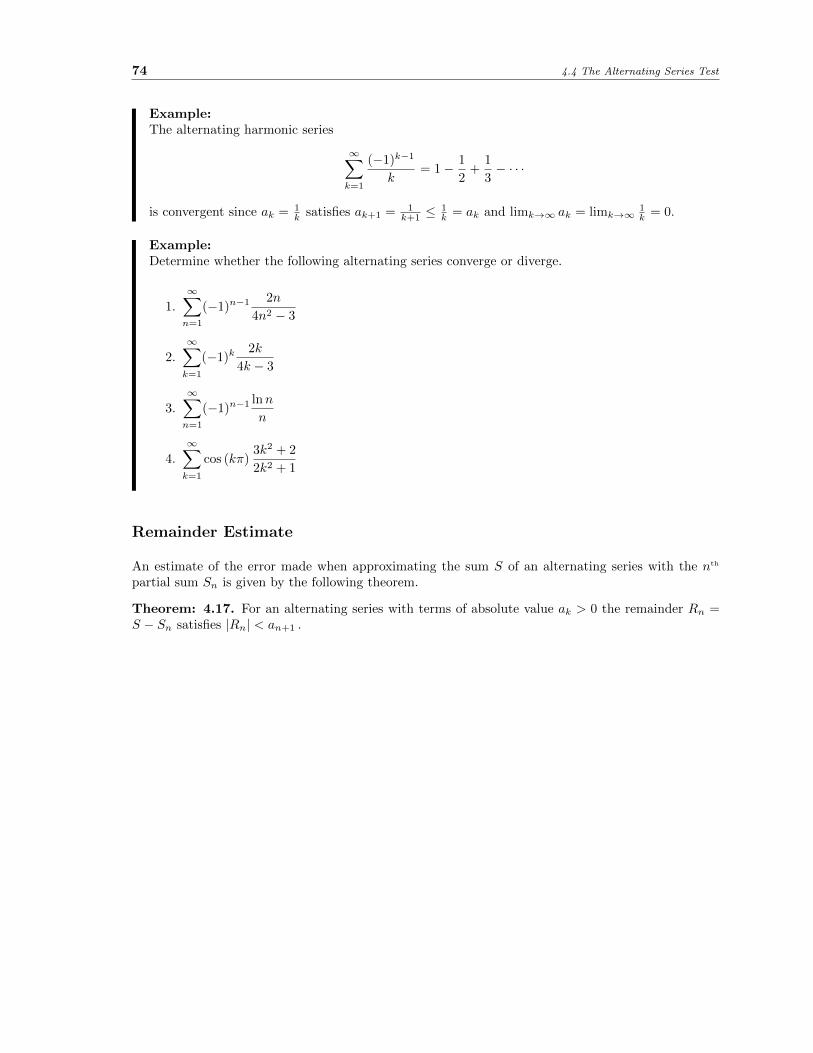
74 4.4 The Alternating Series Test
Example:The alternating harmonic series
∞∑k=1
(−1)k−1
k= 1− 1
2+
1
3− · · ·
is convergent since ak = 1k satisfies ak+1 = 1
k+1 ≤1k = ak and limk→∞ ak = limk→∞
1k = 0.
Example:Determine whether the following alternating series converge or diverge.
1.
∞∑n=1
(−1)n−12n
4n2 − 3
2.
∞∑k=1
(−1)k2k
4k − 3
3.
∞∑n=1
(−1)n−1lnn
n
4.
∞∑k=1
cos (kπ)3k2 + 2
2k2 + 1
Remainder Estimate
An estimate of the error made when approximating the sum S of an alternating series with the nth
partial sum Sn is given by the following theorem.
Theorem: 4.17. For an alternating series with terms of absolute value ak > 0 the remainder Rn =S − Sn satisfies |Rn| < an+1 .

Sequences and Series 75
4.5 Tests of Absolute Convergence
For series∑ak whose terms have mixed sign, one can consider the convergence properties of the series∑
|ak| with nonnegative terms generated by taking the absolute value of the terms of the originalseries.
4.5.1 Absolute Convergence
Definition: A series∑ak is absolutely convergent if the series
∑|ak| is convergent.
A series may be convergent that is not absolutely convergent, prompting the following definition.
Definition: A series∑ak that is convergent but not absolutely convergent is called conditionally
convergent.
Example:The alternating harmonic series 1− 1
2 + 13 −
14 + · · · is conditionally convergent because it
converges but the harmonic series, which is the sum of the absolute values of its terms, does not.
The following theorem shows a convergent series can only be absolutely or conditionally convergent.
Theorem: 4.18. If a series∑ak is absolutely convergent then it is convergent.
The theorem also shows that convergence of some series∑ak may be determined by considering
convergence of∑|ak|.
Example:Determine whether the following series are absolutely convergent or conditionally convergent.
1.
∞∑k=1
(−1)k−11
k2
2.
∞∑n=1
sinn
n2
3.
∞∑k=1
(−1)k+1 1√k
4.5.2 The Ratio Test
The following convergence test considers the limit of the ratio of terms within a series.
Theorem: 4.19. The Ratio Test:
Suppose the ratio of consecutive terms of series
∞∑k=1
ak has limit
limk→∞
∣∣∣∣ak+1
ak
∣∣∣∣ = L ,
then

76 4.5 Tests of Absolute Convergence
1. If L < 1 the series∑ak is absolutely convergent (and hence convergent).
2. If L = 1 the test is inconclusive.
3. If L > 1 the series∑ak is divergent.
If limk→∞
∣∣∣∣ak+1
ak
∣∣∣∣ =∞ then∑ak is also divergent.
Note that if the Ratio Test is inconclusive (L = 1) this means that∑ak is potentially absolutely
convergent, conditionally convergent, or divergent.
The convergence conclusions of the Ratio Test can be remembered by noting that the limit conditioneffectively suggests that the tail of the series satisfies ak+1 = Lak, in other words it behaves like ageometric series with r = L. From this it follows r = L < 1 should converge and r = L > 1 shoulddiverge.
Example:Determine whether the following series are absolutely convergent, conditionally convergent, ordivergent.
1.
∞∑k=1
(−1)k3k
k!
2.
∞∑n=1
4n
n2
3.
∞∑k=1
e−kk!
4.
∞∑n=1
2n
2n2 + 1
4.5.3 The Root Test
The next convergence test considers the limit of the kth root of |ak|.
Theorem: 4.20. The Root Test:
Suppose the terms of series
∞∑k=1
ak satisfy
limk→∞
k√|ak| = L ,
then
1. If L < 1 the series∑ak is absolutely convergent (and hence convergent).
2. If L = 1 the test is inconclusive.
3. If L > 1 the series∑ak is divergent.
If limk→∞
k√|ak| =∞ then
∑ak is also divergent.
The convergence conclusions of The Root Test can be remembered by noting that the limit conditioneffectively suggests that the tail of the series behaves like ak = Lk, in other words like a geometricseries with r = L. From this it follows that r = L < 1 should converge and r = L > 1 should diverge.

Sequences and Series 77
Example:Determine the convergence or divergence of the following series.
1.
∞∑k=1
23k+1
kk
2.
∞∑n=2
(−1)n
(lnn)n
4.5.4 Rearrangement of Series
For a finite summation of terms the order in which we add the numbers does not matter, i.e. 1+4+2 =4+1+2, or, in symbols a1 +a2 +a3 = a2 +a1 +a3. The second summation is a rearrangement of thefirst. To make the idea precise we note that the indices on the second summation, (2, 1, 3) are a per-mutation of those on the first (1, 2, 3). A permutation on the infinite set of positive indices (1, 2, 3, . . .)of a series can similarly be defined thereby making the intuitive definition of a rearrangement of aseries precise.
If a series is absolutely convergent then we get the same sum regardless of the order in which the termsare added (as expected), as summarized in the following theorem.
Theorem: 4.21. Any rearrangment of absolutely convergent series∑ak has the same sum as the
original series.
However for a series that is only conditionally convergent the order in which we add the terms doesmatter. Indeed we get the following remarkable result
Theorem: 4.22. Riemann Rearrangement Theorem: Let∑ak be a conditionally convergent
series with sum S. Then for any real number R there exists a rearrangement of series∑ak having
sum R. Additionally there exist rearrangements of series∑ak which diverge to +∞, −∞, and which
fail to approach any limit, finite or infinite.
Example:By the latter theorem it follows that the (conditionally convergent) alternating harmonic seriescan be rearranged to sum to any number or to diverge.

78 4.6 Procedure for Testing Series
4.6 Procedure for Testing Series
We have seen several methods for testing for the convergence and divergence of series. The form of theseries should suggest the type of test to be used. The following steps will be helpful for determiningconvergence and divergence of series.
1. Recognize known series with associated convergence and divergence properties:
geometric series:
∞∑k=1
ark−1 =
∞∑k=0
ark is convergent for |r| < 1 and otherwise divergent.
p-series:
∞∑k=1
1
kpis convergent for p > 1 and otherwise divergent.
(Note that p = 1 is∑
1/k the (divergent) harmonic series.)
2. If limk→∞ ak 6= 0 or that limit does not exist then the series is divergent by the Term Test forDivergence.
3. If limk→∞ ak = 0 then proceed as follows:
(a) If the terms of the series are positive, use one of the following tests.
Basic Comparison Test: Useful when ak is a rational or algebraic function of k (i.e. in-volving roots of polynomials). Consider a suitable geometric or p-series for comparison.Remember any comparison series must be positive.
Limit Comparison Test: Same criteria as the Basic Comparison Test. Choose this one ifevaluating the limit of the ratio of comparing terms is easier than proving an inequalitybetween them as required in the Basic Comparison Test.
Ratio Test: Useful for series involving factorials or other products (including a constantraised to power k). Do not use this test for rational or algebraic functions of k as theseresult in inconclusive (L = 1) results.
Root Test: Useful if ak may be written ak = (bk)k.
Integral Test: Useful if ak = f(k) for positive, continuous, decreasing f(x) and∫∞1f(x) dx
is easily evaluated.
(b) If the series is alternating (either∑
(−1)kak or∑
(−1)k−1ak for ak > 0) either:
i. Use the Alternating Series Test.
ii. Apply a positive series test from 3(a) above to the absolute value of the alternatingseries (either
∑∣∣(−1)kak∣∣ =
∑ak or
∣∣∑(−1)k−1ak∣∣ =
∑ak) since the convergence of
the latter implies the convergence of the alternating series.
(c) If the terms of the series∑ak are neither positive nor alternating, apply a test from 3(a)
above to the absolute value of the series,∑|ak|. If
∑|ak| is convergent then
∑ak is also
convergent.
(d) If the series only satisfies theorem criteria (positivity, decreasing, alternating, etc.) after acertain point (i.e. for k ≥ n for some n) apply the above steps to the tail series
∑∞k=n ak.
The convergence or divergence of the entire series will be the same as that of the tail seriessince they only differ by a finite number of terms of finite sum.

Sequences and Series 79
Examples:Determine the convergence (absolute or conditional) or divergence of the following series.
1.
∞∑k=1
2k2
k2 + 1
2.
∞∑n=1
(−1)nn
n2 + 1
3.
∞∑n=1
1000− nn!
4.
∞∑k=1
e−2k
5.
∞∑n=1
5n
n6 3n+1
6.
∞∑k=1
sin
(π
2+
1
k
)
7.
∞∑k=1
kk
10k
8.
∞∑n=1
(−1)n−1
√n
n2 + 1
9.
∞∑n=1
(1
3n+
5√n
)

80 4.7 Power Series
4.7 Power Series
We have seen that in many cases the terms of the series∑ak may be written as a function of the
summation index, namely ak = f(k), for some function f . However if the series∑ak is convergent its
value is a number, namely its sum. The final sum does not depend on the index k in the same way
that a definite integral∫ baf(t) dt results in a number independent of the dummy variable t.
Consider, however, the situation where the terms ak depend additionally on an actual variable, say x,different from the summation index, present in the series (i.e. ak = ak(x)). In this case the sum of theseries (and indeed its convergence) depends on the value of x.
Example:The geometric series with a = 1 and r = x is given by
∞∑k=0
xk = 1 + x+ x2 + · · ·+ xk + · · ·
Here ak(x) = xk. The sum is now a function of x, namely1
1− x, and is valid for |x| < 1 for which
the series is convergent.
We could introduce the variable x into the terms of a series in many ways, for instance
∞∑k=1
sin(kx)
k!.
If we choose to introduce it as in our geometric series above, namely so that the terms of the serieslook like terms in a polynomial, ckx
k, we have a power series.
Definition: Let x be a variable. A series of the form
∞∑k=0
ckxk = c0 + c1x+ c2x
2 + · · ·+ ckxk + · · · ,
where ck are real constants (for k = 0, 1, 2 . . .) is a power series in x. The constants ck arecalled the coefficients of the series.
Example:The geometric series with r = x above, 1 + x+ x2 + · · ·+ xk + · · · , is a power series in x withcoefficients ck = 1 for all k.
If we choose to make the kth term of the series have the more general form ck(x − a)k we get thefollowing.
Definition: Given real constant coefficients ck and real constant a the power series in (x− a) is
∞∑k=0
ck(x− a)k = c0 + c1(x− a) + c2(x− a)2 + · · ·+ ck(x− a)k + · · · .
The series is also known as the power series about a or centred on a.

Sequences and Series 81
A power series in x is just a special case of this last definition with a = 0.
Since the convergence of a power series (and indeed its sum should it converge) will, in general, dependon the value of the variable x, an obvious question is to find the values of x for which the power seriesis convergent.
Example:Find the values of x for which the following power series are convergent.
1.
∞∑k=0
xk
k!
2.
∞∑n=0
n2
2nxn
3.
∞∑n=1
lnn
en(x− e)n
As suggested by the previous example a power series about a will converge on an interval centred ona as detailed in the following theorem.
Theorem: 4.23. The power series
∞∑k=0
ck(x− a)k will either:
1. Converge only at x = a .
2. Converge for |x− a| < R and diverge for |x− a| > R for some positive real number R .
3. Converge for all x .
Definition: The radius of convergence R for a power series∑∞k=0 ck(x − a)k is the value R if
Part 2 of Theorem 4.23 applies. For Part 1 the radius of convergence is defined to be R = 0 andfor Part 3 the radius of convergence is defined to be R =∞.
Definition: The interval of convergence I of a power series∑∞k=0 ck(x − a)k is the set of values
of x for which the series converges. For the three possibilities of convergence one has:
1. The set containing the single value x = a (i.e. {a}) for R = 0 .
2. One of [a−R, a+R], [a−R, a+R), (a−R, a+R], or (a−R, a+R) for R > 0 finite.
3. (−∞,∞) for R =∞ .
The choice of interval in the second case depends upon the convergence or not of the series atthe interval endpoint values x = a±R .
Example:For the previous example one has the following radii and intervals of convergence:
1. R =∞, I = (−∞,∞)
2. R = 2, I = (−2, 2)
3. R = e, I = (0, 2e)

82 4.7 Power Series
Example:Find the radius and interval of convergence of each of the following series.
1.
∞∑k=0
(−1)k1
k + 1(x− 3)k
2.
∞∑n=0
n3(x− 5)n
3.
∞∑k=0
k!(2x− 1)k
4.
∞∑n=1
(2x− 3)n
n 3n

Sequences and Series 83
4.8 Representing Functions with Power Series
The sum of a power series for a given x from its interval of convergence I results in a number. As suchit is natural to consider the power series as defining a function f(x) of x on I with the value of thefunction being the sum. We write
f(x) =
∞∑k=0
ckxk (x ∈ I)
If the sum of the power series can be written in a closed form, then the power series can be considereda representation of that function valid on I.
Example:The power series
∑∞k=0 x
k = 1 + x+ x2 + · · · converges for |x| < 1, and therefore is a function of xon I = (−1, 1). On that interval the sum for given x is 1
1−x . The power series thus is a
representation of the function 11−x on this restricted domain:
1
1− x= 1 + x+ x2 + · · ·+ xk + · · · =
∞∑k=0
xk for |x| < 1
One can find power series representations of other functions using known power series.
Example:Find representations of the following functions with power series. Indicate the values of x forwhich the representations are valid.
1.1
1 + x
2.1
1− x3
3.x
2− 3x
As functions power series behave like polynomials. They are continuous and can be termwise differen-tiated and integrated to produce new functions of x as detailed in the following theorem.
Theorem: 4.24. Suppose f(x) is defined by the power series
f(x) =
∞∑k=0
ck(x− a)k = c0 + c1(x− a) + c2(x− a)2 + · · ·+ ck(x− a)k + · · ·
with radius of convergence R > 0 (finite or infinite). Then on the interval (a−R, a+R) :
1. f(x) is continuous.
2. f(x) is differentiable with derivative
f ′(x) =
∞∑k=0
kck(x− a)k−1 = c1 + 2c2(x− a) + 3c3(x− a)2 + · · ·+ kck(x− a)k−1 + · · ·

84 4.8 Representing Functions with Power Series
3. f(x) is integrable with integral∫f(x) dx = C+
∞∑k=0
ckk + 1
(x−a)k+1 = C+c0(x−a)+c12
(x−a)2+c23
(x−a)3+· · ·+ ckk + 1
(x−a)k+1+· · ·
The series resulting from differentiation and integration both have radius of convergence R .
Note that the above theorem shows that for power series the calculus operations of differentiation andintegration can be exchanged with summation, just as occurs with finite sums.
d
dx
∑ck(x− a)k =
∑ d
dx
[ck(x− a)k
]∫ [∑
ck(x− a)k]dx =
∑[∫ck(x− a)k dx
]If the power series is a representation of a function with a closed form, differentiation and integrationcan be used to find power series representations of other functions.
Example:Find a power series representation for each of the following functions. Indicate the interval forwhich the representation is valid.
1.1
(1 + x)2
2. ln(1 + x)
3. tan−1x
Because power series representations are easy to integrate, they may be used as a means to integratedifficult functions. The integral will only be valid for x lying within (a−R, a+R).
Example:Integrate each of the following using a power series.
1.
∫1
1 + x3dx
2.
∫x
1− x4dx

Sequences and Series 85
4.9 Maclaurin Series
We expect some functions f(x) can be represented by an infinite series∑∞k=0 ckx
k for a certain,potentially restricted, domain. While we verified that 1
1−x could be represented by the geometricseries, we would like a general mechanism for determining the coefficients of the power series thatcorrespond to an arbitrary f(x). Suppose f(x) has a power series expansion:
f(x) = c0 + c1x+ c2x2 + c3x
3 + c4x4 + · · · .
One observes that if we set x = 0 that f(0) = c0. In other words, we can determine c0 by evaluatingf at x = 0. We can differentiate the power series above term by term to get:
f ′(x) = c1 + 2c2x+ 3c3x2 + 4c4x
3 + · · ·
If we evaluate this at x = 0 we get c1 = f ′(0). The next derivative is:
f ′′(x) = 2c2 + 6c3x+ 12c4x2 + · · ·
and so c2 = f ′′(0)2 . Repeated differentiation and evaluation relates the kth coefficient ck to the derivative
f (k) evaluated at x = 0 as follows:
ck =f (k)(0)
k!
where recall the factorial is defined by k! = k · (k− 1)· · ·2 · 1. The formula is true for k = 0 as wellwith the convention f (0)(x) = f(x) and noting that 0! = 1 by definition. Plugging our ck into theoriginal power series we get the following definition.
Definition: Given function f(x) differentiable to all orders at x = 0 the power series in x given by
f(x) =
∞∑k=0
f (k)(0)
k!xk = f(0) + f ′(0)x+
f ′′(0)
2!x2 +
f ′′′(0)
3!x3 + · · · f
(k)(0)
k!xk + · · ·
is the Maclaurin series for f(x).
As a power series, the Maclaurin series must converge for |x| < R for some radius of convergence Rdependent upon the function.4
Examples:Find the Maclaurin series and its interval of convergence for each of the following functions.
1. f(x) =1
1− x
2. f(x) = ex
3. f(x) = sinx
4. f(x) = ln(1 + x)
4We will discuss shortly whether the Maclaurin series of f(x) actually is a valid representation of the function onthis interval.

86 4.9 Maclaurin Series
Some important Maclaurin series and their domains of validity are:
1
1− x=
∞∑k=0
xk = 1 + x+ x2 + x3 + · · · ; (−1, 1)
ex =
∞∑k=0
xk
k!= 1 +
x
1!+x2
2!+x3
3!+ · · · ; (−∞,∞)
sinx =
∞∑k=0
(−1)kx2k+1
(2k + 1)!= x− x3
3!+x5
5!− x7
7!+ · · · ; (−∞,∞)
cosx =
∞∑k=0
(−1)kx2k
(2k)!= 1− x2
2!+x4
4!− x6
6!+ · · · ; (−∞,∞)
tan−1 x =
∞∑k=0
x2k+1
2k + 1= x− x3
3+x5
5− x7
7+ · · · ; [−1, 1]
ln(1 + x) =
∞∑k=0
(−1)kxk+1
k + 1= x− x2
2+x3
3− x4
4+ · · · ; (−1, 1]
As we saw with the more general power series, we can derive series of new functions from knownMaclaurin series.
Example:For the following functions we have the power series:
1. ex3
=
∞∑k=0
(x3)k
k!=
∞∑k=0
x3k
k!
Series is valid for x3 in (−∞,∞) which implies for x in (−∞,∞).
2. sin2x =1
2(1− cos 2x) =
1
2− 1
2
∞∑k=0
(−1)k(2x)2k
(2k)!=
1
2+
∞∑k=0
(−1)k+1 22k−1x2k
(2k)!
Series is valid for 2x in (−∞,∞) and so for x in (−∞,∞).
These series can be confirmed to be the Maclaurin series of the given functions by directcomputation.

Sequences and Series 87
4.10 Taylor Series
Maclaurin series can be generalized by expanding in powers of (x − a)k rather than xk for someconstant a. A similar argument to that before gives the following definition.
Definition: Given function f(x) differentiable to all orders at x = a the power series in (x− a) givenby
f(x) =
∞∑k=0
f (k)(a)
k!(x−a)k = f(a)+f ′(a)(x−a)+
f ′′(a)
2!(x−a)2+
f ′′′(a)
3!(x−a)3+· · · f
(k)(a)
k!(x−a)k+· · ·
is the Taylor Series for the function f(x) at a (or about a or centred on a).
The Taylor series expansion at a will converge within some radius R about a, i.e. for |x− a| < R.
We note that Maclaurin series is just a special case of the Taylor series when a = 0.
Examples:Find the Taylor Series of the given function at the specified value and determine the interval ofconvergence.
1. f(x) = sinx at a =π
2
2. f(x) = lnx at a = 1
3. f(x) = ex at a = 2
Assuming convergence to f(x), Taylor series gives us a mechanism for calculating trigonometric andother functions, namely by evaluating the first n terms of the series at x. How many terms of theseries are required for a good approximation will depend on the function, the value a about which itis expanded, and x.
Tayor series allows expansion of the function f about values other than a = 0 which is useful forfunctions that are not defined at 0. Also in general fewer terms of the expansion will be required fora good approximation if the Taylor series is generated about a value a near the x of interest. Indeedby truncating the Taylor series at the k = 1 term
f(x) ≈ f(a) + f ′(a)(x− a) ,
or at the k = 2 term,
f(x) ≈ f(a) + f ′(a)(x− a) +f ′′(a)
2!(x− a)2 ,
we are just reproducing the linear and quadratic approximations of a function at x = a arrived at ourprevious course. In general truncating at the k = nth term,
f(x) ≈ f(a) + f ′(a)(x− a) +f ′′(a)
2!(x− a)2 +
f ′′′(a)
3!(x− a)3 + · · ·+ f (n)(a)
n!(x− a)n
yields increasingly better approximations. The right hand side is called the nth Taylor polynomialof the function f(x) at a. The following diagram shows the first four Taylor polynomials of sinx ata = 0 (i.e. the Maclaurin series):

88 4.10 Taylor Series
y
x
y = sin(x)
n = 1
n = 3
n = 5
n = 7
Taylor polynomials (a = 0)
Here are the first four polynomials for the Taylor series of sinx at a = π/2:
y
x
y = sin(x)
n = 0
n = 2
n = 4
n = 6
π2
Taylor polynomials (a = π/2)
One observes both the greater accuracy of the higher order approximations as well as the utility ofexpanding the Taylor series at a value a near the x at which you wish to approximate the function.
One useful result of Theorem 4.24 is that it justifies our original proof for the coefficients for theMaclaurin series where (recall) we required the power series to be differentiable. Generalizing thisresult to Taylor series we have the following result:
Theorem: 4.25. If function f(x) is represented by the power series
f(x) =
∞∑k=0
ck(x− a)k = c0 + c1(x− a) + c2(x− a)2 + · · ·
on an open interval containing a then the coefficients are the Taylor series coefficients ck = f (k)(a)/k!,
(i.e. f(x) = f(a) + f ′(a)(x− a) + f ′′(a)2! (x− a)2 + · · · ).
In other words, if a function f(x) has a power series that converges to f(x) it will be the Taylor series.The theorem does not say, however, that the Taylor series at a for a given function f will necessarily

Sequences and Series 89
converge to f . For instance define the continuous piecewise function:
f(x) =
0 if x < −π/2cosx if −π/2 ≤ x ≤ π/2
0 if x > π/2
Then f will have the same Taylor series at a = 0 (i.e. Maclaurin series) as the function cosx. Howeverthat series clearly cannot represent both functions. One must determine that the Taylor series for fat a really does converge to the function.
Theorem: 4.26. If a function f has derivatives to all orders in an interval centred on a, then
f(x) =
∞∑k=0
f (k)(a)
k!(x− a)k
will hold on the interval if and only iflimn→∞
Rn(x) = 0
for all x in the interval, where
Rn(x) = f(x)−n∑k=0
f (k)(a)
k!(x− a)k .

90

Unit 5: Integration Applications
91

92 5.1 Areas Between Curves
5.1 Areas Between Curves
We have already seen this topic in a previous course. We review it here for the purpose of remindingourselves how to interpret differentials in integration formulae.
We have already calculated an area between curves. Namely, when y = f(x) ≥ 0 on [a, b] then
A =
∫ b
a
f(x) dx
is the area below the curve y = f(x) and above the x-axis. But since the y-axis is just the curve y = 0,the above integral is also the area between the curve y = f(x) and the curve y = 0. If the lower curveis y = g(x) instead of y = 0 we get the following result:
Theorem: 5.1. If y = f(x) and y = g(x) are integrable on the x-interval [a, b] with f(x) ≥ g(x) onthe interval then the area between the curves y = f(x) and y = g(x) and the lines x = a and x = bis
A =
∫ b
a
[f(x)− g(x)] dx .
The situation is illustrated in the following diagram:
y
xx = a x = b
A
y = f(x)
y = g(x)
dx
f(x)− g(x)
dA
A simple way to remember the theorem is the differential notation. We are finding the sum A =∫dA
of the infinitesimal rectangle areas each of area dA where
dA = [f(x)− g(x)]︸ ︷︷ ︸height
· dx︸︷︷︸width
.
Sometimes the region for which one wants an area is better described by functions x = f(y) andx = g(y) denoting the right and left boundaries of the region respectively. One then has the result:
Theorem: 5.2. If x = f(y) and x = g(y) are integrable on the y-interval [c, d] with f(y) ≥ g(y) onthe interval then the area between the curves x = f(y) and x = g(y) and the lines y = c and y = dis
A =
∫ d
c
[f(y)− g(y)] dy .

Integration Applications 93
The situation is depicted below:
x
y
y = c
y = d
A
x = f(y)x = g(y)
dyf(y)− g(y)
dA
In this case the integral represents the addition of horizontal area elements dA of area
dA = [f(y)− g(y)]︸ ︷︷ ︸width
· dy︸︷︷︸height
.
Sometimes no interval [a, b] or [c, d] is given. If one is asked to find the region bounded by y = h1(x) andy = h2(x) one uses vertical area elements (first theorem) to find the area. One must solve h1(x) = h2(x)to find x-values xi which enclose the bounded region(s). There may be multiple enclosed regions andthese values determine the endpoints of the integration. One must ascertain which function is thehigher one on each region.
If one is asked to find the region bounded by x = h1(y) and x = h2(y) then one uses horizontal areaelements (second theorem) to find the area. One must solve h1(y) = h2(y) to find y-values yi whichenclose the bounded region(s). Once again these determine the endpoints of integration. One mustdetermine which function is greater on each region.
Examples:Find the area of the region bounded by the following curves:
1. y = 6− x2 and y = 3− 2x
2. x = y2 and x− y − 2 = 0

94 5.2 Calculation of Volume
5.2 Calculation of Volume
5.2.1 Volume as a Calculus Problem
The volume of a three-dimensional object is the amount of space it occupies (expressed in cubicunits). If we had an odd-shaped jar and had a bag of caramels that were a cm on each side we couldestimate the jar’s volume by counting the number of caramels that would fit in the jar. This wouldbe the volume in cubic centimetres (i.e. millilitres). In a more accurate estimate we would fill the jarwith water and then measure the number of millilitres with a measuring cup.
We are interested in how we can use calculus to find such volumes. An object for which we have aformula for volume is a right cylinder. A cylinder is a three-dimensional geometric figure that hastwo congruent and parallel bases. When the bases are aligned one directly above the other one has aright cylinder. The following are three examples of right cylinders:
AAA
hh h
V = Ah = πr2h
wr
V = Ah = lwhV = Ah
l
The first shows the most general case, while the second and third are special cases, a rectangularparallelepiped and a right circular cylinder, respectively. In general the area of a right cylinder is:
V = Ah
In the special case where the area is expressible in terms of other lengths we can further specialize theformula. So a right circular cylinder has volume:
V = πr2h
Returning to the general case of finding a volume of an arbitrary 3D object we may follow the sameroute we did for solving general areas. In the area case we sliced the figure into increasingly thinnerrectangles (∆x→ 0) and then added those up. For a 3D object we can imagine slicing it into a largenumber of increasingly thinner (shorter) right cylinders (of height ∆h → 0) and adding them up. Todo this we take an abitrary axis through our solid S and partition the axis into equal widths ∆h. Ateach point h along the axis we will have a cross-sectional area A in the plane perpendicular to ouraxis h.

Integration Applications 95
������������������������������������������������������������������������
������������������������������������������������������������������������
dh
h
AS
The area A will depend upon the position h along the axis and so it is a function A(h) of h. Thevolume of our object will then be the limit of the Riemann Sum of the n cylinders with volumes Vi:
V = limn→∞
n∑i=1
A(h∗i )∆h︸ ︷︷ ︸Vi
The position h∗i is taken to be a point in the corresponding interval along h of the ith cylinder. Thislimit is the definite integral:
V =
∫ b
a
A(h)dh ,
where a and b denote the position of the first and last cylinders needed. Thinking in differentialnotation we are summing (
∫dV ) the volumes of infinitessimally thin cylinders given by:
dV = Adh
5.2.2 Solids of Revolution
In general the function A(h) for a particular solid S will be complicated. However if the solid has asymmetry and the axis h is directly along that axis of symmetry the function A(h) may be calculated. Acertain class of solids, called Solids of Revolution have such a symmetry because they are generatedby sweeping out a two dimensional area around just such an axis:

96 5.2 Calculation of Volume
Sphere Cone
Semicircle Triangle
Vase (?)
Solids of Revolution
y=f(x)
As can be seen in the diagram some common shapes (spheres and cones) can be thought of as solidsof revolution of simple areas (semicircles and triangles). Other interesting shapes may be constructedby choosing other functions for the upper boundary.
5.2.3 The Disk Method
For a solid of revolution for which the planar area of the revolution extends from the axis of symmetryto a boundary curve describable by a function, the volume is now calculable because the area functionA(h) can be found:
Disk Method
dV = πr2dh
r
h
r
dh
r = f (h)
ba
As shown in the diagram, the general right cylinders are now right circular cylinders with areaA = πr2. Our volume element is the disk of differential volume:
dV = πr2dh

Integration Applications 97
where the radius r for the given disk is r = f(h). The volume is then the sum (V =∫dV ) given by
V =
∫ b
a
πr2 dh =
∫ b
a
π [f(h)]2dh
If the symmetry axis is the x-axis (so h = x and r = y = f(x)) then the formula for a solid of revolutionabout the x-axis becomes
V =
∫ b
a
π [f(x)]2dx
This method of calculating volumes is called the Disk Method because we are approximating thevolume with disks (i.e. short right cylinders).
Example:Find the volume of the solid obtained by revolving the following regions about the x-axis:
� The region bounded by the curves y = x32 , x = 4 and y = 0.
� The region bounded by the curve y = 2x− x2 and the line y = 0.
The constant π is defined to be the ratio of the circumferance to the diameter of any circle, π = Cd .
Archimedes (c. 287-212 BCE) discovered (long before the invention of calculus) that the constant πsurprisingly shows up in the formulas for the area of a circle (A = πR2) as well as for a sphere’s volume(V = 4
3πR3) and surface area (S = 4πR2).
Example:Use calculus to show the volume of a sphere of radius R is V = 4
3πR3.
We sometimes wish to revolve a region about the y-axis. For a region bounded by the curve x = f(y)and the lines x = 0 (i.e. the y-axis), y = c, and y = d we can use horizontal disks. In this case dh = dy(since the symmetry axis h is now y) and r = x = f(y) as shown in the following diagram.
y
d
x = f (y)
dy
x
c
x(x, y)
The formula for the volume of such a region revolved about the y-axis is therefore:
V =
∫ d
c
π [f(y)]2dy

98 5.2 Calculation of Volume
Example:Find the volume of revolution of the solid obtained by revolving the region bounded by y = x2,x = 0, and y = 4 about the y-axis.
In general we may be interested in revolving an area about a horizontal or vertical axis which isneither the x nor the y-axis. In this case we must work from the differential volume dV to determinethe volume integral. Follow the following steps which will work for any volume problem:
1. Draw the region to be revolved labelling the curves appropriately as well as points of intersection.Draw the symmetry line about which the curve is to be revolved.
2. Decide on the differential volume element you will use and indicate a typical cross-section rect-angle on your region.
3. Label the endpoints of rectangle with coordinates (x, y), etc. Note that for vertical elements theendpoint coordinates will have the same endpoint x values while you will need to distinguish they values (i.e. y1, y2) as these values will differ. If a value is constant (e.g. 0) for all potentialcross-section rectangles label it as such instead of using a variable. The opposite holds if you areusing a horizontal element (i.e. same y values at endpoints, different x’s.)
4. Label the differential width of the cross-section rectangle as dx or dy according to whether youare using a vertical or horizontal elements respectively.
5. Write down your integral, V =∫dV , and substitute your volume element for dV .
6. Next replace each variable in the integral in terms of the variables of your cross-section rectangleendpoint coordinate variables. Some calculation may be required here, especially if you are notrevolving about a coordinate axis.
7. From your diagram determine the limits of integration. These must be along the same axis asfound in your differential, i.e. x for dx or y for dy. Note the limits are for the rectangles onlywithin the region being revolved.
8. All variables of the integrand must be in terms of the integration variable. Replace any variablesin your integral that are not the same as the differential variable in terms of the differentialvariable by considering the curve that the endpoint involving the variable lies upon. You mayneed to solve for the variable using the curve equation to do so.
9. Calculate the integral.
Example:Find the volume of the solid generated by revolving the region bounded by y = x2 and y = 4about the line y = 4.
5.2.4 The Washer Method
Suppose we generate a solid of revolution in which the lower boundary is not the axis of revolutionbut, more generally the curve g(h) above it. These regions are what we considered when we lookedat areas between curves having an upper boundary determined by a function f and a lower boundarydetermined by a function g. If such a region is revolved about a chosen axis of symmetry h then thesolid of revolution generated will have a hole in it and the disk method will not, at first glance, work.
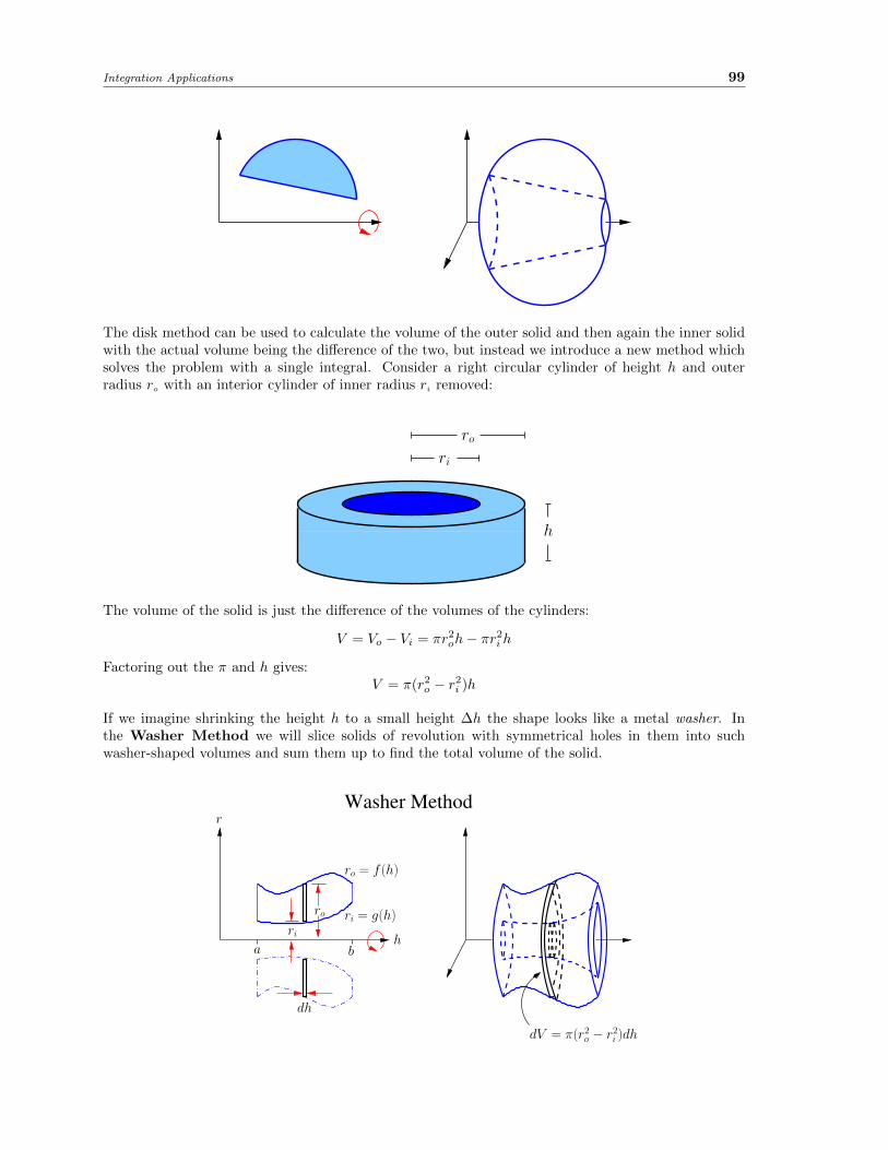
Integration Applications 99
The disk method can be used to calculate the volume of the outer solid and then again the inner solidwith the actual volume being the difference of the two, but instead we introduce a new method whichsolves the problem with a single integral. Consider a right circular cylinder of height h and outerradius ro with an interior cylinder of inner radius ri removed:
h
ri
ro
The volume of the solid is just the difference of the volumes of the cylinders:
V = Vo − Vi = πr2oh− πr2i h
Factoring out the π and h gives:V = π(r2o − r2i )h
If we imagine shrinking the height h to a small height ∆h the shape looks like a metal washer. Inthe Washer Method we will slice solids of revolution with symmetrical holes in them into suchwasher-shaped volumes and sum them up to find the total volume of the solid.
Washer Method
dV = π(r2o − r2
i )dh
h
r
dh
ba
ri
ro
ro = f (h)
ri = g(h)

100 5.2 Calculation of Volume
In the Washer Method the height of the washer ∆h is replaced with the differential dh so the differentialelement of volume is:
dV = π(r2o − r2i )dh
The total volume is just the sum (V =∫dV ) and we have:
V =
∫ b
a
π(r2o − r2i )dh =
∫ b
a
π([f(h)]2 − [g(h)]2
)dh
where we have replaced the outer and inner radii by their functional values at h (see diagram). If thesymmetry axis is the x-axis (so h = x, ro = y2 = f(x), and ri = y1 = g(x)) then the formula for asolid of revolution about the x-axis becomes
V =
∫ b
a
π([f(x)]2 − [g(x)]2
)dx
This may always be found starting with the differential volume element dV = π(r2o − r2i )dh andfollowing the general steps.
Example:Find the volume of the solid obtained by revolving the region bounded by the curves y = x2 + 1and y = 3− x2 about the x-axis
If the symmetry axis is the y-axis then h = y and we can write the outer radii as ro = x2 = f(y)and the inner radii as ri = x1 = g(y). The general formula for a solid of revolution about the y-axisbecomes:
V =
∫ d
c
π([f(y)]2 − [g(y)]2
)dy
Once again we use our convention of using constants c and d for limits along the y-axis.
Example:Find the volume of the solid obtained by revolving the region bounded by y = 2x and y = x2
about the y-axis.
If one is revolving about an axis that is not a coordinate axis there is no immediate formula since thecurve functions no longer represent distances from the axes of revolution. Follow the steps outlinedpreviously starting with the volume element and identifying the variables from your diagram. In thiscase the radii will need to be calculated in terms of the variables.
Example:Find the volume of the solid obtained by revolving the region bounded by the curves y = 3
√x and
y = 14x and lying in the first quadrant (x ≥ 0 and y ≥ 0) about the line x = 10.

Integration Applications 101
5.3 The Shell Method
Suppose one wished to calculate the volume of the solid generated by revolving the region bounded bythe curve y = sin(x2) and the line y = 0 about the y-axis as shown.
y
√π
y = sin(x2)
0x
While one can imagine dividing the solid into washer-shaped regiond perpendicular to the y-axis, therewould be difficulties.
y
√π0
x
y = sin(x2)
x = g(y) x = f(y)
Ultimately we would need to solve for x in terms of y to find the inner and outer radii of the washerin terms of the position y of the disk. This could be tricky in part because of the trigonometricfunction. Moreover in inverting the function we would somehow need to generate both an upper andlower function x(y) corresponding to the two radii of the washer!
We now consider a different approach by the introduction of a new volume element. Recall the cylinderwith the inner cylinder removed.
h
ri
ro

102 5.3 The Shell Method
We found before the formula for the volume of this solid was just the difference of the volume of thecylinders:
V = π(r2o − r2i
)h
Notice that we can factor the difference of squares:
V = π (ro + ri) (ro − ri)h
Defining the average radius r to be:
r =ro + ri
2,
and the difference of the radii to be∆r = ro − ri ,
we can rewrite the volume asV = π(2r)(∆r)h ,
or equivalentlyV = 2πrh∆r .
Now suppose we make the two radii approximately equal. Then the average radius r approximatelyequals either of them with little error, while their difference ∆r will be small. The solid will be like acylindrical tin can (with the ends cut off) which we will refer to as a “shell”. The volume formula forthe shell now becomes quite intuitive. If we imagine cutting the shell along its length and unrolling itwe would effectively have a rectangular sheet with top length equalling the circumference of the circle(2πr) and the other side length equalling the height. The thin thickness will be ∆r.
2πr
∆r
h
∆r r
cut
her
e
So the volume of the rectangular sheet (the shell) is then:
V = (circumference)(height)(depth) = (2πr)(h)(∆r) = 2πrh∆r
as found before.
Now in the Shell Method we imagine slicing the solid of revolution into concentric cylindrical shellsand adding up the volumes.
Shell Method
dV = 2πrh dr
dra
h
hr
b
h = f (r)
r

Integration Applications 103
In the limit that the number of shells goes to infinity, so ∆r → 0, the limit of the Riemann Sum is anintegral (
∫dV ) of differential volume
dV = 2πrh dr
with, as usual the finite V and ∆r replaced with dV and dr in our shell volume formula. Specifically,for the region depicted above we have for the volume of the solid of revolution
V =
∫ b
a
2πrh dr =
∫ b
a
2πrf(r) dr
Notice that in the Shell Method the differential dr is now perpendicular to the axis of symmetry.
If the axis of symmetry is the y-axis then, setting h = y and r = x in the above formula we get thefollowing result for an a solid of revolution generated by revolving the region bounded by the curvey = f(x), y = 0, x = a, and x = b about the y-axis:
V =
∫ b
a
2πxf(x) dx
Example:Find the volume of the solid generated by revolving the region bounded by the curves y = sin(x2)and y = 0 between x = 0 and x =
√π about the y-axis.
If the axis of symmetry is the x-axis then, setting h = x and r = y in the above formula we get thefollowing formula for a solid of revolution generated by the region bounded by the curves x = f(y),x = 0, y = c, and y = d.
V =
∫ d
c
2πyf(y) dy
More generally the lower bound of the region need not be along the radial axis:
h
bar
h = g(r)
h = f (r)
If the upper bound of the figure remains described by the function h = f(r) while the lower boundis now the function h = g(r) the the height of the shell is h = f(r) − g(r). The volume for the solidgenerated by revolving about the h-axis is then
V =
∫ b
a
2πrh dr =
∫ b
a
2πr [f(r)− g(r)] dr

104 5.3 The Shell Method
One observes that, in the example depicted, the washer method would now be impossible in a singleintegral. For even should we be able to solve for r(h) on the curves, there is no single washer generatedtoward the bottom of the region. One also notes in this example that the region is generally boundedby four curves, two are vertical lines. In general the shell method works well for solids with straightcylindrical boundaries parallel to the axis of revolution.
In the event we are revolving about the y-axis, so h = y and r = x in the above diagram, the solidgenerated by revolving the region bounded by y = f(x), y = g(x), x = a and x = b is
V =
∫ b
a
2πx [f(x)− g(x)] dx
On the other hand the volume of the solid generated by revolving about the x-axis the region boundedby x = f(y), x = g(y), and the horizontal lines y = c and y = d is, setting h = x, and r = y,
V =
∫ d
c
2πy [f(y)− g(y)] dy
These formulae may all, as usual be derived following the general steps starting with the differentialvolume element dV = 2πrh dr.
Example:Find the volume of the solid generated by revolving the region bounded by the curves x2 = 4y andy = 4 about the x-axis.
If one wishes to use the shell method to evaluate a solid generated by revolution of a region about anon-coordinate axis the differential volume element dV = 2πrh dh and the general steps must be used.
Example:Find the volume of the solid generated by revolving the region bounded by the curves y = x2 andx+ y = 2 about the line x = 3.

Integration Applications 105
5.4 Determining the Volume Method
We have considered several methods for calculating volumes of solids of revolution. Which to use in aparticular instance can be determined by the following set of steps:
1. Draw the region to be revolved and identify the axis of revolution.
2. Next imagine a line perpendicular to the axis of revolution. Where this intersects the regionrepresents (the cross-section of) a particular volume element. Slide the line through the regionkeeping it perpendicular to the axis of revolution. If all such lines intersect the boundary of theregion two or fewer times then the Disk/Washer Method will potentially work. An exceptionto the intersection rule is when you first enter and leave the region; here one can intersect theboundary in a straight line.
As you pass the line through the region consider the endpoints of the intersection with the region.If these do not always lie on the same curves then the region will need to be partitioned into two(or more) regions each requiring a separate integral to use this method.
3. Repeat the previous step but now with lines parallel to the axis of revolution. If the region passesthis test then it is a candidate for the Shell Method.
4. For any region that passes the Disk/Washer test, if one of the boundary curves of the region isthe axis of revolution then use the Disk Method for that interval, otherwise the Washer Methodwill be used.
5. To distinguish multiple candidate methods, next look at the curve equations. Identify the variableof integration (dx or dy). It will be the variable of the coordinate axis parallel to the axis ofrevolution in the case of the Disk/Washer Method and perpendicular to the axis of revolutionfor the Shell Method. The curves in the boundary region (aside from any straight lines at thebeginning or end of the region for the method in question) will have to have the non-differentialvariable written as a function of the differential variable. If these curves cannot be solved for thenon-differential variable, reject the method.
6. If several candidate methods still remain, set up the volume integral for one candidate. If it isnot easily solved, try the other candidate.
7. If no candidates lead to a solution, then the solid cannot be calculated with a single volumemethod. Try partitioning the region into several areas and calculate the volume for each regionrevolved separately. If these can be calculated the volume of the entire solid is their sum.

106 5.4 Determining the Volume Method
Example:For each of the following regions identify the simplest volume method(s) to use to calculate thesolid of revolution found by rotating the region about the indicated axis. For the method statewhether to use vertical or horizontal differential volume elements.
a) b) c)
e) f)d)
x
y
x
y
x
y
x
y
x
y
x
y

Integration Applications 107
5.5 Arc Length
From basic geometry the perimeter P of a polygon or the circumference C of a circle are the distancearound the given object. They are the length one would measure if the boundary of the object werecut, straightened out, and measured with a ruler.
x
y
r
C = 2πrP = 2x + 2y
Intuitively the arc length s of a curve between points P and Q is similarly the “length of a piece ofstring” that follows the curve joining those two points.
y
x
sP
Q
y = f(x)
a b
Consider a curve defined by a function y = f(x) with a continuous first derivative f ′(x) definedon interval [a, b]. Such a function is called a smooth function and its graph y = f(x) is said to besmooth. An approximation to the arc length can be found by breaking the interval into n subintervalsof equal length ∆x = b−a
n with endpoints
a = x0, x1, x2, . . . , xn−1, xn = b
The points Pk = (xk, f(xk)), k = 0, 1, . . . , n, lie along the curve. The length of the chord (straight linesegment) joining Pk−1 to its neighbour Pk will approximate the arc length between those two points.Call that chord length ∆sk. It equals, by the Pythagorean Theorem, ∆sk =
√(∆x)2 + (∆yk)2 where
we define ∆yk = yk − yk−1 = f(xk)− f(xk−1).

108 5.5 Arc Length
y
x
y = f(x)
a = x0 x1 xk−1 xk xn = b
Pk−1
Pk
∆x
∆yk
∆sk
By the Mean Value Theorem applied to the interval [xk−1, xk] there exists an x∗k in (xk−1, xk) satisfying
f(xk)− f(xk−1)
xk − xk−1= f ′(x∗k)
Equivalently ∆yk = f ′(x∗k)∆x. From this it follows that we can write ∆sk as:
∆sk =√
(∆x)2 + (∆yk)2
=
√(∆x)2 + [f ′(x∗k)∆x]
2
=
√(∆x)2 + [f ′(x∗k)]
2(∆x)2
=
√(1 + [f ′(x∗k)]
2)· (∆x)2
=
√1 + [f ′(x∗k)]
2 ·√
(∆x)2
=
√1 + [f ′(x∗k)]
2∆x
An approximation to the arc length between the points P (a, f(a)) and Q(b, f(b)) is therefore the lengthof the polygonal curve we have constructed, namely the Riemann sum
n∑k=1
∆sk =
n∑k=1
√1 + [f ′(x∗k)]
2∆x
Taking the limit as n→∞ (so ∆x→ 0) we have the following:
Definition: If function f has a continuous derivative f ′ over the x-interval [a, b] then the length ofthe graph over the interval (the arc length) is
s =
∫ b
a
√1 + [f ′(x)]2 dx or s =
∫ b
a
√1 +
(dy
dx
)2
dx
Note that if a curve is described by the equation x = g(y) with continuous derivative g′(y) over they-interval [c, d] then the arc length between the endpoints equals
s =
∫ d
c
√1 + [g′(y)]2 dy or s =
∫ d
c
√1 +
(dx
dy
)2
dy

Integration Applications 109
Examples:Find the lengths of the following curves over the given intervals.
1. f(x) = 3x23 − 10 over 8 ≤ x ≤ 27
2. y =x4
16+
1
2x2over 1 ≤ x ≤ 2
If we have a smooth function f(x) on interval [a, b] we can consider the arc length from the startingpoint (a, f(a)) up to the point (x, f(x)) for some value x in [a, b]. This length is clearly dependent onthe choice of x and hence is a function s(x).
Definition: Given a smooth curve described by the function y = f(x) over the x-interval [a, b], thearc length between the initial point (a, f(a)) and the point (x, f(x)) for x in [a, b] is given by thearc length function
s(x) =
∫ x
a
√1 + [f ′(t)]2 dt
Notes:
1. We changed the variable of integration to t to distinguish it from the limit of integration x.
2. The derivative of the arc length function s(x) is, by the Fundamental Theorem of Calculus,dsdx =
√1 + [f ′(x)]2 . This in turn implies, since ds = ds
dx dx, that the differential of the arclength is
ds =√
1 + [f ′(x)]2dx .
Noting that dy = f ′(x)dx the differential of arc length is sometimes written
ds =√dx2 + dy2 ,
reflecting its Pythagorean origins. The latter differential formula, along with the relation dy =f ′(x)dx for x-intervals [a, b] or dx = g′(y)dy for y-intervals [c, d], and the idea of the integral asa sum (s =
∫ds) make it easy to remember/derive the arc length formulae.
Examples:Find the arc length function s(x) of
1. y =√x− x2 − cos−1
(√x)
with starting point P (0,−π/2).
2. y = ex with starting point P (0, 1).

110 5.6 Areas of Surfaces of Revolution
5.6 Areas of Surfaces of Revolution
Just as volumes of revolution are constructed by revolving an area about a line, a surface of revo-lution is generated by revolving the graph of a continuous function about a line.
Sphere Cone
Semicircle
Surfaces of Revolution
Frustum of a Cone
LineLine
Note that the surface generated in this manner does not produce any end surfaces such as the cir-cular bottom of the cone or ends of the frustum of the cone. (The spherical surface however is fullygenerated.)
We turn ourselves to the problem of calculating the area of such a surface of revolution. Consider asimple object like the frustum of the cone above, with end radii of r1 and r2 and slant height s.
r2
r1
s
The lateral surface area of the frustum (i.e. the area of the side but not including the circular ends),can be shown to be
S = 2πrs ,
where r = 12 (r1 + r2) is the average of the two radii.
The approximate area of a surface of revolution may be found by slicing it perpendicular to its axis ofrevolution (which we will call h). The intersection of these planes with the surface form the circular

Integration Applications 111
ends of conical frusta the net lateral surface area of which will approximate the area of the surface ofrevolution.
Differential Surface Area
dS = 2πr ds
h
r
r
ds
A Riemann sum for the area is thereby formed:
S ≈n∑k=1
∆Sk ,
where ∆Sk is the lateral surface area of the kth conical frustum. Upon taking the limit of an infinitenumber (n → ∞) of conical frusta one arrives at an exact expression for the surface area S in termsof an integral S =
∫dS where the differential area of the conical frustum is given, analagously to the
finite surface area:dS = 2πr ds
where here the finite slant height s is replaced by the differential arc length ds =√dx2 + dy2 of
the curve generating the surface. Four different formulae are possible depending on whether the axisof symmetry h is the x or the y-axis and whether the curve-generating function is written as y = f(x)over the x-interval [a, b] or x = g(y) over the y-interval [c, d]. In all cases we assume the function ispositive and has continuous first derivative (i.e. is smooth).
Considering first the case where the axis of symmetry h is the x-axis and the curve revolved is describedby the function y = f(x), a ≤ x ≤ b, then our radius is r = y = f(x) and we write the differential arc
length in terms of the independent variable x as ds =
√1 +
(dydx
)2dx so that S =
∫dS =
∫2πr ds is
given by the formula:
S =
∫ b
a
2πf(x)√
1 + [f ′(x)]2 dx or S =
∫ b
a
2πf(x)
√1 +
(dy
dx
)2
dx
If we still consider the case where we are rotating about the x-axis but the curve is instead describedby the function x = g(y), c ≤ y ≤ d then the differential arc length must be written in terms of
the independent variable y as ds =
√1 +
(dxdy
)2dy. The radius r = y still but as that is already
expressed in terms of the variable of the differential (dy) variable our formula becomes (still usingS =
∫dS =
∫2πr ds):
S =
∫ d
c
2πy√
1 + [g′(y)]2 dy or S =
∫ d
c
2πy
√1 +
(dx
dy
)2
dy

112 5.6 Areas of Surfaces of Revolution
Consider next the cases where the surface is generated by revolving the curve around the y-axis.In this case the radius r = x. If the curve is described by the function y = f(x), a ≤ x ≤ bthen the independent variable is x so we use the differential ds written in terms of dx to get, sinceS =
∫dS =
∫2πr ds,
S =
∫ b
a
2πx√
1 + [f ′(x)]2 dx or S =
∫ b
a
2πx
√1 +
(dy
dx
)2
dx
If instead the curve is written x = g(y), c ≤ y ≤ d, then we must write the radius x in terms of thedifferential (dy) as g(y) and also select the appropriate form of the differential arc length in terms ofdy:
S =
∫ d
c
2πg(y)√
1 + [g′(y)]2 dy or S =
∫ d
c
2πg(y)
√1 +
(dx
dy
)2
dy
None of these formulae need to be memorized. Just remember that we are integrating (S =∫dS)
the differential surface area dS = 2πr ds. Then look at the curve’s function; the independent variabledetermines the form of ds and the limits on the integral. The radius r is the variable perpendicular tothe axis of revolution. If that is not the independent variable then use the function for the curve toexpress it in terms of the independent (differential) variable.
Examples:Find the areas of the following surfaces of revolution generated by the curves:
1. y = x3 from x = 1 to x = 2 revolved about the x-axis.
2. x = 18y
3 from x = 1 to x = 8 revolved about the y-axis.
3. x = 1 + 2y2, 1 ≤ y ≤ 2 revolved about the x-axis.
4. y = 3√x, 1 ≤ x ≤ 8 revolved about the y-axis.
5. y = e−x from x = 0 to x = 1 revolved about the x-axis.
We are now able to calculate the following result discovered by Archimedes:
Example:Use calculus to show that the surface area of a sphere of radius R is S = 4πR2.

Unit 6: Parametric Equations
113

114 6.1 Parametric Equations
6.1 Parametric Equations
We have seen how a function F (x) can define a curve via the equation y = F (x). Similarly a functionG(y) of the y-coordinate can define a curve via x = G(y). Finally a relation H(x, y) = 0 such asx2 + y2 − 25 = 0 can define a curve in the coordinate plane.
Another way in which we can define a planar curve is to consider writing both x and y as functions ofa further variable.
Definition: Let f(t) and g(t) be continuous functions of a real variable t with common domain D.Then
x = f(t)
y = g(t)
are called parametric equations. The variable t is called the parameter.
Geometrically such a parametric equation represents a curve. Given a value for t the point (x, y) = (f(t), g(t))is defined. As t ranges over the domain D a curve C is defined.
Example:The following shows the curve C generated by the parametric equations
x(t) = cos(t/2) +t
20
y(t) = sin(t/2) +t
20
from t = 0 to t = 20. The red dots highlight the points at t = 0, 2, 4, . . . , 20.
−1
1
−1 1
t = 0
t = 20
(x(t), y(t))
x
y
The parameter t can, as the choice of variable name suggests, represent a time. In this case (x, y) =(f(t), g(t)) can represent the position of an object in the plane at a given time. The curve, in this case, isthe path that the object takes in time. However the parameter need not be time. The parameter could,for instance, represent a physical variable such as an angle θ. Another common physical parameter is

Parametric Equations 115
s, the arc length from some fixed point on the curve to the point (x, y). Finally the parameter mayhave no physical interpretation whatsoever.
The curve C in the last example could not be represented either by a function y = F (x) or x = G(y)as vertical and horizontal lines intersect the curve at more than one place. However, as a parametriccurve the curve is represented entirely by functions, one just requires two of them.
Example:Sketch and identify the curve given by x = 3 cos θ, y = 2 sin θ, for 0 ≤ θ ≤ 2π.
A further way to identify a curve from its parametric definition is to eliminate the parameter betweenthe two equations to get a single equation involving only x and y.
Example:
In the previous example of the ellipse one finds cos θ =x
3and sin θ =
y
2. From this it follows that
cos2 θ + sin2 θ = 1
⇒(x
3
)2+(y
2
)2= 1
⇒ x2
9+y2
4= 1
We recognize the relation in the last line as defining a horizontal ellipse centred on the origin withsemimajor axis of length
√9 = 3 and semiminor axis of
√4 = 2.
Example:Eliminate the parameter t from the parametric equations x = e2t, y = t+ 1 to find an equation forthe curve in terms of x and y only.
Note that a function y = F (x) can always be written in parametric form by associating the independentvariable with the parameter:
x(t) = t
y(t) = F (t)
or, equivalently, C(t) = (t, F (t)). Similarly x = G(y) can be generated by the parametrization C(t) =(G(t), t).
Examples:
1. The curve y = 1 + x2 can be written parametrically as
x(t) = t
y(t) = 1 + t2
2. The curve x = ey can be written parametrically as
x(t) = et
y(t) = t

116 6.2 Calculus of Parametric Curves
6.2 Calculus of Parametric Curves
6.2.1 Tangent Slope and Concavity
For a curve defined by y = F (x) we know the slope of the tangent at the point (x, y) = (x, F (x)) isgiven by the derivative F ′(x). What then is the slope of the tangent to a curve defined parametricallyby x = f(t), y = g(t) ? Suppose we can eliminate the parameter t as we have done in the previoussection to obtain y = F (x) for some function F .1 Then it follows that
g(t) = F (f(t)) .
Differentiating both sides of the latter equation with respect to t one obtains, by the Chain Rule,
g′(t) = F ′(f(t)) · f ′(t) .
If f ′(t) 6= 0 then F ′(f(t)) = g′(t)f ′(t) and hence the tangent slope at the point (x(t), y(t)) is given by
F ′(x) =g′(t)
f ′(t)(f ′(t) 6= 0).
In Leibniz derivative notation this is easily remembered; the slope of the tangent line x = f(t), y = g(t)is given by
dy
dx=
dydtdxdt
(dx
dt6= 0
).
Note that:
1. The curve has a horizontal tangent line when dydt = 0 (provided dx
dt 6= 0).
2. The curve has a vertical tangent line when dxdt = 0 (provided dy
dt 6= 0).
To find the second derivative d2ydx2 , one may continue as before noting that this would be F ′′(x).
Differentiating F ′(f(t)) = g′(t)f ′(t) with respect to t on both sides gives, using the Chain Rule,
F ′′(f(t)) · f ′(t) =d
dt
[g′(t)
f ′(t)
].
Thus, for the second derivative with respect to x we have
F ′′(x) =
ddt
[g′(t)f ′(t)
]f ′(t)
(f ′(t) 6= 0) ,
or in Leibniz notation,
d2y
dx2=
ddt
(dydx
)dxdt
(dx
dt6= 0
).
Here we must find dydx as a function of t as above and then differentiate.2
1While this may not be possible for the entire curve, this may plausibly be done for a portion of the curve near thepoint at which we desire the tangent slope.
2This latter formula may be remembered by imagining dydx
as a function of t and then differentiating this with respect
to x. Assuming we can find an inverse of f (at least locally around the point of interest), so that t = f−1(x) and dtdx
isdefined, then, by the Chain Rule,
d2y
dx2=
d
dx
(dy
dx
)=
d
dt
(dy
dx
)·dt
dx
Noting that our inverse functions satisfy dtdx· dxdt
= 1 we can bring dtdx
into the denominator as dxdt
to recover our previouslyderived formula.

Parametric Equations 117
Note that dydx and d2y
dx2 are of interest as these are, within the given the coordinate system, quantitiesthat will be independent of the particular parameterization used to generate the curve.
Example:Find the equation of the tangent line to the curve x(t) = 1− t3, y(t) = t2 − 3t+ 1 at the pointcorresponding to t = 1.
Example:Find the equation(s) of the tangent(s) to the curve x(t) = 1− 2 cos2 t, y(t) = (tan t)(1− 2 cos2 t),t in (−π/2, π/2) at the point (0, 0).
Example:For the curve given by x(t) = 3t2 − 6t, y(t) =
√t, with t ≥ 0,
1. Find the points at which the tangent line is horizontal or vertical.
2. Find d2ydx2 and discuss the concavity.
6.2.2 Area Under the Curve
For non-negative function F (x), the area under the curve y = F (x) and above the x-axis for a ≤ x ≤ bis found using vertical area elements and is given by A =
∫ baF (x) dx =
∫ bay dx. If the curve is
parametrically defined by x = f(t), y = g(t), for t in [ta, tb], so that a = f(ta) and b = f(tb), the areabecomes, upon change of variables via x = f(t) and noting dx = dx
dt dt,
A =
∫ b
a
y dx =
∫ tb
ta
ydx
dtdt =
∫ tb
ta
g(t)f ′(t) dt
Example:Find the area enclosed by the x-axis and the curve x = 1 + sin t, y = π
2 t− t2.
Similarly if a curve is defined by the non-negative function x = G(y) for c ≤ y ≤ d then the area between
that curve and the y-axis is found using horizontal area elements and is given by A =∫ dcG(y) dy =∫ d
cx dy. If the curve is parametrically defined by x = f(t), y = g(t), for t in [tc, td], such that c = g(tc)
and d = g(td), the area becomes, upon changinge variable via y = g(t) and noting dy = dydt dt,
A =
∫ d
c
x dy =
∫ td
tc
xdy
dtdt =
∫ td
tc
f(t)g′(t) dt
These formulae can be generalized for areas between parametric curves by consideration of the coor-dinates of the endpoints of the area elements.
Example:Find the area inside the deltoid curve described by the parametric equationsx(t) = 2a cos t+ a cos 2t, y(t) = 2a sin t− a sin 2t, 0 ≤ t ≤ 2π. Here a is a positive constant.

118 6.2 Calculus of Parametric Curves
6.2.3 Arc Length
We have seen that the arc length of a curve C described by y = F (x) for a ≤ x ≤ b is given by
s =
∫ b
a
√1 + [F ′(x)]2 dx =
∫ b
a
√1 +
(dy
dx
)2
dx
If curve C is also parameterized by x = f(t), y = g(t), for ta ≤ t ≤ tb where ta = f(a) and tb = f(b)one has, by the change of variable x = f(t), that
s =
∫ tb
ta
√1 +
(dy/dt
dx/dt
)2dx
dtdt ,
where here we used our expression for the derivative dydx in terms of t found before. If we further assume
that our function x = f(t) is an increasing function of x, so dx/dt > 0 and√
(dx/dt)2 = dx/dt, wemay rewrite this:
s =
∫ tb
ta
√(dx
dt
)2
+
(dy
dt
)2
dt .
The previous result can be shown to be be true quite generally for any parameterized curve C, notsimply for curves that may be described by a function of x.
Theorem: 6.1. Suppose curve C is traced exactly once by the parameterization x = f(t), y = g(t)as t increases from ti to tf . If derivatives f ′ and g′ exist and are continuous on [ti, tf ] then the arclength of C is
s =
∫ tf
ti
√(dx
dt
)2
+
(dy
dt
)2
dt .
One can recover special case formulae from Chapter ?? for y = F (x) using parameterization x = t,y = F (t) and for x = G(y) using parameterization x = G(t), y = t.
Note that the formula is easily remembered by s =∫ds, where the differential arc length element
ds =√dx2 + dy2 . This formula requires some form of parameterization of the curve for its application.
However, the differential ds =√dx2 + dy2 reflects the fact that the arc length of a curve is independent
of the parameterization of the curve chosen to calculate it.
Example:Find the length s of the arc of the circle x = R cos θ, y = R sin θ for 0 ≤ θ ≤ 2π
3 where R is theconstant radius.

Unit 7: Polar Coordinates
119

120 7.1 Polar Coordinates
7.1 Polar Coordinates
A coordinate system identifies a point P in space by an ordered list of one or more numbers calledcoordinates. We are familiar with the Cartesian Coordinate System in which we identify a pointP in two-dimensional space by the ordered pair (x, y) where x is the x-coordinate of the point and yis the y-coordinate of the point.
In polar coordinates one selects a point to O to be the origin or pole of the coordinate system. Thefirst coordinate of an arbitrary point P is the distance r from O to P . Next one draws a polar axisas a ray emanating from O which, for planar coordinates, is aligned with the positive x-axis. Thesecond coordinate of P is the angle θ made between this axis and the ray OP . The point P is thenrepresented by the ordered pair (r, θ) which are the polar coordinates of P .
y
x
P (r, θ)
r
O
θ
Notes:
1. Angles θ are positive if measured in the usual counter-clockwise sense from the polar axis andare negative if measured clockwise.
2. By convention polar coordinates (r, θ) with a negative r represent the point P at (|r|, θ + π).In other words, they are at the positive distance |r| directed along the ray opposite the raysubtending the angle θ.
Example:Plot the point with each of the following polar coordinates.
1. (2, 3π/4)
2. (2,−2π/3)
3. (−2, 3π/4)
Unlike in Cartesian Coordinates, the polar coordinates for point P are not unique since the additionof a multiple of 2π to the angle returns one to the same physical point.
Example:The following polar coordinates all represent the same point P :
(2, π/4), (2, 9π/4), (2,−7π/4), (−2, 5π/4)

Polar Coordinates 121
7.1.1 Converting Between Polar and Cartesian Coordinates
Suppose P has Cartesian coordinates (x, y) and polar coordinates (r, θ).
P
r
O
θ
x
y
As suggested by the diagram, one has
x = r cos θ y = r sin θ .
These formulae allow conversion from polar to Cartesian coordinates.
Example:Find the Cartesian coordinates of (r, θ) = (3, π/4).
To convert from Cartesian to polar coordinates we solve for r and θ. Squaring and adding both sidesof the two equations gives:
x2 + y2 = r2 cos2 θ + r2 sin2 θ = r2
Dividing both sides of the second equation by the corresponding sides of the first yields:
y
x=r sin θ
r cos θ= tan θ
In summary we have, to convert from Cartesian to polar coordinates,
r =√x2 + y2 tan θ =
y
x
Note that when solving tan θ = y/x for θ:
1. There will typically be two solutions in [0, 2π). The selection of the correct value is made bylooking at the quadrant determined by the original x and y values.
2. If x = 0 (so y/x is undefined) consider the y-value to determine if θ = π/2 or θ = 3π/2.
Example:Find the polar coordinates of (x, y) =
(−1,−
√3)
7.1.2 Curves in Polar Coordinates
If we consider the coordinate θ as an independent variable and r a dependent variable determined byfunction f(θ) then r = f(θ) describes a curve in polar coordinates. More generally the solutions (r, θ)of the relation g(r, θ) = 0 describe a curve.

122 7.1 Polar Coordinates
Example:
1. Sketch the curve represented by the polar equation r = 3 sin θ.
2. Find a Cartesian equation for this curve.
7.1.3 Symmetry in Polar Curves
Suppose a polar curve is defined either explictly by r = f(θ) or implicitly with the relation g(r, θ) = 0.Then, just as we saw with Cartesian Coordinates, the curves may have certain symmetries arising fromthe following transformations:
θ → −θ : If f(−θ) = f(θ) or g(r,−θ) = g(r, θ), then the curve is symmetric about the polar axis.
r → −r : If g(−r, θ) = g(r, θ) then the curve is symmetric about the origin O.
θ → π − θ : If f(π − θ) = f(θ) or g(r, π − θ) = g(r, θ), then the curve is symmetric about the verticalθ = π/2 line.
Example:Sketch the curve r = 1 + cos θ.
7.1.4 Tangents
The slope of the tangent to a polar curve described by r = f(θ) may be found by converting toCartesian Coordinates. Since x = r cos θ and y = r sin θ we have
x = f(θ) cos θ y = f(θ) sin θ
The curve is now represented by a parametric equation with parameter θ. Applying our rules forfinding the derivative dy/dx of such equations from Chapter 6 gives dy/dx = (dy/dθ)/(dx/dθ) and so:
dy
dx=f ′(θ) sin θ + f(θ) cos θ
f ′(θ) cos θ − f(θ) sin θ
Example:Consider the curve r = 1 + cos θ.
1. Find the slope of the tangent line to the curve where θ = π/2.
2. Find the points on the curve where the tangent line is horizontal or vertical.