MATH 137 NOTES

ARUN DEBRAY

MARCH 28, 2013

Contents

1. Galilean Relativity and Newtonian Determinacy: 1/7/13 12. The Euler-Lagrange Equation: 1/9/13 33. Suddenly, Riemannian Geometry: 1/14/13 54. Examples of Natural Systems: 1/16/13 85. More on the Kepler Problem: 1/23/13 106. Rigid Bodies I: 1/28/13 127. Rigid Bodies II: 1/30/13 148. Rigid Bodies III: 2/4/13 159. The Legendre Transform and Projective Duality: 2/6/13 1710. The Least Action Principle in Hamiltonian Mechanics: 2/11/13 1911. Some Linear Algebra: 2/20/13 2112. The Lie Derivative and the Poisson Bracket: 2/22/13 2313. Lagrangian Submanifolds: 2/25/13 2514. The Last Geometric Theorem of Poincare: 2/27/13 2715. Integrable Systems: 3/4/13 2816. Liouville’s Theorem: 3/8/13 2917. The Hamilton-Jacobi Method: 3/11/13 3118. Optics and Contact Geometry: 3/13/13 3219. Legendrian Knots: An Introduction to Contact Geometry: 3/14/13 34

1. Galilean Relativity and Newtonian Determinacy: 1/7/13

Mathematical methods of classical mechanics means mathematics — the course will deal with mathematicalquestions arising from physics rather than focusing on their physical meanings. Additionally, since this is classicalmechanics, some of these claims will be slightly untrue due to special relativity and such, but this doesn’t affect thescope of the class.

Classical mechanics is based on two principles: Galilean relativity and Newtonian determinacy.

Galilean relativity. Galilean relativity claims that, relative to some coordinate system called the inertial frame,spacetime is a 4-dimensional affine space A (i.e. a vector space, but without a fixed or preferred origin).

Definition. An affine function is a function on affine space that is linear up to a constant once the origin is identified.Note that there cannot be linear functions on affine spaces in general.

Additionally, there is a time function At→ R such that each “slice” of A with t constant has a Euclidean structure

(i.e. a scalar product).All laws of nature should be invariant under any transformation that preserves this structure. For example, there

is no preferred transverse line to these slices, so shear transformations can go between these lines.The Galileo group is this group of structure-preserving transformations of A. Different transverse lines represent

different observers (in a fixed coordinate system): one might see the other traveling at a constant velocity, etc. Thereis no canonical projection onto space, unless such a transverse line is chosen. Then, the trajectory of a particle is acurve in three-dimensional Euclidean space. The projection onto time is canonical, though.

1

Figure 1. Vector spaces and affine spaces on R2.

Newtonian determinacy. For Newtonian determinacy, it is necessary to assume such an observer, so that velocitycan be talked about. This principle states that if one knows the positions and velocities of all particles in a closedsystem, you can predict future states of that system.

The notion of degrees of freedom will be formalized more precisely later on, but one can consider systems withfinitely many degrees of freedom (in which knowing a finite number of things completely determines the system), inwhich the positions and velocities lie in a configuration space x ∈ R3N , for some (large) N . Then, knowing x(t) andx(t) at one t ∈ R determines the whole curve. In particular, it determines the second derivative, x = F (x, x, t), so themovement of a mechanical system is given by a 2nd-order differential equation, and depends completely on F .

From a mathematical point of view, physics ends here; the solution of the differential equation is entirelymathematical.

Consider some closed system.1 Then, Galilean relativity implies that the system cannot be dependent om time(since time-changing transformations are part of the Galileo group), giving x = F (x, x).

If the closed system contains only one particle, both position and velocity can be changed by the group, so x = c.In addition, this constant must be invariant with respect to rotation, so x = 0, so x = at+ b. In particular, there issome frame in which the particle is stationary.

Similar statements can be made for other systems: for example, a system with 2 particles for which x(0) = 0 mustoscillate along the line between them, since it would be otherwise variant under rotation. More generally, any systemof two particles is confined to a single plane.

Systems with holonomic constraints. Describing a system as a trajectory in R3N is sometimes a waste of space;for example, on a rigid body, it’s possible to choose an orthogonal frame (an element of the orthogonal group, whichis a 3-dimensional manifold) which accounts for the rotation of the object. Thus, a rigid 3-dimensional body can bedescribed in a configuration space of R3 ×O(3), which is only 6-dimensional (3 fewer dimensions than before)!

Definition. A system with holonomic constraints is one in which the configuration space is given by a submanifoldof R3N as opposed to the entire manifold.

Skating is an example of a system with nonholonomic constraints: a skater lies on a plane and has a directiongiven by an angle ϕ, so the space is R2 × S1. Specifically, there is no constraint on ϕ, but x1 cosϕ+ x2 sinϕ = 0.

Consider the differential 1-form sinϕdx1 + cosϕdx2.2 This yields a Pfaffian equation ) = sinϕdx1 + cosϕdx2,which determines a family of planes at every point (i.e. one plane per point). Then, a nonholonomic constraint is aconstraint that requires solutions to be tangent to the plane field at every point. In one dimension, this is alwaysglobally possible, and holonomic and nonholonomic constraints are equivalent, but in higher dimensions this isn’t thecase, and systems with nonholonomic constraints may not even have local solutions. However, this class will be moreconcerned with holonomic constraints.

1No system in the real world is entirely closed, though a suitable approximation may be obtained by isolating it from anything else, asin, say, Montana.

2A differential 1-form is a family of linear functions. Choose some x = (x1, x2, ϕ), and consider R3 with the origin at this point (which

can be written (x01, x02, ϕ

0)) and write coordinates as h1, h2, ψ. Then, sinϕ0h1 + cosϕ0h2 is a linear function that depends on the choice

of x. This whole set of functions is called a differential 1-form, notated sinϕ dx1 + cosϕ dx2.

2

Thus, in a system with holonomic constraints and N particles, there is a submanifold3 X ⊂ R3N . Often, X can bethought of abstractly rather than as a submanifold.4

Thus, motion of the system is given by a path x : [a, b]→ X, so that x(t) describes the development of the system.Then, x(t) is the velocity, and x the acceleration.

Newton’s determinacy says that x = F (x, x, t). But where does F arise from? There are two formalisms ofmechanics that answer this: the Lagrangian formalism and the Hamiltonian formalism.

The Lagrangian formalism. The Lagrangian formalism considers the (infinite-dimensional) space P (X) or P ofall paths on X. There exists a functional5 called the action functional, and motion is determined by the extrema ofthis functional.

Consider the space TX of all tangent spaces; if a ∈ X, then the tangent space at a is TaX, the set of all tangentvectors at a. TX is a 2n-dimensional manifold if X is n-dimensional, and is called the tangent bundle of X.

Suppose X has local coordinates x1, . . . , xn at some a ∈ X. These allow the definition of a basis at every tangentspace, given by traveling in each direction x1, . . . , xn with speed 1. This basis is denoted ∂

∂x1, . . . , ∂

∂xn, and can be

thought of as taking the partial derivative in each direction.Then, the overall coordinates are written x1

∂∂x1

+ · · ·+ xn∂∂xn

. This is confusing, but unfortunately is the standardnotation; don’t think of xi as the derivative with respect to time, but just some other letter. The coordinates(x1, . . . , xn, x1, . . . , xn) determine an element of TX with coordinates

∑ni=1 xi

∂∂xi

. Changing the coordinates in X

changes the coordinates x1, . . . , xn by the Jacobi matrix (so it is a smooth transformation).Then, consider a function L : TX × R→ R (i.e. to every tangent vector and time associate a number), L(x, x, t).

Given such a function, one has the following functional on P = [0, 1]→ X: if x(t) ∈ P, then

S(x(t)) =

1∫0

L(x, x, t) dt,

where the dot is a derivative with respect to time. This means that if x(t) = (x1(t), . . . , xn(t)) is a path on X, then itinduces a path X(t) = (x1(t), . . . , xn(t), ∂x1

∂t , . . . ,∂xn

∂t ). However, the notational ambiguity returns: each of the ∂xi

∂tcan be written as xi, but then the dot also means coordinates in the tangent bundle.

Example 1.1. If X = R, then L(x, x, t) is just a function of 3 real variables, which yields a number for any path x

given by S(x) =1∫0

L(x(t), dxdt , t) dt.

Thus, mechanics should correspond to extrema of this functional. L is called the Lagrangian, and S =1∫0

Ldt is

called the action functional.This formalism satisfies the least action principle, since the least actions are extrema. Thus, it also satisfies the

Euler-Lagrange differential equations, so the question for a system boils down to writing down the Lagrangian. This isparticularly nice because it is so much more general than elementary approaches to classical mechanics (which involvemany changes of variables). However, some systems (e.g. the three-body problem) aren’t completely integrable.Thus, questions in classical mechanics in the 20th Century focused on qualitative statements about such systems (e.g.whether it is periodic, or stable; for example, the solar system is not believed to be stable over the long term) andnumerical approximations.

2. The Euler-Lagrange Equation: 1/9/13

A submanifold is a structure that looks like a smooth function locally: if a point on a submanifold has coordinates(x1, . . . , xk), then it can be rewritten as (x,x′), where x = (x1, . . . , xj) and x′ = (xj+1, . . . , xn), such that x′ = f(x)locally.

A configuration space is typically a submanifold, but sometimes may contain singular points (e.g. the union oftwo intersecting manifolds). In this case, it can be stratified, and the problem can be analyzed on each strata. Forexample, collisions in an n-body problem are singularities.

3Euclidean space has the property that everything can be determined by N coordinates. Some spaces satisfy this locally, even if not

necessarily globally. For example, the angle on a circle gives a coordinate, but no single system works continuously over the whole space,

and there must be coordinate changes. The space is a manifold if these coordinate changes are given by a smooth function.4Not all systems will admit a manifold; one can obtain something such as xy = 0, which can be broken into different manifolds. This

is also not part of the scope of this class.5A function on a space of functions is traditionally called a functional, but this is just semantics; a functional is nothing more than a

function.

3

Consider a configuration space R3N and two points x0,x1 ∈ R3N . Then, the space of paths is P = γ : [0, 1]→ R3N,and the space of paths between x0 and x1 is Px0,x1 = γ ∈ P | γ(0) = x0, γ(1) = x1. P is a vector space, and has anorm ‖γ‖ = maxt∈[0,1] ‖γ(t)‖, called the C0-norm. Thus, one can talk about continuous and differentiable functionson P: a functional S : P → R is differentiable at a γ0 ∈ P if S(γ0 + h) = S(γ0) +Aγ0(h) + o(‖h‖), where Aγ0(h) islinear and the higher-order terms go to zero.

For example, consider L : R3N ×R3N ×R→ R, where the domain can be thought of as R6N+1 = R3N ×R3N ×R =T (R3N )× R (since the tangent bundle of Euclidean space is this direct product). Denoting paths as x(t),6 one can

obtain a differentiable functional from L: let S(x(t)) =1∫0

L(x, x, t) dt, where x = dxdt . Then, if L is differentiable with

respect to x, x, and t, then S is a differentiable functional: using a Taylor expansion,

S(x + h) =

1∫0

(L(x, x, t) +

∂L

∂xh +

∂L

∂xh + o(‖h + h‖)

)dt

=

1∫0

L(x, x, t) dt+A(x)h + o(‖h + h‖) dt,

where A is linear because differentiation is linear. Since x and h are vectors, then the notation above expands into∂L∂x =

(∂L∂x1

, . . . , ∂L∂xn

)and the vector products are the dot product.

Note that S is not necessarily differentiable if L is C0-smooth; it must be C1-smooth, which is given by the C1

norm ‖γ‖C1 = maxt∈[0,1](‖γ(t)‖, ‖γ′(t)‖).Just as in single-variable calculus, it is a necessary but not sufficient condition for (local) extrema of S that the

differential vanishes. The points where these occur (sometimes critical points) are known as extremal points, thoughthey might not be extrema.

In calculus of variations, the differential is called the first variation, and is written A = δS(x) (with δ used becauseP is infinite-dimensional). Integrating by parts,

δS(x) =

1∫0

(∂L

∂xh +

∂L

∂xh

)dt =

1∫0

(∂L

∂xh− d

dt

∂L

∂xh

)dt+

∂L

∂xh

∣∣∣∣10

.

Now, restrict S to Px0,x1, so that the corresponding variations must also have their endpoints fixed. Thus, ∂L

∂x · h∣∣10

= 0,so x is a critical point if

1∫0

(∂L

∂x− d

dt

∂L

∂x

)· h dt = 0

for any h which vanishes at the endpoints.

Suppose ϕ : [0, 1]→ R is continuous. If1∫0

ϕ(t)h(t) dt = 0 for all h such that h(0) = h(1) = 0, then ϕ = 0, because

if ϕ(x) is nonzero for some x ∈ [0, 1], then one can make a continuous function h that is zero everywhere except anarbitrarily small neighborhood of x but such that h(x) = 1, giving a positive integral.

This is also true in the vector-valued case, for the same reasons. Thus:

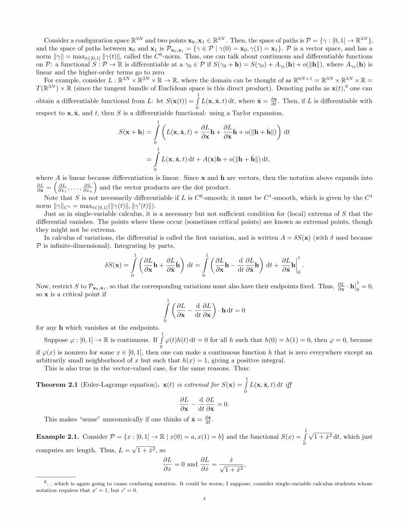
Theorem 2.1 (Euler-Lagrange equation). x(t) is extremal for S(x) =1∫0

L(x, x, t) dt iff

∂L

∂x− d

dt

∂L

∂x= 0.

This makes “sense” mneomnically if one thinks of x = dxdt .

Example 2.1. Consider P = x : [0, 1]→ R | x(0) = a, x(1) = b and the functional S(x) =1∫0

√1 + x2 dt, which just

computes arc length. Thus, L =√

1 + x2, so

∂L

∂x= 0 and

∂L

∂x=

x√1 + x2

,

6. . . which is again going to cause confusing notation. It could be worse, I suppose; consider single-variable calculus students whose

notation requires that x′ = 1, but c′ = 0.

4

and the Euler-Lagrange equation gives

d

dt

(x√

1 + x2

)= 0, which means that

x√1 + x2

= c

for some constant c. Thus, x2 = c1 for some other constant c1 after rearranging, and x(t) = c1t+ c2, with c1 and c2determined by the boundary values a and b. Thus, the shortest path between two points is a straight line.

None of the above required Cartesian coordinates, so everything works just as well in another coordinate system.For example, if a curve is given in polar coordinates r(t), ϕ(t), take unit vectors er and eϕ in these directions, then

x(t) = (r(t), ϕ(t)) and x(t) = rer + rϕeϕ. Since (er, eϕ) is orthnormal, then |x|2 =√r2 + r2ϕ2, so the arc length

functional can be done in polar form and Example 2.1 still works.Consider Xi ∈ R3 and x = (X1, . . . , XN ) ∈ R3N . According to Newton determinacy, miXi = Fi(x, x, t), where the

functions Fi are called forces. There is a class of mechanical systems in which Fi is dependent only on x, which givesa function U(X1, . . . , Xn) such that

miXi = Fi(x) = − ∂U

∂Xi(x). (1)

This system is called a potential system, and corresponds to a set of points moving in a potential field. Manyinteresting problems take this form; for example, the n-body problem has (up to units)

U =n∑

i,j=1

mimj

|Xi −Xj |.

However, this formalism is dependent on Euclidean coordinates, which is a problem. The Lagrangian formulation ismore general and therefore more useful.

Considering the potential system above, define the kinetic energy to be T =∑ m‖X2

i ‖2 and define U(X) to be the

potential energy. Then, let L : T (R3N )→ R (i.e. L is time-independent) be given by L(x, x) = T − U , the Lagrangefunction of the system.

There is a nuance here: Xi isn’t velocity or a derivative here, but should be thought of as coordinates in thetangent bundle, so that T computes some quadratic form on elements of the tangent bundle.

Theorem 2.2 (Least Action Principle of Hamilton). The Newton equations (1) are equivalent to the Euler-Lagrangeequations for L(x, x) = T − U .7

Proof.

S(x) =

1∫0

L(x, x) dt =

1∫0

(∑i

mi‖X2i ‖

2− U(X1, . . . , Xn)

)dt.

The Euler-Lagrange equation for this is ∂L∂Xi

= ddt

∂L∂Xi

, but ∂L∂Xi

= − dUdXi

and ∂L∂Xi

= miXi. Thus, this gives

− ∂U∂Xi

= miXi, which is (1).

Thus, if one takes two points in the configuration space, understanding how the system moves from one to theother is in a way that “minimizes” (actually extremizes, though this is usually minimizing) this action functional.This is powerful because it is independent of coordinates.

A (Lagrangian) mechanical system where L = T − U , T is a quadratic form depending on velocity and U dependson x1, . . . , xn is called a natural system. However, there are important systems for which L doesn’t take this form.

If a system has holonomic constraints (such that the configuration space is a submanifold Σ of R3N ), it can bethought of in two ways. The first is to think of it as a very powerful force pushing everything to Σ (so the configurationspace is thought of as R3N ). For example, if U is the potential function, one can make a new potential function

U(x) = U(x) + N dist2Σ (i.e. distance to the surface), where N is very large, so that the gradient points into the

surface and everything is pushed onto it. In the limit N →∞, the system is actually constrained to Σ, and cannotleave (e.g. in a rigid body, there is a force holding it together). Alternatively, one could just live on Σ, since there arealways local coordinates, and the Euler-Lagrange equation is coordinate-independent.

For the Hamiltonian formalism, which will be discussed later, there is even more invariance under change (andthus power), since it doesn’t require the coordinates in the tangent bundle to be induced from the coordinates on themanifold.

7Technically, S(x) =1∫0

L(x, x) dt, which is called the action function, is the equivalence.

5

Suppose M ⊂ R3N is a configuration space (some submanifold of R3N ). Then, TM is called the phase space, and

is a manifold of twice the dimension of that of M . Then, L : TM → R is the Lagrangian, and S(x) =1∫0

L(x(t)) dt is

the action functional. Any local system of coordinates on M are called generalized coordinates, typically denotedq1, . . . , qk. The dual coordinates q1, . . . , qk are called generalized velocity. Then, the ∂L

∂qi, typically written pi, are

called the generalized momenta and ∂L∂qi

are called generalized forces. Then, the Lagrangian equation looks like

pi = dLdqi

, which in specific cases implies pi = miqi, which is the definition of momentum in elementary physics classes,

so this formalism is fairly powerful. If L is independent of qi, then the generalized momenta are preserved (in whichcase the coordinates are called cyclic). In general, if L is independent of some quantity, a conservation law emerges.

3. Suddenly, Riemannian Geometry: 1/14/13

In Lagrangian mechamics, one starts with an n-dimensional manifold M called the configuration space of thesystem, and the system is said to have n degrees of freedom. For example, one particle moving in 3-dimensional spacehas 3 degrees of freedom and the configuration space is R3. For a system of N particles moving in 3-dimensionalspace, there are 3N degrees of freedom and the configuration space is R3N .

In a constrained system, the system is restricted to a submanifold, which is still called the configuration space. Forexample, the motion of a rigid body is a constrained system.

The tangent bundle TM is a 2n-dimensional manifold (and in particular is not a submanifold of whatever spaceM lies in). If (q1, . . . , qn) are local coordinates in an open neighborhood U ⊂ M , these coodrinates induce localcoordinates on TU ⊂ TM given by (q1, . . . , qm,

∂∂q1

, . . . , ∂∂qn

); the latter n coordinates represent velocity vectors.

Then, every tangent vector is written T =∑ni=1 qi

∂∂qi

. Here, the dot is only notational; here it doesn’t denote a

derivative with respect to time.Then, the Lagrangian formalism considers the Lagrangian function L : TM → R (in an autonomous, or time-

independent system) or sometimes L : TM × R→ R (non-autonomous, or time-dependent) L(q, q) or L(q, q, t) anda functional (i.e. a function on an infinite-dimensional space) on Pa,b = γ : [a, b] → M | γ(0) = a, γ(1) = b (the

space of paths on M from a to b, with a, b ∈M) S : Pa,b → R and given by S(γ) =1∫0

L(γ(t), γ′(t), t) dt.

This is usually written S(q) =1∫0

L(q, q, t) dt, since paths and coordinates are conventionally written with the same

letters. Here, q means both coordinates of the velocity vector and ddt , since a path p on M can be lifted into TM by

taking the velocity, which is why this notation is used.Formally, Pa,b ⊂ P(M) = γ : [0, 1] → M. There is also P(TM) = γ : [0, 1] → TM. Then, there is a lifting

map ` : P(M)→ P(TM) given by ` : γ(t)→ dγdt (i.e. γ′(t)).8 Thus, if Γ(T ) = `(γ(t)), then Γ is on TM , so one can

take1∫0

L(Γ(t)) dt.

We also have the least action principle of Hamilton (i.e. Theorem 2.2): if a system travels from a ∈M to b ∈Mover time, then the path it takes is an extremum for the action functional S (usually a minimum, but not always).

From the calculus of variations (and the previous lecture), the extrema of the action functional satisfy the Euler-Lagrange Equation (Theorem 2.1; called such in the calculus of variations, but just called the Lagrange equation inmechanics). This is a 2nd-order differential equation.

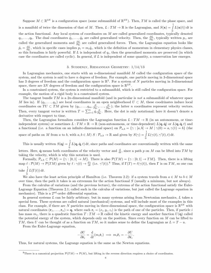
In general systems L can be fairly arbitrary. but in many systems arising from Newtonian mechanics, L takes aspecial form. These systems are called natural (mechanical) systems, and will include most of the examples in thisclass. For example, if there are N particles moving in three-dimensional space, the configuration space is R3N withnatural coordinates (r1, . . . , rn) = q, where each ri = (xi, yi, zi) is the path of one of the particles. Then, if particle ihas mass mi, there is a quadratic function T : TM → R called the kinetic energy and another function U(q) calledthe potential energy of the system, which depends only on the position. Since every function on M can be lifted toTM , then U can be thought of as a function on TM , so it makes sense to define the Lagrangian as L = T − u.

From the Euler-Lagrange equation,

−∂U∂ri

=d

dt(miri) =⇒ miri = −∂U

∂ri.

Thus, for natural systems, the Lagrange equation is the same as the Newton equations.

8There is a canonical projection P(TM)→ P(M), but lifting in the reverse direction requires a choice of coordinates.

6

This also holds true if M ( R3N (i.e. the system is constrained), which can be seen by modelling the constraint asa very strong force onto M . Then, T can be thought of as T on R3N restricted to M . In Riemannian geometry, thisis an example of an induced Riemannian metric.

Definition. Let M be a manifold and g : TM → R such that g is a positive definite quadratic form on (that is, whenrestricted to) any tangent space of TM . Then, g is a Riemannian metric.

A Riemannian metric induces a scalar product on each tangent space, so there is Euclidean geometry on everytangent space, which allows the calculation of (for example) arc length of curves on M . This leads to the subjectknown as Riemannian geometry.

The point of all this is that, while every manifold can be thought of as a submanifold of Euclidean space, thisapproach doesn’t require that and is thus more convenient; in a sense, it is non-exploratory.

For example, on the surface of Earth (approximately S2), one can introduce local coordinates at any point andmeasure things. Then, if u = (u1, . . . , un) and v = (v1, . . . , vn), then their scalar product will be some positive definitequadratic form

∑i,j aijuivj — but the coefficients aij do not need to be constant, and their variation describes the

geometry of the world.If q1, . . . , qn are coordinate functions, they induce the differential 1-forms dq1, . . . , dqn ( dqi is the ith coordinate

function for the linearization of a function at a given point). Then, each quadratic form can be written as∑aij dqi · dqj

(here, the dot is just scalar product).9 This is how the Riemannian metric is usually written in local coordinates.Thus, for a system constrained to M , the kinetic energy function T can be some Riemannian metric; in particular,

the coordinates for the quadratic form needn’t be constant. Then, U is some (usually positive definite) function, andL = T − U .

If the system has no external forces (i.e. U = 0), then

1∫0

L(q, q) dt =

1∫0

T (q, q) dt =1

2

1∫0

‖q(t)‖2 dt.

This latter quantity is called the energy or energy functional in Riemannian geometry.It is a lemma in Riemannian geometry that minimizers of energy are also minimizers of length (intuitively, one of

these minimizes ‖q‖ and the other minimizes ‖q‖2). These minimizing curves are called geodesics.Thus, Riemannian geometry is just a special case of Lagrangian mechanics for systems with holonomic constraints.

Also, note that masses were largely absent from the above discussion, since they were absorbed into the Riemannianmetric (and therefore they actually curve space, in some sense).

Now for some terminology: if some term exists in the Newton schema ddt (miri) = − ∂U

∂ri, then the generalized

version of that term exists for the Lagrange schema ddt∂L∂qi

= ∂L∂qi

. Thus,

• If q1, . . . , qn are local coordinates on M , they are called generalized coordinates (which doesn’t add any moremeaning).

• In the Newtonian schema, the − ∂U∂ri

are called forces, so the ∂L∂qi

= Fi are called generalized forces.

• The miri are called momenta, so the pi = ∂L∂qi

are called generalized momenta.

The Newton form of these equations is ddt (pi) = Fi.

If ∂L∂qi

= 0 (in which case the potential and kinetic energies are independent of the coordinate qi), the coordinate

qi is caled cyclic, and some quantity is preserved. In differential equations, this yields an integral of motion, whichallows one to reduce the order of the equation, making it easier to solve.

In the case where the Lagrangian is time-independent (autonomous), there is also a conservation law:

Theorem 3.1 (Conservation of Energy). In an autonomous system,10 define the energy to be

H = pq− L =∂L

∂qq =

∑ ∂L

∂qiqi.

Then, H is preserved; it is an integral of motion, so it is constant for every trajectory.

Proof. Trivial; differentiate.

d

dt

(L−

∑ ∂L

∂qi· qi)

=∂L

∂qq +

∂L

∂q

d(q)

dt− d

dt

(∂L

∂q

)q− ∂L

∂q

d(q)

dt.

Then, the first and third terms cancel out because of the Lagrange equation.

9Observe that this isn’t a bilinear form; that would be written something like∑aij dqi ⊗ dqj .

10This is a system where L doesn’t depend explicitly on t. There is an implicit dependence in the trajectories given by L.

7

H is also called the Hamiltonian, but not yet.

Theorem 3.2 (Euler equation for homogeneous systems). Suppose that L = T −U is a natural system: T =∑aij qiqj

and U is a function of q. Then,∂L

∂qq =

∑aij qiqj = 2T.

The coefficient appears because in the calculation of the sum of squares, the symmetry of the equation ensures everyterm appears twice.

Thus, L− q∂L∂q = −T − U .

Consider the motion of a particle in a field, so that L = m|r|22 − U(r), so that the equations of motion are

the standard Newton equations: mri = −∂U∂r . Suppose this field is symmetric to some axis; introduce cylindricalcoordinates (r, ϕ, z), where the axis of symmetry is in the z-direction.

Thus, r2 = x2 + y2 + z2 = r2 + r2ϕ2 + z2.11 Then, ϕ is cyclic (this is actually the source of the word), and themomentum pϕ− = ∂L

∂ϕ = r2ϕ is conserved. This is conservation of angular momentum about the z-axis; specifically,

the quantity r2ϕ = |r× r| is preserved, which is the area of the parallelogram spanned by r and r.

4. Examples of Natural Systems: 1/16/13

First consider a system with 1 degree of freedom, so that the configuration space is either a line or a circle. Then,L = x2/2 − U(x) and x = −U ′(x). This system is always integrable and therefore easy to solve: the energy is

E = x2/2 + U(x), which is conserved, so x = ±√

2(E − U(x)).To solve this equation, think of it as a Pfaffian equation (which gives a line field, since this system has one degree

of freedom), given by 0 = dx−√

2(E − U(x)) dt. Then, a solution can be obtained by rearranging to

dt =dx√

2(E − U(x))

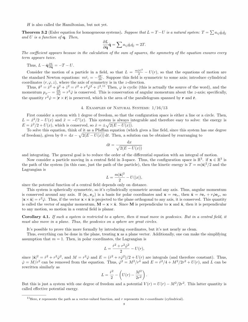
and integrating. The general goal is to reduce the order of the differential equation with an integral of motion.Now consider a particle moving in a central field in 3-space. Thus, the configuration space is R3. if x ∈ R3 is

the path of the system (in this case, just the path of the particle), then the kinetic energy is T = m|x|2/2 and theLagrangian is

L =m|x|2

2− U(|x|),

since the potential function of a central field depends only on distance.This system is spherically symmetric, so it’s cylindrically symmetric around any axis. Thus, angular momentum

is conserved around any axis. If (er, eϕ) is a basis for polar coordinates and x = rer, then x = rer + rϕeϕ, so|x× x| = r2ϕ. Thus, if the vector x× x is projected to the plane orthogonal to any axis, it is conserved. This quantityis called the vector of angular momentum, M = x× x. Since M is perpendicular to x and x, then it is perpendicularto any motion, so motion in a central field is planar.

Corollary 4.1. If such a system is restricted to a sphere, then it must move in geodesics. But in a central field, itmust also move in a plane. Thus, the geodesics on a sphere are great circles.

It’s possible to prove this more formally by introducing coordinates, but it’s not nearly as clean.Thus, everything can be done in the plane, treating x as a plane vector. Additionally, one can make the simplifying

assumption that m = 1. Then, in polar coordinates, the Lagrangian is

L =r2 + r2ϕ2

2− U(r),

since |x|2 = r2 + r2ϕ2, and M = r2ϕ and E = (r2 + rϕ2)/2 + U(r) are integrals (and therefore constant). Thus,ϕ = M/r2 can be removed from the equation. Thus, ϕ2 = M2/r4 and E = r2/4 + M2/2r2 + U(r), and L can berewritten similarly as

L =r2

2−(U(r)− M2

2r2

).

But this is just a system with one degree of freedom and a potential V (r) = U(r)−M2/2r2. This latter quantity iscalled effective potential energy.

11Here, r represents the path as a vector-valued function, and r represents its r-coordinate (cylindrical).

8

Solving this new system, one obtains r =√

2(E − V (r)), which can be rewritten in Pfaffian form as

dt =dr√

2(E − V (r)).

Thus, motion is given by ∫ t1

t0

dt =

∫ r1

r0

dr√2(E − V (r))

,

where r0 = r(t0) and r1 = r(t1). Additionally, it is possible to combine these equations and write

dϕ

dr=

M

r2√

2(E − V (r)). (2)

After integrating, ϕ can be found as a function of r.Since r2/2 + V (r) = E, then V (r) ≤ E, and at a minimum point (in which E is equal to a minimum of V (r)),

r is constant, which means that the particle moves in a circular orbit. If the constraint is between two values rmin

and rmax, then the particle orbits between the two circles given by rmin and rmax. The minimum value is called thepericenter, and the maximum is the apocenter.12

Computing the time needed to go from rmin to rmax is as easy as calculating

t =

∫ tmax

tmin

dt =

∫ rmax

rmin

dr√2(E − V (r))

,

and computing the angle between the pericenter and apocenter just requires plugging this into (2). Note that thisangle doesn’t change as the trajectory evolves. In particular, this angle ∆ϕ is either:

• commensurate with 2π, in which case the orbit is periodic, or• not, in case the orbit is everywhere dense between rmax and rmin.

Suppose the original potential energy is U(r) = rα. Then, there are exactly 2 values of α for which all solutions areperiodic: α = −1, which is the Kepler solution (all orbits are ellipses), and α = 2. This is pretty hard to show.

Consider the Kepler case, where U(r) = −k/r, so that V = −k/r −M2/2r2 and

ϕ =

∫ Mr2 dr√

2(E − V (r))=

∫ Mr2 dr√

2(E + k

r −M2

2r2

) .Let u = 1/r, so that

= −∫

M du√2E + 2ku−M2u2

= −∫

du√2EM2 + 2ku

M2 − u2.

Letting t = u− k/M2, this equals

= −∫

dt√2EM2 + k2

M4 − t2.

Let a = 2E/M2 + k2/M4.

= arccos

(t

a

)

= arccos

1r −

kM2√

2EM2 + k2

M4

,

up to some constant, which is just choosing the initial point of the pericenter.From this, one can express r through ϕ (or through cosϕ), obtaining r = p/(1 + e cosϕ), where p = M2/k and

e =√

1 + 2EM2/k2 is the eccentricity. This is the polar form of a conic section; for example, if 2c is the distancebetween the two foci of an ellipse and a is the semimajor axis, then e = c/a (so that e < 1 for an ellipse and e = 0

12In celestial mechanics, these are called the perigee and apogee, respectively.

9

for a circle, corresponding to negative energy; e = 1 for a parabola, corresponding to zero energy; and e > 1 for ahyperbola, corresponding to positive energy).

Consider an ellipse x2/a2 +y2/b2 = 1 and let c = a2− b2. Then, b = a√

1− e2 = a(1− e2/2 + . . . ), so the differencein the axes is in the second order of e, so an ellipse with small e is almost a circle.

Consider a satellite that is supposed to to orbit at a 300 km orbit, but was fired incorrectly, with a 1 deviationtowards Earth. Then, what is its perigee (or rather, what is the order of magnitude of the mistake)? It’s an uglycomputation, but since the mistake is very small and the velocity doesn’t change, then the orbit is still roughlycircular, displaced by 1. Thus, the displacement of this circle is equal to the distance between these two circles’centers, which is 6.7 · 107 · 2π/360 ≈ 110 km, which is actually quite a lot! (This is because r⊕ ≈ 6.4 · 107 m.)

For a completely different example, consider a system whose configuration space is the upper-half plane H = R2+ =

y > 0 with Riemannian metric (kinetic energy)

ds2 =dx2 + dy2

y2.

Here, ds measures the arc length, and the standard Euclidean metric is ds2 = dx2 + dy2. This looks similar, butthis system’s kinetic energy blows up as y → 0. This object is called the Lobachevsky hyperbolic plane, and is veryimortant in mathematics. The whole object can’t be realized in R3 with the usual Euclidean metric, but parts of itcan be.

If T = (x2 + y2)/y2 and there are no forces, computing paths is possible (albeit slightly ugly). L = T is independentof x, so ∂L

∂x = x/y2 is conserved. Thus, x = cy2. Additionally, since energy is conserved, then Ey2 = x2 + y2, so

y2 = Ey2 − c2y4.There are lots of isometries of this metric: the easiest example is translation along the x-axis, but another example

is homothety ((x, y) 7→ (cx, cy)). A more interesting isometry is called inversion, where (x, y) 7→ (x′, y′), such that|(x, y)||(x′, y′)| = 1. This is given by

(x, y) 7→(

x

x2 + y2,

y

x2 + y2

),

and plugging into the axioms verifies that it preserves distances and lengths. Finally, reflection across any verticalline is an isometry, since the metric is independent of x.

Thus, vertical lines are geodesics, and since these isometries can map any point to any point and any direction toany direction, then all geodesics are the image of a vertical line under isometries. In particular, under inversion, oneobtains semicircles around the x-axis. These vertical lines (which can be thought of as semicircles of infinite radius)and semicircles must be all possible isometries, since there is one for each point and direction.

Now consider H ⊂ C, given by Im z > 0. Then, these transformations are called M obius transformations, orconformal transformations, and are linear transformations of the form az+b

cz+d , with a, b, c, d ∈ R (up to coprime-ness).

This set of transformations forms a group called PSL2(R). The specific connections are: 1/z is an inversion composedwith a reflection, az is scaling, and z + b is translation. There is a nuance in that reflection is orientation-reversing,which doesn’t play too well with hyperbolic geometry, but the important point is that all of the isometries of Hpreserve the complex structure. Thus, all surfaces can have a hyperbolic metric, and the equivalence betweenhyperbolic geometry and complex analysis is one of the most fundamental things in mathematics. Specifically, atheorem in the 19th century showed this could only hold for three metrics: the Euclidean metric, the spherical metric,and this hyperbolic metric (also sometimes called the metric of constant curvature −1).

5. More on the Kepler Problem: 1/23/13

Consider once again a particle moving in a central field; the sign errors that may lie in last week’s lecture willbe fixed. Its motion is planar, so one can consider motion in polar coordinates in this plane. Then, its velocity isv2 = r2 + r2ϕ2 and the Lagrange function is L = 1

2 (r2 + rϕ2)− U(r). Since this is independent of ϕ (i.e. ϕ is cyclic),

then the angular momentum ∂L∂ϕ = r2ϕ = M is conserved. This allows the order of the equation to be reduced:

∂L

∂t=

d

dt

∂L

∂r

=⇒ r = −U ′(r) + rϕ2

= −U ′(r) +M2

r3

= −U ′(r) +d

dt

(−M2

2r2

).

10

Then, V = M2/2r2 +U(r), so r = −V ′(r), which is a Newton equation with one degree of freedom. Then, the rest ofthe previous argument follows (this time with the right signs).13

If X ⊂M is a submanifold and a critical point on the space of paths of M lies in the space of paths of X, then itis also a point there. But the converse isn’t necessarily true, so lifting from the plane to its tangent bundle doesn’tquite work; if one takes a variation of r and adds some variation of ϕ or ϕ, it isn’t necessarily a lift.14

Returning to the Kepler problem, in which U(r) = −k/r and V (r) = −k/r +M2/2r2, then r = −V ′(r) and thereis an energy integral E = V (r) + r2/2. Thus,

r =√

2(E − V (r)) =⇒ dt =dr√

2(E − V (r)).

Additionally, r2ϕ = M , so ϕ = M/r2. Thus,

dϕ =M

r2dt =⇒ ϕ =

∫M dr

r2√

2(E − V (r)).

In particular, the quadratic polynomial under the square root is a standard integral leading to an arcsin function.Solving it leads to

r =p

1 + e cosϕwhere p =

M2

kand e =

√1 +

2EM2

k2. (3)

These are equations for conic sections in polar coordinates.Consider an ellipse given by the equation x2/a2 + y2/b2 = 1. Here, c2 = a2 − b2 and e = c/a. if e = 0, it is a circle,

and if e > 1, one obtains a hyperbola. This can be plugged ito (3) to determine how to obtain specific orbits (e.g. aparabola requires E = 0).

Suppose the orbit is periodic (so that e < 1). Then, M = r2ϕ is twice the sectorial velocity (since the parallelogramhas twice the area of the triangle) and the sectorial velocity is M/2. In partcular, it’s constant (hello Kepler). If T isthe period, then T (M/2) is the area of the ellipse, so

TM

2= πab =⇒ T =

2πab

M.

Thus,

a =p

1− e2=

M2

2|E|M2=

k

2|E|since E < 0, and similarly

b =√a2 − c2 = a

√1− e2 =

k

2|E|

√2|E|M2

k2=

M√2|E|

=⇒ T =2πab

M=

2π

M

(k

2|E|

)(M√2|E|

)=

πk√2E3/2

.

Since 2E = k/a, then this becomes T = πa3/2/√

2k, which yields another of Kepler’s laws. This is a very rich subjectwith lots to explore.

Consider a Russian cosmonaut on a spacewalk who takes a camera out to take a picture and finds he has nowhereto hold his lens cap.15 He decides to throw his lens cap towards the Earth, but what happens? It turns out he will behit by it from above.

Exercise 5.1. Prove this.

The best way to approach this is to avoid all of the ugly theory, but consider the linearization of this system:r = −r/r3, up to units (so pick nice units which make this happen). Writing this in polar coordinates and writingvariations, the system starts with r0 = ϕ0 = 1 and is perturbed to obtain r = r0 + r1 and ϕ = ϕ0 = ϕ1 (with r1 r0).leaving only the linear term (not even constants) gives a mostly accurate description of the orbit and a system oflinear equations that can be solved.

Suppose a system has some symmetry, such as a 1-parametric group of transformations that preserves the Lagrangefunction. For example, if ϕ is a cyclic coordinate, then ∂

∂ϕ is a vector field that preserves the Lagrangian. Such a

vector field is called a symmetry. In this case, one can change coordinates so that the flow is in one of these directionsand obtain an integral. But this is somewhat inconvenient, so a simpler solution was found by Noether.16 First,though, a definition:

13The following assertions were wrong: that L = 1/2(r2 +M2/r2)− U ′(r) = r2/2− V (r), where V (r) = U(r)−M2/2r2.14To make life more confusing, this does work in the Hamiltonian case, since everything is set up differently.15This is supposedly a true story.16Noether was a great mathematician, but Theorem 5.1 is kind of trivial and not the entire reason.

11

Definition. A one-parametric group of transformations is a family of transformations gt : M →M (t ∈ R) such that

gt+t′

= gt gt′ (which implies a group structure).

This induces a vector field dgt(x)dt

∣∣∣gt(x)

= v, leading to a local flow. It also induces another group Gt : TM → TM ,

since the differential of gt operates on tangent spaces.

If gt : M → M is a symmetry of the Lagrangian system on M (i.e. L(Gt(x)) = L(x) or d(L(Gt(x)))dt = 0), then

dL(v) = 0 as well. Thus, it becomes necessary to compute dGt()dt as well (which is, oddly enough, tangent to the

tangent bundle). The final result is

0 =d(L(Gt(x)))

dt= dL(v) =

∂L

∂q· v =

∑ ∂L

∂qi· vi,

assuming some coordinates L(q, q, t). The flow is qi 7→ qi + t, which lifts upstairs (and the dot coordinates don’tchange at all).

Theorem 5.1 (Noether). Suppose the Lagrangian system L(q, q) admits a 1-parametric group of symmetries generatedby a vector field v. Then, I =

∑∂L∂qivi is an integral of motion.

Proof. First consider the special case v = ∂∂q1

, so that v is a symmetry iff q1 is cyclic. Then,∑

∂L∂qivi = ∂L

∂q1(i.e. the

generalized momentum corresponding to q1), so dIdt = 0.

The generalized case is the same, since one can always choose coordinates in which v = ∂∂q1

.

Consider a system of points with masses m1, . . . ,mk and coordinates r1, . . . , rk ∈ R3 moving in a potential field Uthat depends only on the distances ‖ri − rj‖. Then, the momentum

∑miri is an integral by Noether’s Theorem: the

Lagrangian is L =∑mi‖ri‖2/2− U , so L is independent by addition of any other vector (which is just translation).

Choose a basis e1, e2, e3 of R3; then, the vector field corresponding to ri 7→ ri+e1 is v = (1, 0, 0, 1, 0, 0, . . . , 1, 0, 0).Thus,

L =∑ m0(x2

i + y2i + z2

i )

2− U,

so the Noether integral is∑

∂L∂xi

=∑mixi. Thus,

∑mixi = 0 since the integral is constant.

In some sense, preservation of momentum is a corollary of Noether’s Theorem. Similarly, angular momentum,∑mi(ri × ri) is preserved in the case of rotational symmetry.

6. Rigid Bodies I: 1/28/13

The sutdy of motion of rigid bodies was a major focus of mathematics in the 19th Century. Rigid bodies can beanalyzed with the Lagrangian or Hamiltonian formalism; this lecture (as with the book) does the former.

The configuration space of a rigid body is M = R3 × SO(3), corresponding to a rotational frame frozen in thebody (whose orientation determines an orthogonal matrix in SO(3)) and a point that moves in R3.

Consider a rigid body in the absence of external forces, so that L = T , and approximate the rigid body as a set

of i points with locations qi and masses mi, so that T =∑ mi‖qi‖2

2 . If instead the density function is given by a

density distribution µ, then this becomes T = 1/2∫µ‖q‖2 dt. Since momentum is conserved, then

∑miqi (or the

corresponding integral) is constant. Equivalently, the center of mass, qC =∑miqi/

∑mi, moves with a constant

velocity. Sometimes, the center of mass is fixed at the origin, so the configuration space is just SO(3). Thus, a rigidbody in the absence of external forces moves as if fixed at a point.

Consider a rigid body fixed at a point (not necessarily the center of mass), so that the configuration space is SO(3).Pick some coordinates for R3, and denote this space k, and let K be some coordinate system fixed to the rigid body.Then, vectors in K will be denoted by uppercare letters, and those in k will be denoted by lowercase letters (the twospaces are the same, but with different coordinates, and a map relates them).

If q ∈ k, then there is a corresponding Q ∈ K such that q = B(t)Q for some orthogonal (but time-dependent)

operator B(t), the change-of-coordinates operator. Then, q = BQ + BQ and BQ = BB−1q. Then, BB−1 is ananti-self-adjoint (i.e. skew-symmetric) operator:

BB−1 = (BBT)T = BTB = −BTB = −B−1B,

since differentiation and taking a transpose commute.17 And a skew-symmetric operator has a remarkable form in

R3: if ω = (ω1, ω2, ω3) ∈ R3, then the operator qCq→ ω × q is skew-symmetric: 〈Cq, q〉 = 〈ω × q, q〉 = 〈q, q× ω〉 =

−〈q, Cq〉, since things can be moved cyclically.

17This is a more general fact about this Lie algebra. . .

12

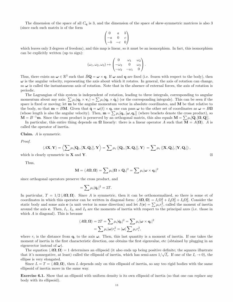
The dimension of the space of all Cq is 3, and the dimension of the space of skew-symmetric matrices is also 3(since each such matrix is of the form 0 a b

−a 0 c−b −c 0

which leaves only 3 degrees of freedom), and this map is linear, so it must be an isomorphism. In fact, this isomorphismcan be explicitly written (up to sign):

(ω1, ω2, ω3) 7→

0 ω1 ω2

−ω3 0 ω3

−ω2 −ω1 0

.

Thus, there exists an ω ∈ R3 such that BQ = ω× q. If ω and q are fixed (i.e. frozen with respect to the body), thenω is the angular velocity, representing the axis about which it rotates. In general, the axis of rotation can change,so ω is called the instantaneous axis of rotation. Note that in the absence of external forces, the axis of rotation isperiodic.

The Lagrangian of this system is independent of rotation, leading to three integrals, corresponding to angularmomentum about any axis:

∑µi(qi × vi) =

∑µi(qi × qi) (or the corresponding integrals). This can be seen if the

space is fixed or moving; let m be the angular momentum vector in absolute coordinates, and M be that relative tothe body, so that m = BM. Given that q = ω(t)× q, one can pass ω to the other set of coordinates as ω = BΩ(whose length is also the angular velocity). Then, m =

∑µi[qi, [ω,qi]] (where brackets denote the cross product), so

M = B−1m. Since the cross product is perserved by an orthogonal matrix, this also equals M =∑µi[Q, [Ω,Q]].

In particular, this entire thing depends on Ω linearly: there is a linear operator A such that M = A(Ω). A iscalled the operator of inertia.

Claim. A is symmetric.

Proof.

〈AX,Y〉 =⟨∑

µi[Qi, [X,Qi]],Y⟩

=∑

µi 〈[Qi, [X,Qi]],Y〉 =∑

µi 〈[X,Qi], [Y,Qi]〉 ,

which is clearly symmetric in X and Y.

Thus,

M = 〈AΩ,Ω〉 =∑

µi|Ω×Qi|2 =∑

µi|ω × qi|2

since orthogonal operators preserve the cross product, and

=∑

µi|qi|2 = 2T.

In particular, T = 1/2 〈AΩ,Ω〉. Since A is symmetric, then it can be orthonormalized, so there is some et ofcoordinates in which this operator can be written in diagonal form: 〈AΩ,Ω〉 = I1Ω2

1 + I2Ω22 + I3Ω2

3. Consider thestatic body and some axis e (a unit vector in some direction) and let I(e) =

∑µir

2i , called the monent of inertia

around the axis e. Then, I1, I2, and I3 are the moments of inertia with respect to the principal axes (i.e. those inwhich A is diagonal). This is because

〈AΩ,Ω〉 = 2T =∑

µi|qi|2 =∑

µi|ω × qi|2

=∑

µi|ω|r2i = |ω|

∑µir

2i ,

where ri is the distance from qi to the axis ω. Then, this last quantity is a moment of inertia. If one takes themoment of inertia in the first characteristic direction, one obtains the first eigenvalue, etc (obtained by plugging in aneigenvector instead of ω).

The equation 〈AΩ,Ω〉 = 1 determines an ellipsoid (it also ends up being positive definite; the squares illustratethat it’s nonnegative, at least) called the ellipsoid of inertia, which has semi-axes 1/

√Ii. If one of the Ii → 0), the

ellipse is very elongated.Since L = T = 〈AΩ,Ω〉, then L depends only on this ellipsoid of inertia, so any teo rigid bodies with the same

ellipsoid of inertia move in the same way.

Exercise 6.1. Show that an ellipsoid with uniform density is its own ellipsoid of inertia (so that one can replace anybody with its ellipsoid).

13

The 3-dimensional system (a 2nd-order equation) has 4 integrals: energy and the three angular momenta. But onthe phase space, this reduces to 2 1st-order equations (adding an extra coordinate), and such a differential equation isalways a vector field in R3. These integrals correspond to hypersurfaces (oh which all the trajectories must lie), so thetrajectories are on their intersection, which is a 2-dimensional manifold assuming the hyperplanes are all transverse.

In partiular, the vector field cannot have any zeros, so this manifold must be a torus (the only orientable manifoldfor which nice vector fields may be entirely nonzero). Motion on a torus must be quasiperiodic: ϕ1 = c1 and ϕ2 = c2(though the rotation may not be commensurate), which illustrates that this problem can be integrated explicitly.However, the general problem of a rigid body in a central field can’t be integrated, since two of the momentumintegrals are lost.

Since m = BM and m is constant, then M might be moving! Plugging it into the Euler equation yields M = [M,Ω](which can be viewed in terms of M or Ω, since M = AΩ), which can be solved to find Ω. This indicates how theaxis of rotation changes; then, the motion of the system is given by rotation arouhd the changing axis.

Here is the reason that M = [M,Ω]: m = 0, so

BΩ×BM = ω ×m = BM +BM = B(Ω×M) = B(Ω×M) +BM.

To solve this equation, move to the principal axes: M = (M1,M2,M3), Ω = (Ω1,Ω2,Ω3), and AΩ = (I1Ω1, I2Ω2, I3Ω3).

Thus, Ω = (M1/I1,M2/I2,M3/I3) and M1 = M2M3(1/I3 − 1/I2) + . . . , so M21 /I1 +M2

2 /I − 2 +M23 /I3 = 2E (the

energy expressed through m); this quantity is constant. The quantity ‖M‖ = ‖m‖ =√M2

1 +M22 +M2

3 is alsoconstant (thought M is not).

Thus, the trajectory is the intersection of this sphere and this ellipsoid, yielding three special cases:

(1) When the radius of the sphere is equal to the semiminor axis, the intersection is a point, so M is fixed, andthe motion is rotation about the fixed axis.

(2 and 3) The same for the other two axes. The smallest axis is Lyapunov stable, but the other is unstable, and adisplacement will push it away.

This is how motion looks to an observer on the rigid body.Applying B, to step outside, the solution moves smoothly around the ellipsoid, causing rotation about the axis,

which moves.

7. Rigid Bodies II: 1/30/13

Recall that a rigid body with one fixed point has configuration space SO(3). This is a system with 3 degrees offreedome, since SO(3) is a 3-dimensional manifold.

Each rotation is given by an axis and an angle; if this rotation is by an angle of less than π, then it can unambiguouslybe represented by a vector, where the magnitude represents the angle and the axis is given by the direction. But ifthe angle is π, there are two such possible points, causing an ambiguity. Topologically, this is fixed by “gluing” theopposite points together, and SO(3) is topologically equivalent to 3-dimensional real projective space. This is also thespace of lines through the origin in R4 (the space of one-dimensional subspaces), or the 3-sphere with opposite pointsidentified.

Studying the topological properties of a system tends to lead to qualitative physical properties. For example, SO(3)isn’t simply connected, so there exist loops which cannot be shrunk to a point. Of these non-contractible loops, takethe one with the smallest length; this loop is a geodesic. Thus, there is periodic motion!

Consider once again a system of coordinates k fixed to a body of motion, where K is the external system ofcoordinates, and use capital and lowercase letters as before: if x ∈ k, let X = B(t)x ∈ K. Motion is instantaneouslyrotation about some axis, but that axis may change with respect to time; denote this axis by ω or Ω, and denotethe angular monentum as m or M (so that ω = BΩ, and m = BM). m is constant, and M moves with the body:there exists a symmetric A such that M = AΩ, such that A depends only on the geometry of the body. Additionally,〈AΩ,Ω〉 = 2T , and if e is a unit vector, then the moment of inertia of the body about the e-axis is 〈Ae, e〉; if thesystem is made of discrete points with masses mi and distances from the e-axis ri, then 〈Ae, e〉 =

∑mir

2i (this will

be an integral in the continuous case).Since 〈Ae, e〉 is a positive-definite quadratic form, it is diagonalizable, so there are some axes in which 〈AΩ,Ω〉 =

I1Ω21 + I2Ω2

2 + I3Ω23 (so that the eigenvalues are the moments of inertia about the principal axis).

Theorem 7.1 (Steiner). Writing I(e) = 〈Ae, e〉 (through the line e), consider two lines e0, e1 separated by a distanceρ, such that e0 passes through the center of mass of the rigid body. Then, I(e1) = I(e0) + 2mρ2.

14

Proof. In the discrete case (the continuous case is similar),∑miri = 0, so∑

mi(ri + ρ)2 =∑

mir2i + 2ρ

∑miri +

∑piρ

2

= I(e0) +mρ2.

In particular, the moment of inertia is lowest through the axis containing the center of mass.The Euler equation can be written as dM

dt = [M,Ω]. Since M = AΩ, then the equation can be written in terms of

just one or the other; it is also [M, A−1M] (i.e. some quadratic equation in M). Writing this in principal coordinatesgives a quadratic system of 3 equations for dM

dt — which initially sounds complicated, but there are lots of integrals:

E = M21 /I1 +M2

2 /I2 +M23 /I3 is preserved, and ‖M‖2 = M2

1 +M22 +M2

3 is conserved as well. This means that themotion lies on the intersection of a sphere and ellipsoid, so an explicit but ugly formula can be written down, thoughit can’t be integrated with elementary functions. In fact, Jacobi invented elliptic functions for this purpose.

Thus, all trajectories are periodic, except when the sphere is tangent to the middle axis of the ellipse; this is calleda homoclinic orbit.

Definition. If O is a hyperbolic (i.e. unstable) point of a vector field and a trajectory starting from O returns to Oeventually, then O is called a homoclinic point.

“Now, we don’t want to be dizzy, so we view it from the outside, from the fixed coordinate system.”

Theorem 7.2 (Poinsot). Represent a rigid body by its ellipsoid of inertia with semi-axes 1/√I1, 1/

√I2, and 1/

√I3

(such that I1 ≤ I2 ≤ I3, so that the axes are in decreasing order). From stationary space, fix the center of the ellipsoid.Since the angular momentum m is fixed, then one can consider a plane tangent to the ellipsoid, orthogonal to m.

Then, the ellipsoid rolls around on the plane without slipping.18

This motion is actually somewhat complicated; if two of the axes are the same (in which case the ellipsoid is knownas an ellipsoid of rotation), the motion is circular, but not necessarily periodic. The ellipsoid also rotates around itsown axis, and if this isn’t commensurate with 2π, then it never repeats. In the general case, the curve isn’t evenclosed.

Proof of Theorem 7.2. Consider ω = BΩ, the axis of rotation of the ellipsoid. If one takes the normal vector to theellipsoid where ω intersects it, this vector must be parallel to m. Fixing the ellipsoid, the normal is the gradient ofthe function ∇〈AΩ,Ω〉 = 2AΩ = 2M (the derivative looks like this because the function is a quadratic form). Then,draw the plane paerpendicular to this normal at this point (so that it is perpendicular to m). Then, all that needs tobe checked is that the distance to this plane is constant.

A vector X on the elipsoid of inertia satisfies 〈AX,X〉 = 1, and 〈AΩ,Ω〉 = 2T , so scaling Ω requires scaline by√2T , so the distance from the center (i.e. the fixed point) to the plane is constant. Specifically, the distance is some

constant multiple of 〈Ω,m〉, or the length of the projection, and this is equal to 〈Ω,M〉 = 〈AΩ,Ω〉 = 2T , which isconstant.

The ellipse does not slip because its instantaneous velocity is always zero.

Exercise 7.1. Find a formula for the motion’s dependence on time in the case of an ellipsoid of rotation.

Now, suppose a rigid body moves in a constant field (i.e. a constant acceleration g, such as gravity). Consider atop: there is one fixed point, but it isn’t necessarily the center of mass. If ` is the distance between these two pointsand θ is the angle between the line and the vertical axis, then the Lagrangian is L = T − U = T −mg cos θ.

Here everything is harder; only one of the integrals of angular momentum is still here, and the phase spaceis 6-dimensional, so 2 integrals aren’t sufficient. In fact, an exact solution canot be computed (the system isnon-integrable).

However, suppose that this ellipsoid of inertia is also an ellipsoid of rotation, so that one obtains an extra integral(corresponding to rotation about that axis), which is already sufficient to integrate the system. The Euler angles aretwo cyclic variables that allow the integrals to be obtains let ex, ey, and ez be a fixed frame and let e1, e2, and e3

be coordinates in the moving system K. Let the angle between the vertical axes be θ, as before. Then, the planesperpendicular to ez and e3 intersect at the angle θ. Let eN be the unit normal on the line of nodes (referring to theintersection of the two planes — the name is due to Euler and has been religiously followed ever since). Let ϕ be theangle between ex and eN , and ψ be the angle between e1 and eN . These three angles θ, ϕ, ψ are the Euler angles.

One can rotate ex by ϕ, then around eN by θ, then e3 by ψ, in order to change one basis into the other. But thesystem is invariant under ϕ, so it’s cyclic. Additionally, ψ is cyclic (the axis of rotation), but θ isn’t cyclic, unless thesystem is totally fixed.

18This is an excellent physical model for ROFLing, as it happens.

15

Computing kinetic energy in these coordinates isn’t terribly simple. Note that the three rotations don’t commute,but infinitesimally, they do: the error is quadratic, so on the small scale it doesn’t make much of a difference. Then,for any point i in the body, its velocty is ω × ri. Here, ω = ωϕ + ωψ + ωθ = ϕez + ψe3 + θeN : the three anglesall change at some rate, so making this approximation has quadratic error. Since ϕ and ψ are fixed, the kineticenergy doesn’t depend on them, so suppose they are both zero, so that eN = e1 = ex, and the only rotation is in theezey-plane. This implies that

e3 = cos θez + sin θey

= ϕez + ψ(cos θez + sin θey) + θex

= ωxex + ωyey + ωzez =1

2〈AΩ,Ω〉 .

8. Rigid Bodies III: 2/4/13

The material on rigid bodies is hard to convey in lecture because of long computatiosn and such, so treat thislecture as a guide to reading the relevant chapter in the book.

Once again, denote the fixed coordinates as ex, ey, and ez, and the moving coordinates as e1, e2, and e3, where therigid body is symmetric about e3. Let θ be the angle between e3 and ez. Then, the exey-plane and the e1e2-planeintersect at a line; the coordinate in this line is eN . Then, ϕ is the angle between eN and ey, and ψ is that betweeneN and e1. These latter angles correspond to rotation of the body around an axis of symmetry. Additionally, assumea constant vertical field of gravity.

The Lagrangian is L = T − U = T −mg` cos θ, and T = 12 〈AΩ,Ω〉 = 1

2 (I1Ω21 + I2Ω2

2 + I3Ω23), but the goal is to

express it in the coordinates e1, e2, and e3.As shown last week, in the infinitesimal case rotation can be thought of as changing only one of the angles for the

purpose of calculating angular velocity. If only ψ changes, then the angular velocity is ψe3; similarly, if θ changes, itis θeN , and for ϕ it is ϕez.

In order to make everything nice, assume ϕ = ψ = 0. This is a dirty trick because we know the Lagrangiandoesn’t depend on them, so why even bother? This means that rotation will be in the e2e3-plane. This means thatex = eN = e1 and ez = e3 cos θ + e2 sin θ. Thus,

T = ψe3 + θe1 + ϕ(e3 cos θ + e2 sin θ)

= θe1 + ϕ sin θe2 + (ψ + ϕ cos θ)e3

=I12

(θ2 + ϕ2 sin2 θ) +I32

(ψ + ϕ cos θ)2,

since I1 = I2. Notice that this equation depends neither on ϕ nor upon ψ; what a surprise! Thus, Mz = ∂L∂ϕ and

M3 = ∂L∂ψ

are constant, yielding the following formulas:

Mz =∂L

∂ϕ= ϕ(I1 sin2 θ + I3 cos2 θ) + ψI3 cos θ

M3 =∂L

∂ψ= ϕI3 cos θ + ψI3.

With respect to ψ and ϕ, this is a system of linear equations, so they can be expressed in terms of Mz, M3, and cos θ.Solving this yields

ϕ =Mz −M3 cos θ

I1 sin2 θ,

which can be plugged into the energy conservation law:

E =I12θ2 +

(mg` cos θ +

(Mz −M3 cos θ)2

2I1 sin2 θ

)+M2

3

2I3.

The right-hand term is constant, and the whols system looks like one with a single degree of freedom; the left-handterm is referred to as the effective potential energy Ueff(θ).

This can be solved, but it’s very ugly and the resulting integral can’t be written in terms of elementary functions.One can thus make numeric approximations or qualitative observations.

It’s convenient to change variables: let u = cos θ, so that u2 = sin2 θθ2. Then, the equation becomes u2 = f(u) =(α− βu)(1− u2)− (a− bu)2 and ϕ = (a− bu)/(1− u2). where α, β, a, and b are constants in terms of Mz, M3, andso forth. Notice f is a degree-3 polynomial with a positive cubic coefficient. Then, f(±1) < 0 (since the square termis negative). If the maximum between −1 and 1 is positive, then there are two roots (and the third is meaningless,

16

since it would require |u| = | cos θ| > 1), and if not, there are none. If there are two roots u1 and u2, then motion hasto happen between them, and the motion changes periodically between two angles θ1 and θ2 (such that u1 = cos θ1

and u2 = cos θ2). Then, ϕ is the angular velocity around the vertical axis, so if ϕ has constant sign, then the toptraces a sinusoidal-like curve. But it may happen that things change sign, which yields a different picture, in whichthere may be loops. At a critical point, each curve has a cusp rather than a loop. Interestingly, this is an importantcase, and is physically observable, as in a spinning top starting at an angle.

The sign of ϕ depends entirely on a − bu, since 1 − u2 is always positive, so it is inportant whether u = a/b ispositive or negative.

Consider the special case of a slipping top: a small child tries to set up a top spinning perfectly vertically, so thatMz = M3 = I3ω3. Then,

Ueff =M1

3 (1− cos θ)2

2I1 sin2 θ+m2` cos θ

=

(M2

3

8I1− mg`

2

)θ2 +mg` = C +Aθ2

after some questionable computation, where C = mg` and A = M23 /8I1 −mg`/2. Then, consider small θ. θ = 0 is a

minimum of this function and is thus a stationary point. Everything depends on the sign of C and A: if A > 0, themotion is stable.19

If the top begins rotating at some other non-vertical angle θ0 and is rotating very fast, the main contributior tothe energy is 1

2I3ω2. The Lagrange function sacles by a constant factor (so the qualitative behavior is the same) if

the angular velocity is multiplied by C2 and the gravity is multiplied by C for some constant C; thus, a top spinningvery fast looks like a top spinning at a normal speed in very low gravity, so for now assume g = 0. Then, the effectivepotential energy is

Ueff =(Mz −M3 cos θ)2

2I2 sin θand the minimum energy is cos θ = Mz/M3 (which forces Mz ≤M3). Expanding at θ0, this implies that θ = θ0 + xfor some small variation x, and

Ueff =I23ω

23

2I1x2.

This implies that the equation of motion is I1θ/2 = −Ueff , or that θ = cθ for a constant c.This equation corresponds to a small oscillation with frequency

√c = ωnut called the frequency of nutation:

ωnut = I3ω − 3/I1. This is the frequency for how θ changes (though the rotation of the actual rigid body is morecomplicated than just a harmonic oscillator in the general case). Similarly, one can compute that ϕ is a harmonicoscillator with the same frequency.

Adding gravity back in shifts the minimum of the quadratic function Ueff very slightly, so the second derivativeeffectively doesn’t change, and the formula for nutation still approximately holds.

9. The Legendre Transform and Projective Duality: 2/6/13

Suppose y = f(x) is convex, or, more exactly, f ′ is a monotonically increasing map that is onto R. Then, the goalis to construct a functional on the dual space to R (i.e. the set of linear functions on R, each a function `(x) = px, so

the space is isomorphic to R). Then, define the Legendre transform of f to be a function f(p): if p ∈ R, then there is

exactly one x such that f ′(x) = p; then, the tangent line to f at x looks like y = px+ b. Then, f(p) = b.

More explicitly, f(p) = maxx∈R(px− f(x)) = px− f(x) where f ′(x) = p.

Example 9.1. If f(x) = x2/2, then f(p) = px − x2/2 where x − p, so it simplifies to p2 − p2/2 = p2/2, which ispretty nice.

If f(x) = mx2/2, then f(p) = px−mx2/2 where mx = p, so it becomes p2/2m, which is the expression for kineticenergy in terms of momentum.

Exercise 9.1. What is the Legendre transform of f(x) = xα/α?

Solution. It will end up as f(p) = xβ/β such that α−1 + β−1 = 1.

Here are some properties: f(p) ≥ px− f(x), so f(x) + f(p) ≥ px. This is called the Young Inequality. It also hassome non-obvious corollaries, such as xα/α+ pβ/β ≥ px, which is hard to prove explicitly.

If a function has a monotone derivative that doesn’t reach all values, the Legendre transform can still be computed:

if f(x) = ex, then f(p) = px− ex, with p = ex, so x = ln p. Thus, for positive p, f(p) = p ln p− p.

19Of course, if friction is accounted for, ω3 decreases, so M3 decreases, so the top falls.

17

Claim. The Legendre transformation of a convex f (such that f ′ is onto R) has the same properties of convexity.

Proof. Exercise.

Theorem 9.1. The Legendre transform is involutive:ˆf(x) = f(x) for any function f that meets the conditions.

Proof. This is sort of a tautology: f(p) = max(px − f(x)), soˆf(x) = max(xp − f(p)), since the double-dual is

naturally isomorphic to R. Then, px− f(p) is just the tangent line as a function, and at x it is just f(x).The goal is to find the tangent line with the greatest intersection with the vertical line through x, and it is a

property of convex functions that the maximum is f(x).

One can generalize into more dimensions: let V be an n-dimensional vector space, and let f : V → R be convex.More precisely, there is an orientation-preserving map given by the differential that is one-to-one.20 An example of aconvex function is any nondegenerate quadratic form.

Then, f(x) = maxx∈V (px − f(x)) = px − f(x) given p = df (so that pi = ∂f∂xi

for all i). Here, px can either

mean the dot product (so p ∈ V ) or as the function p(x) (so that p ∈ V ∗).This can be generalized yet further to the notion of projective duality. Projective space is an object of classical

mathematics. It is an unfortunate fact of Euclidean geometry that some lines don’t intersect (of course, the parallelones). People have been annoyed by this, so they defined a point at infinity that is the class of all parallel lines (sothat they “intersect” at infinity).

First consider the real projective space RP 2. There are many different models of this, but one is the space of linesin R3 through 0. If R3 has coordinates x, y, z, consider the plane xy = 1. Then, all lines in RP 2 intersect this planeat exactly one point, except for the one which is parallel (thus corresponding to adding one point). Similarly, one cantake the real line and compacitfy it by adding one point (as the space of lines through the origin in R2) to get theprojective line RP , which is topologically equivalent to a circle. This can be generalized to RPn, which can also bethought of as affine space An with RPn−1 attached.

Life in projective space is like a utopia. Everybody’s equal, and everyone intersects! But it’s even better: inEuclidean space, there are lower classes (points) and higher classes (lines), so that two points determine a line, butnot necessarily vice versa. However, in projective space, there is this kind of harmony: two points determine a line,and two lines determine a point.

Projective duality is the notion that there is a dual projective space where points go to lines and vice versa: send aline (as a hyperplane in Rn+1) to the point (i.e. a line in Rn+1) it is perpendicular to, and vice versa.21

Another nice fact is that in projective space, all quadratics are the same, only differing by how they intersect thepoint at infinity; all ellipses, parabolas, and hyperbolas are closed curves. An ellipse doesn’t intersect the point atinfinity; a parabola is tangent to it, and a hyperbola intersects it without being tangent.

The dual space has an affine part consisting of those lines which aren’t vertical (since they’re given by ϕ = px− b,so they can be seen as in R2). Take a graph of some function f on the projective plane, and take the space of all linestangent to it. Then, in the orthogonal construction, these become points which trace out a curve. If the functionis convex, this curve will lie in the affine part (since the tangent line is never vertical). This is just the Legendretransform!

Thus, the Legendre transform can be defined for nonconvex functions; if the function has an inflection point, itsLegendre transform has a cusp (that looks like the semicubical parabola x2/3), and vice versa. Similarly, if the tangentlines are ever parallel, the transform will self-intersect.

And projective duality is a special case of something much more general. . .Returning to mechanics: in Lagrangian mechanics, one has a configuration space M and a phace space, or tangent

bundle, TM = TqM | q ∈M, so that any local (generalized) coordinates q1, . . . , qn extend to a basis of TM given

by q1 = ∂∂q1

, . . . , qn = ∂∂qn

, so TM has the coordinates q, q, as a 2n-dimensional manifold.

Now, consider the cotangent bundle T ∗M . If q ∈ M , then T ∗qM is the dual space to TqM , the set of linearfunctionals on TqM , and T ∗M = T ∗qM | q ∈ M. Then, the coordinates q1, . . . , qn on M induce coordinates onT ∗M p1 = dq1, . . . , pn = dqn.

It happens that TM ∼= T ∗M , but the isomorphism is not canonical. However, if the manifold is Riemannian (i.e.every tangent space has a scalar product, and therefore a metric and a Euclidean structure), then thee is a canonicalchoice: V → V ∗ given by v 7→ v(x) = 〈v,x〉.

In the Lagrangian case, the Lagrangian is a function L : TM → R. In some nice systems called natural systems, Lis a positive-definite quadratic form on every tangent fiber and U depends only on q. Then, one can take the Legedretransform of this quadratic form. The Legendre transform also can be thought of as a map V → V ∗ that sends

20This has the odd consequence that convexity and concavity are only distinguished by orientation.21This also has the corollary that the spaces of lines and of hyperplanes are isomorphic, as with k-hyperplanes and (n− k)-hyperplanes.

18

x 7→ p = dxf (given an f on V ), or in coordinates, xi 7→ ∂f(xi)∂xi

. This is a diffeomorphism. Thus, the Lagrangian,

restricted to TM , induces a map TM 7→ T ∗M given by its Legendre transform. If L(q, q) is a quadratic in q, the

Legendre transform is H(q,p) = L(q,p), so H : T ∗M → R. This function H is called the Hamilton function, or theHamiltonian.

Working in coordinates, if L =∑miq

2i /2−U(q), then L =

∑piqi −

∑miq

2i /2 +U(q) such that pi = ∂L(q,q)

∂qi. (so

that qi plays the role of x). This is a system of n equations in n variables, so it can be solved, giving a Legendre

transform of L =∑pi/2m

2i − U(q). This is the kinetic energy again, but expressed in terms of the generalized

momenta ∂L∂qi

corresponding to the qi. Thus, the Hamiltonian is just the full energy of the system expressed in terms

of momentum rather than velocity.Recall that if q(t) is a trajectory in M , then it lifts to a trajectory on TM . But the map also induces a trajectory

q(t),p(t) that is almost completely equivalent, and considerably more powerful, so one can solve question in T ∗Mand then transmit the answers back to TM .

In the one-dimensional case, H(q, p) = max(pq − L(q, q)). The function being maximized is a function of threevariables G(q, q, p) (or G such that p = ∂L

∂q ). Let Γ be the hypersurface given by p = ∂L∂q , so there is a map

(q, p)S7→ (q, q) where p = ∂L

∂q . Thus, Γ is the graph of S and also of something else, because it’s one-to-one. Then,

q = Φ(q, p), so that H(q, p) = G(q, q = Φ(q, p), p).Then, the differential of H is a pullback: dH = S∗ dG (this is just restricting it to Γ and writing it in (q, p)-

coordinates). Most books get this wrong, and even Arnold doesn’t explain it (saying “I do not wish to breaktradition”). Let Gp denote the partial derivative with respect to p, and so on; then,

dG = Gp dp+Gq dq +Gq dq

= q dp+ p dq + Lq dq − Lq dq

= Φ dp+ pdΦ− Lq dq − Lq dq

This requires plugging in dΦ for q, which is what the pullback actually does. Then, dH falls out, giving a formula forHp and Hq: Hp = q, Hq = −Lq.

In general, nothing more can be said, but along the trajectory,

∂L

∂q=

d

dt

(∂L

∂q

)=⇒ dp

dt=∂L

∂q

=⇒ p =dp

dt= −Hq and q =

dq

dt= Hp.

This is a system of two first-order differential equations, called the Hamilton canonical equations, and it’s really niceand symmetric. A system of first-order differential equations is a vector field, so a trajectory is just an integral of thisfield. Diffeomorphisms of this vector field (called canonical transformations in mechanics or symplectomorphisms inmathematics) preserve the form of these equations, so there are a lot more options for cyclic coordinates. And if thereare n cyclic coordinates, the system is explicitly integrable, so one calls in symplectic geometry to answer these sortsof questions.

10. The Least Action Principle in Hamiltonian Mechanics: 2/11/13

Recall some stuff from last week: if M is the configuration space of some system, then TM is the phase spaceconsidered in Lagrangian mechanics. Every coordinate system q on M induces coordinates q on TM . The dymanicsof this system are given by the Lagrangian L : TM → R. In some systems, called natural systems, L = T − U , whereT is a fiberwise positive-definite quadratic form and U doesn’t depend on q.

The Hamiltonian formalism considers the cotangent bundle T ∗M (the space of linear functions). A section of thetangent bundle is a vector field, but a section of the cotangent bundle is a linear function associating a linear functionto each point, so it is a differential 1-form. The coordinates q1, . . . , qn on M induce coordinates p1 = dq1, . . . , pn = dqnon T ∗M , often denoted (q,p).

The Legendre transform can be used to move between the tangent and cotangent bundles. On some vector spaceV , one obtains orientation-preserving diffeomorphisms V → V ∗ such that x 7→ dxf . Then, f(x) is transformed into

some other function f(p) = px− f(x) at the maximum, so p = f ′(x). This should be understood as a system ofequations, so x can be expressed in terms of p.

On each tangent space, the Lagrangian is a convex function (in the case of natural systems and some others), sothe Legendre transform can be applied parametrically, with q ∈M as the parameter. Then,

L(p,q) = pq− L(q, q)|p= ∂L∂q. (4)

19

This Legendre transform is usually denoted H(p,q), and is called the Hamiltonian function on the system.22 TheLegendre transform not only acts on functions, but can also act as a more general map on spaces.

Be careful of a nuance: usually, one can take pullbacks to compute the results of diffeomorphisms. However,suppose that X and Y are two sets and h : X → Y is one-to-one. Then, if f : Y → R, then h∗f = f(h(x)) is afunction from X → R. if g : X → R, then g h−1 is a function on Y . This can always be done with this kind of map:it induces isomorphisms of functions. In the Hamiltonian case, this is exactly what is being done in (4), but puttingthe pq in front means it’s not quite that simple.

Thus, systems can be mapped to paths in the cotangent bundle. These paths satisfy the following equations in

local coordinates: p = dpdt = −Hq(p,q) and q = dq

dt = Hp(p,q) (the Legendre transform of ddt

(∂L∂q

)= ∂L

∂q ).

Physically, this can be thought of as passing from velocities to momenta; H is the full energy of the systemexpressed in terms of the momentum; U is constant in the transform.

Write u = (p,q), so that u = (−Hq, Hp). This is a first-order system of differential equations, and it is therefore

also a vector field XH = −Hq∂∂p +Hp

∂∂q (where the vector fields ∂

∂pi, ∂∂qi

are the unit vector fields,23 or the vectors

with velocity 1 in the directions pi and qi), and the trajectory is u = XH(u).Consider the special case when M = Rn. Then, T ∗Rn = R2n with coordinates (p1, . . . , pn, q1, . . . , qn), which we

will want to think of as R2n = Cn with coordinates (p1 + iq1, . . . , pn + iqn). If H(p,q) is the Hamiltonian, then its

gradient is ∇H =(∂H∂p ,

∂H∂q

). Thus, XH = i∇H.

Geometrically, the level sets of ∇H are the level sets of the full energy. Then, the gradient is normal to these levelsets H(p,q) = c, so multiplying by i makes things tangent to these level sets. Then, conservation of energy becomesobvious: since XH is always tangent to the level sets, then all trajectories must lie on these level sets.

Example 10.1. Consider H = 12 (‖p‖2 + ‖q‖2). If H = E (i.e. some constant), then the level set is the sphere

of radius√E. Thus, ∇H = p ∂

∂p + q ∂∂q . In a real vector space, every point belongs to a line, and in a complex

vector space, every point intersects a complex line (a plane), so each line has a plane, which determines a circle thatintersects with the sphere. The sphere is the union of such circles, which is referred to as a cofibration. If this is

generalized to an ellipsoid, there are n different closed orbits, and everything else is not closed: if H =∑ni=1

p2i +q2i2a2i

,

the closed sets happen only when intersecting with one of the complex axes.

Recall that in Lagrangian mechanics, the least action principle states that if γ is a path between q1,q2 ∈M . Then,

if γ is lifted to TM , then the principle claims that the paths are those which extremize S(γ) =∫ 1

0L(γ, γ, t) dt.

In Hamiltonian mechanics, the least action principle is considerably more powerful. Take any path γ(t) = (p(t),q(t)),where γ(0) = (p0,q0) and γ(1) = (p1,q1). Other than the boundary conditions, there are no constraints on p and q.

Theorem 10.1. On this class of paths,24 the system travels on a path that minimizes S(γ) =∫γ(p dq−H) dt.

In coordinates, there exists a differential form p dq =∑ni=1 pi dqi. There is a coordinate-invariant definition of this

form, however; since a differential 1-form is a linear map on each cotangent fiber, vectors can be projected from thecotangent bundle to M via π : T ∗M →M . Then, dπ : T (T ∗M)→ TM . If v ∈ Tq,p(T ∗M), then dπ(v) = Tq(M),but since p ∈ TqM , then p is a linear function, so p( dπ(v)) is a number, and p( dπ(v)) = p dq(v), which is thesame thing that was done in coordinates. Thus, the form p dq is universal, independent of coordinates. However, incoordinates induced from M , it always has the form

∑pi dqi.

Evaluating the action functional, if γ(t) = (p(t),q(t)), then

S(γ) =

∫γ

p dq−H(p,q) =

∫γ

∑pi dqi −H(p,q) =

∫ 1

0

(∑pi(t)qi(t)−H(p(t),q(t))

)dt.

For this function, the Euler-Lagrange equation is easy to write down, but since there is a different boundary condition,some proof is necessary. Consider a variation

S(γ + δγ) =

∫ 1

0

(p0 + δp)(q0 + δq)−H(p0 + δp,q0 + δq) dt

=

∫ 1

0

(p0q0 −H(p,q)) dt+

∫ 1

0

(δp0q0 + q0δq0 −

∂H

∂pδp− ∂H

∂qδq

)dt

22In terms of the meanings of the coordinates, H(q,p) would be a more natural ordering, but tradition and the alphabet have ensuredthat H(p,q) is most commonly seen.

23This at first peculiar notation is used because when the vector field is thought of as an operator of differentiation, these coincide with

partial differentiation in the appropriate direction.24This class of paths is much larger, and is in fact 2n-dimensional. This is the source of power of Hamiltonian mechanics.

20

plus some higher-order terms. At a critical point, this variation should be zero, so

=

∫ 1

0

(δp0q0 + δq0p0 −

∂H

∂pδp− ∂H

∂qδq

)dt

=⇒∫ 1

0

δqp0 dt = δqp0|10 −∫ 1

0

δqp0 dt

after integrating by parts. Then, if q is fixed, then the first term goes to zero (hooray for boundary conditions!), sowhen all of the terms are collected, ∫ 1

0

δp

(q0 −

∂H

∂p

)+ δq

(p0 −

∂H

∂q

)dt = 0

for all δp and δq. This implies that q = −∂H∂p and p = ∂H∂q , which was a variational proof of the Hamilton equations.

There are many other boundary conditions that work; for example, if the space of paths is such that momenta (orequivalently, velocities) are zero at the endpoints, or at only one endpoint, things still work; this has many usefulapplications.

The form p dq is important for Hamiltonian mechanics, but there is a more important form called the symplecticform, d(p dq) =

∑pi ∧ qi. This is related to the quite important interpolation between real coordinates in R2n and

complex ones in Cn.A bilinear function is a function f(x,y) that is linear in each argument. A function can be complex bilinear (i.e.

f(λx,y) = f(x, λy) = λf(x,y) for any λ ∈ C). If f is complex-valued, then it has real and imaginary parts, and it ispossible to obtain from this a complex form whose real part is invariant under multiplication by i. However, if thefunction is bilinear, it’s not possible to obtain anything interesting, so consider instead a Hermitian form, for whichf(λx,y) = f(x, λy), or f(x,y) = f(y,x), where f is linear in the first argument.

There are some standard Hermitian forms, such as f(x,y) =∑xiyi. For example, if x, y ∈ C and x = p + iq,

y = u+ iv, then xy = (pu+ qv) + i(pv − qu) = xy + i det(x, y).25 It turns out that the real part of any Hermitianform is symmetric, and the imaginary part is always skew-symmetric.

If R2 has some linear functions p and q, then there is a bilinear form called the exterior product: p ∧ q(x,y) =det(p(x), q(y)). In higher dimensions one obtains p1 ∧ q1 + · · ·+ pn ∧ qn. This is called the symplectic form.

Claim. Suppose V is a real vector space and F is a skew-symmetric bilinear function on V . Then,

(1) If F is nondegenerate, then dimV is even. (This is clear because det(AT) = det(A) = det(−A) =(−1)n det(A).)

(2) Given any nondegenerate, skew-symmetric, bilinear form, there exists a coordinate system (p1, , q1, . . . , pn, qn)such that F =

∑nj=1 pj ∧ qj .

Thus, up to change of coordinates, this form is unique, which is an amazing property of skew-symmetric forms(which is completely untrue for, e.g., symmetric quadratic forms).

11. Some Linear Algebra: 2/20/13

Let V be a vector space and F be a bilinear function on V . Every bilinear function is determined, in a basisv1, . . . ,vn, by F (X,Y) = XTAY, where aij = F (vi,vj). If F is skew-symmetric, so that F (X,Y) = −F (Y,X),then A is as well, so that AT = −A.

Exercise 11.1. Show that if A is the matrix of a skew-symmetric operator, then its rank must be even.

This implies in particular that if A has maximal rank, its determinant is nonzero, so dimV is even. If this is thecase, then F is called nondegenerate. Such a form can only exist in an even-dimensional vector space.26

If F is a bilinear form and X is a vector, one can create a linear function by contraction: X F is given byX F (Y) = F (X,Y). Thus, F is nondegenerate if contraction with a nonzero vector gives a nonzero function.

25In the higher-dimensional case, this generalizes to∑

i det(xi, yi), viewing each complex number as a 2-dimensional vector.26An equivalent and more natural definition for nondegeneracy is that for all nonzero X ∈ V , there exists a Y such that F (X,Y) 6= 0.

21

Theorem 11.1. Let F be a nondegenerate, skew-symmetric bilinear function on V . Then, there exists a basise1, f1, . . . , en, fn of V such that the matrix of F has the form

0 1−1 0

. . .0 00 0

.... . .

...0 00 0

. . .0 1−1 0

This is equivalent to the following:

• F (ei, fi) = 1 for all i, and• F (ei, fj) = F (ei, ej) = F (fi, fj) if i 6= j.

This means that if coordinates in this basis are denoted x1, y1, . . . , xn, yn, then F =∑ni=1 xi ∧ yi.

Proof. Proceed by induction on n (where dim(V ) = 2n).If n = 1, then let e be any vector. Then, there exists an f such that F (e, f) 6= 0. Thus, f can be normalized such

that F (e, f) = 1.Suppose this holds true up to n − 1. Then, let e1 be any vector, and find a corresponding f1, which will make

up the first block. Let L = span(e1, f1), and consider L⊥F = Z ∈ V | F (Z,X) = 0 for all X ∈ L.27 Then,dim(L) + dim(L⊥F ) = dim(V ) by Exercise 11.2 below, so dim(L⊥F ) = 2n− 2, and L⊥F t L (i.e. they intersect eachother transversely, since they intersect only at the origin). By induction, there is a basis e2, f2, . . . , en, fn in which Ahas the right form, so adding on e1 and f1 leads to the desired matrix.

Exercise 11.2. Show that, in the above proof, if F is nondegenerate, then dim(L) + dim(L⊥F ) = dim(V ). This canbe done by reducing it to a system of equations.

This is a remarkable result — there is a whole zoo of symmetric forms, but there is only the one skew-symmetricform. This suggests that it is important.

Choose the standard basis e1, f1, . . . , en, fn of R2n and let ω =∑xk ∧ yk. R2n can also be viewed as a complex

vector space Cn, where multiplication by i is defined as iej = fj and ifj = −ej . This can be thought of as a linearoperaotr whose square is − Id. Then, one jas complex coordinates zk = xk + iyk.

Here one can consider Hermitian forms. There is a unique positive-definite Hermitian form up to change ofcoordinates: if z = (z1, . . . , zn) and w = (w1, . . . , wn), then H(z,w) =

∑ziwi.

Claim. The real part of H is 〈z,w〉 =∑xkuk + ykvk (if zk = xk + iyk and wk = uk + ivk), and the imaginary part

is −ω(z,w).

Proof. It’s sufficient to check for n = 1, which is essentially the same thing: zw = (x+iy)(u−iv) = (xu+yv)−i(xv−yu).

Then, the real part is 〈w, z〉 and the imaginary part is

∣∣∣∣x uy v

∣∣∣∣ = ω(z, w).

H(iz, iw) = H(z,w) by the Hermitian property, so both the imaginary and real parts are invariant undermultiplication by i. But if g denotes the standard scalar product, then H(iz,w) = iH(z,w) = ig(z,w) + ω(z,w) =g(iz,w)− ω(iz,w). Thus, equating real and imaginary parts, g(iz,w) = ω(z,w) and ω(iz,w) = −g(z,w) (which isthe same thing, really).

Definition. A subspace L ⊂ V (where V is a symplectic space, or a space with a symplectic form ω) is calledisotropic if ω|L = 0 (i.e. ω(x,y) = 0 for any x,y ∈ L).

Example 11.1. The trivial subspace is of course isotropic (and if ω were replaced with a symmetric form, this wouldbe the only one). Another more interesting example is spane1, . . . , ek or spanf1, . . . , fk.

Exercise 11.3. Show that if L is an isotropic subspace, then dimL ≤ n. (As a hint, take the ω-orthogonal complementand then use the nondegeneracy of the form.)

Isotropic spaces of dimension n are called Lagrangian subspaces, and really play a central role in symplecticgeometry and Hamiltonian systems. A quick check of the definition shows that Lagrangian spaces are precisely thosefor which L⊥ω = L. Since ω(x,y) = 〈ix,y〉, then L⊥ω = iL⊥, so if L is multiplied by i, then it becomes its ownorthogonal complement!

27The usual orthogonal complement is the one for which F is the scalar product.

22

Figure 2. The Tropic of Cancer and the Tropic of Capricorn as isotropic subspaces of S2, the Earth.

Suppose L is Lagrangian and graphical with respect to the coordinates x = (x1, . . . , xn) and y = (y1, . . . , yn).Then, L is the graph of a symmetric linear function: L = y = Ax, and the converse is also true: if z = (x, Ax), z =(x, Ax) ∈ L, then ω(z, z) = 〈iz, z〉 = −〈Ax, x〉+〈x, Ax〉 = 0, so A is self-adjoint and can therefore be made symmetric.

If V is a symplectic space, the set of ω-preserving transformations (F : V → V such that F ∗ω = ω, orω(F (x,y)) = ω(x,y), so that F is also called symplectic) form a group, called the symplectic group Sp(V, ω). IfV = Cn, this is sometimes also written Sp(2n). The group of matrices that preserve the Hermitian operator iscalled the unitary group U(n), and those that preserve the Euclidean structure are called orthogonal, O(2n), so thatU(n) = O(2n) ∩ Sp(2n) by the above. Thus, acting on Rn by any unitary operator gives an isotropic subspace.

Now let’s throw in some differential geometry; instead of thinking of ω as a bilinear form, think of it as adifferential form (i.e. a bilinear form originating at any point). Then, ω =

∑ni=1 dxi ∧ dyi: this is the same form, but

parallel-transported, so that it can be applied to vectors originating anywhere.

Definition. If Ω1,Ω2 ⊂ R2n (as a symplectic space) and f : Ω1 → Ω2 is a diffeomorphism28 but not necessarily linear,then f is called a symplectic diffeomorphism or symplectomorphism if it preserves the symplectic form: f∗ω = ω, orω( daf(x), daf(y)) = ω(x,y) for all a ∈ Ω1 and x,y ∈ Va.

Theorem 11.2 (Darboux). Let ω be a nondegenerate (i.e. nonzero everywhere), closed (i.e. dω = 0) differential2-form on some domain U . Then, for any a ∈ U , there exists a neighborhood Ω ⊃ U of a and a symplectomorphismF : (Ω, ω)→ (Ω ⊂ R2n, ωst =

∑dxi ∧ dyi).

This theorem, which will be proven later, implies that F ∗ωst = ω, so F defines coordinates. Thus, this theoremimplies that in some neighborhood of a, there are some coordinates in which ω has the canonical form. This is thecomplete analogue of the linear case: the symplectic form is still very unique locally.

This can be globalized:29 let M be a 2n-dimensional manifold and ω be a closed, nondegenerate differential 2-form.Then, (M,ω) is called a symplectic manifold, and Darboux’s Theorem says there are local coordinates, called Darbouxcoordinates, in which M looks like R2n with the standard symplectic form.

If n = 1, every differential 2-form is of the form f(x, y) dx ∧ dy, and is therefore trivially closed, and Darboux’sTheorem says this can be reformulated as dx ∧ dy. This leads to the notion of area. Similarly, a symplectic structurein four-dimensional space allows integrating the symplectic form over any two-dimensional surface.

One important example of a symplectic manifold is M = T ∗N , where N is some n-dimensional manifold. Ifq1, . . . , qn are local coordinates on N and p1, . . . , pn are dual coordinates on the cotangent fibers, then let λ =

∑pi dqi,

which is a 1-form. Then, dλ =∑

dpi ∧ dqi is the symplectic form, so on the phase space of any mechanical systemthere is a canonical symplectic structure (i.e. λ can be defined without any coordinates).

Recall that the Hamilton function is H : T ∗M → R, with p = −∂H∂q , q = ∂H∂p , and ω = dp ∧ dq (in coordinates).

If XH is the vector field associated with these coordinates, then XH ω = dH. As a sanity check, if XH = a ∂∂p + b ∂∂q ,

then a dq− b dp = XH dp ∧ dq = −∂H∂p dp + ∂H∂q dq, so a = −Hq and b = Hp, which is exactly what was given for

XH .

28That is, it is at least C1-smooth, but one can assume C∞ for now; it is invertible; and f−1 is also at least C1-smooth.29If you wish to globalize literally as well as metaphorically, let M = S2n.

23

12. The Lie Derivative and the Poisson Bracket: 2/22/13

Let N be the configuration space of some mechanical system, and T ∗N be the phase space. On T ∗N , there isa canonical 1-form λ = p dq (with the notation chosen because in any set of coordinates q1, . . . , qn on N and theinduced coordinates p1, . . . , pn on T ∗N , λ =

∑pi dqi). Then, mechanics is defined by a function H : T ∗N → R. This

defines a vector field

XH =

n∑i=1

−∂H∂qi

∂

∂pi+∂H

∂pi

∂

∂qi, (5)

and trajectories correspond to integral curves of the system (so that pi = −∂H∂qi and qi = ∂H∂pi

). In order to get an

equation in this form, it’s not just unnecssary to choose specific p,q-coordinates, but in fact one can use much moregeneral coordinates than the induced ones, since it’s only necessary to know ω = dλ =

∑dpi ∧ dqi.

30

Thus, if R2n has coordinates q1, . . . , qn, p1, . . . , pn, then there is an invariant way to obtain the Hamilton canonicalequations given H(p,q). Given a nondegenerate bilinear form Φ, one has an isomorphism V ∼= V ∗ given by v 7→ v Φ;since this is a nondegenerate linear function between spaces of the same dimension, it is an isomorphism. Thus,v 7→ v ω induces an isomorphism Vect(U)→ Ω1(U) (the spaces of vector fields and differential forms, respectively).Denote by I the inverse of this map, which allows one to obtain vector fields from differential forms.

If n = 1, v = a ∂∂p + b ∂∂q , so v dp ∧ dq = a dq − b dp (the minus sign occurs because the order is reversed). Thus,

given an H, take dH = Hp dp+Hq dq, so the corresponding vector field is v = Hq∂∂p −Hp

∂∂q . This is identical to

the equations above, up to sign, so XH = −I( dH). Note that in higher dimensions this argument is essentially thesame, with the addition of indices. Be warned, however: there is no way to choose signs in a reasonable, natural way.Different books tend to have different sign conventions; for example, Arnold defines contraction by placing the vectorin the second argument, which means that XH = I( dH).

Thus, in order to define Hamiltonian mechanics, the only necessary ingredients are the phase space M with someclosed nondegenerate differential 2-form ω. M doesn’t need to be the cotangent bundle of anything, but can be anysymplectic manifold, and indeed such examples appear in applications. For example, if one wants to find integrals ofa system, a method called reduction sends a 2n-dimensional manifold to a (2n− 2)-dimensional one (which might notbe a cotangent bundle).

Dynamics are determined by some function H : M → R, the full energy of the system.31 Then, mechanics isdetermined by the vector field XH = −I( dH), or XH ω = − dH. Then, if u(t) is a trajectory, then u(t) = XH(u(t)).

A mechanical system has degrees of freedom, usually defined as the dimension of the configuration space; withoutthe configuration space, they can be defined as half the dimension of the phase space. If a system has 1 degree offreedom, then the phase space is a surface, so the symplectic form is an area form f(p, q) dp ∧ dq. Suppose A is aclosed surfact or a compact region with boundary and ω1, ω2 are two area forms with the same total area (so that∫Aω1 =

∫Aω2). Then, there exists a diffeomorphism f : A→ A such that f∗ω1 = ω2. Thus, the area form is unique,

though this is very untrue of the symplectic form in higher dimensions.Consider a smooth vector field X on a manifold M (we’ll be interested particularly in the Hamiltonian vector

field). If the manifold is compact or has the appropriate boundary conditions, then the vector field integrates to a

phase flow Xt : M →M , a 1-parametric group of diffeomorphisms, such that dXt(x)dt = X(Xt(x)). Locally, this flow is

always defined, and globally it depends on the conditions mentioned above (since otherwise, it could go to infinity).Then, finding the phase flow is equivalent to solving the differential equation u = X(u) for arbitrary initial data.M can be thought of as a compelx manifold, in which case XH = i∇H. Thus, XH is tangent to the level sets of

H, so all dynamics lie inside the level sets. This implies that energy is conserved.Returning to R2 with dp ∧ dq, consider H(p, q) = (p2 + q2)/2, so that p = −q and q = p, so that the phase

flow is just rotations. If H(p, q) = p2 + 2q2, one has ellipses (with the major axis in the q-direction). Consider thetransformation (p, q) 7→ (λp, q/λ) for some λ > 0; this is a canonical transformation, because dp ∧ dq is unchanged.

Thus, the second system can be changed into λ2p2 + 2q2/λ2 (setting p = λp and q = q/λ). Then, if λ = 4√

2, this isjust the first system, H(p, q) = p2 + q2, up to a scaling factor. Thus, the system can be easily solved and passed backto the original coordinates. This is an example of the power of the Hamiltonian formalism; the second system can infact be explicitly solved, but in general this might not be the case.

Suppose X is a vector field. If f is any function, one can take directional derivatives of the function as

daf(x) = limt→0

f(a + tx)− f(a)

t.

30In order to clear up something potentially confusing,∑pi ∧ qi is a bilinear form on Rn, which accepts vectors that originate at the

origin, but∑

dpi ∧ dqi is the same thing, except that since it’s a differential form, the vectors can originate anywhere.31Systems are assumed to be conservative; otherwise H would depend on time.

24

This moves points linearly, but one also can take the flow Xt, which provides the alternate definition of ∂∂tf(Xt(u))|t=0.

This is the formal definition of the Lie derivative, and is a viewpoint used in some other situations (such as quantummechanics). Though these formulas are equivalent, the latter one is a much better way to go about things, because itcan differentiate any more objects.32 The Lie derivative can also be given by d

dt (Xt)∗f .

Similarly, if ω is a differential form, the Lie derivative is LXω = ∂∂t ((X

t)∗ω)|t=0, and the Lie derivative for a vectorfield can be defined in an analogous way. Differential forms in particular obey something called the Cartan formula,as seen in Math 53H: if X is a vector field and ω a differential form, then LXω = X dω + d(X ω).

If Y is another vector field, then LXY = [X,Y], the Lie bracket of vector fields. If X =∑fi

∂∂xi

and Y =∑gi

∂∂xi

,then

[X,Y] =∑i,j

(fi∂gj∂xi− gi

∂fj∂xi

).

Thus, if f is any function, then LXLYf − LYLXf = L[X,Y]f , so this is a first-order differential operator, despitelooking like a second-order one.

If ω is the symplectic form and XH is the Hamiltonian vector field for some function H, then LXHω = ∂

∂t (XtH)∗ω =

XH dω + d(XH ω). Since ω is closed, then dω = 0, and XH ω = −dH, so LXHω = 0, since d( dH) = 0. Thus,

(XtH)∗ω = ω, which is referred to as the Poincare integral invariant, and implies that the symplectic form is preserved

by the Hamiltonian flow. This is a useful fact, and on its own can be used to prove a lot of nontrivial things.

Corollary 12.1 (Liouville’s Theorem). Define the phase volume to be Ω = dp1 ∧ dq1 ∧ · · · ∧ dpn ∧ dqn. Then,ωn = n!Ω, which implies that (Xt

H)∗Ω = Ω, so the Hamiltonian flow preserves the phase volume.

This is a much cruder fact, and was known before Poincare’s.Thus, if X is a volume-preserving vector field (i.e. it is divergence-free, so div X = 0) and the phase space is

compact, then one has a very nontrivial fact called the Poincare Recurrence Theorem: every trajectory returnsarbitrarily closely to its starting point. In other words, if U is a neighborhood, then (Xt1)(U)∩ (Xt2)(U) is nonemptyfor some t1 and t2, since volume is preserved. This has the curious consequence that if someone takes a box of gasmolecules and releases them into a room, they will eventually return to the box, though after an extremely long time.

The Lie bracket has a lot of nice properties: it is linear in each argument, and it is skew-symmetric: [X,Y] =−[Y,X].33 Additionally, it satisfies something called the Jacobi identity: [[X,Y],Z] + [[Y,Z],X] + [[Z,X],Y] = 0.In algebra, a vector space with a bilinear, skew-symmetric function that satisfies the Jacobi identity is called a Liealgebra, so these vector fields are a Lie algebra. These are deep connections to Lie groups, but that is beyond thescope of this class.

If (M,ω) is a 2n-dimensional symplectic manifold, then there is a function on the space of functions M → R calledthe Poisson bracket which gives the space of functions a Lie algebra structure: if f, g : M → R, then [Xf ,Xg] = Xh

for some other function h, since the Lie bracket of two Hamiltonian fields is also Hamiltonian. Then, the Poissonbracket is h = f, g. In coordinates, the Poisson bracket is given by

f, g =

n∑i=1

∂g

∂pi

∂f

∂qi− ∂g

∂qi

∂f

∂pi.

There is yet another definition for the Poisson bracket: f, g = Xf g = dg(Xf ), which can be thought of asthe Lie derivative of the second function with respect to the first, at least up to sign. Since Xf ω = −df , thenω(Xf (y)) = −df(y) for any vector y; thus, f, g = ω(Xf ,Xg).

Suppose f,H = 0. Then, LXHf = 0, so f is constant on the trajectories of XH . Such functions are called

integrals of motion. Thus, the integrals are precisely those functions which Poisson-commute with the Hamiltonian!In the general case, if (M,ω) is symplectic and f : M → R (called observable in quantum mechanics), one can

look at how the function evolves on trajectories as H, f = ∂∂t (f(XH(t)), which corresponds to some measurement.

Thus, one has the equation f = H, f, so taking a coordinate function pi for f corresponds to observing how themomentum changes: pi = H, pi = −Hqi .

13. Lagrangian Submanifolds: 2/25/13

First, a slight clarification from a previous lecture, the action functional is S(γ) =∫γ

p dq − H dt, and this is

minimized over all paths such that p dq vanishes on the boundary fibers. This is very different from the Lagrangianbecause one doesn’t really have to worry about the phase space.

32In French, the Lie derivative is also known as the fisherman’s derivative, suggesting a fisherman who sits on his boat in one place and

differentiates things as they flow by.33Again, this leads to more weird sign conventions.

25

The Euler-Lagrange equations have the form p = −∂H∂q and q = ∂H∂p , which induces the vector field XH in (5).

Then, if ω = d(p dq) is the symplectic form, one has XH ω = −dH, which can actually be thought of as thedefinition of XH .

All of this structure seems like overkill, so it’s possible to just take a 2n-dimensional manifold M and a closed,nondegenerate differential 2-form ω. By Darboux’s Theorem (i.e. Theorem 11.2), this form is locally unique up tochange of coordinates (and the uniqueness of the skew-symmetric form is a corollary). Then, we can take any functionH : M → R and set up a vector field with XH ω = − dH.

Locally, this vector field integrates to a phase flow, and it integrates globally given appropriate boundary conditions(or if M is compact). Let Xt

H : M →M be thbe phase flow; it allows differentiation of any object. If one wishes todifferentiate something along a path, differentiating functions is nice, but (for example) differentiating vector fieldsdepends on the embedding of the manifold into Euclidean space, which is extra information. Thus, one can insteaduse the Lie derivative, which avoids subtraction because it sits in one place.

Using the Cartan formula, LXHω = 0, which means that (Xt

H)∗ω is constant; since it is equal to ω at zero, then(Xt

H)∗ω = ω. Thus, the Hamiltonian flow preserves the symplectic form (e.g. area when dimM = 2).Suppose Y is a vector field such that LYω = 0. Then, by the Cartan formula, d(Y ω) = 0, so this is equivalent to

the 1-form Y ω being closed, and therefore exact: locally, every closed form is exact, and on a star-shaped domainthe converse is true. Thus, locally, Y ω = −dH for some H, so Y is locally a Hamiltonian flow.

Example 13.1. Let M = T 2 = R2/Z2 be the 2-dimensional torus, and let p and q be the Cartesian coordinates in R2

(and therefore also on M). Thus, p dq is invariant under translation. Let Y = ∂∂p , which is obviously area-preserving,

so ∂∂p ω = dq. Since q is a cyclic coordinate, but not a function, then dq isn’t exact.

A vector field that preserves ω is called symplectic, and one for which Y ω is exact is called Hamiltonian. Thus,all Hamiltonian vector fields are symplectic, but not vice versa. In simply-connected spaces, however, the two areequivalent.

Returning to the torus, choose a meridian and move it in the flow. The signed area should be 0 between the torusand its image (as the flow moves over the whole torus), and is called flux. (Again, in higher dimensions this becomesmore complicated.)

Let (M,ω) be a 2n-dimensional symplectic manifold and L ⊂M be a submanifold. L is called isotropic if ω|L = 0(i.e. for all a ∈ L and X,Y ∈ TaL, ωa(X,Y) = 0). This is similar to the discussion of isotropic subspaces previously,and is in fact just the generalization to submanifolds: a submanifold is isotropic if all of its tangent spaces are isotropicsubspaces. Similarly, L is Lagrangian if L is isotropic and dimL = n.

If L = y = Ax, then L is Lagrangian iff A is symmetric in the linear case. In the more general case, consider(R2n, ω) and a Lagrangian submanifold L that is also graphical, so L = p = F(q), where F : Rn → Rn. Then,

ω|L =

n∑i=1

dFi ∧ dqi = d

(n∑i=1

Fi dqi

)= 0,

where F = (F1, . . . , Fn). Thus,∑Fi dqi is closed, so it is exact (since R2n is well-behaved), or Fi = ∂f

∂qifor some f .

Thus, Lagrangian submanifolds which are graphical are graphs of gradients of functions.If M = T ∗N with ω = d(p dq), then graphical also means that the projection onto N is one-to-one. Such manifolds

are called sections. But this is just a 1-form — each point is associated with a covector (i.e. a linear functional). Butthis 1-form must be closed if it is graphical Lagrangian: α = F(q) dq, so dα = ω = 0. Thus, the graphs of closedforms are Lagrangian, and in particular are the differentials of functions.

Globally, of course, a Lagrangian manifold need not be graphical. If M is 2-dimensional, so that if L is a Lagrangiansubmanifold, then L is 1-dimensional. Then, any curve is Lagrangian, because any 2-form on a 1-dimensionalmanifold is 0. Oops. If M is 4-dimensional, with coordinates q = (q1, q2), p = (p1, p2), then it happens that(R4, ω = dp1 ∧ dq1 + dp2 ∧ dq2) = (R2, dp1 ∧ dq1)⊕ (R2, dp2 ∧ dq2), so the product of Lagrangian submanifolds inR2 is a Lagrangian submanifold in R4. For example, one obtains a torus as the product of two circles. ConsideringR4 = C2, a submanifold is Lagrangian if L⊥ω = iL = L, with the former equality because it’s complex, and the latterbecause it is Lagrangian.

On (R2, dp ∧ dq), consider an area-preserving transformation f : R2 → R2, so that f∗( dp ∧ dq) = dp ∧ dq, or,equivalently, det(Df) = 1. On the space R2 × R2, consider the symplectic form Ω = dp1 ∧ dq1 − dp2 ∧ dq2. Ofcourse, this is isomorphic to the conventional symplectic form, but consider the graph Γf = (p2, q2) = f(p1, q1).Then, Γf is Lagrangian, because Ω|Γf

= dp1 ∧ dq1 − f∗( dp1 ∧ dq1) = 0. This is in fact a necessary and sufficientcondition: a function is area-preserving iff its graph is a Lagrangian submanifold.

Thus, one can split by Lagrangian subspaces, in which case H is the graph of a differential, and splitting as thedirect product, it is the graph of an area-preserving transformation. However, this only works in R4n: in general, in

26

(R2n, ω), if f : R2n → R2n is a symplectomorphism, then take Ω = ω ⊕−ω on R4n, and Γf = (p,q), f(p,q) ⊂ R4n

is Lagrangian iff f∗ω = ω.Poincare was what we would call today an applied mathematician: when working towards what would be called

his last geometric theorem, he was considering it in the more general context of the 3-body problem. He wantedto show the existence of certain periodic orbits, which relates to finding fixed points of symplectic, area-preservingtransformations, specifically over an annulus. The condition he considered was that the edges of the annulus rotate inopposite directions.34

Under these conditions, the map has at least two fixed points. Poincare proved this in a special case, but it wasthe last result he proved, and it arguably killed him. A solution was found shortly after he died, but it was a veryspecific trick that doesn’t apply to the general field, and it set work back in that field by 50 years.

The basic ingredient of the proof is the following: associate to an area-preserving transformation its graph; then,fixed points correspond to intersections with the diagonal. But each of these is given by the differential of somefunctions df and dg, so the question boils down to finding the critical points of f − g. This leads to Morse theory,among other things.

14. The Last Geometric Theorem of Poincare: 2/27/13

Consider again a symplectic manifold (M2n, ω) with a Lagrangian submanifold L ⊂ M (so that ω|L = 0 anddimL = n), which is precisely the condition that TaL is a Lagrangian subspace for all a ∈ L. If L is graphical, givenby pi = fi(q), then the form

∑fi(q) dq is exact (and therefore closed in R2n), so it is equal to dF for some F and

fi = ∂F∂qi

.

Definition. Suppose (V, ω) = (R2n,∑

dpi ∧ dqi) and L1 and L2 are two Lagrangian subspaces with L1 t L2. Then,by simple algebra, there is a symplectomorphism S : V → V such that S(L1) = p = 0 and S(L2) = q = 0. Sucha pair L1, L2 is called a polarization of V .

The fact that a symplectic manifold tends to have lots of polarizations is sometimes useful.

Example 14.1. If R4 has coordinates p1, p2, q1, q2, then (p1, p2) and (q1, q2) is a polarization, as is (p1, q2) and(q1, p2).

There is another interpretation: consider the plane with coordinates p, q and an area form dp ∧ dq. Supposef : R2 → R2 is area-preserving (i.e. the Jacobian of f is 1, or f preserves measure). Then, extend the space to havetwo more coordinates P and Q. The graph of f is given as a surface Γf = (P (p, q), Q(p, q)), and will be Lagrangianwith respect to the form Ω = dp ∧ dq − dP ∧ dQ = dp ∧ dq + dQ ∧ dP .

Then, Ω|Γf= 0 iff f is area-preserving: since Γf is graphical, then p, q-coordinates can be used on it. Then,

if Ω|Γf= 0, then dp ∧ dq − dP ∧ dQ = 0, but f∗( dp ∧ dq) = dP ∧ dQ, so the form vanishes iff f preserves area.

In higher dimensions, one can play the sam edoubling-dimension game. Then, the graph is Lagrangian iff f is asymplectomorphism.

Returning to the last geometric theorem of Poincare:

Theorem 14.1 (Poincare-Birkhoff, 1912). Consider R2 with coordinates q, p and take the strip 0 ≤ p ≤ 1 = A.Let F : A→ A be area-preserving and satisfying the equivariancy condition F (p, q + 1) = (P (p, q), Q(p, q) + 1), whereF = (P,Q) in coordinates.35 Suppose Q(1, q) > q and Q(0, q) < q (called the twist condition). Then, F has a fixedpoint, which implies that on the annulus it has two fixed points.

Poincare’s partial proof of Theorem 14.1. Assume F is C1-small (which is the reason this is a partial proof). Then,extend F to the whole plane: in the upper half of the plane, let Q(p, q) = q + C1 (where p ≥ 1), and in thelower half, let Q(p, q) = q − C2 (where p ≤ 0). Then, take the graph Γf with P and Q as above and the formdp ∧ dq + dQ ∧ dP = d(pdq + QdP ). The condition that F is C1-small is that P (p, q) = p + ϕ(p, q) andQ(p, q) = q + ψ(p, q), with ϕ and ψ C1-small (i.e. they don’t deviate from the identity by very much). Then, let∆ = P = p,Q = q be the diagonal, so that Γf doesn’t deviate from the diagonal very much, and neither do itstangent lines.

Take another presentation of R4 as (q, P )⊕(p,Q), and call it (q, Q)⊕(p, P ). In this polarization, ω = d(p dq+P dQ).Since ∆ is graphical with respect to this splitting, then Γf is also graphical, since it doesn’t deviate very much from∆. Thus, it is possible to write

Γf =

p = A(q, Q)

P = B(q, Q).

34Since rotation in one direction around a circle is equivalent to rotation in the opposite direction by a different angle, this is ambiguous,

but can be made more precise, as will be shown.35This condition arises so that F is well-defined on the annulus A/Z.

27

Since Γf is Lagrangian, then P dQ+ p dq is exact, so there exists an H : (Q, q)→ (P , p) such that B dQ+A dq = dH.

We want to show that F has a fixed point, which is equivalent to an intersection with the graph of p = Q, q = P ,

which is also Lagrangian. Thus, it is the graph of some function G : (Q, q)→ (P , p) such that GQ = P and Gq = p.

Thus, A = q + s, where s is something small, and similarly with B and Q, and G(Q, q) = qQ.36 Taking the

two differential forms Adq +B dQ and Qdq + q dQ = β = dG, then a fixed point is equivaent to these coefficients

coinciding. Thus, let α = dH, so that α− β = (A− Q) dq + (B − q) dQ = d(H −G) = d(H − qQ). Since the goal is

to get both partial derivatives to be zero, the goal is to find critical points of H(q, Q)− qQ = H(q, P )− qP , and theequations of motion give ∂H

∂q = p(q, P ) and ∂H∂P = Q(q, P ).

If P > 1, then (p, q) 7→ (p, q + c) = (P,Q), so ∂H∂q = P and ∂H

∂P = q + C, so H = P (q + C), so H − qP = Pc for

some constant c. Similarly, downstairs H − qP = −Pc.

Claim. T = H(q, P ) = qp is periodic with respect to q: T (q + 1, P ) = T (q, P ).

Proof. The derivative is periodic, since ∂H∂q = P and P is known to have period 1, so over a period, exactly the same

constant is added to T . Since this is a constant that is known to be zero sufficiently far from the x-axis, then it mustbe zero everywhere.

Thus, quotient by q and define this function on the cylinder. T goes to +∞ on both extremes, so it must have aminimum between 0 and 1. Thus, it has a critical point.

There is also a saddle point: tak any embedding of the circle, and take the maximum. Then, the minima of allsuch maxima can be shown to be a saddle point.

Poincare didn’t know what to do if F wasn’t graphical or C1-small. The general case is in fact extremely complicated.It’s in fact related to a set of conjectures called the Arnold conjectures, some of which were proven quite recently.

15. Integrable Systems: 3/4/13

Consider a 2n-dimensional symplectic manifold (M,ω) as before. Since ω determines the equations of motion, thenthe presence of lots of symplectomorphisms implies lots of possible coordinates. For example, if H only depends on por on q in one system of coordinates, then the other coordinates are all cyclic, and the system can easily be solved.Thus, learning the structure of the group of canonical transformations is useful.

For simplicity, assume M is compact and let XH denote the Hamiltonian vector field. Then, (XH)∗ω = ω, orLXH

ω = 0. This implies that a lot of symplectomorphisms exist. In some spaces (e.g. simply connected ones),any symplectomorphism that is isotopic to the identity is Hamiltonian. If a transformation f is generated by aHamiltonian flow XH and f has a fixed point at a, then XH has a critical point at a.

Returning to the twist map from the previous lecture, if one assumes that f can be generated by a Hamiltonianfunction, then the Hamiltonian must be constant on the boundary, and based on the gradients, there must exista minimum and a saddle point, so the two necessary fixed points exist. However, the more general proof involvedgenerating functions: a Lagrangian manifold that is graphical with respect to a certain splitting can be given as thegraph of the differential of a generating function.

The first known proof of Theorem 14.1 used a cheap trick that actually set the theory back for a long time, since itdoesn’t work anywhere else.

Proof of Theorem 14.1. Suppose the transformation f doesn’t have a fixed point, and consider the vector fieldconsisting of vectors from x to f(x) (similar to the proof of Brower’s Theorem), which nowhere vanishes. If one takesany curve from top to bottom, following the vector field, it rotates around the annulus by an angle of (2k + 1)π; sinceit’s homotopic, then k must vary continuously, but k ∈ Z, so it’s constant.

Consider the transformation Tε(p, q) = (p+ ε, q) (i.e. shifting up by ε). If ε is small, take f Tε = fε and, workingin the plane, take the strip U of size ε below the bottom of the big strip corresponding to the annulus. Then, letU1 = fε(U) and iterate, setting U2 = fε(U1), etc. None of these domains intersect, since the upper boundary ofone becomes the lower boundary of the other. Since this transformation is periodic and area-preserving, there mustbe some point x where one of the Ui “sticks out” above the annulus. Then, take the sequence of points x0 ∈ U ,x1 = fε(x0), . . . xn = x. Thus, this vector field is homotopic to a tangent field, and it is a theorem in topology thatany such embedded curve is isotopic to an interval. Thus, the rotation was by an angle π, so k = 1 (since the rotationwas counterclockwise).

Doing the same thing with f−ε(U) shows that k = −1, which is a contradiction.

36QQ sounds about right. . . no wonder this theorem killed Poincare.

28

Moving into a more classical subject, it will be worthwhile to study integrable systems. Here, the goal is to showthat an integral exists, not necessarily that it’s an elementary function. Integrable systems are among the mostimportant aspects of classical mechanics. It’s a slightly vague notion, but there’s a nice definition for formality.

Definition. Let (M,ω) be the phase space of a mechanical system with Hamiltonian H : M → R. Then, F : M → Ris integrable iff dF (XH) = XH F = ω(XF ,XH) = F,H = 0. (Specifically, all of these quantities are identical,and the point is that it vanishes.)

Definition. If F,G = 0, where is the Poisson bracket, F and G are said to Poisson-commute. Sometimes, theyare also referred to as an involution.

This is nice, because when F is the Hamiltonian, the second definition implies the first. However, there is roomfor stupidity, too; you could claim n integrals, all equal to H. Thus, definitions also tend to require the linearindependence of all of the ∇Fi.

Theorem 15.1. Suppose (M,ω,H) is Liouville-integrable. Then, there exist canonical coordinates (I1, . . . , In, ϕ1, . . . , ϕn)(i.e. such that ω =

∑dIj ∧ dϕj) such that in these coordinates, H = H(I) is independent of ϕ, so that all of the Ij

are integrals. These coordinates are called action-angle coordinates.

Hence, motion occurs on the intersections of the level sets of the Ij , and thus on an n-dimensional submanifold,since they are linearly independent. In other words, a level set Tc = I1 = c1, . . . , In = cn is preserved by theHamiltonian flow. If Tc is compact (e.g. when M is), then it is diffeomorphic to an n-dimensional torus, and on this

torus the equations of motion have the formdϕj

dt = ωj(c) (i.e. constant when c is fixed). This type of motion is calledquasi-periodic, since the torus is the quotient of Rn by a lattice, so everything can be lifted to Rn, where the motionis linear. The motion will be periodic iff the slope is rational.

If the system has one degree of freedom, the Hamiltonian is an integral, so the system is integrable, and thus it lieson a circle. If there are two degrees of freedom, then one extra integral is needed. If the phase space is compact, oneobtains tori (sometimes circles if they’re not linearly independent), and the slope varies continuously.

This is interesting because systems in general aren’t integrable; integrable systems can almost be thought of asdegenerate.

This leads to a condition for non-integrability: if a trajectory is everywhere dense in some three-dimensional levelset, it doesn’t lie in the torus, so the system is non-integrable. This is how Poincare solved the three-body problem.37

The real world isn’t all that integrable, so why do we care? If something is not integrable, but close to some otherintegrable system (usually by adding some extra term), it can be viewed as a small perturbation of that integrablesystem, which is studied in Kolmogorov-Arnold-Moser (KAM) theory. It happens that if a system is almost integrable,then most of the tori are preserved. Specifically, in the space of tori, there is a nowhere-dense, positive-measure setof tori which aren’t preserved, which imply chaotic motion. However, if the system (for given constraints) lies inbetween two tori, it can’t escape, so the stability of the system can sometimes be deduced.

16. Liouville’s Theorem: 3/8/13

Liouville’s Theorem refers to several quite different results. In particular, the theorem that will be discussed in thislecture is distinct from Theorem 12.1.

Arnold’s Principle. If a theorem is named after a mathematician M , then M was probably not the personresponsible for the proof of the theorem.

Arnold’s Principle applies to Liouville’s Theorem, but also to itself, funnily enough.Consider a symplectic manifold (M2n, ω) with a Hamiltonian H : M → R. The Hamiltonian induces the phase flow

XtH : M →M , which gives the dynamics of the system. Dynamics given by a vector field can be fairly complicated,

but there are also lots of constraints; for example, the following theorem comes from the theory of ordinary differentialequations.

Theorem 16.1 (Poincare-Bendixson). If X is a nonvanishing vector field on a square S such that X|∂S = ∂∂y , then

there is a diffeomorphism f : S → S such that f∗X = ∂∂y .

Three-dimensional manifolds allow a lot of bad things to happen, though; the curve may be everywhere dense inthe manifold. Generally, a poorly-behaved vector field can’t be expected to have a nice, analytic solution.

Thus, it is nice to have integrals that reduce the dimension of the phase space. Conservation of energy (sinceH is constant on trajectories) is one already, but suppose that G is another integral, so that G,H = 0. Then,all trajectories lie on intersections of these level sets G = a,H = b, so if they intersect transversely, the Implicit

37. . . and got a big prise from the Swedish king. Later, he found an error in his proof, but was able to fix it.

29

Function Theorem implies that the intersection is 2-dimensional if the system has 2 degrees of freedom. Additionally,if they are compact, the intersection is a torus, and the vector field is given by some constant slope. This kind ofmotion is called quasi-periodic.

Theorem 16.2 (Liouville). In the general case (n degrees of freedom), suppose there are n integrals F1, . . . , Fn,38

and that they Poisson-commute: that Fi, Fj = 0 for i 6= j. If they are linearly independent, then they intersecttransversely, so by the Implicit Function Theorem, their collective intersection is a manifold of dimension n, and ifthe level sets are compact, they form an n-dimensional torus.

In the case of 2 degrees of freedom, choosing a level set H = E gives a 3-manifold and another level set for theother integral gives the torus, so the space is foliated by tori. On the various tori, the slope changes, so consider theannulus between two tori at a cross-section somewhere, and follow it around the torus under the flow by one rotation.

Then, this is a twist map: each circular section of the torus is rotated by some angle. This map is area-preserving,since every parallelogram is sheared, and this is no accident: LXH

ω = 0, and the restriction of ω to the torus is anarea form.

Suppose this system is pertubed so that the boundaries do the same thing, but the middle does something new.Then, assuming the rotations are distinct, it is possible to pick a coordinate system on the torus such that the rotationsof the outer and inner circles are in opposite directions. Specifically, choose two integer vectors with determinant 1,which can be used as a basis for the torus.

This is why Poincare cared about his last geometric theorem; he arrived specifically at it through the 3-bodyproblem. This problem has an 18-dimensional phase space and lots of integrals. including linear and angularmomentum, but not enough to be solved. Thus, he considered specifically the restricted 3-body problem, in whichone of the particles is small enough that its effect on the others is negligible, but it still moves under the influence ofthe other two. Poincare wanted to find periodic orbits, which corresponded to fixed points of this map.

Proof of Theorem 16.2. Everything will be done in thw two-dimensional case, though the general case is very similar.Suppose there are two integrals F1, F2 such that F1, F2 = 0, and pick some constraints F1 = c1 and F2 = c2. Let

c = (c1, c2), and define Tc = F1 = c1, F2 = c2. Since the level sets intersect transversely and are compact, then Tcis a closed 2-dimensional manifold. Then, Tc is orientable, because at each tangent plane there is a canonical basis: letXF1 = X1 and XF2 = X2 be the Hamiltonian vector fields for F1 and F2, respectively. Then, X1,X2 ∈ T (Tc) becausethey are tangent to the level sets of their respective functions, and are tangent to each others’ level sets because theycommute. This does also require that they don’t vanish (which is known because they’re linearly independent).

From topology, it is a fact that a closed, oriented 2-dimensional manifold is a sphere with n handles, where n is thegenus (so that the sphere is a genus-0 surface, the torus is a genus-1 surface, etc.) However, the torus is the only suchsurface that admits a nonvanishing vector field (a consequence of the Hairy Ball Theorem). This is enough to implythe theorem in this case, but this doesn’t generalize to higher dimensions, so another path will be sought.

Let Xt1,X

t2 be the flows due to X1 and X2. Then, they commute: Xt

1 Xs2 = Xs

2 Xt1, because their Lie bracket

at a vector u is

[X1,X2](u) = limt,s→0

Xs1X

t2X−s1 X−t2 (u)− u

ts,

and since the corresponding integrals Poisson-commute, their flows do as well.39

Consider the map |© : R2 → Tc given by some a ∈ Tc and |©(s, t) = Xs1 Xt

2(a). This is a group action of R2 on Tc,since R2 is an abelian group under addition, so |©(u+ v) = |©(u) + |©(v(a)). Here are some properties of |©:

1. |© is an immersion (i.e. a map between two manifolds of maximal rank), so its Jacobian is nonvanishing. Specifically,its Jacobian is (X1,X2), which we know to be nonvanihsing because of linear independence.

2. |© cannot be injective, since Tc is compact, but R2 is not.3. |© doesn’t have accumulation points. Topologically, |© is proper: the preimage of a compact set is compact.40 It is

a fact from elementary analysis that a proper map that maps to a connected space is onto, so |© is onto as well.

Consider Γ = (s, t) | |©(s, t) = a ⊆ R2. This is a subgroup of R2, called a stationary subgroup, but it is also adiscrete subgroup: since |© is locally diffeomorphic, every x ∈ Γ has a neighborhood U such that Γ ∩ U = x.

This is pretty cool, so what are the discrete subgroups in R2 (or Rn)? In R, if Γ is a discrete subgroup, then Γ istrivial or Γ = ne, n ∈ Z for any e ∈ R (which can be determined by considering the smallest possible positive elementin Γ). In R2, pick some e1 6= 0 with e1 ∈ Γ. Then, there is some point e2 ∈ Γ that is closest to the line spanned bye1, but not on it (if not, then e1 would be an accumulation point), so Γ = ne1 +me2 | m,n ∈ Z = 〈e1, e2〉. Byapplying induction on n, one obtains

38Usually, we have that H is one of these integrals, but it doesn’t actually matter, and can be treated as a minor generalization.39The actual argument requires a little more work; see Arnold’s book for the details.40This map is not in general proper: for example, if R ϕ→ S1, then ϕ−1(S1) = R, which is noncompact.

30

Theorem 16.3. If Γ ≤ Rn is a discrete subgroup, then there exist k linearly independent vectors e1, . . . , ek (for somek ≤ n) such that

Γ =

k∑i=1

niei | ni ∈ Z

= 〈e1, . . . , ek〉 .

These subgroups are called lattices.Group-theoretically, this means that Tc = R2/Γ (or, in the general case, Tc = Rn/Γ, which will be used in what

follows). If the rank of this lattice is n, this implies Tc is a torus; if not, the Tc is the product of a torus and Euclideanspace. Since Tc is compact, then the rank of Γ must be n, so Tc is in fact a torus.

Finally, it is necessary to show the motion is quasi-periodic. The lattice Γ determines a coordinate systemϕ1, ϕ2, which are cyclic coordinates defined mod 1. If they’re scaled mod 2π, something more angle-like is obtained.They are given by basis vectors e1 and e2, so the flows of Xt

1 and Xt2 are lienar combinations of e1 and e2:

Xt(a) = a1te1 + a2te2 = (a1t, a2t), so the flow will be linear starting from any point.

Exercise 16.1. The above argument requires F1 = H. If F1 is instead a function of H, why does this also follow?

This proof was very theoretical, so how might one actually find the flow? ϕ1 and ϕ2 seem pretty mysterious. Tunein next time for some general methods for doing this. One example: if p and q are some local canonical coordinates,with p = (p1, p2) and q = (q1, q2), then the goal is to find some new canonical coordinates (I,ϕ) with I = (I1, I2) andϕ = (ϕ1, ϕ2), such that ω = dI1 ∧ dϕ1 + dI2 ∧ dϕ2, H = h(I) for some h (in particular, H is independent of ϕ), andso thsat I is the vector of integrals and ϕ1 = ∂H

∂I1and ϕ2 = ∂H

∂I2are the equations of motion. Then, I parameterizes

the torus, and the right-hand sides of these equations are constant on a given torus. Thus, one can obtain the anglesfor quasi-periodic motion. Then, I and ϕ are given by generating functions: they can be defined globally even if pand q are only local.

Fix a point on the torus, and observe that the torus is Lagrangian: ω(X1,X2) = F1, F2 = 0, since ω vanishes onthe tangent space. Then, take any closed surve γ on the torus, and assume γ is exact (which isn’t strictly necessary,but is helpful). Then, ω = d(p dq) = 0, so p dq|Tc is closed, and thus

∫γ

p dq is homotopy-independent (in terms of

changing γ). There are two classes of curves, so one obtains I1 and I2. Then, doing this on every torus yields thefunctions everywhere.

17. The Hamilton-Jacobi Method: 3/11/13

Thanks to Liouville’s Theorem, a system on a 2n-dimensional phase space with n integrals F1, . . . , Fn has quasi-periodic motion given by ϕi 7→ ϕi +ωit, or motion with veloity ω = (ω1, . . . , ωn). On the torus, each coordinate lookslike eck+2πitωk , winding around the torus. If the periods are incommensurate, the motion won’t be periodic. Thegreat question is, how should these ϕi be obtained?

Example 17.1. Consider a system with one degree of freedom and a Hamiltonian H = p2 + q2. This is a completesystem of commuting integrals (since only one is necessary), so the goal is to find a change of coordinates so thatone of them is cyclic. The symplectic form is ω = dp ∧ dq = r dr ∧ dϕ− d(r2/2) ∧ dϕ. Letting I = r2/2, this isdI ∧ dϕ, so ϕ is a cyclic coordinate with period 2π, and these coordinates are called action-angle coordinates.

Pick some level set Th = H = h, so that∮Thpdq = πh = 2πI, where I = h/2. This is the area of a circle with

radius√h. Then, fix some point q0 ∈ Th such that q = 0 and take the coordinate chart, which will be p =

√h− q2.

If q is any other point on Th, let T q0qh be the arc from q0 to q with counter-clockwise orientation. Then, designate

S(I, q) =

∫T

q0q

h

p dq =

∫ q

q0

−√

2I − q2 dq. (6)

The goal is to consider this as the generating transformation dp ∧ dq|©7→ dI ∧ dϕ. The graph must be Lagrangian,

and if it’s graphical with respect to the Lagrangian subspaces (I, q)⊕ (ϕ, p), then it’s also the graph of a differential

form, so ϕ = ∂S(I,q)∂I and p = ∂S(I,q)

∂q .

With S as in (6), ϕ =∫ qq0

dq√2I−q and p = −

√2I − q2 (which is just a restatement of the coordinate chart).

Geometrically, sinϕ = q/√

2I, and this is exactly what ϕ integrates to. Also, it is possible to check that the period of

ϕ is 2π: ∆ϕ = ∂(∆S)∂I . But S changes by 2πI over a period, so ∆ϕ = 2π.

This example illustrates a much more general recipe. Take the torus Th, and take loops γ1, . . . , γn such thatTh = γ1 × · · · × γn. Then, let Ij = 1

2π

∫γi

p dqi, and again define the generating function S(q, I) by fixing some

31

q0 ∈ Th and defining S(q, I) =∫ q

q0p dq, which is well-defined because of homotopy invariance,41 at least within some

coordinate neighborhood. Then, ϕj = ∂S∂Ij

, so by the same logic as above, each ϕj is 2π-periodic.

It turns out that actually computing this is a nightmare, and it’s mostly a theoretical result. The Hamilton-Jacobimethod is kind of weird, but it’s much easier to use. Historically, people have tried to invent methods that yieldintegrable systems and classified the things that could be solved, under the reasoning that integrable systems are rareand thus important.

Suppose a Hamiltonian system is given by H(p,q). If it were possible to change coordinates (p,q) 7→ (P,Q) suchthat H(p,q) = K(Q), then the system is automatically integrable, and by definition is an involution (since thesecoordinates would be canonical). Thus, the question returns as always to finding these coordinates. In fact, thegoal is to find a generating function S(q,Q) such that p = ∂S

∂q and P = ∂S∂Q . Then, the problem reduces to solving

H(∂S∂q (q,Q),q) = K(Q). This is a 1st-order partial differential equation — and it’s being used to solve an ODE.

Though this seems like it shouldn’t make any sense, it works well in many cases. Alternatively, it can be run inreverse to solve some PDEs.

Viewing Q as a parameter, the right-hand side is constant for each Q, so the goal is to find an n-parametric familyof solutions. In some sense, K(Q) can be thought of as one such coordinate, and n− 1 more are needed. This familyof solutions is called a full solution.

The general idea is as follows: if the right-hand side can just be written as

K(Q) = h1

(∂S

∂q1, q1, c

)+ h2

(∂S

∂q2, q2, c1, c2

)+ h3

(∂S

∂q3, q3, c1, c2, c3

)+ . . . ,

then one can solve h1

(∂S∂q1

, q1

)= c1, since it’s just an ordinary differential equation. Then, the next equation can be

solved, since the variables separate.

Example 17.2. Consider the motion of a particle in a field with two centers. Each center produces a field k/r + 1,k/r2 (e.g. a particle moving in the gravitational field of an ellipsoid). Then, the trick is to introduce good coordinates:if r1 and r2 are the distances of the particle to the respective centers, introduce ξ = r1 + r2 and η = r1 − r2, whichare called the elliptic coordinates of Jacobi. The dual coordinates are also used, and are called pξ and pη. One pageof computation later, it is possible to show that

H = 2p2ξ

ξ2 − 4c2

ξ2 − η2+ 2p2

η

4c2 − η2

ξ2 − η2− 4kξ

ξ2 − η2, (7)

where k is as above (some sort of gravitational constant). Then, the goal is to find pξ = ∂S∂ξ and pη = ∂S

∂η :

K(ξ2 − η2) = 2p2ξ(ξ

2 − 4c2) + 2p2η(4c2 − η2)− 4kξ (8)

= 2

(∂S

∂ξ

)2

(ξ2 − 4c2) + 2

(∂S

∂η

)2

(4c2 − η2)− 4kξ.

Then, group together the ξ and η terms and solve.

18. Optics and Contact Geometry: 3/13/13

The idea behind the Hamilton-Jacobi method is to consider a Hamiltonian function H(p,q) (it could even dependon time, though we won’t consider that) and find a change of canonical coordinates P,Q such that H(p,q) = K(Q).Then, the coordinates automatically Poison-commute and there are n integrals.

The map p,q 7→ P,Q is a symplectomorphism, and its graph in R4n is Lagrangian with respect to the formdp∧ dq− dP∧ dQ. If this space can be split into two Lagragian subspaces and the map is graphical with respect to

this splitting, then it is the differential of a function S: =∂S(q,Q)∂q , and P = −∂S(q,Q)

∂Q (in this case, the splitting is

(p,P)⊕ (q,Q)). This can be thought of as a system of equations, and if the map is graphical, then a solution exists,at least locally.

Thus, the goal isn’t as much to find p,q|©→ P,Q as much as it is to find the generating function S(q,Q), so that a

family of solutions to H(∂S(q)∂q ,q

)= K is obtained (with Q as a parameter). This is a first-order PDE, and the

Hamiltonian is a first-order ODE, but they are connected: knowing the wolution to one implies a method for findinga solution for the other.

Continuing with Example 17.2 from the previous lecture, a particle moved in a gravitational field generated by twopoint masses and had distances r1 and r2 from these point masses. Then, Jacobi introduced coordinates ξ = r1 + r2

41Speaking more precisely, each Ij is homotopy-invariant because p dq is a closed form, which is because p dq|Th= 0, and the integral

of a closed form over homotopic paths is constant.

32

and η = r1 − r2, giving a Hamiltonian as in (7), where k is the gravitational constant. Then, the differential equationin (8) can be rewritten so the variables are separated:

2

(∂S

∂ξ

)2

(ξ2 − 4c2)− (Cξ2 + 4kξ) + 2

(∂S

∂η

)2

(4c2 − η2) + Cη2 = 0.

Thus, the PDE can be broken into two ODEs. Letting

c1 = 2

(∂S

∂ξ

)2

(ξ2 − 4c2)− (Cξ2 + 4kξ) and

−c1 = 2

(∂S

∂η

)2

(4c2 − η2) + Cη2,

one obtains some solutions S1(ξ, c1, C) and S2 = (η, c1, C), and the overall function is S(ξ, η, c1, C) = S1(ξ, c1, C)+S2 =(η, c1, C). This can be explicitly solved in terms of elliptic integrals, which aren’t elementary functions but are atleast integrals of elementary functions.

Given a problem, it’s difficult to determine which coordinates work for the system (in terms of performing aseparation as above), or even if such a system exists at all. Landau and Lifshcitz list some standard coordinatestransforms (which involves a scary amount of casework and computation). Many of these were discovered by taking amethod and trying to find problems that can be solved with it rather than the other way around.

This method also admits a more geometric approach. The general approach to a first-order PDE is to takeoordinates q = q1, . . . , qn and find some function S(q1, . . . , qn) such that

F

(q1, . . . , qn,

∂S

∂q1, . . . ,

∂S

∂qn, S

)= 0.

For simpliclty, assume F doesn’t depend on S; then, F (q, ∂S∂q ) is exactly the Hamilton-Jacobi equation!

Consider the pq-space (if q gives coordinates on a manifold M , this is T ∗M). It’s easier to solve algebraic equationsthan differential ones, so consider F (q,p) = 0, assuming p and q are independent. This defines a hypersurface inT ∗M : for example, if

F

(q,∂S

∂q

)=

n∑i=1

(∂S

∂qi

)2

− 1,

then one obtains a hypersurface∑p2i = 1, which is a cylinder Sn × Rn.

Suppose pi = ϕi(q), which is a necessary (yet not sufficient) condition for solving the Hamilton-Jacobi equation,and consider the map Φ = (ϕ1, . . . , ϕn) such that Φ(q1, . . . , qn) = (ϕ1(q), . . . , ϕn(q) and let Σ = F (q,p) = 0 (i.e.the hypersurface in question). Then, we want the graph of Φ to sit within they hypersurface Σ, and specifically suchthat the graphs of the ϕi are partial derivatives. This is equivalent to the graph being a Lagrangian submanifold, sothe problem can be framed as finding graphical Lagrangian submanifolds of this hypersurface.

Σ can be thought of as a level set of some Hamiltonian function F , so the Hamiltonian vector field is tangent to Σ.

This is slightly dishonest because it depends on a choice of F , but if Σ = F = 0 for some F 6= F , the direction of theHamiltonian vector field doesn’t change, since it’s still tangent, though the magnitudes can. Thus, the correspondingline field (also called a direction field) is invariant, and gives a 1-dimensional foliation of Σ.

Claim. Thus, every Lagrangian submanifold must be tangent to this line field.

Proof. Consider symplectic space (R2n, ω) and some surface Π2n−1 ⊂ R2n. Then, ω|Π is a skew-symmetric form,so it must be degenerate (since 2n − 1 is odd). Thus, it has a kernel. This kernel must be one-dimensional; if itweren’t, it couldn’t be killed by going back up to R2n. In particular, it must lie in the Hamiltonian direction, sinceit is perpendicular to the normal (viewing R2n as Cn again). Thus, if a Lagrangian submanifold is transverse tothis line field, it can be extended in that direction to an (n+ 1)-dimensional manifold on which ω is zero, which isimpossible.

Note that the integral curves in the direction of the vector field are sometimes called characteristics.In ODEs, one generally specifies initial conditions in order to obtain specific data. In PDEs, the corresponding

starting conditions are called boundary conditions. One example is the Cauchy problem: if a function h is givenon qn = 0, the goal is to extend it in some neighborhood (spoiler: this isn’t always possible): S(q1, . . . , qn−1, 0) =

h(q1, . . . , qn−1). Suppose F is resolved in one partial derivative: ∂S∂qn

= G(q, ∂S∂q , qn

)for some G, so the hypersurface

is pn = G(q′,p, qn), where q′ = (q1, . . . , qn−1) and p′ = (p1, . . . , pn−1) = ∂S∂q′ . Locally, this can be done with some

33

coordinates if the method applies at all, so

G

(q,∂h

∂q, 0

)= pn =

∂S

∂qn(0),

and some initial data is obtained.The vector field in the directon of qn is nonzero, so one can flow the initial data out to an (n− 1)-dimensional

surface, which also happens to be a Lagrangian submanifold. Thus, it’s the graph of the gradient of something, whichwill be the solution to the equation. Since there is lots of possible choices of initial data, there are lots of possiblesolutions.

This discussion naturally leads to geometric optics. An optical system is a medium in which light propagates, suchthat the speed of light may be different at different points or in different directions (e.g. in an inhomogeneous material),but it doesn’t change with respect to time. Thus, the phase space of an optical system is (2n− 1)-dimensional, sincethe magnitude of the velocity is given, and the only necessary information is the direction.

There exists a Lagrangian formalism, but the Hamiltonian one is much nicer. Consider a configuration space M ,which is also the space where light propagates.42 Then, take the cotangent bundle T ∗M . Since it’s only necessary toknow the momenta up to proportionality, take the projectivized cotangent bundle, PT ∗M (all vectors in T ∗M up toconstant, so in some sense the space of directions), which is a (2n− 1)-dimensional manifold.

A point in ` ∈ T ∗M is a linear function, and any such linear function defines a hyperplane ` = 0 that is tangentto M ; if `1, `2 define the same hyperplane, then they differ by a constant. Thus, an ` ∈ PT ∗M can be thought of as ahyperplane tangent to M ., and PT ∗M is called the space of contact elements.

Recall that projective space also came up in the discussion of a system of non-holonomic constraints, in whichvelocity must be tangent to a given direction, so the space is projective.

The cotangent bundle has a canonical form p dq, but this doesn’t descend into projective space. Its kernel does,though, and on the space of contact elements, there is a canonical hyperplane field defined by a skating condition (sonamed because of the example commonly given for systems of non-holonomic constraints): there is a component inthe direction of the skate q and some angular velocity ϕ, and the condition is that q must point in the direction of theskate.

In optics, there are 2 languages: one can describe light as rays emanating from a point, or one can consider alight source and consider where light can go in a fixed time. In the latter case, one obtains a hyperurface, called awavefront. The light source might not be a point, however. The equidistant condition implies that at some pointthere is a cusp, where the wavefront intersects itself. The set of all of these singularities takes the form of an astroid.These points are specially lit, and called caustic.

Huygens’ Principle. In order to describe a front at a time t+ s, the following two descriptions are equivalent:

(1) The front can be considered as everywhere the light can reach in time t+ s.(2) One can take the front of light at time t and treat it as a light source. Then, the space that light from that

source can reach in time s can be taken as the overall front at time t+ s.

From the perspective of contact geometry, tangent lines can be added, so one obtains a submanifld that isLegendrian, or tangent to the hyperplane field in the space of contact elements. This is the contact analogue ofLagrangian. Thus, one has a vector field which moves Legendrian manifolds to Legendrian manifolds. These manifoldsare smooth, though their projections onto the configuration space may contain singularities.

The dynamics are no different than in mechanics: one can take the trajectories of the Hamiltonian system toobtain rays.

19. Legendrian Knots: An Introduction to Contact Geometry: 3/14/13

This lecture wasn’t technically part of the class, as it was the last lecture of the SUMO Speaker Series for this quarter. However, Dr.

Eliashberg gave the talk and it was very relevant to Math 137, so it has been included in these notes.

Consider a function of one variable z = f(x). Its graph exists in the xz-plane, but we’re in 3-space, so we cando much better: let y = f ′(x), so that one gets a curve which is f(x) when projected onto one axis and f ′(x) whenprojected onto the other.

In this space, there is a remarkable plane field given by the Pfaffian equation dz − y dx = 0. At every point thereis a plane whose slope in the xz-direction is y. Thus, these planes twist in the y-direction, as in Figure 3.

42This can have more than 3 dimensions, such as if there are several sources of light.

34

Figure 3. The contact structure dz − y dx = 0. Source: Wikipedia

This plane field is called a contact structure, and is completely nonintegrable: that is, there is no surface that istangent to it, even locally. This can be proven in many ways. However, there are curves which are tangent to it,which are called Legendrian curves.43 These curves appear a lot in everyday life.

Consider the skating problem: a skater skates on the plane. Its skate touches the plane at some point (x, y) withan angle ϕ. Thus, motion is given by 3 functions x(t), y(t), and ϕ(t). The skater can rotate and move forward,but only in the direction of the skate: (x, y) and (cosϕ, sinϕ) must point in the same direction, which implies thaty cosϕ− x sinϕ = 0.

In the three-dimensional space given by (x, y, ϕ)-coordinates, consider the form given by cosϕdy − sinϕdx = 0.This is identical to the previous plane field up to a change of coordinates.

Parking a car is another example of the skating condition, since the car must travel in the direction of the wheel.Thus, a car traces a Legendrian curve in the (x, y, ϕ) phase space. There are plenty of other applications, such asCarnot cycles, but that isn’t really the point of the talk.

Suppose that the plane fied were integrable; then, locally, the space will be foliated by leaves tangent to the curve.Then, motion between two distinct leaves would be impossible. Of course, this can’t be correct, because parallelparking exists, and this is precisely motion between two parallel curves.

We have already seen that the simultaneous graph of a function and its derivative is a Legendrian curve. However,there is a nice converse: a graphical Legendrian curve such that z = f(x) requires that y = f ′(x). There arenon-graphical Legendrian curves, however, such as those places where the tangent line is vertical. Suppose thisis nondegenerate (dominated by the quadratic term), so x = y2 and y = ±

√x. Then, z = ±2x3/2/3, which is

a semicubical parabola. In general, the projection of this curve to the xz-plane is called the front of the curve.Geometrically speaking, there is a cusp. Thus, a generic Legendrian curve has a lot of smooth pieces and these cusps.Going from one point to another on this curve gives a piecewise smooth curve with these cusps. In fact, the curve canbe made with a specified arbitrary slope, which means that every curve can be C0-approximatd with a Legendriancurve. In the real world, this implies one can parallel park in a very small space.

Legendrian curves also naturally arise in optics. Consider a flat, homogeneous, isotropic medium, so that lightpropagates in straight lines and with constant speed in all directions. For some given light source, at a fixed time,light is in a circle around that source. This is also called a front. Optics can consider where the light rays go, but alsohow the fronts change. For example, if one takes an elliptical source and “moves backward,” the fronts are no longersmooth, but they still look like Legendrian curves.

At every point (x, y), consider the co-oriented tangent line to the front, and let ϕ be the angle of the unit normal.Then, the phase space of the system is (x, y, ϕ)-space, or R2 × S1. Qualitatively, each point in R2 can be lifted toR2 × S1 by adding on the slope of the unit normal. Then, the contact structure cosϕdx + sinϕdy (which is thesame as in the skating problem) makes this a Legendrian curve. Then, the condition that light moves at constantspeed perpendicular to the wavefront implies that the curve is always Legendrian. The singular points of the curveare the points where several light rays come together (such as the center of curvature), called caustic points.

Legendrian curves are also quite relevant in mathematics. For example, consider a continuous function ϕ on aninterval (a, b) such that ϕ′(x) > 0. Then, Rolle’s Theorem implies that ϕ(b) > ϕ(a). This can be extended in somesense for Legendrian curves. If a Legendrian curve L has positive slope, then L ⊂ y > 0, but again, by parallelparking, it’s possible to create a counterexample. However, there are restrictions for which the theorem holds.

43Of course, Legendre had never heard of these curves; the term is due to Arnold.

35

Theorem 19.1. Let L be the space of all embedded44 Legendrian curves which lie between 2 planes and with boundaryon these planes. Then, let L0 ⊂ L denote the connected component of curves which can be deformed to a graphicalcurve without self-intersection. Then, Rolle’s Theorem holds in L0.

Thus, there exist Legendrian curves which aren’t isotopic to a graphical curve. This is related to applications ofcontact geometry in the outside world.

So, what does Legendrian isotopy actually mean? Such a curve, when projected to the xz-plane, looks like a front,but on the xy-plane, each cusp corresponds to the tangent line parallel to the y-axis. Thus, to get the original curvefrom the xz-plane, one needs only to add the slope at each point. The curve is embedded if every loop given by aself-intersection has nowhere zero algebraic area; thus, self-intersections can only happen where two branches aretangent on the front in the z-plane (since that implies they have the same slope).

In some sense, this can be framed combinatorially, without any topology. One can prove the following, albeit noteasily: that the curve resulting from such a deformation might not be graphical, but is close; there are a finite numberof points such that splitting them in a certain way yields a graphical curve. Thus, the curve has a bunch of smoothsections and a finite number of “flying saucers,” implying it is piecewise continuous. Thus, Rolle’s Theorem still holdsfor piecewise constant functions. The proof of this would take another lecture (the first proof was 1500 pages andwrong; the next one was 100 pages but incomprehensible).

There’s also a wonderful subject of Legendrian knots (closed Legendrian curves), which can be classified up toLegendrian isotopy. This is a very rich theory, and there are a lot of invariants:

• The most obvious is the topological class of the knots.• More subtly, there are numerical invariants, such as the tangential degree of projection. This is the number of

loops made by the tangent line over one traversal of the knot.• The Thurston-Bennequin invariant (related to something called the Arnold principle): if the knot is moved

slightly, what is the signed number of self-intersections?

If the knot is topologically trivial (i.e. the unknot), these are the only invariants. If otherwise, there are some more.For example, let the self-intersections be given by a1, . . . , an and take the associative algebra on Z2 of these letters:A = Z2[a1, . . . , an]. Then, there exists a differential d : A→ A such that d(fg) = ( df)g+ f( dg) and d2 = 0. This isdefined by taking every vertex and putting a sign by going counterclockwise; if the curve jumps up, then it’s positive,and if it jumps down, it’s negative. For some vertex qi, if qj and qk are the other vertices in all polygons includingqi, then dqi =

∑qjqk for all such j, k. Then, taking some homology, Ker(d)/ Im(d) is another algebra, and is the

invariant for the knot.

44That is, nonsingular and non-self-intersecting. Such a curve is always nonsingular (immersed), by the definition of a manifold.

36