Investment and Monetary Policy: Learning and Determinacy

JOHN DUFFY

WEI XIAO

Investment and Monetary Policy:

Learning and Determinacy of Equilibrium

We explore determinacy and expectational stability (learnability) of rationalexpectations equilibrium (REE) in New Keynesian (NK) models that includecapital. Using a consistent calibration across three different models—labor-only, firm-specific capital, or an economy-wide rental market for capital,we provide a clear picture of when REE is determinate and learnable andwhen it is not under a variety of monetary policy rules. Our findings makea case for greater optimism concerning the use of such rules in NK modelswith capital. While Bullard and Mitra’s (2002, 2007) findings for the labor-only NK model do not always extend to models with capital, we show thatdeterminate and learnable REE can be achieved in NK models with capitalif there is (i) plausible capital adjustment costs, (ii) some weight given tooutput in the policy rule, and/or (iii) a policy of interest rate smoothing.

JEL codes: D83, E43, E52Keywords: determinacy, learning, e-stability, monetary policy,

new Keynesian model, investment, firm-specific capital.

TAYLOR’S PRINCIPLE, THAT STABILIZING rule-based monetary pol-icy requires a more-than-proportional rise in the central bank’s target interest rate inresponse to higher inflation, has attracted considerable attention in the monetary pol-icy literature. Woodford (2001, 2003a) shows that Taylor’s principle ensures determi-nacy (local uniqueness) of rational expectations equilibria (REE) in New Keynesian(NK) models, that is, dynamic, stochastic general equilibrium models with imperfectcompetition and Calvo-style staggered price setting. Bullard and Mitra (2002, 2007)show that Taylor’s principle further implies that the REE of NK models are learnable(expectationally stable in the sense of Evans and Honkapohja 2001) by agents whodo not initially possess rational expectations. However, these results are obtained in“labor-only” versions of the NK model that lack capital or investment.

JOHN DUFFY is a Professor in the Department of Economics, University of Pittsburgh(E-mail: [email protected]). WEI XIAO is an Associate Professor in the Department of Eco-nomics, Binghampton University (E-mail: [email protected]).

Received August 29, 2008; and accepted in revised form December 27, 2010.

Journal of Money, Credit and Banking, Vol. 43, No. 5 (August 2011)C© 2011 The Ohio State University

960 : MONEY, CREDIT AND BANKING

It is important to add capital to forward-looking, NK models as such models aremore general, allowing for an analysis of investment decisions, an important andvolatile component of aggregate demand. As Woodford (2003a, p. 352) observes,“one may doubt the accuracy of the conclusions obtained [using the simple labor-only model], given the obvious importance of variations in investment spending bothin business fluctuations generally and in the transmission mechanism for monetarypolicy in particular.” Furthermore, in the labor-only model, both inflation and outputare nonpredetermined “jump” variables (in the language of Blanchard and Kahn1980); in the absence of serially correlated shocks, the forward-looking system wouldnot display any dynamic persistence at all! The addition of capital—a predetermined,nonjump variable—to the NK model thus provides for endogenous dynamics andgreater persistence.

Two approaches have been taken to adding capital to NK models. The first, andperhaps most straightforward, approach involves adding an economy-wide rentalmarket for the capital stock. The capital good is demanded by firms for use incombination with labor to produce output and is free to flow to any firm in theeconomy in response to firms’ demands for the capital good. A second approach,advocated by Woodford (2003a, ch. 5, 2005) and developed further by Sveen andWeinke (2005, 2007), imagines that capital is firm-specific; once the capital good hasbeen purchased for use by a specific firm, that capital cannot be reallocated for use byother firms unlike in the economy-wide rental market model. Woodford’s purpose inproposing this firm-specific model of capital was to make price adjustment by thosefirms who are free to adjust prices (under the standard Calvo pricing assumption)less rapid—more sticky—by comparison with the rental market model of capital.Indeed, an advantage of the firm-specific model of capital is that it does not requirean unrealistically high degree of price stickiness to match empirical facts, as is thecase in the rental market formulation.

Analyses of the impact of Taylor-type monetary policy rules in NK models witheither a rental market for capital or with firm-specific capital have yielded morepessimistic findings with regard to the usefulness of Taylor’s principle for insuringa determinate equilibrium outcome, relative to the labor-only model. For instance,Carlstrom and Fuerst (2005) show that in a NK model with a rental market forcapital, Taylor’s principle does not suffice to ensure equilibrium determinacy undera “forward-looking” policy rule where the interest rate is adjusted only in responseto future expected inflation. Sveen and Weinke (2005) show that in a NK modelwith firm-specific capital, the Taylor principle does not suffice to ensure equilibriumdeterminacy even under a “current data” version of Taylor’s rule.

The focus of Carlstrom and Fuerst (2005) and Sveen and Weinke (2005) is on thedeterminacy of REE in NK models with capital. Determinacy, or local uniquenessof equilibrium is desirable in that it enables policymakers to correctly anticipate theimpact of policy changes (e.g., to the interest rate target) on inflation and output.However, as Bullard and Mitra (2002) emphasize, a “necessary additional criterionfor evaluating policy rules” is that they induce REE that are learnable by agentswho may not initially possess rational expectations knowledge and instead form

JOHN DUFFY AND WEI XIAO : 961

forecasts using some kind of adaptive real-time updating process such as recursiveleast squares. The conditions under which a REE is learnable (or expectationallystable in the sense of Evans and Honkapohja 2001) will generally differ from theconditions under which that same REE is determinate, so it is important to check thatboth conditions are satisfied when evaluating policy rules.

The first contribution of this paper is that we study the learnability of REE inNK models with capital under a wide variety of policy rules that have appeared inthe literature. With the exception of some limited analysis by Kurozumi and VanZandweghe (2008)—discussed in the next section— the question of the learnabilityof REE in NK models with capital has not been previously explored. In addressingthat question, we consider all of the interest rate policy rules that Bullard and Mitra(2002, 2007) explore using a “labor-only” version of the NK model. The main findingfrom our analysis of learning is that Bullard and Mitra’s conclusions regarding theimportant role of the Taylor principle for the learnability of determinate REE in thelabor-only version of the NK model do not necessarily carry over to NK models withboth labor and capital—a finding that policymakers will want to bear in mind.

A second contribution of this paper is that we reexamine the (in)determinacyof REE issue within a framework in which three different NK models—the labor-only model, the model with a rental market for capital, and the model with firm-specific capital—are all calibrated using the same structural model parameterization.In their labor-only model, Bullard and Mitra (2002) use a different calibration ofthese parameters than are used, for example, by Sveen and Weinke (2005) in theirfirm-specific capital model and such differences can impact on the extent of theindeterminacy problem. Our consistent calibration approach provides the reader witha clear picture of the extent of the indeterminacy problem identified by Carlstromand Fuerst (2005) and Sveen and Weinke (2005) across all three models and enablesus to shed greater light on possible remedies. While confirming the indeterminacyproblem, our results suggest that in many cases the severity of that problem canbe reduced or even eliminated by small changes in a structural parameter or in thespecification of a policy rule. Specifically, we find that determinate and learnableREE are more likely with (i) plausible capital adjustment costs, (ii) placing someweight on output in a Taylor-type policy rule, and (iii) pursuing a policy of interestrate smoothing. While all of these remedies have been explored to some extent bythe authors mentioned above, our consistent calibration enables us to better assessthe relative importance of these potential remedies.

Finally, we believe our findings make a case for greater optimism with regardto the use of Taylor-type monetary policy rules or the Taylor principle as a rough,though imperfect guide for ensuring determinacy and learnability of equilibrium. Forinstance, one important take-away message from our consistent calibration approachis that there exist empirically plausible specifications and calibrations of Taylorrules, for instance, Taylor’s original 1993 policy rule specification and choice ofpolicy weights—for which determinacy and learnability of REE are assured in allthree versions of the NK model. Further, as our consistent calibration approach makesclear, in several cases the determinacy/learnability conditions in the labor-only model


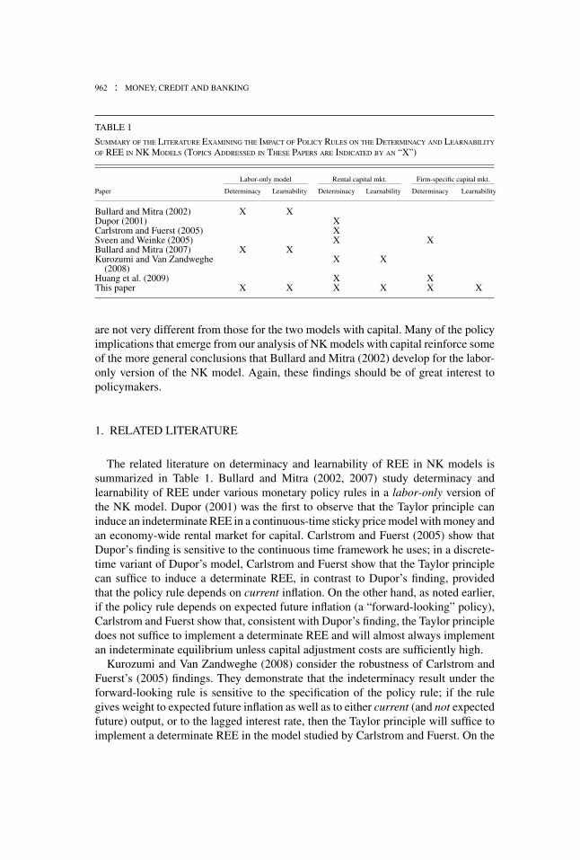
TABLE 1

SUMMARY OF THE LITERATURE EXAMINING THE IMPACT OF POLICY RULES ON THE DETERMINACY AND LEARNABILITY

OF REE IN NK MODELS (TOPICS ADDRESSED IN THESE PAPERS ARE INDICATED BY AN “X”)

Labor-only model Rental capital mkt. Firm-specific capital mkt.

Paper Determinacy Learnability Determinacy Learnability Determinacy Learnability

Bullard and Mitra (2002) X XDupor (2001) XCarlstrom and Fuerst (2005) XSveen and Weinke (2005) X XBullard and Mitra (2007) X XKurozumi and Van Zandweghe X X

(2008)Huang et al. (2009) X XThis paper X X X X X X

are not very different from those for the two models with capital. Many of the policyimplications that emerge from our analysis of NK models with capital reinforce someof the more general conclusions that Bullard and Mitra (2002) develop for the labor-only version of the NK model. Again, these findings should be of great interest topolicymakers.

1. RELATED LITERATURE

The related literature on determinacy and learnability of REE in NK models issummarized in Table 1. Bullard and Mitra (2002, 2007) study determinacy andlearnability of REE under various monetary policy rules in a labor-only version ofthe NK model. Dupor (2001) was the first to observe that the Taylor principle caninduce an indeterminate REE in a continuous-time sticky price model with money andan economy-wide rental market for capital. Carlstrom and Fuerst (2005) show thatDupor’s finding is sensitive to the continuous time framework he uses; in a discrete-time variant of Dupor’s model, Carlstrom and Fuerst show that the Taylor principlecan suffice to induce a determinate REE, in contrast to Dupor’s finding, providedthat the policy rule depends on current inflation. On the other hand, as noted earlier,if the policy rule depends on expected future inflation (a “forward-looking” policy),Carlstrom and Fuerst show that, consistent with Dupor’s finding, the Taylor principledoes not suffice to implement a determinate REE and will almost always implementan indeterminate equilibrium unless capital adjustment costs are sufficiently high.

Kurozumi and Van Zandweghe (2008) consider the robustness of Carlstrom andFuerst’s (2005) findings. They demonstrate that the indeterminacy result under theforward-looking rule is sensitive to the specification of the policy rule; if the rulegives weight to expected future inflation as well as to either current (and not expectedfuture) output, or to the lagged interest rate, then the Taylor principle will suffice toimplement a determinate REE in the model studied by Carlstrom and Fuerst. On the


other hand, Huang et al. (2009) show that Kurozumi and Van Zandweghe’s (2008)finding is sensitive to whether the elasticity of labor supply is assumed to be infinite (asKurozumi and Van Zandweghe 2008 assume) or is at a finite and empirically plausiblelevel, in which case indeterminacy remains a problem. However, they go on to showthat if the model involves both sticky prices and sticky wages then forward-lookingrules that also condition on current output or lagged interest rates generally serve toimplement determinate RE equilibria. The latter finding applies in economies witheither an economy-wide rental market for capital or a firm specific capital market.

Kurozumi and Van Zandweghe (2008) also briefly investigate whether learning (E-stability) might provide a remedy to the indeterminacy problem under the forward-looking rule studied by Carlstrom and Fuerst (2005) when no weight is given toeither current output or to the lagged interest rate and there are no capital adjustmentcosts. When equilibrium is indeterminate, there will be many rational expectationssolutions; the general solution form will allow for nonfundamental “sunspot” vari-ables to matter. In an effort to resolve the indeterminacy problem, Kurozumi and VanZandweghe suppose that agents are boundedly rational and make use of a funda-mental or “minimal state variable” solution that does not condition on any sunspotvariables; such solutions are just one (of many) possible solution representationswhen the REE is indeterminate. They show that, using such a rule, agents will learnthe REE but only under conditions that also satisfy the Taylor principle, that is, ifthe weight attached to future expected inflation is sufficiently greater than 1. Underthese assumptions, a sunspot-free REE can be reached, as long as rational agents arereplaced with adaptive learners.

Our findings for the NK model with an economy-wide rental market for capital (theenvironment studied by Carlstrom and Fuerst 2005, Kurozumi and Van Zandweghe2008, Huang et al. 2009) differ from these earlier findings in several important re-spects. First, we consider a wider variety of monetary policy rules than these papersconsider; in particular, the policy rules considered by Carlstrom and Fuerst (2005),Kurozumi and Van Zandweghe (2008), and Huang et al. (2009) all involve future ex-pected or current inflation whereas we also consider rules that involve lagged inflationor current expectations of inflation; the latter two rules are operationalizable in thesense of McCallum (1999) and may therefore be of greater interest and relevance topolicymakers. Second, our learning analysis is restricted to REE that are determinateor locally unique under the given policy rule and we suppose that agents use funda-mental, MSV solutions in an effort to learn REE; the minimal state variable (MSV)solutions are more appropriate in the case where REE is determinate as in that case,solutions that condition on nonfundamental sunspot variables cannot comprise REsolutions. Determinacy of equilibrium does not guarantee stability under learning andso it is important to check that determinate equilibria are also learnable as we do inthis paper. By contrast as noted earlier, Kurozumi and Van Zandweghe primarily uselearning dynamics as a means of resolving the indeterminacy of equilibrium problem.Summarizing, our analysis focuses attention on REE that are both determinate andlearnable as these are the equilibrium properties that should be of greatest interest topolicymakers.


The discrete-time models of Carlstrom and Fuerst (2005) and Kurozumi and VanZandweghe (2008) suppose there is an economy-wide rental market for capital. Asnoted in the introduction, Sveen and Weinke (2005) consider a discrete time versionof the NK model without money but with firm-specific capital and convex capitaladjustment costs. They show that this model is conceptually similar to the rentalmarket for capital NK model—the key difference lies in the parameterization of theNK Phillips curve. However they go on to show that in the firm-specific capital NKmodel, the Taylor principle does not suffice to ensure determinacy of REE under apolicy rule that responds to current inflation only. This finding stands in contrast toCarlstrom and Fuerst’s findings for the NK model with a rental market for capital.Sveen and Weinke show that interest rate rules that respond to both current inflationand output or that involve some policy smoothing are better able to induce determinateREE than is an interest rate rule that responds only to current inflation. Huang et al.(2009) generalize these findings to settings where there is disutility from labor supply,both price and wage stickiness and habit persistence in preferences for consumption.Neither of these papers consider the learnability (E-stability) of REE in the NK modelwith firm-specific capital; another novelty of our paper is that we do explore this issue.

A general impression of this literature is that in NK models with capital, the Taylorprinciple does not suffice to insure determinacy of REE. However, much less is knownabout E-stability of the REE of these models; with the exception Kurozumi and VanZandweghe (2008), no authors have explored the learnability of REE in NK modelswith capital, and the case of firm-specific capital has not been previously considered.1

More generally, comparisons of determinacy and learnability results between modelswith and without capital (labor-only) have not been made and there is not muchconsistency in the choice of interest rate rules and model calibrations used acrossstudies. In this paper, we provide a thorough and consistent analysis of determinacyand learnability of REE in three versions of the NK model—the first-generation labor-only models and the second-generation models with either a rental market for capitalor firm specific capital. In addition, we consider the five main interest rate rules thathave appeared in the literature: (i) a current data rule, (ii) a forward expectations rule,(iii) a lagged data rule, (iv) a contemporaneous expectations rule, and finally, (v) apolicy-smoothing rule. Many of our findings, for example, the E-stability of REE inNK models with firm-specific capital under the five policy rules we consider, are new.Some other findings, for example, for the labor-only model, are previously known,but in the latter case the value added of our paper lies in considering a consistentcalibration and set of policy rules across all model specifications (labor-only and thetwo models of capital).2 Our approach provides the reader with the clearest availablepicture to date of the conditions under which Taylor-type interest rate rules work toimplement determinate and learnable REE in the most commonly studied versions ofthe NK model of the monetary transmission mechanism (with or without capital).

1. Xiao (2008) also considers learnability of REE in an NK model with capital, but one that involvesincreasing returns in production.

2. Our analysis thus extends and encompasses that of Bullard and Mitra (2002, 2007).


2. A NEW KEYNESIAN MODEL WITH CAPITAL

2.1 The Environment

We consider two different environments that differ in their treatment of capital.Our benchmark model is one involving an economy-wide rental market for capital.The alternative model has firm-specific capital. The labor-only model is shown to bea special case of these two models.

Rental market for capital. The economy is composed of a large number of infinitelylived consumers. Each consumes a final consumption good Ct, and supplies laborNt. Savings can be held in the form of bonds Bt, or capital Kt. Consumers seek tomaximize expected, discounted life-time utility:

E0

∞∑t=0

β t

[C1−σ

t

1 − σ− N 1+χ

t

1 + χ

],

where σ , χ > 0 and 0 < β < 1. The budget constraint is given by

Ct + Bt

Pt+ It = Wt

PtNt + Rt

PtKt + (1 + it−1)

Bt−1

Pt+ Dt , (1)

where Pt and it denote the time t price level and nominal interest rate and investment,

It = I

(Kt+1

Kt

)Kt . (2)

The consumer’s sources of income are its real labor income (Wt/Pt)Nt, its realcapital rental income (Rt/Pt)Kt, its real return on one-period bonds Bt−1 purchased inperiod t − 1 and earning a gross nominal return of 1 + it−1, and its dividends fromownership of firms, Dt. The consumers allocate this income among consumption Ct,new bond purchases Bt/Pt, and new investment It. To allow comparisons betweenthis environment and the one with firm specific capital (described below), we followWoodford (2003) and suppose that each firm faces capital adjustment costs. Denotethese costs by I ( Kt+1

Kt), where the function I(·) is assumed to satisfy the steady-

state conditions: I(1) = δ, I′(1) = 1, and I′′(1) = εψ . Here, 0 < δ < 1 denotesthe depreciation rate and εψ > 0 characterizes the curvature of the adjustment costfunction.3

The first-order conditions for the consumer’s problem can be written as:

Nχt = C−σ

t

Wt

Pt, (3)

3. The parameter εψ has been interpreted as the elasticity of the investment/capital ratio with respectto Tobin’s q, in the steady state.


C−σt = βEt C

−σt+1

Pt

Pt+1, (4)

1 = βEt

(Ct+1

Ct

)−σ Pt

Pt+1(1 + it ), (5)

d It

d Kt+1= βEt

(Ct+1

Ct

)−σ (Rt+1

Pt+1− d It+1

d Kt+1

). (6)

There exists a continuum of monopolistically competitive firms producing differ-entiated intermediate goods. The latter are used as inputs by perfectly competitivefirms producing the single final good.

The final good is produced by a representative, perfectly competitive firm with aconstant returns to scale technology

Yt =(∫ 1

0Y

ε−1ε

j t d j

) εε−1

, (7)

where Yjt is the quantity of intermediate good j used as an input and ε > 1 governs theprice elasticity of individual goods. Profit maximization yields the demand schedule

Y jt =(

Pjt

Pt

)−ε

Yt , (8)

which, when substituted back into (7), yields

Pt =(∫ 1

0P1−ε

j t d j

) 11−ε

. (9)

The intermediate goods market features a large number of monopolistically com-petitive firms. The production function of a typical intermediate goods firm is:

Y jt = K αj t N 1−α

j t , (10)

where Kjt and Njt represent the capital and labor services hired by firm j.These firms’ real marginal cost ϕjt is derived by minimizing costs:

ϕ j t = 1

(1 − α)

Wt

Pt

N jt

Y jt= 1

α

Rt

Pt

K jt

Y jt. (11)

From this we can derive the expression

K jt

N jt= α

1 − α

Wt

Rt, (12)

which implies that the capital–labor ratio is equalized across firms, as is marginalcost itself.


Intermediate firms set nominal prices in a staggered fashion, according to thestochastic time dependent rule proposed by Calvo (1983). Each firm resets its pricewith probability 1 − ω each period, independent of the time that has elapsed since thelast price adjustment and does not reset its price with probability ω. A firm resettingits price in period t seeks to maximize:

Et

∞∑i=0

ωiβ i

(Ct+i

Ct

)−σ (P∗

t

Pt+iY jt+i − ϕ j t+i Y jt+i

), (13)

where P∗t represents the (common) optimal price chosen by all firms resetting their

prices in period t. This maximization problem yields the first-order condition,

Et

∞∑i=0

ωiβ i

(Ct+i

Ct

)−σ

Y jt+i

(P∗

t

Pt+i− ε

ε − 1ϕt+i

)= 0. (14)

The equation describing the dynamics for the aggregate price level is

Pt = [ωP1−ε

t + (1 − ω)P∗1−εt

] 11−ε . (15)

Finally, market clearing in the factor and goods markets implies that: Nt = ∫10 Njt

dj, Kt = ∫10 Kjt dj, Yt = ∫

10 Yjt dj, and Ct + It = Yt.

Firm-specific capital. Woodford (2003a, 2005) proposes a different version of the NKmodel in which an economy-wide rental market for capital does not exist. Instead,firms are assumed to accumulate capital for their own use only. This assumptionimplies that a firm’s price-setting decision is no longer separate from its capitalaccumulation decision (as it is in the rental market case), and this change leads toimportant changes in the dynamics of the NK model with capital. The main advantageof the firm-specific approach to capital accumulation is that it does not require anunrealistically high degree of price stickiness to match empirical facts relative tothe NK model with economy-wide rental markets that was examined in the previoussection.

With firm-specific capital, the model needs to be modified as follows. First, theconsumer’s budget constraint (1) is restated as

Ct + Bt

Pt= Wt

PtNt + (1 + it−1)

Bt−1

Pt+ Dt . (16)

That is, consumers no longer make investment decisions given the absence of anyeconomy-wide capital market.

Second, the firm’s problem is now defined as

max∞∑

i=0

β i

(Ct+i

Ct

)−σ (Pjt+i

Pt+iY jt+i − Wt+i

Pt+iN jt+i − I jt+i

)(17)


subject to constraints (8), (10), where firm-specific investment is given by

I jt = I

(K jt+1

K jt

)K jt . (18)

Notice that investment demand (18) is in the same form as (2) (i.e., it involves thesame convex adjustment function I(·)), but here it is firm specific. Note also thatPjt+i+1 = Pjt+i with probability ω.

Most first-order conditions, such as (3), (4), and (5), continue to hold in the NKmodel with firm-specific capital. However, three differences between this setup andthe rental-market setup will eventually lead to differences in the dynamics of themodel.

First, the first-order condition associated with capital is different in the firm-specificcapital model than in the rental market for capital model (cf. (6)). Maximizing (17)with respect to capital yields:

d I jt

d K jt+1= βEt

(Ct+1

Ct

)−σ (M Sjt+1

Pt+1− d It+1

d Kt+1

), (19)

where MSjt+1 denotes the nominal reduction in firm i’s labor cost associated withhaving an additional unit of capital in period t + 1, and is derived from the firm’smaximization problem as

MSjt = WtMPKjt

MPLjt, (20)

where MPK and MPL represent firm j’s marginal product of capital and of labor,respectively.

Second, marginal cost is now derived from the firm’s maximization problem as

ϕ j t = Wt/Pt

MPLjt.

The critical feature here is that marginal costs are no longer equalized across firms.They depend on each firm’s specific level of capital and labor.

Third, the first-order condition associated with Pjt+i looks identical to (14), butafter substituting in the expression for marginal cost, pricing decisions become afunction of firm-specific capital. Since a firm’s marginal cost is affected by its currentand future capital levels, its pricing decisions must also depend on its current andfuture capital levels. Future capital levels, on the other hand, depend in turn on today’sprice and the future prices set by the firm. This complicated mechanism is absent inthe rental-market case. Woodford (2005) shows that a linearized inflation equationcan be computed by applying the method of undetermined coefficients; we adopt hismethod in our later analysis.

Labor only model. For comparison purposes, we also study a version of the model inwhich labor is the only input in production. Setting I = K = 0 in our benchmark case


will reduce the model to a generic, labor-only NK model. We assume production hasconstant returns to scale in labor:

Y jt = N jt .

The consumer’s budget constraint is the same as (16), and the economy-wideresource constraint is simply Yt = Ct. The key first-order conditions are (3), (4), (5),and (14).

2.2 Reduced Linear Systems

In the next three subsections we describe the system of linearized equations weuse in our analysis of the determinacy and E-stability of REE in each of the threemodels that we consider. We use lower case letters to denote percentage deviationsof a variable from its steady-state value.

Benchmark model: Rental market for capital. In the benchmark model with a rentalmarket for capital, there are six nondynamic equations and four dynamic equations.The first equation is the linearized version of the labor supply schedule (3):

χnt + σct = wt − pt . (21)

The second and third equations are the linearized versions of (11). We are interestedin the average level of marginal costs, which are given by

ϕt = nt + (wt − pt ) − yt , (22)

= kt + (rt − pt ) − yt . (23)

The fourth equation is the linearized production function

yt = αkt + (1 − α)nt . (24)

The first dynamic equation is the NK Phillips curve, which is derived by solvingthe firm’s dynamic price-setting problem and combining it with (15). This equationis given by


πt = βEtπt+1 + κϕt , (25)

where κ = (1−ω)(1−βω)ω

.The second dynamic equation is the linearized version of (6), which describes the

evolution of capital:

k+1 = βEt kt+2 + 1

εψ

{[1 − β(1 − δ)]Et (rt+1 − pt+1) − (it − Etπt+1)}. (26)

The third dynamic equation is the Euler equation (5), which can be linearized as

ct = Et ct+1 − 1

σ(it − Etπt+1). (27)

The last dynamic equation is the market clearing condition

yt = C

Yct + K

Y[kt+1 − (1 − δ)kt ], (28)

where C, I, and Y represent steady-state levels of consumption, investment, andoutput.

Finally, we add the interest rate rule and use the nondynamic equations to substituteout seven variables k∗

t = kt+1, wt − pt, rt − pt, xt, it, ϕt, and yt. The system becomesa four-dimensional linear difference equation system consisting of st = (ct, nt, kt,π t)′:

Et st+1 = Jst . (29)

Firm-specific capital. With firm-specific capital, the NK Phillips curve becomes

πt = βEtπt+1 + κ∗ϕt . (30)

This equation is similar to (25), but the parameter κ∗ differs from the parameter κ

in (25). Woodford (2005) develops an algorithm that utilizes the method of unde-termined coefficients to compute κ∗. Sveen and Weinke (2004) show that κ∗ can beapproximated by 1−α

1−α+αεκ . Since 0 < α < 1 is capital’s share of output and ε > 1

governs the price elasticity of individual goods, using Sveen and Weinke’s approxi-mation we have that κ > κ∗, so that inflation is less responsive to changes in marginalcosts in the firm specific model of capital as compared with the rental market modelof capital. That is, as Sveen and Weinke (2005) point out, for any given value of theCalvo sticky price parameter ω, prices will be stickier in the firm-specific model ofcapital than they will be in the rental market for capital model.

We compared Sveen and Weinke’s approximation for κ∗ with the results of applyingWoodford’s algorithm and we found almost no difference, even for our later sensitivity


analysis that departs in certain dimensions from Sveen and Weinke’s calibration.Nevertheless, in all our analysis we use Woodford’s method to directly compute κ∗.

The marginal return to capital can be derived from (20) as

mst = wt − pt + nt − kt ,

and the aggregate capital accumulation equation is a linearized version of (19):

k+1 = βEt kt+2 + 1

εψ

{[1 − β(1 − δ)]Et mst+1 − (it − Etπt+1)}.

As in the rental market for capital case, the model with firm-specific capital can bereduced to a four-dimensional linear system of expectational difference equationswith the same variables as in (29).

Labor-only model. The labor-only NK model can be reduced to the New KeynesianPhillips curve (NKPC) and the expectational IS curve,

πt = βEtπt+1 + (σ + χ )κyt ,

yt = Et yt+1 − 1

σ(it − Etπt+1),

together with the first-order condition (4). The model is closed by an interest ratepolicy rule.

2.3 Monetary Authority

The central bank sets the nominal interest rate it every period according to a simple,linear Taylor-type policy rule contingent on information about output and inflation.Following Bullard and Mitra (2002, 2007), we consider five variants of this interestrate rule. The first is the “contemporaneous data” rule:

it = τππt + τy yt , (31)

where τπ ≥ 0 and τ y ≥ 0, and it, π t and yt denote percentage deviations of theinterest rate, the inflation rate, and output from their steady-state values. Rule (31)is a version of Taylor’s original (1993) policy rule whereby the nominal interest ratechanges with changes in current inflation and output.4 The “Taylor principle” is thatinterest rate changes should be more than proportional to changes in inflation; in(31) this is captured by the restriction that τπ > 1. Note, however, that the Taylor

4. Taylor-type interest rate rules typically condition on inflation and output gaps, that is, deviations ofinflation from a target level and of output from potential output, rather than on the levels of these variablesby themselves. As the determinacy/learnability conditions of the systems we consider depend only on themagnitudes of the coefficients impacting on inflation and output levels, we choose to work with interestrate rules such as (31) (as well as the four other types of rules that follow) that condition on these levelsonly; of course, all of our findings will continue to apply to rules that condition on inflation and outputgaps.


principle is not to be confused with a Taylor rule (such as (31)) which is an equationrelating how the central bank’s interest rate target changes in response to realizationsof inflation, output, and possibly other variables.

A second Taylor-type policy rule that is commonly considered (e.g., by Clarida etal. 1999), is the “forward expectations rule”:

it = τπ Etπt+1 + τy Et yt+1, (32)

where policymakers use expectations of future inflation and output using informationavailable at time t to determine the current interest rate target.

Since current data for output and inflation may not be available at time t, some havesuggested restricting attention to the use of time t − 1 data on output and inflation inthe determination of the interest rate target. This consideration gives rise to the nexttwo rules we consider. The third rule is the “lagged data” rule, which may be seen asan alternative to the current data rule (31). It is given by

it = τππt−1 + τy yt−1. (33)

Similarly, the fourth rule we consider, the “contemporaneous expectations” rule maybe seen as an alternative to the forward expectations rule (32) and is given by

it = τπ Et−1πt + τy Et−1 yt , (34)

where policy depends on forecasts of output and inflation that are formed using dataavailable through time t − 1.

In addition to the above four rules, we also consider an interest rate smoothingrule, where the policymaker gives some weight ρ to past interest rates and remainingweight 1 − ρ to the predictions of an interest rate rule such as rules 1-4 given above.Policy-smoothing rules have been considered by Bullard and Mitra (2007) for thelabor-only model; results for the two models with capital have not been previouslyexamined.

3. METHODOLOGY AND CALIBRATION

3.1 General Methodology

We now turn to our analysis of the determinacy and E-stability of REE underthe three models and five different interest rate rules. When we study E-stabilityproperties, we focus only on REE that are determinate.5 We use the benchmark modelto explain our general methodology. Precise conditions for E-stability of equilibriumunder all policy rules considered in this paper are available from the authors onrequest.

5. For an analysis of the E-stability properties of indeterminate rational expectations equilibria, see,for example, Honkapohja and Mitra (2004) and Evans and McGough (2005).


The determinacy of REE is assessed by computing the eigenvalues of the system(29). Since there is only one predetermined variable kt and the system is of dimensionfour, the REE will be determinate in this case if the number of explosive roots is threeand the number of stable roots is one (Blanchard and Kahn 1980). If the number ofstable roots exceeds one, we have an indeterminate REE. If there is no stable root,the system is explosive.

To study adaptive learning, we rewrite the system as

bzzt + bkkt = dk Et kt+1 + dz Et zt+1, (35)

kt+1 = ezzt + ekkt , (36)

where the second equation is derived from the capital accumulation equation, whichdoes not involve any expectations and so does not need to be learned. We assume thatagents use the perceived law of motion (PLM)

zt = a1 + ψkt ,

kt = a2 + mkt ,

which is in the same form as the MSV RE solution. By contrast with RE, learningagents do not initially know the parameter vectors a1, a2, ψ , and m and must learnthese over time. Given the PLM, we calculate the forward expectations as

Et kt+1 = a2 + mkt ,

Et zt+1 = a1 + ψ Et kt+1 = a1 + ψa2 + ψmkt .

Substituting these expressions into (35), we obtain a T-mapping from (a1, a2, ψ , m)′

to the actual law of motion of the model. Following Evans and Honkapohja (2001),we say the REE is E-stable (learnable by adaptive agents) if the differential equation,d

dτ(a1, a2, ψ, m) = T (a1, a2, ψ, m) − (a1, a2, ψ, m), evaluated at the REE solution,

is stable. This condition requires that all eigenvalues of D[T(a1, a2, ψ , m) − (a1, a2, ψ ,m)] evaluated at the REE have real parts that are less than zero. Evans and Honkapohja(2001) provide conditions under which this differential equation approximates thelimiting behavior of the recursive algorithms that characterize adaptive agent learning.

It is worth pointing out that assumptions about the agents’ information set canbe crucial in assessing E-stability results. In the baseline case outlined earlier, weimplicitly assume that both the private sector and the central bank can observecurrent values of the variable kt. They use this information to obtain forecasts Etzt+1

and Etkt+1, which in turn determine the current values of zt. This assumption appliesin models using the current data rule or the forward expectation rule. However,this assumption is sometimes criticized as being unrealistic, since current data areusually not available to economic agents.6 An alternative assumption is to assume

6. The case with the current data rule is especially controversial. As pointed out by Bullard and Mitra(2002), it implies that the central bank has “superior information” in that it reacts to current values of ytand π t while the private sector does not possess such information.


TABLE 2

CALIBRATIONS USED IN OUR NUMERICAL ANALYSES, QUARTERLY FREQUENCY

Parameter Description Value

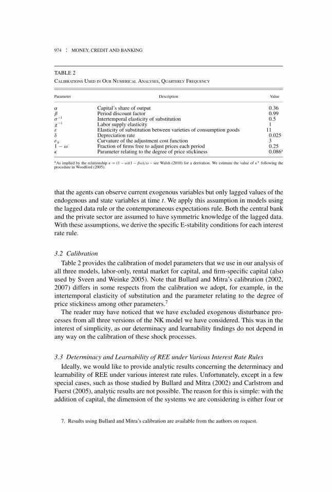
α Capital’s share of output 0.36β Period discount factor 0.99σ−1 Intertemporal elasticity of substitution 0.5χ−1 Labor supply elasticity 1ε Elasticity of substitution between varieties of consumption goods 11δ Depreciation rate 0.025εψ Curvature of the adjustment cost function 31 − ω Fraction of firms free to adjust prices each period 0.25κ Parameter relating to the degree of price stickiness 0.086a

aAs implied by the relationship κ = (1 − ω)(1 − βω)/ω – see Walsh (2010) for a derivation. We estimate the value of κ∗ following theprocedure in Woodford (2005).

that the agents can observe current exogenous variables but only lagged values of theendogenous and state variables at time t. We apply this assumption in models usingthe lagged data rule or the contemporaneous expectations rule. Both the central bankand the private sector are assumed to have symmetric knowledge of the lagged data.With these assumptions, we derive the specific E-stability conditions for each interestrate rule.

3.2 Calibration

Table 2 provides the calibration of model parameters that we use in our analysis ofall three models, labor-only, rental market for capital, and firm-specific capital (alsoused by Sveen and Weinke 2005). Note that Bullard and Mitra’s calibration (2002,2007) differs in some respects from the calibration we adopt, for example, in theintertemporal elasticity of substitution and the parameter relating to the degree ofprice stickiness among other parameters.7

The reader may have noticed that we have excluded exogenous disturbance pro-cesses from all three versions of the NK model we have considered. This was in theinterest of simplicity, as our determinacy and learnability findings do not depend inany way on the calibration of these shock processes.

3.3 Determinacy and Learnability of REE under Various Interest Rate Rules

Ideally, we would like to provide analytic results concerning the determinacy andlearnability of REE under various interest rate rules. Unfortunately, except in a fewspecial cases, such as those studied by Bullard and Mitra (2002) and Carlstrom andFuerst (2005), analytic results are not possible. The reason for this is simple: with theaddition of capital, the dimension of the systems we are considering is either four or

7. Results using Bullard and Mitra’s calibration are available from the authors on request.


five and too complicated to reduce to a system that would allow for analytic findings.This situation necessitates that we adopt a numerical approach. Still, to the extentpossible, we will try to provide some intuition for our numerical findings.8

Our approach is as follows. In all simulation exercises, we vary the weights τπ

and τ y, in the various interest rate rules. The ranges allowed for these weights coverall empirically relevant cases; in particular, we search over a fine grid of values forτπ between 0 and 5 and for τ y between 0 and 4. We use an increment stepsize of0.02. For each possible pair of weights [τπ , τ y] in this grid, we check whether theeigenvalues satisfy the conditions for (i) determinacy and (ii) E-stability. If the REEis indeterminate, we do not consider whether it is E-stable; such regions are simplylabeled “indeterminate” and are not shaded—the white or blank regions in the figuresbelow. If both conditions are satisfied, we indicate this in the figures below withsome shading and the label “determinate and E-stable.” If the REE is determinate butnot E-stable, we use a different shading and the label “determinate and E-unstable.”Finally, we use a different shading to indicate weight pairs for which all roots areexplosive (i.e., greater than one), and we label such regions “explosive.”

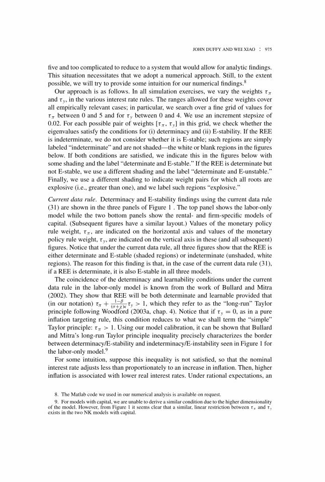
Current data rule. Determinacy and E-stability findings using the current data rule(31) are shown in the three panels of Figure 1 . The top panel shows the labor-onlymodel while the two bottom panels show the rental- and firm-specific models ofcapital. (Subsequent figures have a similar layout.) Values of the monetary policyrule weight, τπ , are indicated on the horizontal axis and values of the monetarypolicy rule weight, τ y, are indicated on the vertical axis in these (and all subsequent)figures. Notice that under the current data rule, all three figures show that the REE iseither determinate and E-stable (shaded regions) or indeterminate (unshaded, whiteregions). The reason for this finding is that, in the case of the current data rule (31),if a REE is determinate, it is also E-stable in all three models.

The coincidence of the determinacy and learnability conditions under the currentdata rule in the labor-only model is known from the work of Bullard and Mitra(2002). They show that REE will be both determinate and learnable provided that(in our notation) τπ + 1−β

(σ+χ)κ τy > 1, which they refer to as the “long-run” Taylorprinciple following Woodford (2003a, chap. 4). Notice that if τ y = 0, as in a pureinflation targeting rule, this condition reduces to what we shall term the “simple”Taylor principle: τπ > 1. Using our model calibration, it can be shown that Bullardand Mitra’s long-run Taylor principle inequality precisely characterizes the borderbetween determinacy/E-stability and indeterminacy/E-instability seen in Figure 1 forthe labor-only model.9

For some intuition, suppose this inequality is not satisfied, so that the nominalinterest rate adjusts less than proportionately to an increase in inflation. Then, higherinflation is associated with lower real interest rates. Under rational expectations, an

8. The Matlab code we used in our numerical analysis is available on request.9. For models with capital, we are unable to derive a similar condition due to the higher dimensionality

of the model. However, from Figure 1 it seems clear that a similar, linear restriction between τπ and τ yexists in the two NK models with capital.


FIG. 1. Determinacy and E-Stability Results under the Current Data Rule.

increase in Etπ t+1 or under learning, an upward departure of inflation forecasts fromrational expectations values is associated with a lower real interest rate and an increasein the output gap, yt, via the expectational IS equation, which serves in turn to ratifythe increase in π t via the NKPC. Under rational expectations the increase in Etπ t+1

is self-fulfilling, while under learning there is no mechanism to reverse a departure ofexpectations from rational expectations: the higher realization of inflation will leadagents to adjust their next forecast of inflation still higher.

The coincidence of the determinacy and learnability results under the current datarule in the NK models with a rental or firm-specific approach to capital is a new findingof this paper. For both models, the intuition is similar to that given for the labor-onlymodel, though deriving a meaningful analytic condition such as the long-run Taylorprinciple is not possible in NK models with capital given the greater dimensionsof those models.10 For the firm-specific capital model, while determinacy implieslearnability, we also observe that the “simple” Taylor principle, τπ > 1, no longer

10. Kurozumi and Van Zandweghe (2008) provide a similar Taylor-principle type analytic conditionfor determinacy (but not learnability) of REE in the rental-market model of capital, though their conditionsare derived under an interest rate rule that gives weight to future expected inflation, Etπ t+1, and to current


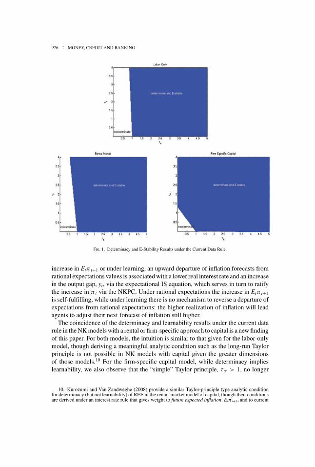
FIG. 2. Blown-Up View of the Indeterminate and E-unstable Region of the Firm-Specific Model of Capital under theCurrent Data Rule.

suffices to insure that the REE is determinate. Notice that in the firm-specific capitalmodel (bottom right panel of Figure 1), there is a very small “sliver” where τ y ≈ 0and τπ > 1, where the REE is both indeterminate and unstable under learning. Whilethis sliver may seem inconsequential in our figure, in the case of policy rules thatcondition only on inflation (τ y = 0) this region is a very plausible range for inflationresponses and is therefore a very important region of the parameter space to consider.

Figure 2 provides a blown-up view of this region. The presence of this region ofindeterminacy is consistent with Sveen and Weinke’s (2005) findings under a currentdata rule that gives zero weight to output [τ y = 0]. Indeed, they report that for variousvalues of ω, measuring the stickiness of prices (which include our calibrated valueω = 0.75), the Taylor principle may not suffice to guarantee determinacy of the REEunless sufficient weight is given either to real activity or to lagged interest rates (asin a policy-smoothing rule).

The intuition for the difference between the rental market and firm specific capitalcases must lie with the different parameterizations of the NKPC (25) and (30) since, asSveen and Weinke (2005) note, this is the only difference between the two linearizedversions of the models with capital. Recall that the difference between these twoNKPC equations lies in the coefficient on marginal costs ϕt, that is, κ in the rental

output (or its components consumption, investment)—a hybrid rule that differs from the current data rule(31) that we consider here.


market case and κ∗, in the firm-specific case, with κ > κ∗. Why is this the case?In the case of firm-specific capital, an increase in the demand for a firm’s outputwill raise the firm’s marginal costs, but as these are specific to the firm it will notaffect the marginal costs of other firms. Thus, in the firm-specific model, a firm thatis experiencing increased demand (and is free to adjust prices) will take into accountthe impact of price changes on its future relative demand and adjust prices less than itwould in the rental market model where changes in marginal costs are homogeneousacross all firms. The resulting decline in the firm’s future relative demand leads to afall in its future relative marginal cost as well, which reinforces the incentive to avoida large price increase today. Consequently, price setting is more forward looking(and will appear to be much more sluggish) in the firm-specific case relative to theeconomy-wide rental market case, where capital is perfectly mobile across firmsmaking the marginal costs firms face independent of the demand for their output.

To see why stickier price adjustment might lead to indeterminacy under the currentdata rule, consider whether an exogenous (sunspot driven) investment boom couldbe self-fulfilling. The answer depends on how it affects current and future marginalcosts and inflation and on how capital is modeled. Under a rental market for capital,the increase in investment demand will immediately drive up the marginal coststhat all firms face and via the NKPC, will increase current inflation. An activistmonetary policy focused on current inflation only (τπ > 1, τ y = 0) responds tothe increase in current inflation by raising interest rates, thereby, killing off thespeculative investment boom. By contrast, under a firm-specific model of capitalbecause investment is firm specific, price setting is more strategic (forward looking)with the result that price adjustment (by those firms free to adjust prices) is moresluggish. An increase in investment will raise marginal costs, but the impact oninflation will be reduced relative to the rental market case for the reasons given earlier.Furthermore, in the firm-specific model, the increase in firm-specific investment willlead to lower, future firm-specific marginal costs, lower future inflation, and hencelower future real interest rates, and with the more forward-looking view of firmsmaking firm-specific investments, this can serve to make the investment boom self-fulfilling. Note that this indeterminacy possibility would be reduced, if not eliminated,if monetary policy also put some weight on current output, as the investment boomwould increase yt and lead to an even higher increase in current interest rates.

Alternatively put, for the baseline calibration we use, ω = 0.75, prices will besufficiently flexible in the rental market model of capital to avoid the indetermi-nacy outcome when the Taylor principle holds, but the same will not be true in thefirm-specific model of capital.11 As we shall see, this same “sliver of a region” ofindeterminacy/E-instability in the firm-specific capital model can also arise underall four of the interest rate rules we consider that do not involve policy smoothing.

11. For calibrations other than the one we consider, for example, higher, but empirically implausiblevalues for ω, the small sliver of indeterminacy we observe for the firm-specific model of capital under thecurrent data rule when τ y ≈ 0 will also appear in the rental market model of capital under the current datarule so that the Taylor principle will not suffice to insure determinacy and learnability of REE for suchcalibrations.


Adding some policy inertia may work to eliminate this region of indeterminacy aswill be shown later in the paper.

Of course, a judicious (and empirically plausible) choice of policy rule weightswill also ensure that the REE is determinate and learnable in all three models under acurrent data rule. For instance, Taylor’s (1993) original calibration of the (current data)Taylor rule, adapted for the quarterly frequency of our calibrations, has τπ = 1.5 andτ y = 0.125.12 This calibration succeeds in implementing a determinate and learnableREE in all three models as Figures 1 and 2 confirm. The clear recommendation thatfollows from our findings using the current data rule is that the Taylor principle, intandem with some positive weight being given to real activity will reliably implementboth a determinate and learnable REE in models with capital.

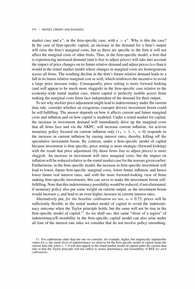
Aside from policy rule changes, we can also eliminate the sliver of indeterminacy inthe firm-specific capital model under the current data rule by assuming more flexibleprices, for example, values of ω that are closer to zero, which raises κ and hence κ∗.13

Alternatively, holding ω fixed, we can reduce α or ε or both, which will also increaseκ∗. The impact of such changes (higher values for κ∗) on the area of indeterminacyin the firm-specific model under the current data rule are shown in Figure 3, whereκ∗ is varied from 0.005 to 0.01 to 0.025 to 0.035. We see that for sufficiently highlevels of κ∗—our baseline calibration value is 0.012—the indeterminacy problem iseliminated.

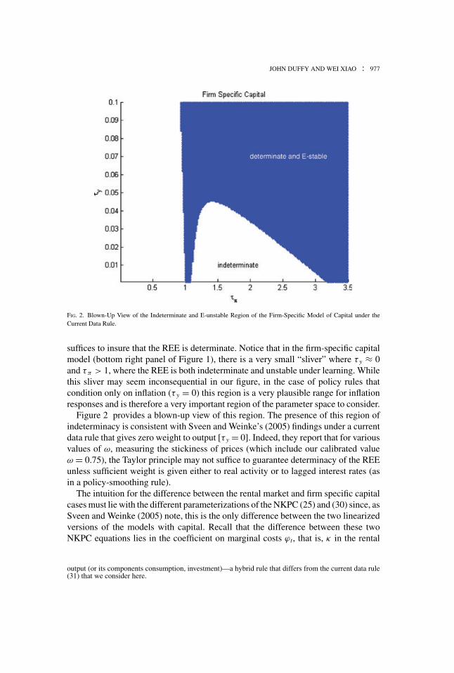
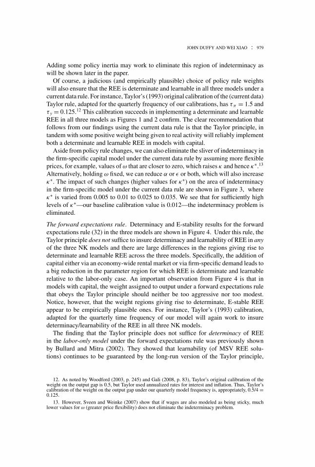
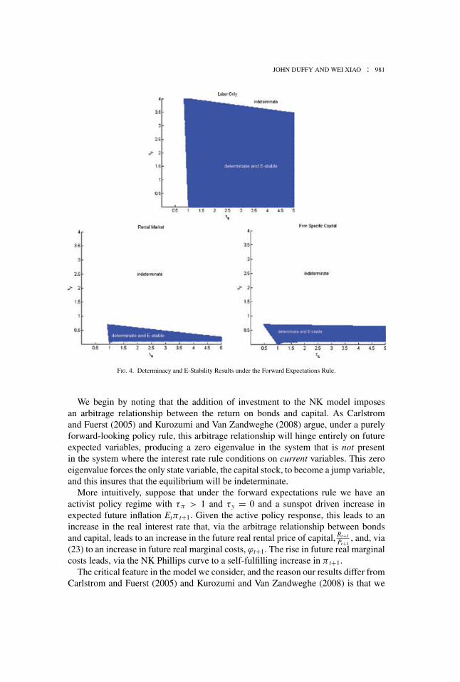
The forward expectations rule. Determinacy and E-stability results for the forwardexpectations rule (32) in the three models are shown in Figure 4. Under this rule, theTaylor principle does not suffice to insure determinacy and learnability of REE in anyof the three NK models and there are large differences in the regions giving rise todeterminate and learnable REE across the three models. Specifically, the addition ofcapital either via an economy-wide rental market or via firm-specific demand leads toa big reduction in the parameter region for which REE is determinate and learnablerelative to the labor-only case. An important observation from Figure 4 is that inmodels with capital, the weight assigned to output under a forward expectations rulethat obeys the Taylor principle should neither be too aggressive nor too modest.Notice, however, that the weight regions giving rise to determinate, E-stable REEappear to be empirically plausible ones. For instance, Taylor’s (1993) calibration,adapted for the quarterly time frequency of our model will again work to insuredeterminacy/learnability of the REE in all three NK models.

The finding that the Taylor principle does not suffice for determinacy of REEin the labor-only model under the forward expectations rule was previously shownby Bullard and Mitra (2002). They showed that learnability (of MSV REE solu-tions) continues to be guaranteed by the long-run version of the Taylor principle,

12. As noted by Woodford (2003, p. 245) and Gali (2008, p. 83), Taylor’s original calibration of theweight on the output gap is 0.5, but Taylor used annualized rates for interest and inflation. Thus, Taylor’scalibration of the weight on the output gap under our quarterly model frequency is, appropriately, 0.5/4 =0.125.

13. However, Sveen and Weinke (2007) show that if wages are also modeled as being sticky, muchlower values for ω (greater price flexibility) does not eliminate the indeterminacy problem.


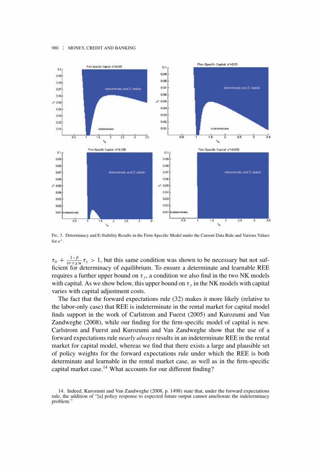
FIG. 3. Determinacy and E-Stability Results in the Firm-Specific Model under the Current Data Rule and Various Valuesfor κ∗.

τπ + 1−β

(σ+χ )κ τy > 1, but this same condition was shown to be necessary but not suf-ficient for determinacy of equilibrium. To ensure a determinate and learnable REErequires a further upper bound on τ y, a condition we also find in the two NK modelswith capital. As we show below, this upper bound on τ y in the NK models with capitalvaries with capital adjustment costs.

The fact that the forward expectations rule (32) makes it more likely (relative tothe labor-only case) that REE is indeterminate in the rental market for capital modelfinds support in the work of Carlstrom and Fuerst (2005) and Kurozumi and VanZandweghe (2008), while our finding for the firm-specific model of capital is new.Carlstrom and Fuerst and Kurozumi and Van Zandweghe show that the use of aforward expectations rule nearly always results in an indeterminate REE in the rentalmarket for capital model, whereas we find that there exists a large and plausible setof policy weights for the forward expectations rule under which the REE is bothdeterminate and learnable in the rental market case, as well as in the firm-specificcapital market case.14 What accounts for our different finding?

14. Indeed, Kurozumi and Van Zandweghe (2008, p. 1498) state that, under the forward expectationsrule, the addition of “[a] policy response to expected future output cannot ameliorate the indeterminacyproblem.”


FIG. 4. Determinacy and E-Stability Results under the Forward Expectations Rule.

We begin by noting that the addition of investment to the NK model imposesan arbitrage relationship between the return on bonds and capital. As Carlstromand Fuerst (2005) and Kurozumi and Van Zandweghe (2008) argue, under a purelyforward-looking policy rule, this arbitrage relationship will hinge entirely on futureexpected variables, producing a zero eigenvalue in the system that is not presentin the system where the interest rate rule conditions on current variables. This zeroeigenvalue forces the only state variable, the capital stock, to become a jump variable,and this insures that the equilibrium will be indeterminate.

More intuitively, suppose that under the forward expectations rule we have anactivist policy regime with τπ > 1 and τ y = 0 and a sunspot driven increase inexpected future inflation Etπ t+1. Given the active policy response, this leads to anincrease in the real interest rate that, via the arbitrage relationship between bondsand capital, leads to an increase in the future real rental price of capital, Rt+1

Pt+1, and, via

(23) to an increase in future real marginal costs, ϕt+1. The rise in future real marginalcosts leads, via the NK Phillips curve to a self-fulfilling increase in π t+1.

The critical feature in the model we consider, and the reason our results differ fromCarlstrom and Fuerst (2005) and Kurozumi and Van Zandweghe (2008) is that we


include capital adjustment costs in both versions of the NK model with capital.15

Capital adjustment costs make capital accumulation dependent on current and notjust future capital; this makes the arbitrage relationship not entirely forward lookingand works to eliminates the zero eigenvalue, which, in combination with a purelyforward-looking interest rate rule, will implement a determinate REE in certain cases,that is, with sufficiently high costs of adjustment.16

To see this more clearly, consider how the first-order condition, (6), changes if wedo not assume capital adjustment costs. In place of (2) we instead follow Carlstromand Fuerst (2005) and Kurozumi and Van Zandweghe (2008) and suppose that It =Kt+1 − (1 − δ)Kt. In that case, the first-order condition (6) is replaced by:

1 = βEt

(Ct+1

Ct

)−σ Pt

Pt+1(1 + it ). (37)

Combining (37) with (5) we have the arbitrage relationship:

(1 + it )

1 + πt+1= Rt+1

Pt+1+ 1 − δ, (38)

where for simplicity we have assumed perfect foresight. By contrast, under themodel with capital adjustment cost, the combination of first order conditions (6) and(5) yields a different arbitrage relationship (again under perfect foresight):

(1 + it )

1 + πt+1=

Rt+1

Pt+1− d It+1

d Kt+1

d It

d Kt+1

. (39)

Linearized versions of the two arbitrage conditions (38) and (39), which do notassume perfect foresight (respect expectations), are given by:

(it − Etπt+1) = [1 − β(1 − δ)] Et (rt+1 − pt+1), (40)

(it − Etπt+1) = [1 − β(1 − δ)] Et (rt+1 − pt+1) − εψ (βEt kt+2 − kt+1) , (41)

where kt+i = kt+i − kt. Notice that the only difference between (40) and (41) is theadditional right-hand-side term −εψ (βEt kt+2 − kt+1) in the latter. This additionalterm in (41) breaks the direct link between real interest rates and marginal costs that

15. The inclusion of capital adjustment costs is a standard practice in neoclassical investment theory.Carlstrom and Fuerst (2005) briefly discuss the addition of capital adjustment costs to the rental marketfor capital model they examine, and note that such adjustment costs may overturn their conclusions forforward-looking policy rules. However they consider a simpler, exponential form of capital adjustmentcosts. Kurozumi and Van Zandweghe (2008) do not consider capital adjustment costs.

16. An alternative mechanism for achieving the same end, as pursued by Kurozumi and Van Zandweghe(2008), is to have a hybrid policy rule that conditions on future expected inflation but on current output orits components (consumption, investment).


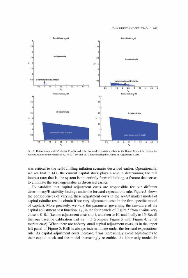
FIG. 5. Determinacy and E-Stability Results under the Forward Expectations Rule in the Rental Market for Capital forVarious Values of the Parameter εψ (0.1, 1, 10, and 15) Characterizing the Degree of Adjustment Costs.

was critical to the self-fulfilling inflation scenario described earlier. Operationally,we see that in (41) the current capital stock plays a role in determining the realinterest rate; that is, the system is not entirely forward looking, a feature that servesto eliminate the zero eigenvalue as discussed earlier.

To establish that capital adjustment costs are responsible for our differentdeterminacy/E-stability findings under the forward expectations rule, Figure 5 showsthe consequences of varying these adjustment costs in the rental market model ofcapital (similar results obtain if we vary adjustment costs in the firm-specific modelof capital). More precisely, we vary the parameter governing the curvature of thecapital adjustment cost function, εψ , in the four panels of Figure 5 from a value veryclose to 0–0.1 (i.e., no adjustment costs), to 1, and then to 10, and finally to 15. Recallthat our baseline calibration had εψ = 3 (compare Figure 5 with Figure 4, rentalmarket case). When there are no/very small capital adjustment costs, as in the upperleft panel of Figure 5, REE is always indeterminate under the forward expectationsrule. As capital adjustment costs increase, firms increasingly avoid adjustments totheir capital stock and the model increasingly resembles the labor-only model. In


FIG. 6. Determinacy and E-Stability Results under the Lagged Data Rule.

policy terms, the increase in capital adjustment costs also increases the upper boundon τ y that, together with the long-run Taylor principle condition, suffice to insuredeterminacy and learnability of REE under the forward expectations rule.

Figure 5 shows clearly that when εψ is close to zero, there are essentially noweight pairs for which the REE is both determinate and E-stable, consistent with thefindings of Carlstrom and Fuerst (2005) and Kurozumi and Van Zandweghe (2008)(e.g., compare the upper left panel of our Figure 5 with Figure 1 in Kurozumi andVan Zandweghe 2008). As εψ is steadily increased above zero, the determinacy/E-stability region increases as well, which is consistent with the intuition we haveprovided: the increasing convexity of adjustment costs means investment becomesboth more costly and more tied to the current level of the capital stock; as the lattervariable is predetermined, it makes the indeterminacy (and E-instability) outcomeless likely.

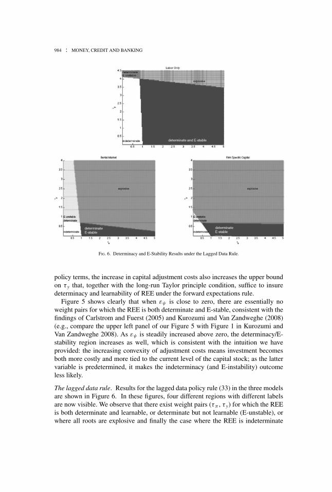
The lagged data rule. Results for the lagged data policy rule (33) in the three modelsare shown in Figure 6. In these figures, four different regions with different labelsare now visible. We observe that there exist weight pairs (τπ , τ y) for which the REEis both determinate and learnable, or determinate but not learnable (E-unstable), orwhere all roots are explosive and finally the case where the REE is indeterminate


(unshaded regions). The top panel of Figure 6 depicting the labor-only model, has anexpanded range of [τπ , τ y] pairs in order to reveal all four possibilities.

Under the lagged data rule we observe that in all three models, the simple Taylorprinciple [τπ > 1] does not suffice to insure both a determinate and learnable REE.This finding, for the labor-only model only, was earlier reported by Bullard and Mitra(2002); indeed, the labor-only case, (top panel of Figure 6) is as in Bullard and Mitra(2002, Figure 2). The novel finding we report under the lagged data rule is for the twomodels with capital: the determinate and learnable parameter regions in the modelswith capital are considerably smaller relative to the labor-only model (using our ownbaseline calibration) suggesting that a much more modest response to output is neededfor determinacy and learnability of REE. This finding is similar to what we foundunder the forward expectations rule; indeed, we have verified that for both modelswith capital, the upper bound on τ y increases with increases in capital adjustmentcosts (the graph is similar to Figure 5 and for this reason we do not show it here). Inthe firm-specific model of capital there is again a small sliver of indeterminate REEfor values of τ y that are close to 0 and values for τπ between 1 and 3.

Notice that the upper bound on τ y needed to ensure determinacy and learnability ofREE under the lagged data rule is to prevent REE from becoming locally explosive,that is, diverging away from the steady state and not from becoming indeterminate.However, the same transition from a determinate/learnable REE to an explosivesystem occurs under the labor-only model as shown by Bullard and Mitra (2002).Thus it seems that the addition of capital to the NK model is not the cause of thistransition in the dynamics of the system.

Notice further in Figure 6 that under the lagged data rule, determinate but E-unstable equilibria exist in all three models, but only for values of τπ < 1 andfor sufficiently large values of τ y, while for τπ < 1 and low values of τ y, REEis indeterminate. Similar findings using the lagged-data rule in the labor-only NKmodel were previously documented by Bullard and Mitra (2002), so again, our newdeterminacy and learnability findings for the two NK models with capital do notappear to result from adding capital to the system. Policy-based intuition for thesefindings is difficult to provide as determinacy of REE under the lagged policy rulecan obtain in all three models for all values of τπ (even τπ < 1) provided that τ y

lies in some narrow bands; for this reason, the lagged data rule may be undesirablefor practical use. On the other hand, we can claim that a necessary condition forE-stability of determinate REE under the lagged data policy rule is that some versionof the Taylor principle, for example, the simple version, τπ > 1, is satisfied.

Comparing the two different approaches to modeling capital, the firm-specificcase leads to a slightly larger region of determinate and learnable REE, though thefirm-specific case continues to have a sliver of a region where equilibrium is bothindeterminate and E-unstable. Nevertheless, for reasonable parameterizations of thelagged data version of the Taylor rule, for instance, Taylor’s original (1993) calibration(adapted to quarterly data) τπ = 1.5 and τ y = 0.125, determinacy and learnability ofthe REE are assured in all three models.


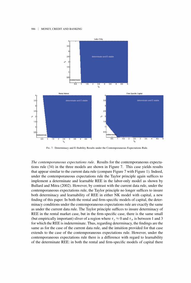
FIG. 7. Determinacy and E-Stability Results under the Contemporaneous Expectations Rule.

The contemporaneous expectations rule. Results for the contemporaneous expecta-tions rule (34) in the three models are shown in Figure 7. This case yields resultsthat appear similar to the current data rule (compare Figure 7 with Figure 1). Indeed,under the contemporaneous expectations rule the Taylor principle again suffices toimplement a determinate and learnable REE in the labor-only model as shown byBullard and Mitra (2002). However, by contrast with the current data rule, under thecontemporaneous expectations rule, the Taylor principle no longer suffices to insureboth determinacy and learnability of REE in either NK model with capital, a newfinding of this paper. In both the rental and firm-specific models of capital, the deter-minacy conditions under the contemporaneous expectations rule are exactly the sameas under the current data rule. The Taylor principle suffices to insure determinacy ofREE in the rental market case, but in the firm-specific case, there is the same small(but empirically important) sliver of a region where τ y ≈ 0 and τπ is between 1 and 3for which the REE is indeterminate. Thus, regarding determinacy, the findings are thesame as for the case of the current data rule, and the intuition provided for that caseextends to the case of the contemporaneous expectations rule. However, under thecontemporaneous expectations rule there is a difference with regard to learnabilityof the determinate REE: in both the rental and firm-specific models of capital there


is now a small sliver of a region where τ y is close to 0 and τπ is between 1 and 1.5(rental market) or between 1 and 3 (firm-specific) for which the REE is determinatebut is not E-stable (labeled “determinate and E-unstable” ). Thus, in the rental marketmodel under contemporaneous expectations, the Taylor principle may suffice for de-terminacy of REE but it no longer suffices for E-stability of REE. In the firm-specificmodel under the contemporaneous expectations rule, the region of determinate but Eunstable REE is a very small sliver (which is admittedly difficult to see) but whichlies along the border between the indeterminate (unshaded) and determinate and E-stable regions in Figure (7). We conjecture that the nonoverlap between determinacyand E-stability conditions must arise from the different timing of the information setused to form expectations under the contemporaneous expectations policy rule, aswe do not observe this kind of divergence under either the current data or forwardexpectations rules.

Of course, as Figure 7 shows, these regions of indeterminacy or E-instability canbe easily avoided by setting τ y sufficiently high. Indeed we observe that there is againa very wide range of plausible calibrations (e.g., Taylor’s 1993 calibration, τπ = 1.5and τ y = 0.125), which result in determinate and learnable REE in all three modelsunder the contemporaneous expectations rule.

Interest rate smoothing. Finally, we consider a policy rule involving interest ratesmoothing, that is, giving some weight to lagged values of the interest rate so thatpolicy does not adjust too quickly to changes in inflation or output. We focus on apolicy-smoothing version of the lagged interest rate rule (33) as given by:

it = ρit−1 + (1 − ρ)[τππt−1 + τy yt−1], (42)

where ρ ∈ (0, 1) is the weight given to the past interest rate target. Results forpolicy-smoothing versions of the other three rules we consider are broadly similar.We know from Bullard and Mitra (2007) that the addition of policy inertia in thelabor-only model can work to enlarge the region of policy weights for which a policyrule satisfying the Taylor principle yields determinate and learnable REE.

Here, in contrast to Bullard and Mitra (2007), we follow the convention in much ofthe literature on monetary policy rules (e.g., Rudebusch 2002) and imagine that theweight assigned to the lagged interest rate, it−1, and to the prescription of the policyrule [in square brackets] add up to unity; in this case the interest rate rule withoutsmoothing can be regarded as the special limiting case where ρ → 0. Woodford(2003b) has shown how such a “partial adjustment” model of monetary policy inertiamay result from optimizing behavior on the part of the central bank.17 Thus, we add

17. Some authors, for example, Rotemberg and Woodford (1998) and Giannoni and Woodford (2003),have derived optimal policy rules where the coefficient on the lagged interest rate is greater than 1.However, such a superinertial policy rule appears to be at odds with estimated interest rate rules. Forinstance, using U.S. data, Amato and Labauch (1999) estimate the current data rule (31) with the additionof a lagged interest rate (dependent) variable and report that the unrestricted coefficient estimate on thelagged interest rate is always less than one. While we think it would be of interest to consider superinertialinterest rate rules, a virtue of the partial adjustment model we examine is that it requires just one additional


FIG. 8. Determinacy and E-Stability Results under the Lagged Data Policy-Smoothing Rule.

the choice of ρ = 0.5 to our baseline calibration (Table 2) for the policy-smoothingrule (42) but we later explore the impact of changes in ρ.

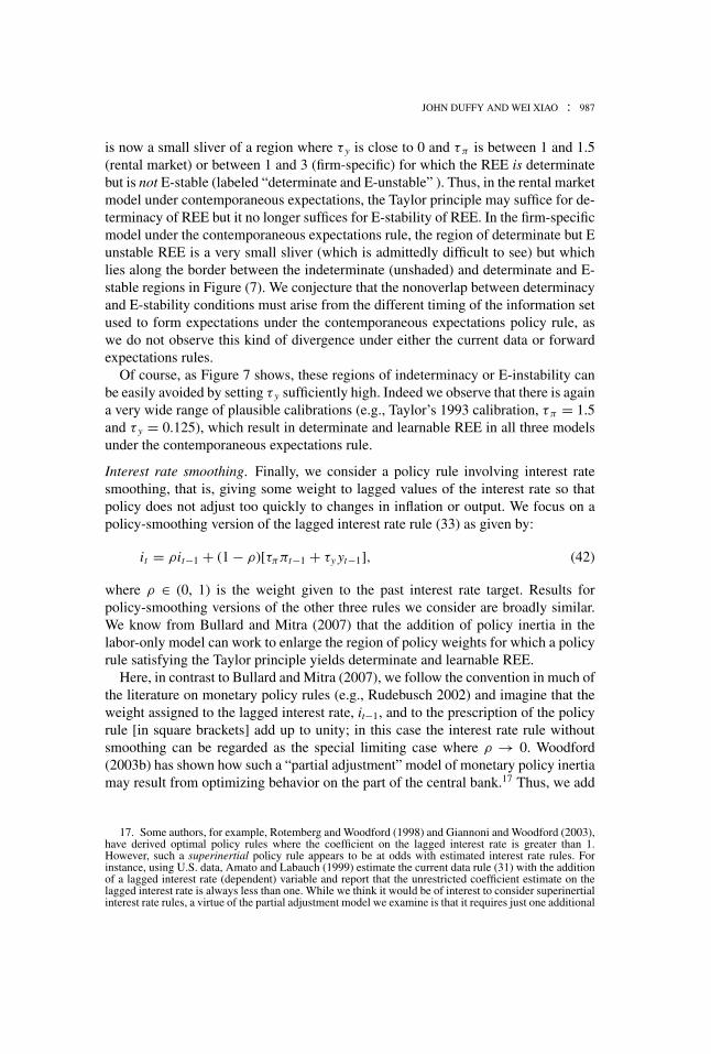
Determinacy and learnability results for the three models under the policy-smoothing rule (42) and our baseline calibration are shown in Figure 8. We seethat in this case, the Taylor principle suffices to guarantee both determinacy andlearnability of REE in the labor-only model but not in the two models that includecapital. Comparing Figure 8 with Figure 6, which showed results for the lagged datarule without inertia [ρ = 0], we observe that the addition of policy inertia [specifically,ρ = 0.5] greatly enlarges the range of policy weights for which REE are determinateand E-stable in both models with capital. Policy inertia acts like a positive weightattached to output and thus helps policymakers avoid indeterminacy and E-instability.As in the case of the other rules, one can find a large range of empirically plausiblevalues for the policy weights (τπ , τ y), for which the REE is both determinate andlearnable, for example, Taylor’s original calibration.

We also explore the sensitivity of our findings using the policy smoothing rule (42)to changes in the persistence parameter ρ. We focus on the rental market for capital

parameter, ρ, making it easier to see whether our findings without inertia generalize to the addition ofsome inertia.


FIG. 9. Sensitivity Analysis for the Rental Market Model under the Policy-Smoothing Rule (42) Showing How theDeterminate and E-stable Region Varies with Changes in the Value of ρ.

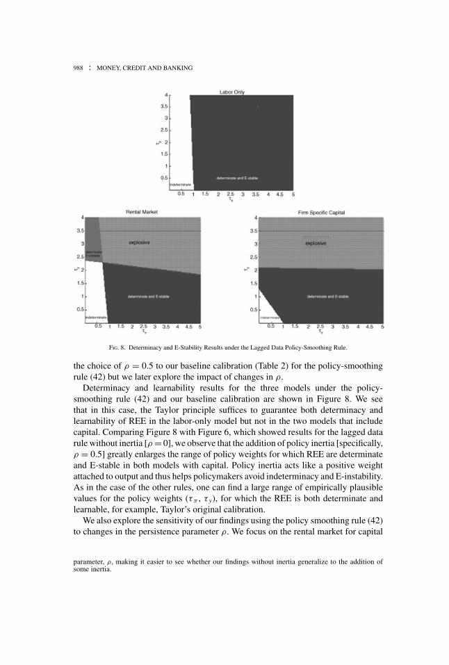
model as the results are similar for the firm-specific model of capital. Figure 9 revealsthat in the rental market for capital model, the region of weight pairs for which REE isboth determinate and E-stable increases as ρ increases. For instance, the determinateand E-stable polygon for the baseline ρ = 0.5 case in Figure 9 corresponds to thedeterminate and E-stable region of Figure 8. As ρ is lowered to 0.2, the upper boundto this determinate and E-stable region falls relative to the baseline case and as ρ israised to 0.75, the upper bound to the determinate and E-stable region rises relativeto the baseline case as Figure 9 illustrates. The main finding from this analysis isthat increasing persistence in policy [the value of ρ] in models with capital leadsto an expansion in the range of policy rule weights for which equilibrium is bothdeterminate and learnable.

4. CONCLUSIONS

We have studied determinacy and learnability of REE in three different NK models,one with labor only and two that add productive capital via an economy-wide rentalmarket for capital or via firm-specific demand for capital. The addition of capital tothe NK model allows for the study of investment decisions, an important componentof aggregate demand.


Determinacy and learnability are two highly desirable properties for REE and itshould be the aim of central banks to adopt interest rate policies that implement equi-libria possessing both of these properties. While Bullard and Mitra (2002, 2007) findthat the Taylor principle nearly always suffices for both determinacy and learnabilityof REE in the labor-only model, the addition of capital to the NK model requiressome further qualifications to this conclusion. In particular, we find that (i) in themodel with a rental market for capital, the Taylor principle continues to suffice toinsure both determinacy and learnability of REE if the interest rate rule responds tocurrent data on inflation and output. However, we also find (ii) the Taylor principleneed not suffice for both determinacy and learnability of equilibrium if the interestrate rule responds to future or contemporaneous expectations of inflation and outputor to lagged values of these variables or if the central bank uses a policy-smoothingrule. We further find (iii) that in the model with firm-specific capital the Taylorprinciple never suffices to insure both determinacy and learnability of REE for thecalibration we consider. Finally, (iv) an important policy finding is that the Taylorprinciple appears to be necessary, but not sufficient, for E-stability (learnability) ofdeterminate REE in all of the models that we consider.

While the Taylor principle does not suffice to guarantee determinacy and learn-ability of equilibrium, we can still reach several practical conclusions that shouldbe of interest to central bankers. First, while the specific findings for the labor-onlymodel do not generalize to models with capital and investment decisions, some ofthe policy recommendations for the labor-only model appear to carry over to modelsthat include capital. Specifically, two of the rules we consider, the current data ruleand the contemporaneous expectations rule, both of which are operational in thesense of McCallum (1999), fare the best in all three models in terms of admitting thelargest possible regions of determinate and learnable REE. Second, the results for thefirm-specific and rental models of capital suggest that there is high value to policyrules that obey both the Taylor principle and give some weight to output and/or topolicy smoothing so as to avoid indeterminacy and instability under learning. Undera forward-looking policy rule, the response to output should not be too modest nortoo aggressive, and under a policy-smoothing rule, the weight attached to past inter-est rates should not be too small. Finally, we note that some (τπ , τ y) pairs succeedin implementing determinate and learnable REE in all models and for all interestrate rules that we have considered. In particular, the parameterization proposed byTaylor (1993) adjusted for the quarterly frequency of our model,—τπ = 1.5 and τ y =0.125—belongs to that class. Perhaps the empirical success of Taylor’s (1993) policyrule rests as much with the policy weights he chose for that rule as with the principlethat also bears his name.

LITERATURE CITED

Amato, Jeffery D., and Thomas Labauch. (1999) “The Value of Interest Rate Smoothing:How the Private Sector Helps the Federal Reserve.” Federal Reserve Bank of Kansas CityEconomic Review, 84, 47–64.


Blanchard, Olivier J., and Charles M. Kahn. (1980) “The Solution of Linear Difference Modelsunder Rational Expectations.” Econometrica, 48, 1305–11.

Bullard, James. (2006) “The Learnability Criterion and Monetary Policy.” Federal ReserveBank of St. Louis Review, 88, 203–17.

Bullard, James, and Kaushik Mitra. (2002) “Learning about Monetary Policy Rules.” Journalof Monetary Economics, 49, 1105–29.

Bullard, James, and Kaushik Mitra. (2007) “Determinacy, Learnability, and Monetary PolicyInertia.” Journal of Money, Credit, and Banking, 39, 1177–1212.

Calvo, Guillermo A. (1983) “Staggered Prices in a Utility-Maximizing Framework.” Journalof Monetary Economics, 12, 383–98.

Carlstrom, Charles T., and Timothy S. Fuerst. (2005) “Investment and Interest Rate Policy: ADiscrete Time Analysis.” Journal of Economic Theory, 123, 4–20.

Clarida, Richard, Jordi Gali, and Mark Gertler. (1999) “The Science of Monetary Policy: ANew Keynesian Perspective.” Journal of Economic Literature, 37, 1661–1707.

Dupor, Bill. (2001) “Investment and Interest Rate Policy.” Journal of Economic Theory, 98,85–113.

Evans, George W., and Seppo Honkapohja. (2001) Learning and Expectations in Macroeco-nomics. Princeton, NJ: Princeton University Press.

Evans, George W., and Bruce McGough. (2005) “Stable Sunspot Solutions in Models withPredetermined Variables.” Journal of Economic Dynamics and Control, 29, 601–25.

Gali, Jordi. (2008) Monetary Policy, Inflation, and the Business Cycle. Princeton, NJ: PrincetonUniversity Press.

Giannoni, Marc P., and Michael Woodford. (2003) “How Forward-Looking Is Optimal Mon-etary Policy?” Journal of Money, Credit and Banking, 35, 1425–69.

Honkapohja, Seppo, and Kaushik Mitra. (2004) “Are Non-Fundamental Equilibria Learnablein Models of Monetary Policy?” Journal of Monetary Economics, 51, 1743–70.

Huang, Kevin X.D., Qinglai Meng, and Jianpo Xue. (2009) “Is Forward-Looking Inflation Tar-geting Destabilizing? The Role of Policy’s Response to Current Output under EndogenousInvestment.” Journal of Economic Dynamics and Control, 33, 409–30.

Kurozumi, Takushi, and Willem Van Zandweghe. (2008) “Investment, Interest Rate Policy andEquilibrium Stability.” Journal of Economic Dynamics and Control, 32, 1489–1516.

McCallum, Bennett T. (1999) “Issues in the Design of Monetary Policy Rules.” In Handbook ofMacroeconomics, vol. 1C, edited by John B. Taylor and Michael Woodford, pp. 1483–1530.Amsterdam: Elsevier.

Rotemberg, Julio J., and Michael Woodford. (1998) “An Optimization-Based EconometricFramework for the Evaluation of Monetary Policy: Expanded Version.” NBER TechnicalWorking Paper No. 233.

Rudebusch, Glenn D. (2002) “Term Structure Evidence on Interest Rate Smoothing and Mon-etary Policy Inertia.” Journal of Monetary Economics, 49, 1161–87.

Sveen, Tommy, and Lutz Weinke. (2004) “Pitfalls in the Modeling of Forward-Looking PriceSetting and Investment Decisions.” Norges Bank Working Paper No. 2004/1.

Sveen, Tommy, and Lutz Weinke. (2005) “New Perspectives on Capital, Sticky Prices, and theTaylor Principle.” Journal of Economic Theory, 123, 21–39.

Sveen, Tommy, and Lutz Weinke. (2007) “Firm-Specific Capital, Nominal Rigidities, and theTaylor Principle.” Journal of Economic Theory, 136, 729–37.


Taylor, John B. (1993) “Discretion versus Policy Rules in Practice.” Carnegie-RochesterConference Series on Public Policy, 39, 195–214.

Taylor, John B. (1999) “A Historical Analysis of Monetary Policy Rules.” In Monetary PolicyRules, edited by John B. Taylor, pp. 319–41. Chicago: University of Chicago Press.

Walsh, Carl E. (2010) Monetary Theory and Policy, 3rd ed. Cambridge, MA: MIT Press.

Woodford, Michael. (2001) “The Taylor Rule and Optimal Monetary Policy.” American Eco-nomic Review, 91, 232–37.

Woodford, Michael. (2003a) Interest and Prices. Princeton, NJ: Princeton University Press.

Woodford, Michael. (2003b) “Optimal Interest-Rate Smoothing.” Review of Economic Studies,70, 861–86.

Woodford, Michael. (2005) “Firm-Specific Capital and the New Keynesian Phillips Curve.”International Journal of Central Banking, 1, 1–46.

Xiao, Wei. (2008) “Increasing Returns and the Design of Interest Rate Rules.” MacroeconomicDynamics, 12, 22–49.

Documents

Investment and Monetary Policy: Learning and Determinacy