SPECTRAL NETWORKS AND NON-ABELIANIZATION FOR REDUCTIVEGROUPS

Matei Ionita

A DISSERTATION

in

Mathematics

Presented to the Faculties of the University of Pennsylvania in Partial Fulfillmentof the Requirements for the Degree of Doctor of Philosophy

2020

Supervisor of Dissertation

Ron DonagiProfessor of Mathematics

Co-Supervisor of Dissertation

Tony PantevClass of 1939 Professor of Mathematics

Graduate Group Chairperson

Julia Hartmann, Professor of Mathematics

Dissertation Committee:Ron Donagi, Professor of MathematicsTony Pantev, Class of 1939 Professor of MathematicsJustin Hilburn, Postdoctoral Fellow, University of Waterloo and Perimeter Institutefor Theoretical Physics

member:FF54C9FF-5112-4C05-835B-3C92768EAB0E 7FAC1D57-638F-4849-B3A6-A743B7A24B40

Digitally signed by member: FF54C9FF-5112-4C05-835B-3C92768EAB0E 7FAC1D57-638F-4849-B3A6-A743B7A24B40Date: 2020.05.04 16:40:45 -04'00'

Tony Pantev Digitally signed by Tony Pantev Date: 2020.05.04 16:57:16 -04'00'

JuliaHartmann

Digitally signed by Julia HartmannDate: 2020.05.04 17:08:36 -04'00'

Acknowledgments

I am heavily indebted and immensely grateful to many people, whose direct or indirect

contributions influenced this work, and my mathematical progress in general.

My advisors Ron and Tony introduced me to many fascinating mathematical objects

and questions, but also gave me the freedom to choose what to work on. Ron’s insistence

that I understand explicit examples before attempting to make sweeping statements led

to significant corrections, simplifications, and sometimes falsification of said statements.

I thank my collaborator Benedict for his work on our joint project, and more generally

for sharing his ideas about mathematics. He evangelized the benefits of cameral covers to

the rest of us (sometimes obstinate and reactionary) Penn math students; cameral covers

then turned out to be the essential starting point of our joint work. Benedict also taught

me that no moduli stack is too difficult to define, if you just use enough fiber products.

Most of the mathematics that I learned at Penn was in the seminars that I attended, in

which, aside from the nutritious mathematical content, I also learned to give talks which

were, I hope, progressively less disastruous. As postdocs, Mauro and Justin organized

the first of these seminars, and set a high bar for the next ones. Benedict and Sukjoo, as

my office-mates and the recurrent characters in all seminars, heavily influenced the way

ii

I think about mathematics. Other members of our group, such as Rodrigo, Michail, Jia

Choon, Ziqi and Marielle, contributed to my knowledge and enjoyment of math.

I would also like to thank the administrative staff in the Penn mathematics department

for their support and goodwill; Reshma, Monica, Paula and Robin have been constantly

helpful and kind.

My very decision to major in mathematics was influenced by the collective of students

with whom I studied at Columbia. My fate was sealed by two chance events: sitting

near Nilay and Yifei in an E&M class in first year, and then drawing a winning lot and

becoming Leo’s room-mate in second year. Ever since, I’ve been hoping that their fun

and proactive attitude towards math would rub off on me, if we hang out for long enough.

Whatever intellectual rigor and ambition I may have is due to my parents Diana and

Sorin. By explicit encouragement, and also by practicing what they preach, they taught

me the benefits of consistent, efficient work.

I thank my partner Andreea for embarking on the double adventure of a PhD and a

life abroad with me. Living with her and watching her work taught me how lazy I am

by comparison, and motivated me to do more. I’m grateful for her perennial curiosity

about my work, despite the fact that it contains even more technical mumbo-jumbo

than the average PhD thesis. Aside from Andreea’s unquantifiable emotional support,

I benefitted from her advice on structuring my thesis, delivering a good presentation,

constructing morphisms of Lie algebras, understanding positive roots in root systems of

type A, choosing a soundtrack for many frustrating hours of work, and much else.

Finally, I thank Andreea, Benedict and Nilay for the grunt work of reading an early

draft of this thesis and giving helpful suggestions.

iii

ABSTRACT

Spectral Networks and Non-Abelianization for Reductive Groups

Matei Ionita

Ron Donagi and Tony Pantev, Advisors

Non-abelianization was introduced in [16] as a way to study the moduli space of local

systems of n-dimensional vector spaces on a Riemann surface X. This thesis, which is

based on the forthcoming paper [23], explains how to generalize non-abelianization to the

setting of G-local systems, for any reductive Lie group G. The main tool used to achieve

this goal is a graph on X called a spectral network. These graphs have been introduced

in [16] for groups of type A, and extended in [27] to groups of type ADE. We construct

spectral networks for all reductive G, using a branched cover of X called a cameral

cover, which is, in general, different from the spectral cover used in previous work on the

subject. Our framework emphasizes the relationship between spectral networks and the

trajectories of quadratic differentials, which provides a strategy to prove genericity results

about spectral networks. Finally, we show how to associate, in an equivariant fashion,

unipotent automorphisms called Stokes factors to edges of a spectral network. We define

non-abelianization as a “cut and reglue” construction: we cut along the spectral network

and reglue using the Stokes factors. Our construction, unlike the one in [16], does not

rely on choices of trivializations for the local systems or for the branched cover.

iv

Contents

1 Introduction 1

1.1 Local systems and non-abelianization . . . . . . . . . . . . . . . . . . . . . 1

1.2 Quadratic differentials and spectral networks . . . . . . . . . . . . . . . . 9

1.3 Outline of the thesis . . . . . . . . . . . . . . . . . . . . . . . . . . . . . . 17

1.4 Conventions and notation . . . . . . . . . . . . . . . . . . . . . . . . . . . 18

2 Geometric background 20

2.1 Local systems . . . . . . . . . . . . . . . . . . . . . . . . . . . . . . . . . . 20

2.2 Higgs bundles . . . . . . . . . . . . . . . . . . . . . . . . . . . . . . . . . . 22

2.3 Spectral and cameral covers . . . . . . . . . . . . . . . . . . . . . . . . . . 26

3 Lie theoretic technicalities 32

3.1 Chevalley bases and sl2-triples . . . . . . . . . . . . . . . . . . . . . . . . 32

3.2 Scattering diagrams and Stokes factors . . . . . . . . . . . . . . . . . . . . 39

3.3 Explicit calculations for planar root systems . . . . . . . . . . . . . . . . . 57

4 Cameral and spectral networks 64

4.1 The WKB construction . . . . . . . . . . . . . . . . . . . . . . . . . . . . 64

v

4.2 How generic are WKB cameral networks? . . . . . . . . . . . . . . . . . . 81

4.3 Equivariance and spectral networks . . . . . . . . . . . . . . . . . . . . . . 89

5 The non-abelianization map 94

5.1 From T-local systems to N-local systems . . . . . . . . . . . . . . . . . . . 95

5.2 The S-monodromy condition . . . . . . . . . . . . . . . . . . . . . . . . . . 100

5.3 From N-local systems to G-local systems . . . . . . . . . . . . . . . . . . . 104

5.3.1 Equivariant assignment of Stokes factors . . . . . . . . . . . . . . . 111

vi

Chapter 1

Introduction

1.1 Local systems and non-abelianization

Given a Riemann surface X and a reductive Lie group G, the moduli space of local

systems LocG(X) is an important topological invariant of X, widely used in geometry and

physics. For example, if X is hyperbolic and G = PSL2(R), a certain subset of LocG(X)

can be identified with Teichmuller space, which parametrizes complex structures on X,

up to homeomorphisms isotopic to the identity. Moreover, LocG(X) can be identified

complex-analytically with the moduli space of principal G-bundles with flat connection.

In this guise they arise in physics, for example as classical solutions to Chern-Simons

theory.

Fixing a basepoint x ∈ X, we can regard LocG(X) as the space of group homomor-

phisms from the fundamental group of X to G, modulo conjugation by G:

LocG(X) ∼= Hom(π1(X,x), G

)/G. (1.1.1)

In the case of abelian groups, such as a torus T ∼= (C∗)n, the conjugation action of T

1

is trivial, and LocT (X) is a quotient of a product of copies of T by this trivial action.

For non-abelian G, it is harder to describe the effect of the quotient by the adjoint

action, and, consequently, the structure of LocG(X). The purpose of this thesis is to

construct “non-abelianization maps”, which, modulo some details, are morphisms from a

moduli space of T -local systems on a branched cover of X to LocG(X). Since T is abelian,

the structure of the source space is well understood, and we can use the non-abelianization

maps to probe the structure of the target space LocG(X).

Gaiotto, Moore and Neitzke first introduced non-abelianization for the cases G =

GL(n,C), G = SL(n,C) in the paper [16], which builds up on their work on the n = 2

case in [17]. They further explored this topic in [18], where they also made a con-

nection with the coordinates on LocG(X) constructed by Fock and Goncharov in [15].

Subsequently, other authors gave detailed constructions and new results in the cases

G = SL(2,C), SL(2,R); see [14], [21], [29]. The author of this thesis, in joint work with

Morrissey, generalize non-abelianization to arbitrary reductive G in the forthcoming paper

[23]. The results we present in this thesis are based on sections 3-5 of loc. cit.

The main results are theorems 1.1.4 and 1.1.5 below. Before stating them, we discuss

an example of non-abelianization in the case of GL(2,C), to provide the reader with some

intuition. For ease of exposition, in this example we work with the associated rank 2

vector bundles, rather than the GL(2,C)-principal bundles.

Example 1.1.1. Consider the double cover of the punctured affine line with a branch point

2

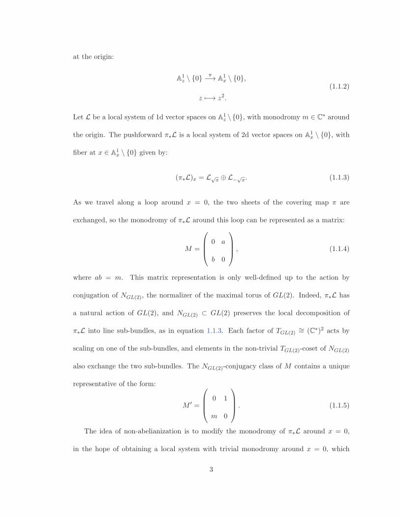
at the origin:

A1z \ {0} π−→ A1

x \ {0},

z �−→ z2.

(1.1.2)

Let L be a local system of 1d vector spaces on A1z \ {0}, with monodromy m ∈ C∗ around

the origin. The pushforward π∗L is a local system of 2d vector spaces on A1x \ {0}, with

fiber at x ∈ A1x \ {0} given by:

(π∗L)x = L√x ⊕ L−√

x. (1.1.3)

As we travel along a loop around x = 0, the two sheets of the covering map π are

exchanged, so the monodromy of π∗L around this loop can be represented as a matrix:

M =

⎛⎜⎜⎝ 0 a

b 0

⎞⎟⎟⎠ , (1.1.4)

where ab = m. This matrix representation is only well-defined up to the action by

conjugation of NGL(2), the normalizer of the maximal torus of GL(2). Indeed, π∗L has

a natural action of GL(2), and NGL(2) ⊂ GL(2) preserves the local decomposition of

π∗L into line sub-bundles, as in equation 1.1.3. Each factor of TGL(2)∼= (C∗)2 acts by

scaling on one of the sub-bundles, and elements in the non-trivial TGL(2)-coset of NGL(2)

also exchange the two sub-bundles. The NGL(2)-conjugacy class of M contains a unique

representative of the form:

M ′ =

⎛⎜⎜⎝ 0 1

m 0

⎞⎟⎟⎠ . (1.1.5)

The idea of non-abelianization is to modify the monodromy of π∗L around x = 0,

in the hope of obtaining a local system with trivial monodromy around x = 0, which

3

Figure 1.1: Trivalent graph with a unipotent automorphism associated to each edge.

would therefore extend to a local system on A1x. The modification is done by cutting and

re-gluing the local system along the edges of the trivalent graph W pictured in Figure

1.1. Concretely:

• consider the restriction π∗L|A1x\W ;

• re-glue this restriction across the edges of W, using an unipotent automorphism

called Stokes factor associated to each edge, as in Figure 1.1.

The resulting local system has monodromy around the origin:

M ′u+u−u+ =

⎛⎜⎜⎝ 0 1

m 0

⎞⎟⎟⎠⎛⎜⎜⎝ 1 1

0 1

⎞⎟⎟⎠⎛⎜⎜⎝ 1 0

−1 1

⎞⎟⎟⎠⎛⎜⎜⎝ 1 1

0 1

⎞⎟⎟⎠

=

⎛⎜⎜⎝ 0 1

m 0

⎞⎟⎟⎠⎛⎜⎜⎝ 0 −1

1 0

⎞⎟⎟⎠

=

⎛⎜⎜⎝ 1 0

0 −m

⎞⎟⎟⎠ .

(1.1.6)

4

In the particular case m = −1, we obtain a local system which extends to all of A1x; we

call this the non-abelianization nonab(L) of the original L. The terminology is motivated

by the passage from the abelian structure group GL(1,C) to the non-abelian structure

group GL(2,C). The situation is summarized in the following diagram.

LocVect1d(A1z \ {0}) LocVect2d(A

1x \ {0}) LocVect2d(A

1x \ {0})

Locm=−1Vect1d

(A1z \ {0}) LocVect2d(A

1x)

π∗ reglue

nonab

(1.1.7)

Remark 1.1.2. Equation 1.1.6 above is a calculation performed with matrices, but a more

rigorous approach would involve working with NGL(2)-conjugacy classes. In section 5.3.1,

we will show how to map the monodromy of N -local systems to Stokes factors in an N -

equivariant way, which gives a morphism between conjugacy classes modulo the adjoint

action of N .

Remark 1.1.3. It may seem pointless to study rank 2 vector bundles on A1, as we did in

Example 1.1.1, because all of them are equivalent to the trivial bundle. The point is that

this example is a local model for computations we will do later, using Riemann surfaces

X with more complicated topology.

We generalize the calculation done in Example 1.1.1 in two ways:

• rather than local systems on the affine line, we work with local systems on X◦D ,

where X is a compact Riemann surface, D is a nonzero, reduced, effective divisor

on X, and X◦D is the oriented real blowup of X at D;

• rather than local systems of 2-dimensional vector spaces, we work with local systems

of principal G-bundles, for any reductive algebraic group G.

We need appropriate generalizations of the tools used in Example 1.1.1:

5

• The double cover is generalized to a cameral cover π : X → X (Definition 2.3.5).

• The restriction of π away from 0 and ∞ is generalized by replacing π with the

map induced on the oriented real blowup at the branch divisor P , the ramification

divisor R, and the divisor at infinity D. The result is an unbranched covering

π◦ : X◦D+R → X◦D+P ;

• the trivalent graph W is generalized to a spectral network (Definition 4.1.10, 4.3.2);

• the condition m = −1 from diagram 1.1.7 is generalized to the S-monodromy con-

dition (Section 5.2).

Let T denote a fixed choice of maximal torus of G, N the normalizer of T in G, andW

the Weyl group. Pending precise definitions of the moduli spaces being used, we state the

main theorems of this work. The first theorem relates certain T -local systems on X◦D+R

with certain N -local systems on X◦D+P . It is a straightforward adaptation of (a special

case of) the work of Donagi and Gaitsgory in [12].

Theorem 1.1.4. There is an isomorphism of algebraic stacks:

LocN,ST (X◦D+R) LocX,S

N (X◦D+P ).∼= (1.1.8)

The second theorem is a generalization of the re-gluing construction from Example

1.1.1.

Theorem 1.1.5. The data of a spectral network on X provides a morphism of algebraic

stacks:

LocX,SN (X◦D+P ) LocG(X

◦D).nonab (1.1.9)

6

Note that, in the codomain of the non-abelianization map, X is punctured only at the

divisor at infinity D. The non-abelianized local systems extend to the branch divisor P

of the covering map.

Remark 1.1.6. The composition of the maps in the two theorems provides a map:

LocN,ST (X◦D+R) LocG(X

◦D). (1.1.10)

The left-hand side is a moduli space of abelian objects, while the right hand-side is a

moduli space of non-abelian objects. This justifies the terminology “non-abelianization”.

Moreover, let us choose a basepoint z and generators for the fundamental group:

π1(X◦D+R , z) ∼=

⟨a1, b1, . . . , a2g, b2g, c1, . . . , cd

∣∣∣∣∣g∏

i=1

(aibia−1i b−1

i )

d∏j=1

cj

⟩, (1.1.11)

where g is the genus of X and d the degree of the divisor D+R. Then sending each local

system to its monodromy around ai, bi, cj gives an isomorphism:

LocT (X) ∼= T 2g+d−1/T, (1.1.12)

where the quotient is by the (trivial) diagonal action of T by conjugation.

Then the map in equation 1.1.10 relates a modified version (to account for N -shifting

and the S-monodromy condition) of the explicit stack T 2g+d−1/T from 1.1.12 to the a

priori complicated LocG(X◦D).

As further motivation for the study of non-abelianization, we mention a few conjectures

related to the map in equation 1.1.10.

Conjecture 1.1.7. The map nonab from Theorem 1.1.5, and consequently the composi-

tion in equation 1.1.10, is a local isomorphism.

7

The paper [16] presents evidence for this conjecture in the case G = GL(n,C), at the

physical level of rigor. Their strategy is to show that:

1. the two moduli spaces have the same dimension;

2. the map nonab preserves a symplectic form that both moduli spaces are naturally

equipped with; consequently, the maps induced by nonab on tangent spaces must

be injective.

We attempted to follow this strategy in our setting, using shifted symplectic structures

in derived geometry, but were not yet successful in carrying out the second step.

Conjecture 1.1.7 is known to be true for G = SL(2,C), at the level of coarse moduli

spaces, due to work such as [15], [17], [21], [14]. Whenever the conjecture holds, nonab

can be seen as giving an etale coordinate chart on LocG(X◦D).

The next conjectures are about the relation between coordinate charts obtained from

different non-abelianization maps. We will show in chapter 4 how to associate a graph Wb

on X to each point in a dense open subset of the Hitchin base B(X,G,KX(D)) (Definition

2.2.5).

Conjecture 1.1.8. There is a dense open susbet U ⊂ B(X,G,KX(D)), such that for

each b ∈ U , the graph Wb is a spectral network, hence gives rise to a non-abelianization

map.

We give some evidence for this conjecture in section 4.2. In fact, the non-abelianization

map only depends on the topology of W, which is locally constant as b varies in the

subset U .

8

Conjecture 1.1.9. Upon traversing appropriate real codimension 1 loci in the Hitchin

base, the coordinate charts on the coarse moduli space corresponding to LocG(X◦D), in-

duced by the non-abelianization maps, undergo a cluster mutation.

Conjecture 1.1.9 is proved in the case of G = SL(2,C). In this case, the spec-

tral networks are related to ideal triangulations of X. Crossing codimension 1 loci in

B(X,SL(2,C),KX(D)) then corresponds to “flips” and “pops” of these triangulations,

which corresponds to cluster transformations of the coordinate charts. Different portions

of this story are worked out in [17], [21], [8]; also in [24], [25] from the point of view of

exact WKB analysis.

Moreover, the work of Fock and Goncharov in [15] provides etale coordinate charts for

framed moduli spaces of G-local systems, for G a semisimple group with trivial center,

using configurations of flags on ideal triangulations. Their coordinates agree with the ones

coming from spectral networks under special circumstances (e.g. the “minimal spectral

networks” of [18]). For more general spectral networks, we don’t expect the coordinate

charts to be of Fock-Goncharov type.

1.2 Quadratic differentials and spectral networks

Spectral networks are certain directed graphs on X, whose edges are labeled by extra

data. They generalize the trivalent graph which was used in Example 1.1.1 to cut and

re-glue local systems.

The easiest examples of spectral networks are in the case G = SL(2,C), where, up to

orientation and labels, they coincide with the critical trajectories of quadratic differentials.

9

(See [35] for the definitive classical text on quadratic differentials, or [8], [24] for modern

points of view.)

Definition 1.2.1. Let X be a compact Riemann surface, and D an effective divisor. A

meromorphic quadratic differential on X is a section ω of (KX(D))⊗2.

Definition 1.2.2. Let Crit(ω) denote the critical points (zeros and poles) of ω. Then ω

determines a real projective vector field Vω on X\Crit(ω), which is defined by ±√ω(Vω) ∈

R. The choice of square root of ω in this condition does not matter. The integral curves

γ : R → X \ Crit(ω), of this vector field satisfy:

∫ t1

t0

±√ω(γ(s)) ∈ R (1.2.1)

for all t0 < t1 ∈ R. The trajectories of the quadratic differential ω are the maximal

leaves of this foliation.

Remark 1.2.3. Strictly speaking, the trajectories that we use in this paper are horizontal

trajectories. For each θ ∈ [0, π), we could also consider trajectories with angle θ, defined

by: ∫ t1

t0

±√ω(γ(s)) ∈ eiθR. (1.2.2)

Since we are only interested in the case θ = 0, we omit the word “horizontal” without

fear of confusion.

Example 1.2.4. Let X = P1, D = {3 · ∞}, and ω(x) = xdx ⊗ dx. Then equation 1.2.1

becomes: ∫ x1

x0

±√xdx = ±2

3

(x3/21 − x

3/20

)∈ R. (1.2.3)

10

Assume, first, that x0 �= 0. Then there exists a neighborhood U � x0 such that the

restriction to U of the map x1 �→ x3/21 is injective, for either choice of branch of the square

root function. This means that U contains a unique trajectory of ω passing through x0;

this trajectory can be parametrized by:

x1(t) =(x3/20 + t

)2/3, t ∈ R. (1.2.4)

On the other hand, if x0 = 0, any neighborhood U � 0 contains three trajectories

which start at 0. These can be parametrized by:

x1,k(t) = t e2πik/3, t ∈ R+, k ∈ {0, 1, 2}. (1.2.5)

Therefore, in a neighborhood of x = 0, the trajectories of ω are as shown in Figure 1.2.

Figure 1.2: Trajectories in a neighbor-

hood of x = 0.

Figure 1.3: Trajectories in a neighbor-

hood of x = ∞.

Finally, in a neighborhood of x = ∞, and using the local coordinate y = x−1, the

quadratic differential has a pole of order five:

ω(y) = y−1d(y−1)⊗ d(y−1) = y−5dy ⊗ dy. (1.2.6)

11

The trajectory structure around x = ∞ is shown in Figure 1.3. However, in Chapters 4

and 5 we will work with quadratic differentials which only have poles of order two. The

trajectory structure around poles of order two is described in Lemma 4.1.13.

Remark 1.2.5. Two trajectories of a given quadratic differential ω can only intersect at a

zero or pole of ω. Indeed, equation 1.2.1 can be interpreted, up to scaling by R+, as a first

order ODE for the integral curve γ. The Picard-Lindelof theorem guarantees the existence

and uniqueness of γ passing through a regular point of ω, up to reparametrization.

Of particular importance are the critical trajectories, which are, by definition, those

starting from zeros of the quadratic differential.1 The trivalent graph which was used for

cutting and re-gluing local systems in Example 1.1.1 consists of the critical trajectories of

the quadratic differential from Example 1.2.4. It turns out that the critical trajectories

from Example 1.2.4 provide a local model for the critical trajectories of all quadratic

differentials, around zeros whose multiplicity is 1. For example, in Figures 1.4 - 1.6, we

use X = P1, D = {3 · ∞}, and the quadratic differential is ω−(x) = e−iπ/5(1 − x2)dx⊗2,

ω0(x) = (1− x2)dx⊗2, ω+(x) = e+iπ/5(1− x2)dx⊗2, respectively. See Figure 3 in [24] for

more examples of critical trajectories.

Figure 1.4: ω− Figure 1.5: ω0 Figure 1.6: ω+

1The set of critical trajectories is called “Stokes graph” in the literature on exact WKB analysis. We

will stick to the terminology of [16] and call it a spectral network.

12

Remark 1.2.6. For reasons that will be clear later, we are interested in endowing trajec-

tories with an orientation. Equation 1.2.1 doesn’t seem to allow this, because any choice

of square root of ω changes branch as we travel around a zero of ω, and the sign of the

integral changes as a result.

To address this, let π : X → X be a double cover branched at the simple zeros of ω.

This determines a global section√ω ∈ Γ

(X,KX(π∗D)

), such that

√ω ⊗ √

ω = π∗(ω).2

Then we can modify the RHS of equation 1.2.1 to R+ instead of R, and obtain a foliation

of X by unparametrized, oriented curves γ : R → X satisfying:

∫ t1

t0

√ω(γ(s)) ∈ R+. (1.2.7)

Example 1.2.7. In the situation of Example 1.2.4, where ω = xdx⊗ dx, the covering map

π : X → X can be written in coordinates as π(z) = z2. Then:

π∗(ω)(z) = 4z4dz ⊗ dz, (1.2.8)

and√ω is:

√ω(z) = 2z2dz. (1.2.9)

Then, using the same reasoning as in Example 1.2.4, the oriented foliation determined by

equation 1.2.7 is, in a neighborhood of 0, as in Figure 1.7.

Using the lessons learned in the previous discussion, we give an informal introduction

to spectral networks. Precise definitions can be found in Chapter 4.

Previous work on spectral networks, such as the papers [16], [27], starts from a spectral

curve (Definition 2.3.1), associated to a generic point b ∈ B(X,G,KX(D)) in the Hitchin

2In fact, there exist two such sections, corresponding to the two choices of square root. Each of them

is globally defined on X.

13

Figure 1.7: The oriented foliation determined by the quadratic differential ω(x) = xdx⊗dx

on the branched cover; compare to Figure 1.2.

base (Definition 2.2.5). We take a different approach and use a cameral curve (Definition

2.3.5) associated to b; this is a branched cover π : Xb → X equipped with a fiberwise

action of the Weyl groupW , which is free and transitive away from the ramification points.

For every root α of g, denote by sα ∈W the reflection about the root hyperplane Hα.

Proposition 1.2.8 (See Proposition 4.1.3 for more precise version and proof). Let b ∈

B♦R(X,G,KX(D)) and π : Xb → X the associated cameral curve, which is smooth (Propo-

sition 2.3.6). For every root α of the Lie algebra g, we factor the projection π as:

X X/〈sα〉 X.

π

πα pα(1.2.10)

Then b determines a quadratic differential ωb,α on X/〈sα〉.

Therefore, for every root α, we obtain a foliation on X/〈sα〉, by trajectories of ωb,α.

Pulling back the trajectories via πα, we obtain an oriented foliation on X. A cameral

network arises from the interplay of these oriented foliations as α varies.

14

Definition 1.2.9 (Important details ignored for now; see Definition 4.1.6). The WKB

construction Wb associated to b ∈ B♦R(X,G,KX(D)) consists of Stokes curves, which

are oriented curve segments on X, each labeled by a root of g, produced by the following

algorithm.

• A primary Stokes curve is a critical oriented trajectory of one of the ωb,α; its label

is α.

• As mentioned in Remark 1.2.5, two distinct primary Stokes curves with the same la-

bel never intersect away from critical points. However, intersections between Stokes

curves labeled by α �= ±β at some x ∈ X do occur. In this case, for each γ ∈ Φ

which is a linear combination of α, β with positive, integral coefficients, a secondary

Stokes curve �γ starts at x; it is the unique leaf outgoing from x of the oriented

foliation determined by ωb,γ . See Figure 4.1 for a local model of the intersection.

• Secondary Stokes curves are recursively created every time two or more of the ex-

isting Stokes curves intersect.

If Wb satisfies some acyclicity and finiteness conditions (Definitions 4.1.6, 4.1.10), we

call it a WKB cameral network.

The Stokes curves are equivariant with respect to the W action on the covering π :

X → X, so they descend to a set of oriented curves on X. We call the resulting oriented

graph on X the spectral network.

Remark 1.2.10. Our non-abelianization construction in Chapter 5 uses a recursive defi-

nition of Stokes factors associated to curves in the spectral network. For this recursive

definition to make sense, our spectral networks are more restricted than those of Gaiotto,

15

Moore and Neitzke. The restrictions we impose forbid, among other things, double walls

such as the finite trajectory in Figure 1.5, or finite webs such as those in Figure 31 of [16].

In the particular case of G = SL(2,C), a spectral network is the set of critical trajectories

of a quadratic differential, together with some discrete data; our restrictions correspond

to saddle-free differentials (Definition 4.2.5).

In Section 4.2, we prove some partial results in the direction of conjecture 1.1.8, which

claims that our restrictions are satisfied for a subset of the Hitchin base which is open

and dense in the classical topology. Our results, which rely on the relationship between

quadratic differentials and WKB cameral networks, are:

• There is a dense, open subset of the Hitchin base, for which the WKB construction

is saddle-free, i.e. lacks certain types of double walls. (Proposition 4.2.9)

• A saddle-free WKB construction has no dense Stokes curves, i.e. each Stokes curves

ends at some d ∈ D. (Proposition 4.2.11.)

• Under the assumption that joints of the network accumulate only at points of D,

the restriction of the WKB construction away from contractible neighborhoods of

each d ∈ D consists of finitely many Stokes curves. (Proposition 4.2.13.)

Remark 1.2.11. Apart from non-abelianization, physicists use WKB networks to under-

stand the BPS spectrum of N = 2, d = 4 field theories of class S; see Section 3 of [16] and

references therein. In particular, “finite webs” in WKB networks should correspond to

BPS states in these theories. In the case of G = SL(2,C), Theorem 1.4 in the paper [8]

describes this more mathematically as a correspondence between finite-length trajectories

of quadratic differentials and stable objects in a category of quiver representations.

16

1.3 Outline of the thesis

Chapter 2 provides background on local systems and Higgs bundles. The latter are strictly

speaking not necessary for understanding non-abelianization – but they are important

motivationally, and they offer a good setting to introduce cameral covers (Definition

2.3.5), which are essential for the rest of the paper.

Chapter 3 is devoted to statements about Lie groups that are useful for non-abeli-

anization. We summarize some results about simple Lie groups and sl2-triples. Then

we address the construction of Stokes factors, which are generalizations of the unipotent

automorphisms used for re-gluing in Example 1.1.1. For each Stokes curve labeled by a

root α, the Stokes factor is an element of the 1-parameter subgroup exp(gα) ⊂ G. In

section 3.1 we state some technical lemmas which will evantually allow us to map the

monodromy of a local system to Stokes factors of primary curves, in an equivariant fah-

sion. In section 3.2 we define 2d scattering diagrams (Definition 3.2.11), which are local

models for cameral networks around intersections of Stokes curves. We use this framework

to construct a map from Stokes factors of incoming curves to Stokes factors of outgoing

curves (Theorem 3.2.21).

In chapter 4 we define cameral and spectral networks and discuss their properties.

In section 4.1, we introduce the WKB construction (Definition 4.1.6), which draws a

graph on the cameral cover Xb, using the data of a point in the Hitchin base B(X,G,L).

We call the resulting graph a WKB cameral network (Definition 4.1.10) if it satisfies

some acyclicity and finiteness conditions. In section 4.2 we conjecture (Conjecture 4.2.10)

that these conditions are satisfied for a locus of B(X,G,L) which is dense and open in

17

the classical topology. We provide some evidence in Proposition 4.2.9 and Proposition

4.2.13. Section 4.3 deals with the passage from cameral networks, which are objects on

the cameral cover Xb, to spectral networks, which are objects on X.

With all the preliminary work in place, in Chapter 5 we state and prove the main

results. Section 5.1 follows in the footsetps of Donagi and Gaitsgory, who gave in [12] a

correspondence between certain T -bundles on the cameral cover and certain N -bundles

on the base curve. We recall their definitions, and make the observation that their corre-

spondence3 goes through in the case of local systems. The result is a proof of Theorem

1.1.4. Section 5.3 then gives a construction of the non-abelianization map, hence a proof of

Theorem 1.1.5. Leveraging the results of the previous chapters, this proof is a reasonably

straightforward generalization of diagram 1.1.7 from Example 1.1.1. The main compli-

cation are the secondary Stokes curves, whose presence requires a recursive construction

(Construction 5.3.6). Due to finiteness results for WKB cameral networks (Proposition

4.2.13), the recursion finishes after finitely many steps.

1.4 Conventions and notation

Lie theory: G is a reductive algebraic group over C. We fix a maximal torus T , and let

N denote its normalizer in G. W ∼= N/T is the Weyl group. The Lie algebras of G and

T are g, t, respectively. The lower-case greek letters α, β, γ, δ denote roots of g, and Φ

the set of all roots. u and U denote a nilpotent Lie subalgebra of g, and a unipotent Lie

subgroup of G, respectively.

Geometry: X is a compact, closed Riemann surface, and D a reduced, effective,

3Specifically, we only need the unramified case of their corresponence.

18

non-zero divisor. b ∈ B(X,G,L) denotes a point in the Hitchin base for the group G and

a line bundle L; in Chapters 4 and 5, we are only interested in the case of meromorphic

differential forms, L ∼= KX(D). π : Xb → X denotes the associated cameral cover. We

denote by P ⊂ X, R ⊂ Xb the branch and ramification divisor of π, respectively.

For E a reduced, effective divisor on X, we denote by X◦E the oriented real blowup

of X at every point in the support of E. X◦E is defined analogously.

Whenever we speak of trajectories of a quadratic differential, they are horizontal

trajectories.

19

Chapter 2

Geometric background

2.1 Local systems

Definition 2.1.1. Let X be a Riemann surface, and G a reductive algebraic group over

C. A G-local system E on X is a locally constant sheaf of sets on X, together with a

free, transitive, right G action on the stalk Ex, for every x ∈ X. A morphism of G-local

systems is a morphism of sheaves, equivariant with respect to the G-action.

Remark 2.1.2. Let U ⊂ X be contractible, and let x ∈ U . Then, due to the locally

constant requirement, the natural map Γ(U, E) → Ex is an isomorphism. The G-action on

stalks therefore induces G-actions on the space of sections over every contractible open

set.

Proposition 2.1.3. Fix an effective, reduced (possibly zero) divisor D on X, and a

basepoint x ∈ X \D. Then there are equivalences of groupoids1 between:

1I.e. categories whose only morphisms are equivalences.

20

1. for any fixed x ∈ X, homomorphisms π1(X \D,x) → G, modulo the adjoint action

of G;

2. G-local systems on X \D;

3. principal G-bundles with flat connection on X \ D, which have tame singularities,

in the sense that the connection has at most poles of order 1 at the punctures of X.

Proof. These equivalences are well-known, so we only give a sketch of the argument.

To get from 1 to 2, take the constant local system on the universal cover of X \ D,

and quotient by the action of π1(X \D,x). This action is by deck transformations on the

universal cover, and by the right action of the image of π1(X \D,x) in G on the sections.

To get from 2 to 3, note that there exists a unique principal G-bundle on X \D up

to isomorphism, whose transition functions, seen as elements of G, are the same as those

of the local system. There is then a unique flat connection whose flat sections are the

sections of the local system.

To get from 3 to 1, send each homotopy class of loops in X \D to the monodromy of

the connection around the loop; this is well-defined up to the adjoint action of G.

Remark 2.1.4. Perspective 1 from Proposition 2.1.3 makes it clear that the categories in

question only depend on the topology of X, and not on a smooth, complex or algebraic

structure.

Remark 2.1.5. The correspondence between (2) and (3) in Proposition 2.1.3 can be gen-

eralized to flat connections with poles of order higher than 1. The local system side of

the correspondence then requires some extra data around the singularities; see [5]. We

will not be concerned with this generalization in the present work.

21

For each of the three categories of Proposition 2.1.3 one can define a moduli stack of

objects. (Or, by imposing an appropriate stability condition, a moduli space representable

by a scheme.) The simplest construction is for homomorphisms from the fundamental

group. Choose a basepoint x and generators for the fundamental group:

π1(X,x) =

⟨a1, b1, . . . , ag, bg, c1, . . . , cr

∣∣∣ g∏i=1

(aibia−1i b−1

i )

r∏j=1

cj = id

⟩. (2.1.1)

Definition 2.1.6. The character variety, or rigidified character stack, is the sub-

variety Charrig(X,G) ⊂ G2g+r cut out by the equation:

g∏i=1

(aibia−1i b−1

i )

r∏j=1

cj = id. (2.1.2)

The character stack is the quotient of the character variety by the action of G,

induced from the diagonal action by conjugation on G2g+r:

Char(X,G) := [Charrig(X,G)/G]. (2.1.3)

Proposition 2.1.7. There is an isomorphism of stacks:

LocG(X) ∼= Char(X,G). (2.1.4)

2.2 Higgs bundles

This section gives an introduction to the Hitchin moduli space and the Hitchin integrable

systsem; these were introduced by Hitchin in [19] for the case of rank 2 vector bundles,

and in [20] for the classical Lie groups. We state all definitions and results in the more

general setting of principal G bundles.

22

Definition 2.2.1. For a principal G-bundle E , the adjoint bundle is the vector bundle:

ad(E) := E ×G g. (2.2.1)

Recall that the twisted product E ×G g is the quotient of the product E × g by the

equivalence relation (e · g, x) ∼ (e, adg(x)), for all sections e of E , g ∈ G, x ∈ g.

Definition 2.2.2. Let X be a compact Riemann surface, L a line bundle on X, and G

a reductive algebraic group. (For applications in the subsequent chapters, L will be a

bundle of meromorphic 1-forms with prescribed pole divisor.) A G-Higgs bundle on X

with values in L is pair (E , ϕ), where E is a principal G-bundle and ϕ is a section:

ϕ ∈ Γ(X, ad(E)⊗ L). (2.2.2)

We call ϕ a Higgs field.

Definition 2.2.3. The Hitchin moduli space is the moduli stack of G-Higgs bundles

on X, twisted by L. Formally:

MH(X,G,L) := MapSt/X(X, [gL/G]

), (2.2.3)

where gL := g ×C∗ L, the mapping stack is taken in the category of stacks over X, the

square brackets denote a stack quotient, and this quotient is by the adjoint action of G

on g.

Remark 2.2.4. We elaborate a bit on the formal definition 2.2.3. Consider the particular

case of semisimple G, to avoid the posibility of infinite stabilizers. Post-composition with

the map gL/G→ BG gives a morphism:

MH(X,G,L) Map(X,BG) ∼= BunG(X). (2.2.4)

23

This maps a Higgs bundle to the underlying principal G-bundle. The fiber of this map

over a point E ∈ BunG is an element of Γ(X, ad(E)⊗L), i.e. a Higgs field. In the particular

case L = KX , Serre duality provides a natural identification:

Γ(X, ad(E)⊗KX

) ∼= (H1(X, ad(E)))∨ = T ∗

E BunG(X). (2.2.5)

This means that MH(X,G,KX) ∼= T ∗ BunG(X).

Consider now the natural map from the stacky quotient [g/G] to the categorical quo-

tient g/G := Spec(C[g]G), where the superscript denotes G-invariant polynomials. Due

to the Chevalley restriction theorem, C[g]G ∼= C[t]W . This gives a map [g/G] → t/W .

Definition 2.2.5. The Hitchin map is the map induced by post-composition with

[g/G] → t/W :

MH(X,G,L) = MapSt/X(X, [gL/G]

)Γ(X, tL/W ).Hitch (2.2.6)

We denote the right-hand side by B(X,G,L) and call it the Hitchin base.

Example 2.2.6. Consider the case G = SL(2,C) and L = KX(D), for an effective divisor

D. Since W ∼= Z2, any identification t ∼= C implies that:

B(X,SL(2,C),KX(D)) ∼= Γ

(X,KX(D)/Z2

) ∼= Γ(X, (KX(D))⊗2

). (2.2.7)

In other words, the Hitchin base is the space of meromorphic quadratic differentials with

divisor of poles D.

Example 2.2.7. In the case G = GL(n,C), we haveW = Sn, and C[t]W is freely generated

by the elementary symmetric polynomials of degrees 1 ≤ d ≤ n. This identifies the Hitchin

base:

B(X,G,L) ∼=n⊕

d=1

Γ(X,L⊗d). (2.2.8)

24

A Higgs field is a section ϕ ∈ ad(E) ⊗ L; for x ∈ X, ϕ(x) ∈ gln ⊗ Lx. The Hitchin map

then sends a Higgs bundle to the coefficients of the characteristic polynomial of ϕ:

(E , ϕ) �−→ (Tr(ϕ∧d)

)nd=1

. (2.2.9)

Theorem 2.2.8 ([19], [20], [13]). In the case L = KX , the Hitchin map has the structure

of an algebraically completely integrable system.

Remark 2.2.9. The meaning of “algebraically completely integrable system” is that the

generic fibers of the Hitchin map are abelian varieties, which are Lagrangian with respect

to the natural symplectic structure on MH(X,G,KX) ∼= T ∗ BunG(X). The take-away

is that the a priori complicated structure of the moduli stack MH(X,G,KX) can be

understood in terms of:

• The Hitchin base B(X,G,L), which is an affine space. This a consequence of the

Chevalley-Shephard-Todd theorem, which states that the ring of invariant polyno-

mials C[t]W is free over C.

• The Hitchin fibers, which for generic b ∈ B(X,G,L) are abelian varieties, in fact

isomorphic to moduli spaces of T -bundles on a branched cover of X, with some

extra data and conditions (see Theorem 2.3.9). The passage from the Hitchin fibers

to these abelian moduli spaces is called “abelianization”.

More generally, if the total space of L has a Poisson structure (e.g. if L = KX(D), the

case of interest in our work), then MH(X,G,L) has a Poisson structure, and the generic

fibers of the Hitchin map are still abelian variaties, which are Lagrangian with respect

to this Poisson structure (i.e. each fiber is Lagrangian inside some symplectic leaf). The

25

discussion in Section 2.3 below will make this claim precise, and give the strategy of the

proof. Before this, for the sake of completeness, we mention a result that relates the two

moduli spaces discussed in this chapter.

Theorem 2.2.10 (Non-abelian Hodge theorem, [33], [34], [32]). There is a real analytic

diffeomorphism between the coarse moduli spaces of:

• G-local systems on X,

• G-Higgs bundles on X with vanishing Chern class,

each satisfying a certain stability condition.

Note that Theorem 2.2.10 gives a diffeomorphism of coarse moduli spaces. In [32],

Simpson leaves the stacky analogoue as an open question.

2.3 Spectral and cameral covers

The main ingredient in the proof of Theorem 2.2.8 is the construction, for every b ∈

B(X,G,L), of a branched cover of X, such that G-Higgs bundles in the fiber over b

are related to either line bundles or T -bundles on the branched cover. For clarity, and

following the historical order of events, we first introduce spectral curves for the case of

G = GL(n,C), and only afterwards cameral curves for general reductive G.

Recall from Example 2.2.7 that the Hitchin map for GL(n,C) sends a Higgs bundle

(E , ϕ) the coefficients of the characteristic polynomial of ϕ. Informally, a spectral curve

parametrizes the eigenvalues of ϕ(x), as x ∈ X varies.

26

Definition 2.3.1 (Spectral curve, following [19], [20]). Let b ∈ B(X,GL(n,C),L), andlet fb : L → Ln be the corresponding characteristic polynomial:

fb(λ) = λn +

n∑d=1

λn−d(−1)dTr(ϕ∧d) (2.3.1)

The spectral curve Xb is the subspace of the total space of L, defined as the kernel of

fb. The projection πL : L ⊂ X induces a projection π : Xb → X.

Xb L

Xπ

πL (2.3.2)

Moreover, the tautological section in Γ(L, π∗LL) restricts to a section λ ∈ Γ(Xb, π∗L),

which we will also call a tautological section.

Remark 2.3.2. For x ∈ X, evaluating the characteristic polynomial fb at x gives a degree n

polynomial Lx → L⊗nx . The fiber π−1(x) consists of the distinct roots of this polynomial.

For generic b ∈ B, there are finitely many x ∈ X where the n roots fail to be distinct;

these are the ramification points of π.

Proposition 2.3.3 ([3], section 3). There is a Zariski open subset Bint(X,GL(n),L) of

B(X,GL(n),L) for which the spectral curve Xb is irreducible and reduced. If Ln admits

a section whose divisor is not of the form mD, for m dividing n, then this open subset is

nonempty.

Proposition 2.3.4 ([3], Proposition 3.6). For b ∈ Bint(X,GL(n),L), the Hitchin fiber

over b is isomorphic to the moduli space of rank 1, torsion-free sheaves on Xb.

For the smaller subset where Xb is actually smooth, rank 1, torsion-free sheaves are

just line bundles, and we obtain an isomorphism between the Hitchin fiber over b and the

abelian variety Jac(Xb). In this case, the Proposition is proved as follows.

27

Starting from a line bundle L on Xb, π∗L is a rank n vector bundle on X, and the

push-forward of the tautological section π∗λ ∈ Γ(Xb, π∗L) is a Higgs field on π∗L.

Conversely, starting from a Higgs bundle (E,ϕ) on X, we define an eigenline bundle

L on Xb as follows. Consider the sequence of vector bundles on Xb:

π∗E π∗(E ⊗ L).π∗ϕ−λ(2.3.3)

Then we define L := Coker(π∗ϕ− λ)⊗ (π∗L)−1.

The discussion of abelianization via spectral curves can be adapted to the setting

of other classical groups SL(n,C), Sp(2n,C), SO(n,C); see [20]. For a general reductive

group G, one can choose a representation ρ : G → GL(n,C), and use this to define a

spectral construction as above. But this comes with several disadvantages:

• in order to prove a result which does not depend on ρ, it becomes necessary to

understand the interplay between spectral curves associated to different representa-

tions;

• spectral curves come with various “accidental singularities”, see [10].

Donagi proposed a different approach in [10] and [11]. He introduced cameral covers,

which, in an appropriate sense, dominate spectral curves associated to all representations

of G. (See also related work by Faltings in [13] and Scognamillo in [31].)

Definition 2.3.5. Let b ∈ B(X,G,L), which determines the bottom horizontal morphism

in the diagram below. Let the right vertical morphism be the natural projection. Then

28

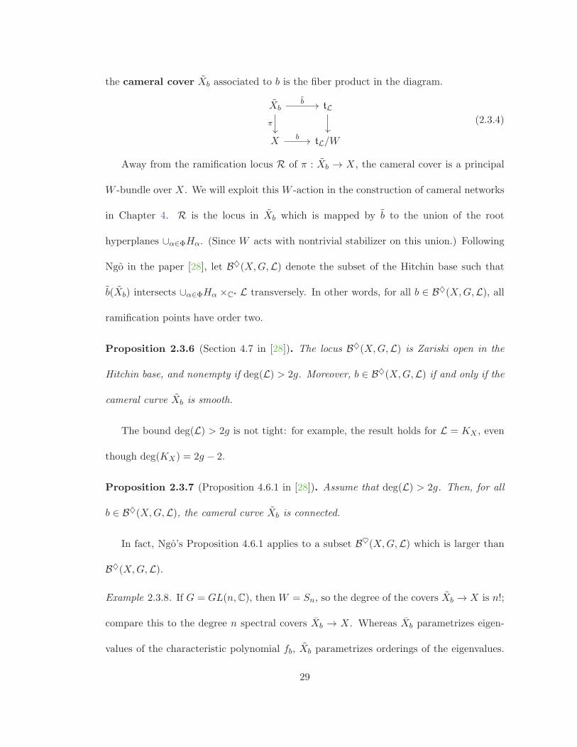
the cameral cover Xb associated to b is the fiber product in the diagram.

Xb tL

X tL/W

b

π

b

(2.3.4)

Away from the ramification locus R of π : Xb → X, the cameral cover is a principal

W -bundle over X. We will exploit this W -action in the construction of cameral networks

in Chapter 4. R is the locus in Xb which is mapped by b to the union of the root

hyperplanes ∪α∈ΦHα. (Since W acts with nontrivial stabilizer on this union.) Following

Ngo in the paper [28], let B♦(X,G,L) denote the subset of the Hitchin base such that

b(Xb) intersects ∪α∈ΦHα ×C∗ L transversely. In other words, for all b ∈ B♦(X,G,L), all

ramification points have order two.

Proposition 2.3.6 (Section 4.7 in [28]). The locus B♦(X,G,L) is Zariski open in the

Hitchin base, and nonempty if deg(L) > 2g. Moreover, b ∈ B♦(X,G,L) if and only if the

cameral curve Xb is smooth.

The bound deg(L) > 2g is not tight: for example, the result holds for L = KX , even

though deg(KX) = 2g − 2.

Proposition 2.3.7 (Proposition 4.6.1 in [28]). Assume that deg(L) > 2g. Then, for all

b ∈ B♦(X,G,L), the cameral curve Xb is connected.

In fact, Ngo’s Proposition 4.6.1 applies to a subset B♥(X,G,L) which is larger than

B♦(X,G,L).

Example 2.3.8. If G = GL(n,C), then W = Sn, so the degree of the covers Xb → X is n!;

compare this to the degree n spectral covers Xb → X. Whereas Xb parametrizes eigen-

values of the characteristic polynomial fb, Xb parametrizes orderings of the eigenvalues.

29

For generic enough b, and letting Sn−1 be the stabilizer of one of the eigenvalues, we have:

Xb/Sn−1∼= Xb. (2.3.5)

In particular, for n = 2, the spectral and cameral curves are isomorphic. More inter-

estingly, if n = 3 and two eigenvalues become equal at x ∈ X, then the local structure of

the spectral and cameral curves are as in Figure 2.1. There is extra symmetry present in

the cameral case.

Figure 2.1: Preimage of a branch point of order 2, in the spectral (left) and cameral

(right) curves.

The following theorem gives an analogue of the abelianization statement of Proposition

2.3.4.

Theorem 2.3.9 (Theorem 6.4 in [12]). The fiber of the Hitchin map over b ∈ B♦(X,G,L)

is isomorphic to the moduli space of weaklyW -equivariant, N -shifted, R-twisted T -bundles

on Xb.

We do not define here the meaning of the terms “weakly W -equivariant”, “N -shifted”

or “R-twisted”. The first two will be defined and used in Section 5.1; for the third, the

30

reader can consult [12]. For the purposes of this section, the take-away is that there exists

a moduli space of T -bundles on Xb, with appropriate extra data, which is isomorphic to

the Hitchin fiber over b.

31

Chapter 3

Lie theoretic technicalities

3.1 Chevalley bases and sl2-triples

This section is a collection of unoriginal results about the structure of reductive Lie

algebras. We present and organize the specific material from this subject area that will

be necessary in other sections.

Let g be a simple Lie algebra. We fix a Cartan subalgebra t, and let Φ denote the set

of roots of g. This determines a root space decomposition:

g = t⊕⊕α∈Φ

uα. (3.1.1)

Here the 1-dimensional root spaces uα are the α-eigenspaces for the adjoint action of the

Cartan.1 We will make frequent use of the following relationship between root spaces and

the Lie bracket.

1The root spaces are commonly denoted gα in the literature. We use uα instead, for compatibility with

the discussion of nilpotent Lie algebras and unipotent groups in Section 3.2.

32

Lemma 3.1.1. Let α, β ∈ Φ such that α �= −β. Then [uα, uβ ] ⊂ uα+β. Moreover,

[uα, uβ ] = 0 if and only if α+ β �∈ Φ.

Proof. Since the root spaces are 1-dimensional, so it suffices to consider the bracket [eα, eβ ]

for some choice of nonzero eα ∈ uα and eβ ∈ uβ . The Jacobi identity implies that, for all

h ∈ t:

[h, [eα, eβ ]

]=[[h, eα], eβ

]+[eα, [h, eβ ]

]=[α(h) · eα, eβ

]+[eα, β(h) · eβ

]= (α+ β)(h) · [eα, eβ ].

Hence [uα, uβ ] ⊂ uα+β .

It’s clear then that if α+β �∈ Φ, then [uα, uβ ] = 0. For the converse, see e.g. Theorem

6.44 in [26].

Definition 3.1.2. We say that a basis of g is adapted to the root space decompo-

sition if it consists of a basis for t, together with one nonzero element from each of the

root spaces uα.

In particular, there exist bases adapted to the root space decomposition, with respect

to which the structure constants are particularly well behaved.

Definition 3.1.3. Choose a polarization Φ = Φ+∐

Φ− of the root system; this deter-

mines a set ΦS ⊂ Φ+ of simple roots. A Chevalley basis is a basis of g compatible with

the root space decomposition, consisting of the data:

• {hα}α∈ΦS, which form a basis for t;

33

• {eγ}γ∈Φ;

such that the following conditions are satisfied. For all γ ∈ Φ, write γ =∑

α∈ΦSnαα, and

define hγ =∑

α∈ΦSnαhα. Then:

[hα, eγ ] = 2(α, γ)

(α, α)eγ , (3.1.2)

[eα, e−α] = −hα (3.1.3)

[eα, eγ ] =

⎧⎪⎪⎨⎪⎪⎩

0 if α+ γ �∈ Φ,

±(pα,γ + 1)eα+γ if α+ γ ∈ Φ.

(3.1.4)

In condition 3.1.4, pα,γ is defined as the largest integer such that α− pα,γγ ∈ Φ.

Remark 3.1.4. Conditions 3.1.2 and 3.1.3 imply that {hα, eα,−e−α} is an sl2-triple, for

every α ∈ Φ. We are using an uncommon sign convention in equation 3.1.3, which, in other

sources, is [eα, e−α] = hα. This would imply that {hα, eα, e−α} is an sl2-triple, which looks

like an aesthetically superior statement. However, we prefer our sign convention because

it allows us to treat eα and e−α on an equal footing down the line.

Remark 3.1.5. According to Lemma 3.1.1, if α+ γ ∈ Φ, then there must exist a constant

Cα,γ ∈ C∗ such that [eα, eγ ] = Cα,γ · eα+γ . Then it’s not hard to show that the constants

must satisfy Cα,γC−α,−γ = (pα,γ + 1)2. The choice made in equation 3.1.4 is Cα,γ =

C−α,−γ = ±(pα,γ + 1), which preserves the most symmetry between opposite roots. In

particular, the constants are small integers.

• For g of type ADE, the condition that α + γ ∈ Φ makes all pα,γ = 0. Therefore

Cα,γ = ±1.

• For g of type BCF, pα,γ = 1 if both roots are short, and 0 otherwise.

34

• For g of type G2, pα,γ ∈ {0, 1, 2}, depending on the angle between the roots.

To summarize Remarks 3.1.4 and 3.1.5, a Chevalley basis consists of sl2-triples whose

brackets are as simple as possible.

The following existence result was originally proved by Chevalley in [9], and a good

exposition is given by Tao in the blog post [37].

Proposition 3.1.6 (Chevalley, [9]). Every complex simple g admits a Chevalley basis.

Example 3.1.7. Let g = sl3, and α, β ∈ ΦS . We construct a Chevalley basis from the

following basis of the Cartan:

hα =

⎛⎜⎜⎜⎜⎜⎜⎝

1 0 0

0 −1 0

0 0 0

⎞⎟⎟⎟⎟⎟⎟⎠

hβ =

⎛⎜⎜⎜⎜⎜⎜⎝

0 0 0

0 1 0

0 0 −1

⎞⎟⎟⎟⎟⎟⎟⎠

(3.1.5)

and the following basis vectors for the root spaces:

eα =

⎛⎜⎜⎜⎜⎜⎜⎝

0 1 0

0 0 0

0 0 0

⎞⎟⎟⎟⎟⎟⎟⎠

eβ =

⎛⎜⎜⎜⎜⎜⎜⎝

0 0 0

0 0 1

0 0 0

⎞⎟⎟⎟⎟⎟⎟⎠

eα+β =

⎛⎜⎜⎜⎜⎜⎜⎝

0 0 1

0 0 0

0 0 0

⎞⎟⎟⎟⎟⎟⎟⎠

(3.1.6)

e−α =

⎛⎜⎜⎜⎜⎜⎜⎝

0 0 0

−1 0 0

0 0 0

⎞⎟⎟⎟⎟⎟⎟⎠

e−β =

⎛⎜⎜⎜⎜⎜⎜⎝

0 0 0

0 0 0

0 −1 0

⎞⎟⎟⎟⎟⎟⎟⎠

e−α−β =

⎛⎜⎜⎜⎜⎜⎜⎝

0 0 0

0 0 0

−1 0 0

⎞⎟⎟⎟⎟⎟⎟⎠

(3.1.7)

The set of Chevalley bases for sl3 is a torsor over the maximal torus TSL(3,C) ∼= (C∗)2.

For any re-scaling of eα, eβ by A,B ∈ C∗, it is possible to re-scale eα+β by AB, and

e−α, e−β , e−α−β by A−1, B−1, A−1B−1, respectively, so that relations 3.1.2 – 3.1.4 are

preserved.

35

Definition 3.1.8. Recall that a reductive Lie algebra g is the direct sum of its simple

sub-algebras and its abelian center. A Chevalley basis for g is the data of a Chevalley

basis for each simple summand, and an arbitrary basis for the center.

For the rest of the section, let g be complex reductive and fix a Chevalley basis for g.

Then each α ∈ Φ determines an sl2-triple, or equivalently a Lie algebra homomorphism

iα : sl2 → g. Because SL(2,C) is simply connected, Lie’s theorems (Theorem 3.41 in [26])

provide a group homomorphism Iα such that the following diagram commutes.

SL(2,C) G

sl2 g

Iα

exp

iα

exp (3.1.8)

Let sα ∈ W denote the reflection about the root hyperplane Hα, and denote by p

the quotient map N → T . The Chevalley basis determines, for each α ∈ Φ, an element

nα ∈ N ; Lemma 3.1.11 below proves that nα ∈ p−1(sα).

nα := exp[π2(eα + e−α)

]. (3.1.9)

Example 3.1.9. For g = sl2, and the Chevalley basis:

h =

⎛⎜⎜⎝ 1 0

0 −1

⎞⎟⎟⎠ e =

⎛⎜⎜⎝ 0 1

0 0

⎞⎟⎟⎠ − f =

⎛⎜⎜⎝ 0 0

−1 0

⎞⎟⎟⎠ , (3.1.10)

we have:

nSL(2,C) = exp[π2(e− f)

]=

⎛⎜⎜⎝ 0 1

−1 0

⎞⎟⎟⎠ . (3.1.11)

Due to diagram 3.1.8, nα = Iα(nSL(2,C)) is a characterization of nα.

Remark 3.1.10. Sending sα �→ nα does not, in general, give a section of the projection

p : N → W . Even in the case of SL(2,C), we have n2α = −id. For certain groups,

36

including SL(2,C), the normalizer short exact sequence below is not split.

1 T N W 1p

(3.1.12)

Lemma 3.1.11. nα is an element of the T -coset p−1(sα).

Proof. This follows from two observations:

1. adnα(hα) = −hα. This is proved by an easy computation in the case of sl2; then the

general case follows by applying iα. Note that Iα commutes with adjoint actions,

by virtue of being a homomorphism. Taking a differential, we obtain that iα also

does.

2. adnα(h) = h for h ∈ Hα. This is because of definition 3.1.9 and the fact that:

[h, e±α] = ±α(h)e±α = 0. (3.1.13)

The next result is a generalization of equation 1.1.10, and will similarly be used to

“cancel out” the monodromy of local systems around branch points.

Lemma 3.1.12. The following identity holds in G:

exp(eα) exp(e−α) exp(eα) = nα. (3.1.14)

Proof. Apply the homomorphism Iα to:⎛⎜⎜⎝ 1 1

0 1

⎞⎟⎟⎠⎛⎜⎜⎝ 1 0

−1 1

⎞⎟⎟⎠⎛⎜⎜⎝ 1 1

0 1

⎞⎟⎟⎠ =

⎛⎜⎜⎝ 0 1

−1 0

⎞⎟⎟⎠ . (3.1.15)

37

For every α ∈ Φ, the Killing form determines an orthogonal decomposition:

t = tα ⊕Hα, (3.1.16)

where tα is a 1-dimensional subspace generated by the co-root α∨, and Hα is the root

hyperplane satisfying α(Hα) = 0.

Let Tα = exp(tα) and THα = exp(Hα). Tα is characterized as Iα(TSL(2)).

Lemma 3.1.13. The multiplication homomorphism:

Tα × THα −→ T (3.1.17)

is surjective. Its kernel is trivial if Iα factors through PSL(2,C), otherwise it is:

{(id, id),

(Iα(−idSL(2)), Iα(−idSL(2))

)}. (3.1.18)

Proof. Due to the orthogonal decomposition 3.1.16 at the Lie algebra level, multiplication

Tα × THα → T is surjective. Its finite kernel is the intersection Tα ∩ THα in T . Since

Tα = Iα(TSL(2,C)), and THα is in the kernel of the character exp(α), we need only analyze

the diagram:

TSL(2) T C×.Iα exp(α)(3.1.19)

It follows that:

Tα ∩ THα = Iα(Ker(exp(α) ◦ Iα)

). (3.1.20)

Denote exp(αSL(2)) = exp(α) ◦ Iα; so it suffices to show that Ker(exp(αSL(2))) =

{±idSL(2)}. Ker(exp(αSL(2))) consists of the elements of TSL(2) whose adjoint action fixes

eαSL(2); the latter is either: ⎛

⎜⎜⎝ 0 1

0 0

⎞⎟⎟⎠ or

⎛⎜⎜⎝ 0 0

−1 0

⎞⎟⎟⎠ .

38

Either way, {±idSL(2)} are the only elements of TSL2 whose adjoint action fixes it.

Lemma 3.1.14. The adjoint action of nα satisfies:

1. For every t ∈ Tα, nαtn−1α = t−1.

2. For every t ∈ THα, nαtn−1α = t.

Proof. An immediate consequence of Lemma 3.1.11.

We state two more results which are necessary in section 5.3.1. Their elementary

proofs can be found in [23].

Lemma 3.1.15. For all t ∈ T , adt(eα) is a scalar multiple of eα. Moreover, all scalar

multiples of eα arise in this way.

Lemma 3.1.16. Let n ∈ N , and [n] ∈W its image in the Weyl group. Define α′ = [n](α).

Then there exists some t ∈ Tα′ such that:

• adn(e±α) = adt(e±α′);

• Adn(nα) = Adt(nα′).

3.2 Scattering diagrams and Stokes factors

In this section we introduce 2D scattering diagrams (Definition 3.2.11), which are a local

model for the intersections of Stokes curves that will appear in Chapters 4 and 5. Each

ray in the scattering diagram is labeled by a root α of g, and decorated by an element

of exp(uα) called a Stokes factor. The main goal of the section is to prove, in as much

39

generality as possible, that the Stokes factors for incoming rays uniquely determine the

Stokes factors for outgoing rays (Theorem 3.2.21).

We first make some definitions related to sets of roots.

Definition 3.2.1. We say that a set of roots C ⊂ Φ is convex if there exists a polarization

Φ = Φ+∐

Φ− such that C ⊂ Φ+.

Equivalently, C is convex if it is contained in a strictly convex cone in t∗ with vertex

at the origin.

Definition 3.2.2. Let {α1, . . . , αj} be a convex set of roots. Their restricted convex

hull is the subset:

ConvNα1,...,αj:=

{γ ∈ Φ

∣∣∣∣γ =

j∑i=1

niαi, ni ∈ N

}. (3.2.1)

For comparison, their convex hull is:

Convα1,...,αj :=

{γ ∈ Φ

∣∣∣∣γ =

j∑i=1

niαi, ni ∈ R+

}. (3.2.2)

In this paper we will mostly need the restricted convex hull.

The restricted convex hull is motivated by the following reformulation of Lemma 3.1.1.

Lemma 3.2.3. Let α, β ∈ Φ, such that α �= ±β. Then the Lie subalgebra of g generated

by uα and uβ is spanned, as a vector space, by uγ with γ ranging over ConvNα,β.

Proof. Due to Lemma 3.1.1, [uα, uβ ] = uα+β if α + β ∈ Φ, and [uα, uβ ] = 0 otherwise.

By recursive application of this result, we obtain that 〈uα, uβ〉 contains uγ if and only if

γ ∈ ConvNα,β .

40

Example 3.2.4. In root systems of type ADE, for every convex pair of roots {α1, α2},

Convα1,α2 = ConvNα1,α2. To see this, note that the restriction of the root system to the

plane spanned by α1 and α2 is a root system of type A1 × A1 or A2. In both cases, the

claim is obvious. (See Figures 3.1 and 3.2.)

Figure 3.1: The root system A1 ×A1Figure 3.2: The root system A2

Example 3.2.5. In a root system of type B2 (see Figure 3.3), let α1, α2 be orthogonal long

roots. Then:

Convα1,α2 = {α1, (α1 + α2)/2, α2},

ConvNα1,α2= {α1, α2}.

In Section 3.3 we give other explicit examples and computations, in the case of the

planar root systems of Figures 3.1–3.4. In the meantime, we comment on the difference

between ConvC and ConvNC for non-planar root systems.

Lemma 3.2.6. For g a simple Lie algebra of type A, and C ⊂ Φ+, ConvC = ConvNC .

Proof. Let Π = {α1, . . . , αn} be the set of simple roots determined by the polarization

Φ+, and recall that Π is a basis for the root system; in particular, for any γ ∈ Φ+, there

41

Figure 3.3: The root system B2

Figure 3.4: The root system G2

is a unique expression:

γ =

n∑k=1

akαk, ak ∈ N. (3.2.3)

We need some facts about positive roots:

1. For any simple g, the support of γ ∈ Φ+, defined as those αk for which the coefficient

ak in equation 3.2.3 is nonzero, is a connected subset of the Dynkin diagram. (See

corollary 3 to Proposition VI.1.6.19 of [6].)

2. For g of type A, all nonzero coefficients in 3.2.3 are equal to 1. To see this, we

assume without loss of generality that Φ+ corresponds to upper-triangular matrices

in sln, so that the simple roots correspond to the entries immediately above the

diagonal: ⎛⎜⎜⎜⎜⎜⎜⎜⎜⎜⎜⎝

α1

. . .

αn

⎞⎟⎟⎟⎟⎟⎟⎟⎟⎟⎟⎠. (3.2.4)

42

Then the positive root γij , corresponding to the root space of the elementary matrix

Eij , for i < j, satisfies γij =∑j−1

k=i αk.

By the above facts, in the case of g of type A, sending a positive root to its support gives

a bijection between Φ+ and discrete intervals {i, j} ⊂ {1, n}, where we define:

{i, j} := [i, j] ∩ Z. (3.2.5)

Moreover, this bijection maps the sum of roots to the union of discrete intervals.

Assume, then, that C = {γ1, . . . , γd} ⊂ Φ+, and γ0 ∈ ConvC , i.e.:

γ0 =

d∑i=1

ciγi, ci ∈ [0,∞). (3.2.6)

For every i, let Ii ⊂ {1, n} denote the support of γi; then Ii ⊂ I0, for every i > 0. We

assume without loss of generality that I0 = {1, n}, otherwise we could restrict to the

sub-root system generated by the support of γ0.

We claim that there exist {ij}lj=1 such that I0 =∐l

j=1 Iij , from which it follows that

γ0 =∑l

j=1 γij , so in particular γ0 ∈ ConvNC . We prove this claim as follows.

• Choose i1 be such that 1 ∈ Ii1 and ci1 �= 0. Such an index must exist, otherwise the

simple root α1 wouldn’t be in the support of γ0.

• Let end1 denote the endpoint of Ii1 . Choose i2 such that Ii2 starts at end1 + 1,

and ci2 �= 0. Such an index must exist, otherwise the coefficient of α1 in the basis

expansion of γ0 would be greater than the coefficient of α2, contradicting the fact

that both coefficients are equal to 1.

• Continue this process, terminating at step l, when the discrete interval Iil ends at

43

n. This must happen eventually, otherwise the simple root αn wouldn’t be in the

support of γ0.

It might be tempting, based on Lemma 3.2.6 and the previous examples, to conjecture

that ConvC = ConvNC for Lie algebras of type ADE. However, this is false as soon as we

leave type A, as the following example shows.

Example 3.2.7. Consider the reduced root system of type D4, whose Dynkin diagram is

shown in figure 3.5.

Figure 3.5: Dynkin diagram for D4, with simple roots labeled.

Beyond type A, fact 1 from the proof of Lemma 3.2.6 is still true, but fact 2 is not,

i.e. supports of positive roots are still connected subsets of the Dynkin diagram, but the

coefficients can be greater than 1. Consider the positive roots:

γ0 = α+ β + γ + δ,

γ1 = α,

γ2 = γ,

γ3 = δ,

γ4 = α+ 2β + γ + δ,

(3.2.7)

44

and let C = {γ1, γ2, γ3, γ4}. Then:

γ0 =1

2(γ1 + γ2 + γ3 + γ4), (3.2.8)

which shows that γ0 ∈ ConvC , but γ0 �∈ ConvNC .

Before we define 2D scattering diagrams, we associate unipotent groups to certain

convex subsets of Φ.

Lemma 3.2.8. Let C ⊂ Φ be a convex subset, closed under addition. (Equivalently,

C = ConvNC .) Consider the Lie sub-algebra of g, spanned as a vector space by:

uC :=⊕γ∈C

uγ . (3.2.9)

Then uC is nilpotent.

Proof. Due to the convexity assumption, there exists a polarization Φ = Φ+∐

Φ− of the

root system, such that C ⊂ Φ+. Recall that the Lie algebra:

n+ =⊕α∈Φ+

gα (3.2.10)

is nilpotent. Since uC ⊂ n+, and Lie subalgebras of nilpotent Lie algebras are nilpotent,

the claim follows.

Definition 3.2.9. For any C ⊂ Φ+ closed under addition, let UC := exp(uC) be the

associated unipotent subgroup of G.

Remark 3.2.10. For any nilpotent Lie algebra u, the exponential map exp : u → U is

algebraic, because the Taylor series of the exponential is finite in this case. Therefore, all

constructions in this section that involve the exponential map makes sense in the setting

of algebraic groups. Moreover, for u nilpotent, exp : u → U is an isomorphism of schemes.

45

Definition 3.2.11. Let Cin ⊂ Φ be a convex set, and set Cout = ConvNCin. An undeco-

rated 2D scattering diagram is a finite collection of oriented rays in R2, starting or

ending at {0} ∈ R2, together with the data of:

• a bijection between the set of incoming rays and Cin (we say that incoming rays are

labeled by elements of Cin);

• a bijection between the set of outgoing rays and Cout.

A decorated 2D scattering diagram is an undecorated 2d scattering diagram together

with:

• For every ray with label α, an element uα ∈ Uα called the Stokes factor.

The Stokes factors are required to satisfy a constraint. The product taken over both

incoming and outgoing Stokes factors, in clockwise order around the intersection point,

is the identity:

−→∏α∈Cin

∐Cout

u±1α = id. (3.2.11)

Here−→∏

denotes the clockwise-ordered product, and the exponent accounts for orientation:

it is −1 for incoming rays, and +1 for outgoing rays.

Definition 3.2.12. A solution to an (undecorated) 2D scattering diagram is a

way to assign Stokes factors uγ ∈ Uγ to the outgoing half-lines, given arbitrary Stokes

factors on the incoming rays, such that the result is a decorated 2D scattering diagram.

Concretely, it is a morphism of schemes:

∏α∈Cin

Uα →∏

γ∈Cout

Uγ , (3.2.12)

46

such that the product in 3.2.11, taken over the inputs and outputs of the morphism, is

the identity.

Example 3.2.13. Let g = sl3, and α, β be a choice of simple roots such that the root spaces

are: ⎛⎜⎜⎜⎜⎜⎜⎝

uα uα+β

u−α uβ

u−α−β u−β

⎞⎟⎟⎟⎟⎟⎟⎠. (3.2.13)

Figure 3.6 depicts an undecorated 2D scattering diagram, with incoming rays labeled by

α, β and outgoing rays labeled by α, α+ β, β.

Figure 3.6: A 2D scattering diagram.

A solution for this 2D scattering diagram is a morphism:

Uα × Uβ −→ Uβ × Uα+β × Uα

(uα, uβ) �−→ (u′β , u′α+β , u

′α),

(3.2.14)

such that:

u′αu′α+βu

′βu

−1α u−1

β = id. (3.2.15)

Equivalently, we need to produce u′α, u′β , u′α+β such that u′αu′α+βu

′β = uβuα. With the

Chevalley basis for sl3 from Example 3.1.7, let uα = exp(xeα), uβ = exp(yeβ), u′α =

47

exp(x′eα), u′β = exp(y′eβ), u′α+β = exp(z′eα+β). Then:

uβuα =

⎛⎜⎜⎜⎜⎜⎜⎝

1 0 0

0 1 y

0 0 1

⎞⎟⎟⎟⎟⎟⎟⎠

⎛⎜⎜⎜⎜⎜⎜⎝

1 x 0

0 1 0

0 0 1

⎞⎟⎟⎟⎟⎟⎟⎠

=

⎛⎜⎜⎜⎜⎜⎜⎝

1 x 0

0 1 y

0 0 1

⎞⎟⎟⎟⎟⎟⎟⎠, (3.2.16)

u′αu′α+βu

′β =

⎛⎜⎜⎜⎜⎜⎜⎝

1 x′ 0

0 1 0

0 0 1

⎞⎟⎟⎟⎟⎟⎟⎠

⎛⎜⎜⎜⎜⎜⎜⎝

1 0 z′

0 1 0

0 0 1

⎞⎟⎟⎟⎟⎟⎟⎠

⎛⎜⎜⎜⎜⎜⎜⎝

1 0 0

0 1 y′

0 0 1

⎞⎟⎟⎟⎟⎟⎟⎠

=

⎛⎜⎜⎜⎜⎜⎜⎝

1 x′ z′ + x′y′

0 1 y′

0 0 1

⎞⎟⎟⎟⎟⎟⎟⎠,

(3.2.17)

whence we read off x′ = x, y′ = y, z′ = −xy. In other words, the unique solution is:

u′α = uα, (3.2.18)

u′β = uβ , (3.2.19)

u′α+β = u−1α uβuαu

−1β . (3.2.20)

In the rest of this section, we work towards a proof of existence and uniqueness of

solutions to 2D scattering diagrams, which does not rely on explicit computations such

as the ones in Example 3.2.13. The final result is Theorem 3.2.21.

Proposition 3.2.14. Let C ⊂ Φ be a convex subset such that C = ConvNC . Then multi-

plication gives an isomorphism of schemes:

∏γ∈C

UγM−→ UC , (3.2.21)

for any ordering of the product on the left hand side.

Proof. We use the Baker-Campbell-Hausdorff formula:

exp(X) exp(Y ) = exp

(X + Y +

1

2[X,Y ] + . . .

), (3.2.22)

48

where the dots indicate higher order iterated Lie brackets of X and Y . We only need this

formula for the case when each of X, Y spans a root space of g. Due to Lemma 3.1.1 and

the convexity assumption, there are only finitely many nonzero iterated Lie brackets in

this case.

For all γ ∈ C, let Xγ ∈ uγ . Applying the Baker-Campbell-Hausdorff formula itera-

tively, we obtain:

∏γ∈C

exp(Xγ) = exp

⎛⎝∑

γ∈C(Xγ + junkγ)

⎞⎠ , (3.2.23)

where junkγ is the sum of all iterated Lie brackets which belong to the root space uγ .

It follows that we have a commutative diagram of schemes:∏γ∈C Uγ UC

⊕γ∈C uγ uC ,

M

∏γ∈C exp

m

exp (3.2.24)

where m is the map:

(Xγ)γ∈C �−→∑γ∈C

Xγ + junkγ . (3.2.25)

The vertical arrows are isomorphisms of schemes (because the Lie groups are unipotent),

so it suffices to prove thatm is invertible. Because we can composem with the projections

uC → uγ , invertibility means recovering the input tuple (Xγ)γ∈C from the output tuple

(Xγ + junkγ)γ∈C . We will argue by induction on the height of γ ∈ C, so let us recall the

concept of height of a root.

Since C is convex, there exists a polarization Φ = Φ+∐

Φ− such that C ⊂ Φ+. Let

{α1, . . . , αd} denote the simple roots with respect to this polarization, and recall that the

simple roots are a basis for the root system. Then all γ ∈ C can be written uniquely as:

γ =

d∑i=1

niαi, ni ∈ N. (3.2.26)

49

Then we define the height of γ as ht(γ) =∑d

i=1 ni. In particular, ht(γ1) + ht(γ2) =

ht(γ1 + γ2).

Using Lemma 3.1.1, we obtain that, if [Xβ , Xδ] ∈ uγ , then ht(β), ht(δ) < ht(γ).

Generalizing, if an iterated Lie bracket involving Xβ belongs to uγ , then ht(β) < ht(γ).

In other words, junkγ only depends on those Xβ with ht(β) < ht(γ).

The inductive argument is as follows. The base case is given by all γ of minimal height:

for these, junkγ = 0, and the composition of m with the projection uC → uγ recovers Xγ .

For the inductive step, assume we know Xβ for all β ∈ C such that ht(β) < ht(γ). These

determine junkγ , so we can recover Xγ uniquely from the output of 3.2.25.

Example 3.2.15. For g = sl3, choose a polarization so that the positive root spaces corre-

spond to upper-triangular matrices. We have the explicit formula:⎛⎜⎜⎜⎜⎜⎜⎝

1 a 0

0 1 0

0 0 1

⎞⎟⎟⎟⎟⎟⎟⎠

⎛⎜⎜⎜⎜⎜⎜⎝

1 0 c

0 1 0

0 0 1

⎞⎟⎟⎟⎟⎟⎟⎠

⎛⎜⎜⎜⎜⎜⎜⎝

1 0 0

0 1 b

0 0 1

⎞⎟⎟⎟⎟⎟⎟⎠

=

⎛⎜⎜⎜⎜⎜⎜⎝

1 a c+ ab

0 1 b

0 0 1

⎞⎟⎟⎟⎟⎟⎟⎠

= exp

⎛⎜⎜⎜⎜⎜⎜⎝

0 a c+ ab/2

0 0 b

0 0 0

⎞⎟⎟⎟⎟⎟⎟⎠

The map (a, b, c) �→ (a, b, c+ ab/2) is clearly invertible.

Proposition 3.2.14 is really a statement about root spaces. If we use a basis for g that

is not adapted to the root space decomposition, then the result need not be true.

Example 3.2.16. Let g = sl3, and choose the following basis for the Lie subalgebra of

50

strictly upper triangular matrices:⎛⎜⎜⎜⎜⎜⎜⎝

0 1 1

0 0 0

0 0 0

⎞⎟⎟⎟⎟⎟⎟⎠,

⎛⎜⎜⎜⎜⎜⎜⎝

0 0 0

0 0 1

0 0 0

⎞⎟⎟⎟⎟⎟⎟⎠,

⎛⎜⎜⎜⎜⎜⎜⎝

0 1 −1

0 0 0

0 0 0

⎞⎟⎟⎟⎟⎟⎟⎠. (3.2.27)

Then: ⎛⎜⎜⎜⎜⎜⎜⎝

1 a a

0 1 0

0 0 1

⎞⎟⎟⎟⎟⎟⎟⎠

⎛⎜⎜⎜⎜⎜⎜⎝

1 0 0

0 1 b

0 0 1

⎞⎟⎟⎟⎟⎟⎟⎠

⎛⎜⎜⎜⎜⎜⎜⎝

1 c −c

0 1 0

0 0 1

⎞⎟⎟⎟⎟⎟⎟⎠

=

⎛⎜⎜⎜⎜⎜⎜⎝

1 a+ c a− c+ ab

0 1 b

0 0 1

⎞⎟⎟⎟⎟⎟⎟⎠.

Elements of the form: ⎛⎜⎜⎜⎜⎜⎜⎝

1 x z

0 1 y

0 0 1

⎞⎟⎟⎟⎟⎟⎟⎠

(3.2.28)

with y = −2 and x �= −z form a codimension 1 locus not in the image of the multiplication

map.

Corollary 3.2.17. Consider a 2D scattering diagram where incoming rays are constrained

to a sector of the plane with central angle < π, and the outgoing rays are constrained to

the opposite sector. The situation is depicted in Figure 3.7. Then the scattering diagram

has a unique solution.

Proof. Due to the assumption about separation of incoming and outgoing rays, equation

3.2.11 has the form:

−→∏α∈Cinu

−1α

−→∏γ∈Coutuγ = id. (3.2.29)

All factors in the first product are known, and all factors in the second product must be

51

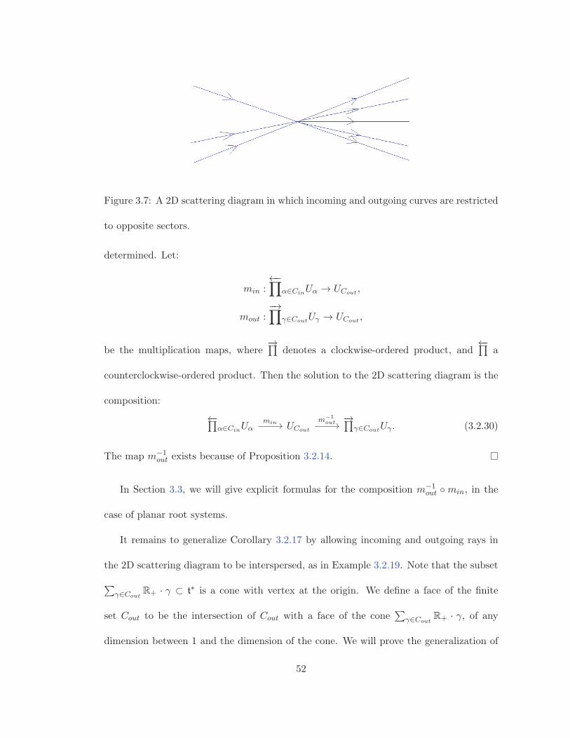
Figure 3.7: A 2D scattering diagram in which incoming and outgoing curves are restricted

to opposite sectors.

determined. Let:

min :←−∏

α∈CinUα → UCout ,

mout :−→∏

γ∈CoutUγ → UCout ,

be the multiplication maps, where−→∏

denotes a clockwise-ordered product, and←−∏

a

counterclockwise-ordered product. Then the solution to the 2D scattering diagram is the

composition:

←−∏α∈CinUα UCout

−→∏γ∈CoutUγ .

min m−1out (3.2.30)

The map m−1out exists because of Proposition 3.2.14.

In Section 3.3, we will give explicit formulas for the composition m−1out ◦min, in the

case of planar root systems.

It remains to generalize Corollary 3.2.17 by allowing incoming and outgoing rays in

the 2D scattering diagram to be interspersed, as in Example 3.2.19. Note that the subset

∑γ∈Cout

R+ · γ ⊂ t∗ is a cone with vertex at the origin. We define a face of the finite

set Cout to be the intersection of Cout with a face of the cone∑

γ∈CoutR+ · γ, of any

dimension between 1 and the dimension of the cone. We will prove the generalization of

52

Corollary 3.2.17 by induction on the dimension of the faces of Cout. Throughout, we use

the notation Δ ⊂ Cout to denote a face of Cout.

Lemma 3.2.18. Let Δf ⊂ Δ be a face. The projection pf : uΔ → uΔfwith kernel

⊕γ∈CΔ\CΔfuγ is a morphism of Lie algebras.

Consequently, there is a group homomorphism UΔ → UΔf, which acts as the identity

on UΔfand sends every element of the form exp(Xγ) (Xγ ∈ uγ), for γ �∈ Δf , to idUΔf

.

Proof. We need to prove that pf([X1, X2]

)=[pf (X1), pf (X2)

], for all X1, X2 ∈ uΔ. We

analyze two cases.

• If X1, X2 ∈ uΔf, then [X1, X2] ∈ uΔf

, due to Lemma 3.1.1. So pf leaves each of

X1, X2, [X1, X2] unchanged.

• If at least one of X1, X2 is not in uΔf, then, using Lemma 3.1.1 and the assumption

that Δf is a face, either [X1, X2] = 0 or [X1, X2] �∈ uΔf. The equality pf

([X1, X2]

)=

[pf (X1), pf (X2)

]holds with both sides equal to 0.

The following easy example demonstrates our strategy for assigning Stokes factors to

outgoing rays in 2D scattering diagrams, making use of Lemma 3.2.18. We then generalize

and formalize this strategy in Theorem 3.2.21.

Example 3.2.19. Let g = sl4, and consider the polarization such that the positive roots

correspond to strictly upper triangular matrices. Let α, β, γ denote the simple roots.

53

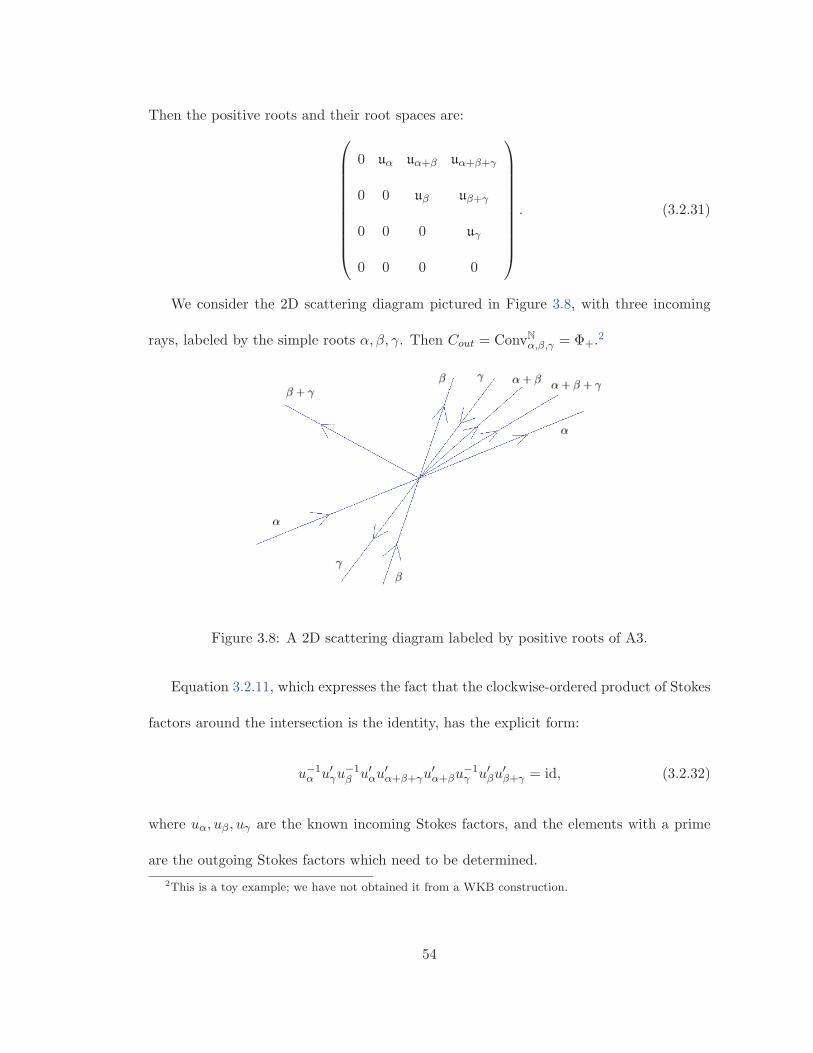
Then the positive roots and their root spaces are:⎛⎜⎜⎜⎜⎜⎜⎜⎜⎜⎜⎝

0 uα uα+β uα+β+γ

0 0 uβ uβ+γ

0 0 0 uγ

0 0 0 0

⎞⎟⎟⎟⎟⎟⎟⎟⎟⎟⎟⎠. (3.2.31)

We consider the 2D scattering diagram pictured in Figure 3.8, with three incoming

rays, labeled by the simple roots α, β, γ. Then Cout = ConvNα,β,γ = Φ+.2

Figure 3.8: A 2D scattering diagram labeled by positive roots of A3.

Equation 3.2.11, which expresses the fact that the clockwise-ordered product of Stokes

factors around the intersection is the identity, has the explicit form:

u−1α u′γu

−1β u′αu

′α+β+γu

′α+βu

−1γ u′βu

′β+γ = id, (3.2.32)

where uα, uβ , uγ are the known incoming Stokes factors, and the elements with a prime

are the outgoing Stokes factors which need to be determined.

2This is a toy example; we have not obtained it from a WKB construction.

54

Figure 3.9: A cross-section of the cone Φ+ in the root system A3.

Figure 3.9 shows a cross-section of the cone structure on Cout, with labels indicating 1-

dimensional faces. Let Δ denote the 2D face spanned by α and β. The image of equation

3.2.32 under the projection UCout → UΔ is:

u−1α u−1

β u′αu′α+βu

′β = id. (3.2.33)

Projecting further to the 1-dimensional face spanned by α, we obtain uα = u′α. Anal-

ogously, we obtain uβ = u′β . Plugging these back into 3.2.33 gives:

u′α+β = u−1α uβuαu

−1β . (3.2.34)

As a sanity check, we would like to have u′α+β ∈ Uα+β . The RHS of equation 3.2.34 is

in the kernel of both projections UΔ → Uα and UΔ → Uβ . The intersection of the two

kernels is precisely Uα+β .

The elements u′γ , u′β+γ are determined analogously. Then u′α+β+γ is the only remaining

unknown in 3.2.32, so it is uniquely determined:

u′α+β+γ = u−1α uβu

−1γ uα(u

−1β uγuβu

−1γ )u−1

β uγ(uβu−1α u−1

β uα). (3.2.35)

Again, this element is in the intersection of the kernels of all face projections, which is

55

Uα+β+γ .

Example 3.2.19 was made easy by the fact that, at every stage, there is at most a single

root which doesn’t lie on one of the faces. Clearly, we cannot expect this simplification in

general: figures 3.3, 3.4 show that this fails for the root systems B2 and G2, respectively.

In fact, it even fails for simply laced root systems beyond type A, as the following example

shows.

Example 3.2.20. Consider the root system D4, with simple roots {α, β, γ, δ} as labeled on

the Dynkin diagram in Figure 3.5. The positive roots, ordered by the dimension of the

smallest-dimensional face they lie on, are:

1 : α, β, δ, γ,

2 : α+ β, β + γ, β + δ,

3 : α+ β + γ, α+ β + δ, β + γ + δ,

4 : α+ β + γ + δ, α+ 2β + γ + δ.

There are two roots in the interior of the 4-dimensional cone.

The following result generalizes the strategy of Example 3.2.19 appropriately. For

convenience, we introduce some notation for an ordered product of unipotent elements.

Let Δ be a face of Cout of arbitrary dimension. Then we define:

uΔ :=−→∏

γ∈(Cin∩Δ)∐

(Cout∩Δ)(uγ)±1 (3.2.36)

as a product over all Stokes factors corresponding to roots γ ∈ Δ, taken in clockwise

order around the intersection, where the exponent is +1 for outgoing curves, and −1 for

56

incoming curves. Note that equation 3.2.11, expressing the constraint that a solution to

a 2D scattering diagram must satisfy, can be rewritten as uCout = id.

Theorem 3.2.21. Every 2D scattering diagram has a unique solution. Concretely, this

means that there is a unique morphism of schemes:

∏γ∈Cin

Uγ −→∏

γ∈Cout

Uγ

(uγ)γ∈Cin �−→ (u′γ)γ∈Cout

such that uCout = id, using the notation of equation 3.2.36. Moreover, for every input

tuple (uγ)γ∈Cin, (u′γ)γ∈Cout is the unique output tuple such that uCout = id.

Proof. The proof is by induction on the dimension of the faces Δ of Cout, and can be

found in [23].

3.3 Explicit calculations for planar root systems

In this section we list a few explicit calculations, which exemplify the results of Section

3.2 in the case of planar root systems. Recall that there are only four planar root systems;

they are depicted in Figures 3.1-3.4.

Lemma 3.3.1. Choose a polarization of the planar root system, and let α, β be the simple

roots determined by the polarization. If their lengths differ, let α be the shorter root.

Then the restricted convex hull (see Definition 3.2.2) coincides with the convex hull, and

is explicitly given by:

1. Convα,β = {α, β} in the A1 ×A1 case;

57

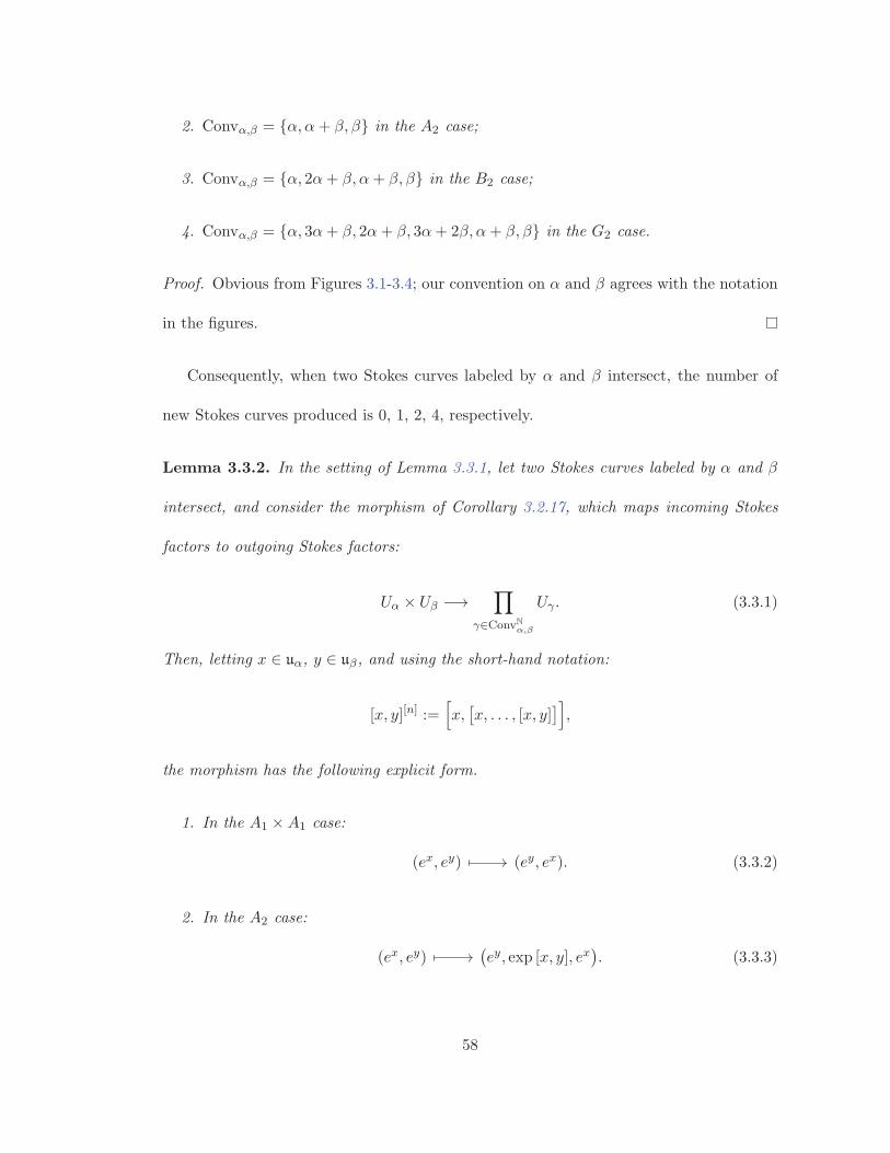
2. Convα,β = {α, α+ β, β} in the A2 case;

3. Convα,β = {α, 2α+ β, α+ β, β} in the B2 case;

4. Convα,β = {α, 3α+ β, 2α+ β, 3α+ 2β, α+ β, β} in the G2 case.

Proof. Obvious from Figures 3.1-3.4; our convention on α and β agrees with the notation

in the figures.

Consequently, when two Stokes curves labeled by α and β intersect, the number of

new Stokes curves produced is 0, 1, 2, 4, respectively.

Lemma 3.3.2. In the setting of Lemma 3.3.1, let two Stokes curves labeled by α and β

intersect, and consider the morphism of Corollary 3.2.17, which maps incoming Stokes

factors to outgoing Stokes factors:

Uα × Uβ −→∏

γ∈ConvNα,β

Uγ . (3.3.1)

Then, letting x ∈ uα, y ∈ uβ, and using the short-hand notation:

[x, y][n] :=[x,[x, . . . , [x, y]

]],

the morphism has the following explicit form.

1. In the A1 ×A1 case:

(ex, ey) (ey, ex). (3.3.2)

2. In the A2 case:

(ex, ey)(ey, exp [x, y], ex

). (3.3.3)

58

3. In the B2 case:

(ex, ey)

(ey, exp [x, y], exp

(12 [x, y]

[2]), ex). (3.3.4)

4. In the G2 case:

(ex, ey)

(ey, exp [x, y], exp

(16

[[x, y][2], [x, y]

]), exp

(12 [x, y]

[2]), exp

(16 [x, y]

[3]), ex

).

(3.3.5)

Proof. Using Lemma 3.1.1, and the explicit description of ConvNα,β from Lemma 3.3.1,

it’s clear that the given elements live in the correct one-parameter subgroups Uγ , for

γ ∈ ConvNα,β . It suffices, then, to prove that:

exey = ey exp [x, y] exp

(1

6

[[x, y][2], [x, y]

])exp

(1

2[x, y][2]

)exp

(1

6[x, y][3]

)ex, (3.3.6)

where we allow the possibility that some of the exponents are zero, in order to treat all

four cases simultaneously.

Up to order 5 in x, y ∈ g, the Baker-Campbell-Hausdorff formula gives:

log(exey) = x+ y +1

2[x, y] +

1

12

([x, [x, y]

]+[y, [y, x]

])− 1

24

[x,[y, [x, y]

]]−− 1

720

([y,[y,[y, [y, x]

]]]+

[x,[x,[x, [x, y]

]]])+

+1

360

([y,[x,[x, [x, y]

]]]+

[x,[y,[y, [y, x]

]]])+

+1

720

([y,[x,[y, [x, y]

]]]+

[x,[y,[x, [y, x]

]]])+

+ . . .

(3.3.7)

See, for example, Theorem 2 in II.6.6 of [6] for the general combinatorial formula, originally

due to Dynkin.

59

Now let x ∈ uα, y ∈ uβ . Lemma 3.3.1 ensures that the only nonzero terms are:

log(exey) = x+ y +1

2[x, y] +

1

12[x, y][2] +

1

360

[[x, y][2], [x, y]

]. (3.3.8)

Similarly:

log

(ey exp [x, y] exp

(1

6

[[x, y][2], [x, y]

]))=y + [x, y] +

1

6

[[x, y][2], [x, y]

], (3.3.9)

log

(exp

(1

2[x, y][2]

)exp

(1

6[x, y][3]

)ex)

=1

2[x, y][2] +

1

6[x, y][3] + x+

+1

4

[[x, y][2], x

]=x+

1

2[x, y][2] − 1

12[x, y][3].

(3.3.10)

Let z, w denote the right-hand sides of 3.3.9 and 3.3.10, respectively. Then we need

to prove that exey = ezew. The nonzero iterated Lie brackets of z, w are:

[z, w] = −[x, y]− [x, y][2] − 7

12

[[x, y][2], [x, y]

],

[z, w][2] =[[x, y][2], [x, y]

],

[w, z][2] = [x, y][2] + [x, y][3] +1

2

[[x, y][2], [x, y]

],

[[w, z][2], [w, z]

]=[[x, y][2], [x, y]

].

Then:

log(ezew) = z + w +1

2[z, w] +

1

12[z, w][2] +

1

12[w, z][2] +

1

360

[[w, z][2], [w, z]

]= x+ y +

1

2[x, y] +

1

12[x, y][2] +

1

360

[[x, y][2], [x, y]

].

This agrees with log(exey), as computed in 3.3.8.

Consider an intersection of k curves, labeled by a maximal planar, convex, set of roots,

as in Figure 3.10.

60

Figure 3.10: Intersection corresponding to maximal planar, convex set of roots.

Let γ1, . . . , γk denote the order on ConvNα,β induced by the order of the incoming Stokes

curves. Then the outgoing curves have the reverse order. So, in this case, Corollary 3.2.17

gives a morphism which commutes with the multiplication maps:

Uγ1 × · · · × Uγk UConvNα,β

Uγk × · · · × Uγ1

reverse (3.3.11)

We now explain how to obtain explicit formulas for the morphism reverse, by repeated

application of Lemma 3.3.2.

We use the fact that, in the planar case we are dealing with, the order on outgoing

Stokes curves is convex. This means that, if there are three outgoing curves labeled by

γ, δ, γ + δ, then the one labeled by γ + δ lies within the sector bounded by the curves

labeled by γ and δ. (See Lemma 4.1.17.) There are only two total orders on ConvNα,β

satisfying this convexity property: they are {γ1, . . . , γk} and its reverse {γk, . . . , γ1}, both

considered in diagram 3.3.11. Since the order on ConvNα,β used on the RHS of Lemma

3.3.2 is convex, it must coincide with one of these two. We assume that it is {γk, . . . , γ1};

otherwise, we would describe reverse−1 instead.

We build the morphism reverse as a composition of “twisted transpositions” and “con-

61

tractions”, as defined below.

We define a twisted transposition to be an application of Lemma 3.3.2: we replace

an element of a product of two neighboring factors, Uγi × Uγj such that i < j, with the

tuple provided by the RHS of Lemma 3.3.2. The requirement that i < j ensures that the

resulting tuple is ordered correctly.

We define a contraction to be a multiplication map:

Uγi × Uγi → Uγi . (3.3.12)

It is clear that, using finitely many twisted transpositions and contractions, we obtain

a morphism which commutes with the multiplication maps as in diagram 3.3.11. This

must agree with reverse, due to the uniqueness statement in Corollary 3.2.17.

Example 3.3.3 (Cecotti–Vafa Wall Crossing Formula). Consider a Lie algebra g of ADE

type. The restriction of the root system to the plane spanned by α and β is a root system

of type A1×A1 or A2. In the first case, k = 2, and we have reverse(eXα , eXβ ) = (eXβ , eXα),

an honest transposition. In the second case, k = 3 and the commutativity of the diagram

3.3.11 is expressed by:

exp(Xα) exp(Xα+β) exp(Xβ) = exp(Xβ

)exp

(Xα+β + [Xα, Xβ ]

)exp

(Xα

). (3.3.13)

62

Example 3.3.4. In the B2 case, k = 4 and we have:

exp(Xα) exp(X2α+β) exp(Xα+β) exp(Xβ) =

=exp(Xβ

)×exp

(Xα+β + [Xα, Xβ ]

)×exp

(X2α+β + [Xα, Xα+β ] +

1

2[Xα, Xβ ]

[2]

)×

exp(Xα

).

(3.3.14)

Example 3.3.5. In the G2 case, k = 6 and we have:

exp(Xα) exp(X3α+β) exp(X2α+β) exp(X3α+2β) exp(Xα+β) exp(Xβ) =

=exp(Xβ

)·exp

(Xα+β + [Xα, Xβ ]

)×exp

(X3α+2β + [X3α+β , Xβ ] + [X2α+β , Xα+β ] +

1

2

[[Xα, Xβ ]

[2], Xα+β

]+

1

6

[[Xα, Xβ ], [Xα, Xβ ]

[2]])×

exp

(X2α+β + [Xα, Xα+β ] +

1

2[Xα, Xβ ]

[2]

)×

exp

(X3α+β + [Xα, X2α+β ] +

1

6[Xα, Xβ ]

[3]

)×

exp(Xα

).

(3.3.15)

63

Chapter 4

Cameral and spectral networks

Throughout this chapter and the next, we fix a compact Riemann surfaceX and a reduced,

effective non-zero divisor D. Let L denote the line bundle KX(D).

Recall that B♦(X,G,L) is the set of all b such that all ramification points of the

cameral cover π : Xb → X have order 2. Equivalently, due to Proposition 2.3.6, Xb is

smooth. We denote by P ⊂ X the branch points, and by R ⊂ Xb the ramification points

of the map π.

4.1 The WKB construction

Definition 4.1.1. Let b ∈ B♦(X,G,KX(D)). For any d ∈ D, we can write a series

expansion of b in a local coordinate x around d:

b(x) =

( ∞∑i=−1

aixi

)dx, ai ∈ t/W. (4.1.1)

64

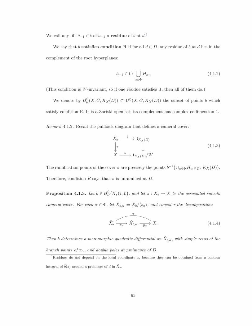
We call any lift a−1 ∈ t of a−1 a residue of b at d.1

We say that b satisfies condition R if for all d ∈ D, any residue of b at d lies in the

complement of the root hyperplanes:

a−1 ∈ t \⋃α∈Φ

Hα. (4.1.2)

(This condition is W -invariant, so if one residue satisfies it, then all of them do.)

We denote by B♦R(X,G,KX(D)) ⊂ B♦(X,G,KX(D)) the subset of points b which

satisfy condition R. It is a Zariski open set; its complement has complex codimension 1.

Remark 4.1.2. Recall the pullback diagram that defines a cameral cover:

Xb tKX(D)

X tKX(D)/W.

b

π

b

(4.1.3)

The ramification points of the cover π are precisely the points b−1(∪α∈ΦHα×C×KX(D)

).

Therefore, condition R says that π is unramified at D.

Proposition 4.1.3. Let b ∈ B♦R

(X,G,L), and let π : Xb → X be the associated smooth

cameral cover. For each α ∈ Φ, let Xb,α := Xb/〈sα〉, and consider the decomposition:

Xb Xb,α X.

π

πα pα(4.1.4)

Then b determines a meromorphic quadratic differential on Xb,α, with simple zeros at the

branch points of πα, and double poles at preimages of D.

1Residues do not depend on the local coordinate x, because they can be obtained from a contour

integral of b(z) around a preimage of d in Xb.

65

Proof. We have the following commutative diagram, in which the horizontal arrows in

the middle column are pullbacks of differential forms; all squares are fiber products.

Xb tπ∗KX(D) tπ∗α(KXb,α

(p∗αD)) π∗α(KXb,α(p∗αD))

Xb,α tp∗αKX(D)/〈sα〉 tKXb,α(p∗αD)/〈sα〉 KXb,α

(p∗αD)/Z2

X tKX(D)/W

b

πα

α

bα

pα

α

b

(4.1.5)

The composition of the middle horizontal arrows is an element of:

Γ(Xb,α,KXb,α

(p∗αD)/Z2

) ∼= Γ(Xb,α, (KXb,α

(p∗αD))⊗2). (4.1.6)

This is the desired quadratic differential. The branch points of πα are b−1α

(Hα×C∗KX(D)

),

which coincide with the zeros of the quadratic differential. Since we started with b ∈

B♦R

(X,G,KX(D)

), bα(Xb,α) intersects Hα ×C∗ KX(D) transversely, so all the zeros are

simple.

Definition 4.1.4. For each α ∈ Φ, we denote by:

ωb,α ∈ Γ(Xb,α, (KXb,α

(p∗αD))⊗2)

(4.1.7)

the quadratic differential obtained in Proposition 4.1.3. We denote by:

χb,α ∈ Γ(Xb,KXb,α

(p∗αD))

(4.1.8)

the linear differential on Xb obtained from composing the top horizontal arrows in diagram

4.1.5. It is immediate from the diagram that:

χb,α ⊗ χb,α = π∗αωb,α. (4.1.9)

Moreover, due to Condition R (Definition 4.1.1), ωb,α has a pole of order 2 at each d ∈ D.

66

Definition 4.1.5. Each χb,α determines an oriented foliation on Xb, by curves γ : R → Xb

satisfying: ∫ t1

t0

χb,α(γ(s)) ∈ R+. (4.1.10)

The oriented trajectories of χb,α are the maximal leaves of this foliation.

In Section 1.2, we already gave a teaser of how spectral networks arise from the

interaction between these oriented trajectories for different α ∈ Φ. Below we make this

precise. This is a generalization to arbitrary reductive G of the construction of WKB

spectral networks in [16] (for SL(n), GL(n)), [27] (type ADE), and of the Stokes graphs

in the literature on exact WKB analysis, e.g. [4, 1, 24, 22, 36] (these correspond to

networks for SL(n), and GL(n)).

Definition 4.1.6. From the data determined by b ∈ B♦R(X,G,KX(D)), we make the

WKB construction Wb, which consists of oriented curve segments on Xb called Stokes

curves, each labeled by an element of Φ. The curves are constructed algorithmically as

follows.

• A primary Stokes curve is a critical oriented trajectory of one of the χb,α; its label is

α. (We will prove in Lemma 4.1.15 that there are six primary Stokes curves starting

from each ramification point.)

• Let x ∈ Xb be any isolated intersection point of Stokes curves labeled by distinct

roots in some subset Cin ⊂ Φ. For each γ ∈ ConvNCin, a secondary Stokes curve �γ

starts at x; it is the unique leaf outgoing from x of the oriented foliation determined

by χb,γ . See Figure 4.1.

67

Figure 4.1: Stokes curves (solid) are segments of certain oriented trajectories (transpar-

ent). When Stokes curves labeled by α (blue) and β (yellow) intersect, oriented trajec-

tories of χb,γ1 , χb,γ2 , for γ1, γ2 ∈ ConvN{α,β}, are activated at the intersection point, and

become Stokes curves labeled by γ1, γ2 (green, khaki, respectively).

• Secondary Stokes curves are recursively created every time two or more of the ex-

isting Stokes curves intersect.

Define the joints of Wb to be the intersection points of Stokes curves; we denote by J

the set of joints.

Think of Wb as a directed graph, with vertex set R ∪ J , and a directed edge for each

connected component of Wb \ {R ∪ J}. We say that Wb is admissible if:

• no point in Xb \ π−1(D) is an accumulation point of the set J ;

• R ∩ J = ∅, i.e. Stokes curves do not run into ramification points;

• the directed graph corresponding to Wb is acyclic;

68

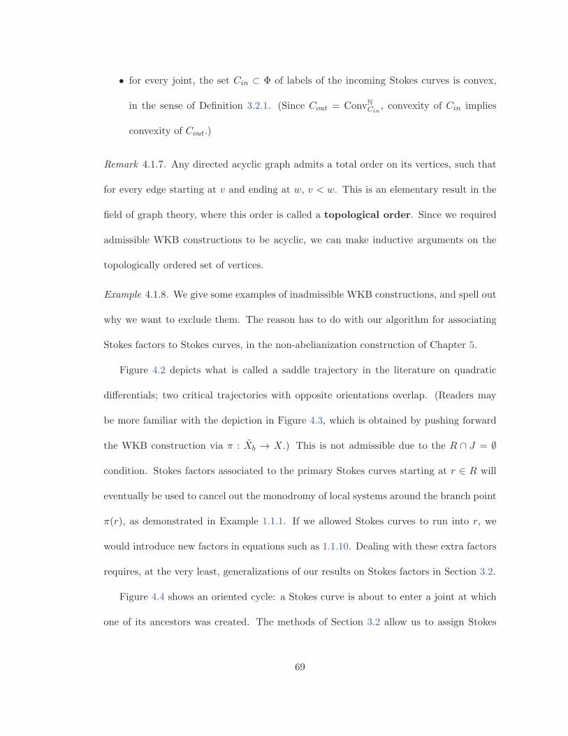
• for every joint, the set Cin ⊂ Φ of labels of the incoming Stokes curves is convex,

in the sense of Definition 3.2.1. (Since Cout = ConvNCin, convexity of Cin implies

convexity of Cout.)

Remark 4.1.7. Any directed acyclic graph admits a total order on its vertices, such that

for every edge starting at v and ending at w, v < w. This is an elementary result in the

field of graph theory, where this order is called a topological order. Since we required

admissible WKB constructions to be acyclic, we can make inductive arguments on the

topologically ordered set of vertices.

Example 4.1.8. We give some examples of inadmissible WKB constructions, and spell out

why we want to exclude them. The reason has to do with our algorithm for associating

Stokes factors to Stokes curves, in the non-abelianization construction of Chapter 5.

Figure 4.2 depicts what is called a saddle trajectory in the literature on quadratic

differentials; two critical trajectories with opposite orientations overlap. (Readers may

be more familiar with the depiction in Figure 4.3, which is obtained by pushing forward

the WKB construction via π : Xb → X.) This is not admissible due to the R ∩ J = ∅

condition. Stokes factors associated to the primary Stokes curves starting at r ∈ R will

eventually be used to cancel out the monodromy of local systems around the branch point

π(r), as demonstrated in Example 1.1.1. If we allowed Stokes curves to run into r, we

would introduce new factors in equations such as 1.1.10. Dealing with these extra factors

requires, at the very least, generalizations of our results on Stokes factors in Section 3.2.

Figure 4.4 shows an oriented cycle: a Stokes curve is about to enter a joint at which

one of its ancestors was created. The methods of Section 3.2 allow us to assign Stokes

69

Figure 4.2: Saddle trajectory, cameral

view.

Figure 4.3: Saddle trajectory, spectral

view.

factors to outgoing curves, based on the factors for incoming curves. Applying this in the

presence of oriented cycles would lead to circular reasoning.

Figure 4.4: An oriented cycle (labels of curves not shown).

Example 4.1.9. The “finite webs” that [16] consider also break the admissibility condition.

In Figures 4.5 - 4.6, we show finite webs for g = sl3, where α, β are simple roots (see the

root system A2 in Figure 3.2), and γ = −α− β.

The webs are not admissible because there are Stokes curves running into ramification

points, and because each double line creates an oriented cycle.

Definition 4.1.10. Let Wb be an admissible WKB construction. We call Wb a WKB

70

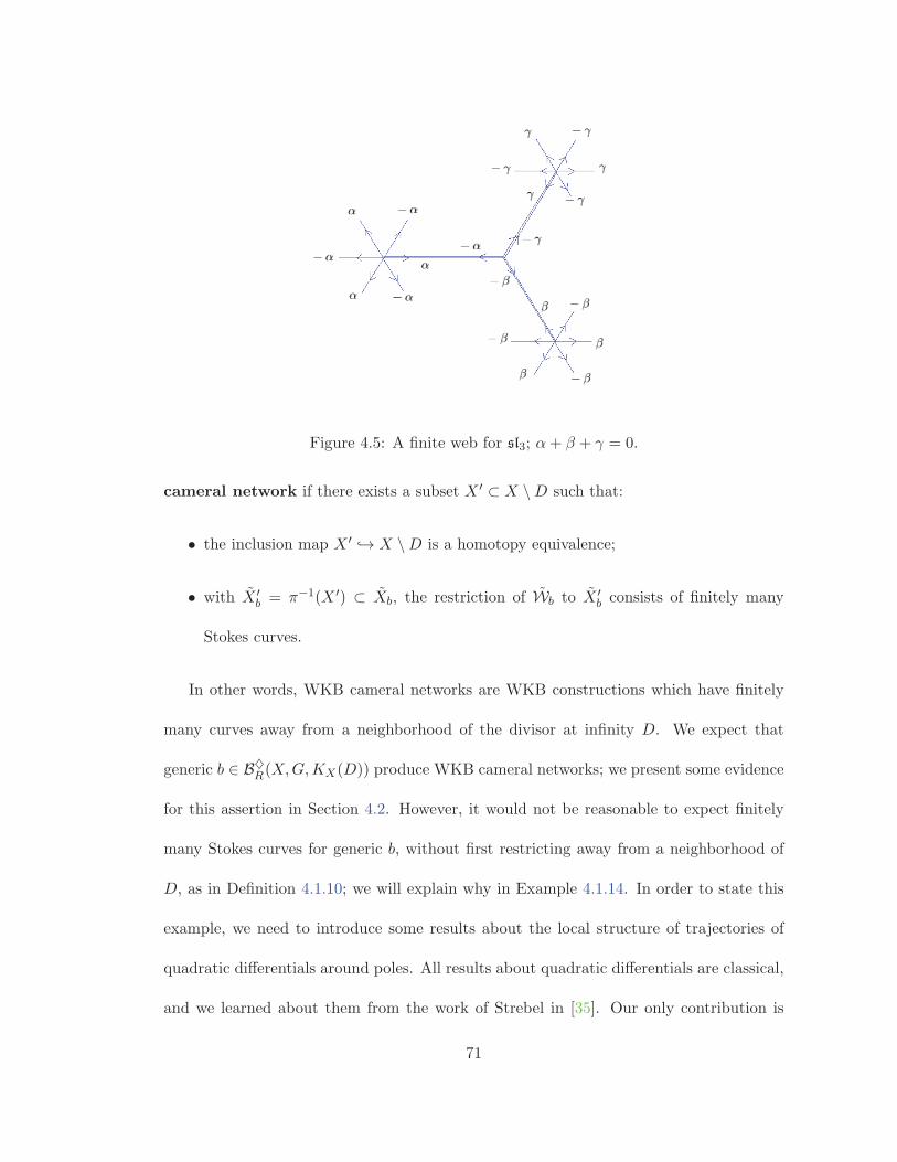
Figure 4.5: A finite web for sl3; α+ β + γ = 0.

cameral network if there exists a subset X ′ ⊂ X \D such that:

• the inclusion map X ′ ↪→ X \D is a homotopy equivalence;

• with X ′b = π−1(X ′) ⊂ Xb, the restriction of Wb to X ′

b consists of finitely many

Stokes curves.

In other words, WKB cameral networks are WKB constructions which have finitely

many curves away from a neighborhood of the divisor at infinity D. We expect that

generic b ∈ B♦R(X,G,KX(D)) produce WKB cameral networks; we present some evidence

for this assertion in Section 4.2. However, it would not be reasonable to expect finitely

many Stokes curves for generic b, without first restricting away from a neighborhood of

D, as in Definition 4.1.10; we will explain why in Example 4.1.14. In order to state this

example, we need to introduce some results about the local structure of trajectories of

quadratic differentials around poles. All results about quadratic differentials are classical,

and we learned about them from the work of Strebel in [35]. Our only contribution is

71

Figure 4.6: A more complicated finite web for sl3; α+ β + γ = 0.

deducing the implications of these results for WKB cameral networks.

Lemma 4.1.11 (Section 6.3 in [35]). Let L = KX(D), and ω ∈ Γ(X,L⊗2

)a meromorphic

quadratic differential. For every d ∈ D, there exists a local coordinate t centered at d such

that:

ω(t) = cddt⊗ dt

t2. (4.1.11)

Moreover, cd ∈ C× is independent of the choice of coordinate t.

Proof. Expand ω in a power series around d ∈ D:

ω(z) =

( ∞∑i=−2

aizi

)dz ⊗ dz. (4.1.12)

Strebel, in Theorem 6.3 of [35], defines a holomorphic function t = t(z), as an explicit

power series in the coefficients ai with non-zero radius of convergence, such that 4.1.11

holds. We have cd = a−2 – this coefficient is independent on the choice of coordinate,

because it is determined by a contour integral of√ω around d.

72

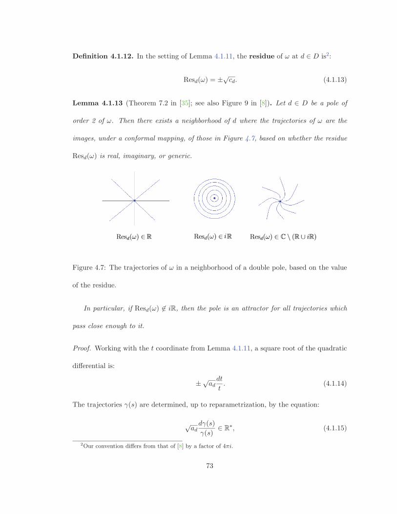
Definition 4.1.12. In the setting of Lemma 4.1.11, the residue of ω at d ∈ D is2:

Resd(ω) = ±√cd. (4.1.13)

Lemma 4.1.13 (Theorem 7.2 in [35]; see also Figure 9 in [8]). Let d ∈ D be a pole of

order 2 of ω. Then there exists a neighborhood of d where the trajectories of ω are the

images, under a conformal mapping, of those in Figure 4.7, based on whether the residue

Resd(ω) is real, imaginary, or generic.

Figure 4.7: The trajectories of ω in a neighborhood of a double pole, based on the value

of the residue.

In particular, if Resd(ω) �∈ iR, then the pole is an attractor for all trajectories which

pass close enough to it.

Proof. Working with the t coordinate from Lemma 4.1.11, a square root of the quadratic

differential is:

±√addt

t. (4.1.14)

The trajectories γ(s) are determined, up to reparametrization, by the equation:

√addγ(s)

γ(s)∈ R∗, (4.1.15)

2Our convention differs from that of [8] by a factor of 4πi.

73

which has the solution:

γ(s) = γ(0) exp (R∗√ads) . (4.1.16)

If√ad ∈ R, then γ(s) are radial rays. If

√ad ∈ iR, then γ(s) are circles centered at

d. In the generic case√ad �∈ R ∪ iR, γ(s) are logarithmic spirals.

The transformation z �→ t(z) is conformal. So, in any other coordinate, the trajectories

are conformal images of the ones in Figures 4.7.

Example 4.1.14. Let Wb be a WKB construction, and consider two Stokes curves �α, �β

labeled by α, β ∈ Φ, in a neighborhood of d ∈ D. Modulo orientation, they are the

preimages in Xb of trajectories of ωb,α, ωb,β , respectively. So, assuming that the residues

of ωb,α, ωb,β at d are generic and different, �α, �β are logarithmic spirals with different

slopes3, and one end converging to the pole. Assume that the orientation of �α, �β is

towards the pole. Then �α, �β intersect infinitely many times as they spiral towards the

pole. If it happens that α + β ∈ Φ, then each intersection spawns a new Stokes curve

labeled by α + β; the situation is depicted in Figure 4.8. Gaiotto, Moore and Neitzke

noticed this accumulation of joints at a pole; see figure 17 in their paper [16].

In the remainder of this section, we give some details about the structure of WKB

cameral networks locally around a ramification point or a joint on Xb.

Lemma 4.1.15. Assume that Wb is a WKB cameral network, and let r ∈ Xb be a

ramification point of the covering map π : Xb → X. Then there are six Stokes curves

starting from r. Moreover, there exists α ∈ Φ, uniquely determined up to sign, such that

the lines are labeled by α and −α, in alternating fashion, as shown in Figure 4.9.

3By “slope” of a logarithmic spiral we mean the phase of√ad from equation 4.1.16.

74

Figure 4.8: Two Stokes curves labeled by α, β (blue, black, respectively) spawn infinitely

many curves labeled by α+ β (red).

Figure 4.9: Stokes curves near a ramification point.

Proof. Due to admissibility, the only Stokes curves incident to r are the primary curves

produced there. Up to orientation, they are the inverse images, by πα : Xb → Xb,α, of

critical trajectories of the quadratic differential ωb,α, for some α ∈ Φ. Specifically, we want

the critical trajectories of ωb,α starting from a simple zero at πα(r); this means b(r) ∈ Hα.

For b ∈ B♦(X,G,L), there is a unique hyperplane on which b(r) lies – this determines α

up to sign.

There are three critical trajectories of ωb,α starting at r, because of the computation

75

done in Example 1.2.4. Pulling back to Xb via the 2:1 covering map πα, we obtain six

Stokes curves, oriented as in Figure 1.7. Notice that only three of them are oriented out

of r, thus giving Stokes curves labeled by α. The other three are oriented out of r when

regarded as trajectories of ωb,−α, so they are labeled by −α.

Definition 4.1.16. Let x ∈ J be a joint of a WKB cameral network Wb. We say that

Wb is convexity-preserving at x if the following condition holds. For each triple of

outgoing Stokes curves labeled by α, α + β, β ∈ Φ, denote by vα, vα+β , vβ ∈ TxXb, their

tangent vectors at x, well-defined up to scaling by R+. Then vα+β is contained in the

cone spanned by vα, vβ . See Figure 4.10.

More formally, the condition is that there exist cα, cβ ∈ R+ such that vα+β = cαvα +

cβvβ . The fullfillment of this condition clearly does not depend on rescaling the vectors

by R+.

Figure 4.10: The tangent vector vα+β is contained in the cone (shaded) spanned by vα,

vβ .

Lemma 4.1.17. WKB cameral networks are convexity-preserving at every joint x ∈ J .

Proof. For each γ ∈ {α, α+ β, β}, saying that vγ is tangent to a Stokes curve labeled by

γ means that:

γ(bx(vγ)

) ∈ R+, (4.1.17)

76

with b as in diagram 4.1.5, and bx : TxXb → t its evaluation at x. Since the result of this

lemma is independent of rescaling vγ by R+, we may as well assume that:

γ(bx(vγ)

)= 1. (4.1.18)

Moreover, since TxXb is 1-dimensional over C, there exist ηα, ηβ ∈ C∗ such that:

vα = ηαvα+β ,

vβ = ηβvα+β .

Then:

1 = (α+ β)(ax(vα+β)

)= α

(ax(vα+β)

)+ β

(ax(vα+β)

)= η−1

α α(ax(vα)

)+ η−1

β β(ax(vβ)

)= η−1

α + η−1β .

Consequently, η−1α + η−1

β = 1. Then, using the fact that ηη = |η|2, for all η ∈ C:

1

|ηα|2 vα +1

|ηα|2 vβ =1

|ηα|2 ηαvα+β +1

|ηα|2 ηβvα+β

= (η−1α + η−1

β )vα+β

= vα+β .

So we can take cα = 1/|ηα|2 and cβ = 1/|ηβ |2.

Remark 4.1.18. An immediate corollary of Lemma 4.1.17 is that, if the outgoing Stokes

curves at some joint x ∈ J ar labeled by a planar subset Cout ⊂ Φ, then the ordering of

these curves respects the ordering of the roots in the plane. For example, let α, β be the

77

short and long root of g2, respectively. Figure 4.11 depicts a possible pattern of outgoing

Stokes curves, labeled by Cout = ConvNα,β ; compare to the G2 root system from Figure

3.4.

Figure 4.11: Ordering of outgoing Stokes curves respects the ordering of the planar set of

labels.

When listing admissibility requirements in Definition 4.1.6, we included a convexity

property of the set Cin ⊂ Φ of labels of incoming Stokes curves at every joint. This

convexity assumption is needed for the results about Stokes factors from section 3.2, such

as Theorem 3.2.21. We believe that the convexity property follows from the acyclicity

property, which is another item on the list of admissibility requirements. But to prove

this, we seem to need the following fact about root systems.

Conjecture 4.1.19. Assume that {γi}ki=0 ⊂ Φ+ is a subset of roots, positive for a choice

of polarization Φ+. Assume that they satisfy a linear relation:

n0γ0 =

k∑i=1

niγi, (4.1.19)

with all ni ∈ N. Finally, assume that this relation is minimal, in the sense that, if there

is a tuple (m0, . . . ,mk) ∈ Nk+1, with mi ≤ ni for all i, and:

m0γ0 =

k∑i=1

miγi, (4.1.20)

78

then (m0, . . . ,mk) = (n0, . . . , nk).

Then at least one of the coefficients in {ni}ki=0 is equal to 1.

We can prove this conjecture in the following cases:

1. For root systems of type A, the proof of Lemma 3.2.6 shows that, in a minimal

linear relation between positive roots, all coefficients are 1.

2. For the planar root systems B2 and G2, the result is obvious from Figures 3.3–3.4.

Lemma 4.1.20. Let Wb be a WKB cameral network for a Lie algebra g whose root system

satisfies Conjecture 4.1.19. Let x ∈ J be a joint. Then the set Cin of labels of the incoming

Stokes curves at x is a convex subset of Φ.

Proof. Assume that Cin is not convex, and let C ′in ⊂ Cin be the smallest subset which is

not convex. Then:

• For all γ ∈ C ′in, the set C ′

in \ γ is convex.

• By Definition 3.2.1, for all γ ∈ C ′in, −γ ∈ ConvC′

in\{γ}.

We claim that there exists γ0 ∈ C ′in, such that −γ0 ∈ ConvNC′

in\{γ0}. As a consequence

of the claim, there is an outgoing Stokes curve labeled by −γ0 at the joint x. Its underlying

curve, and the underlying curve of the incoming Stokes curve labeled by γ0, are the same,

but they have opposite orientations. This “double wall” creates an oriented cycle in Wb,

contradicting admissibility.

To prove the claim, choose any γ0 ∈ C ′in, and let {γ1, . . . , γn} be an ennumeration of

C ′in \ {γ0}. Then:

− γ0 =

k∑i=1

ciγi, ci ∈ [0,∞). (4.1.21)

79

In fact, we can take ci ∈ Q. This is because each γi is an integral linear combination

of simple roots, so the ci are a solution to a system of linear equations with integral

coefficients. Then, multiplying 4.1.21 by the lowest common multiple of all denominators,

we obtain a linear relation with integral coefficients:

n0(−γ0) =k∑

i=1

niγi, ni ∈ N. (4.1.22)

Moreover, by the convexity of C ′in \ {γ0}, there is a polarization of the root system, such

that −γ0 and all other γi are positive.

Applying the result of Conjecture 4.1.19, and decreasing the coefficients in 4.1.22 if

the relation is not already minimal, we obtain that one of the ni is equal to 1. If n0 = 1,

then −γ0 ∈ ConvNC′in\{γ0}, and we are done. If one of the other nj is 1, then rewrite the

linear relation as:

− γj =∑i �=j

niγi, (4.1.23)

and swap the indices of γj and γ0.

Remark 4.1.21. In Section 9 of their paper [16], Gaiotto, Moore and Neitzke observe that

certain applications, such as non-abelianization, make use of the topological structure of

spectral networks, without relying on their analytic structure, given by the differential

equations that prescribe the trajectories. They introduce “generic spectral networks” in

[16], as objects with just as much structure as non-abelianization requires.

Motivated by this point of view, in [23] we introduced what we think is a minimal list

of axioms for Stokes curves, in order to make non-abelianization possible. We called the

resulting topological objects “abstract cameral networks”.

80

4.2 How generic are WKB cameral networks?

We begin this section by reviewing some facts about the global structure of trajectories,

following the book [35] by Strebel and the paper [8] by Bridgeland and Smith. Then we

will use these facts to comment on the genericity of admissible WKB constructions and

WKB cameral networks – see Conjecture 4.2.10 and Proposition 4.2.13 below.

Definition 4.2.1 (Section 3.4 in [8]). Let ω be a meromoprhic quadratic differential on

a compact Riemann surface.

• The finite critical points of ω, denoted by Crit<∞(ω), are the zeros and poles of

order 1 of ω. 4

• The infinite critical points of ω, denoted by Crit∞(ω), are the poles of order ≥ 2

of ω.

We call a trajectory of ω:

1. a saddle trajectory if it approaches finite critical points at both ends (see Figure

4.3);

2. a separating trajectory if it approaches a finite critical point at one end, and an

infinite critical point at the other;

3. a closed trajectory if it is a closed curve;

4. a recurrent trajectory if it is dense at every point in its closure;

4This definition is motivated by the fact that trajectory segments which run into a finite critical point

have finite length, measured in the metric determined by ω. See section 5.3 in [35].

81

5. a generic trajectory if it approaches infinite critical points at both ends.

Proposition 4.2.2 (Sections 9-11 in [35]). Let ω be a meromorphic quadratic differential

on a compact Riemann surface. Then every trajectory of ω is of one of the 5 types listed

above.

Proposition 4.2.2 implies that, if a trajectory is dense at a regular point of ω, then it

is recurrent, i.e. dense at every point in its closure. In this case, it must be a space-filling

curve in some open subset of X.

Example 4.2.3. Consider the meromorphic quadratic differential on P1:

ω(x) =x(x− 4)

(x− 1)2(x− 2)2(x− 3)2dx⊗ dx. (4.2.1)

It has simple zeros at 0, 4 and double poles at 1, 2, 3. Away from ∞ ∈ P1, the trajectory

structure of ω is sketched in Figure 4.12.

The solid curves are separating trajectories; there are three of them for each simple

zero. They subdivide P1 into 3 regions, each of which is filled by generic trajectories

having both ends on a double pole.

Example 4.2.4 (§12.1 in [35]). Let X be the compact torus C/(Z + iZ). Consider holo-

morphic quadratic differentials on X, ω(x) = f(x)dx ⊗ dx. Then f(x) is a holomorphic

function on the compact torus, hence equal to a constant c. Up to scaling by R∗, tangent

vectors to the trajectories are c−1/2∂x. We consider two cases:

1. If c ∈ R+, then the trajectories are horizontal on C, hence closed curves on the

torus.

82

Figure 4.12: Separating trajectories (solid) and generic trajectories (transparent), for the

quadratic differential from equation 4.2.1. The three blue circles are the double poles.

2. If �(c−1/2)/�(c−1/2) is irrational, then the trajectories are space-filling curves, dense

at every point of the torus.

Definition 4.2.5. We say that a quadratic differential is saddle-free if it has no saddle

trajectories. We say that b ∈ B♦R(X,G,L) is saddle-free if for all α ∈ Φ, the quadratic

differential ωb,α induced by b on Xb,α is saddle-free.

The next results show that, under mild hypotheses on the number and type of crit-

ical points, saddle-free quadratic differentials form a dense open subset in the space of

quadratic differentials; moreover, all their trajectories are either separating (finitely many)

or generic (all others), as was the case in Example 4.2.3.

Proposition 4.2.6 (Sections 9-11 of [35]; Lemma 3.1 in [8]; Section 6.3 in [17]). Let ω be

a saddle-free meromorphic quadratic differential, with at least one finite and one infinite

critical point. Then ω has no recurrent or closed trajectories.

Proof. Strebel proves that closed trajectories never come alone, but in families whose

union is open; he calls these ring domains (Theorem 9.4 in [35]). For example, the case

83

Resd(ω) ∈ iR from Figure 4.7 depicts a ring domain. Similarly, recurrent trajectories

span an open set called a spiral domain. Strebel then proves that the boundaries of both

ring domains and spiral domains necessarily include a saddle trajectory, except for two

situations (Corollary 2 to Theorem 11.2 in loc. cit.):

• A ring domain which contains all but finitely many points (e.g. a compact torus, or

P1 \ {0,∞} can be foliated by circles). This is forbidden by the assumption that ω

has at least one finite critical point.

• A spiral domain which is dense on the Riemann surface. This is forbidden by the

existence of an infinite critical point. Indeed, due to Proposition 4.1.13, poles of

order 2 have a neighborhood in which no trajectory can be recurrent. Strebel proves

in Theorem 7.4 of [35] that an analogous statement holds for all poles of order ≥ 2.

Definition 4.2.7 (§2.5 in [8]). For g, n ∈ N such that 2g−2+n > 0 let Quad(g, n) denote

the moduli stack (orbifold) of meromorphic quadratic differentials ω on a Riemann surface

of genus g with n punctures, such that:

• ω has a pole of order 2 at each puncture;

• ω has only simple zeros.

More precisely, let Mg,n denote the moduli stack of Riemann surfaces of genus g

and n punctures, and let Hg,n → Mg,n/Sn denote the vector bundle whose fiber over

(X, {p1, . . . , pn}) is:

H0(X,K⊗2

X (2p1 + · · ·+ 2pn)). (4.2.2)

84

Then Quad(g, n) is the Zariski open substack of Hg,n, consisting of sections with simple

zeros that avoid the pi.

Proposition 4.2.8 (Lemma 4.11 in [7]; see Theorem 1.4 in [2] for a statement involv-

ing higher-order poles). The subset U ⊂ Quad(g, n) consisting of saddle-free quadratic

differentials is open and dense in the classical topology. Moreover, the intersection of U

with every orbit of S1, acting on quadratic differentials as rescaling by eiθ, is dense in the

orbit.

Consequently, we can make the following statement about points in the Hitchin base.

Proposition 4.2.9. The subset of saddle-free points in B♦R(X,G,L) is open and dense

in the classical topology.

Proof. Diagram 4.1.5, provides, for each α ∈ Φ, a map:

B♦R

(X,G,KX(D)

)Quad(gα, n),

b ωb,α,

ωα

(4.2.3)

where n is the degree of p∗α(D), and gα is the genus of Xb,α; both numbers are constant

as b varies in B♦R(X,G,L). (Note that, using Propositions 2.3.6 and 2.3.7, Xb is smooth

and connected; then the same holds for Xb,α.)

According to Proposition 4.2.8, saddle-free differentials in Quad(gα, n) form an open

subset Uα. Then saddle-free points of B♦R(X,G,L) also form the open subset:

U :=⋂α∈Φ

ω−1α (Uα). (4.2.4)

It remains to prove that U is dense. Clearly the image of ωα is a disjoint union of

S1 orbits: under b �→ eiθb, we have ωb,α �→ e2iθωb,α. By Proposition 4.2.8, Uα is dense in

85

each S1 orbit. Therefore ω−1α (Uα) is dense in B♦

R(X,G,L). Taking the intersection over

all α ∈ Φ, U is also dense.

Conjecture 4.2.10. The subset of b ∈ B♦R(X,G,L) such that Wb is admissible is open

and dense in the classical topology.

Proposition 4.2.9 is a partial result in the direction of this conjecture. For a full proof,

we would need to argue that the following phenomena are also non-generic:

• oriented cycles such as the one in Figure 4.4;

• a Stokes curve � running into a ramification point r ∈ R, with the label of � not

necessarily equal to the root α such that b(r) ∈ Hα;

• joints accumulating at some point in Xb \ π−1(D).

Such arguments necessarily involve dealing with ωb,α for multiple α at the same time; we

do not carry them out.

However, being saddle-free is enough to guarantee the following desirable property for

the WKB construction.

Proposition 4.2.11. If b ∈ B♦0 (X,G,L) is saddle-free, then the limit set of each Stokes

curve � in Wb consists of only two points:

• the finite critical point or joint where � is created;

• the infinite critical point where � ends.

Proof. Each Stokes curve is a subset of a (not necessarily critical) trajectory of ωb,α, for

some α. By assumption, each ωb,α is saddle-free. Then Proposition 4.2.6 guarantees that

86

all trajectories are either separating or generic. In particular, they all end at an infinite

critical point.

Putting together Propositions 4.2.9 and 4.2.11, we obtain:

Corollary 4.2.12. There is a dense open subset of the Hitchin base, consisting of points

b such that for all Stokes curves � in the associated WKB construction Wb, the limit set

of � consists of two critical points, one initial and one final.

Finally, we prove that, under the admissibility hypotheses made in Definition 4.1.6,

WKB constructions have finitely many Stokes curves away from a neighborhood of π−1(D).

Proposition 4.2.13. Assume that Wb is admissible. Then Wb is a WKB cameral net-

work.

Proof. We must prove that the restriction of Wb away from a small neighborhood of

π−1(D) contains finitely many Stokes curves. The strategy is to find a contractible neigh-

borhood Ud of each d ∈ D, such that the (possibly infinitely many, as in Example 4.1.14)

Stokes curves produced in Ud never leave Ud.

For admissible WKB constructions Wb, and for all α ∈ Φ, the quadratic differentials

ωb,α are saddle-free. From Proposition 4.2.6, ωb,α have no closed trajectories. Then, due

to Lemma 4.1.13, we have Resd(ωb,α) �∈ R for all d ∈ D. Then there exists a contractible

neighborhood Uα,d of d such that the trajectories of ωb,α passing through Uα,d have one

end at d, and cross the boundary of Uα,d only once.

Define Ud = ∩α∈Φπ∗α(Ud,α) ⊂ Xb. The Stokes curves passing through Ud are inverse

images by some πα of the trajectories discussed in the previous paragraph. Therefore,

87

they have one end at d, and pass through the boundary of Ud at most once. We want to

prove that all of them are oriented towards d, so that they never exit Ud.

This is clear for primary Stokes curves – by definition, they are created at a ramifica-

tion point of π, outside Ud, so they must end at d. The argument for secondary Stokes

curves is by induction on the topologically-ordered set of joints (see Remark 4.1.7); its va-

lidity relies on the acyclicity condition for admissible WKB constructions. So let {xn}n∈N

be a topologically-ordered ennumeration of J . The primary Stokes curves provide the base

case for the induction. Assume, then, that all Stokes curves created at {x1, . . . , xn−1},

for some n ∈ N, are oriented towards d. We want to prove the same for xn. Due to

the topological order and the inductive hypothesis, the incoming Stokes curves at xn are

oriented towards d. Lemma 4.1.17 then guarantees that tangent vectors to the outgoing

curves are contained in the real cone spanned by tangent vectors to the incoming curves.

Therefore, the outgoing curves at xn must also be oriented towards d.

It remains to prove that there cannot be infinitely many secondary Stokes curves

produced outside of the opens Ud. Note that the subset:

X ′b := Xb \ ∪d∈DUd (4.2.5)

is compact; as such, if there are infinitely many joints inside it, they must have an ac-

cumulation point in X ′b. Our hypothesis explicitly forbids this, so there must be finitely

many joints inside X ′b. Since the number of secondary Stokes curves produced at a joint is

bounded above by |Φ|, we conclude that there are finitely many secondary Stokes curves

produced inside X ′b.

The subsets Ud are contractible; by shrinking them if necessary, we can assume they

88

are disjoint. Then the inclusion X ′b ↪→ Xb \ π−1(D) induces a homotopy equivalence.

4.3 Equivariance and spectral networks

Ultimately, to perform non-abelianization we need networks on X, and not on Xb. In this

section we describe the passage from WKB cameral networks, which are objects on Xb,

to spectral networks, which are objects on X.

Lemma 4.3.1. WKB cameral networks are W -equivariant, in the following sense. For

every w ∈ W , and Stokes curve � ⊂ Xb labeled by α ∈ Φ, the subset w(�) ⊂ Xb5 is a

Stokes curve labeled by w(α).

Proof. The action ofW on t∗ � α, is dual to that on t. Then, for every w ∈W and r ∈ R,

b(w(r)

) ∈ Hw(±α) ×C∗ KX(D). Therefore, the primary Stokes curves starting at w(r) are

labeled by w(α).

The W -equivariance of b implies that:

χwα = (w(α)⊗ 1) ◦ b = (α⊗ 1) ◦ wb = w∗χα. (4.3.1)

For the oriented trajectories, this means w(�α) = �w(α).

Whenever �1, �2 intersect at x ∈ J , then w(�1), w(�2) intersect at w(x). The restricted

convex hulls satisfy ConvNαw(�1),w(�2)= w

(ConvNα�1,�2

). Therefore, the production of sec-

ondary Stokes curves is W -equivariant.

Definition 4.3.2. Let Wb be a WKB cameral network. The associated WKB spectral

network Wb is the following union of oriented, labeled curves on X:

5When we write w(�), we are using the action of the Weyl group on the cameral cover Xb.

89

• As oriented curves, Wb = π∗Wb.

• The label of � ∈ Wb is a locally constant section ψ� of HomW (Xb|�,Φ). It maps any

preimage � of � to the root which labels �.

Remark 4.3.3. WKB cameral networks have six Stokes curves are created from each

ramification point r ∈ R (Lemma 4.1.15). The restriction of π : Xb → X to a small

neighborhood of r has degree 2, so theW -equivariance proved in Lemma 4.3.1 ensures that

the corresponding spectral network has three Stokes curves outgoing from each branch

point. This agrees with the constructions of spectral networks in [16], [27].

To analyze the relationship between the labeling of our spectral networks and the

labeling of spectral networks in [16], [27], we introduce the following definition.

Definition 4.3.4. Let x ∈ X \ P . A W-framing of the cameral cover π : Xb → X at x

is the data of a local trivialization φx : π−1(x) ∼=W .

Remark 4.3.5. A W -framing φx at any x ∈ �, for � ∈ W, gives a mapping:

HomW (Xb|�,Φ) → Φ,

ψ� �→ ψ�

(φ−1x (1W )

).

(4.3.2)

Thus, each choice of trivialization gives a way to label curves in the spectral network by

elements of Φ. If x is chosen close to a branch point p, then we can parallel transport

a trivialization φx along a loop around p, to obtain a labeling of the 3 outgoing Stokes

curves at p by α,−α, α, for some α ∈ Φ. Note, however, that this process is necessarily

discontinuous, because the cover has monodromy around p.

The spectral cover used by the earlier works [16], [27] is trivialized away from a system

of branch cuts, and curves in the spectral network are labeled by roots of g. The map in

90

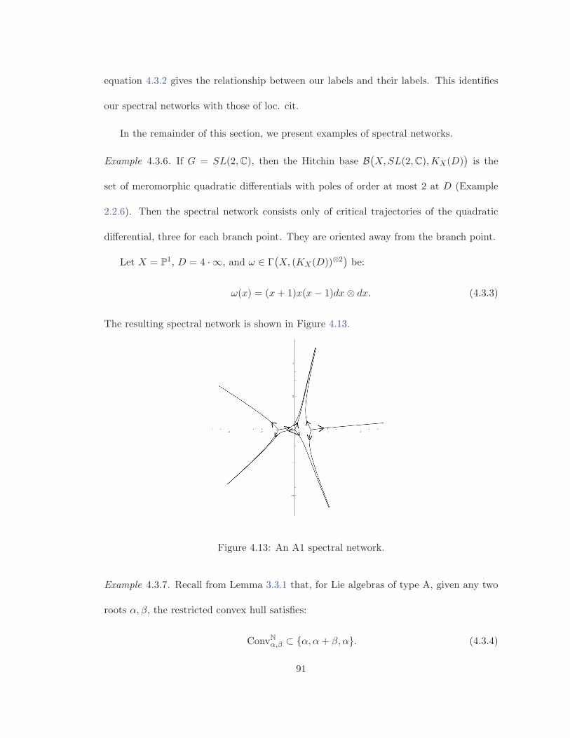
equation 4.3.2 gives the relationship between our labels and their labels. This identifies

our spectral networks with those of loc. cit.

In the remainder of this section, we present examples of spectral networks.

Example 4.3.6. If G = SL(2,C), then the Hitchin base B(X,SL(2,C),KX(D))is the

set of meromorphic quadratic differentials with poles of order at most 2 at D (Example

2.2.6). Then the spectral network consists only of critical trajectories of the quadratic

differential, three for each branch point. They are oriented away from the branch point.

Let X = P1, D = 4 · ∞, and ω ∈ Γ(X, (KX(D))⊗2

)be:

ω(x) = (x+ 1)x(x− 1)dx⊗ dx. (4.3.3)

The resulting spectral network is shown in Figure 4.13.

Figure 4.13: An A1 spectral network.

Example 4.3.7. Recall from Lemma 3.3.1 that, for Lie algebras of type A, given any two

roots α, β, the restricted convex hull satisfies:

ConvNα,β ⊂ {α, α+ β, α}. (4.3.4)

91

See Figure 3.2. As such, there is at most one new Stokes curve generated at each joint.

Consider G = SL3(C), which has the root system A2; X = P1; D = ∞. Take

b ∈ B♦R(X,G,L) corresponding to the characteristic polynomial:

f(λ, x) = λ3 + 3λ+ 2ix = 0. (4.3.5)

The discriminant of f :

− 4 · 33 − 27(2ix)2 (4.3.6)

vanishes at x = ±1. These are the branch points of the associated cameral cover. We

choose a pre-image r+1, r−1 of each branch point in the cameral cover. Let ±α,±β ∈ Φ

denote the roots such that b(r+1) ∈ Hα, b(r−1) ∈ Hβ . The cameral network has 6 primary

Stokes curves starting at r+1, labeled by ±α, and 6 starting at r−1, labeled by ±β. There

are two pairs of curves labeled by α, β which intersect on Xb, producing curves labeled

by α + β; by equivariance, two analogous intersections happen for pairs w(α), w(β), for

all w ∈W .

Pushing forward the network to X, we obtain the result in Figure 4.14.

This example first appeared in [4], which was, to the best of our knowledge, the first

source to mention new Stokes curves at the intersections of old ones. The context was

WKB analysis of solutions to differential equations.

92

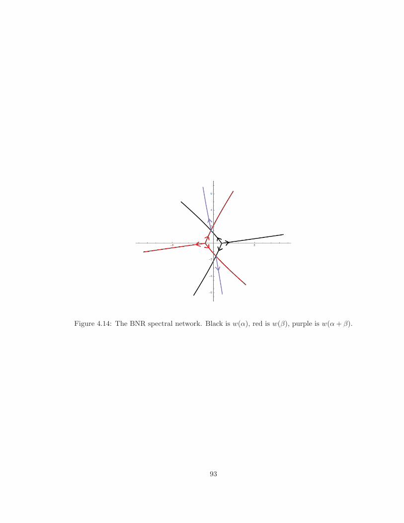
Figure 4.14: The BNR spectral network. Black is w(α), red is w(β), purple is w(α+ β).

93

Chapter 5

The non-abelianization map

In this chapter we introduce the moduli spaces involved in non-abelianization, and provide

the non-abelianization construction. Rather than local systems on the closed Riemann

surface X, we will consider local systems on certain oriented real blowups1 of X. If E

is a reduced, effective divisor on X, then X◦E denotes the oriented real blowup at every

point in the support of E. Specifically, in this chapter we will consider:

• E = D, where D is the divisor at infinity;

• E = D + P , where P is the branch divisor of the cover π;

• E = D + P + J , where J are the joints of a spectral network.

Throughout the chapter, we work with a fixed b ∈ B♦R(X,G,KX(D)), and we suppress b

from the notation for the cameral cover, which we denote by X. We will also use X◦D+R ,

where R is the ramification divisor of π, and we omit the distinction between D and its

1Concretely, an “oriented real blowup at x ∈ X” means replacing x with a boundary circle S1x, which

inherits an orientation from the orientation of X.

94

preimage π−1(D). (Due to Condition R, introduced in Definition 4.1.1, π is unramified

over D.) The restriction π◦ : X◦D+R → X◦D+P of π is unramified, hence a principal

W -bundle.

In section 5.1 we introduceN -shifted, weaklyW -equivariant T -local systems on X◦D+R

and show their equivalence to those N -local systems on X◦D+P which extend the cameral

cover X. In section 5.2, we introduce a restriction on the monodromy of these T - and

N -local systems, which we call the S-monodromy condition. Finally, in section 5.3 we

provide the non-abelianization construction, giving a proof of Theorem 1.1.5.

5.1 From T-local systems to N-local systems

In the case G = GL(n,C), the spectral construction described in Section 2.3 works by

pushing forward a line bundle L on the n-sheeted spectral cover π : X → X, to obtain

a rank n vector bundle on X. Away from the branch points of the cover, we obtain

a reduction of structure of π∗(L) to a NGL(n,C)-bundle, by considering automorphisms

which preserve the following decomposition, for x ∈ X not a branch point:

π∗(L)|x ∼=⊕

x∈π−1(x)

Lx. (5.1.1)

TGL(n,C)∼= (C∗)n acts by scaling on each summand, while elements in non-trivial cosets

of NGL(n,C) also permute the factors.

In [12], Donagi and Gaitsgory give an analogue of this for reductive algebraic groups

G, using the cameral cover X instead of the spectral cover X. In the special case of an

unramified cover such as π◦ : X◦D+R → X◦D+P , their work relates certain N -bundles on

X◦D+P to “N -shifted, weakly W -equivariant” T -bundles on X◦D+R . In this section, we

95

introduce these ideas in the setting of local systems, where the unramified case of [12]

applies with no significant modifications. The result is Theorem 5.1.7.

In a nutshell, the strategy is to:

• Take the direct image π◦∗(L) of a T -local system on X◦D+R .

• Find conditions on L, such that π◦∗(L) is an N -local system.

Lemma 5.1.1. Let L ∈ LocT (X◦D+R). Let Aut(π◦∗(L)) denote the sheaf of automor-

phisms of the direct image π◦∗(L), seen as a sheaf on X◦D+P with the classical topology.

Then its sections over an open set U ⊂ X◦D+P are:

Aut(π◦∗(L))(U) ={(w, φ)

∣∣∣w ∈W,φ : w∗L|(π◦)−1(U)

∼=→ L|(π◦)−1(U)

}. (5.1.2)

Proof. Let Ui ⊂ (π◦)−1(U) be a homeomorphic preimage of U . Since π◦ has the structure

of a W -local system, for each 1 ≤ i, j ≤ |W |, there is a unique wij ∈ W such that

wij(Ui) = Uj . An element of Aut(π◦∗(L))(U) is equivalent to:

• A choice of w ∈W , such that w∗(L|U1) is a sheaf over Ul, for some l.

• An isomorphism φ1 : w∗L|U1

∼= L|Ul.

Then, for values of j other than 1, w∗(L|Uj) is a sheaf over ww1jw

−1(Ul), and φ1 deter-

mines an isomorphism:

φj := (ww1jw−1)∗(φ1) : w∗(L|Uj

) ∼= L|ww1jw−1(Ul). (5.1.3)

The set of all φl provides φ as in 5.1.2.

In order for π◦∗(L) to be an N -local system, we need an identification of Aut(π◦∗(L))with the constant sheaf N . Such an identification does not exist for arbitrary L; we

96

need to impose a constraint on L (weak W -equivariance) and equip it with extra data

(N -shifting).

Definition 5.1.2 (cf. Definition 5.7 of [12]). We call a T -local system L on X◦D+R

weakly W -equivariant if for each U , the projection Aut(π◦∗(L))→W is surjective.

Let Homlc(X◦D+R , T ) denote the sheaf of locally constant morphisms X◦D+R → T .

Then AutX◦D+P (L) is part of a sequence of locally constant sheaves on X◦D+P , which is

exact on the right if and only if L is weakly W -equivariant:

1 Homlc(X◦D+R , T ) Aut(π◦∗(L)) W 1. (5.1.4)

Defining this sequence uses the fact that T is abelian, so we can globally identify auto-

morphisms of L on X◦D+R with locally constant maps X◦D+R → T .

Remark 5.1.3. The short exact sequence 5.1.4 splits if and only if L is W -equivariant.

In this case, we obtain an identification of Aut(π◦∗(L)) with the constant sheaf T �W .

This is not quite what we want, because N can be a non-split extension of W by T . For

example, N ∼= T � W for the groups GL(n,C), SL(2n + 1,C), SO(n,C), but not for

SL(2n,C) (see, for example, the introduction to [12]).

For general G, we need the following definition.

Definition 5.1.4 (cf. §6.2 in [12]). An N-shifted, weakly W -equivariant T -local

system on X◦D+R is a weakly W -equivariant T -local system L on X◦D+R , together with

a map γ : N → Aut(π◦∗(L)) making the following diagram commute:

1 T N W 1

1 Homlc(X◦D+R , T ) Aut(π◦∗(L)) W 1.

diag γ (5.1.5)

97

Definition 5.1.5. We define LocNT (X◦D+R) to be the moduli stack of N -shifted, weakly

W -equivariant T -local systems on X◦D+R . A more formal definition, in terms of fiber

products of stacks, can be found in [23]. We do not reproduce it here, because it is not

necessary for the understanding of the rest of this chapter.

We will prove that, if L ∈ LocNT (X◦D+R), then π◦∗(L) is an N -local system on X◦D+P .

The following definition specifies which N -local systems arise in this way.

Definition 5.1.6. Recall that π◦ : X◦D+R → X◦D+P is a W -local system. An N -local

system on X◦D+P which extends π◦ (or extends the cameral cover, when the partic-

ular cameral cover is clear from context) is an N -local system E , together with the data

of an isomorphism:

E/T ∼= X◦D+R . (5.1.6)

We denote by LocXN (X◦D+P ) the moduli space of N -local systems extending the cameral

cover. More formally, the relevant moduli space is:

LocXN (X◦D+P ) := LocN (X◦D+P )×LocW (X◦D+P ) {X◦D+R}. (5.1.7)

Theorem 5.1.7. Then there is an equivalence of categories between:

1. Weakly W -equivariant, N -shifted T -local systems L on X◦D+R ;

2. N -local systems which extend the cameral cover X◦D+R .

This gives an isomorphism of stacks:

LocNT (X◦D+R) ∼= LocXN (X◦D+P ). (5.1.8)

98

Proof. Let L be a weakly W -equivariant, N -shifted T -local system on X◦D+R , and define

E = π◦∗(L). Then the map γ : N → Aut(E) allows us to consider E as an N -local system.

Due to Diagram 5.1.4, there is an isomorphism of W -local systems:

E/T ∼= X◦D+R . (5.1.9)

Conversely, let E be an N -local system on X◦D+P which extends π◦. Then E → E/T ∼=

X◦D+R is a T -local system L on X◦D+R , on which the T -action comes from the inclusion

T ⊂ N . It is clear that π◦∗(E) ∼= L; the identification N ∼= Aut(E) provides the map

γ : N → Aut(π◦∗(L)), required by diagram 5.1.4.

The above constructions work in families, and their application to the universal fam-

ilies over the two stacks yields the stated isomorphism.

Being N -shifted, weakly W -equivariant imposes non-trivial monodromy constraints

on the T -local system. We give an example below, and we will elaborate on this point in

the next section.

Example 5.1.8. Consider G = SL(2), X = P1x, D = {∞} and X = P1

z, with the map

X → X given by z �→ z2. Then LocXN (X◦D+P ) ∼= (nT )/N , where n ∈ N is a representative

of the T -coset N \ T , and the map takes a local system to its monodromy around 0,

well-defined up to the adjoint action of N .

Now let L ∈ LocNT (X◦D+R). Then the monodromy of L around 0 is M2, where M is

the monodromy of π◦∗(L) around 0. By the previous paragraph, M ∈ (nT )/N ; for any

such element, a quick computation shows that M2 = −id.

Remark 5.1.9. In their version of non-abelianization in [16], Gaiotto, Moore and Neitzke

notice that they cannot work with honest local systems on the spectral cover, and consider

99

“twisted local systems” instead. The monodromy constraint for LocNT (X◦D+R) that we

obtained in Example 5.1.8 is a manifestation of the same phenomenon: we need to work

with T -local systems which have constrained, nontrivial monodromy around ramification

points.

5.2 The S-monodromy condition

We could attempt to define non-abelianization as a map2:

LocXN (X◦D+P ) LocG(X◦D+P ). (5.2.1)

However, this is not satisfactory: we would like the resulting G-local systems to extend

past the branch divisor P . To ensure this, we will construct a map from an appropriate

subspace of the source moduli space.

? LocG(X◦D)

LocXN (X◦D+P ) LocG(X◦D+P )

nonab

(5.2.2)

The goal of this section is to introduce the unknown space in the diagram above.

Definition 5.2.1. We say that E ∈ LocXN (X◦D+P ) satisfies the S monodromy con-

dition if, for each p ∈ P , the monodromy of E around S1p is contained in:⎛

⎝ ∐α∈Λp

nαTα

⎞⎠ /N, (5.2.3)

where Λp denotes the W -orbit of roots α such that b(p) ∈ Hα ×C∗ KX(D).

For Definition 5.2.1 to make sense,∐

α∈ΛpnαTα must be preserved by the adjoint

action of N . This is shown in Lemma 3.1.16.2See Remarks 5.3.7, 5.3.8.

100

Definition 5.2.2. We denote by LocX,SN (X◦D+P ) the moduli space of N -local systems

which extend the cameral cover π◦ and satisfy the S-monodromy condition.

More formally, we define:

LocX,SN (X◦D+P ) := LocXN (X◦D+P )×(

∏p∈P N/N)

∏p∈P

(( ∐α∈Λp

nαTα

)/N

), (5.2.4)

where the map LocXN (X◦D+P ) →∏p∈P N/N is restriction of local systems to the boundary

circles, and Λp is the W -orbit of α ∈ Φ such that b(p) ∈ Hα ×C∗ KX(D).

We provide a further point of view on the S-monodromy condition, which will be

useful in section 5.3.

Remark 5.2.3. By Lemma 3.1.14, conjugation by T preserves the subset nαTα of nαT , so

we obtain a map:

nαTα/T → nαT/T. (5.2.5)

Let E ∈ LocXN (X◦D+P ), and let p ∈ P . In the presence of a W -framing (Definition

4.3.4) at xp, for some xp on the boundary circle S1p , the monodromy of the cameral cover

E/T around S1p is identified with sα ∈ W , for some root α. Then, using the notation of

section 3.1, the monodromy of E around S1p is identified with an element of nαT/T . The

S-monodromy condition for N -local systems is the requirement that this element be in

the image of the map 5.2.5.

Example 5.2.4. If G = SL(2) or PSL(2), then the homomorphism Iα : SL(2) → G is

surjective; in particular, nαTα = nαT . Therefore LocX,SN (X◦D+P ) = LocXN (X◦D+P ).

Remark 5.2.5. For more generalG, the S-monodromy condition has actual content. Recall

the comparison of spectral and cameral covers for G = GL(n,C), and in particular Figure

101

2.1, which compares the ramification of the two covers in the case n = 3. Note that, for

the spectral cover, not all preimages of the branch point are ramification points. It turns

out that:

• N -shifted, weakly W -equivariant T -local systems on the cameral cover induce C∗

local systems on the spectral cover;

• the T -local system satisfies the S-mondromy condition if any only if the C∗ local

system on the spectral cover has trivial monodromy at unramified preimages of

branch points.

See [23] for more details.

Remark 5.2.6. We would also like to define a S-monodromy condition for weakly W -

equivariant, N -shifted T -local systems, in such a way that it corresponds to the S-

monodromy condition for N -local systems under the isomorphism of Theorem 5.1.7.

Let L be an N -shifted, weakly W -equivariant, T -local system on X◦D+R . For every

r ∈ R, we can canonically identify the monodromy of L around the boundary circle S1r

with an element tr ∈ T – this makes sense because T is commutative. Since we work with

cameral covers associated to b ∈ B♦(X,G,KX(D)), there is a unique root hyperplane

Hαr such that b(r) ∈ Hαr ×C∗ KX(D). The calculation in example 5.1.8 shows that, if

π◦∗(L) ∈ LocX,SN (X◦D+P ), then:

tr = Iαr(−1), (5.2.6)

where we are using the map Iαr : C× ∼= Tαr → T from diagram 3.1.8. (Note that αr

is only well-defined up to a sign, but the element Iαr(−1) ∈ T does not depend on this

sign.)

102

This determines the underlying T -bundle of L, but not the data of the N -shift. For

example, say that G = GL(3,C), and the underlying T -bundle of L has monodromy:⎛⎜⎜⎜⎜⎜⎜⎝

−1 0 0

0 −1 0

0 0 1

⎞⎟⎟⎟⎟⎟⎟⎠

(5.2.7)

around a ramification point r. Then, depending on the N -shifting data, the monodromy

of π◦∗(L) around π(r) can be in either of the following distinct N -conjugacy classes.⎛⎜⎜⎜⎜⎜⎜⎝

0 1 0

−1 0 0

0 0 1

⎞⎟⎟⎟⎟⎟⎟⎠

⎛⎜⎜⎜⎜⎜⎜⎝

0 1 0

−1 0 0

0 0 −1

⎞⎟⎟⎟⎟⎟⎟⎠

(5.2.8)

However, only the first of these is in∐

α∈Λπ(r)nαTα.

Definition 5.2.7. Consider the restriction LocNT (X◦D+R) → ∏r∈R T/T of local systems

to the boundary circles, and for all r ∈ R, choose αr ∈ Φ so that b(r) ∈ Hαr ×C∗ KX(D).

We denote by LocN,ST (X◦D+R) the connected component of:

LocNT (X◦D+R)×(∏

r∈R T/T)

∏r∈R

Iαr(−1)/T, (5.2.9)

consisting of weakly W -equivariant, N -shifted T -local systems L, such that π◦∗(L) ∈

LocX,SN (X◦D+P ).

As a consequence of Theorem 5.1.7 and the definitions in this section, we obtain:

Theorem 5.2.8. There is a commutative diagram:

LocN,ST (X◦D+R) LocNT (X◦D+R)

LocX,SN (X◦D+P ) LocXN (X◦D+P )

∼= ∼= (5.2.10)

103

5.3 From N-local systems to G-local systems

The main result of this section is:

Theorem 5.3.1. The data of a spectral network W determines a morphism of algebraic

stacks:

LocX,SN (X◦D+P ) LocG(X

◦D).nonab (5.3.1)

Proof. Recall that a spectral network comes equipped with a subset X ′ ⊂ X, homotopy

equivalent to X◦D , such that the restriction of the network to X ′ consists of finitely many

Stokes curves (Definition 4.1.10). Since local systems are topological objects, there are

isomorphisms LocG(X◦D) ∼= LocG(X

′), LocX,SN (X◦D+P ) ∼= LocX,S

N (X′◦P ). Then it suffices

to give a proof in the case X ′ = X \D; otherwise we could replace X◦D by X ′ everywhere.

The proof strategy is an extension of the reasoning used in Example 1.1.1. Concretely,

we define nonab as the composition of the morphisms in the following diagram:

LocX,SN (X◦D+P ) AutW,G(X

◦D+P+J ) LocG(X◦D+P+J )

LocG(X◦D)

S

nonab

reglue

(5.3.2)

We now give an informal description of these stacks and morphisms, and we will spell out

the details throughout the rest of the section.

• AutW,G(X◦D+P+J ) (Definition 5.3.3) is the moduli stack of G-local systems EG on

X◦D+P+J , equipped with the extra data of a unipotent automorphism of E|c, for

every Stokes curve segment c. Specifically, c is a connected component ofW\(P∪J).

• The morphism S (Construction 5.3.6) sends an N -local system E to the induced G-

local system E ×N G, and equips each Stokes curve segment c with a Stokes factor

104

Sc ∈ Aut(E ×N G|c).

• The morphism reglue (Definition 5.3.5) cuts a G-local system EG along each Stokes

curve segment c in W, and reglues it using the automorphism Sc.

• For each joint x ∈ J , the oriented product of Stokes factors Sc for segments c

incident to x is the identity (Lemma 5.3.14). Therefore, the image of reglue ◦S

consists of local systems with trivial monodromy around joints of the network, so

reglue ◦S factors through LocG(X◦D+P ).

• Moreover, for each branch point p ∈ P , the product of Stokes factors Sc for segments

c incident to x cancels out the monodromy of E ×N G around p (Lemma 5.3.11).

Therefore, reglue ◦S factors through the substack LocG(X◦D), giving the morphism

nonab.

Let us fill in the missing definitions and constructions.

Definition 5.3.2. Let W be a spectral network. A Stokes curve segment c is a

connected component of W \ (P ∪ J).

W has finitely many Stokes curves and joints, so there are only finitely many Stokes

curve segments.

Definition 5.3.3. Informally, we define the stack AutW,G(X◦D+P+J ) to be the moduli

stack parametrizing G-local systems EG on X◦D+P+J , together with a section Sc of the

locally constant sheaf Aut(EG)|c, for each Stokes curve segment c. A formal definition,

using fiber products of stacks, can be found in [23].

105

In Construction 5.3.6, we will also make use of the following variation.

Definition 5.3.4. AutXW,N,G(X◦D+P+J ) is the moduli stack of N -local systems extending

the cameral cover X, together with the data of an automorphism of the induced G-local

system over each Stokes curve segment of W. More formally, it is the fiber product in the

diagram:

AutXW,N,G(X◦D+P+J ) LocXN (X◦D+P+J )

AutW,G(X◦D+P+J ) LocG(X

◦D+P+J ).

ind

forget

(5.3.3)

Above, ind induces a G-local system from an N -local system, and forget maps a G-local

system with automorphisms to the underlying G-local system.

Next, we prepare to define the regluing morphism. Consider the decomposition of

X◦D+P+J\W into connected components:

X◦D+P+J \W = ∪k∈KVk. (5.3.4)

For each k ∈ K, let V k be the closure of Vk ⊂ X◦D+P+J . Let ιk : V k → X◦D+P+J be the

inclusions, and ι =∐

k∈cK ιk.

Each Stokes curve segment c separates two distinct V k1(c) and V k2(c). We define

c1 = ι−1k1(c)

(c) and c2 = ι−1k2(c)

(c). The orientations on X and c give a preferred normal

direction to c; we may assume without loss of generality that this normal direction points

out of V k1(c) and into V k2(c).

Definition 5.3.5. We define:

reglue : AutW,G(X◦D+P+J ) → LocG(X

◦D+P+J ) (5.3.5)

106

as follows. Letting E denote a G-local system on X◦D+P+J , and Sc ∈ Aut(E)|c, for all

Stokes curve segments c, we define:

E ′ := (ι∗E)/{ι∗k1(c)E|c1

Sc−→ ι∗k2(c)E|c2}. (5.3.6)

This gives a G-local system on (∪kV′k)/ {c1 ∼ c2} ∼= X◦D+P+J , and by the universal prop-

erty this defines the map in equation 5.3.5.

Next, we construct the morphism S:

Construction 5.3.6. Recall the acyclicity assumption on WKB constructions made in

Definition 4.1.6. Spectral networks satisfy the same acyclicity property; this can be

proved by a simple lifting argument. As explained in Remark 4.1.7, this endows the set of

joints of W with a total order J = {x1, . . . , xn}, such that for each Stokes curve segment

oriented from xi to xj , we have i < j. Define, then, an increasing filtration F•(W \ J) on

the set of Stokes curve segments, such that:

• F0(W \ J) contains those Stokes curve segments starting from branch points.

• Fj(W \ J) contains those Stokes curve segments starting at ramification points or

joints xi with i ≤ j.

We first construct a map:

LocX,SN (X◦D+P+J ) AutXF0(W\J),N,G(X

◦D+P+J ),S0

(5.3.7)

meaning that we only assign automorphisms to Stokes curve segments which start from

branch points.

Fix p ∈ P ; then there are three Stokes curve segments c1, c2, c3 starting from p (Remark

4.3.3). The monodromy of E ∈ LocX,SN (X◦D+P+J ) around the boundary circle S1

p takes

107

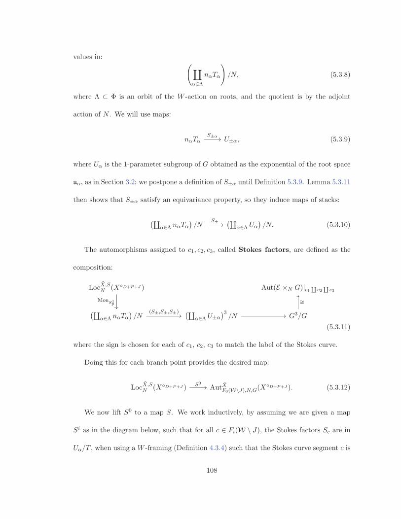
values in: (∐α∈Λ

nαTα

)/N, (5.3.8)

where Λ ⊂ Φ is an orbit of the W -action on roots, and the quotient is by the adjoint

action of N . We will use maps:

nαTα U±α,S±α

(5.3.9)

where Uα is the 1-parameter subgroup of G obtained as the exponential of the root space

uα, as in Section 3.2; we postpone a definition of S±α until Definition 5.3.9. Lemma 5.3.11

then shows that S±α satisfy an equivariance property, so they induce maps of stacks:

(∐α∈Λ nαTα

)/N

(∐α∈Λ Uα

)/N.

S±(5.3.10)

The automorphisms assigned to c1, c2, c3, called Stokes factors, are defined as the

composition:

LocX,SN (X◦D+P+J ) Aut(E ×N G)|c1 ∐ c2

∐c3

(∐α∈Λ nαTα

)/N

(∐α∈Λ U±α

)3/N G3/G

MonS1p

(S±,S±,S±)

∼=

(5.3.11)

where the sign is chosen for each of c1, c2, c3 to match the label of the Stokes curve.

Doing this for each branch point provides the desired map:

LocX,SN (X◦D+P+J ) AutXF0(W\J),N,G(X

◦D+P+J ).S0

(5.3.12)

We now lift S0 to a map S. We work inductively, by assuming we are given a map

Si as in the diagram below, such that for all c ∈ Fi(W \ J), the Stokes factors Sc are in

Uα/T , when using a W -framing (Definition 4.3.4) such that the Stokes curve segment c is

108

labelled by α. We show how to construct a map Si+1 such that the diagram commutes.

AutXFi+1(W\J),N,G(X◦D+P+J )

LocX,SN (X◦D+P+J ) AutXFi(W\J),N,G(X

◦D+P+J )

forgetSi+1

Si

(5.3.13)

The base step S0 is provided in equation 5.3.12. The inductive step of obtaining Si+1 from

Si works by picking a W -framing at the joint xi+1, and applying the N -equivariant map

from Lemma 5.3.14. This provides the Stokes factors Sc, for all Stokes curve segments c

outgoing from xi+1, and hence the lift Si+1.

Because the number of joints is finite, there is some integer N , such that FN (W) = W.

Then we define:

LocX,SN (X◦D+P+J ) AutXW,N,G(X

◦D+P+J ) AutW,G(X◦D+P+J ),

SN

S

(5.3.14)

which completes the construction.

Before proving the remaining lemmas about Stokes factors, we make some remarks

about a possible extension of Theorem 5.3.1.

Remark 5.3.7. It would be desirable to define an extended morphism nonab′ like in the

diagram below, whose restriction to LocX,SN (X◦D+P ) is nonab.

LocX,SN (X◦D+P ) LocG(X

◦D)

LocXN (X◦D+P ) LocG(X◦D+P )

nonab

nonab′

(5.3.15)

For example, this would fit well in the framework of derived symplectic geometry. Let

CD =∏

d∈D[Cd/G] denote a product of conjugacy classes of G, modulo the adjoint action

109

of G. Let LocCDG (X◦D) → LocG(X◦D) denote the substack of local systems whose mon-

odromy around each d ∈ D is constrained to be in [Cd/G]. Then we can write LocCDG (X◦D)

as a Lagrangian intersection, in the sense of [30]. This is displayed in the following di-

agram, where the horizontal arrows are evaluation of the monodromy around boundary

circles.

LocCDG (X◦D)∏

d∈D[Cd/G]×∏

p∈P [1G/G]

LocG(X◦D+P )

∏d∈D[G/G]×

∏p∈P [G/G]

(5.3.16)

Similarly, we can write LocX,SN (X◦D+P ) as a Lagrangian intersection. Then we could

interpret non-abelianization as a morphism between Lagrangian intersections. This opens

up the possibility of using the formalism of shifted symplectic structures to prove that

nonab is a symplectomorphism.

Remark 5.3.8. A naive attempt to construct nonab′ as in 5.3.15 fails, for the following

reason. We would need to extend the maps S±α from equation 5.3.9 to maps S′±α fitting

in the following diagram.

nα · T

nα · Tα U±α

S′±α

S±α

(5.3.17)

If there exists a projection T → Tα, we can obtain S′±α as a composition of S±α with

the projection nα · T → nα · Tα. However, as shown in Lemma 3.1.13, the natural map

Tα×THα → T sometimes has a kernel of order 2. In this case, the domain of definition of

S′±α cannot be nα · T , but a double cover thereof. Consequently, the domain of definition

of nonab′ must be a finite cover of LocXN (X◦D+P ). It would not be difficult to define this

finite cover and the map nonab′, but we do not carry this out.

110

5.3.1 Equivariant assignment of Stokes factors

We now state and prove some lemmas used in Construction 5.3.6.

• First, in Lemma 5.3.11, we provide an equivariant map from the monodromy of an

object of LocX,SN (X◦D+P ) to the Stokes factors used in diagram 5.3.11.

• Then, in Lemma 5.3.14, we provide an equivariant map from the Stokes factors

of incoming curves, to the Stokes factors of outgoing curves, at each joint of the

network.

Fix a branch point p. Temporarily, fix also a W -framing of the W -local system

π◦ : X◦D+R → X◦D+P at any point xp ∈ S1p (Definition 4.3.4). Under the identification

given by the framing, and due to the S-monodromy condition, the monodromy of E ∈

LocX,SN (X◦D+P ) around S1

p takes values in nα · Tα/T . (See Remark 5.2.3.)

Definition 5.3.9. Let e±α ∈ u±α be Chevalley basis elements (Definition 3.1.3). We

define the morphisms:

nα · Tα S±α−→ U±α

nαtα �−→ (u±α),

(5.3.18)

where:

u±α = Adt−1/2α

exp(−e±α). (5.3.19)

The choice of square root t1/2α is irrelevant for the adjoint action Ad

t−1/2α

.

Remark 5.3.10. Definition 5.3.9 is phrased in terms of a choice of Chevalley basis. Due

to the T -equivariance which we will prove in Lemma 5.3.11, different choices of Chevalley

111

basis actually produce the same map. However, this statement would be false if we allowed

an arbitrary basis adapted to the root space decomposition g = t⊕⊕α∈Φ gα.

Concretely, since root spaces are 1-dimensional, and since all scalar multiples of e±α

can be obtained from the adjoint action of Tα on e±α (see Lemma 3.1.15), in a new basis

we have:

e′α = adt1 eα

e′−α = adt2 e−α

for some t1, t2 ∈ Tα. Now, if we assume that adt1 = adt2 , then the relation:

nα = exp(eα) exp(e−α) exp(eα) (5.3.20)

shows that n′α = adt1(nα). Thus, T -equivariance implies that the definition of S±α using

the new basis:

Adt n′α �→ Adt exp(e

′±α) (5.3.21)

agrees with the definition of S±α.

A Chevalley basis is constrained to satisfy:

[eα, e−α] = −hα, (5.3.22)

where hα is fixed. Therefore, in two distinct Chevalley bases, it must be the case that

[eα, e−α] = [e′α, e′−α]. This forces adt1 = adt2 , justifying the assumption we had made in

the previous paragraph.

Outside the setting of Chevalley bases, there would be no reason for adt1 and adt2 to

be related, and different bases for g would give different maps in Definition 5.3.9.

112

Lemma 5.3.11. For all tα ∈ Tα, and u±α as in Definition 5.3.9, the following relation

holds in G:

nαtαuαu−αuα = id. (5.3.23)

Moreover, S±α are equivariant with respect to the adjoint action of T . As such, they

descend to morphisms of stacks:

nα · Tα/T −→ U±α/T, (5.3.24)

where the action of T is by conjugation.

Proof. In light of Lemma 3.1.14 applied to a square root t1/2α :

nαt1/2α n−1

α = t−1/2α , (5.3.25)

the relation nαtα = Adt−1/2α

nα holds. Then we can write the maps S±α in the manifestly

Tα-equivariant form:

Adt−1/2α

nα �→ Adt−1/2α

exp(−e±α). (5.3.26)

Due to Lemma 3.1.14, the adjoint action of THα on e±α and nα is trivial, so that S±α are

actually T -equivariant.

It remains to prove equation 5.3.23:

nαtαuαu−αuα =Adt−1/2α

nαAdt−1/2α

exp(−eα)Adt−1/2α

exp(−e−α)Adt−1/2α

exp(−eα)

=Adt−1/2α

(nα exp(−eα) exp(−e−α) exp(−eα)

)

=Adt−1/2α

(nαn

−1α

)=id

In the calculation above, the third equality follows from Lemma 3.1.12.

113

Next, we remove the W -framing, but work at the same branch point p. The mon-

odromy of E around S1p canonically takes values in:

(∐α∈Λ

nαTα

)/N, (5.3.27)

where Λ ⊂ Φ is a W -orbit. In this setting, we can refine Lemma 5.3.11 as follows.

Lemma 5.3.12. Let Λ denote an orbit of the W action on Φ. Let S± be the coproduct

of the maps S±α of Lemma 5.3.11, ranging over α ∈ Λ:

S± :

(∐α∈Λ

nαTα

)→∐α∈Λ

U±α. (5.3.28)

Then S± are N -equivariant, so they induce maps of stacks:

(∐α∈Λ

nαTα

)/N →

(∐α∈Λ

U±α

)/N. (5.3.29)

Proof. In light of Lemma 3.1.14, for every α ∈ Φ and tα ∈ Tα, we have nαtα = Adt−1/2α

nα,

This means that we can parametrize nαTα by Adt−1/2α

nα, where tα ranges over Tα. More-

over, we can parametrize∐

α nαTα by Adn nα, where α is fixed and n ranges over N .

Let [n] denote the image of n under the projection to W , and α′ = [n](α). Then,

according to Lemma 3.1.16, there exists t0 ∈ Tα′ such that:

• adn0(e±α) = adt0(e±α′);

• Adn0(nα) = Adt0(nα′).

Then S±(Adn nα) is the following composition, which is manifestly N -equivariant.

Adn nα Adn exp(−eα)

Adt0(nα′) Adt0 exp(−eα′)

Lem. 3.1.16

Eq. 5.3.26

Lem. 3.1.16 (5.3.30)

114

We move on to the equivariant map between incoming and outgoing Stokes factors at

a joint x of W. Temporarily fix a trivialization φx : Ex ∼= N of the fiber of the N -local

system over the joint. Then φx determines aW -framing at x, which determines a labeling

of the Stokes curves segments incident to x by roots (see Remark 4.3.5). Moreover, φx

determines an isomorphism:

Aut(E ×N G)|x ∼= G. (5.3.31)

Due to the inductive procedure in Construction 5.3.6, we assume that we already have

Stokes factors for the incoming Stokes curves at x; furthermore, we can assume that, for

an incoming curve labeled by γ ∈ Φ, the image of the Stokes factor under 5.3.31 is an

element uγ ∈ Uγ . This discussion, together with the convexity result in 4.1.20, proves:

Lemma 5.3.13. Under a trivialization φx : Ex ∼= N , the structure of the spectral network

in the neighborhood of the joint x is locally modeled by an undecorated 2D scattering

diagram.

According to Theorem 3.2.21, the scattering diagram has a unique solution, i.e. there

is a unique morphism of schemes:

∏γ∈Cin

Uγ −→∏

γ∈Cout

Uγ

(uγ)γ∈Cin �−→ (u′γ)γ∈Cout

(5.3.32)

such that the product uCout (equation 3.2.36) is the identity in G. We interpret the

relation uCout = id as saying that the re-glued local system has no monodromy around

the joint x.

Then, we define the outgoing Stokes factors as the preimages of (u′γ)γ∈Cout , under the

identification 5.3.31 determined by the trivialization φx. It remains to show that this

115

definition does not depend on φx. This follows from the next lemma.

Lemma 5.3.14. Let Λ be an orbit of the action ofW on convex, ordered subsets of Φ. For

every Cin ∈ Λ, define Cout := ConvNCin. Consider the coproduct, ranging over Cin ∈ Λ, of

the morphisms given by Theorem 3.2.21:

∐Cin∈Λ

∏γ∈Cin

Uγ −→∐

Cin∈Λ

∏γ∈Cout

Uγ . (5.3.33)

It is N -equivariant with respect to the adjoint action of N , acting diagonally on the factors

of the product, but permuting factors of the coproduct. As a consequence, it descends to

a morphism of stacks:⎛⎝ ∐

Cin∈Λ

∏γ∈Cin

Uγ

⎞⎠ /N →

⎛⎝ ∐

Cin∈Λ

∏γ∈Cout

Uγ

⎞⎠ /N. (5.3.34)

Proof. For every Cin ∈ Λ, Theorem 3.2.21 asserts that there is a unique tuple (u′γ)γ∈Cout ,

such that the product uCout from equation 3.2.36 is the identity. This takes the explicit

form

−→∏γ∈Cin

∐Cout

u±1γ = id, (5.3.35)

where the product is ordered clockwise around the joint, and the exponent is −1 for

incoming curves and +1 for outgoing curves. Applying Adn to this equation, and using

the uniqueness of the solution, the result follows.

116

Bibliography

[1] Takashi Aoki, Takahiro Kawai, and Yoshitsugu Takei, On the exact steepest descent

method: a new method for the description of Stokes curves, Journal of Mathematical

Physics 42 (2001), no. 8, 3691–3713.

[2] David Aulicino, The Cantor-Bendixson rank of certain Bridgeland-Smith stability

conditions, Communications in Mathematical Physics (2015).

[3] Arnaud Beauville, MS a Narasimhan, and S Ramanan, Spectral curves and the gen-

eralised theta divisor, J. reine angew. Math 398 (1989), 169–179.

[4] H. L. Berk, William McCay Nevins, and K. V. Roberts, New Stokes’ line in WKB

theory, Journal of Mathematical Physics 23 (1982), no. 6, 988–1002.

[5] Philip Boalch, Quasi-hamiltonian geometry of meromorphic connections, Duke Math.

J. 139 (2007), no. 2, 369–405.

[6] Nicolas Bourbaki, Lie groups and Lie algebras, Part I: Chapters 1-3, Hermann,

Addison-Wesley, 1975.

[7] Tom Bridgeland and Valerio Toledano Laredo, Stability conditions and Stokes factors,

Inventiones mathematicae 187 (2012), no. 1, 61–98.

117

[8] Tom Bridgeland and Ivan Smith, Quadratic differentials as stability conditions, Pub-

lications mathematiques de l’IHES 121 (2015), no. 1, 155–278.

[9] C. Chevalley, Sur certains groupes simples, Tohoku Math. J. (2) 7 (1955), no. 1-2,

14–66.

[10] Ron Donagi, Decomposition of spectral covers, In Current topics in complex algebraic

geometry, Citeseer, 1993.

[11] , Spectral covers, Current Topics in Complex Algebraic Geometry (Berkeley,

CA 1992/93), Math. Sci. Res. Inst. Publ 28 (1995), 65–86.

[12] Ron Donagi and Dennis Gaitsgory, The gerbe of Higgs bundles, Transformation

groups 7 (2002), no. 2, 109–153.

[13] Gerd Faltings, Stable G-bundles and projective connections, J. Algebraic Geom 2

(1993), no. 3, 507–568.

[14] Aaron Fenyes, Abelianization of SL(2,R) local systems, arXiv preprint

arXiv:1510.05757 (2015).

[15] Vladimir Fock and Alexander Goncharov, Moduli spaces of local systems and higher

Teichmuller theory, Publications Mathematiques de l’Institut des Hautes Etudes

Scientifiques 103 (2006), no. 1, 1–211.

[16] Davide Gaiotto, Gregory W Moore, and Andrew Neitzke, Spectral networks, Annales

Henri Poincare, vol. 14, Springer, 2013, pp. 1643–1731.

118

[17] , Wall-crossing, Hitchin systems, and the WKB approximation, Advances in

Mathematics 234 (2013), 239–403.

[18] , Spectral networks and snakes, Annales Henri Poincare, vol. 15, Springer,

2014, pp. 61–141.

[19] Nigel J Hitchin, The self-duality equations on a Riemann surface, Proceedings of the

London Mathematical Society 3 (1987), no. 1, 59–126.

[20] Nigel J. Hitchin, Stable bundles and integrable systems, Duke mathematical journal

54 (1987), no. 1, 91–114.

[21] Lotte Hollands and Andrew Neitzke, Spectral networks and Fenchel–Nielsen coordi-

nates, Letters in Mathematical Physics 106 (2016), no. 6, 811–877.

[22] Naofumi Honda, Takahiro Kawai, and Yoshitsugu Takei, Virtual turning points,

Springer, 2015.

[23] Matei Ionita and Benedict Morrissey, Spectral networks and non-abelianization, to

appear.

[24] Kohei Iwaki and Tomoki Nakanishi, Exact WKB analysis and cluster algebras, Jour-

nal of Physics A: Mathematical and Theoretical 47 (2014), no. 47, 474009.

[25] , Exact WKB analysis and cluster algebras II: Simple poles, orbifold points,

and generalized cluster algebras, International Mathematics Research Notices 2016

(2015), no. 14, 4375–4417.

119

[26] Alexander Kirillov, Jr., An introduction to Lie groups and Lie algebras, Cambridge

Studies in Advanced Mathematics, vol. 113, Cambridge University Press, Cambridge,

2008. MR 2440737

[27] Pietro Longhi and Chan Y Park, ADE spectral networks, Journal of High Energy

Physics 2016 (2016), no. 8, 87.

[28] Bao Chau Ngo, Le lemme fondamental pour les algebres de Lie, Publications

mathematiques de l’IHES 111 (2010), no. 1, 1–169.

[29] Nikita Nikolaev, Abelianisation of Logarithmic sl2-connections, arXiv preprint alg-

geom/1902.03384 (2019).

[30] Tony Pantev, Bertrand Toen, Michel Vaquie, and Gabriele Vezzosi, Shifted symplectic

structures, Publications mathematiques de l’IHES 117 (2011).

[31] Renata Scognamillo, An elememtary approach to the abelianization of the Hitchin

system for arbitrary reductive groups, Compositio Mathematica 110 (1998), no. 1,

17–37.

[32] Carlos Simpson, The Hodge filtration on nonabelian cohomology, arXiv preprint alg-

geom/9604005 (1996).

[33] Carlos T Simpson, Nonabelian Hodge theory, Proceedings of the International

Congress of Mathematicians, vol. 1, 1990, pp. 747–756.

[34] , Higgs bundles and local systems, Publications Mathematiques de l’Institut

des Hautes Etudes Scientifiques 75 (1992), no. 1, 5–95.

120

[35] K Strebel, Quadratic differentials, vol. 5, Springer Science & Business Media, 1984.

[36] Yoshitsugu Takei, WKB analysis and Stokes geometry of differential equations, An-

alytic, algebraic and geometric aspects of differential equations, Springer, 2017,

pp. 263–304.

[37] Terrence Tao, Notes on the classification of complex Lie alge-

bras, Blog post https://terrytao.wordpress.com/2013/04/27/

notes-on-the-classification-of-complex-lie-algebras/, 2018 version.

121