MAT 254 – Probability and Statistics Sections 1,2 & 3 2015 ...D0004...Tabulated t (df7), with level of significance 0.05, two tails, = 2.36 We reject Ho and conclude that there is

4/29/2015

1

MAT 254 – Probability and StatisticsSections 1,2 & 3

2015 - Spring

1) Importance and basic concepts of Probability and Statistics. Introduction to Statistics and data analysis

2) Data collection and presentation3) Measures of central tendency; mean, median, mode4) Probability5) Conditional probability 6) Discrete probability distributions7) Continuous probability distributions

Midterm Exam (April 1, 17:30)8) Hypothesis testing (2 weeks)9) Student t-test (2 weeks)10) Chi-square11) Correlation and regression analysis12) REVIEW

Final Exam (May 25- June 7)

web.adu.edu.tr/user/oboyaci

MAT254 - Probability & Statistics 2

4/29/2015

2

MAT254 - Probability & Statistics

One sample t‐test

dependent samples(Paired)

Independent samples(Unpaired)

3

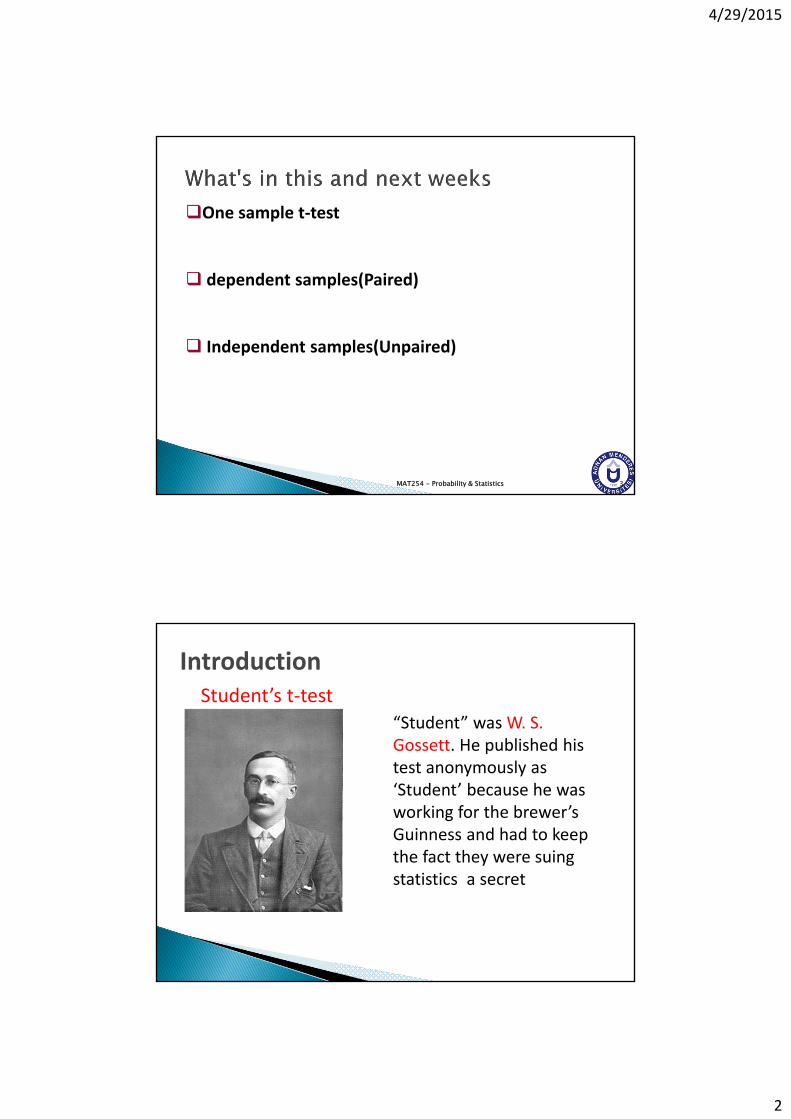
Student’s t‐test“Student” was W. S. Gossett. He published his test anonymously as ‘Student’ because he was working for the brewer’s Guinness and had to keep the fact they were suing statistics a secret

Introduction

4/29/2015

3

Student’s t‐test

The test is used to compare samples from two different batches.

It is usually used with small (<30) samples that are normally distributed.

The t‐test is a basic test that is limited to two groups. For multiple groups, you would have to compare each pair of groups, for example with three groups there would be three tests (AB, AC, BC), whilst with seven groups there would need to be 21 tests.

The basic principle is to test the null hypothesis that the means of the two groups are equal.

The t‐test assumes: ◦ A normal distribution (parametric data)◦ Underlying variances are equal (if not, use Welch's test)

It is used when there is random assignment and only two sets of measurement to compare.

4/29/2015

4

Single sample t – we have only 1 group; want to test against ahypothetical mean.

Independent samples t – we have 2 means, 2 groups; no relation between groups, e.g., people randomly assigned to a single group.

Dependent t – we have two means. Either same people in both groups,or people are related, e.g., husband‐wife, left hand‐right hand, hospital and visitor.

MAT254 ‐ Probability & Statistics 7

The t distribution is a short, fat relative of the normal. The shape of t depends on its df. As N becomes infinitely large, t becomes normal.


4/29/2015

5

9

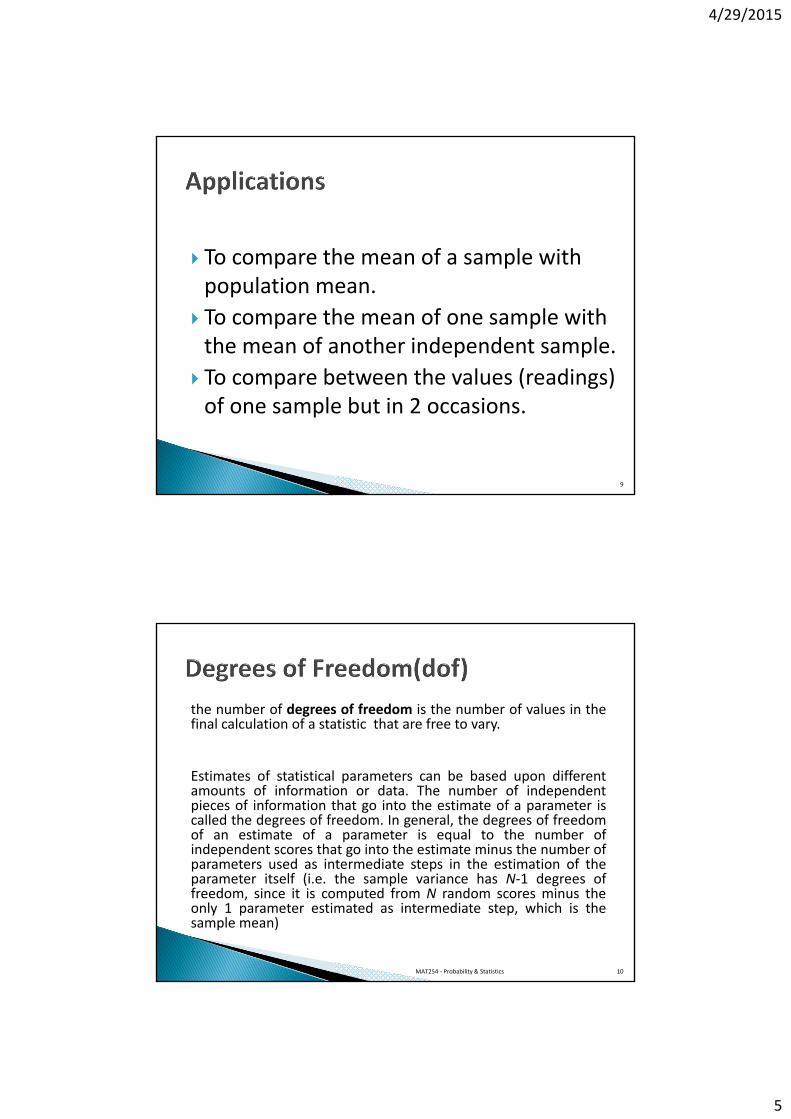
To compare the mean of a sample with population mean.

To compare the mean of one sample with the mean of another independent sample.

To compare between the values (readings) of one sample but in 2 occasions.

the number of degrees of freedom is the number of values in thefinal calculation of a statistic that are free to vary.

Estimates of statistical parameters can be based upon differentamounts of information or data. The number of independentpieces of information that go into the estimate of a parameter iscalled the degrees of freedom. In general, the degrees of freedomof an estimate of a parameter is equal to the number ofindependent scores that go into the estimate minus the number ofparameters used as intermediate steps in the estimation of theparameter itself (i.e. the sample variance has N‐1 degrees offreedom, since it is computed from N random scores minus theonly 1 parameter estimated as intermediate step, which is thesample mean)

MAT254 ‐ Probability & Statistics 10

4/29/2015

6

11

It is used in measuring whether a sample valuesignificantly differs from a hypothesized value.For example, a research scholar might hypothesize thaton an average it takes 3 minutes for people to drink astandard cup of coffee. He conducts an experiment andmeasures how long it takes his subjects to drink astandard cup of coffee. The one sample t‐test measureswhether the mean amount of time it took theexperimental group to complete the task variessignificantly from the hypothesized 3 minutes value.

12

It is used in comparing the means of two variablesfor a single group. This test computes thedifferences between values of two variables foreach case and tests whether the average differsfrom 0. For example, in a study on impact of aparticular diet on weight, all patients aremeasured at the beginning of the study, prescribeda fixed diet, and measured again. Thus eachsubject has two measures, often called before andafter measures.

4/29/2015

7

13

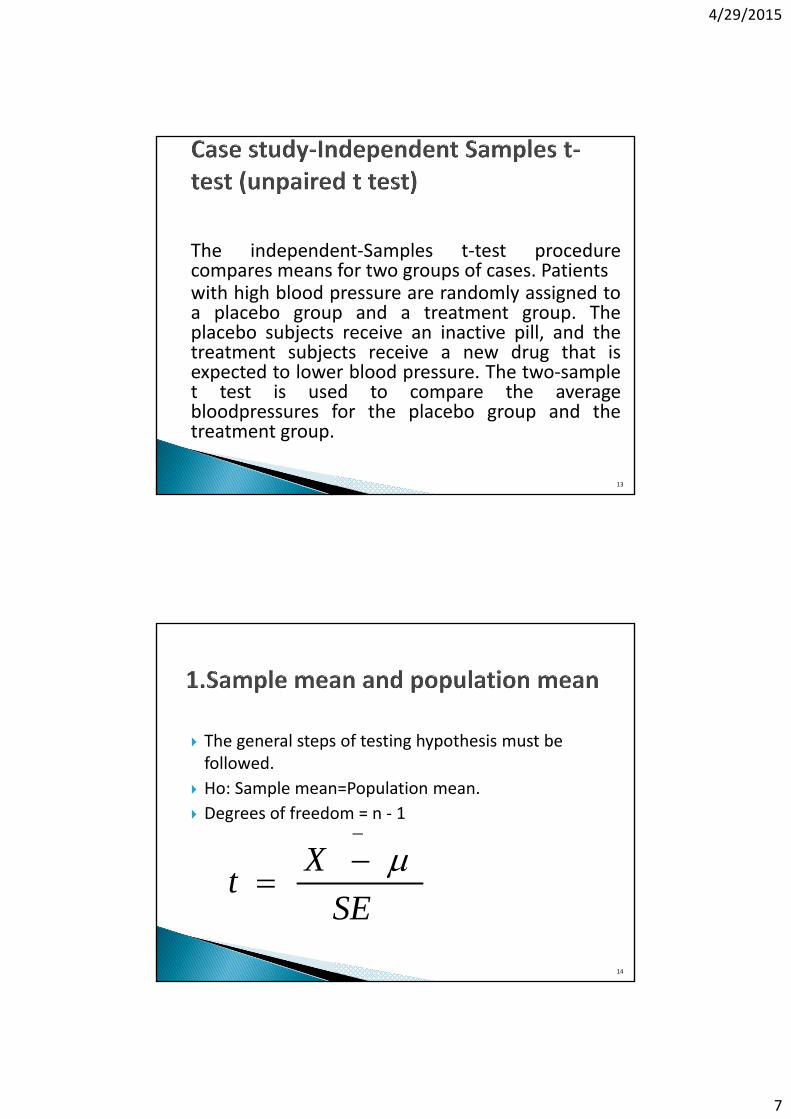
The independent‐Samples t‐test procedurecompares means for two groups of cases. Patientswith high blood pressure are randomly assigned toa placebo group and a treatment group. Theplacebo subjects receive an inactive pill, and thetreatment subjects receive a new drug that isexpected to lower blood pressure. The two‐samplet test is used to compare the averagebloodpressures for the placebo group and thetreatment group.

14

The general steps of testing hypothesis must be followed.

Ho: Sample mean=Population mean.

Degrees of freedom = n ‐ 1

SE

Xt

4/29/2015

8

15

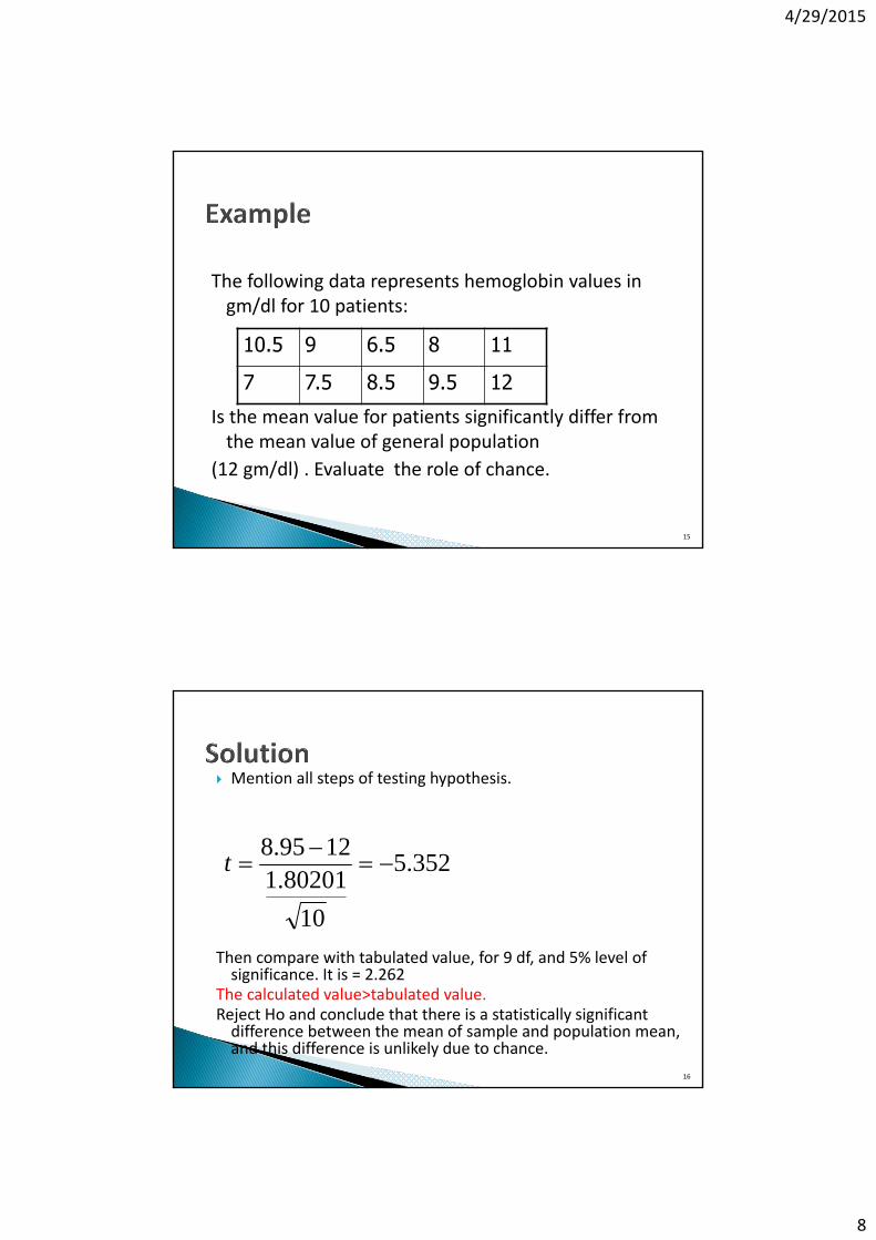
The following data represents hemoglobin values in gm/dl for 10 patients:

Is the mean value for patients significantly differ from the mean value of general population

(12 gm/dl) . Evaluate the role of chance.

10.5 9 6.5 8 11

7 7.5 8.5 9.5 12

16

Mention all steps of testing hypothesis.

Then compare with tabulated value, for 9 df, and 5% level of significance. It is = 2.262

The calculated value>tabulated value.Reject Ho and conclude that there is a statistically significant difference between the mean of sample and population mean, and this difference is unlikely due to chance.

352.5

10

80201.11295.8

t

4/29/2015

9

17

18

When have two dependent or related samples. • Same group measured twice (Time 1 vs. Time 2; Pretest and Posttest).

• Samples are matched on some variable. Each score in one sample is paired with a specific score in the other sample.

Such data are correlated data.

4/29/2015

10

19

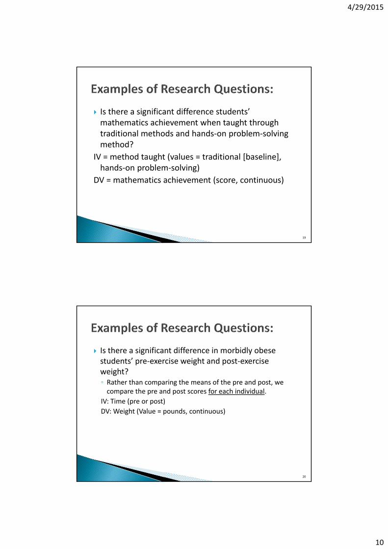
Is there a significant difference students’ mathematics achievement when taught through traditional methods and hands‐on problem‐solving method?

IV = method taught (values = traditional [baseline], hands‐on problem‐solving)

DV = mathematics achievement (score, continuous)

20

Is there a significant difference in morbidly obese students’ pre‐exercise weight and post‐exercise weight? ◦ Rather than comparing the means of the pre and post, we compare the pre and post scores for each individual.

IV: Time (pre or post)

DV: Weight (Value = pounds, continuous)

4/29/2015

11

21

Null hypothesis:or Ho: µD ≥ 0 or Ho: µD ≤ 0

Alternative hypothesis:

or or

* Subscript D indicates difference.

01: H D01: H D

01: H D

00: H D

22

1) Compute degrees of freedom

df = n – 1 whereby n = number of pairs

2) Set alpha level

3) Locate critical value(s)

4/29/2015

12

23

Whereby:

D =

after‐before

= Sample Standard Deviation of difference (D) scores, divided

by

S D

Dt

xx 12

SD

n

S D

n

DD

Sum of individual differences

24

Before After D = after ‐ before

5 6 1

8 9 1

4 5 1

3 6 3

7 7 0

8 10 2

S D

Dt

8203111D

42.6

03.1

nSS D

D

09.342.

3.1

S D

Dt

3.16

8

n

DD Standard

deviation of the differences

Number of pairs

4/29/2015

13

25

Use t distribution in the appendix to find the critical values (given alpha level, df, and directionality of the test).

In this example,

df = n‐1= 6‐1 = 5

26

Use t distribution in the to find the critical values (given alpha level, df, and directionality of the test).

The graph on the right shows an example of two‐tailed test with the c.v. equal to ± 2.776.

With alpha = 0.05 and df = 5, the critical values are ± 2.571 (two‐tailed test).

Conclusion: Reject H0

4/29/2015

14

27

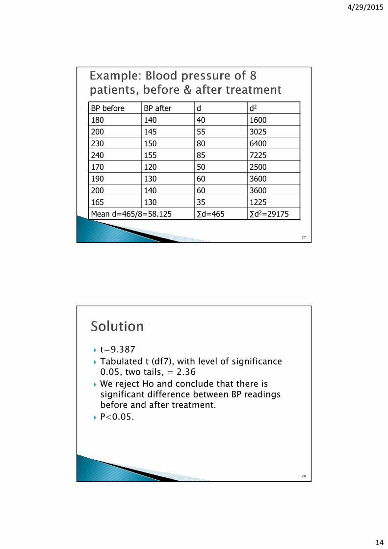
BP before BP after d d2

180 140 40 1600200 145 55 3025230 150 80 6400240 155 85 7225170 120 50 2500190 130 60 3600200 140 60 3600165 130 35 1225Mean d=465/8=58.125 ∑d=465 ∑d2=29175

28

t=9.387 Tabulated t (df7), with level of significance

0.05, two tails, = 2.36 We reject Ho and conclude that there is

significant difference between BP readings before and after treatment.

P<0.05.

4/29/2015

15

29

The reason for hypothesis testing is to gain knowledge about an unknown population.

Independent samples t‐test is applied when we have two independent samples and want to make a comparison between two groups of individuals. The parameters are unknown.

How is this different than a Z‐test and One Sample t‐test?

30

We are interested in the difference between two independent groups. As such, we are comparing two populations by evaluating the mean difference.

In order to evaluate the mean difference between two populations, we sample from each population and compare the sample means on a given variable.

Must have two independent groups (i.e.samples) and one dependent variable that is continuous to compare them on.

4/29/2015

16

31

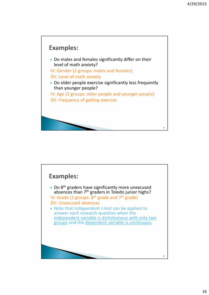
Do males and females significantly differ on their level of math anxiety?

IV: Gender (2 groups: males and females)DV: Level of math anxiety Do older people exercise significantly less frequently than younger people?

IV: Age (2 groups: older people and younger people)DV: Frequency of getting exercise

32

Do 8th graders have significantly more unexcused absences than 7th graders in Toledo junior highs?

IV: Grade (2 groups: 8th grade and 7th grade)DV: Unexcused absences Note that Independent t‐test can be applied to answer each research question when the independent variable is dichotomous with only two groups and the dependent variable is continuous.

4/29/2015

17

33

Ho: The null hypothesis states that the two samples come from the same population. In other words, There is no statistically significant difference between the two groups on the dependent variable.

Symbols:Non-directional: Ho: μ1 = μ2

Directional: or

• If the null hypothesis is tenable, the two group means differ only by sampling fluctuation – how much the statistic’s value varies from sample to sample or chance.

21

:0 H21

:0 H

34

Ha: The alternative hypothesis states that the two samples come from different populations. In other words, There is a statistically significant difference between the two groups on the dependent variable.

Symbols:Non-directional:

Directional:

21

:1 H

21

:1 H

21

:1 H

4/29/2015

18

35

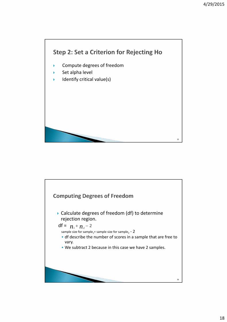
Compute degrees of freedom

Set alpha level

Identify critical value(s)

36

Calculate degrees of freedom (df) to determine rejection region.df = sample size for sample1+ sample size for sample2 ‐ 2• df describe the number of scores in a sample that are free to vary.

• We subtract 2 because in this case we have 2 samples.

221 nn

4/29/2015

19

37

• In an Independent samples t-test, each sample mean places a restriction on the value of one score in the sample, hence the sample lost one degree of freedom and there are n-1 degrees of freedom for the sample.

38

Set at .001, .01 , .05, or .10, etc.

4/29/2015

20

39

nnnnnsnsxxt

2121

2

2

21

2

1

21

112

11

Whereby:n: Sample size s2 = variance

:Sample mean subscript1 = sample 1 or group 1

subscript2 = sample 2 or group 2

x

df

variance

40

df = 18 α = .05 , two‐tailed test in this example• critical values are ± 2.101 in this example

4/29/2015

21

41

Fail to reject the null hypothesis and conclude that there is no statistically significant difference between the two groups on the dependent variable, t = , p > α.

OR

Reject the null hypothesis and conclude that there is a statistically significant difference between the two groups on the dependent variable, t = , p < α.

• If directional, indicate which group is higher or lower (greater, or less than, etc.).

42

Variable Math anxiety tGender

Male 3.66Female 3.98 3.35***

AgeUnder 40 years 3.32Over 41 years 3.64 2.67**

Note. **p < .01. ***p < .001.

4/29/2015

22

43

The following data represents weight in Kg for 10 males and 12 females.

Males:

Females:

80 75 95 55 60

70 75 72 80 65

60 70 50 85 45 60

80 65 70 62 77 82

44

Is there a statistically significant difference between the mean weight of males and females. Let alpha = 0.01

To solve it follow the steps and use this equation.

)11

(2

)1()1(

2121

222

211

21

nnnnSnSn

XXt

4/29/2015

23

45

Mean1=72.7 Mean2=67.17 Variance1=128.46 Variance2=157.787 df = n1+n2‐2=20 t = 1.074 The tabulated t, 2 sides, for alpha 0.01 is 2.845 Then, fail to reject Ho and conclude that there is no significant difference between the 2 means. This difference may be due to chance.

P>0.01

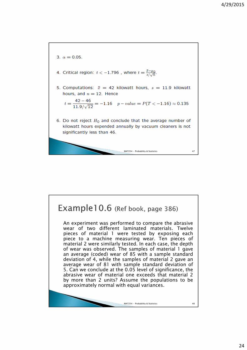
The Edison Electric Institute has published figures on thenumber of kilowatt hours used annually by various homeappliances. It is claimed that a vacuum cleaner uses anaverage of 46 kilowatt hours per year. If a random sample of12 homes included in a planned study indicates that vacuumcleaners use an average of 42 kilowatt hours per year with astandard deviation of 11.9 kilowatt hours, does this suggest atthe 0.05 level of significance that vacuum cleaners expend, onthe average, less than 46 kilowatt hours annually? Assumethe population of kilowatt hours to be normal.


4/29/2015

24


An experiment was performed to compare the abrasivewear of two different laminated materials. Twelvepieces of material 1 were tested by exposing eachpiece to a machine measuring wear. Ten pieces ofmaterial 2 were similarly tested. In each case, the depthof wear was observed. The samples of material 1 gavean average (coded) wear of 85 with a sample standarddeviation of 4, while the samples of material 2 gave anaverage wear of 81 with sample standard deviation of5. Can we conclude at the 0.05 level of significance, theabrasive wear of material one exceeds that material 2by more than 2 units? Assume the populations to beapproximately normal with equal variances.


4/29/2015

25


Decision and conclusion: Do not reject H0. We are unable to conclude that the abrasive wear of material 1 exceeds that of material 2 by more than 2 units.


4/29/2015

26

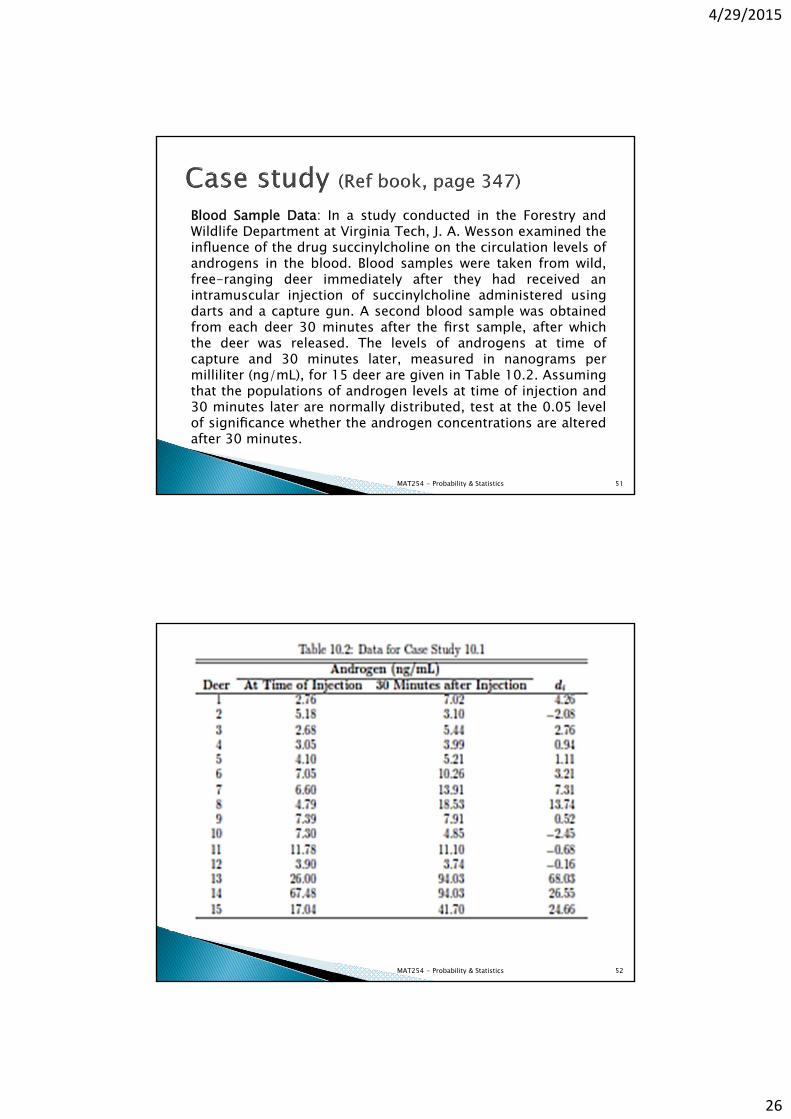
Blood Sample Data: In a study conducted in the Forestry andWildlife Department at Virginia Tech, J. A. Wesson examined theinfluence of the drug succinylcholine on the circulation levels ofandrogens in the blood. Blood samples were taken from wild,free-ranging deer immediately after they had received anintramuscular injection of succinylcholine administered usingdarts and a capture gun. A second blood sample was obtainedfrom each deer 30 minutes after the first sample, after whichthe deer was released. The levels of androgens at time ofcapture and 30 minutes later, measured in nanograms permilliliter (ng/mL), for 15 deer are given in Table 10.2. Assumingthat the populations of androgen levels at time of injection and30 minutes later are normally distributed, test at the 0.05 levelof significance whether the androgen concentrations are alteredafter 30 minutes.



4/29/2015

27


To find out whether a new serum will arrestleukemia, 9 mice, all with an advanced stage of thedisease, are selected. Five mice receive thetreatment and 4 do not. Survival times, in years,from the time the experiment commenced are asfollows:Treatment 2.1 5.3 1.4 4.6 0.9No Treatment 1.9 0.5 2.8 3.1At the 0.05 level of significance, can the serum besaid to be effective? Assume the two populations tobe normally distributed with equal variances.


4/29/2015

28

The hypotheses areH0: µ1-µ2=0H1:µ1-µ2<0α=0.05Critical region :t>ttabulated=1.895 with 7 degrees of freedom (from appendix table, A.4)Computation:

ttabulated is higher than tcalculated wecan not reject H0.


69.0

)11

(2

)1()1(

2121

222

211

21

nnnnSnSn

XXt

End of lecture…


Documents

MAT 254 – Probability and Statistics Sections 1,2 & 3 2015 ...D0004...Tabulated t (df7), with level of significance 0.05, two tails, = 2.36 We reject Ho and conclude that there is