Embed Size (px)
Citation preview

Master’s Thesis
A Comparative Simulation Study of Chemical EOR Methodologies (Alkaline, Surfactant and/or Polymer) Applied to Norne Field E-Segment August, 2011
Yugal Kishore Maheshwari
Supervisor: Professor Jon Kleppe
Department of Petroleum Engineering and Applied Geophysics

Faculty of Engineering and Technology Department of Petroleum Engineering and Applied Geophysics
Master’s Thesis
by
Yugal Kishore Maheshwari
Thesis started: March 20, 2011
Thesis submitted: August 16, 2011
Study program: MSc. Petroleum Engineering
Specialization: Reservoir Engineering
Title of Thesis: A Comparative Simulation Study of Chemical EOR Methodologies (Alkaline, Surfactant and/or Polymer) Applied to Norne Field E-Segment
This work has been carried out at the Department of Petroleum Engineering and Applied Geophysics, under the supervision of Professor Jon Kleppe
Trondheim, August 16, 2011
Jon Kleppe
Supervisor
Professor and Head of Department

ii
Abstract
Abstract
Primary and Secondary Recovery techniques together are able to recover only
about 35-50% of oil from the reservoir. This leaves a significant amount of oil
remaining in the reservoir. The residual oil left after the water flooding is either
from water swept part or area by-passed by the water flooding. The by-passed
residual oil has a high interfacial tension with the water. One way of recovering
this capillary trapped oil is by flooding the reservoir with chemicals (surfactant,
alkali-surfactant (AS), surfactant-polymer (SP), or alkaline-surfactant-polymer
(ASP)).
The Norne field which is the base case for this study having approximately
current recovery factor of 60% with water flooding is one of the best subsea
fields in the world. The oil production has peaked in 2001 and is now declining.
The pockets of residual oil saturation are still trapped in the reservoir especially
in the Ile and Tofte formations. The water flooding alone cannot recover capillary
trapped oil pockets efficiently, thus requires enhanced oil recovery techniques.
The EOR screening criteria suggested by Taber et al. (1) was applied to Norne E-
segment in order to come up with the right EOR method that would reduce
residual oil saturation to the minimum. Five EOR scenarios such as surfactant
flooding, alkaline-surfactant flooding, polymer flooding, surfactant-polymer
flooding, and alkaline-surfactant-polymer flooding were simulated for the Norne
E-segment.
The main objective of this study was to do a comparative simulation study to
evaluate the effectiveness of these chemical methods (scenarios) compared to a
conventional waterflooding in terms of incremental oil production. After this,
one of the flooding methods was to be concluded for the Norne E-segment based
on incremental net present value (NPV).
The injection well F-3H and producer E-2H were evaluated as the most promising
wells for above scenarios. A series of cases were run to ascertain the injection
length, appropriate surfactant quantity and concentration. Five scenarios with
different combination and concentrations of chemicals (alkali, surfactant and
polymer) were run using Eclipse 100. In addition, calculation of incremental NPV
based on incremental oil production for all scenarios; single parameter sensitivity
analysis (Spider plot) for low case, base case, and high case at different oil prices,
chemicals prices, and discount rate were also performed. It was found that

iii
Abstract
change in oil price has substantial effect on NPV compared to other parameters
while surfactant price is the least sensitive parameter i.e very low affect on NPV
for high/low case.
From simulation results and economics analysis, ASP flooding was found to be
better than other chemical methods (scenarios) in terms of incremental NPV for
the Norne E-segment. However, the 1.40 % incremental recovery factor by ASP
flooding seems not so high and will have an incremental net present value of
+123.53 million USD. It is noted that the additional costs regarding operations
and installations were not included in the economics calculation. The recovery
factor as well as NPV can be optimized with accurate chemical designing in
laboratory and modeling of compositional model in Chemical Compositional
Simulator. It is recommended that right alkali, surfactant and polymer structure
that would be compatible with fluid and rock properties of Norne field E-
segment, be developed in the laboratory. It is also important that up-scaling the
appropriate laboratory identified chemicals to a field-scale usage be done
correctly. The timing of ASP injection into Norne E-segment is also recommended
to be early in the life of the field because injection of ASP at a later time might
not lead to best possible oil recovery.

iv
Dedication
Dedication
My great thanks go to my respected parents, my in-laws, my siblings, my sweet
wife Hemlata Maheshwari, my two lovely kids Yash Kishore Maheshwari, Muskan
Maheshwari and cute nieces Jiya and Harsha for their prayers, patience and
support during my master program. I am sorry that I could not spend time with
you during my studies.
My sincere gratitude goes to Mr. Muhammad Mureed Rahimoon, my father-in-
law Mr. Abheman Ladher and, my relatives Mr. Ashok Kumar Ranjhani and Mr.
Chaman Lal for their cooperation.

v
Acknowledgements
Acknowledgements
I would like to express my deep gratitude to my supervisor Professor Jon Kleppe,
Head of Department and Richard Rwechungura, PhD Scholar for their continuous
help, encouragement and advice during the thesis period. Great thanks to Dr.
Lars Høier (Statoil), Nan Cheng (Statoil), specialist Jan Åge Stensen (SINTEF),
Charles A. Kossak (Schlumberger), and Kippe Vegard (Statoil). I thank you all for
providing me with alkaline/surfactant/polymer properties and advises through
email. I feel the need to thank my friends Arindam Arang, Chinenye Clara and
Samson Imoh Essien for their suggestions and ideas.
I also wish to say a big thank you to the Center of Integrated Operations at
NTNU, Statoil ASA and its license partners ENI and Petoro for the release of
Norne data.
Finally, I wish to give my sincere thanks to Lånekassen (QUOTA Scheme) and
department of Petroleum Engineering and Applied Geophysics for providing me
financial support to pursue my graduate studies.
Trondheim, August 2011
Yugal Kishore Maheshwari [email protected]

vi
Nomenclature
Nomenclature
ɸ porosity
interfacial tension between the displaced and the displacing fluids
mass density of the rock formation
Mobility
Todd-Longstaff mixing parameter
adsorption multiplier at alkaline concentration
alkaline concentrations
alkaline adsorption concentration
surfactant/polymer adsorbed concentration
polymer adsorption concentration
polymer and salt concentrations respectively in the aqueous
phase
cell center depth
water production rate
relative permeability reduction factor for the aqueous phase due
to polymer retention
dead pore space within each grid cell
transmissibility
displaced fluid viscosity
shear viscosity of the polymer solution (water + polymer)
effective water viscosity
µs Surfactant viscosity
µws Water-surfactant solution viscosity
µw Water viscosity
effective viscosity of salt
effective viscosity of the water (a=w), polymer (a=p) and salt (a=s).
pore velocity

vii
Nomenclature
block pore volume
ASP Alkaline, surfactant and polymer
AS Alkaline and surfactant
AP Alkaline and polymer
CDC Capillary Desaturation Curve
CMC Critical Micelle Concentration
Cunit A unit constant
CA(Csurf ) Adsorption as a function of local surfactant concentration
EOR Enhanced Oil Recovery
IEA International Energy Agency
IFT Interfacial Tension
K Permeability
MD Mass Density
Nc Capillary Number
NPD Norwegian Petroleum Directory
NPV Net Present Value
P Potential
Pcow Capillary pressure
Pcow(Sw) Capillary pressure from the initially immiscible curve scaled
according to the end points
Pref Reference pressure
PORV Pore volume in a cell
Sorw Residual oil saturation after water flooding
ST Interfacial tension
ST(Csurf) Surface tension with present surfactant concentration
ST(Csurf = 0) Surface tension with no surfactant present
viii
<Table of Contents
Table of Contents
Abstract ................................................................................................................................ ii
Dedication ........................................................................................................................... iv
Acknowledgements.............................................................................................................. v
Nomenclature ..................................................................................................................... vi
Table of Contents .............................................................................................................. viii
List of Figures ..................................................................................................................... xii
List of Tables ..................................................................................................................... xiv
1 Introduction ............................................................................................................... 1
1.1 Objective ............................................................................................................. 3
1.2 Enhanced Oil Recovery ....................................................................................... 5
1.3 Classification of EOR Processes ........................................................................... 5
1.4 Principles of Enhanced Oil Recovery (EOR)......................................................... 7
1.4.1 Improving the Mobility Ratio ...................................................................... 7
1.4.2 Increasing the Capillary Number ................................................................. 8
2 Norne Field ................................................................................................................. 9
2.1 General Field Information ................................................................................... 9
2.2 Development..................................................................................................... 10
2.3 Geology of the Norne Field ............................................................................... 11
2.3.1 Stratigraphy and Sedimentology .............................................................. 11
2.4 Reservoir Communication................................................................................. 13
2.4.1 Faults ......................................................................................................... 13
2.4.2 Stratigraphic barriers ................................................................................ 13
2.5 Drainage Strategy.............................................................................................. 14
3 Norne Field E-Segment ............................................................................................. 16
3.1 The Reservoir Simulation Model ....................................................................... 16
3.2 EOR Potential in Norne E-segment ................................................................... 18
3.3 EOR Screening Criteria of the Norne E-Segment .............................................. 20
4 Overview of Surfactant, Alkaline and Polymer Flooding ......................................... 22
4.1 Surfactant Flooding ........................................................................................... 22

ix
<Table of Contents
4.1.1 Basic Surfactant Classification .................................................................. 22
4.1.2 Methods to Characterize Surfactants ....................................................... 23
4.1.3 Surfactant Flooding in Petroleum Reservoirs ........................................... 25
4.2 Polymer Flooding .............................................................................................. 31
4.2.1 Types of Polymers ..................................................................................... 31
4.2.2 Polymer Flow Behavior in Porous Media .................................................. 34
4.3 Alkaline Flooding ............................................................................................... 36
4.3.1 Alkaline Reaction with Crude Oil............................................................... 37
4.4 Alkaline Surfactant Polymer (ASP) Flooding ..................................................... 39
5 Simulation of Alkaline, Surfactant and Polymer Flooding ........................................ 41
5.1 The Surfactant Flood Model ............................................................................. 41
5.2 The Polymer Flood Model ................................................................................. 41
5.3 The Alkaline Flood Model ................................................................................. 41
5.4 Alkaline, Surfactant and Polymer Properties .................................................... 42
5.5 Performance and Economic Evaluation ............................................................ 42
5.6 Synthetic Model for Testing of Alkaline, Surfactant and Polymer Flooding
Models .......................................................................................................................... 43
5.7 Overview of Base Case ...................................................................................... 46
5.8 Selection of Injector and Producer ................................................................... 46
5.9 Assumptions ...................................................................................................... 48
6 Simulation Results and Analysis ............................................................................... 50
6.1 Scenario 1: Surfactant Flooding ........................................................................ 51
6.1.1 Continuous Surfactant Injection ............................................................... 51
6.1.2 Surfactant Slug Injection ........................................................................... 52
6.1.3 Continuous Surfactant Injection vs. Surfactant Slug Injection .................. 52
6.1.4 Appropriate Surfactant Concentration ..................................................... 52
6.1.5 Cumulative incremental oil production for surfactant flooding ............... 56
6.2 Scenario 2: Alkaline-Surfactant (AS) Flooding .................................................. 57
6.2.1 AS flooding at concentrations of 2 kg/m3 and 0.3 kg/m3 respectively ..... 57
6.2.2 AS flooding at concentrations of 2 kg/m3 and 2 kg/m3 respectively ....... 57
6.2.3 AS flooding at concentrations of 2 kg/m3 and 5 kg/m3 respectively ....... 57

x
<Table of Contents
6.3 Scenario 3: Polymer Flooding ........................................................................... 60
6.3.1 Polymer flooding at concentration of 0.5 kg/m3 ...................................... 60
6.3.2 Polymer flooding at concentration of 0.7 kg/m3 ...................................... 60
6.3.3 Polymer flooding at concentration of 1.0 kg/m3 ...................................... 60
6.4 Scenario 4: Surfactant-Polymer (SP) Flooding .................................................. 63
6.4.1 Surfactant slug (5 kg/m3) followed by polymer (0.4 kg/m3) ..................... 63
6.4.2 SP slug (5 kg/m3 & 0.4 kg/m3) followed by polymer (0.4 kg/m3) .............. 63
6.5 Scenario 5: Alkaline-Surfactant-Polymer (ASP) Flooding .................................. 65
6.5.1 ASP slug (2 kg/m3, 0.3 kg/m3 & 0.4 kg/m3) followed by polymer (0.4
kg/m3) 65
6.5.2 Desorption / no desorption of surfactant and polymer ........................... 65
6.6 Comparison between Incremental NPV for all Scenarios ................................. 68
6.7 Single Parameter Sensitivity Analysis (Spider Plot) for ASP Flooding ............... 70
7 Discussion and Summary ......................................................................................... 72
8 Conclusion and Recommendation ........................................................................... 75
8.1 Conclusion ......................................................................................................... 75
8.2 Recommendation .............................................................................................. 75
Bibliography ...................................................................................................................... 76
APPENDICES ...................................................................................................................... 79
A. The Surfactant Model in Eclipse ........................................................................... 80
A.1 Calculation of the Capillary Number ............................................................. 80
A.2 Relative Permeability Model ......................................................................... 80
A.3 Capillary Pressure .......................................................................................... 81
A.4 Water PVT Properties ................................................................................... 81
A.5 Adsorption .................................................................................................... 82
A.6 Keywords for Surfactant Flood Model in Eclipse 100 ................................... 82
B The Polymer Flood Model in Eclipse ..................................................................... 84
B.1 Material Balance for Polymer Flooding ........................................................ 84
B.2 Treatment of Fluid Viscosities ....................................................................... 85
B.3 Treatment of Polymer Adsorption ................................................................ 85
B.4 Treatment of Permeability Reductions and Dead Pore Volume ................... 85

xi
<Table of Contents
B.5 Treatment of Shear Thinning Effect .............................................................. 86
B.6 Keywords for Polymer Flood Model in Eclipse 100 ...................................... 86
C The Alkaline Flood Model in Eclipse ..................................................................... 88
C.1 Alkaline Conservation Equation .................................................................... 88
C.2 Treatment of Adsorption .............................................................................. 88
C.3 Alkaline Effect on Water-Oil Surface Tension ............................................... 88
C.4 Alkaline Effect on Surfactant/Polymer Adsorption ....................................... 89
C.5 Keywords for Polymer Flood Model in Eclipse 100 ...................................... 89
D Alkaline Input File.................................................................................................. 90
E Surfactant Input File .............................................................................................. 91
F Polymer Input File ................................................................................................. 92
Prediction Input File ........................................................................................................ 104
xii
List of Figures
List of Figures
Figure 1.1: Oil Recovery Mechanisms (12) ............................................................................ 6
Figure 1.2: Water fingering into the oil bank for unfavorable mobility ratios (M >1) (7) .... 8
Figure 2.1: Location of the Norne Field and Field Segments (14) ......................................... 9
Figure 2.2: Stratigraphical sub-division of the Norne reservoir (18) ................................... 12
Figure 2.3: Structural Cross section through the Norne Field with fluid contacts and faults
(16) ...................................................................................................................................... 14
Figure 2.4 NE-SW cross-section of fluid contacts and drainage strategy for the Norne
Field (19) .............................................................................................................................. 15
Figure 2.5: The drainage strategy for the Norne Field from pre-start to 2014 (19) ........... 15
Figure 3.1 The coarsened simulation model of Norne Field showing E-segment ............ 17
Figure 3.2: Recovery factor for the Norne E-Segment ...................................................... 18
Figure 3.3: Oil-in-place for the Norne E-Segment ............................................................. 18
Figure 3.4: Oil saturation in the Ile formation (layer 5), November 2004 ........................ 19
Figure 3.5: Oil saturation in the Ile formation (layer 8), November 2004 ........................ 19
Figure 3.6: Oil saturation in the Tofte formation (layer 12), November 2004 ................. 19
Figure 3.7: Oil gravity range of oil that is most effective for EOR methods (1).................. 21
Figure 4.1: Representative surfactant molecular structures (22) .......................................... 23
Figure 4.2: Classification of surfactants and examples (23) ................................................ 23
Figure 4.3: Schematic definition of the critical micelle concentration (CMC) (22) ............. 24
Figure 4.4: Effect of wettability on residual saturation of wetting and non-wetting phase
(24) ...................................................................................................................................... 26
Figure 4.5: Effect of pore-size distribution on the CDC (24) ................................................ 27
Figure 4.6: Schematic S-shaped adsorption curve (24) ....................................................... 30
Figure 4.7: Fingering effect with water flooding (27) .......................................................... 32
Figure 4.8: Decreased effects of fingering with polymer flooding (27) .............................. 32
Figure 4.9: Partially hydrolyzed polyacrylamide (22) .......................................................... 32
Figure 4.10: Molecular structure of Xanthan .................................................................... 33
Figure 4.11 : Schematic of alkaline recovery process (2) .................................................... 38
Figure 4.12 : ASP flooding process in 5-spot well pattern (31) ........................................... 40
Figure 5.1: Synthetic Model .............................................................................................. 43
Figure 5.2: Oil recovery factor for synthetic model .......................................................... 44
Figure 5.3: Oil production rate for synthetic model ......................................................... 45
Figure 5.4: Water production rate for synthetic model ................................................... 45
Figure 5.5: Recovery factor for base case ......................................................................... 46
Figure 5.6: Wells location in E-segment............................................................................ 47
Figure 5.7: Comparison of recovery factor between different surfactant injection wells 47
Figure 5.8: Comparison of total surfactant injection between different surfactant
injection wells ................................................................................................................... 48

xiii
List of Figures
Figure 6.1: Total Oil production for continuous surfactant flooding for 3 years and 6
years .................................................................................................................................. 53
Figure 6.2: Total surfactant injection for continuous surfactant flooding for 3 years and 6
years .................................................................................................................................. 53
Figure 6.3: Total oil production for surfactant slug flooding for 3 months and 6 months
intervals ............................................................................................................................ 54
Figure 6.4: Total surfactant injection for 3 months and 6 months intervals .................... 54
Figure 6.5: Total oil production: Comparison between slug and continuous injection .... 54
Figure 6.6: Total surfactant injection: Comparison between slug and continuous injection
.......................................................................................................................................... 55
Figure 6.7: Total oil production for different surfactant concentrations ......................... 55
Figure 6.8: Total surfactant injection for different surfactant concentrations ................ 55
Figure 6.9: Scenario 1: Cumulative incremental oil production for surfactant flooding .. 56
Figure 6.10: Scenario 2: Cumulative incremental oil production for alkaline-surfactant
flooding ............................................................................................................................. 58
Figure 6.11: Scenario 2: Total alkaline-surfactant injection for different surfactant
concentrations .................................................................................................................. 59
Figure 6.12: Scenario 2: Surfactant production rate for different concentrations ........... 59
Figure 6.13: Scenario 2: Reservoir pressure for alkaline-surfactant flooding .................. 59
Figure 6.14: Scenario 3: Water Production rate for polymer flooding ............................. 61
Figure 6.15: Buckley Leverett solution for polymer flooding compared to water flooding (35) ...................................................................................................................................... 62
Figure 6.16: Scenario 3: Cumulative incremental oil production for polymer flooding ... 62
Figure 6.17: Scenario 3: Reservoir pressure for polymer flooding ................................... 62
Figure 6.18: Scenario 4: Cumulative incremental oil production for surfactant-polymer
flooding ............................................................................................................................. 64
Figure 6.19: Scenario 4: Water production total for surfactant-polymer flooding .......... 64
Figure 6.20: Scenario 5: Cumulative incremental oil production for ASP flooding .......... 66
Figure 6.21: Scenario 5: Reservoir pressure for ASP flooding .......................................... 66
Figure 6.22: Scenario 5: Oil recovery factor for ASP flooding ........................................... 67
Figure 6.23: Scenario 5: Effect of desorption or no desorption of surfactant in block (7,
57, 9) ................................................................................................................................. 67
Figure 6.24: Scenario 5: Effect of desorption or no desorption of polymer in block (7, 57,
9) ....................................................................................................................................... 67
Figure 6.25: Incremental NPV for all scenarios ................................................................. 69
Figure 6.26: Single parameter sensitivity analysis (Spider Plot) for Scenario 5 ................ 71

xiv
List of Tables
List of Tables
Table 2.1: NPD's estimates of recoverable and remaining reserves as of 31.12.2010 (17) 10
Table 3.1: Wells Status in the Norne field E-Segment ...................................................... 16
Table 3.2: Fluid parameters for the Norne Field (20) .......................................................... 17
Table 3.3: Summary of screening criteria for EOR Methods (1; 7) ...................................... 21
Table 3.4 : Reservoir and oil parameters for the Norne Field (14; 16; 8) ............................... 21
Table 5.1: Discount rate, oil Price, and chemicals prices .................................................. 49
Table 5.2: Oil prices, chemical prices, and discount rate for sensitivity analysis (Spider
chart) of scenario 5 ........................................................................................................... 49
Table 6.1: Single parameter sensitivity analysis ............................................................... 71
Table G.12: Scenario 1: Incremental NPV for Surfactant Slug …………………………..…….……93
Table G.13: Scenario 2 (6.2.1): Incremental NPV for Alkali-Surfactant Slug…..………….….94
Table G.14: Scenario 2 (6.2.2): Incremental NPV for Alkali-Surfactant Slug…..……….…….95
Table G.15: Scenario 2 (6.2.3): Incremental NPV for Alkali-Surfactant Slug…..……..……….96
Table G.16: Scenario 3 (6.3.1): Incremental NPV for Continuous Polymer Injection ……..97
Table G.17: Scenario 3 (6.3.2): Incremental NPV for Continuous Polymer Injection …….98
Table G.18: Scenario 3 (6.3.3): Incremental NPV for Continuous Polymer Injection …….99
Table G.19: Scenario 4 (6.4.1): Incremental NPV for Surfactant Slug ………………………...100
Table G.20: Scenario 4 (6.4.2): Incremental NPV for SP Slug …………………………………….101
Table G.21: Scenario 5 (6.5.1): Incremental NPV for ASP ………………………………………..…102
Table G.22: Single parameter sensitivity analysis ……………………………………………………….103

1
Introduction
1 Introduction
Today fossil fuels supply more than 85% of the world’s energy, with oil and gas
share in the world demand being more than 30%. Currently, we are producing
approximately 87 million barrels per day - 32 billion barrels per year in the world
(2). Last year, world energy consumption grew 5.6% and energy consumption is
now growing faster than the world economy (3). That means every year the
industry has to find twice the remaining volume of oil in the North Sea just to
meet the target to replace the depleted reserves. To satisfy the increasing global
energy demand and consumption forecast during the next decades, a more
realistic solution to meet this need lies in sustaining production from existing
fields for several reasons (2):
The industry cannot guarantee new discoveries.
New discoveries are most likely to lie in offshore, deep offshore or
problematic areas and will not be sufficient to meet our needs.
Producing unconventional resources like oil sands and oil shales would be
more expensive than producing from existing brown field by enhanced oil
recovery (EOR) methods.
The average recovery rate from fields on the Norwegian shelf is currently 46 %,
whereas an average of 50% is set as the target by Norwegian Petroleum of
Directorate (NPD) (4; 5). Among other technologies, EOR is one of the solutions to
meet this goal. Some of the EOR technologies that have been initiated in the
North Sea from 1975 to 2005 include hydrocarbon (HC) miscible gas injection,
water-alternating-gas injection (WAG), simultaneous water-and-gas injection
(SWAG), foam assisted WAG (FAWAG) injection, and microbial enhanced oil
recovery (MEOR) (4). Other methods including chemical flooding (surfactant,
polymer, ASP) have not been tested on fields in the North Sea. This is due to
some of the environmental issues (5). The research regarding the flooding of
these chemicals in North Sea reservoirs is going on and is planned to be carried
out in the future (4).
The Norne Field which is located on the Norwegian shelf achieved peak
production in 2001 and now declining. The current recovery factor of Norne Field
(6) is around 60% and is expected to end at approx. 65% by simply water flooding.
Although, the end recovery of Norne field is quite higher than the overall target

2
Introduction
set by NPD for the Norwegian shelf, it can further be improved by Chemical EOR
methods.
Many graduates have published their master thesis, projects and group projects
regarding reservoir simulation of chemical EOR techniques applied to Norne E-
segment. Clara (2010) (7) and Kalnaes (2010) (8), in their master thesis reported
that the surfactant flooding is a good option for Norne E-segment when Ile and
Tofte formations are targeted.
Awolola et al. (2011) (9) concluded that the surfactant flooding with high oil price
can be a good alternative for enhanced oil recovery in the Norne E-segment.
Sundt et al. (2011) (10) after comparative simulation study of polymer flooding
and surfactant flooding recommended surfactant flooding as an EOR method in
the Norne E-segment based on Net Present Value. All of the student researchers
emphasized on surfactant flooding for Norne E-segment.
This thesis focuses on simulation of different combination and concentrations of
chemicals (alkali, surfactant and polymer) using Eclipse 100. Based on
incremental NPV, one of the chemical EOR methods for Norne E-segment is to be
concluded among the five scenarios such as surfactant flooding, alkaline-
surfactant flooding, polymer flooding, surfactant-polymer flooding, and alkaline-
surfactant-polymer flooding. In addition, single parameter sensitivity analysis
(Spider plot) for low case, base case, and high case at different oil prices,
chemical prices, and discount rate will be performed.

3
Introduction
1.1 Objective
In the Norne field E-segment, the pockets of by-passed residual oil are still
trapped in the reservoir especially in the Ile and Tofte formations. With
continuous rise in water cut and reduced oil production, it becomes obvious that
water flooding alone cannot recover oil effectively, thus requires chemical EOR
methods to release capillary trapped oil pockets.
The main aim of this study is to do a comparative simulation study to evaluate
the effectiveness of following chemical EOR methods compared to a
waterflooding in terms of incremental oil production and in the end comparison
between all five scenarios will be discussed in order to see which is the most
suitable and profitable method in terms of net present value (NPV) for the Norne
E-segment.
Scenario 1: Surfactant Flooding
a. Continuous Surfactant Injection
b. Surfactant Slug Injection
c. Continuous Surfactant Injection vs. Surfactant Slug Injection
d. Appropriate Surfactant Concentration
e. Cumulative incremental oil production for surfactant flooding
Scenario 2: Alkaline-Surfactant (AS) Flooding
a) AS flooding at concentrations of 2 kg/m3 and 0.3 kg/m3 respectively
b) AS flooding at concentrations of 2 kg/m3 and 2 kg/m3 respectively
c) AS flooding at concentrations of 2 kg/m3 and 5 kg/m3 respectively
Scenario 3: Polymer Flooding
a) Polymer flooding at concentration of 0.5 kg/m3
b) Polymer flooding at concentration of 0.7 kg/m3
c) Polymer flooding at concentration of 1.0 kg/m3
Scenario 4: Surfactant-Polymer (SP) Flooding
a) Surfactant slug (5 kg/m3) followed by polymer (0.4 kg/m3)
b) SP slug (5 kg/m3 & 0.4 kg/m3) followed by polymer (0.4 kg/m3)

4
Introduction
Scenario 5: Alkaline-Surfactant-Polymer (ASP) Flooding
a) ASP slug (2 kg/m3, 0.3 kg/m3 & 0.4 kg/m3) followed by polymer (0.4 kg/m3)
b) Desorption / no desorption of surfactant and polymer
Comparison between Incremental NPV for all Scenarios
Plot of Incremental NPVs of all Scenarios Single Parameter Sensitivity Analysis (Spider Chart)
low case, base case and high case

5
Introduction
1.2 Enhanced Oil Recovery
The life of an oil well goes through three distinct phases where a variety of
techniques are employed to sustain crude oil production at maximum levels. The
primary importance of these techniques is to force oil into wellhead where it can
be pumped to the surface. Techniques employed at the third phase, commonly
known as Enhanced Oil Recovery (EOR), can substantially improve extraction
efficiency. Depending on the producing life of a reservoir, oil recovery can be
defined in three stages: primary, secondary and tertiary (2) (Figure 1.1).
Primary recovery: is the first step of recovery by natural drive energy
initially available in the reservoir without injection of any fluids or heat
into the reservoir. The natural energy sources include rock and fluid
expansion, solution gas, water influx, gas cap, and gravity drainage.
Secondary recovery: is the second step of recovery by injection of
external fluids, such as water flooding and/or gas injection, mainly for the
purpose of pressure maintenance and volumetric sweep efficiency.
Tertiary recovery: is the third step of recovery after secondary recovery
also known as Enhanced Oil Recovery, introduces fluids that reduce
viscosity and improve flow. It is characterized by injection of special fluids
such as chemicals, miscible gases, and/or the injection of thermal energy.
Another term, improved oil recovery (IOR), is also in used oil industry, which
includes EOR but also encompasses a broader range of activities e.g., reservoir
characterization, improved reservoir management and infill drilling (2).
1.3 Classification of EOR Processes
The main objective of all methods of EOR is to increase the volumetric
(macroscopic) sweep efficiency and to enhance the displacement (microscopic)
efficiency, as compared to ordinary waterflooding. One mechanism is aimed
towards the increase in volumetric sweep by reducing the mobility ratio between
the displacing and displaced fluids. Since the mobility of the injected fluid is
reduced, the tendency to the fingering effect is much lowered.
The other mechanism is targeted to the reduction of the amount of oil trapped
due to the capillary forces (microscopic entrapment). By reducing interfacial
tension between the displacing and displaced fluids the effect of microscopic
trapping is lowered, yielding a lower residual oil saturation and hence higher

6
Introduction
ultimate recovery. So, the final recovery factor depends upon the microscopic
displacement efficiency and on volumetric efficiency of the displacement front (11).
There are four major categories of enhanced oil recovery:
1. Chemical Process
2. Thermal Recovery
3. Miscible Injection
4. Other (Microbial, electrical)
The further classification of EOR is shown in Figure 1.1; the arrangement shows
several methods which are outlined in a systematic and balanced manner. Often
these methods are used in combinations of one or more other methods in order
to bring the effect and efficient in oil recovery process than using individual
method. Alkaline-Surfactant-Polymer flooding can be an example which shows
the combination of the methods indicated.
Figure 1.1: Oil Recovery Mechanisms (12)
7
Introduction
1.4 Principles of Enhanced Oil Recovery (EOR)
A given EOR method can have one or more of several goals, which are as follows,
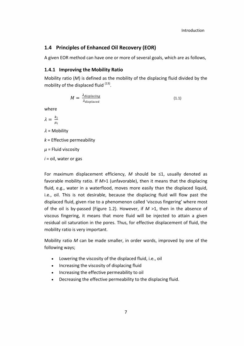
1.4.1 Improving the Mobility Ratio
Mobility ratio (M) is defined as the mobility of the displacing fluid divided by the
mobility of the displaced fluid (13).
(1.1)
where
= Mobility
k = Effective permeability
µ = Fluid viscosity
i = oil, water or gas
For maximum displacement efficiency, M should be ≤1, usually denoted as
favorable mobility ratio. If M>1 (unfavorable), then it means that the displacing
fluid, e.g., water in a waterflood, moves more easily than the displaced liquid,
i.e., oil. This is not desirable, because the displacing fluid will flow past the
displaced fluid, given rise to a phenomenon called ‘viscous fingering’ where most
of the oil is by-passed (Figure 1.2). However, if M >1, then in the absence of
viscous fingering, it means that more fluid will be injected to attain a given
residual oil saturation in the pores. Thus, for effective displacement of fluid, the
mobility ratio is very important.
Mobility ratio M can be made smaller, in order words, improved by one of the
following ways;
Lowering the viscosity of the displaced fluid, i.e., oil
Increasing the viscosity of displacing fluid
Increasing the effective permeability to oil
Decreasing the effective permeability to the displacing fluid.

8
Introduction
1.4.2 Increasing the Capillary Number
The Capillary number, Nc is defined as the dimensionless ratio between the
viscous and the capillary forces, given by (13)
(1.2)
where
= displaced fluid viscosity
= pore velocity
= interfacial tension between the displaced and the displacing fluids
= effective permeability to the displaced fluid
= pressure gradient across distance L
The capillary number can be increased, and thereby the residual oil saturation
decreased, by either reducing oil viscosity or increasing pressure gradient, but
more than anything, by decreasing the interfacial tension (IFT).
Figure 1.2: Water fingering into the oil bank for unfavorable mobility ratios (M >1) (7)

9
Norne Field
2 Norne Field
2.1 General Field Information
The Norne Field is located 200 km from the Norwegian coastline and 85 km north
of Heidrun field. It is situated in the blocks 6608/10 and 6508/1 in the Southern
part of the Nordland II area. The Horst block is approximately 9 km x 3 km. Figure
2.1 shows a map of the location of the Norne field relative to other fields. The
water depth in the area is about 380 m. The field is operated by Statoil ASA and
license partners Eni Norge AS and Petoro.
The Norne field was discovered with well 6608/10-2 in 1991. Based on discovery
well, the total hydrocarbon bearing column of 135 m was found with a 110 m
thick oil leg and 25 m overlying gas cap. The reservoir comprises sandstones of
Middle and Late Jurassic age of excellent quality. These findings were later
confirmed with the appraisal well (6608/10-3) in 1993. The reservoir depth is
about 2500 meters (14; 15).
Figure 2.1: Location of the Norne Field and Field Segments (14)

10
Norne Field
The Norne field consists of two separate oil compartments;
Norne Main Structure (C-, D- and E-segment), discovered in December 1991, containing 97% of the oil in place.
Norne North-East Segment (G-segment) (Figure 2.1)
The Norne main structure is relatively flat containing approximately 80% of oil in
Ile and Tofte formation and gas in the Garn formation above the Not formation
claystone (shale). The underlying water zone is generally in the heterogeneous
Tilje formation and there is no much evidence for aquifer support. The Gas-oil
contact (GOC) is in the vicinity of Not formation Shale which acts as a barrier
throughout the field. This was shown by acquired pressure data from
development wells that increase in pressure in Garn formation and pressure
decline in Ile and Tofte formation, indicating that there is no reservoir
communication across the Not Shale formation during production/injection (14;
16).
2.2 Development
The development drilling began with well 6608/10-D-1 H in August 1996. The oil
production started on November 6th 1997 and oil is being produced by only
water injection as the drive mechanism. In the early days gas was injected, which
was ceased in 2005 and all gas is now being exported. The field has been
developed with six subsea wellhead templates named B, C, D, E, F and K that are
connected to floating production and storage vessel, ‘Norne FPSO’ with flexible
risers. The oil is loaded to tankers for export, while the gas is transported
through pipeline to Åsgard and onward to Kårstø (14; 15)
The NPD has provided the figures in Table 2.1 for the total production,
estimation of recoverable and remaining reserves as of 31st December 2010
(Norwegian share).
Table 2.1: NPD's estimates of recoverable and remaining reserves as of 31.12.2010 (17)
Reserves Oil
(mill Sm3) Gas
(mill Sm3) NGL
(mill ton) Condensate (mill Sm3)
Recoverable 93.40 11.70 1.70 0.00
Produced 84.60 6.20 0.80 0.00
Remaining 8.80 5.50 0.90 0.00

11
Norne Field
2.3 Geology of the Norne Field
The Norne reservoir rock is comprised of Jurassic sandstones, mainly dominated
by fine-grained and well to very well sorted sub-arkosic arenites. The sandstones
are buried at a deep depth of 2500 m to 2700 m and are affected by digenetic
process, which reduces reservoir quality due to mechanical compaction. Even
though, most of the sandstones are of good quality and the porosity is in the
range of 25 % to 30 % while permeability is between 20-2500 mD (15).
2.3.1 Stratigraphy and Sedimentology
The Norne reservoir is classified in two major groups, the FANGST which consists
of the Garn, Not and Ile formations and the BÅT which includes the ROR, Tofte,
Tilje and Åre formations. These formations are further subdivided into sub
formations as shown in Figure 2.2. The Ile and Tofte containing 36% and 44% of
the proven oil respectively are the most important reservoir formations and
therefore will be focused during this thesis work (18).
2.3.1.1 Ile Formation
The Ile formation was deposited during the Aalenian and is 32-40 m thick
sandstone. The formation is divided into three zones; Ile 1, Il 2 and Ile 3. The Ile 1
& Ile 2 and Ile 1 & ROR formations are separated by a cemented calcareous layer
as can be seen in Figure 2.2. These calcareous layers are probably the result of
minor flooding events in a generally regressive period, which might form barrier
to vertical fluid flow and is therefore important in the reservoir modeling (18). The
Ile formation is subdivided into 7 parts (layer 5 to 11) in the reservoir model.
2.3.1.2 Tofte Formation
The Tofte formation was deposited on the top of the unconformity during Late
Toarcian and is approximately 50 meter thick sandstone. As can be seen in Figure
2.2, the formation is divided into three reservoir zones; Tofte 1, 2 and 3. Tofte 1
consists of medium to coarse grained sandstone with variable but generally very
good reservoir properties. In the middle, the Tofte 2 is a composed of muddy and
fine grained sandstone unit and the top represents Tofte 3 which is very fine to
fine grained sandstone (18). The Tofte formation is subdivided into 7 parts (layer
12 to 18) in the reservoir model.

12
Norne Field
Figure 2.2: Stratigraphical sub-division of the Norne reservoir (18)

13
Norne Field
2.4 Reservoir Communication
The Norne Field reservoir consists of both faults and stratigraphic barriers which
act as restrictions to the vertical and lateral flow. In order to better understand
the reservoir communication and drainage pattern during production, vertical
transmissibility multipliers and fault transmissibility multipliers have been
implemented in the reservoir simulation (16).
2.4.1 Faults
As the Norne field is situated on a horst, a number of faults are expected. A horst
is the raised fault block bounded by normal faults or graben. Figure 2.3 shows
the faults and fluid contacts in the Norne Field reservoir.
To describe the faults in the reservoir simulation model, the fault planes are
divided into sections which follow the reservoir zonation. Each sub-area of the
fault planes has been given transmissibility multipliers. The transmissibility
multipliers are functions of fault rock permeability, the matrix permeability, fault
zone width, and dimensions of the grid blocks (16).
2.4.2 Stratigraphic barriers
Numerous stratigraphic barriers are present in the field, which have been
identified and their lateral extent and thickness variation are assessed by the use
of cores and logs. Some of the continuous intervals which restrict the vertical
fluid flow within the Norne Field are:
Garn 3/Garn 2: Carbonate cemented layer at top Garn 2
Not formation: Claystone formation
Ile 3 /Ile 2: Carbonate cementations and increased clay content at the
base Ile 3
Ile 2/Ile 1: Carbonate cemented layer at base Ile 2
Ile 1 / Tofte 4: Carbonate cemented layer at top Tofte 4
Tofte 2 / Tofte 1: Significant grain size constant
Tilje 3 / Tilje 2: Claystone formation
The Not formation is the most prominent barriers to flow, the carbonate
cemented layers which isolates Ile 1 and Tofte 4, and the interbedded claystone
separating the Tilje 3 and Tilje 2 formations (16).

14
Norne Field
Figure 2.3: Structural Cross section through the Norne Field with fluid contacts and faults (16)
2.5 Drainage Strategy
The main goal to develop the Norne was to obtain an economic optimum
production profile. In 2006, the focus was on optimizing the value creation by (19):
Safe and cost effective drainage of proven reserves
Prove new reserves at optimal timing to utilize existing infrastructure
Explore the potential in the license
Adjust capacities where this could be done cost effectively
Improve drainage strategy with low cost infill wells as multilateral/MLT
and through tubing drilled wells (TTRD and TTML).
Increase reservoir pressure in the Ile formation and the Norne G-
segment.

15
Norne Field
Initially, the drainage strategy was to maintain the reservoir pressure by re-
injection of produced gas into the gas cap and water injection into the water
zone. But, during the first year of production it was experienced that the Not
shale is sealing over the Norne Main Structure, so this non-communication
between the Garn and Ile formations made the plan to be revised. The gas
injection was changed to inject in the water zone and the lower part of the oil
zone with proper monitoring to prevent early breakthrough and increase GOR.
The water injection was started in July 1998 and is being injected in the Tilje
formation (water zone). The gas injection was stopped in 2005 and is now being
exported (Figure 2.4 and Figure 2.5) (19).
Figure 2.4 NE-SW cross-section of fluid contacts and drainage strategy for the Norne Field (19)
Figure 2.5: The drainage strategy for the Norne Field from pre-start to 2014 (19)

16
Norne Field E-Segment
3 Norne Field E-Segment
The Norne E-segment is a part of the Norne main structure (C-, D- and E-
segment). The Ile and the Tofte are the key formations in this segment because
80% oil in the Norne field is contained in these formations. The E-segment is
separated from the rest of the field on an assumption of a constant flux
boundary. This means that we have considered a hypothetical boundary across
which the flow of fluid flowing into the E-segment is equal to the liquid flowing
out. Hence any change in any other segment of reservoir, theoretically will have
no effect on any parameter inside the reservoir.
In the Eclipse model of Norne Field, the E-segment consists of 3 producers and 2
injectors as on 2004 (Table 3.1).
Table 3.1: Wells Status in the Norne field E-Segment
Well Name Type Status
F-1H Water Injector (vertical) Active
F-3H Water Injector (vertical) Active
E-2H Oil Producer (horizontal) Active
E-3H Oil Producer (vertical) Shut
E-3AH Oil Producer (horizontal) Active
3.1 The Reservoir Simulation Model
The Norne field is modeled in Eclipse 100; a fully implicit, three phase, three
dimensional black oil simulator. The reservoir model has 46 grids in the X-
direction, 112 in the Y-direction and 22 layers. Each geological layer (reservoir
zone) is represented by one layer, for example, the Ile is represented by layers 5-
11 and Tofte by 12-18. The model used in this study is a coarsened model which
is made from the original full field reservoir simulation model by Mohsen
Dadashpur at the IO Center. Figure 3.1 shows a coarsened model where only E-
segment is fine gridded (blue color). The simulation with history matched runs
from November 1997 until December 2004 (15). Norne’s fluid properties are given
in Table 3.2.

17
Norne Field E-Segment
Table 3.2: Fluid parameters for the Norne Field (20)
Fluid Properties Units Norne Main Structure (C,D & E Segment)
Norne G-Segment
Initial pressure bar 273.2 273.2
Bubble point pressure bar 251 216
Gas oil ratio Sm3/Sm3 111 96
Oil formation volume factor at bubble point
Rm3/Rm3 1.347 1.30
Oil viscosity at bubble point cp 0.58 0.695
Oil density at bubble point g/cm3 0.712 0.729
Gas formation volume factor
Rm3/Rm3 4.74 E-3
Initial temperature 0C 98.3 98.3
Figure 3.1 The coarsened simulation model of Norne Field showing E-segment

18
Norne Field E-Segment
3.2 EOR Potential in Norne E-segment
Petrophysical and geological data shows that approximately 80% of the oil
reserves in the Norne E-segment are located in Ile and Tofte formation; therefore
these two formations are selected as the target area for EOR (18).
In the eclipse model, the Ile and Tofte formations are represented by 5-18 layers.
The simulation was run from 1997 till 2004, and it can be seen from Figure 3.4
and Figure 3.5, the oil saturation is still very high in the Ile formation. Tofte
formation has comparatively low oil saturation (Figure 3.6). The recovery factor
and oil in place of the history matched model are shown in Figure 3.2 and Figure
3.3, where pink line represents history and blue line as prediction. The recovery
factor and oil-in-place are 41.30 % and 1.60 x 10⁶ sm3 in November 2004 and
with future predictions these are recorded as around 54.30 % and 1.24 x 10⁶ sm3
respectively in December 2015. A recovery factor at 54.30 % is an excellent result
with only water flooding, which means that sweep efficiency in the E-segment is
very good. As shown in Figure 3.4 and Figure 3.5, the pockets of oil are still
trapped in the Norne E-segment after water flooding for a number of years,
which means that this can be a good candidate of suitable EOR method.
Figure 3.2: Recovery factor for the Norne E-Segment
Figure 3.3: Oil-in-place for the Norne E-Segment

19
Norne Field E-Segment
Figure 3.4: Oil saturation in the Ile formation (layer 5), November 2004
Figure 3.5: Oil saturation in the Ile formation (layer 8), November 2004
Figure 3.6: Oil saturation in the Tofte formation (layer 12), November 2004

20
Norne Field E-Segment
3.3 EOR Screening Criteria of the Norne E-Segment
Screening criteria have been widely used to identify EOR applicability in a
particular field before any detailed evaluation is started. EOR screening
represents a key step to reducing the number of options for further detailed
evaluations. Over the past two decades, many researchers- for example, Taber et
al. (1997a, 1997b), Al-Bahar et al. (2004), Henson et al. (2002) and Dickson et al.
(2010) have developed detailed economic and technical screening criteria for
different EOR processes through modeling/simulation and using laboratory and
field data (2). To perform the EOR screening on the Norne E-segment, we will use
the screening criteria of Taber et al. (1). Table 3.3 shows the summary of
screening criteria which is based on a combination of the reservoir and oil
characteristics of successful projects plus the optimum conditions needed for
good oil displacement by the different fluids. The suggested criteria in Table 3.3
are informative and intended to show approximate ranges of good projects but
they may be misleading (1).
According to Taber et al., a convenient way to show different EOR methods is to
arrange them by oil gravity as shown in Figure 3.7. The size of the type in Figure
3.7 illustrates the relative importance of each of the EOR methods in terms of
incremental oil produced (1).
The reservoir and oil characteristics used for EOR screening of Norne E-segment
are presented in Table 3.4. The API gravity of Norne oil is 32.7o and the other
parameters like oil saturation, formation type, net thickness, permeability and
depth given in Table 3.4 almost satisfy the characteristics for chemical methods
given in Table 3.3 and Figure 3.7, whereas the Norne oil viscosity is lower and
temperature is slightly higher (5 oC more) than the range suggested in Table 3.3.
The author in the light of above discussion decided to simulate chemical
methods (alkaline, surfactant and/or polymer) for the Norne E-segment because
the current drainage strategy is water flooding, which is also an advantageous for
these methods. However, the chemical EOR processes are complex and
expensive, high adsorption and degradation of chemicals can occur at high
temperatures.

21
Norne Field E-Segment
Table 3.3: Summary of screening criteria for EOR Methods (1; 7)
Table 3.4 : Reservoir and oil parameters for the Norne Field (14; 16; 8)
Reservoir Characteristics Oil Properties
Permeability, mD 20-2500 Gravity (API) 32.7o
Porosity, % 25-30 Viscosity, cp <1.2
Formation type Sandstone Density, kg/m3 859.5
Net thickness, m 110
Reservoir Depth, m 2500-2700
Temperature, oC 98.3
Oil Saturation, % 35-92
Figure 3.7: Oil gravity range of oil that is most effective for EOR methods (1)

22
Overview of Surfactant, Alkaline and Polymer Flooding
4 Overview of Surfactant, Alkaline and Polymer Flooding
4.1 Surfactant Flooding
The term surfactant is a blend of surface acting agents that adsorb on or
concentrate at a surface or fluid/fluid interface to alter the surface properties
significantly; in particular, they decrease surface tension or interfacial tension
(IFT). Surfactants are usually organic compounds that are amphiphilic (Figure
4.1), meaning they are made up of two functional groups, hydrophobic (water-
hating, the “tail”) and polar hydrophilic (water-loving, the “head”). Due to this
nature, they are soluble in both organic solvents and water (2).
4.1.1 Basic Surfactant Classification
Surfactants are categorized into four groups according to the ionic nature of
head group as anionic, nonionic, cationic and Zwitterionic (amphoteric).
1. Anionic This surfactant is classified as anionic because of the negative charge on its head
group. They are most widely used in chemical EOR processes because they are
stable, efficiently reduce IFT, relatively resistant to retention, exhibit relatively
low adsorption on sandstone rocks whose surface charge is negative. Anionic
surfactants can strongly adsorb in carbonate rocks (having positive surface
charge), therefore, they are not used in carbonate rocks.
2. Nonionic Nonionic surfactants have no charge and primarily serve as co-surfactants to
improve the phase behavior. They are more tolerant of high salinity brine, but
their surface active properties to reduce IFT are not as good as anionic
surfactants. Mostly, a mixture of anionic and nonionic is used to increase the
tolerance to salinity.
3. Cationic Cationic surfactants are positively charged and they strongly adsorb in sandstone
rocks; therefore, they are not used in sandstone reservoirs, but they can be used
in carbonate rocks to change wettability from oil-wet to water-wet.
4. Zwitterionic Zwitterionic surfactants also known as amphoteric (positive and negative
charges) contain two active groups. The types of zwitterionic surfactants can be

23
Overview of Surfactant, Alkaline and Polymer Flooding
nonionic-anionic, nonionic-cationic, or anionic-cationic. These surfactants are
expensive because they are temperature and salinity-tolerant (2; 21).
Figure 4.1: Representative surfactant molecular structures (22)
Figure 4.2: Classification of surfactants and examples (23)
4.1.2 Methods to Characterize Surfactants
The most common surfactants used in surfactant flooding are petroleum
sulfonates. These are anionic surfactants produced when an intermediate-
molecular-weight refinery stream is sulfonated, and synthetic sulfonates are the
products when a relatively pure organic compound is sulfonated. Sulfonates are
stable at high temperatures but sensitive to divalent ions (2). Several methods to
characterize surfactants are discussed next.

24
Overview of Surfactant, Alkaline and Polymer Flooding
4.1.2.1 Hydrophile–Lipophile Balance (HLB)
The hydrophile–lipophile balance (HLB) number indicates the tendency to form
water-in-oil or oil-in-water emulsions. Low HLB numbers are assigned to
surfactants that tend to be more soluble in oil and to form water-in-oil
emulsions. When the formation salinity is low, a low HLB surfactant should be
selected. Such a surfactant can make middle-phase microemulsion at low
salinity. When the formation salinity is high, a high HLB surfactant should be
selected. Such a surfactant is more hydrophilic and can make middle-phase
microemulsion at high salinity (2).
4.1.2.2 Critical Micelle Concentration
CMC is defined as the concentration of surfactants above which micelles are
spontaneously formed. Micelle is an aggregation of molecules which usually
consists of 50 or more surfactant molecules. When surfactants are injected into
the system, they will initially partition into the interface, reducing the system
free energy by lowering the energy of the interface and removing the
hydrophobic parts of the surfactant from contact with water. As the
concentration of surfactant increases and the surface free energy (surface
tension) decreases, the surfactants start aggregating into micelles. Above a
specific concentration, called as critical micelle concentration (CMC), further
addition of surfactants will just increase number of micelles as shown in Figure
4.3. In other words, before reaching the CMC, the surface tension decreases
sharply with the concentration of the surfactant whereas the surface tension
stays more or less constant after reaching the CMC (2; 21).
Figure 4.3: Schematic definition of the critical micelle concentration (CMC) (22)

25
Overview of Surfactant, Alkaline and Polymer Flooding
4.1.2.3 Solubilization Ratio
Solubilization is the process of making a normally insoluble material soluble in a
given medium. Solubilization ratio for oil (water) is defined as the ratio of the
solubilized oil (water) volume to the surfactant volume in the microemulsion
phase. Huh (1979) formulated that solubilization ratio is closely related to IFT.
When the solubilization ratio for oil is equal to that for water, the IFT reaches its
minimum (2).
4.1.3 Surfactant Flooding in Petroleum Reservoirs
The purpose of surfactant flooding is to recover the capillary trapped oil after
water flooding. When a surfactant solution has been injected, the trapped oil
droplets are mobilized due to a reduction in the interfacial tension between oil
and water. The coalescence of these drops leads to a local increase in oil
saturation and oil bank is generated. The oil bank will start to flow, mobilizing
any residual oil in front of the bank. Behind the flowing oil bank, the surfactant
will prevent the mobilized oil to be re-trapped. The interfacial tension, the
viscosity, and the volume of the surfactant solution behind the oil bank will
therefore be of importance for the final residual oil saturation.
If the efficiency of surfactant is very good, then the reduction in Interfacial
tension (IFT) could be as much as 104 which corresponds to a value in the
neighborhood of 1μN/m. Due to high cost of surfactant, mostly a small surfactant
slug is displaced by water, usually containing polymer to increase viscosity which
prevents fingering and breakdown down of slug (24). The main aspects of
surfactant flooding are discussed below;
4.1.3.1 Capillary Desaturation Curve (CDC)
To reduce waterflood residual oil saturation, the pressure drop across the
trapped oil has to overcome the capillary forces that keep the oil trapped. This is
done with surfactant which provides such a pressure drop. A large number of
studies have shown that the residual oil saturation corresponds to the capillary
number (Nc), the dimensionless ratio between the viscous and capillary forces. In
general, the capillary number must be higher than a critical capillary number,
(NC)c, for a residual phase to start to mobilize. Practically, this (NC)c is much
higher than the capillary number at normal waterflooding conditions. Another
parameter is maximum desaturation capillary number, (NC)max, above which the

26
Overview of Surfactant, Alkaline and Polymer Flooding
residual saturation would not be further decreased in practical conditions even if
the capillary number is increased (2; 24).
The general relationship between residual saturation of a non-aqueous
(nonwetting phase) or aqueous phase (wetting phase) and a local capillary
number is called capillary desaturation curve (CDC). The residual saturations start
to decrease at the critical capillary number as the capillary number increases,
and cannot be decreased further at the maximum capillary number (Figure 4.4).
The CDC for the wetting phase is shifted to the right of the CDC of the non-
wetting phase by two orders of magnitude (see Figure 4.4); this indicates that
surfactant should have better performance in a water-wet system. Figure 4.5
shows that oil saturation starts to drop as pore size becomes narrower at high
capillary number (NC), which means that a reservoir with narrow pore-size
distribution will give the lowest residual oil saturation. In a simulation model, the
efficiency of the surfactant will rely upon CDC, and should therefore be
measured for every distinct rock type (2; 24).
Figure 4.4: Effect of wettability on residual saturation of wetting and non-wetting phase (24)

27
Overview of Surfactant, Alkaline and Polymer Flooding
Figure 4.5: Effect of pore-size distribution on the CDC (24)
4.1.3.2 Volumetric Sweep Efficiency and Mobility Ratio
Volumetric sweep efficiency Ev is the volume of oil contacted divided by the
volume of target oil. Ev is a function of surfactant/polymer slug size, retention
and heterogeneity. The mobility ratio has to be as low as possible for an efficient
displacement of the oil bank towards the producing wells. Low mobility ratio
prevents fingering of the surfactant slug into the oil bank and also reduces large-
scale dispersion due to permeability contrasts, gravity segregation and well
pattern. The mobility control agent in the slug can be a polymer or oil. It is of
paramount importance that the slug-oil bank front be made viscosity stable since
small slugs cannot tolerate even a small amount of fingering. It has been
confirmed from simulation studies that low mobility ratio is of great importance
according to recovery, while the size of the surfactant slug gave small differences
in performance (22; 24).
4.1.3.3 Relative Permeabilities
In chemical flooding process, relative permeability is most likely one of the least-
defined parameters. The classic relative permeability curves represent a situation
in which fluid distribution in the system is controlled by capillary forces (2). The
concept of relative permeability is fundamental to the study of the simultaneous

28
Overview of Surfactant, Alkaline and Polymer Flooding
flow of immiscible fluids in porous media. Relative permeabilities are influenced
by the following factors; saturation, saturation history, wettability, temperature,
viscous, capillary and gravitational forces (7).
In surfactant-related processes, the interfacial tension is reduced. As IFT is
reduced, the capillary number is increased, leading to reduced residual
saturations. Obviously, residual saturation reduction directly changes relative
permeabilities and the relative permeability curves become closer to straight
lines (exponents close to 1), and the immobile saturations are closer to 0.
Many researchers observed from their experimental results that as water/oil IFT
was reduced, both oil and water relative permeabilities were increased, their end
points were raised, had less curvature, and residual saturations were decreased.
These observations were obvious only when the IFT was below 0.1 mN/m (2).
4.1.3.4 Surfactant Retention
Control of surfactant retention in the reservoir is one of the most important
factors in determining the success or failure of a surfactant flooding project.
Based on the mechanisms, surfactant retention has been identified as
precipitation, adsorption, and phase trapping. These mechanisms all result in
retention of surfactant in a porous medium and deterioration of the composition
of the chemical slug, leading to poor displacement efficiency. Surfactant
retention in reservoirs depends on surfactant type, surfactant equivalent weight,
surfactant concentration, rock minerals, clay content, temperature, pH, flow rate
of the solution, etc. As the equivalent weight of the surfactant increases,
surfactant retention in general also increases (2). Petroleum sulfonates are widely
used in surfactant flooding. The presence of divalent cations (Ca2+, Mg2+) in the
solution causes surfactant precipitation.
Adsorption
Most solid surfaces including reservoir rocks are charged due to different
mineralogy. The reservoir minerals like quartz (silica), kaolinite show a negative
charge while calcite, dolomite and clay have positive charge on their surfaces at
neutral pH of the brine. The adsorption of surfactants at the solid/liquid interface
comes into play by electrostatic interaction between the charged solid surface
(adsorbent) and the surfactant ions (adsorbate). Ion exchange, ion pairing and
hydrophobic bonding are some of mechanisms by which surfactants adsorb onto
mineral surfaces of rock (7). Nonionic surfactants have much higher adsorption on

29
Overview of Surfactant, Alkaline and Polymer Flooding
a sandstone surface than anionic surfactants whereas for calcite is reverse. Thus,
nonionic surfactants might be candidates for use in carbonate formations from
the adsorption point of view (2; 25).
An example of an isotherm for the adsorption of a negatively charged surfactant
onto an adsorbent with positively charged sites is S-shaped. Figure 4.6 shows
four different regions reflecting distinct modes of adsorption (24).
Region 1: In this region, the surfactant is mainly adsorbed by anionic exchange
and shows a linear relationship between adsorbed material and equilibrium
concentration.
Region 2: A remarkable increase in adsorption due to the interaction between
the hydrophobic chains of the oncoming surfactant and the surfactant that
already has been adsorbed.
Region 3: A decrease in adsorption of surfactants because the adsorption has to
overcome the electrostatic repulsion between surfactant and the similarly
charged solid.
Region 4: A plateau adsorption is obtained above the Critical Micelle
Concentration (CMC), which means that surfactant adsorption will not increase
onto the surface.
The interfacial tension between oil and water decreases until the CMC is
reached. The shape of the adsorption isotherm may vary for different systems,
and some factors that influence the plateau are salinity, pH-value, temperature
and wettability. With increased salinity the plateau adsorption will increase while
a decrease in pH will cause an increase in adsorption. It is suggested that
surfactant adsorption decrease as the temperature increases (8).

30
Overview of Surfactant, Alkaline and Polymer Flooding
Figure 4.6: Schematic S-shaped adsorption curve (24)
One of the ways of reducing adsorption in chemical flooding is by doing a ‘pre-
flush’ with different type of sacrificial chemicals like NaCl, NaOH, phosphates,
silicates, lignosulfonates and polyethylene oxide in order to reduce hardness,
make the reservoir rock more negative charged and block the active sites of the
rock (24).
Phase Trapping
This form of retention is strongly affected by the phase behavior. Phase trapping
could be caused by mechanical trapping, phase partitioning, or hydrodynamical
trapping. It is related to multiphase flow. The mechanisms are complex, and the
magnitude of surfactant loss owing to phase trapping could be quite different
depending on multiphase flow conditions. Glover et al. (1979) found that the
onset of phase trapping with a surfactant flooding process generally occurred at
higher salt concentrations because it would form upper-phase microemulsion so
that the surfactant would be trapped in the residual oil. Krumrine (1982)
proposed that the addition of alkali would reduce the concentration of hardness
ions that may cause surfactant retention. Therefore, ASP will have little
surfactant retention due to ion exchange (25).

31
Overview of Surfactant, Alkaline and Polymer Flooding
4.2 Polymer Flooding
Mobility control is one of the most important concepts in any enhanced oil
recovery process. It can be achieved through injection of chemicals to change
displacing fluid viscosity or to preferentially reduce specific fluid relative
permeability through injection of foams. The commonly used mobility control
agent is polymer because it can significantly increase the apparent viscosity of
the injected fluid. Foam is also a good mobility control method with water,
surfactant and gas, but here we will only focus on polymer (2).
Polymer flooding consists of adding polymer to the water of a waterflood to
decrease its mobility. The resulting increase in viscosity, as well as a decrease in
aqueous phase permeability, causes a lower mobility ratio. This lowering
increases the volumetric sweep efficiency and lower swept zone oil saturation.
The polymer flooding will be economic and useful only when the waterflood
mobility ratio is high, the reservoir heterogeneity is serious, or a combination of
these two happens (22).
Polymer flooding can yield a significant increase in oil recovery compared to
conventional water flooding techniques. A typical polymer flood project involves
mixing and injecting polymer over an extended period of time until about 1/3–
1/2 of the reservoir pore volume has been injected. This polymer “slug” is then
followed by continued long term water flooding to drive the polymer slug and
the oil bank in front of it toward the production wells. Polymer is injected
continuously over a period of years to reach the desired pore volume (26).
Polymers are often used with surfactant and alkali agents to improve volumetric
sweep efficiency, reduce channeling and breakthrough and they can also provide
mobility control at the low IFT front. Otherwise, the front is not stable and will
finger and dissipate. Figure 4.7 shows the fingering effect with water flooding
while use of polymers (Figure 4.8) has reduced the effect of fingering
significantly.
4.2.1 Types of Polymers
Two main types of polymers, synthetic polymers such as hydrolyzed
polyacrylamide (HPAM) and biopolymers such as xanthan gum are commonly
used in enhanced oil recovery. Less commonly used are natural polymers and
their derivatives, such as guar gum, sodium carboxymethyl cellulose, and
hydroxyl ethyl cellulose (HEC).

32
Overview of Surfactant, Alkaline and Polymer Flooding
Figure 4.7: Fingering effect with water flooding (27)
Figure 4.8: Decreased effects of fingering with polymer flooding (27)
4.2.1.1 Hydrolyzed Polyacrylamide (HAPM)
HPAM is the most widely used polymer in EOR applications. In China’s Daqing
field, HPAM solutions have provided significantly greater oil recovery for either a
given polymer concentration or viscosity level. The reason is that HPAM solutions
exhibit significantly greater viscoelasticity than xanthan solutions. Polyacrylamide
adsorbs strongly on mineral surfaces, therefore it is partially hydrolyzed to
reduce adsorption by reacting polyacrylamide with a base (sodium or potassium
hydroxide or sodium carbonate) (2). Hydrolysis converts some of the amide
groups (CONH2) to carboxyl groups (COO−), as shown in Figure 4.9.
Figure 4.9: Partially hydrolyzed polyacrylamide (22)

33
Overview of Surfactant, Alkaline and Polymer Flooding
Typical degrees of hydrolysis are 15 to 35% of the acrylamide monomers; hence
the HPAM molecule is negatively charged that have a large effect on the
rheological properties of the polymer solution. According Green and Willhite
(1998), polyacrylamide is mainly anionic, but could be nonionic or cationic. The
molecular weights of HPAM used in EOR processes are up to higher than 20
million Daltons (2; 22).
Advantages/disadvantages: They are relatively cheap, develop high viscosities in
fresh water, and adsorb on the rock surface to give a long-term permeability
reduction. The main disadvantages are their tendency to shear degradation at
high flow rates, sensitive to high temperature and their poor performance in high
salinity brine.
4.2.1.2 Xanthan Gum
Another widely used polymer, a biopolymer, is xanthan gum (corn sugar gum).
These polymers are formed from the polymerization of saccharide molecules, a
bacterial fermentation process. The structure of a xanthan biopolymer is shown
in Figure 4.10. Xanthan gum has a more rigid structure and is quite resistant to
mechanical degradation. These properties make it relatively insensitive to salinity
and hardness. It is susceptible to bacterial attack after it has been injected into
the reservoir. The polymer is relatively nonionic and, therefore, free of ionic
shielding effects of HPAM. Molecular weights of xanthan biopolymer used in EOR
processes are in range of 1 million to 15 million.
Xanthan is supplied as a dry powder or as a concentrated broth. It is often
chosen for a field application when no fresh water is available for flooding. Some
permanent shear loss of viscosity could occur for polyacrylamide, but not for
polysaccharide at the wellbore. However, the residual permeability reduction
factor of polysaccharide polymers is low. Other potential EOR biopolymers are
scleroglucan, simusan, alginate, etc (2; 22).
Figure 4.10: Molecular structure of Xanthan

34
Overview of Surfactant, Alkaline and Polymer Flooding
4.2.2 Polymer Flow Behavior in Porous Media
4.2.2.1 Polymer Retention
Retention of polymer in a reservoir includes adsorption, mechanical trapping,
and hydrodynamic retention. Adsorption refers to the interaction between
polymer molecules and the solid surface. This interaction causes polymer
molecules to be bound to the surface of the solid, mainly by physical adsorption,
and hydrogen bonding. Mechanical entrapment and hydrodynamic retention are
related and occur only in flow-through porous media. Retention by mechanical
entrapment occurs when larger polymer molecules become lodged in narrow
flow channels. The level of polymer retained in a reservoir rock depends on
permeability of the rock, nature of the rock (sandstone, carbonate, minerals, or
clays), polymer type, polymer molecular weight, polymer concentration, brine
salinity, and rock surface (2; 22).
4.2.2.2 Inaccessible Pore Volume
When size of polymer molecules is larger than some pores in a porous medium,
the polymer molecules cannot flow through those pores. The volume of those
pores that cannot be accessed by polymer molecules is called inaccessible pore
volume (IPV) (2). The inaccessible pore volume is a function of polymer molecular
weight, medium permeability, porosity, salinity, and pore size distribution. In
extreme cases, IPV can be 30% of the total pore volume (22).
4.2.2.3 Permeability Reduction and the Resistance Factor
Polymer adsorption/retention causes the reduction in apparent permeability.
Therefore, rock permeability is reduced when a polymer solution is flowing
through it, compared with the permeability when water is flowing. This
permeability reduction is defined by the permeability reduction factor (Rk) (2):
(4.1)
The resistance factor (Rf) is defined as the ratio of mobility of water to the
mobility of a polymer solution flowing under the same conditions.
(4.2)
The residual resistance factor (Rrf) is the ratio of the mobility of water before to
that after the injection of polymer solution (22).

35
Overview of Surfactant, Alkaline and Polymer Flooding
(4.3)
Residual resistance factor is a measure of the tendency of the polymer to adsorb
and thus partially block the porous medium. Permeability reduction depends on
the type of polymer, the amount of polymer retained, the pore-size distribution,
and the average size of the polymer relative to pores in the rock (21).
4.2.2.4 Relative Permeabilities in Polymer Flooding
Some of the researchers have proved from their experiments that polymer
flooding does not reduce residual oil saturation in a micro scale. The polymer
function is to increase displacing fluid viscosity and thus to increase sweep
efficiency. Also, fluid viscosities do not affect relative permeability curves.
Therefore, it is believed that the relative permeabilities in polymer flooding and
in water flooding after polymer flooding are the same as those measured in
waterflooding before polymer flooding (2).
4.2.2.5 Polymer Rheology in Porous Media
The rheological behavior of fluids can be classified as Newtonian and Non-
Newtonian. Water is a Newtonian fluid in that the flow rate varies linearly with
the pressure gradient, thus viscosity is independent of flow rate. Polymers are
Non-Newtonian fluids. Rheological behavior can be expressed in the terms of
‘apparent viscosity’ which can be defined as
(4.4)
where
= shear stress
= shear rate
The apparent viscosity of polymer solutions used in EOR processes decreases as
shear rate increases. Fluids with this rheological characteristic are said to be
shear thinning. Materials that exhibit shear thinning effect are called
pseudoplastic. Polysaccharides such as Xanthan are not shear sensitive and even
high shear rate is employed to Xanthan solutions to obtain proper mixing, while
polyacrylamides are more shear sensitive. Most significant change in polymer
mobility occurs near the wells where fluid viscosities are large (21).

36
Overview of Surfactant, Alkaline and Polymer Flooding
4.3 Alkaline Flooding
The alkaline flooding method relies on a chemical reaction between high-pH
chemicals such as sodium carbonate and sodium hydroxide (most common alkali
agents) and organic acids (saponifiable components) in crude oil to produce in
situ surfactants (soaps) that can lower interfacial tension. In most of the
literature, these saponifiable components are described as petroleum acids, even
though their structure is not known. The addition of the alkali increases pH and
lowers the surfactant adsorption so that very low surfactant concentrations can
be used to reduce cost. This process is generally applied with crude oils of
relatively low API gravity and containing high acidic components (2).
Mobility control can improve displacement efficiency in alkaline floods. For this,
mostly polymer is used as a mobility buffer to displace the primary slug. In
addition, the reservoir is also conditioned with preflush before the injection of
primary slug (21).
Alkaline flooding is also called caustic flooding. Most commonly used alkalis for in
situ generation of surfactants are sodium hydroxide, sodium carbonate, sodium
orthosilicate, sodium tripolyphosphate, sodium metaborate, ammonium
hydroxide, and ammonium carbonate. Nowadays, ASP formulations use
moderate pH chemicals such as sodium bicarbonate (NaHCO3) or sodium
carbonate (Na2CO3) instead of sodium hydroxide (NaOH) to reduce emulsion and
scale problems. Chinese Daqing oil field ASP projects have had difficulty in
breaking emulsion when using a strong alkali such as NaOH.
Addition of the alkali chemicals results in a high pH because of the dissociation in
the aqueous phase. High pH indicates large concentration of hydroxide ions
(OH-). For example, NaOH dissociates to yield (OH-) as below:
(4.5)
Sodium carbonates dissociates as
(4.6)
followed by the hydrolysis reaction
(4.7)
In carbonate reservoirs where anhydrite (CaSO4) or gypsum (CaSO4·2H2O) exists,
the CaCO3 or Ca(OH)2 precipitation occurs when Na2CO3 or NaOH is added.

37
Overview of Surfactant, Alkaline and Polymer Flooding
Carbonate reservoirs also contain brine with a higher concentration of divalents
and could cause precipitation. To overcome this problem, Liu (2007) suggested
NaHCO3 and Na2SO4. NaHCO3 has a much lower carbonate ion concentration,
and additional sulfate ions can decrease calcium ion concentration in the
solution (2).
4.3.1 Alkaline Reaction with Crude Oil
4.3.1.1 In Situ Soap Generation
In alkaline flooding, the injected alkali reacts with the saponifiable components
in the reservoir crude oil. These saponifiable components are described as
petroleum acids (naphthenic acids). Naphthenic acid consists of carboxylic acids,
carboxyphenols, porphyrins, and asphaltene with molecular weight of 120 to well
over 700. If the crude oil contains an acidic hydrocarbon component then
hydroxide ion must react with a pseudo-acid component (HA) to form a
surfactant. If no HA is originally present in the crude oil, little surfactant can be
generated. A useful procedure for identifying crudes for their attractiveness to
alkaline flooding is through acid number which (also called total acid number,
TAN) is a measure of the potential of a crude oil to form surfactants. The acid
number is the mass of potassium hydroxide (KOH) in milligrams required to
neutralize one gram of crude oil. The alkali–oil chemistry is described by
partitioning of this pseudo-acid component between the oleic and aqueous
phases (equation 4.9) and subsequent hydrolysis in the presence of alkali to
produce a soluble anionic surfactant A-, as shown in Figure 4.11 (2).
The overall hydrolysis and extraction are given by
(4.8)
The extent of equation 4.8 reaction depends strongly on the aqueous solution
pH. This reaction occurs at the water/oil interface. A fraction of organic acids in
oil become ionized with the addition of an alkali, whereas others remained
electronically neutral. The hydrogen-bonding interaction between the ionized
and neutral acids can lead to the formation of a complex called acid soap. Thus,
the overall reaction, equation 4.8, is decomposed into a distribution of the
molecular acid between the oleic and aqueous phases,
(4.9)
and an aqueous hydrolysis,

38
Overview of Surfactant, Alkaline and Polymer Flooding
(4.10)
where, HA denotes a single acid species, A- denotes anionic surfactant, and
subscripts o and w denote oleic and aqueous phases, respectively (2).
Figure 4.11 : Schematic of alkaline recovery process (2)
4.3.1.2 Emulsification
Alkaline chemicals can cause improved oil recovery through the formation of
emulsions. In alkaline flooding, emulsification is instant, and emulsions are very
stable. Emulsification mainly depends on the water/oil IFT. The lower the IFT, the
easier the emulsification occurs. The stability of an emulsion mainly depends on
the film of the water/oil interface. The acidic components in the crude oil could
reduce IFT to make emulsification occur easily, whereas the asphaltene
surfactants adsorb on the interface to make the film stronger so that the stability
of emulsion is enhanced. Local formation of highly viscous emulsions is not
desirable since these would promote viscous instability (2; 22).

39
Overview of Surfactant, Alkaline and Polymer Flooding
4.4 Alkaline Surfactant Polymer (ASP) Flooding
Alkaline-Surfactant-Polymer (ASP) flooding has been recognized to be one of the
major EOR techniques that can be successfully used in producing light and
medium oils left in the reservoirs after primary and secondary recovery (28). The
success of this method depends on the identification of the proper alkali,
surfactant, and polymer and on the way they are combined to produce
compatible formulation that yields good crude oil emulsification / mobilization,
low chemical losses and good mobility control (29). The synergistic effect of
alkaline, surfactant and polymer results in less surfactant required to recover
significantly incremental oil. An ASP flood involves injecting a predetermined
pore volume of ASP slug into the reservoir. Typically, the ASP formulation
consists of about 0.5-1% alkali, 1% surfactant, and 0.1% polymer. The alkali
reacts with acidic components in the crude oil creating natural soap and also
helps with reducing the adsorption of the surfactant on the rock. It also alters
rock wettability (from oil-wet to water-wet) and adjusts pH and salinity.
Surfactant component helps in releasing the oil from the rock by reducing the
interfacial tension between oil and water while polymer acts as viscosity modifier
and helps mobilize the oil. Often, the ASP slug is followed by polymer “push”
solution for conformance control, mobility control (reduce fingering). This also
helps reduce the slope of oil recovery decline and helps extend the production
for a longer period of time. Upon the completion of polymer injection, driving
fluid (water) is injected to move the chemicals and resulting oil bank towards
production wells. Generally, the reservoir is conditioned by preflush (with water,
alkali or polymer depending on rock mineralogy) before the injection of ASP slug
into reservoir (30). Figure 4.12 shows the typical ASP flooding process in a 5-spot
well pattern.
Displacement mechanisms in ASP may be summarized as follows (2):
Increased capillary number effect to reduce residual oil saturation
because of low to ultralow IFT.
Surfactant adsorption is reduced on both sandstones and carbonates at
high pH.
High pH also improves microemulsion phase behavior.
Improved macroscopic sweep efficiency because of the viscous polymer
drive.
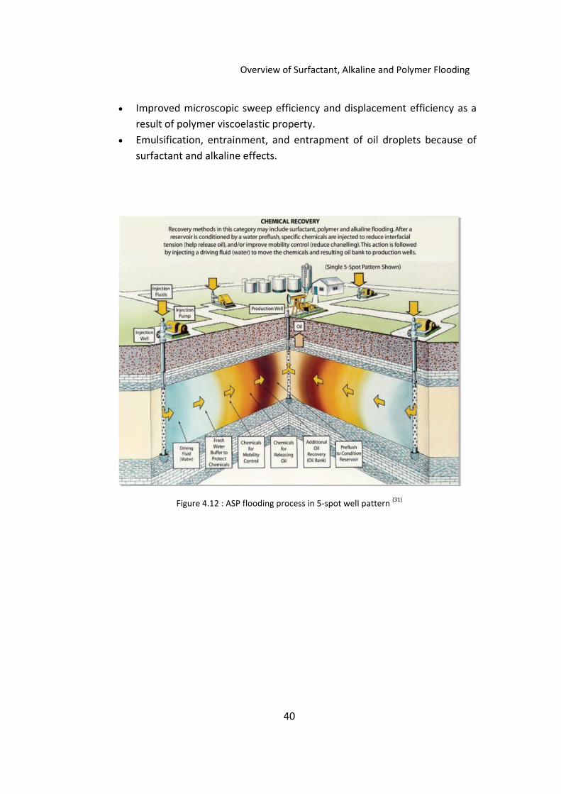
40
Overview of Surfactant, Alkaline and Polymer Flooding
Improved microscopic sweep efficiency and displacement efficiency as a
result of polymer viscoelastic property.
Emulsification, entrainment, and entrapment of oil droplets because of
surfactant and alkaline effects.
Figure 4.12 : ASP flooding process in 5-spot well pattern (31)

41
Simulation of Alkaline, Surfactant and Polymer Flooding
5 Simulation of Alkaline, Surfactant and Polymer Flooding
Different chemical EOR methods such as surfactant flooding, alkaline-surfactant
(AS) flooding, polymer flooding, surfactant-polymer (SP) flooding, and alkaline-
surfactant-polymer (ASP) flooding in Norne E-segment were simulated using
Eclipse-100. The economic evaluations were performed based on the
incremental oil recovery over water flooding using the Net Present Value (NPV)
model.
5.1 The Surfactant Flood Model
Eclipse 100 does not provide the detailed chemistry of a surfactant process, but
models the important features of a surfactant flood on a full field basis. It does
not provide options as to what type of surfactant to use for given reservoir
structures or certain fluid characteristics. It just presents the surfactant option as
a blanket over all types of reservoir and fluid characteristics. The injected
surfactant is modeled by solving a conservation equation for surfactant within
the water phase. The surfactant concentrations are updated fully-implicitly at the
end of each time-step after the oil, water and gas flows have been computed.
The surfactant is assumed to exist only in the water phase, and the input to the
reservoir is specified as a concentration at water injector (32). The detailed
description of the surfactant model is presented in Appendix A.
5.2 The Polymer Flood Model
The Polymer Flood option uses a fully implicit five-component model (oil/ water/
gas/ polymer/ brine) to allow the detailed mechanisms involved in polymer
displacement process to be studied. The flow of the polymer solution through
the porous medium is assumed to have no influence on the flow of the
hydrocarbon phases (32). A full description of the polymer model can be found in
Appendix B.
5.3 The Alkaline Flood Model
The Eclipse 100 does not take into account the in-situ surfactant creation and the
phase behavior. This simplified model is targeted at looking at some of the
effects of the alkaline on an ASP flooding performance and also to analyze its
effect on the water-oil surface tension and adsorption reduction of surfactant

42
Simulation of Alkaline, Surfactant and Polymer Flooding
and polymer (32). A more detailed description of the alkaline model is given in
Appendix C.
5.4 Alkaline, Surfactant and Polymer Properties
The current drive mechanism for Norne field is water flooding and there has
been no study of chemical EOR for the field. Therefore, the chemical properties
(alkali, surfactant and polymer) used in this study are not actually related to
Norne E-segment and practically may or may not be compatible with Norne
reservoir and fluid characteristics. In general, these data are field specific
parameters which need to be measured in laboratory for the actual system to be
used. Relatively, I assumed that these properties are compatible with Norne
reservoir and fluid properties.
The chemical properties (alkali, surfactant and polymer) for this study were
gathered from different sources. The surfactant properties were provided by Nan
Cheng (Statoil) and Lars Høier (Statoil) from Norne village, while alkaline
properties were provided by Charles A. Kossak (Schlumberger) who conducted
ASP short course at IPT, NTNU. The Polymer (NBF Xanthan) properties were
taken from master thesis of Eldar Sadikhzadeh (2007) after permission from his
supervisor Professor Jon Kleppe and co-supervisor specialist Jan Åge Stensen
(SINTEF). These are realistic data and might have a practical implementation. The
reduced input file of alkali, surfactant and polymer properties can be seen in
Appendices D, E and F respectively as 110 tables of each property need to be
included in the simulation run.
5.5 Performance and Economic Evaluation
A universal technical measure of the success of an EOR process is the amount of
incremental oil recovered (22). For a chemical EOR project, the EOR oil is generally
the incremental over water flooding (2). In order to determine the most suitable
chemical EOR method for the Norne E-segment, the Net Present Value (NPV)
criterion was selected. The NPV calculation is based on incremental oil
production from chemical flooding compared to water flooding.
NPV is a central tool in discounted cash flow (DCF) analysis, and is a standard
method for using the time value of money to appraise long-term projects. The
NPV must be positive for a project to be accepted. It is defined by the formula
(33):

43
Simulation of Alkaline, Surfactant and Polymer Flooding
(5.1)
where r is the discount rate, t is the time, Ct cash flow in year t, and n is time
period of the project/investment.
5.6 Synthetic Model for Testing of Alkaline, Surfactant and
Polymer Flooding Models
Synthetic model of dimension 10, 10, 3 in I, J and K directions respectively was
created in eclipse-100 to ascertain the effectiveness of each of the provided
chemical models (surfactant, alkaline-surfactant and ASP) in terms of enhanced
oil recovery. The model contains two wells i.e injector and producer which are
placed in grids 1, 1, 3 and 10, 10, 3 respectively. As shown in Figure 5.1, the
model is flat and homogeneous having Norne fluid and rock properties.
Figure 5.1: Synthetic Model
The Simulation was run for 500 days and following cases were simulated.
1. Water flooding: Base case
2. Surfactant flooding: Water flooding for 150 days and then continuous
surfactant injection for 350 days.

44
Simulation of Alkaline, Surfactant and Polymer Flooding
3. Alkaline-Surfactant (AS) flooding: Water flooding for 150 days and then
continuous Alkaline-surfactant injection for 350 days.
4. Alkaline-Surfactant-Polymer (ASP) flooding: Water flooding for 150 days and
then continuous ASP injection for 350 days.
From Figure 5.2, Figure 5.3, and Figure 5.4, the green line represents base case
(water flooding) while other lines such as blue, light blue and pink symbolize
surfactant flooding, AS flooding and ASP flooding respectively. All of the chemical
flooding methods are performing efficiently over water flooding in terms of
increased oil recovery and less water production. The performance of ASP
flooding is comparatively better than others because addition of polymer leads
to improved volumetric sweep efficiency and less water fingering.
Figure 5.2: Oil recovery factor for synthetic model

45
Simulation of Alkaline, Surfactant and Polymer Flooding
Figure 5.3: Oil production rate for synthetic model
Figure 5.4: Water production rate for synthetic model
Thus, it is evident from the above graphs that these chemical models are
performing better in the recovery of capillary trapped oil and can be applied to
Norne E-segment. However, the synthetic model is homogeneous and flat
therefore the recovery factor is high but this might not be the case with actual
Norne field model.

46
Simulation of Alkaline, Surfactant and Polymer Flooding
5.7 Overview of Base Case
The simulation of Norne E-segment history matched model starts from
November 1997 and ends at December 2015. The time range from 1997 to 2004
is the history (pink) whereas from 2005 to 2015 is the future prediction (blue).
The base case is the simulation model with continuous water flooding for the
future prediction case. The water flood was ended at a recovery factor of 54.30
% OOIP as shown in Figure 5.5.
Figure 5.5: Recovery factor for base case
5.8 Selection of Injector and Producer
In Norne E-segment both F-1H and F-3H are injection wells. F-1H is located in
water zone, whereas F-3H is in the oil zone as shown in Figure 5.6. Three cases
were run in order to see which injector will perform efficiently with less
surfactant consumption. From Figure 5.7 and Figure 5.8, we can see that the
surfactant injection in well F3-H gives comparatively little higher recovery factor
with less surfactant consumption than injection in F-1H or F-1H & F-3H. Since, F-
1H is located in water zone; the injected surfactant will spread out, resulting in
loss of surfactant. Also, surfactant has to travel for long before it can start to
mobilize capillary trapped oil and lot of surfactant is required due to

47
Simulation of Alkaline, Surfactant and Polymer Flooding
adsorption/retention. This implies that chemicals injection only in F-3H will be a
good option for profitable solution.
Norne E-segment has two active producers E-2H and E-3AH as on November
2004. E-2H is the horizontal well, penetrating layers 8-9 of Ile formation whereas
E-3AH is also horizontal producer located in layers 1-2 (garn formation). As
already discussed in section 3.2, Ile and Tofte are our main target formations, so
only E-2H is selected as a producer during our future predictions.
Figure 5.6: Wells location in E-segment
Figure 5.7: Comparison of recovery factor between different surfactant injection wells

48
Simulation of Alkaline, Surfactant and Polymer Flooding
Figure 5.8: Comparison of total surfactant injection between different surfactant injection wells
5.9 Assumptions
Norne E-segment is assumed to be producing at its residual oil saturation.
The provided properties of alkali, surfactant and polymer are compatible
with Norne E-segment reservoir and fluid properties.
No desorption of alkali, surfactant and polymer during the simulation
runs.
All chemicals are injected with pure water.
No salinity effect is considered.
The fixed alkaline concentration of 2 kg/m3 will be used in scenario 2 and
scenario 5.
Maximum constrain on reservoir pressure is assumed to be 300 bara to
avoid fracturing of formation.
Maximum allowable bottom hole injection pressure for injector F-1H and
F-3H is 450 bara.
Minimum allowable bottomhole pressure for producer E-2H is 235 bara.
The assumed Discount rate, price of oil and prices of chemicals are given
in Table 5.1.
0.0
10.0
20.0
30.0
40.0To
tal S
urf
acta
nt
Inje
ctio
n (
E-s
egm
ent)
, M
illio
n K
G
Time (Years)
Total surfactant injection v/s Time
Surfactant Injection in well F1-H
Surfactant injection in well F-3H
Surfactant injection in wells F-1H & F-3H

49
Simulation of Alkaline, Surfactant and Polymer Flooding
For simplification, only chemicals cost is assumed to be major expense
and no operational and additional chemicals facilities costs are
considered.
For sensitivity analysis (Spider chart) of scenario 5, different oil prices,
chemical prices, and discount rate for low case, base case, and high case
are given in Table 5.2.
Table 5.1: Discount rate, oil Price, and chemicals prices
Discount Factor
0.08
Oil Price USD/bbl 90
Alkaline Price USD/kg 1.50
Surfactant Price USD/kg 3.50
Polymer Price USD/kg 4.00
Table 5.2: Oil prices, chemical prices, and discount rate for sensitivity analysis (Spider chart) of scenario 5
Cases Oil Price
(USD/bbl) Alkaline (USD/kg)
Surfactant (USD/kg)
Polymer (USD/kg)
Discount Rate
Low Case 40 2.25 5.00 5.50 0.10
Base Case 90 1.50 3.50 4.00 0.08
High Case 140 0.75 2.00 2.50 0.06

50
Simulation Results and Analysis
6 Simulation Results and Analysis
The objective of simulation is to optimize the chemical flooding (alkali, surfactant
and polymer) efficiency to maximize the volume of incremental oil production
per unit mass of chemicals injected. Five different scenarios such as, surfactant
flooding, alkaline-surfactant (AS) flooding, polymer flooding, surfactant-polymer
(SP) flooding, alkaline-surfactant-polymer (ASP) flooding and in the end
comparison between all five scenarios will be discussed in order to see which is
the most suitable and profitable method in terms of Net Present Value (NPV) for
the Norne E-segment. In addition, the Single Parameter Sensitivity Analysis
(Spider Chart) at different oil prices, chemical prices, and discount rate for low
case, base case and high case will be addressed in this chapter.
Scenario 1: Surfactant Flooding a. Continuous Surfactant Injection
b. Surfactant Slug Injection
c. Continuous Surfactant Injection vs. Surfactant Slug Injection
d. Appropriate Surfactant Concentration
e. Cumulative incremental oil production for surfactant flooding
Scenario 2: Alkaline-Surfactant (AS) Flooding a. AS flooding at concentrations of 2 kg/m3 and 0.3 kg/m3 respectively
b. AS flooding at concentrations of 2 kg/m3 and 2 kg/m3 respectively
c. AS flooding at concentrations of 2 kg/m3 and 5 kg/m3 respectively
Scenario 3: Polymer Flooding a. Polymer flooding at concentration of 0.5 kg/m3
b. Polymer flooding at concentration of 0.7 kg/m3
c. Polymer flooding at concentration of 1.0 kg/m3
Scenario 4: Surfactant-Polymer (SP) Flooding a. Surfactant slug (5 kg/m3) followed by polymer (0.4 kg/m3)
b. SP slug (5 kg/m3 & 0.4 kg/m3) followed by polymer (0.4 kg/m3)
Scenario 5: Alkaline-Surfactant-Polymer (ASP) Flooding a. ASP slug (2 kg/m3, 0.3 kg/m3 & 0.4 kg/m3) followed by polymer (0.4 kg/m3)
b. Desorption / no desorption of surfactant and polymer
Comparison between Incremental NPV for all Scenarios Plot of Incremental NPVs of all Scenarios

51
Simulation Results and Analysis
Single Parameter Sensitivity Analysis (Spider Chart) low case, base case and high case
6.1 Scenario 1: Surfactant Flooding
For enhanced oil recovery, modeling of chemicals into an oil reservoir should be
a systematic process. Since chemicals are very expensive and complicated,
therefore it is pertinent to ensure that unnecessary waste is prevented during
the injection process. This can be explained as, if chemical injection in a slug form
gives almost same incremental oil recovery as for continuous injection then latter
choice might be uneconomical because this will give rise to increased chemical
injection, also resulting in excess chemical production at the producers.
This scenario involves five cases of surfactant injection like continuous injection
or slug injection, the comparison between continuous and slug injection,
selection of appropriate surfactant concentration and calculation of NPV based
on incremental oil production over water flooding.
6.1.1 Continuous Surfactant Injection
In this case, two sub-cases were considered; continuous surfactant injection for 3
years and continuous surfactant injection for 6 years. The injection of surfactant
starts at January 2005; total oil production and total surfactant injection are
shown in Figure 6.1 and Figure 6.2 respectively. Both cases gave improved oil
production over water flooding (base case).
Figure 6.1 shows that total oil production for 6 years case is 0.017 x 10⁶ Sm3
higher than the total oil production for 3 years case, but it should be
economically viable. Figure 6.2 shows that continuous 6 years injection requires
85.58 x 10⁶ kg surfactant while for continuous 3 years it is about 47. 22 x 106 kg.
The anticipated incremental oil recovery for 6 years injection compared to 3
years injection is not encouraging and it is rather wasteful to inject surfactant for
6 years. Thus, surfactant injection for 3 years seems better than 6 years injection.
However, 3 years continuous injection still requires considerable volume of
surfactant which is relatively expensive. Therefore, the next step involves the
surfactant slug injection, and after comparing with continuous surfactant
injection, the better one in terms of economics will be selected.

52
Simulation Results and Analysis
6.1.2 Surfactant Slug Injection
The surfactant slug injection during 3 years involves injecting surfactant for one
month after every 3 months or 6 months interval followed by water. Two sub
cases were considered; injection at 3 months interval and injection at 6 months
interval.
Figure 6.3 shows that total oil production for surfactant slug injection at 3
months interval and 6 months interval is almost same. The total water
production for 3 months interval is matching with base case while for 6 months
interval it is less. This is because some of injected water occupying pore spaces
after oil displacement, resulting in less water production. It is apparent from
Figure 6.4 that surfactant requirement for 3 months interval is higher than 6
months interval.
Thus, it is obvious from above discussion that surfactant injection at 6 months
interval is more profitable than 3 months interval because less surfactant is
consumed and produced as well.
6.1.3 Continuous Surfactant Injection vs. Surfactant Slug Injection
Figure 6.5 and Figure 6.6 show comparison between continuous and slug
injection over a period of 3 years. It can be seen from Figure 6.5 that total oil
production for continuous and slug injection is more or less the same, whereas a
big difference is observed in surfactant consumption (Figure 6.6). The case of
continuous injection requires excess surfactant of 31.82 x 10⁶ kg than 6 months
interval case for a same period of time. Thus surfactant slug injection at 6
months interval would be a right choice.
6.1.4 Appropriate Surfactant Concentration
In the previous cases, surfactant concentration of 10 kg/m3 was used. However,
it is not certain that this concentration would reduce residual oil saturation to
the possible minimum.
Four different surfactant concentrations such as 5 kg/m3, 10 kg/m3, 15 kg/m3, 30
kg/m3 were modeled to see which would return maximum cumulative oil
production.
Figure 6.7 and Figure 6.8 indicates that surfactant concentration of 5 kg/m3
would be better choice in terms of oil production and surfactant consumption.

53
Simulation Results and Analysis
Thus from above four cases, the option of surfactant slug injection for 3 years
period at a 6 months interval with 5 kg/m3 surfactant concentration is the most
appropriate choice and will be used for onward scenarios.
Figure 6.1: Total Oil production for continuous surfactant flooding for 3 years and 6 years
Figure 6.2: Total surfactant injection for continuous surfactant flooding for 3 years and 6 years

54
Simulation Results and Analysis
Figure 6.3: Total oil production for surfactant slug flooding for 3 months and 6 months intervals
Figure 6.4: Total surfactant injection for 3 months and 6 months intervals
Figure 6.5: Total oil production: Comparison between slug and continuous injection

55
Simulation Results and Analysis
Figure 6.6: Total surfactant injection: Comparison between slug and continuous injection
Figure 6.7: Total oil production for different surfactant concentrations
Figure 6.8: Total surfactant injection for different surfactant concentrations
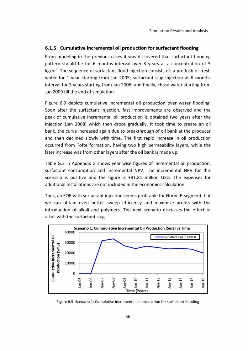
56
Simulation Results and Analysis
6.1.5 Cumulative incremental oil production for surfactant flooding
From modeling in the previous cases it was discovered that surfactant flooding
pattern should be for 6 months interval over 3 years at a concentration of 5
kg/m3. The sequence of surfactant flood injection consists of: a preflush of fresh
water for 1 year starting from Jan 2005; surfactant slug injection at 6 months
interval for 3 years starting from Jan 2006; and finally, chase water starting from
Jan 2009 till the end of simulation.
Figure 6.9 depicts cumulative incremental oil production over water flooding.
Soon after the surfactant injection, fast improvements are observed and the
peak of cumulative incremental oil production is obtained two years after the
injection (Jan 2008) which then drops gradually. It took time to create an oil
bank, the curve increased again due to breakthrough of oil bank at the producer
and then declined slowly with time. The first rapid increase in oil production
occurred from Tofte formation, having two high permeability layers, while the
later increase was from other layers after the oil bank is made up.
Table G.2 in Appendix G shows year wise figures of incremental oil production,
surfactant consumption and incremental NPV. The incremental NPV for this
scenario is positive and the figure is +91.81 million USD. The expenses for
additional installations are not included in the economics calculation.
Thus, an EOR with surfactant injection seems profitable for Norne E-segment, but
we can obtain even better sweep efficiency and maximize profits with the
introduction of alkali and polymers. The next scenario discusses the effect of
alkali with the surfactant slug.
Figure 6.9: Scenario 1: Cumulative incremental oil production for surfactant flooding
0
10000
20000
30000
40000
Jan
-05
Jan
-06
Jan
-07
Jan
-08
Jan
-09
Jan
-10
Jan
-11
Jan
-12
Jan
-13
Jan
-14
Jan
-15
Jan
-16Cu
mu
lati
ve In
cre
me
nta
l Oil
Pro
du
ctio
n (
Sm3
)
Time (Years)
Scenario 1: Cummulative Incremental Oil Production (Sm3) vs Time
Surfactant Slug (5 kg/m3)

57
Simulation Results and Analysis
6.2 Scenario 2: Alkaline-Surfactant (AS) Flooding
The synergistic effect of alkaline and surfactant results in less surfactant required
to recover significant incremental oil. In the Alkaline Surfactant (AS) process, a
very low concentration of the surfactant is used to achieve ultra low interfacial
tension between the trapped oil and the injection fluid/formation water. The
ultra low interfacial tension also allows the alkali present in the injection fluid to
infiltrate deeply into the formation and contact the trapped oil globules. The
alkali then reacts with the acidic components in the crude oil to form additional
surfactant in-situ, thus, continuously providing ultra low interfacial tension and
freeing the trapped oil. The addition of alkali increases pH, alters rock wettability
(from oil-wet to water-wet) and lowers the surfactant adsorption so that very
low surfactants can be used to reduce cost (34).
In the previous scenario, the surfactant of 5kg/m3 concentration was used and
even with this concentration the incremental NPV was positive. The surfactant is
relatively expensive and to reduce its consumption, alkali was injected with low
concentration surfactant slug to produce in situ surfactant. The sequence of
Alkaline-surfactant flood injection consists of: a preflush of fresh water for 1 year
starting from Jan 2005; Alkaline-surfactant slug injection at 6 months interval for
3 years starting from Jan 2006; and finally, chase water starting from Jan 2009 till
the end of simulation.
Following three cases were simulated at a constant concentration of alkali (2
kg/m3) and with different concentrations of surfactant.
6.2.1 AS flooding at concentrations of 2 kg/m3 and 0.3 kg/m3 respectively
6.2.2 AS flooding at concentrations of 2 kg/m3 and 2 kg/m3 respectively
6.2.3 AS flooding at concentrations of 2 kg/m3 and 5 kg/m3 respectively
In Figure 6.10, the cumulative incremental oil production is almost same for all
surfactant concentrations (0.3 kg/m3, 2 kg/m3 & 5 kg/m3). The alkali is performing
well in reducing the residual oil saturation by generating additional in-situ
surfactant, thus reducing surfactant consumption.
Since, the incremental oil production at the 5 kg/m3 surfactant concentration is
same as with 0.3 kg/m3 concentration, so it is rather wasteful to inject 5 kg/m3

58
Simulation Results and Analysis
surfactant (Figure 6.11) and also this concentration yields high surfactant at the
producer (Figure 6.12). Figure 6.13 shows reservoir pressure of alkaline-
surfactant flooding which is maintained below the constrain (300 bara) and
above the bubble point (251 bara).
Table G.3, Table G.4, and Table G.5 shows year wise figures of incremental oil
production and incremental NPVs for different surfactant concentrations. The
incremental NPV of 0.3 kg/m3 surfactant concentration is +98.74 million USD
which is higher than the NPV of other concentrations (2 kg/m3 & 5 kg/m3) and
also scenario 1.
Thus in terms of incremental NPV, the surfactant of concentration 0.3 kg/m3 is
the right choice for this scenario and also alkali-surfactant flooding (scenario 2) is
yielding more net cash flows than surfactant flooding (scenario 1).
Figure 6.10: Scenario 2: Cumulative incremental oil production for alkaline-surfactant flooding
0
10000
20000
30000
40000
Jan
-05
Jan
-06
Jan
-07
Jan
-08
Jan
-09
Jan
-10
Jan
-11
Jan
-12
Jan
-13
Jan
-14
Jan
-15
Jan
-16
Cu
mu
lati
ve In
crem
enta
l Oil
Pro
du
ctio
n (
Sm3
)
Time (Years)
Scenario 2: Cummulative Incremental Oil Production (Sm3) vs Time
ALK-SUR Slug (2kg/m3 & 0.3kg/m3)
ALK-SUR Slug (2kg/m3 & 2kg/m3)
ALK-SUR Slug (2kg/m3 & 5kg/m3)

59
Simulation Results and Analysis
Figure 6.11: Scenario 2: Total alkaline-surfactant injection for different surfactant concentrations
Figure 6.12: Scenario 2: Surfactant production rate for different concentrations
Figure 6.13: Scenario 2: Reservoir pressure for alkaline-surfactant flooding

60
Simulation Results and Analysis
6.3 Scenario 3: Polymer Flooding
Polymer flooding is one of the chemical EOR techniques and can yield a
significant increase in oil recovery compared to conventional water flooding
technique. Unlike surfactant, polymer does not reduce the interfacial tension
between water and oil but it improves volumetric sweep efficiency by increasing
water viscosity. This increase in viscosity lowers mobility ratio, decreases the
chances of fingering, and allows more oil to be contacted on a macroscopic scale.
Typical polymer injection sequence is described as: a preflush usually consisting
of a low- salinity brine or fresh water to condition the reservoir; the polymer
solution itself for mobility control to minimize channeling; and finally, chase or
drive water to move the polymer solution and resulting oil bank to the
production wells (22). The flow of polymer solution through the porous medium is
assumed to have no influence on the flow of the hydrocarbon phases.
The objective of this scenario is to know the incremental NPV based on
incremental oil production if this EOR technique is to be applied to Norne E-
segment. The sequence of polymer flood injection for this scenario consists of: a
preflush of fresh water for 1 year starting from Jan 2005; continuous polymer
injection for 3 years starting from Jan 2006; and finally, chase water starting from
Jan 2009 till the end of simulation.
The following three cases were simulated to identify which concentration of
polymer would generate high incremental NPV.
6.3.1 Polymer flooding at concentration of 0.5 kg/m3
6.3.2 Polymer flooding at concentration of 0.7 kg/m3
6.3.3 Polymer flooding at concentration of 1.0 kg/m3
Figure 6.14 proves the classical theory about the effect of polymer flooding on
water production rate. The trends from this figure are that the higher the
polymer concentration, the lower the water production rate, and faster the
water production increase. It can be seen from Figure 6.15 of Buckley Leverett
that the water saturation is high behind the trailing edge for a polymer flooding
than a water flooding. When this more even polymer flood front breaks through,
more water will be produced at the same time as in our case (Figure 6.14). It has
been clearly seen that the polymer concentration played an important role in

61
Simulation Results and Analysis
sweep efficiency; polymer of concentration 1.0 kg/m3 has less water production
and much better volumetric sweep efficiency than the water flooding case. The
water front moves faster through the reservoir in the water flooding case.
The cumulative incremental oil production for three different concentrations is
shown in Figure 6.16. The polymer of concentration 1.0 kg/m3 would have high
incremental oil production because of high viscosity. Although, high
concentration improves mobility ratio and displacement efficiency but also have
more chances of polymer adsorption, retention, and entrapment. The peak oil
production for all cases is achieved in 2010 and after 2013 the oil production
became lower than water flooding. This is because due to good volumetric
sweep efficiency, the more oil was produced before the breakthrough of front
and after breakthrough low oil production is due to less oil saturation left behind.
Figure 6.17 shows the reservoir pressure of polymer flooding which is maintained
above the bubble point (251 bara) and below the maximum constrain (300 bara).
Table G.6, Table G.7, and Table G.8 shows year wise figures of incremental oil
production and cumulative incremental NPVs for different polymer
concentrations. The incremental NPV of 1.0 kg/m3 polymer concentration is
+56.83 million USD which is higher than the NPV of other concentrations (0.5
kg/m3 & 0.7 kg/m3). However, the incremental NPV of this scenario is lower than
scenario 1 and scenario 2.
Thus, in terms of incremental NPV, the polymer of concentration 1.0 kg/m3 is
most favorable choice for this scenario.
Figure 6.14: Scenario 3: Water Production rate for polymer flooding

62
Simulation Results and Analysis
Figure 6.15: Buckley Leverett solution for polymer flooding compared to water flooding (35)
Figure 6.16: Scenario 3: Cumulative incremental oil production for polymer flooding
Figure 6.17: Scenario 3: Reservoir pressure for polymer flooding
-10000
0
10000
20000
30000
40000
50000
60000
70000
Jan
-05
Jan
-06
Jan
-07
Jan
-08
Jan
-09
Jan
-10
Jan
-11
Jan
-12
Jan
-13
Jan
-14
Jan
-15
Jan
-16
Cu
mm
ula
tive
Incr
emen
tal O
il P
rod
uct
ion
(Sm
3)
Time (Years)
Scenario 3: Cummulative Incremental Oil Production (Sm3) vs Time
Polymer Concentration (0.5 kg/m3)Polymer Concentration (0.7 kg/m3)Polymer Concentration (1.0 kg/m3)

63
Simulation Results and Analysis
6.4 Scenario 4: Surfactant-Polymer (SP) Flooding
In the Surfactant Polymer (SP) Flood process, a very low concentration of low
adsorption surfactant is used to achieve ultra low interfacial tension between the
trapped oil and the injection fluid/formation water while polymer acts as
viscosity modifier and helps mobilize the oil. Often, the SP slug is followed by
polymer “push” solution to improve volumetric sweep efficiency, reduce
channeling and breakthrough and they can also provide mobility control at the
low IFT front. Otherwise, the front is not stable and will finger and dissipate.
Upon the completion of polymer injection, driving fluid (water) is injected to
move the chemicals and resulting oil bank towards production wells. Generally,
the reservoir is conditioned by preflush (with fresh water, alkali or polymer
depending on rock mineralogy) before the injection of SP slug into reservoir (30).
For this scenario, the sequence of SP flood injection consists of: a preflush of
fresh water for 1 year starting from Jan 2005; surfactant or SP slug injection for 3
years (6 months interval) starting from Jan 2006; and finally, chase water starting
from Jan 2009 till the end of simulation.
The following two cases were simulated to discover which method generates
higher incremental NPV.
6.4.1 Surfactant slug (5 kg/m3) followed by polymer (0.4 kg/m3)
6.4.2 SP slug (5 kg/m3 & 0.4 kg/m3) followed by polymer (0.4 kg/m3)
Figure 6.18 shows the cumulative incremental oil production for above two
cases. Soon after the surfactant/SP slug injection, the fast improvements were
observed and the first peak of cumulative oil production was obtained two years
after the injection (Jan 2008) which then drops gradually. Second highest peak
was observed in Jan 2012 which was due to breakthrough of oil bank at the
producer. The first peak of oil production occurred from the two high
permeability layers (Tofte formation), while second peak of oil production
resulted from other layers after the oil bank was made up.
The case 6.4.2 has higher incremental oil production than case 6.4.1 (Figure 6.18,
Table G.9 and Table G.10 ) and also comparatively low water production (Figure
6.19). This is because of the presence of polymer in the surfactant slug. As
discussed in scenario 3, the polymer increases the viscosity of the formulation,

64
Simulation Results and Analysis
resulting in favorable mobility ratio, less chance of fingering, and allows more oil
to be contacted on a macroscopic scale.
As can be seen in Table G.9 and Table G.10, the incremental NPV for case 6.4.2 is
higher than case 6.4.1. Also, this NPV (+117.49 Million USD) is higher than
scenario 1, scenario 2 and scenario 3.
Thus, in terms of incremental NPV, the case 6.4.2 is the optimal choice for this
scenario.
Figure 6.18: Scenario 4: Cumulative incremental oil production for surfactant-polymer flooding
Figure 6.19: Scenario 4: Water production total for surfactant-polymer flooding
0
10000
20000
30000
40000
50000
60000
Jan
-05
Jan
-06
Jan
-07
Jan
-08
Jan
-09
Jan
-10
Jan
-11
Jan
-12
Jan
-13
Jan
-14
Jan
-15
Jan
-16
Cu
mm
ula
tive
Incr
emen
tal O
il P
rod
uct
ion
(S
m3
)
Time (Years)
Scenario 4: Cummulative Incremental Oil Production (Sm3) vs Time
Surfactant Slug followed by Polymer
SP Slug followed by Polymer

65
Simulation Results and Analysis
6.5 Scenario 5: Alkaline-Surfactant-Polymer (ASP) Flooding
The sequence of ASP flood injection for this scenario consists of: preflush of fresh
water for 1 year starting from Jan 2005; injection of ASP slug for 3 years (6
months interval) starting from Jan 2006; and finally, chase water starting from
Jan 2009 till the end of simulation.
The following two cases were simulated.
6.5.1 ASP slug (2 kg/m3, 0.3 kg/m3 & 0.4 kg/m3) followed by polymer (0.4
kg/m3)
6.5.2 Desorption / no desorption of surfactant and polymer
Figure 6.20 shows the cumulative incremental oil production for ASP flooding.
The incremental oil production trend of this scenario is almost matching (little
difference) with Figure 6.18 of scenario 4 (case 6.4.2). Compared to previous
scenario, the additional chemical in this scenario is Alkaline which is relatively
cheap and its addition can reduce the expenses of surfactant. The surfactant
concentration is reduced from 5 kg/m3 to 0.3 kg/m3 while polymer concentration
is same. The alkali is performing well in reducing the residual oil saturation by
generating additional in-situ surfactant. As shown in Figure 6.21, the reservoir
pressure profile is maintained above the bubble point pressure (251 bara) and
below the maximum constrain (300 bara).
The cumulative incremental oil production given in Table G.11 is 4530 Sm3 less
than scenario 4 (case 6.4.2) while the incremental NPV of ASP flooding (+123.50
million USD) is higher than SP flooding (case 6.4.2) and also all scenarios.
Figure 6.22 shows that maximum of 1.40 % oil recovery factor is achieved from
ASP flooding (55.70%) compared to water flooding (54.30 %).
In all scenarios, desorption of chemicals was prevented as per my assumption.
Figure 6.23 and Figure 6.24 shows the effect of desorption/no desorption of
surfactant and polymer respectively. The adsorption of chemicals on rock
surfaces is an instantaneous effect. Desorption refers to decrease of chemicals
adsorbed on rock surfaces with time. We can see in both figures that when
desorption model is active, the adsorbed chemicals in the block decreased as the
time passes, which is due to presence of alkali and also continued exposure to

66
Simulation Results and Analysis
water flood. If desorption is prevented then the adsorbed chemicals may not
decrease with time. Practically, desorption of chemicals may not be as efficient
as in this case.
Thus, in terms of high incremental NPV, less surfactant/polymer adsorption
effect, and less water production, ASP flooding can be the potential EOR method
for Norne E-segment.
Figure 6.20: Scenario 5: Cumulative incremental oil production for ASP flooding
Figure 6.21: Scenario 5: Reservoir pressure for ASP flooding
0
10000
20000
30000
40000
50000
60000
Jan
-05
Jan
-06
Jan
-07
Jan
-08
Jan
-09
Jan
-10
Jan
-11
Jan
-12
Jan
-13
Jan
-14
Jan
-15
Cu
mm
ula
tive
Incr
emen
tal O
il P
rod
uct
ion
(S
m3
)
Time (Years)
Scenario 5: Cummulative Incremental Oil Production (Sm3) vs Time
ASP Slug followed by Polymer

67
Simulation Results and Analysis
Figure 6.22: Scenario 5: Oil recovery factor for ASP flooding
Figure 6.23: Scenario 5: Effect of desorption or no desorption of surfactant in block (7, 57, 9)
Figure 6.24: Scenario 5: Effect of desorption or no desorption of polymer in block (7, 57, 9)

68
Simulation Results and Analysis
6.6 Comparison between Incremental NPV for all Scenarios
As described in section 5.5, the Net Present Value (NPV) criterion was selected in
order to determine the most appropriate chemical EOR method for the Norne E-
segment. The NPV calculation is based on incremental oil production from
chemical flooding (alkaline, surfactant, and/or polymer) compared to water
flooding.
The tables in Appendix G for all scenarios present the NPV calculation based on
incremental oil production. Figure 6.25 shows the incremental NPV for all
scenarios. The incremental NPV of ASP flooding (Scenario 5) is higher than all of
the scenarios. Both Scenario 2 (AS flood) and Scenario 5 (ASP flood) has same
alkaline (2 kg/m3) and surfactant (0.3 kg/m3) concentrations; the additional
product in Scenario 5 is polymer. The polymer characteristics to improve
volumetric sweep efficiency by decreasing the mobility ratio resulted in increase
in cumulative incremental oil production; ultimately net present value became
high.
The surfactant concentration (5 kg/m3) in both Scenario 4 (SP flood) and Scenario
1 (Surfactant flood) is equal; the improvement in incremental NPV for Scenario 4
is due to polymer in the slug and also mobility control behind of the slug.
The incremental oil as well NPV for Scenario 3 (polymer flood) are lower than all
of the scenarios. This is because, unlike surfactant, polymer does not release the
capillary trapped oil but it improves volumetric sweep efficiency and reduces
mobility ratio by increasing water viscosity. Ultimately, our goal to reduce
residual oil saturation may not be achieved. Polymer enhances the efficiency of
the AS flood when pumped with and behind the slug as observed in scenario 5.
Keeping in view the above and previous discussion in scenarios, it is concluded
that ASP flooding (scenario 5) can be applied to Norne E-segment to release
capillary trapped oil from Ile and Tofte formations. The maximum of 1.40 %
incremental recovery factor and incremental NPV of +123.53 million USD were
achieved with ASP flooding.

69
Simulation Results and Analysis
Figure 6.25: Incremental NPV for all scenarios
-20
0
20
40
60
80
100
120
140
Incr
em
en
tal N
et
Pre
sern
t V
alu
e, M
illio
n U
SD
Time (Years)
Comparision between Incremental NPV for all Scenarios
Scenario 1 (Surfactant Flooding)
Scenario 2 (Alkali-Surfactant Flooding)
Scenario 3 (Polymer Flooding)
Scenario 4 (SP Flooding)
Scenario 5 (ASP Flooding)

70
Simulation Results and Analysis
6.7 Single Parameter Sensitivity Analysis (Spider Plot) for ASP
Flooding
Sensitivity analysis measures the impact on project outcomes of changing one or
more key input values about which there is uncertainty. Spider plot is one of the
standard tools used in risk and uncertainty analysis. Spider diagram is a graph
that compares the potential impact, taking one input at a time, of several
uncertain input variables on project outcomes.
The uncertain parameters for this project are oil price, discount rate, and
chemical prices (alkaline, surfactant and polymer). The sensitivity analysis is done
on the basis of base case sheet by varying a single parameter while keeping all
the base case parameters constant (Table G.12 in appendix G). The NPVs (based
on discount rate and prices of oil, alkaline, surfactant, and polymer) for high case,
base case and low case extracted from Table G.12 are presented in Table 6.1,
where sensitivity is done in terms of % change.
From Figure 6.26, it can be seen that in case of increase in oil price (+55.56%), %
change NPV is +58.26%; whereas for low case, the % change NPV is -58.31% with
% change oil price (-55.56%). This means that change in oil price has huge effect
on NPV.
Equally rise of prices of alkali, polymer and surfactant (50%), % change NPV with
% change polymer price is +1.15% comparison with % change surfactant price
and alkali price is +0.20% and 0.68% respectively. It means that change in
polymer price has slight high effect on NPV than change in surfactant and alkali
price.
Percentage change in discount rate (+25% and -25%) has also great effect on NPV
(+9.29% & -8.12%) respectively but less than oil price.
From above analysis it is obvious that change in oil price has substantial effect on
NPV compared to other parameters while surfactant price is the least sensitive
parameter i.e very low affect on NPV for high/low case.

71
Simulation Results and Analysis
Table 6.1: Single parameter sensitivity analysis
Low Base High
Oil Price (U$/bbl) 40 90 140 % Change -55.56% 0% 55.56% NPV (Million NOK) 51.50 123.53 195.50
% Change -58.31% 0% 58.26%
Alkaline Price (kg/m3) 0.75 1.50 2.25
% Change -50.00% 0% 50.00% NPV (Million NOK) 122.69 123.53 124.37 % Change -0.68% 0% 0.68%
Polymer Price (kg/m3) 2.00 4.00 6.00 % Change -50.00% 0% 50.00%
NPV (Million NOK) 122.11 123.53 124.95
% Change -1.15% 0% 1.15%
Surfactant Price (kg/m3) 1.75 3.50 5.25
% Change -50.0% 0% 50.0% NPV (Million NOK) 123.28 123.53 123.78 % Change -0.20% 0% 0.20%
Discount Rate 0.10 0.08 0.06 % Change 25.0% 0% -25.0% NPV (Million NOK) 113.50 123.53 135.00
% Change -8.12% 0% 9.29%
Figure 6.26: Single parameter sensitivity analysis (Spider Plot) for Scenario 5
-50%-40%-30%-20%-10%
0%
10%20%
30%40%
50%
-50% -30% -10% 10% 30% 50% 70%
% C
han
ge N
PV
% Change Variable
Scenario 5 (ASP Flooding): SPIDER (Sensitivity Diagram)
Oil PriceAlkaline PricePolymer PriceSurfactant PriceDiscount Rate

72
Discussion and Summary
7 Discussion and Summary
The EOR screening criteria suggested by Taber et al. (1) was applied to Norne E-
segment in order to come up with right EOR method that would reduce residual
oil saturation. Five EOR scenarios such as surfactant flooding, alkaline-surfactant
flooding, polymer flooding, surfactant-polymer and ASP were simulated for the
Norne E-segment. After comparative study, ASP flooding was concluded as a
possible EOR method for the Norne E-segment.
Before simulating these scenarios, the injector and producer for EOR study were
selected. The surfactant injection in well F3-H gave comparatively little higher
recovery factor with less surfactant consumption than injection in F-1H or F-1H &
F-3H. This is because F-1H is located in water zone; the injected surfactant will
spread out instead of attacking the residual oil. Also, surfactant has to travel for
long before it can start to mobilize capillary trapped oil and a lot of surfactant is
required due to adsorption/retention. The well E-2H was selected as a producer
because of its location in our main target formations.
The scenario 1 was about surfactant flooding. A series of simulation cases were
done in order to know the right quantity of surfactant that would yield maximum
recovery of residual trapped oil. An attempt was made to compare continuous
injection with slug injection. The injection of surfactant in slug form at 6 months
interval (for 3 years) instead of continuous injection (for 3 or 6 years) was
chosen. The incremental oil recovery for 3 or 6 years continuous injection
compared to 3 years slug injection was not encouraging and it was rather
wasteful to inject surfactant in former case. Also, slug injection has less effects of
surfactant adsorption than continuous. The surfactant slug injection during 3
years involves injecting surfactant for one month after every 6 months interval
followed by water. Injecting surfactant of higher concentration (10 kg/m3, 15
kg/m3 and 30 kg/m3) did not prove to be profitable than 5 kg/m3 concentration,
because of no significant difference in cumulative oil production.
Having established the most effective surfactant flooding method, one case was
simulated to calculate the incremental NPV for scenario 1. The drop in
cumulative incremental oil production after some years with production can be
explained by a poorer sweep efficiency achieved with the use of surfactant. Due
to heterogeneous nature of the reservoir, the breakthrough of the surfactant will
first occur in the layers of high permeability causing the decrease of residual oil

73
Discussion and Summary
saturation in theses layers and there is expected that relative permeability to
water has increased, simply because the water is trapped by less oil. Thus, low
permeability layers will be attacked less by the surfactant. Many researchers
have validated these findings through their experiments. For our case, the first
rapid increase in oil production occurred from Tofte formation, having two high
permeability layers, while the later increase was from other layers of Ile and
Tofte after the oil bank was made up.
For scenario 2, the addition of alkali (2 kg/m3) in low concentration surfactant
slug resulted in almost similar cumulative incremental oil production but higher
incremental NPV than scenario 1. Alkali performed well in reducing the residual
oil saturation by generating additional in-situ surfactant, resulting in less
surfactant required. Surfactant concentration of 0.3 kg/m3 for this scenario
generated higher NPV than other concentrations (2 kg/m3 and 5 kg/m3). The
trend of incremental oil production curve is similar to scenario 1.
The scenario 3 is about polymer flooding. Unlike surfactant, polymer is not able
to reduce the interfacial tension between water and oil but it improves
volumetric sweep efficiency by increasing water viscosity. This classical theory
was proved in our case, where high incremental oil production with less water
production was obtained compared to water flooding. The peak of oil production
was achieved in 2010 and after 2013 the oil production became lower than water
flooding. This is because due to good volumetric sweep efficiency (piston like),
the more oil was produced before the breakthrough of front and after
breakthrough low oil production was due to less oil saturation left behind. This
behavior is matching with Figure 6.15 of Buckley Leverett solution. The polymer
of concentration 1.0 kg/m3 had high incremental oil production because of high
viscosity as well high incremental NPV than other concentrations (0.5 kg/m3 and
0.7 kg/m3). The low NPV of this scenario compared to scenario 1 and scenario 2 is
because polymer injection alone cannot release capillary trapped oil. Instead,
polymer with alkaline and/or surfactant would yield high recovery.
The scenario 4 is about surfactant-polymer flooding. The addition of mobility
control (polymer) in Scenario 1 (surfactant slug) resulted in high incremental
recovery due to good volumetric sweep efficiency. ‘SP slug followed by polymer’
gave more incremental oil production as well NPV than ‘surfactant slug followed
by polymer’. This is because polymer in the surfactant slug due to its high
viscosity makes favorable mobility ratio and also reduces the chances of

74
Discussion and Summary
fingering, resulting in high incremental oil production. The NPV of this scenario is
comparatively higher than scenario 1, scenario 2 and scenario 3.
In scenario 5, the synergistic effect of alkaline, surfactant and polymer (ASP)
resulted in less surfactant required to recover significant incremental oil. As
mentioned in scenario 2 and scenario 4 that alkali makes the project profitable
by creating the natural soap in-situ (if total acid number (TAN) is high), reducing
the expenses of surfactant while polymer acts as viscosity modifier and helps
mobilize the oil. Having above qualities, the highest NPV was achieved for ASP
flooding (scenario 5) than other scenarios. The 1.40% incremental recovery
factor by ASP flooding would generate a net present value of +123.53 million
USD.
The desorption effect was restricted in all scenarios. When a case of ASP was run
with active desorption model, the adsorbed surfactant and polymer in the block
decreased with time. This is due to presence of alkali and also continued
exposure to water flood. If desorption is prevented then the adsorbed chemicals
may not decrease with time.
In the end, single price sensitivity (Spider plot) at different oil prices, chemicals
prices, and discount rate for low case, base case, and high case was also
performed. It was found that change in oil price has substantial effect on NPV
compared to other parameters while surfactant price is the least sensitive
parameter i.e very low affect on NPV for high/low case.
Thus, in terms of high incremental NPV among all scenarios, the ASP flooding
seems an attractive EOR method for Norne E-segment especially when the Ile
and Tofte formations are targeted. The success of this method depends on the
identification of the proper alkali, surfactant, and polymer and on the way they
are combined to produce compatible formulation that yields good crude oil
emulsification / mobilization, low chemical losses and good mobility control (29).
The operational and additional facilities costs; and oil and chemicals prices also
play important roles in the success of an EOR project which are not included in
the economics calculation. In addition, the chemical properties (alkali, surfactant
and polymer) used in this study are not actually related to Norne E-segment and
practically may or may not be compatible with Norne reservoir and fluid
characteristics; because no laboratory research regarding this chemical EOR
method has been performed yet.

75
Conclusion and Recommendation
8 Conclusion and Recommendation
8.1 Conclusion
The ASP flooding is a good candidate for an EOR project at Norne E-segment
and should be injected earlier.
The ASP flooding can increase the incremental recovery factor of 1.40% in the
target formations (Ile & Tofte)
The injector F-3H will be more viable candidate for ASP flooding than F-1H.
The producer E-2H will be better candidate for ASP flooding because of its
location in our main target formations.
The injection of S/AS/SP/ASP in slug form at 6 months interval (for 3 years)
was economically viable than continuous injection (for 3 or 6 years).
Surfactant concentration of 5 kg/m3 gave same oil production with less
surfactant consumption compared to 10 kg/m3, 15 kg/m3 and 30 kg/m3.
Polymer concentration of 1 kg/m3 gave higher cumulative incremental NPV
compared to 0.5 kg/m3 and 0.7 kg/m3.
It was found from single parameter sensitivity analysis (Spider plot) that
change in oil price (for low case, base case, and high case) has considerable
effect on NPV compared to discount rate, alkali price, surfactant price and
polymer price.
Surfactant price is the least sensitive parameter i.e very low affect on NPV for
high/low case.
8.2 Recommendation
It is recommended that right alkali, surfactant and polymer structure that would
be compatible with fluid and rock properties of Norne field E-segment, be
developed in the laboratory. It is also important that up-scaling the appropriate
laboratory identified chemicals to a field-scale usage be done correctly. The
timing of ASP injection into Norne E-segment is also recommended to be early in
the life of the field because injection of ASP at a later time might not lead to best
possible oil recovery. The addition of co-surfactants and co-solvents in the ASP
solution could also be tried out to see if it would make the flooding more
effective.

76
<Bibliography
Bibliography
1. Taber, J.J, Martin, F.D and Seright, R.S. EOR Screening Criteria Revisited-Part1:
Introduction to Screening Criteria and Enhanced Recovery Field Projects, SPE
Reservoir Engineering. August 1997. 12(3):189-198.
2. Sheng, James J. Modern Chemical Enhanced Oil Recovery (Theory and
Practice), Elsevier Inc, USA. 2011.
3. Donnelly, John. Global Demand Surge, JPT Editor. August 2011.
4. Awan, A.R and Reigland, R. and Kleppe, J. A Survey of North Sea Enhanced-Oil-
Recovery Projects Initiated during the Years 1975 to 2005, SPE 99546. April 2006.
5. Norwegian Petroleum Directorate (NPD). Improved Recovery without Side
Effects (http://www.npd.no/en/Topics/Improved-
Recovery/Temaartikler/Improved-recovery-without-side-effects/) accessed on
August 8, 2011.
6. Cheng, Nan. Principal Engineer, Reservoir Technology at Statoil, Rotvoll
Trondheim Norway (contacted on August 11, 2011).
7. Emegwalu, Chinenye Clara. Thesis-Enhanced Oil Recovery for Norne Field's E-
Segment using Surfactant Flooding. 2010.
8. Kalnaes, Per Einar. Thesis-An EOR Evaluation of Surfactant Flooding in the
Norne E-Segment based on Applied Reservoir Simulation. June 2010.
9. Awolola, Kazeem, Bjornar, Mariann and Asphaug, Engeset and Sarkar,
Summe. The Potential for Surfactant Flooding in the Norne E-segment, Experts in
Team (Norne Village). March 2011.
10. Sundt, Tine, et al. Comparative Study of Different EOR Methods for Norne E-
segment, Experts in Team (Norne Village). May, 2011.
11. Chierici, Gian Luigi. Principle of Petroleum Reservoir Engineering, volume 2,
Springer-Verlag. 1995.
12. Schmidt, R.L. Thermal Enhanced Oil Recovery—Current Status and Future
Needs. January 1990.

77
<Bibliography
13. Ali, S.M.Farouq and Thomas, S. A Realistic Look at Enhanced Oil Recovery,
Scientia Iranica, Vol. 1, No. 3, Sharif University of Technology. October 1994.
14. Statoil (2004). Annual Reservoir Development Plan, Norne Field.
15. IO-Center (2011). Welcome to IO Center-Norne Benchmark Case, Introduction
to Norne Field,
(http://www.ipt.ntnu.no/~norne/wiki/data/media/english/gfi/introduction-to-
the-norne-field.pdf), accessed on July 7, 2011.
16. Statoil (2001). PL 128 Norne, Reservoir Management Plan.
17. NPD (2010). The NPD's fact-pages. [Online]
(http://www.npd.no/engelsk/cwi/pbl/en/field/all/43778.htm), accessed on July
8, 2011.
18. Statoil (1994). PDO-Reservoir Geology, Support Documentation.
19. Statoil (2006). Annual Reservoir Development Plan, Norne and Urd Field.
20. Statoil (1994). PL 128 Plan for Development and Operation Support
Document-Reservoir Engineering. June 1994.
21. Green, D.W and Willhite, G.P. Enhanced Oil Recovery-SPE Text-book Series
vol 6, Society of Petroleum Engineers, Richardson Texas. 1998.
22. Lake, Larry W. Enhanced Oil Recovery, University of Texas at Austin. 1989.
23. Akstinat, M.H. Surfactants for EOR Process in High-Salinity System: Product
Selection and Evaluation, F.J Fayers(ed.) New York, Elsevier. 1981.
24. Kleppe, Jon and Skjaeveland, Svein. M. SPOR Monograph-Recent Advances
in Improved Oil Recovery Methods for North Sea Sandstone Reservoirs, NPD
Stavanger. 1992.
25. Liu, Shunhua. Alkaline Surfactant Polymer Enhanced Oil Recovery Process,
Phd Thesis, Rice University Houstan Texas. Januray, 2008.
26. FLOPAAM™. Polymers for Enhanced Oil Recovery from design to injection
(http://www.snf-group.com/IMG/pdf/Oil_EOR-FLOPAAM-Desert.pdf) accessed
on July 22, 2011 . [Online]

78
27. Petroleum Development Oman. Polymer Flooding
(http://www.pdo.co.om/pdoweb/tabid/278/Default.aspx), accesed on July 22,
2011. [Online]
28. S.Majidaie, Tan, Isa M. and Demiral, Birol M.R. Review of ASP Flooding,
Universitti Teknologi PETRONAS, Malaysia.
29. Al-Hashim, H.S., et al. Alkaline Surfactant Polymer Formulation for Carbonate
Reservoirs, Petroleum Science and Technology, 23:723-746,2005. May 5, 2004.
30. TIORCO. ASP/ASP Technologies (http://www.tiorco.com/pdf/cutsheet/ASP-
SP_cutsheet.pdf), accessed on July 26, 2011.
31. United Energy Group (UEG) . Enhanced Oil Recovery Presentation,
(www.unitedenergy.com/pdf/2008_03_EOR_Enhanced_Oil_Recovery.pdf)
accessed on July 26, 2011.
32. Schlumberger. Eclipse Technical Description Manual . 2009.2.
33. Investopedia. Net Present Value
(http://www.investopedia.com/terms/n/npv.asp) accessed on July 27, 2011.
34. Oil Chem Technologies. ENHANCED OIL RECOVERY, (http://www.oil-
chem.com/asp.htm), accessed on July 31, 2011.
35. Nguyen, Long Hai. Master's Thesis, Reservoir Simulation for IOR with Polymer
Flooding in Norwegian Field, NTNU. June 2008.
36. Oil Chem Technologies, Inc. Cost of chemicals (www.oil-chem.com), accessed
on July 10, 2011.

79
APPENDICES

80
APPENDICES
A. The Surfactant Model in Eclipse
A.1 Calculation of the Capillary Number
The capillary number is a dimensionless ratio of viscous forces to capillary forces (32).
(A. 1)
where
K = permeability
P = potential
ST = interfacial tension
Cunit = conversion factor depending on the unit used
is calculated as
(A. 2)
where for cell i
(A. 3)
and similarly for the y and z directions.
A.2 Relative Permeability Model
The Relative Permeability model is very important in Eclipse and is a transition
from immiscible relative permeability curves at low capillary number to miscible
relative permeability curves at high capillary number. The user supplies a table
that describes the transition as a function of log10 (capillary number).
The procedure to calculate oil to water relative permeability curve is illustrated in
Figure A. 1. Firstly the end points of the curve are interpolated (point A) and both
the immiscible and the miscible curves are scaled between A and B. The relative
permeability values are looked up on both curves, and the final relative
permeability is taken as an interpolation between these two values (32).

81
APPENDICES
Figure A. 1 Calculation of relative permeability (32)
A.3 Capillary Pressure
Capillary pressure is the difference in pressure across the interface between two
immiscible fluids and is defined as
(A. 4)
The water oil capillary pressure will reduce as the concentration of surfactant
increases and actually it is the reduction in the water oil capillary pressure that
reduces the residual oil saturation (32). The oil water capillary pressure is given as:
(A. 5)
where
= surface tension at the present surfactant concentration
= surface tension at zero concentration
= capillary pressure from the immiscible curves initially scaled to the interpolated end points calculated in the relative permeability model.
A.4 Water PVT Properties
The surfactant modifies the viscosity of the pure or salted water input using the
PVTW or PVTWSALT keyword respectively. The SURFVISC keyword is used to
represent the surfactant viscosity as a function of surfactant concentration and is

82
APPENDICES
used to calculate the water-surfactant solution viscosity as shown in equation A.6 (32).
(A. 6)
where
= surfactant viscosity
= water viscosity
= viscosity of the water-surfactant mixture.
= reference pressure in the PVTW or PVTWSALT keywords.
= reference salt concentration
A.5 Adsorption
The adsorption of surfactant is assumed to be immediate, and the quantity
adsorbed is a function of the surrounding surfactant concentration and is given
by (32):
(A. 7)
Where
= Pore volume of the cell
MD = mass density of the rock
= adsorption isotherm as a function of local surfactant concentration
in solution
A.6 Keywords for Surfactant Flood Model in Eclipse 100
The model is activated by specifying the keyword SURFACT in the RUNSPEC
section. In the PROPS section three keywords (SURFVISC, SURFST and SURFCAPD)
and one in the Schedule section (WSURFACT) are obligatory while two optional
keywords could be used for cases in which adsorption takes place. Table A.1
gives a summary of the surfactant keywords and their descriptions (32).

83
APPENDICES
Table A.1: Surfactant Model Keywords (32)
Keyword Description Notes
SURFACT Activates Surfactant model and keyword has no associated data
Obligatory
SURFST Water-oil Surface tension in the presence of surfactant
Obligatory
SURFVISC Modified water viscosity Obligatory
SURFCAPD Capillary de-saturation data Obligatory
SURFROCK Rock properties and adsorption model indicator
If SURFADS is present
SURFNUM For specifying miscible relative permeability curves
SURFADS Adsorption isotherm Optional
WSURFACT Injected surfactant concentration of water injector
Obligatory

84
APPENDICES
B The Polymer Flood Model in Eclipse
B.1 Material Balance for Polymer Flooding
The standard black-oil equations used to describe the hydrocarbon phases in the
model are as follows:
Water:
(B. 1)
Polymer:
(B. 2)
Brine:
(B. 3)
(B. 4)
where
= dead pore space within each grid cell
= polymer adsorption concentration
= mass density of the rock formation
= relative permeability reduction factor for the aqueous phase due to polymer retention
= polymer and salt concentrations respectively in the aqueous phase
= effective viscosity of the water (a=w), polymer (a=p) and salt (a=s).
= cell center depth.
= transmissibility
= block pore volume
= water production rate
The model assumes that the density and formation volume factor of the aqueous
phase are independent of the polymer and salt concentrations. The polymer
solution, reservoir brine and the injected water are represented in the model as
miscible components in the aqueous phase, where the degree of mixing is
specified through the viscosity terms in the conservation equations (32).

85
APPENDICES
B.2 Treatment of Fluid Viscosities
The viscosity terms used in the fluid flow equations contain the effects of a
change in the viscosity of the aqueous phase due to the presence of polymer and
salt in the solution.
To get the effective polymer viscosity, it is required to enter the viscosity of a
fully mixed polymer solution as an increasing function of the polymer
concentration in solution . The effective polymer viscosity is calculated
as follows:
(B. 5)
where
= Todd-Longstaff mixing parameter
The mixing parameter is useful in modeling the degree of segregation between
the water and the injected polymer solution. If ω = 1 then the polymer solution
and water are fully mixed in each block. If ω = 0 the polymer solution is
completely segregated from the water (32).
B.3 Treatment of Polymer Adsorption
Adsorption is treated as an instantaneous effect in the model. The effect of
polymer adsorption is to create a stripped water bank at the leading edge of the
slug. Desorption effects may occur as the slug passes.
There are two adsorption models, either can be selected. The first model ensures
that each grid block retraces the adsorption isotherm as the alkaline
concentration rises and falls in the cell. The second model assumes that if
desorption is prevented then the adsorbed polymer concentration may not
decrease with time, and hence does not allow for any desorption (32).
B.4 Treatment of Permeability Reductions and Dead Pore Volume
The adsorption process causes a reduction in the permeability of the rock to the
passage of the aqueous phase and is directly correlated to the adsorbed polymer
concentration. In order to compute the reduction in rock permeability, it is
required to specify the residual resistance factor (RRF) for each rock type. The
actual resistance factor can be calculated as:

86
APPENDICES
(B. 6)
The value of the maximum adsorbed concentration, , depends on the rock
type and needs to be specified by the user. This value must be non zero. The user
should also specify the dead pore volume for each rock type. It represents the
amount of total pore volume in each grid cell that is inaccessible to the polymer
solution (32).
B.5 Treatment of Shear Thinning Effect
The shear thinning of polymer has the effect of reducing the polymer viscosity at
higher flow rates. Eclipse assumes that shear rate is proportional to the flow
viscosity. This assumption is not valid in general, as for example, a given flow in a
low permeability rock will have to pass through smaller pore throats than the
same flow in a high permeability rock, and consequently the shear rate will be
higher in the low permeability rock. However for a single reservoir this
assumption is probably reasonable (32).
The reduction in the polymer viscosity is assumed to be reversible as a function
of the water velocity and is calculated as:
(B. 7)
where
= shear viscosity of the polymer solution (water + polymer)
= effective water viscosity
= viscosity multiplier assuming no shear effect
= shear thinning multiplier
= 1 represents no shear thinning, whereas = 0 shows maximum shear thinning
B.6 Keywords for Polymer Flood Model in Eclipse 100
The model is activated by the keyword POLYMER in the RUNSPEC section. The
mixing parameter data is obligatory and should be defined using the keyword
TLMIXPAR. The maximum number of mixing parameter regions is set using the
parameter NTMISC in the keyword MISCIBLE. The maximum polymer and salt
concentrations to be used in calculating the effective fluid component viscosities

87
APPENDICES
are entered under the keyword PLYMAX. The viscosity of a fully mixed polymer
solution is defined by the keyword PLYVISC.
The polymer adsorption data should be entered using the keyword PLYADS in the
PROPS section. Other polymer-rock parameters such as the rock mass density
used in the adsorption calculation, the dead pore volume and the residual
resistance factor are input using the keyword PLYROCK. The shear thinning
model is activated if the PLYSHEAR keyword is present in the PROPS section. The
shear thinning data consists of tables of viscosity reduction as a function of local
velocity. The concentration of the injected polymer in water injector is specified
using the WPOLYMER keyword in the SCHEDULE section (32).
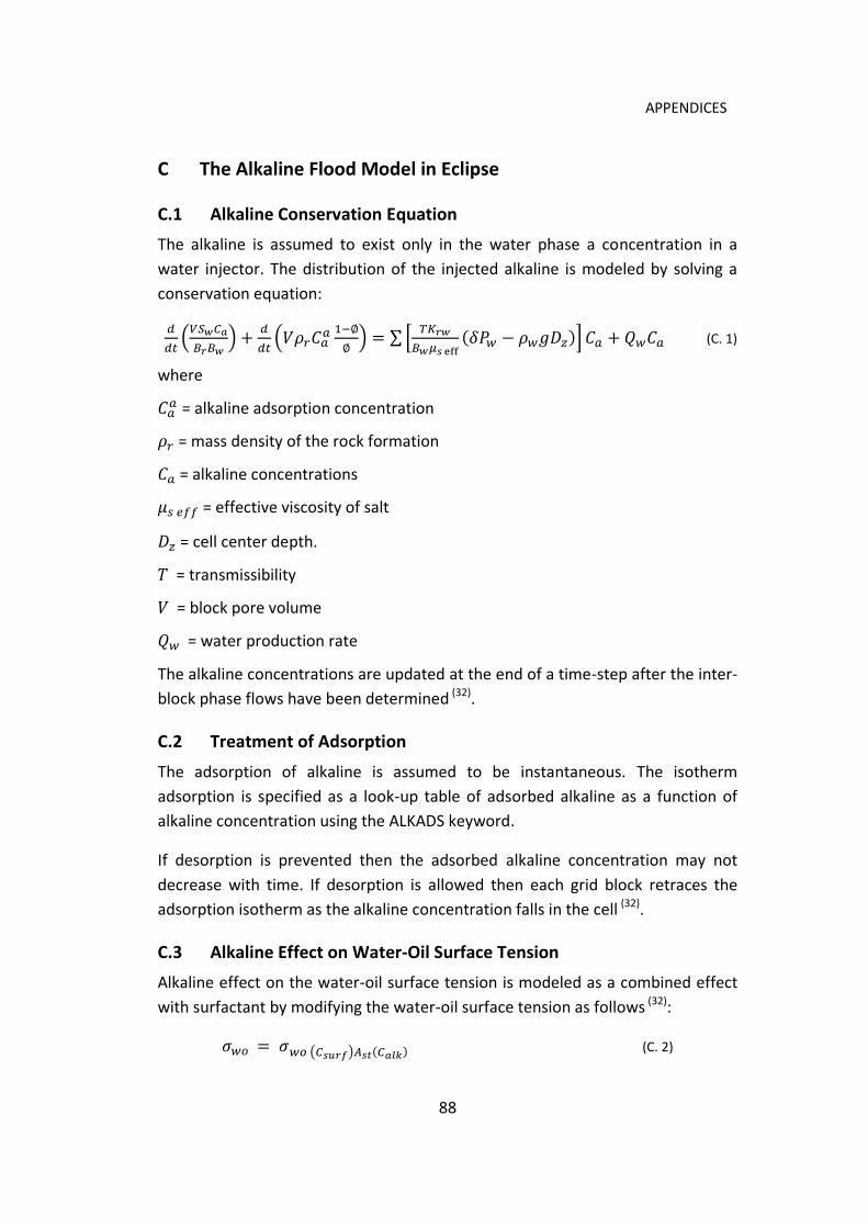
88
APPENDICES
C The Alkaline Flood Model in Eclipse
C.1 Alkaline Conservation Equation
The alkaline is assumed to exist only in the water phase a concentration in a
water injector. The distribution of the injected alkaline is modeled by solving a
conservation equation:
(C. 1)
where
= alkaline adsorption concentration
= mass density of the rock formation
= alkaline concentrations
= effective viscosity of salt
= cell center depth.
= transmissibility
= block pore volume
= water production rate
The alkaline concentrations are updated at the end of a time-step after the inter-
block phase flows have been determined (32).
C.2 Treatment of Adsorption
The adsorption of alkaline is assumed to be instantaneous. The isotherm
adsorption is specified as a look-up table of adsorbed alkaline as a function of
alkaline concentration using the ALKADS keyword.
If desorption is prevented then the adsorbed alkaline concentration may not
decrease with time. If desorption is allowed then each grid block retraces the
adsorption isotherm as the alkaline concentration falls in the cell (32).
C.3 Alkaline Effect on Water-Oil Surface Tension
Alkaline effect on the water-oil surface tension is modeled as a combined effect
with surfactant by modifying the water-oil surface tension as follows (32):
(C. 2)

89
APPENDICES
= surface tension at surfactant concentration and zero alkaline
concentration
= surface tension multiplier at alkaline concentration
C.4 Alkaline Effect on Surfactant/Polymer Adsorption
The alkaline can reduce the adsorption of both surfactant and polymer on the
rock surface. This is modeled by modifying the mass of adsorbed surfactant or
polymer as follows (32):
(C. 3)
where
= pore volume of the cell
= surfactant/polymer adsorbed concentration
= adsorption multiplier at alkaline concentration
C.5 Keywords for Polymer Flood Model in Eclipse 100
This model is activated by specifying the ALKALINE keyword in the RUNSPEC
section. The Polymer Flood Model or the Surfactant Flood Model should be
active as well. Table C.1 gives a summary of the alkaline model keywords and
their descriptions (32).
Table C.1: Alkaline Model Keywords
Keyword Description Notes
ALKALINE Activates Alkaline model and keyword has no associated data
Obligatory
ALSURFST Table of oil/water surface tension as a function of alkaline concentration
Obligatory if the Surfactant Flood Model is active
ALSURFAD Table of surfactant adsorption as a function of alkaline concentration
Obligatory if the SURFADS keyword is used
ALPOLADS Table of Polymer adsorption as a function of alkaline concentration
Obligatory if the Polymer Flood Model is active
ALKADS Table of adsorption functions Optional
ALKROCK Specifies alkaline-rock adsorption/desorption properties
Obligatory if ALKADS is used
WSURFACT Specifies the concentration of the injected alkaline in a water injector
Obligatory
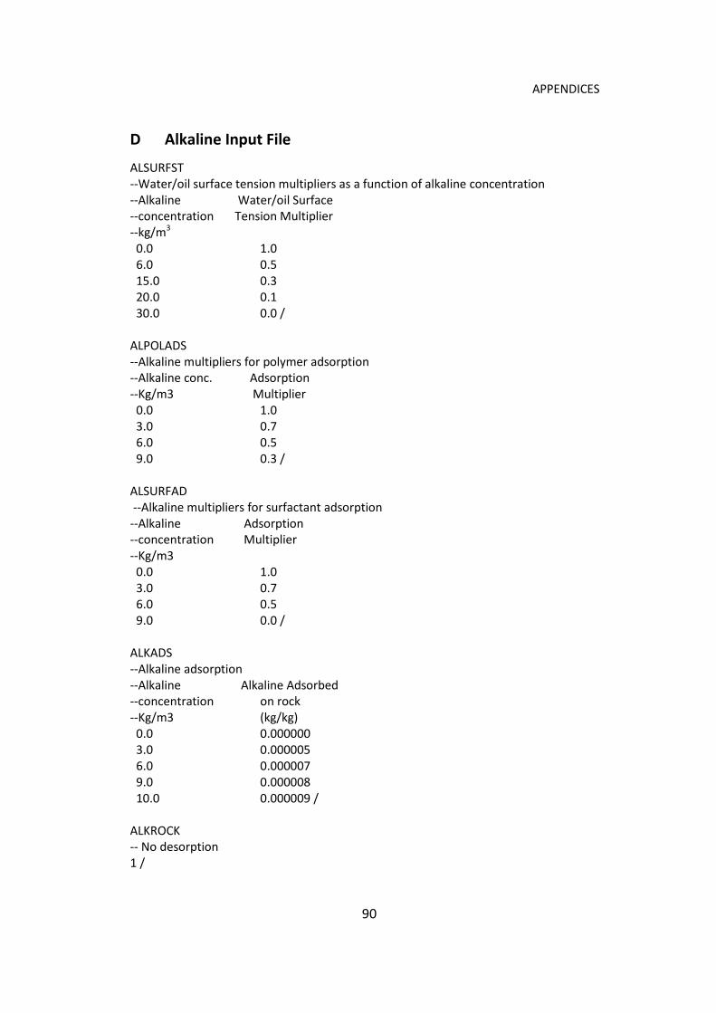
90
APPENDICES
D Alkaline Input File
ALSURFST --Water/oil surface tension multipliers as a function of alkaline concentration --Alkaline Water/oil Surface --concentration Tension Multiplier --kg/m3 0.0 1.0 6.0 0.5 15.0 0.3 20.0 0.1 30.0 0.0 / ALPOLADS --Alkaline multipliers for polymer adsorption --Alkaline conc. Adsorption --Kg/m3 Multiplier 0.0 1.0 3.0 0.7 6.0 0.5 9.0 0.3 / ALSURFAD --Alkaline multipliers for surfactant adsorption --Alkaline Adsorption --concentration Multiplier --Kg/m3 0.0 1.0 3.0 0.7 6.0 0.5 9.0 0.0 / ALKADS --Alkaline adsorption --Alkaline Alkaline Adsorbed --concentration on rock --Kg/m3 (kg/kg) 0.0 0.000000 3.0 0.000005 6.0 0.000007 9.0 0.000008 10.0 0.000009 / ALKROCK -- No desorption 1 /

91
APPENDICES
E Surfactant Input File
SURFST -- Surfactant Water/oil Surface --conc., kg/m3 Tension, N/m 0 30.0E-03 0.1 10.0E-03 0.25 1.60E-03 0.5 0.40E-03 1.0 0.07E-03 3.0 0.006E-03 5.0 0.004E-03 10.0 0.006E-03 20.0 0.01E-03 /
SURFVISC --Surf conc Water Viscosity --Kg/m3 Centipoise 0.0 0.42 5.0 0.449 10.0 0.503 15.0 0.540 20.0 0.630 /
SURFADS --Surfactant Adsorption by rock --Surf conc Adsorbed mass --Kg/m3 (kg/kg) = kg surf /kg rock 0.0 0.00000 1.0 0.00017 5.0 0.00017 10.0 0.00017 /
SURFCAPD --Capillary De-saturation curve --Log10 (capillary Miscibility --number) function 0 = immiscible, 1= miscible -8 0.0 -7 0.0 -6 0.0 -5.0 0.0 -2.5 1.0 0 1.0 5 1.0 10 1.0/ SURFROCK -- No desorption 1 2650/

92
APPENDICES
F Polymer Input File
PLYSHEAR --Polymer shear thinning data -- Wat. Velocity Visc reduction -- m/day CP 0.0 1.0 2.0 1.0 / PLYVISC -- Polymer solution Viscosity Function -- Ply conc. Wat. Visc. mult. -- kg/m3 0.0 1.0 0.1 1.55 0.3 2.55 0.5 5.125 0.7 8.125 1.0 21.2 / PLYADS -- Polymer Adsorption Function -- Ply conc. Ply conc. Adsorbed -- kg/m3 by rock, Kg/kg 0.0 0.0 0.5 0.0000017 1.0 0.0000017 / TLMIXPAR -- Todd-Long staff Mixing Parameters 1 1* / PLYMAX -- Polymer-Salt concentration for mixing maximum polymer and salt concentration -- Ply conc. Salt conc. -- kg/m3 kg/m3 1.0 0.0 / PLYROCK --Polymer-Rock Properties --dead pore residual resistance mass Ads. max. Polymer -- space factor density Index adsorption 0.16 1.0 2650 1 0.000017 /

93
APPENDICES
Discount Factor 0.08
Oil Price USD/bbl 90
Alkaline Price USD/kg 1.50 Polymer Price USD/kg 4.00 Surfactant Price USD/kg 3.50 Color code Red: Input
Table G.2: Scenario 1: Incremental NPV for Surfactant Slug (5kg/m3) Injection for 3 years (6 months interval)
Time
Annual Oil Production
Annual Annual Present
Value (PV) NPV
Base Case
With Surfactant
Oil Increment
Surfactant Consumption
Year Year Sm3 Sm3 Sm3 bbl kg Million USD Million USD
2005 0 701,610 701,610 0 0 0 0.00 0.00
2006 1 565,280 597,110 31,830 200,204 1,085,000 13.17 13.17
2007 2 465,850 499,440 33,590 211,274 1,085,000 13.05 26.21
2008 3 388,310 415,270 26,960 169,573 1,085,000 9.10 35.31
2009 4 332,590 356,830 24,240 152,465 0 10.09 45.40
2010 5 291,440 318,040 26,600 167,309 0 10.25 55.65
2011 6 254,430 279,490 25,060 157,622 0 8.94 64.59
2012 7 232,890 256,730 23,840 149,949 0 7.87 72.46
2013 8 211,040 235,440 24,400 153,471 0 7.46 79.92
2014 9 191,500 215,090 23,590 148,376 0 6.68 86.61
2015 10 160,900 180,760 19,860 124,915 0 5.21 91.81
The NPV for Scenario 1 91.81

94
APPENDICES
Table G.3: Scenario 2 (6.2.1): Incremental NPV for Alkaline-Surfactant Slug (2kg/m3 & 0.3kg/m3) Injection for 3 years (6 months interval)
Time
Annual Oil Production
Annual Annual Annual
Present Value (PV)
NPV Base Case
With Alkaline-
Surfactant OilIncrement
Alkaline Consumption
Surfactant Consumption
Year Year Sm3 Sm3 Sm3 bbl kg kg Million USD Million
USD
2005 0 701,610 701,610 0 0 0 0 0.00 0.00
2006 1 565,280 597,080 31,800 200,016 434,000 65,100 15.85 15.85
2007 2 465,850 499,160 33,310 209,513 434,000 65,100 15.41 31.27
2008 3 388,310 414,930 26,620 167,434 434,000 65,100 11.26 42.53
2009 4 332,590 356,490 23,900 150,326 0 0 9.94 52.48
2010 5 291,440 317,980 26,540 166,931 0 0 10.22 62.70
2011 6 254,430 279,390 24,960 156,993 0 0 8.90 71.60
2012 7 232,890 256,580 23,690 149,005 0 0 7.82 79.43
2013 8 211,040 235,290 24,250 152,528 0 0 7.42 86.85
2014 9 191,500 215,070 23,570 148,251 0 0 6.67 93.52
2015 10 160,900 180,820 19,920 125,293 0 0 5.22 98.74
The NPV for Scenario 2 (6.2.1) 98.74

95
APPENDICES
Table G.4: Scenario 2 (6.2.2): Incremental NPV for Alkaline-Surfactant Slug (2kg/m3 & 2kg/m3) Injection for 3 years (6 months interval)
Time
Annual Oil Production
Annual Annual Annual
Present Value (PV)
NPV Base Case
With Alkaline-
Surfactant
Oil Increment
Alkaline Consumption
Surfactant Consumption
Year Year Sm3 Sm3 Sm3 bbl kg kg Million USD Million
USD
2005 0 701,610 701,610 0 0 0 0 0.00 0.00
2006 1 565,280 597,090 31,810 200,079 434,000 434,000 14.66 14.66
2007 2 465,850 499,160 33,310 209,513 434,000 434,000 14.31 28.97
2008 3 388,310 415,000 26,690 167,875 434,000 434,000 10.27 39.24
2009 4 332,590 356,590 24,000 150,955 0 0 9.99 49.23
2010 5 291,440 317,950 26,510 166,743 0 0 10.21 59.44
2011 6 254,430 279,400 24,970 157,056 0 0 8.91 68.35
2012 7 232,890 256,620 23,730 149,257 0 0 7.84 76.19
2013 8 211,040 235,360 24,320 152,968 0 0 7.44 83.62
2014 9 191,500 215,070 23,570 148,251 0 0 6.67 90.30
2015 10 160,900 180,770 19,870 124,978 0 0 5.21 95.51
The NPV for Scenario 2 (6.2.2) 95.51

96
APPENDICES
Table G.5: Scenario 2 (6.2.3): Incremental NPV for Alkaline-Surfactant Slug (2kg/m3 & 5kg/m3) Injection for 3 years (6 months interval)
Time
Annual Oil Production
Annual Annual Annual
Present Value (PV)
NPV Base Case
With Alkaline-
Surfactant
Oil Increment
Alkaline Consumption
Surfactant Consumption
Year Year Sm3 Sm3 Sm3 bbl kg kg Million USD Million
USD
2005 0 701,610 701,610 0 0 0 0 0.00 0.00
2006 1 565,280 597,150 31,870 200,456 434,000 1,085,000 12.59 12.59
2007 2 465,850 499,470 33,620 211,463 434,000 1,085,000 12.50 25.09
2008 3 388,310 415,300 26,990 169,762 434,000 1,085,000 8.60 33.69
2009 4 332,590 356,850 24,260 152,591 0 0 10.09 43.78
2010 5 291,440 318,030 26,590 167,246 0 0 10.24 54.02
2011 6 254,430 279,490 25,060 157,622 0 0 8.94 62.96
2012 7 232,890 256,700 23,810 149,760 0 0 7.86 70.83
2013 8 211,040 235,420 24,380 153,345 0 0 7.46 78.28
2014 9 191,500 215,080 23,580 148,313 0 0 6.68 84.96
2015 10 160,900 180,760 19,860 124,915 0 0 5.21 90.17
The NPV for Scenario 2 (6.2.3) 90.17

97
APPENDICES
Table G.6: Scenario 3 (6.3.1): Incremental NPV for Continuous Polymer Injection (0.5kg/m3)
Time
Annual Oil Production
Annual Annual Present
Value (PV) NPV
Base Case
With Polymer
Oil Increment
Polymer Consumption
Year Year Sm3 Sm3 Sm3 bbl kg Million USD Million USD
2005 0 701,610 701,610 0 0 0 0.00 0.00
2006 1 565,280 569,600 4,320 27,172 638,750 -0.10 -0.10
2007 2 465,850 491,290 25,440 160,013 638,750 10.16 10.05
2008 3 388,310 418,830 30,520 191,965 640,500 11.68 21.74
2009 4 332,590 366,820 34,230 215,300 0 14.24 35.98
2010 5 291,440 307,550 16,110 101,329 0 6.21 42.19
2011 6 254,430 259,280 4,850 30,506 0 1.73 43.92
2012 7 232,890 232,310 -580 -3,648 0 -0.19 43.72
2013 8 211,040 207,400 -3,640 -22,895 0 -1.11 42.61
2014 9 191,500 186,160 -5,340 -33,588 0 -1.51 41.10
2015 10 160,900 155,190 -5,710 -35,915 0 -1.50 39.60
The NPV for Scenario 3 (6.3.1) 39.60

98
APPENDICES
Table G.7: Scenario 3 (6.3.2): Incremental NPV for Continuous Polymer Injection (0.7kg/m3)
Time
Annual Oil Production
Annual Annual Present
Value (PV) NPV
Base Case
With Polymer
Oil Increment
Polymer Consumption
Year Year Sm3 Sm3 Sm3 bbl kg Million USD Million USD
2005 0 701,610 701,610 0 0 0 0.00 0.00
2006 1 565,280 568,810 3,530 22,203 894,250 -1.46 -1.46
2007 2 465,850 495,630 29,780 187,310 894,250 11.39 9.92
2008 3 388,310 425,790 37,480 235,742 896,700 14.00 23.92
2009 4 332,590 376,240 43,650 274,550 0 18.16 42.08
2010 5 291,440 312,210 20,770 130,639 0 8.00 50.08
2011 6 254,430 261,750 7,320 46,041 0 2.61 52.70
2012 7 232,890 232,630 -260 -1,635 0 -0.09 52.61
2013 8 211,040 207,050 -3,990 -25,096 0 -1.22 51.39
2014 9 191,500 185,460 -6,040 -37,990 0 -1.71 49.68
2015 10 160,900 154,300 -6,600 -41,513 0 -1.73 47.95
The NPV for Scenario 3 (6.3.2) 47.95

99
APPENDICES
Table G.8: Scenario 3 (6.3.3): Incremental NPV for Continuous Polymer Injection (1.0 kg/m3)
Time
Annual Oil Production
Annual Annual Present
Value (PV) NPV
Base Case
With Polymer
Oil Increment
Polymer Consumption
Year Year Sm3 Sm3 Sm3 bbl kg Million USD Million USD
2005 0 701,610 701,610 0 0 0 0.00 0.00
2006 1 565,280 566,390 1,110 6,982 1,277,500 -4.15 -4.15
2007 2 465,850 498,260 32,410 203,852 1,277,500 11.35 7.20
2008 3 388,310 432,810 44,500 279,896 1,281,000 15.93 23.13
2009 4 332,590 390,370 57,780 363,425 0 24.04 47.17
2010 5 291,440 320,670 29,230 183,851 0 11.26 58.43
2011 6 254,430 265,190 10,760 67,678 0 3.84 62.27
2012 7 232,890 232,830 -60 -377 0 -0.02 62.25
2013 8 211,040 206,190 -4,850 -30,506 0 -1.48 60.77
2014 9 191,500 184,530 -6,970 -43,840 0 -1.97 58.79
2015 10 160,900 153,400 -7,500 -47,174 0 -1.97 56.83
The NPV for Scenario 3 (6.3.3) 56.83

100
APPENDICES
Table G.9: Scenario 4 (6.4.1): Incremental NPV for Surfactant Slug (5kg/m3) Injection for 3 years (6 months interval) followed by Polymer ( 0.40 kg/m3) for 2 years and chase water
Time
Annual Oil Production
Annual Annual Annual
Present Value (PV)
NPV Base Case
With Polymer-
Surfactant
Oil Increment
Polymer Consumption
Surfactant Consumption
Year Year Sm3 Sm3 Sm3 bbl kg kg Million USD Million
USD
2005 0 701,610 701,610 0 0 0 0 0.00 0.00
2006 1 565,280 597,190 31,910 200,708 0 1,085,000 13.21 13.21
2007 2 465,850 499,480 33,630 211,526 0 1,085,000 13.07 26.28
2008 3 388,310 415,270 26,960 169,573 0 1,085,000 9.10 35.38
2009 4 332,590 357,920 25,330 159,321 511,000 0 9.04 44.41
2010 5 291,440 334,490 43,050 270,776 511,000 0 15.19 59.61
2011 6 254,430 303,840 49,410 310,779 0 0 17.63 77.23
2012 7 232,890 270,250 37,360 234,987 0 0 12.34 89.57
2013 8 211,040 242,680 31,640 199,009 0 0 9.68 99.25
2014 9 191,500 217,340 25,840 162,528 0 0 7.32 106.57
2015 10 160,900 179,710 18,810 118,311 0 0 4.93 111.50
The NPV for Scenario 4 (6.4.1) 111.50

101
APPENDICES
Table G.10: Scenario 4 (6.4.2): Incremental NPV for Surfactant-Polymer Slug (5kg/m3) Injection for 3 years (6 months interval) followed by Polymer ( 0.40 kg/m3) for 2 years and chase water
Time
Annual Oil Production
Annual Annual Annual
Present Value (PV)
NPV Base Case
With Polymer-
Surfactant
Oil Increment
Polymer Consumption
Surfactant Consumption
Year Year Sm3 Sm3 Sm3 bbl kg kg Million USD Million
USD
2005 0 701,610 701,610 0 0 0 0 0.00 0.00
2006 1 565,280 599,430 34,150 214,797 86,800 1,085,000 14.06 14.06
2007 2 465,850 503,330 37,480 235,742 86,800 1,085,000 14.64 28.70
2008 3 388,310 419,820 31,510 198,192 86,800 1,085,000 10.87 39.57
2009 4 332,590 362,430 29,840 187,688 511,000 0 10.91 50.48
2010 5 291,440 336,940 45,500 286,186 511,000 0 16.14 66.62
2011 6 254,430 304,320 49,890 313,798 0 0 17.80 84.42
2012 7 232,890 269,800 36,910 232,157 0 0 12.19 96.61
2013 8 211,040 241,540 30,500 191,839 0 0 9.33 105.94
2014 9 191,500 215,970 24,470 153,911 0 0 6.93 112.87
2015 10 160,900 178,530 17,630 110,889 0 0 4.62 117.49
The NPV for Scenario 4 (6.4.2) 117.49

102
APPENDICES
Table G.11: Scenario 5 (6.5.1): Incremental NPV for ASP (2kg/m3, 0.3kg/m3 & 0.4kg/m3) Injection for 3 years (6 months interval) followed by Polymer (0.40kg/m3) injection for 2 years and Chase Water
Time
Annual Oil Production
Annual Annual Annual Annual Present Value (PV)
NPV Base Case
With ASP Oil
Increment Alkaline
Consumption Surfactant
Consumption Polymer
Consumption
Year Year Sm3 Sm3 Sm3 bbl kg kg kg Million
USD Million
USD
2005 0 701,610 701,610 0 0 0 0 0 0.00 0.00
2006 1 565,280 599,390 34,110 214,545 434,000 65,100 86,800 16.74 16.74
2007 2 465,850 503,220 37,370 235,050 434,000 65,100 86,800 17.09 33.83
2008 3 388,310 419,590 31,280 196,745 434,000 65,100 86,800 13.08 46.91
2009 4 332,590 362,110 29,520 185,675 0 0 511,000 10.78 57.69
2010 5 291,440 336,720 45,280 284,802 0 0 511,000 16.05 73.75
2011 6 254,430 303,890 49,460 311,094 0 0 0 17.64 91.39
2012 7 232,890 269,150 36,260 228,068 0 0 0 11.98 103.37
2013 8 211,040 240,680 29,640 186,430 0 0 0 9.06 112.43
2014 9 191,500 215,130 23,630 148,628 0 0 0 6.69 119.12
2015 10 160,900 177,700 16,800 105,669 0 0 0 4.41 123.53
The NPV for Scenario 5 (6.5.1) 123.53

103
APPENDICES
Table G.12: Single parameter sensitivity analysis for low case, base case, and high case at different oil prices, chemicals prices, and discount rate
Change in discount rate
Change in oil price Change in alkaline
price Change in polymer
price Change in Surfactant
price
Low Base High Low Base High Low Base High Low Base High Low Base High
Discount Factor 0.10 0.08 0.06 0.08 0.08 0.08 0.08 0.08 0.08 0.08 0.08 0.08 0.08 0.08 0.08
Oil Price USD/bbl 90 90 90 40 90 140 90 90 90 90 90 90 90 90 90
Alk. Price USD/kg 1.50 1.50 1.50 1.50 1.50 1.50 2.25 1.50 0.75 1.50 1.50 1.50 1.50 1.50 1.50
Poly. Price USD/kg 4.00 4.00 4.00 4.00 4.00 4.00 4.00 4.00 4.00 5.50 4.00 2.50 4.00 4.00 4.00
Surf. Price USD/kg 3.50 3.50 3.50 3.50 3.50 3.50 3.50 3.50 3.50 3.50 3.50 3.50 5.00 3.50 2.00
Year Year Present Value (PV), Million USD
2005 0 0.0 0.0 0.0 0.0 0.0 0.0 0.0 0.0 0.0 0.0 0.0 0.0 0.0 0.0 0.0
2006 1 16.4 16.7 17.1 6.8 16.7 26.7 16.4 16.7 17.0 16.6 16.7 16.9 16.7 16.7 16.8
2007 2 16.5 17.1 17.7 7.0 17.1 27.2 16.8 17.1 17.4 17.0 17.1 17.2 17.0 17.1 17.2
2008 3 12.4 13.1 13.8 5.3 13.1 20.9 12.8 13.1 13.3 13.0 13.1 13.2 13.0 13.1 13.2
2009 4 10.0 10.8 11.6 4.0 10.8 17.6 10.8 10.8 10.8 10.2 10.8 11.3 10.8 10.8 10.8
2010 5 14.6 16.1 17.6 6.4 16.1 25.7 16.1 16.1 16.1 15.5 16.1 16.6 16.1 16.1 16.1
2011 6 15.8 17.6 19.7 7.8 17.6 27.4 17.6 17.6 17.6 17.6 17.6 17.6 17.6 17.6 17.6
2012 7 10.5 12.0 13.7 5.3 12.0 18.6 12.0 12.0 12.0 12.0 12.0 12.0 12.0 12.0 12.0
2013 8 7.8 9.1 10.5 4.0 9.1 14.1 9.1 9.1 9.1 9.1 9.1 9.1 9.1 9.1 9.1
2014 9 5.7 6.7 7.9 3.0 6.7 10.4 6.7 6.7 6.7 6.7 6.7 6.7 6.7 6.7 6.7
2015 10 3.7 4.4 5.3 2.0 4.4 6.9 4.4 4.4 4.4 4.4 4.4 4.4 4.4 4.4 4.4
NPV, Million USD 113.5 123.5 135.0 51.5 123.5 195.5 122.7 123.5 124.4 122.1 123.5 124.9 123.3 123.5 123.8

104
Prediction Input File
Prediction Input File DATES 1 'JAN' 2005 / / COMPDAT -- WELL I J K1 K2 Sat. CF DIAM KH SKIN ND DIR Ro 'F-3H' 7 57 5 5 'OPEN' 1* 3.427 0.216 328.264 2* 'Z' 18.296 / 'F-3H' 7 57 6 6 'OPEN' 1* 3.391 0.216 325.229 2* 'Z' 18.420 / 'F-3H' 7 57 7 7 'OPEN' 1* 4.284 0.216 410.644 2* 'Z' 18.352 / 'F-3H' 7 57 8 8 'OPEN' 1* 4.241 0.216 407.082 2* 'Z' 18.498 / 'F-3H' 7 57 9 9 'OPEN' 1* 9.387 0.216 902.750 2* 'Z' 18.667 / 'F-3H' 7 57 10 10 'OPEN' 1* 101.082 0.216 9741.795 2* 'Z' 18.876 / 'F-3H' 7 57 11 11 'OPEN' 1* 4.716 0.216 454.519 2* 'Z' 18.880 / 'F-3H' 7 57 12 12 'OPEN' 1* 1.659 0.216 160.153 2* 'Z' 19.011 / 'F-3H' 7 57 13 13 'OPEN' 1* 123.532 0.216 11909.055 2* 'Z' 18.905 / 'F-3H' 7 57 14 14 'OPEN' 1* 23.785 0.216 2299.001 2* 'Z' 19.163 / 'F-3H' 7 57 15 15 'OPEN' 1* 9.266 0.216 897.482 2* 'Z' 19.375 / 'F-3H' 7 56 15 15 'OPEN' 1* 2.873 0.216 278.581 2* 'Z' 19.470 / 'F-3H' 7 56 16 16 'OPEN' 1* 213.422 0.216 20730.869 2* 'Z' 19.660 / 'F-3H' 7 56 17 17 'OPEN' 1* 22.442 0.216 2174.958 2* 'Z' 19.427 / 'F-3H' 7 56 18 18 'OPEN' 1* 22.435 0.216 2194.387 2* 'Z' 20.384 / 'F-3H' 7 56 19 19 'OPEN' 1* 16.226 0.216 1590.031 2* 'Z' 20.581 / 'F-3H' 7 56 20 20 'OPEN' 1* 85.791 0.216 8439.256 2* 'Z' 21.005 / 'F-3H' 7 56 21 21 'OPEN' 1* 42.255 0.216 4130.474 2* 'Z' 20.320 / 'F-3H' 7 56 22 22 'OPEN' 1* 300.194 0.216 29777.980 2* 'Z' 21.955 / / WCONPROD 'E-2H' 'OPEN' 'BHP' 5* 235 / / WSURFACT 'F-3H' 0.0 / / WPOLYMER 'F-3H' 0.0 0.0 / / WALKALIN 'F-3H' 0 / / WCONINJE 'C-1H' 'WATER' 1* 'RATE' 10121.652 1* 450 3* / 'C-2H' 'WATER' 1* 'RATE' 9064.145 1* 450 3* / 'C-3H' 'GAS' 'SHUT' 'RATE' 1627788.907 1* 600 3* / 'C-4AH' 'WATER' 'OPEN' 'RATE' 4303.281 1* 450 3* / --F-1H injection rate tuned down from 10,000 m3/d to 7000 m3/d 'F-1H' 'WATER' 'OPEN' 'RATE' 7000 1* 450 3* / 'F-2H' 'WATER' 1* 'RATE' 5846.826 1* 450 3* / 'F-3H' 'WATER' 'OPEN' 'RATE' 3500 1* 450 3* / 'F-4H' 'WATER' 'OPEN' 'RATE' 1555.877 1* 450 3* /

105
Prediction Input File
/ RPTSCHED 'FIP=2' 'WELLS=2' 'SUMMARY=2' ALKALINE/ 'SURFBLK' 'SURFADS' 'PLYADS' 'PBLK' / ------------------------------------------------------- DATES 1 'JAN' 2006 / / WSURFACT 'F-3H' 0.3 / / WPOLYMER 'F-3H' 0.40 0.0 / / WALKALIN 'F-3H' 5 / / RPTSCHED 'FIP=2' 'WELLS=2' 'SUMMARY=2' ALKALINE/ 'SURFBLK' 'SURFADS' 'PLYADS' 'PBLK' / ------------------------------------------------------- DATES 1 'FEB' 2006 / / WSURFACT 'F-3H' 0.0 / / WPOLYMER 'F-3H' 0.0 0.0 / / WALKALIN 'F-3H' 0 / / RPTSCHED 'FIP=2' 'WELLS=2' 'SUMMARY=2' ALKALINE/ 'SURFBLK' 'SURFADS' 'PLYADS' 'PBLK' / ------------------------------------------------------- DATES 1 'AUG' 2006 / / WSURFACT 'F-3H' 0.3 / / WPOLYMER 'F-3H' 0.40 0.0 / / WALKALIN 'F-3H' 5 / / RPTSCHED 'FIP=2' 'WELLS=2' 'SUMMARY=2' ALKALINE/ 'SURFBLK' 'SURFADS' 'PLYADS' 'PBLK' / -------------------------------------------------------

106
Prediction Input File
DATES 1 'SEP' 2006 / / WSURFACT 'F-3H' 0.0 / / WPOLYMER 'F-3H' 0.00 0.0 / / WALKALIN 'F-3H' 0 / / RPTSCHED 'FIP=2' 'WELLS=2' 'SUMMARY=2' ALKALINE/ 'SURFBLK' 'SURFADS' 'PLYADS' 'PBLK' / DATES 1 'MAR' 2007 / / WSURFACT 'F-3H' 0.3 / / WPOLYMER 'F-3H' 0.40 0.0 / / WALKALIN 'F-3H' 5 / / RPTSCHED 'FIP=2' 'WELLS=2' 'SUMMARY=2' ALKALINE/ 'SURFBLK' 'SURFADS' 'PLYADS' 'PBLK' / ------------------------------------------------------- DATES 1 'APR' 2007 / / WSURFACT 'F-3H' 0.0 / / WPOLYMER 'F-3H' 0.0 0.0 / / WALKALIN 'F-3H' 0 / / RPTSCHED 'FIP=2' 'WELLS=2' 'SUMMARY=2' ALKALINE/ 'SURFBLK' 'SURFADS' 'PLYADS' 'PBLK' / ------------------------------------------------------- DATES 1 'OCT' 2007 / / WSURFACT 'F-3H' 0.3 / / WPOLYMER

107
Prediction Input File
'F-3H' 0.40 0.0 / / WALKALIN 'F-3H' 5 / / RPTSCHED 'FIP=2' 'WELLS=2' 'SUMMARY=2' ALKALINE/ 'SURFBLK' 'SURFADS' 'PLYADS' 'PBLK' / ------------------------------------------------------- DATES 1 'NOV' 2007 / / WSURFACT 'F-3H' 0 / / WPOLYMER 'F-3H' 0.0 0.0 / / WALKALIN 'F-3H' 0 / / RPTSCHED 'FIP=2' 'WELLS=2' 'SUMMARY=2' ALKALINE/ 'SURFBLK' 'SURFADS' 'PLYADS' 'PBLK' / ------------------------------------------------------- DATES 1 'MAY' 2008 / / WSURFACT 'F-3H' 0.3 / / WPOLYMER 'F-3H' 0.40 0.0 / / WALKALIN 'F-3H' 5 / / RPTSCHED 'FIP=2' 'WELLS=2' 'SUMMARY=2' ALKALINE/ 'SURFBLK' 'SURFADS' 'PLYADS' 'PBLK' / ------------------------------------------------------- DATES 1 'JUN' 2008 / / WSURFACT 'F-3H' 0 / / WPOLYMER 'F-3H' 0.0 0.0 / / WALKALIN 'F-3H' 0 / / RPTSCHED

108
Prediction Input File
'FIP=2' 'WELLS=2' 'SUMMARY=2' ALKALINE/ 'SURFBLK' 'SURFADS' 'PLYADS' 'PBLK' / ------------------------------------------------------- DATES 1 'DEC' 2008 / / WSURFACT 'F-3H' 0.3 / / WPOLYMER 'F-3H' 0.40 0.0 / / WALKALIN 'F-3H' 5 / / RPTSCHED 'FIP=2' 'WELLS=2' 'SUMMARY=2' ALKALINE/ 'SURFBLK' 'SURFADS' 'PLYADS' 'PBLK' / ------------------------------------------------------- DATES 1 'JAN' 2009 / / WSURFACT 'F-3H' 0 / / WPOLYMER 'F-3H' 0.40 0.0 / / WALKALIN 'F-3H' 0 / / --F-1H injection rate tuned down from 7,000 m3/d to 5500 m3/d WCONINJE 'F-1H' 'WATER' 'OPEN' 'RATE' 5500 1* 450 3* / / RPTSCHED 'FIP=2' 'WELLS=2' 'SUMMARY=2' ALKALINE/ 'SURFBLK' 'SURFADS' 'PLYADS' 'PBLK' / ------------------------------------------------------- DATES 1 'JAN' 2010 / / WSURFACT 'F-3H' 0 / / WPOLYMER 'F-3H' 0.40 0.0 / / WALKALIN 'F-3H' 0 / / RPTSCHED 'FIP=2' 'WELLS=2' 'SUMMARY=2' ALKALINE/ 'SURFBLK' 'SURFADS' 'PLYADS' 'PBLK' / -------------------------------------------------------

109
Prediction Input File
DATES 1 'JAN' 2011 / / WSURFACT 'F-3H' 0 / / WPOLYMER 'F-3H' 0.0 0.0 / / WALKALIN 'F-3H' 0 / / RPTSCHED 'FIP=2' 'WELLS=2' 'SUMMARY=2' ALKALINE/ 'SURFBLK' 'SURFADS' 'PLYADS' 'PBLK' / ------------------------------------------------------- DATES 1 'JAN' 2012 / / WSURFACT 'F-3H' 0 / / WPOLYMER 'F-3H' 0.0 0.0 / / --F-1H injection rate tuned up from 5500 m3/d to 7000 m3/d WCONINJE 'F-1H' 'WATER' 'OPEN' 'RATE' 7000 1* 450 3* / / WALKALIN 'F-3H' 0 / / RPTSCHED 'FIP=2' 'WELLS=2' 'SUMMARY=2' ALKALINE/ 'SURFBLK' 'SURFADS' 'PLYADS' 'PBLK' / ------------------------------------------------------- DATES 1 'JAN' 2013 / / WSURFACT 'F-3H' 0 / / WPOLYMER 'F-3H' 0.0 0.0 / / WALKALIN 'F-3H' 0 / / RPTSCHED 'FIP=2' 'WELLS=2' 'SUMMARY=2' ALKALINE/ 'SURFBLK' 'SURFADS' 'PLYADS' 'PBLK' / -------------------------------------------------------

110
Prediction Input File
DATES 1 'JAN' 2014 / / WSURFACT 'F-3H' 0 / / WPOLYMER 'F-3H' 0.0 0.0 / / WALKALIN 'F-3H' 0 / / RPTSCHED 'FIP=2' 'WELLS=2' 'SUMMARY=2' ALKALINE/ 'SURFBLK' 'SURFADS' 'PLYADS' 'PBLK' / ------------------------------------------------------- DATES 1 'JAN' 2015 / / WSURFACT 'F-3H' 0 / / WPOLYMER 'F-3H' 0.0 0.0 / / WALKALIN 'F-3H' 0 / / DATES 1 'DEC' 2015 / / RPTSCHED 'FIP=2' 'WELLS=2' 'SUMMARY=2' ALKALINE/ 'SURFBLK' 'SURFADS' 'PLYADS' 'PBLK' / ------------------------------------------------------- -- END OF SIMULATION