Department of Energy and Environment CHALMERS UNIVERSITY OF TECHNOLOGY Gothenburg, Sweden 2016

Impacts of Solar Photovoltaic on the Protection System of Distribution Networks A case of the CIGRE low voltage network and a typical medium voltage distribution network in Sweden Master’s thesis in Electric Power Engineering LIWANGA NAMANGOLWA, ELIZABETH BEGUMISA

ii

iii

Master’s thesis Impacts of Solar Photovoltaic on the Protection System of Distribution Networks

A case of the CIGRE low voltage network and a typical medium voltage distribution network in Sweden

Liwanga Namangolwa, Elizabeth Begumisa

In partial fulfilment for the award of Master of Science degree in Electric Power Engineering, in the Department of Energy and Environment, Division of Electric Power Engineering, Chalmers University of Technology, Gothenburg, Sweden Supervisor and Examiner: Tuan Anh Le

Department of Energy and Environment Division of Electric Power Engineering CHALMERS UNIVERSITY OF TECHNOLOGY SE-412 96 Goteborg, Sweden

Supervisor: Tarik Abdulahovic Department of Energy and Environment Division of Electric Power Engineering CHALMERS UNIVERSITY OF TECHNOLOGY SE-412 96 Goteborg, Sweden

Department of Energy and Environment Division of Electric Power Engineering

CHALMERS UNIVERSITY OF TECHNOLOGY Goteborg, Sweden 2016

iv

Impacts of Solar Photovoltaic on the Protection System of Distribution Networks A case of the CIGRE low voltage network and a typical medium voltage distribution network in Sweden Master’s thesis within the Master’s programme in Electric Power Engineering Liwanga Namangolwa, Elizabeth Begumisa © Liwanga Namangolwa, Elizabeth Begumisa, 2016 Department of Energy and Environment Division of Electric Power Engineering CHALMERS UNIVERSITY OF TECHNOLOGY SE-412 96 Goteborg Sweden Telephone: +46(0)31-7721000 Fax: +46(0)31-7721633 Chalmers Bibliotek, Reproservice Gothenburg, Sweden 2016

v

Impacts of Solar Photovoltaic on the Protection System of Distribution Networks A case of the CIGRE low voltage network and a typical medium voltage distribution network in Sweden Master’s thesis within the Master’s programme in Electric Power Engineering Liwanga Namangolwa, Elizabeth Begumisa Department of Energy and Environment Division of Electric Power Engineering CHALMERS UNIVERSITY OF TECHNOLOGY

Abstract Solar energy has a massive potential to contribute towards energy security and meet some of the world’s electricity demands. It is a clean and renewable form of energy. There is a lot of research going on in the area of solar. One of the research topics is the integration of solar Photovoltaic (PV) to existing electricity grids. Existing distribution grids are normally radial in nature and have a single direction of current flow from the supply to the customer end. Overcurrent protection coordination for passive radial networks is based upon single direction power flow. When distributed generation (DG) is present in these networks, the current flows from the customer end as well. This current flow distorts the original overcurrent protection coordination by increasing/reducing fault current level and direction of the current flow. This thesis studied the impact on the overcurrent protection coordination of a distribution grid caused by solar DG. A low voltage distribution network and a medium voltage distribution network are modelled and simulated using PSCAD/EMTDC. The performance of the overcurrent protection was studied in both the presence and absence of solar PV. Some of the identified impacts due to the presence of solar PV are false tripping of feeders, nuisance trippings, blinding of protection, and unwanted islanding. The hosting capacity for the medium voltage network was determined to be around 62%. Solar penetration levels of 10% and above caused unwanted tripping for upstream faults. For downstream faults, there was a sharp rise in tripping times at solar penetration levels of between 30 to 62%. It is found that when the DG unit is protected against uncontrolled islanding, the impacts are mitigated. It was found that direct transfer trip, rate of change of frequency and under voltage protection provide good protection for grids with DG units. Key words: distributed generation, medium voltage, photovoltaic, distribution network, fault currents, protection system, protection scheme, overcurrent protection, protection coordination.

vi

vii

Acknowledgements This thesis has been made possible by the support of many people and organizations. The authors would wish to convey warmest gratitude to the Swedish Institute, SI, for granting them Swedish institute study scholarships which supported their studies during the period this thesis was carried out at Chalmers University of Technology. Our indebtedness goes to Dr. Tuan Anh Le, for his supervision, invaluable advice, support and guidance. Dr. Tarik Abdulahovic, we salute you for the tireless support you rendered during this thesis, your advice and support enabled us accomplish the tasks that lay before us. Our thanks to Pavan Balram for the provision of the CIGRE Network data. Liwanga would like to express thanks to his employers, ZESCO Ltd, for granting him study leave which has allowed him pursue his studies. His warmest thanks go to his wife, Olivian, children, Liseli, Chipo and Liwanga for the support, encouragement, and bearing his absence. Ndandula, Mweendalubi, Mbutoana and Namsiku, thank you so much. They have been his strength. Special recognition and thanks go to his parents, Libizo and Florence Kashweka Namangolwa. Gertrude, thank you for believing in me. Beauty Cheelo, thank you for you encouragement. Chrispin Liwoyo Kahongo, thank you for the tireless advice. Enock Mulenga, thanks for the tips when I came to Chalmers. Winnie, thank you my friend for being there for me. Thank you to everyone at Chalmers for the knowledge that I have gained. Most importantly, to God be the glory, great things he has done! He gave me a desire to pursue excellence. Elizabeth would like to express sincere gratitude to my parents for the sacrifice made to provide me with education. I also thank the lecturers and tutors at Chalmers for the knowledge they imparted us with, the humility and open doors made learning much easier. Sincere appreciation goes out to my collegues for the assistance rendered to each other when much needed during the programme. Last and not least, to God for the gift of life. Thank you and God abundantly bless you all. Liwanga Namangolwa Elizabeth Begumisa Gothenburg, Sweden, 2016.

viii

ix

Contents Chapter 1: Introduction .................................................................................................................... 1

1.1 Background ........................................................................................................................ 1 1.2 Objectives .......................................................................................................................... 2 1.3 Scope ................................................................................................................................. 2 1.4 Report Structure ................................................................................................................. 3

Chapter 2: Protection system, Solar PV and it’s impacts on system protection and possible solutions .......................................................................................................................................................... 5

2.1 Protection System .............................................................................................................. 5 2.1.1 Fuses ........................................................................................................................... 6 2.1.2 Overcurrent Relays ..................................................................................................... 8 2.1.3 Reclosers .................................................................................................................. 10 2.1.4 Sectionalizers ........................................................................................................... 10

2.2 Radial Network Overcurrent Protection Coordination. ................................................... 10 2.3 Protection with distributed generators at the distribution level ....................................... 11 2.4 Current practices in distribution system protection ......................................................... 12 2.5 Methods for distribution system protection with distributed generators ......................... 13 2.6 Overview of PV Systems ................................................................................................. 13

2.6.1 The PV Cell .............................................................................................................. 13 2.6.2 The PV Module ........................................................................................................ 14 2.6.3 The PV Array ........................................................................................................... 14 2.6.4 The Inverter .............................................................................................................. 14 2.6.5 Power Conditioning .................................................................................................. 15

2.7 PV Systems and Applications .......................................................................................... 15 2.7.1 Grid Connected PV Systems .................................................................................... 16 2.7.2 Standalone Systems .................................................................................................. 17 2.7.3 Hybrid Systems ........................................................................................................ 17

2.8 Impacts of solar PV to the Distribution System Protection ............................................. 18 2.8.1 Increased Fault Current ............................................................................................ 18 2.8.2 Reduced fault Current .............................................................................................. 18 2.8.3 Blinding of protection .............................................................................................. 19

x

2.8.4 Unwanted operation/Nuisance tripping .................................................................... 19 2.8.5 Non-controlled islanding .......................................................................................... 20 2.8.6 Unsynchronized Reclosing ....................................................................................... 21

2.9 Proposed Solutions .......................................................................................................... 21 2.9.1 Increased Fault Currents ........................................................................................... 21 2.9.2 Reduced Fault Currents ............................................................................................ 21 2.9.3 Blinding of protection .............................................................................................. 21 2.9.4 Reverse Fault Current ............................................................................................... 22 2.9.5 Current-only Directional Overcurrent Relay ............................................................ 22 2.9.6 Islanding Detection .................................................................................................. 24

2.10 Effect of impedance on relay response ............................................................................ 27 2.11 Battery Energy Storage Systems ..................................................................................... 29

Chapter 3: Development of Devices and Network Models in PSCAD .......................................... 31 3.1 PSCAD Simulation Software .......................................................................................... 31 3.2 CIGRE Network .............................................................................................................. 31 3.3 Model of the CIGRE Network in PSCAD ....................................................................... 32

3.3.1 Network Components ............................................................................................... 32 3.3.2 Inverter Modelling in PSCAD .................................................................................. 33 3.3.3 Filter Modelling ........................................................................................................ 34 3.3.4 Solar Photovoltaic System ....................................................................................... 35 3.3.5 DC Link Capacitor ................................................................................................... 36 3.3.6 Overcurrent Protection Modelling ........................................................................... 37

3.4 Typical Medium Voltage Network in Sweden ................................................................ 40 3.4.1 Model of the typical Medium Voltage Network in PSCAD .................................... 40

Chapter 4: Impacts of PV on distribution system protection ......................................................... 43 4.1 Description of case studies .............................................................................................. 43 4.2 Simulation Setups ............................................................................................................ 44 4.3 CIGRE Network Simulations .......................................................................................... 44

4.3.1 CIGRE Network Base Case: No PV ........................................................................ 45 4.3.2 Results and discussion of the Simulation ................................................................. 45 4.3.3 Simulations with PV connected ............................................................................... 46

xi

4.3.4 Results and discussion of the simulation .................................................................. 46 4.4 Typical Medium Voltage Simulations ............................................................................. 47

4.4.1 Base Case Simulation: No PV .................................................................................. 47 4.4.2 Upstream Simulations .............................................................................................. 47 4.4.3 Downstream Fault simulations ................................................................................. 48

4.5 Results and discussions from of the MV network case ................................................... 49 4.5.1 Base Case: No PV .................................................................................................... 49 4.5.2 Upstream fault .......................................................................................................... 49 4.5.3 Downstream fault with high fault current contribution from PV ............................. 50 4.5.4 Downstream with low fault current contribution from PV ...................................... 52 4.5.5 Variation of fault currents with varying fault locations ........................................... 52 4.5.6 Summary of Impacts of Connecting Solar PV to a Distribution Network ............... 57

Chapter 5: Solutions to identified problems ................................................................................... 59 5.1 Solutions .......................................................................................................................... 59

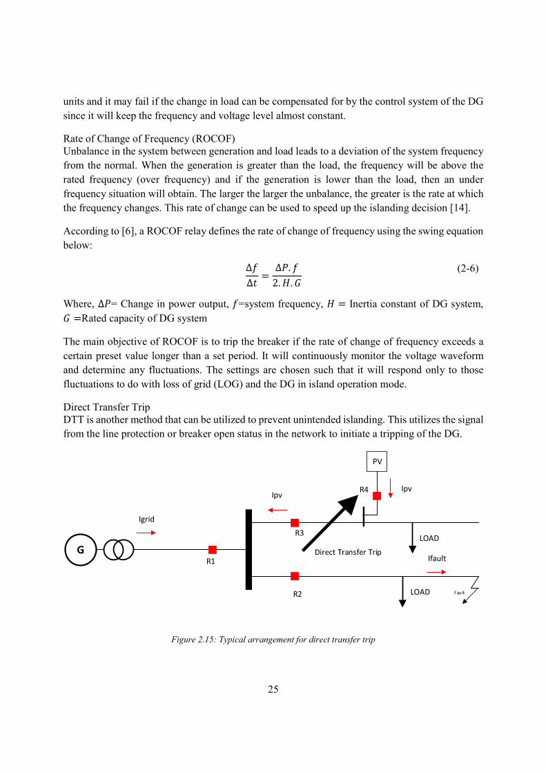
5.1.1 Direct Transfer Trip using wireless link................................................................... 59 5.1.2 Under voltage protection .......................................................................................... 60 5.1.3 Interfacing circuit ..................................................................................................... 60 5.1.4 Firing pulse circuit with protection disabling signal ................................................ 61 5.1.5 Rate of Change of Frequency Protection (ROCOF) ................................................ 63

5.2 Performance of the proposed solutions ........................................................................... 63 5.2.1 Direct Transfer Trip (Overcurrent protection with communication) ....................... 64 5.2.2 Under voltage Protection .......................................................................................... 65 5.2.3 ROCOF Protection ................................................................................................... 67 5.2.4 Summary of Scenarios, Effects and Proposed Solutions ......................................... 69

Chapter 6: Conclusion ans Future Work ........................................................................................ 71 6.1 Conclusions ..................................................................................................................... 71 6.2 Future Work ..................................................................................................................... 72

References ...................................................................................................................................... 73 Appendix A .................................................................................................................................... 77 Appendix B .................................................................................................................................... 78 Appendix C .................................................................................................................................... 81

xii

List of Figures

Figure 2.1: Overcurrent protection scheme ...................................................................................... 8 Figure 2.2: Trip and block regions for the overcurrent relay ........................................................... 9 Figure 2.3: Relay coordination for instantaneous overcurrent ......................................................... 9 Figure 2.4: Radial distribution system ........................................................................................... 11 Figure 2.5: Classification of PV systems ....................................................................................... 16 Figure 2.6: Diagram of grid-connected PV system ........................................................................ 16 Figure 2.7: Schematic diagram of a PV stand-alone system .......................................................... 17 Figure 2.8: Schematic diagram of a hybrid system ........................................................................ 18 Figure 2.9: Circuit to illustrate increases/reduced fault current ..................................................... 19 Figure 2.10: Distribution feeder with PV generator ....................................................................... 19 Figure 2.11: Distribution system with PV on feeder other than where fault is .............................. 20 Figure 2.12: Fault current contributions from the grid and a PV unit connected to a feeder ......... 20 Figure 2.13: Overcurrent relay: forward (F) and reverse (R) fault ................................................ 22 Figure 2-2.14: Techniques to detect unintentional islanding. ........................................................ 24 Figure 2-2.15: Typical arrangement for direct transfer trip ........................................................... 25 Figure 2-2.16: Distribution System with solar PV and fault location downstream ....................... 27 Figure 2-2.17: Thevenin equivalent circuit for Figure 2-17 without PV (left) and with PV (right) ........................................................................................................................................................ 27 Figure 3.1: CIGRE LV distribution network ................................................................................. 32 Figure 3.2: Pie section drop down menu ........................................................................................ 33 Figure 3.3: Inverter topology ......................................................................................................... 33 Figure 3.4: Sine reference generation circuit in PSCAD ............................................................... 34 Figure 3.5: Firing pulse generator .................................................................................................. 34 Figure 3.6: LC Line filter in PCAD ............................................................................................... 35 Figure 3.7: PV solar panel component in PSCAD ......................................................................... 35 Figure 3.8: PV array characteristics drop down menu ................................................................... 36 Figure 3.9: Relay Characteristic Figure 3.10: Relay Menu ....................................................... 38 Figure 3.11: Overcurrent protection arrangement .......................................................................... 38 Figure 3.12: CIGRE Network Model in PSCAD ........................................................................... 39 Figure 3.13: Typical MV network .................................................................................................. 40 Figure 3.14: Typical MV network as modelled in PSCAD ........................................................... 41 Figure 4.1: Methodology of study .................................................................................................. 43 Figure 4.2: CIGRE Network Upstream Faults ............................................................................... 44 Figure 4.3: CIGRE Network Downstream Faults .......................................................................... 44 Figure 4.4: MV Network Upstream Simulations ........................................................................... 47 Figure 4.5: MV Network Downstream Simulations ...................................................................... 48 Figure 4.6: Plot of trip time with and without solar PV up to hosting capacity ............................. 51

xiii

Figure 4.7: Variation of grid and fault currents with faults downstream, PCC at A, PV at 30% penetration ...................................................................................................................................... 53 Figure 4.8: Variation of grid and fault currents with faults downstream, PCC at E and PV at 30% penetration ...................................................................................................................................... 53 Figure 4.9: Variation of grid and fault currents with downstream fault, PCC at X and PV at 30% penetration ...................................................................................................................................... 54 Figure 4.10: Coordinated for fault currents at relay R3 vs. fault currents with PV upstream........ 54 Figure 4.11: Summary of results .................................................................................................... 57 Figure 5.1: Overcurrent protection with communication from upstream element ......................... 60 Figure 5.2: Under voltage protection circuit .................................................................................. 60 Figure 5.3: Protection interfacing circuit ....................................................................................... 61 Figure 5.4: Firing pulse circuit to include protection signal .......................................................... 62 Figure 5.5: ROCOF signal pickup .................................................................................................. 63 Figure 5.6: ROCOF protection ....................................................................................................... 63 Figure 5.7: Overcurrent protection and Direct Transfer Trip signals ............................................ 64 Figure 5.8: Upstream faulty feeder and PV current fault currents ................................................. 64 Figure 5.9: Grid and PV fault currents during fault ....................................................................... 65 Figure 5.10: Under voltage Response to high fault current contribution ....................................... 66 Figure 5.11: Inverter Instantaneous voltages after under voltage protection operation. ................ 66 Figure 5.12: Frequency excursions (above) and rate of change of frequency (below) during and after the fault .................................................................................................................................. 68 Figure 5.13: ROCOF and Upstream breaker signals ...................................................................... 68 Figure 5.14: Upstream and PV currents show instants of fault initiation and tripping .................. 69

xiv

List of Tables Table 2.1: Summary of impacts and solutions ............................................................................... 26 Table 2.2: List of available battery types and their advantages and disadvantages ....................... 29 Table 3.1: PV array parameters ...................................................................................................... 36 Table 4.1: Base Case Simulation Results for CIGRE Network ..................................................... 45 Table 4.2: CIGRE Network Upstream Fault Results ..................................................................... 46 Table 4.3: Upstream fault simulations, fault location at bus AC ................................................... 50 Table 4.4: Downstream, high fault current contributions, fault location at bus X ......................... 51 Table 4.5: MV fault analysis A ...................................................................................................... 55 Table 4.6: MV fault analysis, bus X ............................................................................................... 56 Table 5.1: NAND gate truth table .................................................................................................. 61 Table 5.2: Truth table for AND gate .............................................................................................. 62 Table 5.3: Summary of Scenarios, effects and proposed solutions ................................................ 69 Table A.1: Data for the CIGRE LV network ................................................................................. 77 Table A.2: Loads of European LV distribution network benchmark ............................................. 77 Table B.1: Line parameters of a typical medium voltage network ................................................ 78 Table C.1: Typical MV network fault analysis at B ...................................................................... 81 Table C.2: Typical MV fault analysis C ........................................................................................ 82 Table C.3: Typical MV fault analysis D ........................................................................................ 83 Table C.4: Typical MV fault analysis E ......................................................................................... 84 Table C.5: Typical MV analysis F ................................................................................................. 85 Table C.6: Typical fault analysis H ................................................................................................ 86

xv

xvi

List of Abbreviations AC Alternating Current BESS Battery Energy Storage BOS Balance of Systems CT Current Transformer CTI Coordination Time Interval DC Direct Current DER Distributed Energy Resources DG Distributed Generation DR Distributed Resource EMTD Electromagnetic Transients including DC EPS Electric Power System EOL End of Line IEEE Institute of Electrical and Electronics Engineers LV Low Voltage MPP Maximum Power Point MV Medium Voltage NP Network Protector PCC Point of Common Coupling PN Positive Negative PSCAD Power Systems Computer Aided Design PV Photovoltaic PWM Pulse Width Modulation ROCOF Rate of Change of Frequency SCC Short Circuit Capacity NVD Neutral Voltage Displacement

xvii

1

1 Introduction 1.1 Background Solar power has been developing from small applications to becoming a mainstream source of electric power [1]. The solar power industry has been growing globally. Dropping costs, as well as concerns like global warming and air pollution, have triggered massive growth in the solar energy industry. Major world economies, like USA, China, Germany, the UK, Spain, and many other countries are in the forefront in the growth of solar technology [2]. It is projected that the installed capacity of solar PV will double or even triple by 500 GW between now and 2020, and by 2050, solar power is expected to become the world’s largest source of electricity [3]. The reasons for this increased penetration of solar photovoltaic (PV) are: (i) the need to reduce carbon emissions on the energy systems, (ii) improve energy security, and (iii) increasing access to electricity to new consumers, especially in the third world [4]. Governments have moved into action at the international and national levels to create policies that promote renewable energies development. This is an effort to help reduce emissions [4].The main challenge is to ensure that the environment is preserved, climate change is arrested while at the same time energy is made readily available. Solar PV is a technology that has attracted a lot of research and its use in large power systems is increasing. The driving factors for this have been highlighted in the preceding paragraph. In addition, solar offers environmental benefits, low operating costs, and reduced dependence on fossil fuels. However, solar generation varies with solar insolation. This variability affects how distribution systems with high penetrations of renewable energy sources operate. This variability can be solved by using battery energy systems (BESS). The levels of solar PV and BESS penetration are expected to increase. The traditional power system is designed to have a passive distribution system with power flow in one direction only, from the transmission grid into the distribution grid and finally to the customer, without any generation at the customer end. The introduction of generation at the distribution/customer end interferes with power flows as a meshed network is now created. The challenges introduced into the system are in three groups, technical, commercial and regulatory [5]. The technical challenges are due to the high dependence of PV generation output on uncertain weather conditions which fluctuate fast. These include, among others, reversed power flow, voltage rise, grid stability, local network congestion, and relay protection. With regard to the protection system, the integration of PV can cause redistribution of the fault currents on the feeder circuits.

2

Such redistribution could result in higher current magnitude on the feeder during faults which in certain cases can exceed the rating fuses, breakers, etc. Changes in fault current and direction may also lead to a loss of protection coordination between multiple devices, desensitization of protection, undesirable/mal-tripping of relays, unwanted islanding, prevention of automatic reclosing, [6] etc. 1.2 Objectives The objective of this thesis is to investigate the impacts of solar PV on the protection system (e.g., on relay operation, settings, coordination) of low and medium voltage distribution networks and to propose solutions to the problems. This will be done by modelling the CIGRE low voltage and a typical medium voltage distribution network in Sweden. Two cases will be studied, with and without solar PV power. The simulation software used in this thesis is Power Systems Computer Aided Design with Electromagnetic Transients including DC (PSCAD/EMTDC). The thesis investigates how the overcurrent protection coordination and how fault current levels are affected when solar PV is present in a distribution system. Further, the theoretical hosting capacity as regards protection is also determined. Lastly, solutions are proposed to mitigate the impacts that are identified. 1.3 Scope The thesis covers the impacts that solar PV has on the overcurrent protection coordination of a distribution network. Two distribution networks are modelled in PSCAD. Simulations and studies have been carried out without solar PV to determine the performance of the overcurrent protection system. After that, the solar PV model was added to the models and the performance of the overcurrent protection ascertained again. The thesis investigates the impacts of PV on the protection system performance using PSCAD simulation software. The studies are limited to the low voltage system of 400V and medium voltage network of 20 kV. The following factors are worth noting concerning this thesis:

The variation of solar PV with solar insolation is not considered, only the steady state contribution of solar PV is considered. Therefore, the solar PV unit developed has a constant irradiance and a constant temperature. Consequently, the maximum power point tracking is not implemented in the solar PV model developed here.

The transient nature of faults is not considered, only the steady state effects of faults are studied.

The two networks involved are radial systems and not meshed networks without any other types of Distributed Energy Resources (DERs) other than the integrated solar PV.

3

The overcurrent models developed do not use current transformers (CTs) to provide a signal to the relay, rather, PSCAD/EMTDC has a measured signal which can be used, this takes the function the CT is supposed to perform.

The networks are connected to an electricity grid. 1.4 Report Structure This thesis report is divided into six chapters.

Chapter 2 reviews the literature around the subjects covered in the thesis, namely; system protection, overview of PV systems, PV systems and applications, requirements to connect PV system to a utility grid, battery energy storage systems, and impacts of connecting solar PV to the distribution grid.

Chapter 3 looks at the development of the model in PSCAD and also describes the simulations carried out. The study methodology is highlighted in this chapter.

Chapter 4 presents the impacts of PV on distribution system protection. Chapter 5 discusses the proposed solutions to address the impacts and also the performance

of these solutions. Chapter 6 contains the conclusions that have been made from the study and also possible

topics for future study are suggested.

4

5

2 Protection system, Solar PV and its impacts on protection system and possible solutions In this chapter, the literature that has been used to discuss the main concepts in the study is presented. The concepts of the need and requirements of protection, protection schemes for a distribution network, solar PV schemes and some of the impacts that solar PV integration causes to the grid in general, and to overcurrent protection coordination in particular are discussed. Protection with distributed generation at the distribution level is also discussed, including current practices for distribution system protection. The chapter further highlights the solutions that are currently under research or implementation to address these challenges. 2.1 Protection System A power system is designed to generate, transmit and distribute electric power to the end customer in a secure and reliable manner [7]. Generation, involving conversion from one form of energy e.g. nuclear, hydraulic, to electrical energy, is usually at a lower voltage level which is then transformed, using transformers, to a higher voltage level for transmission. The transportation of this energy is done through the transmission system to geographically faraway places called load centres, where loads are situated. After the voltage is stepped down to a suitable level, it is then distributed to customers for consumption. The equipment which is used in the generation, transmission, and distribution of power is costly equipment of a complex nature. In order to ensure that this equipment and the lives of people are safeguarded, as well as to ensure provision of reliable service, there is need to provide protection to be able to detect various fault conditions and address them, such as isolating a faulty section while the rest of the system continues in operation. A protection system, according to NERC, is defined as “protective relays, associated communication systems, voltage and current sensing devices, station batteries and dc control circuitry [8]”. At the heart of the protection system is the protective relay which is a device that detects faults and relays a signal to a disconnect device to operate and isolate faulty section. According to the IEEE’s definition, a relay is “an electric device that is designed to interpret input conditions in a prescribed manner, and; after specified conditions are met, to respond to cause contact operation or similar abrupt changes in associated electric control circuits [9]”. The IEEE further defines a protective relay as “a relay whose function is to detect defective lines or apparatus or other power conditions of an abnormal or dangerous nature and to initiate appropriate control

6

circuit action [9]”. Relays acquire various types of signals from the power system. These signals can be electrical, magnetic, heat, pressure, etc. The relay will process them with a designed process or algorithm. Protection has certain requirements for it to be able to perform its functions properly. These are: sensitivity, selectivity, speed, reliability and cost. Various types of equipment are used to protect distribution networks. The particular protection scheme used depends on the voltage level, the element being protected and the network configuration. Distribution networks are mainly protected by overcurrent protection because of their radial nature. This is protection that operates when current in the system exceeds a predetermined value. These currents, several times higher than the maximum load current, are usually caused by faults and the system must be protected against the damage caused by them. When the load current exceeds a pre-set value, a signal is sent to operate protective devices. Protective devices on the system include thermomagnetic switches, moulded-case circuit breakers (MCCBs), fuses and overcurrent relays [10]. Distribution system protection consists of fuses, relays, sectionalizers and reclosers [11]. 2.1.1 Fuses A fuse is an overcurrent protective device that opens up a circuit in which it is connected and breaks the current when a certain value is exceeded. It has an element which is heated by the passage of current, this element melts at a given predetermined value of current. A fuse operates by the destruction of the fuse element [10]. An element, which is a conductor of given cross-section is heated by current passing through it until it melts. The time it takes for this action is represented in a time/ current characteristic curve. On melting, a break is caused in the element, at which an electric arc is established, which burns in the fuse until the current returns to zero. A fuse operates in two stages: (1) the pre-arcing time (2) the arcing time. Pre-arcing time This is the time period from the start of the current that is large enough to melt the fusible element in a fuse and the time that an arc emerges. Consider a conductor having resistance , the current passing through it is A for a time . This conductor will be heated by the passage of this current, the quantity of the heat being released in the conductor is . Joules are liberated for every ohm of conductor. For a varying current over a period, ʃ Joules will be released. This is integral is abbreviated as . It is used to estimate the heating effect on a protected circuit due to a very short pulse of heavy current [10].

7

The heat generated due to the passing of the prospective current is all used to heat the element to its melting point at its narrowest constriction. The required to melt the element is constant and independent of current. This is called the pre-arcing [10]. It is related to the amount of energy that is let through by the fuse element upon clearing a fault. Fuse manufacturers provide the data in charts and it is used to perform coordination with upstream or downstream devices. Both melting and clearing are specified in the data. The

is proportional to the amount of energy required to begin melting the fuse element. Arcing time This is the time period between the time the arc is generated, until the time it is finally extinguished. Types of fuses Different types of fuses exist. These are:

1. Dual-Element, Time-Delay fuse 2. Dual-Element, Time-Delay fuse, Current-Limiting fuse 3. Fast-Acting, Current-Limiting fuse (Non time-Delay)

Dual-Element, Time-Delay Fuse This fuse provides time delay in the low overload range to eliminate unnecessary opening of the circuit. It is made up of one or more fusible elements (links) connected in parallel: an overload (s) and short circuit elements. The fusible elements are then connected in series with an overload trigger assembly. The overload element opens when the current exceeds 110 percent of the fuse’s rating for sustained period of time. The fuse can handle up to five times its current rating for a period of 10 seconds. The short circuit element opens in the event of a short circuit or ground fault. These kinds of fuses can be used for mains, feeders, sub feeders, branch circuits, motor circuits and circuits having a high inrush characteristics. Dual-Element, Time-Delay, Current-Limiting fuse These operate in the same way as the dual-element time delay fuses and can be used for the same applications. Under the dual-element, time-delay, current-limiting fuse, the fuse opens extremely fast under short circuit faults. Fast-Acting, Current-Limiting fuse This type of fuse has an extremely fast response in both low-overload and short circuit ranges and reduces the high-fault current magnitude to a value less than what it would be had there been no fuse or breaker in the circuit. It is used to provide better protection in terms of adequate interrupting rating to mains, feeders, sub feeders and other components.

8

2.1.2 Overcurrent Relays Three types of overcurrent relays exist according to their operating characteristics [10]:

i. Instantaneous overcurrent: The relay operates instantaneously to send trip signal to breaker when the current exceeds a predetermined value.

ii. Time discrimination: An appropriate time setting is given to each of the relays controlling circuit breakers in the circuit such that the relay closest to the fault operates first.

iii. Time delay overcurrent (TOC): Operates on the basis of a current vs. time curve. If the current level exceeds a pre-set value for a certain amount of time, then the circuit breakers get the command signal to trip.

Overcurrent relays are usually supplied with an instantaneous element and a time-delay element within the same unit [1]. When setting overcurrent relays, three phase short-circuit currents are used for setting phase relays and phase-to-earth fault current used for setting earth-fault relays. Relay design can be categorised based on principle of operation. These are categorised as [12]

i. Electromechanical: which uses the induction disk principle, electromagnetic action of a solenoid

ii. Static: opening and closing of relay contacts is done by semiconductor switches e.g. thyristors

iii. Mechanical: relay operation by mechanical displacement of different gear level system The overcurrent relay trip coil is fed by current on the secondary side of the current transformer I’ as shown in Figure 2.1.

Figure 2.1: Overcurrent protection scheme

Breaker contacts

Relay operating coil

Manual trip

Breaker trip Battery

I’

Relay contacts

I

9

Instantaneous over current relays operate on the current magnitude. If the CT secondary current exceeds a certain level (pick up current), the relay contacts close which energizes the circuit breaker trip coil and leads to the opening of the circuit breaker. Otherwise the relay contacts remain open which leaves the trip coil open. This is illustrated in Figure 2.2 below. The difference in impedance between the source and the fault determines the fault current variation. Relay nearest to the fault is set to trip its breaker first.

Figure 2.2: Trip and block regions for the overcurrent relay Two important aspects that affect this method of coordination are:

i. It may be hard to distinguish between a fault at points F1 and F2, as shown in Figure 2.3, since the distance between them is small corresponding to a current change of approximately 10%.

ii. There are variations in the fault current at the source. At lower fault levels, the current might be too small to be detected by the relays.

Figure 2.3: Relay coordination for instantaneous overcurrent

Im I’

Re I’ Block

Trip

F1 A B C F3 F4 F2

10

Time delay overcurrent operates on the magnitude of the CT secondary current but with an intentional time delay. The delay is dependent on the ratio of the CT secondary current to the pickup current. The higher the ratio, the lower the delay time and vice versa. Operating time is set based on curves of operating time vs. current (usually given as a ratio of measured current to pick up current). If current is less than the pickup current, then the relay remains in the block position. Choice of relay time-current characteristics depends on the sources, lines and loads. 2.1.3 Reclosers A recloser is a protective device on the distribution system which has the ability to detect overcurrent situations in phase and phase-to-earth fault conditions. It ensures that the distribution system is not unnecessarily disconnected for temporal faults. When an overcurrent occurs and persists for a certain time, the recloser can interrupt the circuit and automatically reclose to re-energise the line. It will stay open if the original fault persists to isolate the fault [10]. They are typically designed to have up to three open-close operations before lock out. Coordination of the recloser with other protection devices is done to ensure that only the smallest possible portion of the network that ensures isolation of the fault is disconnected. 2.1.4 Sectionalizers A sectionalizer has an inherent ability to isolate faulty sections that have been disconnected by the operation of an upstream circuit breaker or recloser. Sectionalizers have no current breaking capability and hence are usually installed on the downstream of a recloser or breaker. The sectionalizer counts the number of times the recloser has operated and when a predetermined number is reached, with the recloser in open position, it opens to isolate the faulty section. Sectionalizers do not have a time/current operating characteristic [10]. 2.2 Radial Network Overcurrent Protection Coordination. This is the process of determining the best timing for the interruption of current when abnormal or fault conditions occur. The objectives are to determine the characteristics, ratings, and settings for overcurrent protective devices in order to minimize equipment damage and interrupt short circuits as rapidly as possible [13]. The goal is to ensure that only a minimum portion of the system is disconnected in as afar as is necessary to eliminate the fault, ensuring that the maximum number of loads continue to be supplied. Coordination should be done in such a way that the device closest to the fault must trip first, that is, offers primary protection. The next device in line offers backup protection. If primary protection does not protect the system, then backup protection must trip the system. Considering Figure 2.4, the relays are coordinated in the upstream direction, whereby the units furthest from the grid connection are configured to operate first for the fault shown. A fault is cleared by opening of the breaker immediately to its left side. In this case, CB4 should trip first, if not, CB3, CB2, or CB1 in that order for a fault on the downstream.

11

AC

CB1 CB2 CB3 CB4

Figure 2.4: Radial distribution system

The power system is divided into zones of protection. The boundary of the zone is defined by current transformers. Relays and breakers form pairs and are responsible for clearing faults in their protected zone and also act as backup for the zone downstream. Relays are coordinated in such a way that when a fault occurs, the breaker most remote from the source operates in the shortest time. Circuit breakers towards the source being tripped in progressively longer times. This difference in operating time between two adjacent breakers is known as grading margin or coordinating time interval, CTI. CTI allows time for the fault to be isolated before backup units are tripped. Overcurrent protection relays can be definite-time or inverse-time. Inverse-time protection offers shorter tripping times. The relay furthest downstream is not coordinated with any relay and hence is typically a definite-time unit. Zones of protection possess the following features:

zones overlap overlap regions denote circuit breakers all circuit breakers in a given zone will operate when a given fault occurs

Overlapped regions are made up of two sets of instrument transformers and relays for each circuit breaker. These are designed to eliminate unprotected zones in the system however they are designed to be as minimal as possible such that in case of a fault the isolated areas containing (both areas containing circuit breakers). 2.3 Protection with distributed generators at the distribution level There are some major differences in fault current contributions with DER and conventional energy sources. Three main causes of these differences, according to [14], are:

i. Conventional energy sources are centrally located while DER are distributed around the electric network. In the event of a fault, for systems with DER, there are short circuit current contributions from directions not originally considered for the conventional protection schemes. Also, unexpected load flows can cause ‘blinding’ or ’sympathetic tripping’. Blinding is the phenomenon where, with DER fault current contribution in the system, fault current from the central connection point to the transmission network is reduced which may

12

result in delayed or unselective tripping of protection. Sympathetic tripping is where DER fault current contribution causes tripping of a relay in its connection path.

ii. Many DER are coupled to the network via inverters whose SCC is limited to values not much higher than the nominal ratings of the inverter. Therefore, SCC of grids dominated by inverter-coupled generators to the grid are significantly lower than of grids with rotating generators (synchronous or induction machine) of the same rating.

iii. The lower SCC is connected to a different time characteristic of the SCC. Another difference between conventional and DER connected networks is behavior of fault transients. Different transients generated by inverter controllers could affect operation of some relays e.g. the direction determination [14]. 2.4 Current practices in distribution system protection Current practices of distribution system protection vary among countries. Whereas the protection scheme can be the same, certain practices in different countries create the disparity. Some of the practices include [14]:

Functions within the protection scheme: Some countries can allow a certain level of fault current on the systems while others prefer to eliminate any fault on the network.

The network structure National regulatory legislation Protection functions’ configurations

The protection function can be divided into two basic categories [14]: i. Short circuit protection: prevents thermal and mechanical asset stress and damage caused

by short circuit current ii. System protection: protects power grid from unacceptable operating conditions

Overcurrent protection is usually sufficient to protect feeders in radial networks, in some countries e.g. Austria, Germany, Spain and Denmark, distance protection is used for meshed networks. Reverse interlocking can be used as an added feature. This is where feeder protection operates much faster to isolate faults on busbars, as long as the respective feeder they are protecting is in a healthy condition. Another scheme applied on the distribution network is the overcurrent earth fault protection. Phase to ground faults cause earth fault current to flow. The magnitude of this current is much lower than the phase fault current due to the higher fault impedance of the earth faults than for the phase faults [15]. This calls for a separate relay on the neutral line to keep current through the line at safe levels. In France, zero sequence watt metric protection function is used for earth fault protection [14].

13

For system protection, different levels of the over- and under frequency protection and voltage protection are used in all countries. These protection schemes disconnect DER from the network once a deviation from the normal operating conditions of the network are detected. In some countries e.g. France, an islanded section of the network prompts a signal that trips the circuit breaker of the large DER for disconnection from the grid. In other countries, islanded network operation doesn’t cause disconnection of DER provided the frequency and voltage remain within acceptable levels. 2.5 Methods for distribution system protection with distributed generators In addition to already existing protection schemes, new approaches need to be adopted to protect distribution systems with integrated energy sources. Some of the approaches are described below [14].

Islanding detection (tele-decoupling): detection of the opening of the MV feeder protection and communication to the DER decoupling protection to disconnect DER

DER facility protection: this is protection against faults within the DER installation DER facility decoupling protection: protection to disconnect DER facility from the rest of

the network when a fault on the MV feeder occurs. Directional phase protection: overcurrent protection with a directional feature that responds

to overcurrent for a particular direction flow. HV neutral displacement voltage protection: this is another decoupling protection used

when there is back feed or islanding and continued supply of an isolated HV network via delta winding distribution transformer. Since there is no earth fault path through the transformer, Neutral Voltage Displacement (NVD) protection will be required on the high voltage side of the transformer.

2.6 Overview of PV Systems The PV system is composed of many components that work together with the aim of producing electric energy. This energy could be supplied to the electricity grid, supply a household, power a handheld calculator, etc. The design of the system is determined by the intended task, the location and conditions at the site at which it will be used [16]. This section discusses the components of the PV system. The main components are PV array (which includes the modules, wiring and mounting structure), storage equipment (if required), power conditioning and control equipment and load equipment. The array is made up of the photovoltaic part (PV modules) and the balance of system (BOS) components [16]. 2.6.1 The PV Cell The basic building block of a photovoltaic (PV) cell is a p-n junction. It is a semi-conductor device that coverts solar energy into direct-current electricity. A property called photoelectric effect is

14

possessed by certain materials, giving them the ability to absorb photons of light and emit electrons [17]. The junction consists of differently doped semiconductor elements from group V of the periodic table, such as silicon or germanium, on each side. Usually on the n-side, silicon gets moderately doped by phosphorus or other elements of the group V of periodic table resulting in a material with electrons as excessive carriers. For the p-side silicon is doped by gallium or indium or other elements of the group III of the periodic table, resulting in a mixture with lack of electrons, or equally with excessive positive carriers called holes. When n-type and p-type materials come in contact, excess carriers from one side flow to the other side until a characteristic equilibrium is reached. This way an electric field is built up along the contact area called the depletion region [18]. When the above p-n junction is exposed to light, it produces electrons that are proportional to the oncoming light. The larger the surface area, the larger the exposure and therefore, the larger the current produced. The p-n junction is constructed as thin plates or cells that have a large surface area. Each of such cells are made up of wafers of n-type and p-type silicon that are in contact with one another. On both sides of the wafers, there are electrical connections that are responsible for conducting the electrons. A non-reflecting layer is above the n-type wafer to ensure that as much light as possible is gathered in the silicon material. The top layer is toughened glass that protects against the elements of the weather while the bottom layer is a strong plate to mount the entire structure. 2.6.2 The PV Module When solar cells are electrically connected together, they form a module. The connections can be in series or in parallel to produce a specified voltage or current respectively [19] , [20]. This is done to increase their power output. The typical number of series connected cells is usually 36, which are encapsulated into a single unit. The encapsulation is to provide protection for the cells from the harsh environment in which they operate [18], [20]. Modules have capacities of between 50W to 200W. Each module is enclosed in an aluminum frame. 2.6.3 The PV Array When several modules are electrically connected together and mounted in the same plane, they form a solar panel [21], [20]. The array also includes the support structure, in addition to the modules. These arrays can be of sizes ranging from a few hundred watts to hundreds of kilowatts. These modules can be connected in series to increase the voltage, or in parallel to increase the current, depending upon the load requirement. When PV modules are combined with additional application-dependent system components (e.g. inverters, sun trackers, batteries, electrical components and mounting systems), they form a PV system, which is highly modular, with capacities ranging from a few watts to tens of megawatts [22] [20]. 2.6.4 The Inverter The inverter is defined by the IEEE as “Equipment that converts direct current (dc) to alternating current (ac). Any static power converter (SPC) with control, protection, and filtering functions used

15

to interface an electric energy source with an electric utility system” [23]. The inverter is a key component which forms the interface between the PV generator and the electricity grid [24] or the AC loads. The performance of the inverter has vital significance for grid-connected PV power plants. It has direct influence on whether the PV power plant can meet the requirements for grid operation. Inverters are supposed to have low voltage ride through (LVRT) and flexible active and reactive power control capabilities [22]. The LVRT is a requirement that a unit connected to the grid should meet, in case of a fault or a voltage dip. Inverters are classified into stand-alone and grid-connected inverters [16]. The stand-alone inverter is independent from the grid in its operation. It has an internal frequency generator to obtain the correct output frequency, whereas for the grid-connected inverter, it has to be able to integrate properly with the grid in both voltage and frequency [16]. The inverter is an electronic component and works as a system and energy manager carrying out the following functions [24]:

Converts the DC generated by the PV generator into AC required by the grid Maximum Power Point (MPP) tracking. The MPP tracker supplies the grid with the

maximum output all the times. The inverter voltage is compared with the current generator MPP voltage continuously

Provides protection to the PV generator and the electricity grid Acts as an interface for communication and operations monitoring

2.6.5 Power Conditioning The system needs to operate at its optimum. In order to achieve that, it is essential that power conditioning equipment is included in it. The PV array will deliver its maximum power output if it operates at the maximum power point. In solar PV generation, the generation varies with the insolation of the sun and temperature, therefore, at maximum power point, the current and voltage vary. In order for the array to operate at the maximum power point, there is need to track this maximum point. The control equipment to achieve this objective is called the Maximum Power Point Tracker (MPPT). The MPPT controls the effective load resistance that the PV array sees. This controls the system operating point on the I-V characteristic. In a grid-connected system, the MPPT is included in the inverter [16]. 2.7 PV Systems and Applications Solar PV systems are generally classified according to how they function and what the operational requirements are, how the components are configured, and how the equipment is connected to the other power sources and electrical loads (appliances) [25]. Figure 2.5 shows the different kind of PV systems available. The broad classifications are Grid-connected and Stand-alone Systems. If the PV system is used in conjunction with another power source like a wind or diesel generator then it falls under the class of hybrid systems.

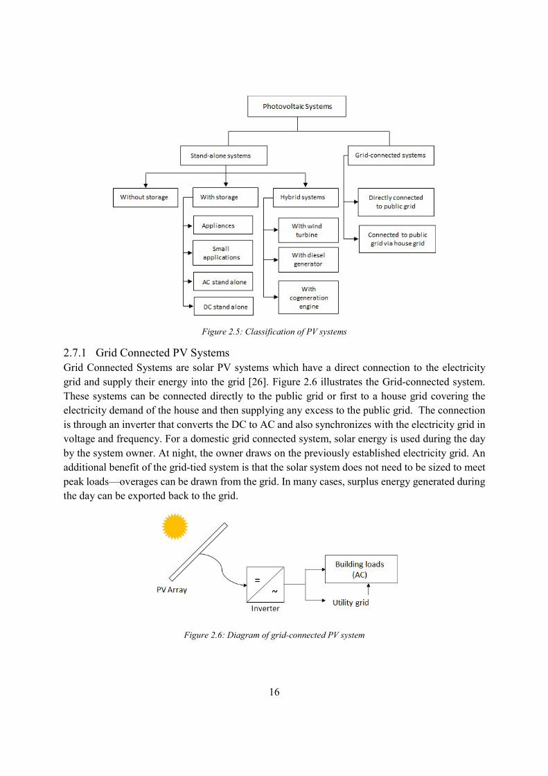
16

Figure 2.5: Classification of PV systems

2.7.1 Grid Connected PV Systems Grid Connected Systems are solar PV systems which have a direct connection to the electricity grid and supply their energy into the grid [26]. Figure 2.6 illustrates the Grid-connected system. These systems can be connected directly to the public grid or first to a house grid covering the electricity demand of the house and then supplying any excess to the public grid. The connection is through an inverter that converts the DC to AC and also synchronizes with the electricity grid in voltage and frequency. For a domestic grid connected system, solar energy is used during the day by the system owner. At night, the owner draws on the previously established electricity grid. An additional benefit of the grid-tied system is that the solar system does not need to be sized to meet peak loads—overages can be drawn from the grid. In many cases, surplus energy generated during the day can be exported back to the grid.

Figure 2.6: Diagram of grid-connected PV system

17

2.7.2 Standalone Systems Stand-alone systems are solar PV systems which are independent of any electricity grid. The energy yield must be sized to meet the load requirements. They are usually fitted with energy storage systems to absorb surplus energy and to meet the demand when the solar irradiation is not enough. Stand-alone systems are usually implemented in rural and remote areas in developing countries where no access to the electricity grid is available or costly to implement. They are also used in various applications in industrialized countries as well (e.g. roof top systems, PV-glazing, solar traffic lighting, traffic infrastructure, solar chargers, mobile communication transmitters et al.). The grid-connected systems, which are PV systems connected to the local distribution grid and supply it with power. Figure 2.7 shows a stand-alone system.

Figure 2.7: Schematic diagram of a PV stand-alone system

2.7.3 Hybrid Systems To meet the largest power requirements in an off-grid location, the PV system can be configured with a small diesel generator. This means that the PV system no longer has to be sized to cope with the worst sunlight conditions available during the year. Use of the diesel generator for back-up power is minimized during the sunniest part of the year to reduce fuel and maintenance costs.

18

Figure 2.8: Schematic diagram of a hybrid system

2.8 Impacts of solar PV to the Distribution System Protection The traditional distribution system is passive and radial in nature, which is usually characterized by a single source on the upstream end, supplying a network of feeders on the downstream end. Protection for this conventional distribution system assumes a radial system such that the grading of the protection starts from the downstream end through to the upstream end. F. Katiraei et al [27] say that the impacts of DG can be local (e.g., feeder or substation) or system wide, depending upon the degree of DG penetration levels. The nature of these impacts can be steady-state or dynamic. With the connection of solar PV (and other DG sources) in the network, according to both [27] and [28] the system may lose its passive, radial nature and therefore, protection coordination may not hold. References [5], [26], [25], [29], [30] [31] and [32] highlight impacts due to the presence of DG in a distribution system. The preceding sections explain these impacts. 2.8.1 Increased Fault Current Figure 2.9 shows a distribution feeder with DG on the upstream of the R3 and a downstream fault. The fault current through R3 is a sum of the grid current and the PV unit current. The fault current is greater than that which passes through R3 in the absence of DG. This condition is not protected against in a traditional distribution system. The fault current has increased as seen by R3. In this case, coordination between R3 and upstream relays may be lost. 2.8.2 Reduced fault Current When a generator is added along a feeder, the fault current at the beginning of the feeder is reduced for a downstream fault. Considering the relay R1 at the start of the feeder in Figure 2.9.The relay will fail to operate when the fault current falls below the relay settings in the case were the PV unit is contributing a high enough fault current. This situation is aggravated for long feeders where the

19

fault current for a remote fault is low already. For definite-time overcurrent, protection will not operate for certain faults, while inverse-time relays will take long to clear the fault [31].

PV

Ifault

IpvIgrid

R2

R1G

R3

Figure 2.9: Circuit to illustrate increases/reduced fault current 2.8.3 Blinding of protection Considering Figure 2.10, R1 may not detect a downstream fault if the fault current contribution from the PV is high. The level of current through R1 may reduce to a level below the pickup value

PV

Fault

Ifault

IpvIgrid

R2

R1G

Figure 2.10: Distribution feeder with PV generator

2.8.4 Unwanted operation/Nuisance tripping For a fault on a feeder other than where the generator is connected, the breaker on the feeder where the generator is connected may result in unwanted operation due to fault current contribution by the PV generator [31]. Figure 2.11 shows a circuit where the fault is on a feeder other than the one on which a PV unit is connected. When a fault occurs, the DG will contribute to the fault current and a reversed fault current will be experienced through relay R3. The relay may trip the healthy feeder in a case of sympathetic tripping.

20

PV

LOAD

LOADIfault

Ipv

IgridIpv

R1

R3

R2

R4

G

Figure 2.11: Distribution system with PV on feeder other than where fault is

2.8.5 Non-controlled islanding One of the more serious consequences of introducing DGs to the network is the concept of unintentional or non-controlled islanding [14]. This is a situation where a portion of the network which has a DG is disconnected from the rest of the network. As highlighted in [31], non-controlled islanding can be initiated by a fault on the feeder and the upstream fuse or breaker opens and also by the opening of an upstream breaker or fuse without any fault present in the system.

PV

Fault

Ifault

IpvIgrid

R2

R1G

Figure 2.12: Fault current contributions from the grid and a PV unit connected to a feeder

A generator connected through a power electronics converter normally contributes too small a current to a fault for the overcurrent protection to detect it. In Figure 2.12 above, the fault current contribution by the grid, , is sufficient to be detected by R1 and trip the associated breaker while that by the PV, , is insufficient to be detected. The PV unit will continue feeding the fault. The fault may either clear by itself if the current becomes too small or the fault current may be maintained. When the fault current is maintained, the generator will go into non-controlled islanding. The balance between generation and the load in non-controlled islanding will determine the voltage and frequency magnitudes [31].

21

2.8.6 Unsynchronized Reclosing This explanation is a continuation of the explanation in section 2.8.5 after the PV unit has islanded. Automatic reclosing is often used with overhead feeders. From Figure 2.12 the CB at R1 will be reclosed after a certain time interval, with the DG still connected while the fault is cleared. This connects two systems that are out of synchronism, having different frequencies, voltages and phases. This leads to equipment damage due to the large currents that will be experienced [31]. 2.9 Proposed Solutions Research has been going on to find effective solutions to the aforementioned problems. Various literature propose several new approaches to solve the overcurrent coordination problem. This section highlights the various proposed solutions. 2.9.1 Increased Fault Currents To solve the problem of increased fault currents, the following approaches have been considered:

Tang et al. [33] proposes using a fault current limiter (FCL) to limit the impact that DGs have on relay protection coordination during a fault. A fault limiter limits the DG current during a fault and allows normal current flow when there is no fault [33]. Fault limiters are devices that have low impedance that produce no action during normal operation [34]. When a fault occurs, the FCL device acts quickly to insert a high impedance in series with the distribution network. This limits the fault current to a preset value [33].

Another approach is suggested by Khederzadeh [35]. It involves using a thyristor-controlled series capacitor (TCSC) as an FCL to restore the original relay settings. The TCSC in this case operates in the fault current limiting mode to limit the DGs fault current contribution without disconnecting the DG during a fault.

2.9.2 Reduced Fault Currents This can be mitigated for using FCL as described above. The FCL limits the fault current that the PV unit contributes to the fault. This causes the upstream relay to detect the right level of fault currents. 2.9.3 Blinding of protection This can be solved by FCL and under voltage protection. Additionally, the method of obtaining new relay coordination status can be used. This is an approach in which mathematics and computer-based methods are used to find new relay coordination methods for distribution networks with DG [34]. Zayandehroodi et al. [34] identify the following three methods in this category:

adaptive protection scheme for distribution networks with DG, multi-agent protection scheme for distribution networks with DGs and

22

expert system for protection coordination of distribution networks with DGs. Adaptive protection is a new concept. This is the ability of a protection system to respond to changing power system conditions by automatically altering its operating parameters to provide reliable relaying decisions [34]. Brahma and Girgis [36] came up with an adaptive protection scheme that involves dividing the network into zones. Each zone to have a balance of load and DG. The main relay is computer-based, with capabilities for high processing power, large memory and communication capabilities. The relay can sense a fault, determine the fault type and the associated zone. It would then isolate the affected zone. 2.9.4 Reverse Fault Current This problem is solved using directional overcurrent relays. An approach for protecting meshed distribution systems with DGs was proposed by [37] in which dual setting directional over-current relays (DOCRs) are used. They are equipped with two inverse time-current characteristics. Their settings will depend on the fault direction. They have different settings for forward and reverse directions. The protection coordination problem is formulated as a nonlinear programming problem whose objective is to minimize the overall operating time of the relays during both primary and back-up operation. 2.9.5 Current-only Directional Overcurrent Relay In reference [38], the authors indicate that the use of non-directional relays requires a number of relays and increases the complexity in the coordination settings. Using directional overcurrent relays reduces the number of non-directional relays and the complexity of relay settings is reduced. Traditional directional overcurrent relays however, have a voltage sensing element, that is, use voltage polarization [38] to detect the direction of the fault. They require both current and voltage measurement. For smart grids, more of these relays have to be used, making cost an important factor. The authors of [38] propose a novel current-only direction principle.

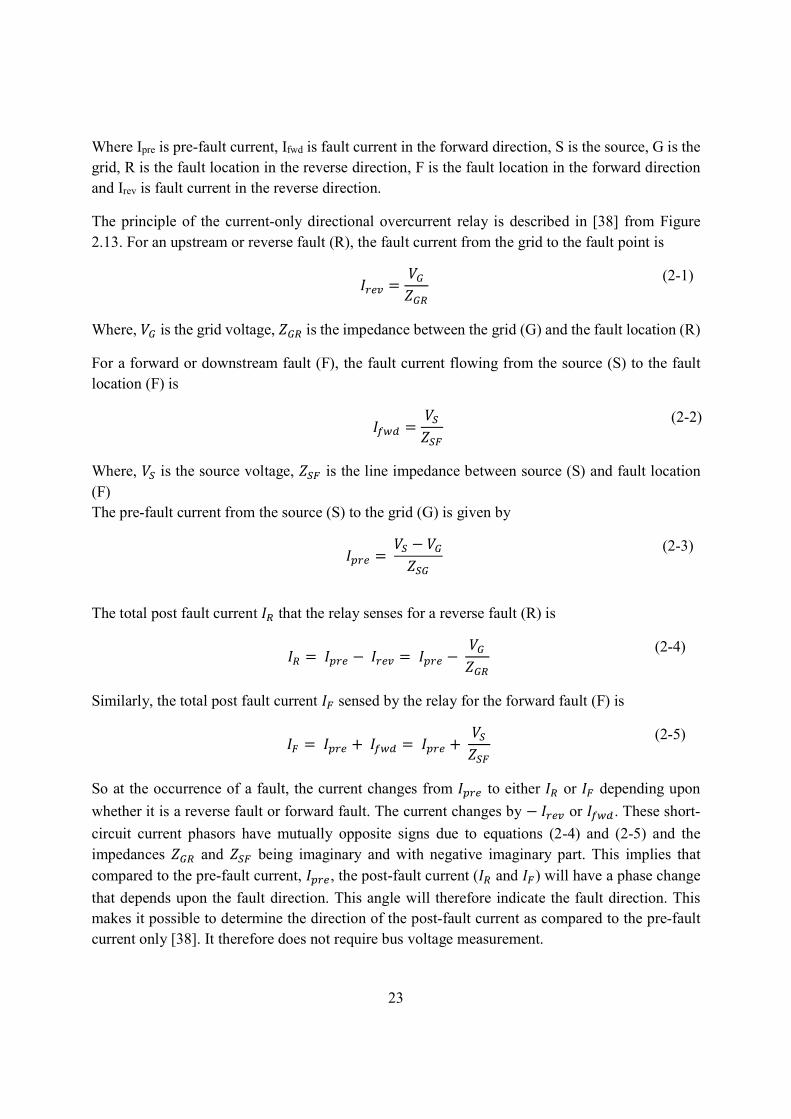
Figure 2.13: Overcurrent relay: forward (F) and reverse (R) fault

Irev

G S

Grid

G Source

Substation F R Ipre Ifwd

Relay

23

Where Ipre is pre-fault current, Ifwd is fault current in the forward direction, S is the source, G is the grid, R is the fault location in the reverse direction, F is the fault location in the forward direction and Irev is fault current in the reverse direction. The principle of the current-only directional overcurrent relay is described in [38] from Figure 2.13. For an upstream or reverse fault (R), the fault current from the grid to the fault point is = (2-1)

Where, is the grid voltage, is the impedance between the grid (G) and the fault location (R) For a forward or downstream fault (F), the fault current flowing from the source (S) to the fault location (F) is = (2-2)

Where, is the source voltage, is the line impedance between source (S) and fault location (F) The pre-fault current from the source (S) to the grid (G) is given by = − (2-3)

The total post fault current that the relay senses for a reverse fault (R) is = − = − (2-4)

Similarly, the total post fault current sensed by the relay for the forward fault (F) is = + = + (2-5)

So at the occurrence of a fault, the current changes from to either or depending upon whether it is a reverse fault or forward fault. The current changes by − or . These short-circuit current phasors have mutually opposite signs due to equations (2-4) and (2-5) and the impedances and being imaginary and with negative imaginary part. This implies that compared to the pre-fault current, , the post-fault current ( and ) will have a phase change that depends upon the fault direction. This angle will therefore indicate the fault direction. This makes it possible to determine the direction of the post-fault current as compared to the pre-fault current only [38]. It therefore does not require bus voltage measurement.

24

2.9.6 Islanding Detection Non-controlled islanding is supposed to be detected and the generating units disconnected in the islanded portion. This must be done in the shortest time possible. Reference [14] states that the DER must be disconnected for any of the following conditions:

The voltage and frequency being out of the contractual range; One or more phases of the transmission network is missing; Before the first reclosure in cases of automatic reclosure.

There are various ways in which this can be done, though there is no islanding detection technique that is recognized as truly efficient [14]. According to [14], three techniques identified as state of the art can be used to detect unintentional islanding, namely: Passive protection, Active protection and Network communication based protection. Figure 2.14 graphically shows the various types of protections that can be used to detect unintentional islanding.

Figure 2.14: Techniques to detect unintentional islanding.

In this thesis, we consider only under voltage, rate of change of frequency (ROCOF) and direct transfer trip (DTT) protections as the anti-islanding protections. Under/over voltage protection When the portion of the network with distributed generation is isolated, the generation sees it as a change of load and therefore network parameters change [14]. These network parameters are voltage and frequency. The level of unbalance determines the level of these parameters. When there is an unbalance between the load and generation, the under/over voltage protection may operate. Reference [6] states that this method provides an acceptable level of protection for small

Local

Under/over voltage/frequency protections Rate of Change of Frequency (ROCOF) Voltage Vector Shift Reverse reactive power flux

Active Detection

Passive local based

measurement

Comparison of rate of change of frequency protection (COROCOF) Direct Transfer Trip

Network Communication

Reactive power export error Fault level measurement System impedance

25

units and it may fail if the change in load can be compensated for by the control system of the DG since it will keep the frequency and voltage level almost constant. Rate of Change of Frequency (ROCOF) Unbalance in the system between generation and load leads to a deviation of the system frequency from the normal. When the generation is greater than the load, the frequency will be above the rated frequency (over frequency) and if the generation is lower than the load, then an under frequency situation will obtain. The larger the larger the unbalance, the greater is the rate at which the frequency changes. This rate of change can be used to speed up the islanding decision [14]. According to [6], a ROCOF relay defines the rate of change of frequency using the swing equation below: ∆

∆ = ∆ .2. . (2-6)

Where, ∆ = Change in power output, =system frequency, = Inertia constant of DG system, =Rated capacity of DG system

The main objective of ROCOF is to trip the breaker if the rate of change of frequency exceeds a certain preset value longer than a set period. It will continuously monitor the voltage waveform and determine any fluctuations. The settings are chosen such that it will respond only to those fluctuations to do with loss of grid (LOG) and the DG in island operation mode. Direct Transfer Trip DTT is another method that can be utilized to prevent unintended islanding. This utilizes the signal from the line protection or breaker open status in the network to initiate a tripping of the DG.

R1

PV

LOAD

LOADIfault

Ipv

IgridIpv

R2

R3

R4

G

Figure 2.15: Typical arrangement for direct transfer trip

26

Figure 2.15 illustrates the DTT arrangement. When there is a fault on the feeder indicated, the protection or breaker open status will be communicated to the PV unit. This enables the PV unit to be disconnected from the system. This is an efficient method though the cost of providing communication may be so high. Further, the network arrangement may require the transfer trip to be supplied from more than a single location, which complicates the scheme and increases the cost further [14]. Table 2.1: Summary of impacts and solutions Problem Solution Protection Schemes Non-controlled islanding Passive local based

measurement schemes Active detection Network communication based protection

Under/Over Voltage Under/over frequency ROCOF Voltage vector shift Reverse reactive power flux Reverse active power flux (ROCOP) Rate of change of active power Reactive power export error Fault level measurement System impedance monitoring Direct transfer trip Comparison of rate of change of frequency protection (COROCOF)

Unsynchronized Reclosing Anti-islanding protection The same as for non-controlled islanding

Increase of fault Current Fault Current Limiter TCSC Resistive FCL Inductive FCL

Reverse Current Directional Overcurrent Dual Setting Overcurrent Relays Current-only Directional Overcurrent Relays

Ineffectiveness of line reclosing after a fault

Anti-islanding detection Blinding of protection.

FCL Under voltage protection

FCL Under voltage Protection

False tripping of feeders

Directional Relays Directional Relays Nuisance tripping of protection devices

Directional Relay Reduced Fault Current Fault Current limiter TCSC

Resistive FCL Inductive FCL

27

2.10 Effect of impedance on relay response

AC

R1

PV

LOAD

LOAD

IfaultIpv

IgridR3

R2

R4

Figure 2.16: Distribution System with solar PV and fault location downstream

In the scenario presented in Figure 2.16, there will be fault current contributions from the grid as well as the PV unit. Figure 2.16 can be reduced to its Thevenin equivalent circuits as shown in Figure 2.17 for the case without and with solar PV in order to analyze the current contribution. This helps determine the current through the breaker at 3 for a three phase fault.

Vth

Zf

ZsIfaultIgrid

Vth

Zf

Zs Zpv

Ifault

Igrid Ipv

Figure 2.17: Thevenin equivalent circuit for Figure 2-17 without PV (left) and with PV (right)

Considering the figures above, let: be the fault current through R3 be the fault current at the fault point

be the thevenin equivalent voltage be the impedance between the grid and the PCC be the impedance between the grid and the PCC

28

be the impedance between the PCC and the fault point be the impedance between the PV unit and the PCC

For the case without solar PV, = = + (2-7)

When the impedance to the fault is zero, = = (2-8)

For the case with solar PV, = ∗

+ (2-9)

When there is impedance between fault point and point of common coupling (PCC), = ∗+ + (2-10)

When the impedance between PCC and fault location is zero,

= ∗+ + 0 (2-11)

Resulting in = = (2-12)

Equations (2-8) and (2-12) for the case without and with solar PV are the same. The fault current through the relay at 1 will be the same if the impedance is zero between the PCC and the fault. However, as the length of the line is increased, there will be a current division that will affect the relay at 1. As the length of the line is increased, the relay becomes less sensitive to detect faults and therefore takes longer to trip for faults or may not trip at all. This condition is known as protection under-reach, which is a condition whereby the relay does not operate under fault conditions. This depends upon the level of PV penetration and the impedance between PCC and the fault.

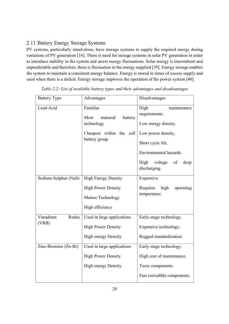
29

2.11 Battery Energy Storage Systems PV systems, particularly stand-alone, have storage systems to supply the required energy during variations of PV generation [16]. There is need for storage systems in solar PV generation in order to introduce stability in the system and arrest energy fluctuations. Solar energy is intermittent and unpredictable and therefore, there is fluctuation in the energy supplied [39]. Energy storage enables the system to maintain a consistent energy balance. Energy is stored in times of excess supply and used when there is a deficit. Energy storage improves the operation of the power system [40].

Table 2.2: List of available battery types and their advantages and disadvantages Battery Type Advantages Disadvantages Lead-Acid Familiar

Most matured battery technology Cheapest within the cell battery group

High maintenance requirements. Low energy density. Low power density. Short cycle life. Environmental hazards. High voltage of deep discharging.

Sodium-Sulphur (NaS) High Energy Density High Power Density Mature Technology High efficiency

Expensive Requires high operating temperature.

Vanadium Redax (VRB)

Used in large applications High Power Density High energy Density

Early-stage technology. Expensive technology. Rugged standardization

Zinc-Bromine (Zn-Br) Used in large applications High Power Density High energy Density

Early-stage technology. High cost of maintenance. Toxic components. Fast corrodible components.

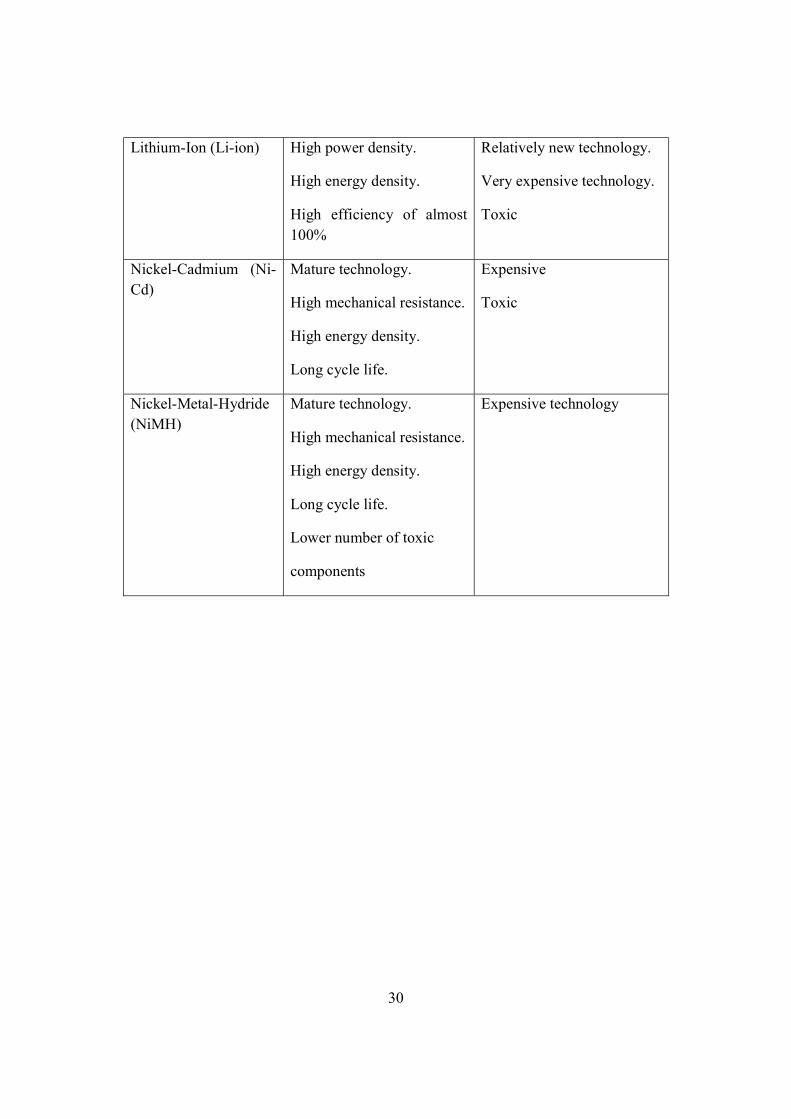
30

Lithium-Ion (Li-ion) High power density. High energy density. High efficiency of almost 100%

Relatively new technology. Very expensive technology. Toxic

Nickel-Cadmium (Ni-Cd)

Mature technology. High mechanical resistance. High energy density. Long cycle life.

Expensive Toxic

Nickel-Metal-Hydride (NiMH)

Mature technology. High mechanical resistance. High energy density. Long cycle life. Lower number of toxic components

Expensive technology

31

3 Development of Devices and Network Models in PSCAD This chapter discusses the development of the network models and device models in PSCAD software environment. 3.1 PSCAD Simulation Software Power Systems Computer Aided Design ( ®) is the simulation software used in the thesis/study. It is developed by Manitoba HVDC Research Centre, a division of Manitoba Hydro International Ltd. PSCAD is a graphical user interface to the Electromagnetic Transients including DC (EMTDC) electromagnetic transient simulation engine [41]. It is a powerful tool that enables the user to schematically construct a circuit, run a simulation, analyze the results, and manage the data in a completely integrated, graphical environment. It further has online plotting functions, controls and meters, which enable the user to alter system parameters while running a simulation. The effects of this alteration can be viewed while the simulation is in progress. It has a comprehensive library of pre-programmed and tested simulation models, which comprise simple passive elements and control functions, more complex models, such as electric machines, full-on FACTS devices, transmission lines and cables. Custom models can be built for models that do not exist. These may be constructed by putting together existing models to form a module, or by constructing models from scratch in a flexible design environment. The study is carried out on two networks: the CIGRE LV network and a typical MV network in Sweden. 3.2 CIGRE Network The CIGRE network is a European LV distribution network benchmark. It is a 20/0.4 kV distribution system fed from a 400 kVA, 20/0.4 kV transformer. Solar PV, wind energy and BESS are integrated into the system. Solar PV is put into the system at nodes C and D rated 3 kW and 4 kW respectively, while BESS is at nodes A and B rated 35 kVA and 25 kVA respectively. They are interfaced to the grid through DC-AC inverters. A wind turbine rated 5.5 kW is at node E. There are loads at nodes C, D, E, R11 and R17. These loads are unbalanced. This network is modelled using PSCAD simulation software using data from [42]. Figure 3.1 shows a single line diagram of the CIGRE network. The description of the model is given in the following section.

32

Figure 3.1: CIGRE LV distribution network 3.3 Model of the CIGRE Network in PSCAD This section describes the modelling of the different components of the network. In addition to the general network components, models were built for the solar photovoltaic system, wind generating system and battery energy storage. The approach taken in building the different models is described in the following sections. 3.3.1 Network Components A three phase, 20kV ideal voltage source is used to represent the grid and a 20/0.4 kV transformer is used to step down the voltage to 400V. The cables between the various nodes (connection points) are represented using pie sections. The parameters are as shown in appendix A. PSCAD has pie section modules and various line parameters can be adjusted using a drop down menu shown in Figure 3.2. The capacitances are not included in the original network due to the short lengths of the cables, however, in this network, PSCAD default capacitance values are used.

0.4kV

R1

Load Bus

Plate

Y

20kV

R0

D

Solar PV

RBatteries A R1

R9

R

Wind Turbine E

R

R C

B Batteries

Solar PV

33

Figure 3.2: Pie section drop down menu

3.3.2 Inverter Modelling in PSCAD Solar PV and BESS are connected to the system using a DC-AC inverter. The inverter topology is the same for all systems in this model. Figure 3.3 shows the basic inverter topology used. It is a three phase inverter which has six switches that are used to chop the direct current (DC) voltage.

Figure 3.3: Inverter topology

The switches used in the inverter are IGBT’s due to their quick switching speed. A snubber circuit is connected in parallel with the switch which helps to suppress large voltage spikes from being imposed across the switch. The values for the snubber resistance and capacitance are the default values in PSCAD. An anti-parallel diode across the switch conducts current when the voltage reverses across the switch. This was used to convert the PV array output from direct current (DC) form to the alternating current (AC) form to be able to tie the PV system to the utility grid. In the

Epv

6.0 [mF]

25.0

1000.0

T

GG

T

+

EnbEna

EnbEna

EncEnbEna

Ia

IGBT4

IGBT1

IGBT6

IGBT3

IGBT2

IGBT5

A CB

22

26

24

21

23

25

Vdc1Vpv

34

PSCAD model, the inverter consist of the Firing Pulse Generator and the Three Phase Inverter Bridge. The signals IGBT1, IGBT2, etc. shown in the inverter schematic in Figure 3.3 are IGBT gate signals which are generated by the Pulse Width Modulation (PWM) circuit. The PWM signals are used to turn the switches on and off to create the desired output. Three sine waves which are used as reference signals are created by the sine function block as depicted in Figure 3.4. After creating these references, they are compared with a 1 kHz triangular carrier wave in a driving block which will finally turn the IGBTs on and off depending upon whether is greater or lesser than (Figure 3.5).

Figure 3.4: Sine reference generation circuit in PSCAD

Figure 3.5: Firing pulse generator

3.3.3 Filter Modelling The AC being injected by the inverter into the grid is not purely sinusoidal due to its high content of harmonics. Therefore, there is need to include a low pass filter that will filter out these harmonics in order to have a high quality AC into the grid. It is advantageous to use a high switching frequency

SinPhase

Phase

FreqMag Sin

RefSigA RefSigB RefSigcRefA RefB RefC

ma

Freq

ma

D +F

+-120.0

Phase

FreqMag Sin

Phase

FreqMag Sin

D +F

+-120.0

IGBT2IGBT5IGBT6IGBT3IGBT4IGBT1Tri

RefCRefCTri

RefCTriTri

RefC

TriRefBRefBTri

RefBTriTri

RefB

TriRefARefATri

RefATriTri

RefA

LH

HL

ON

OFF

LH

HL

ON

OFF

LH

HL

ON

OFF

LH

HL

ON

OFF

LH

HL

ON

OFF

LH

HL

ON

OFF

35

in PWM because the harmonic content of the unfiltered signal occurs around the switching frequency, which is usually much higher than the fundamental. This makes it possible to use smaller filters. The PWM inverter in this model is designed to have a carrier frequency of 1 kHz and a fundamental frequency of 50 Hz. The chosen values for the inductor and capacitor for the LC filter are 200 uH and 7 mF respectively. The LC line filter is shown in Figure 3.6.

Figure 3.6: LC Line filter in PCAD

3.3.4 Solar Photovoltaic System Two solar PV systems are designed, rated 3 and 4 kVA. They use the same inverter topology as described in section 3.3.2. The solar PV array is built using the PV source generator in PSCAD. In the PSCAD master library, there is an inbuilt model of a solar panel component. The solar panel model has the necessary PV cell characteristics. The model is shown in Figure 3.7. When the component parameter menu is open, the user can adjust the PV cell and PV array properties. This is done by selecting drop down menus shown in Figure 3.8.

Figure 3.7: PV solar panel component in PSCAD

C1

B1

A1

Eca1

Ebc1

Eab1200 [uH]

200 [uH]

200 [uH]

7.0 [mF]

7.0 [mF]

7.0 [mF]Eca

Ebc

Eab

C

B

A

G T

+

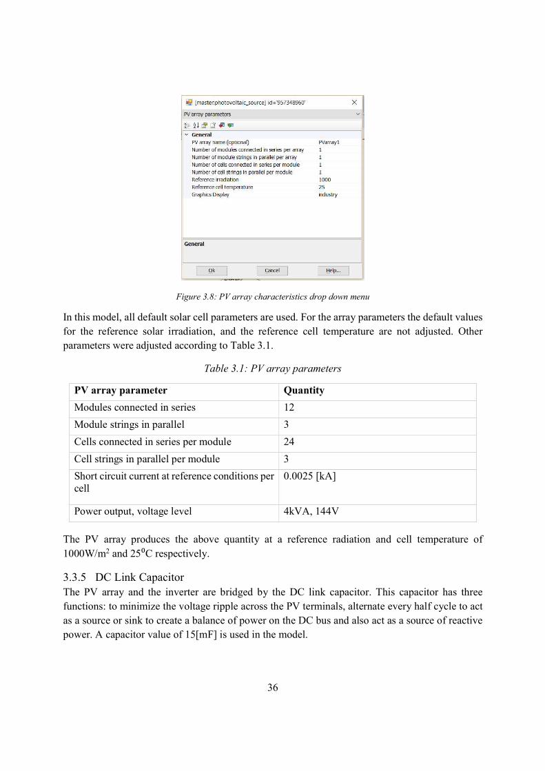
36

Figure 3.8: PV array characteristics drop down menu

In this model, all default solar cell parameters are used. For the array parameters the default values for the reference solar irradiation, and the reference cell temperature are not adjusted. Other parameters were adjusted according to Table 3.1.

Table 3.1: PV array parameters PV array parameter Quantity Modules connected in series 12 Module strings in parallel 3 Cells connected in series per module 24 Cell strings in parallel per module 3 Short circuit current at reference conditions per cell

0.0025 [kA]

Power output, voltage level 4kVA, 144V The PV array produces the above quantity at a reference radiation and cell temperature of 1000W/m2 and 25⁰C respectively. 3.3.5 DC Link Capacitor The PV array and the inverter are bridged by the DC link capacitor. This capacitor has three functions: to minimize the voltage ripple across the PV terminals, alternate every half cycle to act as a source or sink to create a balance of power on the DC bus and also act as a source of reactive power. A capacitor value of 15[mF] is used in the model.

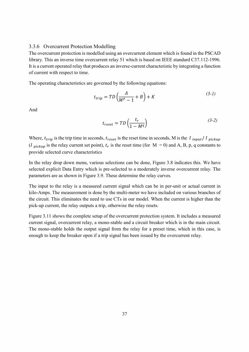
37

3.3.6 Overcurrent Protection Modelling The overcurrent protection is modelled using an overcurrent element which is found in the PSCAD library. This an inverse time overcurrent relay 51 which is based on IEEE standard C37.112-1996. It is a current operated relay that produces an inverse-current characteristic by integrating a function of current with respect to time. The operating characteristics are governed by the following equations: = − 1 + + (3-1)

And = 1 − (3-2)

Where, is the trip time in seconds, is the reset time in seconds, M is the / ( is the relay current set point), is the reset time (for M = 0) and A, B, p, q constants to provide selected curve characteristics In the relay drop down menu, various selections can be done, Figure 3.8 indicates this. We have selected explicit Data Entry which is pre-selected to a moderately inverse overcurrent relay. The parameters are as shown in Figure 3.9. These determine the relay curves. The input to the relay is a measured current signal which can be in per-unit or actual current in kilo-Amps. The measurement is done by the multi-meter we have included on various branches of the circuit. This eliminates the need to use CTs in our model. When the current is higher than the pick-up current, the relay outputs a trip, otherwise the relay resets. Figure 3.11 shows the complete setup of the overcurrent protection system. It includes a measured current signal, overcurrent relay, a mono-stable and a circuit breaker which is in the main circuit. The mono-stable holds the output signal from the relay for a preset time, which in this case, is enough to keep the breaker open if a trip signal has been issued by the overcurrent relay.

38

Figure 3.9: Relay Characteristic Figure 3.10: Relay Menu

Figure 3.11: Overcurrent protection arrangement

In order for the relay to operate as expected, under its settings, values of pickup current and time dial settings are entered. Pick up current throughout the system was initially set to 200% of the full load current. Time dial settings were input as the actual operating time of the protection system. All primary protection was set to operate after 0.04 seconds after the fault. Subsequent protection operated 0.3 seconds later if the primary protection failed. There is also a control algorithm that is implemented to control the operational status of the breakers. Figure 3.12 shows the complete CIGRE low voltage network in PSCAD including distributed generation (DG).

51BRK_L15

I15

Mono-

Tstable

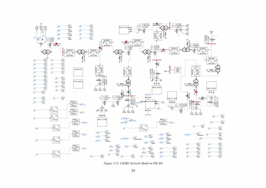
39

Figure 3.12: CIGRE Network Model in PSCAD

#1 #2

R1

#1 #2

80.0 [

ohm]

COUPLEDPISECTION

COUPLEDPI

SECTION

R11

P+jQ P+jQP+jQ

#1 #2

80.0 [

ohm]

R15

COUPLEDPI

SECTION#1

#2

P+jQP+jQP+jQ

80.0 [

ohm]

80.0 [ohm]

#1 #2

R16

#1 #2

80.0 [ohm] P+jQ

P+jQ

A

#1 #2

80.0 [

ohm]

P+jQ

#1#2

COUPLEDPI

SECTION#1

#2

R18

R10

80.0 [ohm]

80.0 [ohm]

P+jQP+jQP+jQ

P = -6.327e-012Q = 1.673e-011V = 0.0001986

V A

P = 0.03231Q = 0.0215V = 0.3984

VA

ABC R=0VaVbVc BinCin

P+jQP = 0.01486Q = 0.009484V = 0.3865

VA

P16Q16V16I16

P16Q16V16I16

P = 0.

006363

Q = 0.

003991

V = 0.

3864

VA

P17

Q17V17

I17

P17

Q17V17

I17

P = 0.

006296

Q = 0.

004063

V = 0.

3848

VA

P18Q18V18I18

P18Q18V18I18

I15V15Q15P15

I15V15Q15P15

P = 0.004266Q = 0.002608V = 0.3929

V A

I11V11Q11P11

I11V11Q11P11

PgridQgridVgridIgrid

PgridQgridVgridIgrid

P = 0.02777Q = 0.0181V = 0.3917

VA

IL3VL3QL3PL3

IL3VL3QL3PL3

P = 0.02766Q = 0.01775V = 0.3873

VA

PL2QL2VL2IL2

PL2QL2VL2IL2

P = 0.01272Q = 0.008094V = 0.3867

VA

IL1VL1QL1PL1

IL1VL1QL1PL1

ABC->GTimedFaultLogic

fl

fl

R17

COUP

LED PISEC

TION

COUPLEDPISECTION

COUPLEDPISECTION

COUPLEDPISECTION

COUPLEDPISECTION

COUPLEDPISECTION

COUPLEDPISECTION

Mono-

Tstable

Igrid

BRK_grid51

Mono-

Tstable

IL3

BRK_L351

Mono-

Tstable

IL2

BRK_L251

Mono-

Tstable

I1851

Mono-

Tstable

IL1

BRK_L151

BRK_L18BRK

_L3

BRK_L2BRK_grid

BRK_L1

BRK_L18

W ind_TurbineAwtBwtCwt

CwtBwtAwt

P = 3.076Q = 7.192e-012V = 0.4967

VA

BESS_35kVAAb Bb Cb

P = 3.

124e-0

07Q =

-2.23

7e-007

V = 0.

6611

VA

Ab Bb Cb

BESS_35kVAAbBbCb

P = 2.152e-007Q = 1.228e-007

V = 0.6611

V A

P = -2.841e-008Q = -1.617e-008V = 0.1173

VA

Solar_PV_3kWAs3Bs3Cs3

P = 4.42e-007Q = -2.387e-007V = 0.7987

VA

Fault_Graphs

Waveforms

VbessrmsVbessrms

IwtQ22

IwtQ22

Vpv4iIpv4

Vpv4iIpv4

Qgrid

Pgrid

Qgrid

PgridVinst Vinst

Ppv4Qpv4Vpv4

Ppv4Qpv4Vpv4

VbessVbessVsrms Vsrms

Vbess25kWVbess25kW Qs3kWPs3kW

Vs3kW

Qs3kWPs3kW

Vs3kW

Qbess1Pbess1Vbess1

Qbess1Pbess1Vbess1

Qwt

Pwt

Qwt

Pwt

IinsIins

Solar_PV_4kW As4Bs4Cs4

Vwti Vwti

Vgrid Vgrid

BRK_3k

WBRK_3kW

Control_blockBRK_WTBRK_3kW

BRK_1BRK_2

BRK_4kW

BRK_1

BRK_4kW

BRK_2

BRK_WT

BRK_s4kW

BRK_W

T

BRK_2

BRK_1

P+jQ

P = 2.461e-007Q = 7.192e-012V = 0.4967

VA

Vwt VwtP22 P22 V22 V22

BRK_L1

551

BRK_L15

I15

Mono-

Tstable

BRK_4kWBRK_s4kW

BRK_L15

40

3.4 Typical Medium Voltage Network in Sweden The MV network used here is supplied from a 20kV substation and contains 30 buses. 13 buses were used in this study due to limitation of the number of electrical nodes in the version of PSCAD used. For purposes of this study, arbitrary three phase loads were added at different buses as shown in Figure 3.13. The PV system was added at bus A. Initial capacity of solar PV system was 4kW but this was gradually increased to determine the level that disrupts the proper functioning of the protection system from that without the distributed generation. A schematic diagram of the network used is shown in the Figure 3.13 below. Using given data in appendix B and the arbitrary loads, the network was modelled in PSCAD as shown in Figure 3.14. Due to limited number of nods we have in the software used, the extent of the model is up to bus X only. The actual network has more buses.

Figure 3.13: Typical MV network

3.4.1 Model of the typical Medium Voltage Network in PSCAD All system components were modelled as described in section 3.3 for the CIGRE network. Cables were modelled using pie sections with values of section lengths, resistances and reactance as shown in Table B. 1 in the Appendix. The default capacitive reactance values were used as they were assumed to have negligible effect on the overall reactance. The solar PV, battery energy storage, dc link capacitor, inverter, filter and protection system were modelled as in the CIGRE network to output values suitable for the MV system.

41

Figure 3.14: Typical MV network as modelled in PSCAD

R=0A

ABAC

COUPLEDPISECTION

COUPLEDPISECTION

COUPLEDPISECTION

EH

X

P = 5.677Q = 1.607V = 22.04

VA

VgridIgridP = 0.04778Q = 0.02101V = 0.001143

VA

P = 0.006185Q = 2.399e-006V = 0.0005008

VA

VgridIgrid

IacIab

IacIab

P = 5.532Q = 1.492V = 21.99

V A

P = 0.9649Q = 0.2606V = 21.92

VA

IeId

IeId

IhIaa

IhIaa

H_XA1B1C1

A2B2C2

P = 0.3039Q = 3.543e-014V = 8.083

VA

IxIx

P+jQ

P+jQP+jQ

P+jQ

IaIaP = 0.00306Q = 0.001947V = 21.99

VA

BRK_S

BRK_STIME

IcIpv

IcIpv

Graphs

Mono-

Tstable

Ia

BRK_A51

ABC->GTimedFaultLogic

fl

BRK_grid

TIME BRK_grid

BRK_A

c

D

COUPLEDPI

SECTION

B

COUPLEDPI

SECTION

COUPLEDPI

SECTION

E_ZA2B2C2

A1B1C1

Z

P+jQ

COUPLEDPISECTION AA

COUPLEDPISECTION

COUPLEDPISECTION G

FCOUPLED

PISECTION

G_HA1B1C1

A2B2C2

BRK_H

P = 0.608Q = 2.534e-014V = 8.084

VA

COUPLEDPISECTION

P = 5.523Q = 1.488V = 21.95

V A

IbIb

P = 4.532Q = 1.239V = 21.93

V A

BRK_B

BRK_E

BRK_F

BRK_C

BRK_D

P = 3.546Q = 0.9911V = 21.93

V A

P = 2.559Q = 0.743V = 21.92

V A

P = 0.6082Q = 0.2347V = 21.91

VA

P = 0.6084Q = 0.2347V = 21.91

VA

BRK_X

BRK_G

BRK_AA

BRK_Z

P = 0.9484Q = 0.2515V = 21.53

VA

IzIg

IzIgIf

IxIfIx

Control_block_1BRK_BBRK_C

BRK_D

BRK_E

Control_block_3BRK_XBRK_Z

BRK_AAControl_block_2BRK_F

BRK_GBRK_H

BRK_K

BRK_H

BRK_G

BRK_F

BRK_K

BRK_D

BRK_C

BRK_B

BRK_E

BRK_AA

BRK_Z

BRK_X

P+jQ

P+jQ

P+jQ

P+jQ

flPVA

BC

BRK_gsP = 0.001485Q = 0.0008896V = 21.99

VA BRK_gs

0.8

Vgs

AB Compar-ator

Undervoltage_sig

pu_pcc_vltg

Undervoltage_sig

BRK_AB

51BRK_AB

Iab

Mono-

Tstable

pv

N

DN/D

22.0 Inverter_disable

1.0 BRK_gs

Inverter_disable

[Main] pv

BRK_gs

BRK_AB

Protection

Ppv Ppv

pu_pcc_vltg

Vpv VpvVpv_instVpv_inst

-sTe

-sTe

Vf

Ph

Frequency andIncremental Phase

Measurement

fi

fifi

Main : Graphs

sT

AB Compar-ator

1.0

AB Compar-ator-1.0

fi

f2 f2

f3 f3

f2

f3

Mono-

Tstable

Mono-

Tstable

ROCOF_prot

42

43

4 Impacts of PV on distribution system protection This chapter discusses the study cases, simulation set ups and results of the simulations. It also presents the impacts of PV on distribution system protection after analyzing the results. 4.1 Description of case studies

Figure 4.1: Methodology of study

After the system was modelled, studies were carried out to ascertain the impacts that solar PV imposes on protection coordination in a distribution network. In the studies, the methodology adopted was to simulate two different cases and compare the results. The first case was simulation without any solar PV integrated, the second case was simulation with solar PV integrated. The results obtained were then analyzed by comparing the two cases. In this instance, fault current levels, fault current directions, and nuisance tripping were examined. The discrepancies between the two cases show the impacts that are as a result of integration of solar PV into the distribution grid.

44

After examining the results, solutions are proposed and simulations were carried out again to see if the impacts have been mitigated by these. 4.2 Simulation Setups Simulations for both the CIGRE and a typical MV networks are carried out. The simulations were first of all done without any solar PV added to get the load currents. Three phase to ground faults were simulated to study the fault current levels. Solar PV was then added to the circuit and then similar faults were simulated and various fault currents recorded. 4.3 CIGRE Network Simulations

Figure 4.2: CIGRE Network Upstream Faults

Figure 4.3: CIGRE Network Downstream Faults

P5 R3

Circuit Breaker

0.4kV

B1

Load Bus

Plate Plate

Y

20kV

B0

D

Solar PV

P3 A R1

7

P4 P2

E

P1

B11 C

B R1

R4

R2

Fault

P5 R3

Circuit Breaker

0.4kV

B1

Load Bus

Plate

Y

20kV

B0

D

Solar PV

P3 A R1

7

P4 P2

E

P1

B11 C

B R1

R4

R2

Fault

45

The simulations on the CIGRE network were carried out according to the following cases: 4.3.1 CIGRE Network Base Case: No PV This simulation was done according to Figure 4-1 and Figure 4-2. The PV was not connected. The procedure is as follows:

Run the simulation without solar PV Simulate three phase to ground faults at buses C, R17, D, E and B11 respectively Record fault currents at the different buses Determine whether or not R3 trips

4.3.2 Results and discussion of the Simulation Table 4.1: Base Case Simulation Results for CIGRE Network

Fault Location Location Fault Current (kA) R3 Trips(Yes/No) C C 0.647 - Line P3-P4 0.665 - Line P2-P3 (R3) 0.66 Yes Line B1-P1 0.674 - R1 0.678 - R17 Line P4-R17 0.914 - Line P3-P4 0.913 - Line P2-P3 (R3) 0.919 Yes Line B1-P1 0.929 - R1 0.934 - D Line P3-D 0.947 - Line P3-P4 N/A - Line P2-P3(R3) 0.95 Yes Line B1-P1 0.962 - R1 0.965 - E Line P2-E (R2) 1.138 - Line P3-P4 N/A - Line P2-P3(R3) N/A No Line B1-P1 1.153 - R1 1.157 - B11 Line P1-B11 1.808 - Line P3-P4 N/A - Line P2-P3(R3) N/A No Line B1-P1 N/A - R1 1.842 -

From table Table 4.1 above, for upstream faults at buses B11 and E, the relay did not issue a tripping command, this is the expected operation of the protection.

46

4.3.3 Simulations with PV connected The aim is to ascertain whether R3 would mal-operate to give a nuisance tripping for upstream faults. This simulation is according Figure 4-2 and Figure 4-3. Solar PV is connected at bus D. The PCC being at P3.

Connect solar PV to the system Run the simulation. Initiate a three phase to ground fault on the upstream. Record fault currents Observe if R3 responds to the fault by tripping the breaker.

4.3.4 Results and discussion of the simulation

Table 4.2: CIGRE Network Upstream Fault Results Fault Location Location Fault Current (kA) R3 Trips(Yes/No)

C C 0.645 - Line P3-P4 0.638 - Line P2-P3 (R3) 0.66 Yes Line B1-P1 0.675 - R1 0.681 - R17 Line P4-R17 0.926 - Line P3-P4 0.909 - Line P2-P3 (R3) 0.916 Yes Line B1-P1 0.928 - R1 0.959 - D Line P3-D 0.953 - Line P3-P4 0.006 - Line P2-P3(R3) 0.946 Yes Line B1-P1 0.959 - R1 0.961 - E Line P2-E (R2) 1.159 - Line P3-P4 N/A - Line P2-P3(R3) 0.418 Yes Line B1-P1 0.76 - R1 0.762 - B11 Line P1-B11 1.826 - Line P3-P4 N/A - Line P2-P3(R3) 0.38 Yes Line B1-P1 0.37 - R1 1.492 -

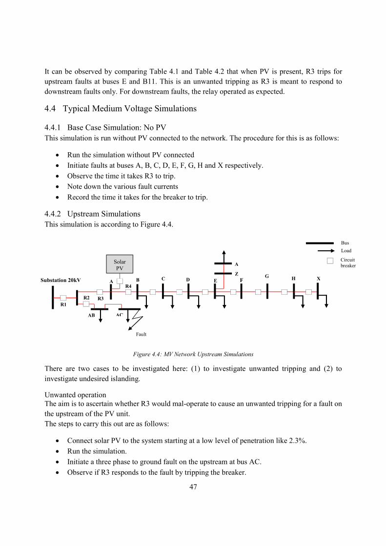
47

It can be observed by comparing Table 4.1 and Table 4.2 that when PV is present, R3 trips for upstream faults at buses E and B11. This is an unwanted tripping as R3 is meant to respond to downstream faults only. For downstream faults, the relay operated as expected. 4.4 Typical Medium Voltage Simulations 4.4.1 Base Case Simulation: No PV This simulation is run without PV connected to the network. The procedure for this is as follows:

Run the simulation without PV connected Initiate faults at buses A, B, C, D, E, F, G, H and X respectively. Observe the time it takes R3 to trip. Note down the various fault currents Record the time it takes for the breaker to trip.

4.4.2 Upstream Simulations This simulation is according to Figure 4.4.

Figure 4.4: MV Network Upstream Simulations There are two cases to be investigated here: (1) to investigate unwanted tripping and (2) to investigate undesired islanding. Unwanted operation The aim is to ascertain whether R3 would mal-operate to cause an unwanted tripping for a fault on the upstream of the PV unit. The steps to carry this out are as follows:

Connect solar PV to the system starting at a low level of penetration like 2.3%. Run the simulation. Initiate a three phase to ground fault on the upstream at bus AC. Observe if R3 responds to the fault by tripping the breaker.

A B C D E F G H Z A

Substation 20kV

AB AC

X

Solar PV

Load Bus

Circuit breaker

Fault

R3 R4

R2 R1

48

If not, increase the level of PV penetration and observe. Note down the level at which R3 will eventually trip. For a nuisance tripping, similar steps are taken but there is no fault initiation carried out.

Undesired islanding The aim is to investigate whether or not the PV unit would island or continue feeding into the fault in the event that R2 fails to operate and R1 operates. If the relay at 3 trips, we would have undesired islanding for the PV generator. 4.4.3 Downstream Fault simulations Figure 4-5 defines the scenario for the simulation with the downstream faults. Two cases are investigated in this scenario, low fault current contribution by PV and high fault contribution by PV.

Figure 4.5: MV Network Downstream Simulations

Low Fault Current Contribution The aim is to determine the effect that increased levels of solar PV below the hosting capacity have on relay tripping times. The procedure is as follows:

Solar PV is connected at Bus A and initially set at 2.3% penetration level. The penetration level being defined as the power contributed by the PV unit against the maximum power demand of the system.

A three phase to ground fault is initiated at 0.6s on bus X. The time it takes R3 to trip is recorded. Solar PV will be increased in steps until 30% and the procedure above followed. The tripping times recorded with inclusion of solar PV are compared to the trip time without

solar PV. The deviations are recorded as the effect that solar PV has on the overcurrent protection coordination.

A B C D E F G H Z AA

Substation 20kV

AB AC

X

Solar PV

Load Bus

Circuit breaker

Fault

R3

R4

R2 R1

49

High Fault Current Contribution This is a high fault current contribution case where the solar PV penetration is 30% or more. The aim of this case is to determine the hosting capacity. The simulations are done according to Figure 4-4.The following steps are used to achieve the result:

The simulation is then run with solar PV penetration set at 30% (from the point reached at in the previous simulation).

A three phase to ground fault is initiated at 0.6s at bus X. It is noted and recorded whether or not R3 trips for downstream faults. Solar PV penetration is increased until a point where R3 does not trip anymore for

downstream faults. The level just before the protection is blinded is the theoretical hosting capacity as regards

protection. This is the level of PV that can be added before protection is blinded. 4.5 Results and discussions from of the MV network case Results, observations and analysis are presented. Tables Table 4.3 and Table 4.4 show the results that have been obtained in the simulation. The rest of the tables are found in appendix C. Observations and analysis are in the preceding sections. 4.5.1 Base Case: No PV It was observed that the R3 was tripping at 0.748s. The tripping time is therefore 0.148s since the simulation is initiated at 0.6s. 4.5.2 Upstream fault Unwanted operation It is observed from Table 4.3 that R3 trips when the level of solar PV penetration is at about 10% or more. This is because at this level, the PV unit is contributing sufficient fault current above the relay settings. This scenario was not accounted for in the original coordination. The original coordination was for a radial network without solar PV. Undesired Islanding For this simulation, R3 was tripping causing the PV unit to island.

50

Table 4.3: Upstream fault simulations, fault location at bus AC 4.5.3 Downstream fault with high fault current contribution from PV The following observations can be made from this simulation:

From Table 4.4, when the solar PV penetration reaches a level of between 30-40%, it has significant impact on the protection coordination.

The Trip times increase tremendously above 40% penetration.

Power contribution Grid (MW) Solar PV

(MW) Trip (Yes/No) % of solar

penetration 7.375 0.1739 No 2.3 7.319 0.2073 No 2.8 7.169 0.5155 No 6.7 7.083 0.5664 No 7.4 6.866 0.6619 No 8.8 6.994 0.6931 No 9.0 6.934 0.7193 No 9.4 6.901 0.7334 No 9.6 6.925 0.7487 No 9.8 6.835 0.7555 No 9.9 6.916 0.7698 Yes 10.0 6.878 0.7703 Yes 10.1 6.781 0.8103 Yes 10.7 6.772 0.8236 Yes 10.8 6.65 0.9785 Yes 12.8

6.012 1.518 Yes 20.2

51

As shown in Table C.4 at penetrations above 62%, the relay R3 does not trip at all for downstream faults. 62% is the theoretical hosting capacity in this case. The longest tripping time before the relay is blinded to faults on the downstream is about 1.54s after fault initiation.

Figure 4.6: Plot of trip time with and without solar PV up to hosting capacity

Table 4.4: Downstream, high fault current contributions, fault location at bus X Grid power (MW)

Solar PV (MW)

Trip time with solar PV (s)

% of solar penetration

2.2 5.395 Did not trip 71.0 2.42 5.185 Did not trip 68.2

2.469 5.072 Did not trip 67.3 2.737 4.911 Did not trip 64.2 2.892 4.759 1.54 62.2 2.919 4.705 1.413 61.7 3.12 4.511 0.931 59.1

3.936 3.719 0.425 48.6 3.992 3.573 0.416 47.2

52

4.008 3.591 0.413 47.3 4.466 3.19 0.334 41.7 4.971 2.725 0.282 35.4 5.183 2.455 0.263 32.1 5.415 2.262 0.249 29.5 5.675 2.014 0.23 26.2 5.856 1.803 0.23 23.5 6.103 1.541 0.211 20.2 6.444 1.198 0.202 15.7 6.616 0.9723 0.202 12.8 7.023 0.504 0.181 6.7 7.191 0.3416 0.181 4.5 7.508 0.1772 0.181 2.3

4.5.4 Downstream with low fault current contribution from PV The following observations can be made from this simulation:

R3 trips for faults on the downstream and the PV unit islands. The tripping times increase from 0.148s when no PV is connected to maximum 1.54s until

hosting capacity is reached for the case when PV is connected at A. 4.5.5 Variation of fault currents with varying fault locations Figure 4.7 to Figure 4.9 show the variation of fault currents at different locations. It is seen from Figure 4.7 that the grid fault current reduces with connection of solar PV, the further the fault downstream, the lower the fault current contribution from the grid. This reduced fault current causes longer tripping times.

53

Figure 4.7: Variation of grid and fault currents with faults downstream, PCC at A, PV at 30% penetration

Figure 4.8: Variation of grid and fault currents with faults downstream, PCC at E and PV at 30% penetration

0.0010.0020.0030.0040.0050.0060.0070.00

PCC B C D E F G H X

Fault cu

rrent m

agnitud

e (kA)

Fault location

0.0010.0020.0030.0040.0050.0060.0070.00

A B C D E (PCC) F G H X

Fault cu

rrent m

agnitud

e (kA)

Fault location

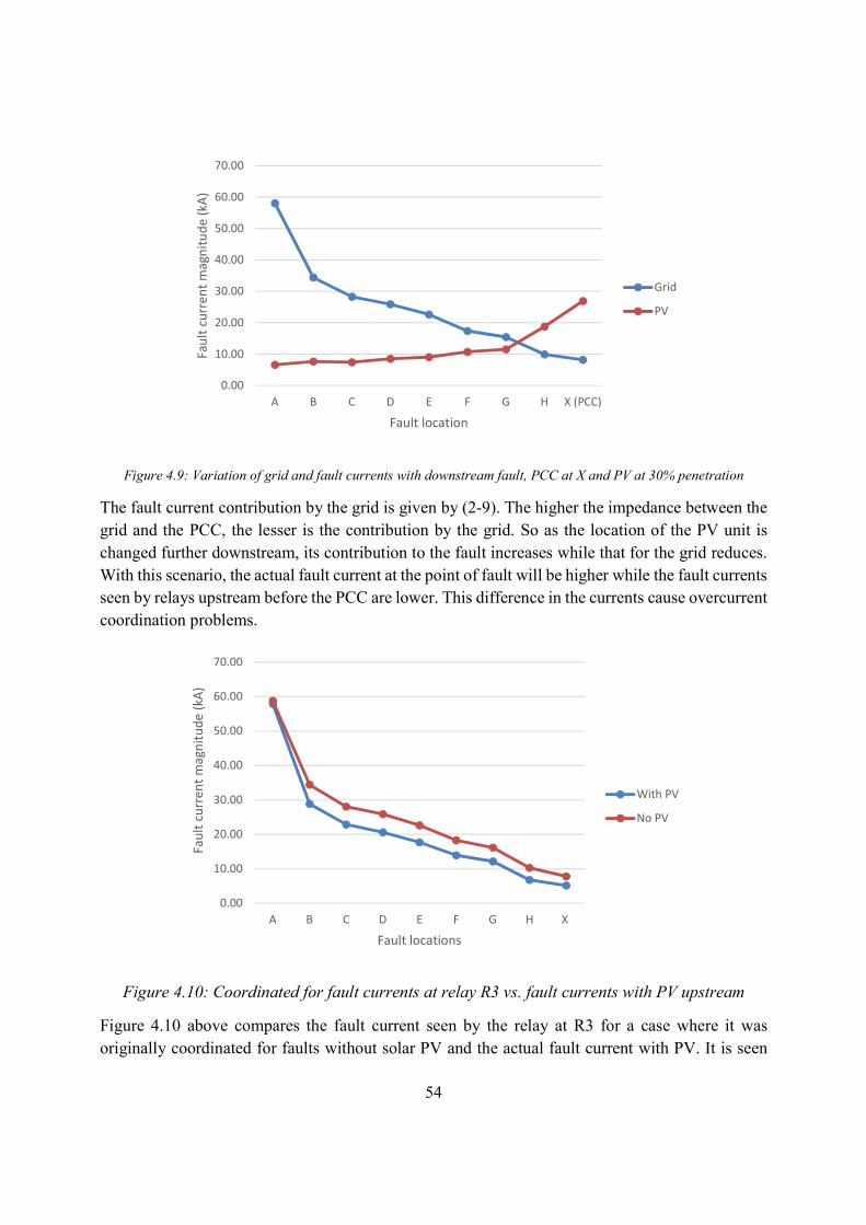
54

Figure 4.9: Variation of grid and fault currents with downstream fault, PCC at X and PV at 30% penetration

The fault current contribution by the grid is given by (2-9). The higher the impedance between the grid and the PCC, the lesser is the contribution by the grid. So as the location of the PV unit is changed further downstream, its contribution to the fault increases while that for the grid reduces. With this scenario, the actual fault current at the point of fault will be higher while the fault currents seen by relays upstream before the PCC are lower. This difference in the currents cause overcurrent coordination problems.

Figure 4.10: Coordinated for fault currents at relay R3 vs. fault currents with PV upstream

Figure 4.10 above compares the fault current seen by the relay at R3 for a case where it was originally coordinated for faults without solar PV and the actual fault current with PV. It is seen

0.0010.0020.0030.0040.0050.0060.0070.00

A B C D E F G H X (PCC)

Fault cu

rrent m

agnitud

e (kA)

Fault location

GridPV

0.0010.0020.0030.0040.0050.0060.0070.00

A B C D E F G H X

Fault cu

rrent m

agnitud

e (kA)

Fault locations

With PVNo PV

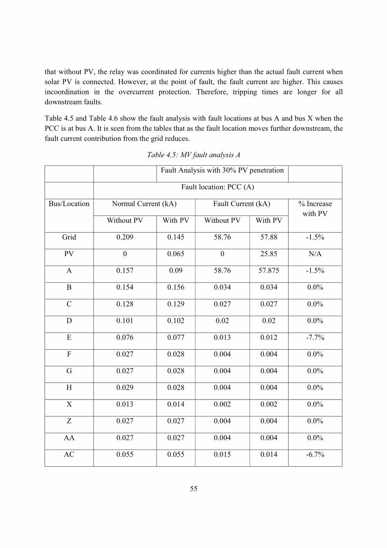
55

that without PV, the relay was coordinated for currents higher than the actual fault current when solar PV is connected. However, at the point of fault, the fault current are higher. This causes incoordination in the overcurrent protection. Therefore, tripping times are longer for all downstream faults. Table 4.5 and Table 4.6 show the fault analysis with fault locations at bus A and bus X when the PCC is at bus A. It is seen from the tables that as the fault location moves further downstream, the fault current contribution from the grid reduces.

Table 4.5: MV fault analysis A Fault Analysis with 30% PV penetration Fault location: PCC (A)

Bus/Location Normal Current (kA) Fault Current (kA) % Increase with PV Without PV With PV Without PV With PV

Grid 0.209 0.145 58.76 57.88 -1.5% PV 0 0.065 0 25.85 N/A A 0.157 0.09 58.76 57.875 -1.5% B 0.154 0.156 0.034 0.034 0.0% C 0.128 0.129 0.027 0.027 0.0% D 0.101 0.102 0.02 0.02 0.0% E 0.076 0.077 0.013 0.012 -7.7% F 0.027 0.028 0.004 0.004 0.0% G 0.027 0.028 0.004 0.004 0.0% H 0.029 0.028 0.004 0.004 0.0% X 0.013 0.014 0.002 0.002 0.0% Z 0.027 0.027 0.004 0.004 0.0%

AA 0.027 0.027 0.004 0.004 0.0% AC 0.055 0.055 0.015 0.014 -6.7%

56

Table 4.6: MV fault analysis, bus X Fault Analysis with 30% PV penetration Fault location: X Bus/Location Normal Current (kA) Fault Current (kA) % Increase with

PV Without PV With PV Without PV With PV Grid 0.209 0.145 8.554 5.461 -36.2% PV 0 0.065 0 4.104 N/A A 0.157 0.09 7.785 5.119 -34.2% B 0.154 0.156 7.904 8.11 2.6% C 0.128 0.129 7.894 8.71 10.3% D 0.101 0.102 7.885 8.7 10.3% E 0.076 0.077 7.877 8.535 8.4% F 0.027 0.028 8.05 9.207 14.4% G 0.027 0.028 8.05 9.207 14.4% H 0.029 0.028 8.067 8.552 6.0% X 0.013 0.014 8.064 8.49 5.3% Z 0.027 0.027 0.021 0.021 0.0%

AA 0.027 0.027 0.021 0.01 -52.4% AC 0.055 0.055 0.05 0.052 4.0%

57

Figure 4.11: Summary of results

4.5.6 Summary of Impacts of Connecting Solar PV to a Distribution Network From results shown in Figure 4.11 the summary for the effects of solar PV to a distribution grid can be summarized as follows:

When there is very little or no impedance between the PCC and the fault point, the coordination holds as seen for the simulations for the CIGRE network.

Increased fault currents at point of fault, Reduced fault currents between the grid and PCC Loss of relay sensitivity Loss of coordination and longer tripping times Undesired tripping for faults on the upstream (With 10% penetration of solar PV) Blinding of protection Unintentional islanding

58

59

5 Solutions to identified problems This chapter presents solutions that mitigate the identified impacts and describe how the chosen solutions perform 5.1 Solutions In order to solve some of the impacts identified above, three solutions are proposed and simulated in this thesis. These are DTT, undervoltage protection and ROCOF. These methods are described in the preceding sections. Figure 5.1, Figure 5.2, Figure 5.3 and Figure 5.4 depict these schemes. 5.1.1 Direct Transfer Trip using wireless link This scheme is used to mitigate the following impacts:

Increased fault current Reduced fault current Unintended islanding Unwanted tripping Reverse fault current Unsynchronized reclosing

This is overcurrent protection which is as described in section 3.3.6, which is meant to trip the upstream breaker (and other breakers meant to provide backup) in the event of a fault. However, the overcurrent protection in this design has capability to communicate with the PV unit downstream in the event of an upstream fault. The communication system is comprised of a delay element and a transmission radio link. There is no delay set in this simulation. This signal can be transmitted through any communication method. In this design, a radio link is used. At the remote end where the PV unit is, this signal is interfaced with other PV protection signals to communicate with the inverter. The signal from the upstream overcurrent protection is received by an interfacing circuit. The description of the interfacing circuit follows in section 5.1.3. The overcurrent protection scheme with communication capability as modelled in PSCAD is shown in Figure 5.1.

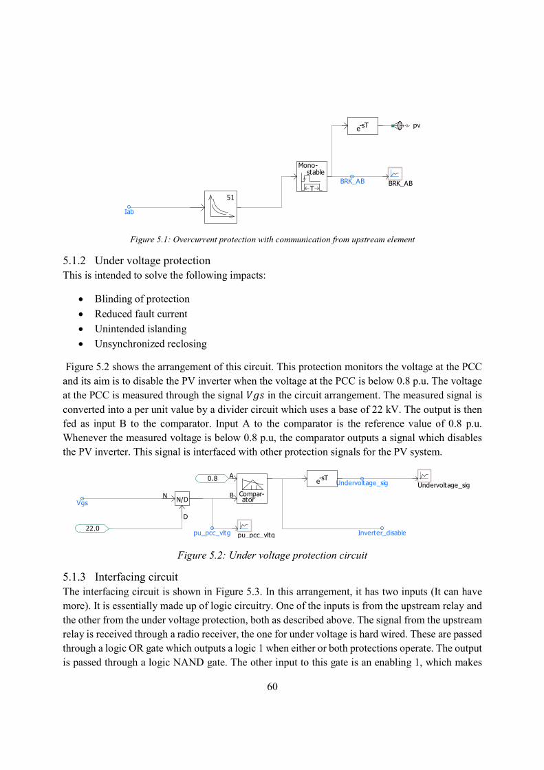
60

Figure 5.1: Overcurrent protection with communication from upstream element

5.1.2 Under voltage protection This is intended to solve the following impacts:

Blinding of protection Reduced fault current Unintended islanding Unsynchronized reclosing

Figure 5.2 shows the arrangement of this circuit. This protection monitors the voltage at the PCC and its aim is to disable the PV inverter when the voltage at the PCC is below 0.8 p.u. The voltage at the PCC is measured through the signal in the circuit arrangement. The measured signal is converted into a per unit value by a divider circuit which uses a base of 22 kV. The output is then fed as input B to the comparator. Input A to the comparator is the reference value of 0.8 p.u. Whenever the measured voltage is below 0.8 p.u, the comparator outputs a signal which disables the PV inverter. This signal is interfaced with other protection signals for the PV system.

Figure 5.2: Under voltage protection circuit

5.1.3 Interfacing circuit The interfacing circuit is shown in Figure 5.3. In this arrangement, it has two inputs (It can have more). It is essentially made up of logic circuitry. One of the inputs is from the upstream relay and the other from the under voltage protection, both as described above. The signal from the upstream relay is received through a radio receiver, the one for under voltage is hard wired. These are passed through a logic OR gate which outputs a logic 1 when either or both protections operate. The output is passed through a logic NAND gate. The other input to this gate is an enabling 1, which makes

51BRK_AB

Iab

Mono-

Tstable

pv

BRK_AB

-sTe

0.8

Vgs

AB Compar-ator

Undervoltage_sig

pu_pcc_vltg

Undervoltage_sigN

DN/D

22.0 Inverter_disablepu_pcc_vltg

-sTe

61

the output of this gate dependent upon the protection signal only. Table 5.1 shows the truth table for this NAND gate.

Table 5.1: NAND gate truth table Enabling

Signal Protection Output

0 0 X 0 1 X 1 0 1 1 1 0

The interfacing circuit output is dependent upon the protection signal. When there is no fault in the system, there is no signal from the protection and hence the output of the interfacing circuit is a logic 1. When the protection operates, the output of the interfacing circuit is a logic 0. This output is then fed to the firing pulse circuit which is described in the following section.

Figure 5.3: Protection interfacing circuit

5.1.4 Firing pulse circuit with protection disabling signal Figure 5.4 shows the inverter firing pulse circuit. The operation of the inverter was described in section 3.3.1. It is modified here such that AND logic gates are included on the outputs of the pulse driving circuits. These are meant to combine the protection signal and the firing pulses from the pulse driving circuits. The output from the AND gate are now the pulses that provide the firing to the IGBTs in the PV inverter circuit. The truth table that governs the output for the circuit is shown in Table 5.2.

1.0 BRK_gs

Inverter_disable

[Main] pv

BRK_gsProtect ion

62

Table 5.2: Truth table for AND gate Firing pulse

Protection Output

0 0 0 0 1 0 1 0 0 1 1 1

The inverter has two modes, normal operating mode and blocking mode. These two modes are decided by the protection. When the protection has not operated, the inverter is in the normal operating mode. When the protection has operated, the inverter is in blocked mode and it does not produce any output. Under normal operation, the firing pulse circuit will drive the inverter IGBTs only when the firing pulse circuit is firing and the interfacing is supplying a logic 1 signal, that is, when the protection has not operated. Without a fault in the system, the interfacing circuit always has a logic 1, meaning the inverter is always enabled. It’s functioning entirely depends upon the pulse firing circuit. When the protection circuit operates, the interfacing circuit will output a logic 0. In this situation, whatever the output of the pulse firing circuit, the overall output to the firing circuit will be a logic 0 and the inverter will not chop the DC voltage. The inverter is therefore disabled when the protection has operated.

Figure 5.4: Firing pulse circuit to include protection signal

LH

HL

ON

OFF

LH

HL

ON

OFF

LH

HL

ON

OFF

LH

HL

ON

OFF

LH

HL

ON

OFF

LH

HL

ON

OFFRefATriTri

RefA

TriRefARefATri

RefBTriTri

RefB

TriRefBRefBTri

RefCTriTri

RefC

TriRefCRefCTri

IGBT1 IGBT4 IGBT3 IGBT6 IGBT5 IGBT2Protection

63

5.1.5 Rate of Change of Frequency Protection (ROCOF) This protection is an anti-islanding protection designed to trip the PV unit when it has islanded and the rate of change of frequency is above or below a certain threshold value. It also protects against unsynchronized reclosing. Figure 5.5 and Figure 5.6 illustrate this scheme as implemented in this project in the PSCAD/EMTDC environment.

Figure 5.5: ROCOF signal pickup

Figure 5.6: ROCOF protection

The frequency and its rate of change are measured using the arrangement as shown in Figure 5.5. The signal is then fed to the ROCOF relay. It is comprised of two comparators that enable the relay to protect for both positive and negative rate of change. The output from the comparators, through mono-stables, is fed to a logic OR gate. The output from the OR gate is then passed through a logic AND gate. The other input to the AND gate is a signal from the upstream overcurrent relay. This is an interlock to ensure that the ROCOF protection will only operate when the upstream breaker has tripped and the PV has islanded. Otherwise, it is not supposed to operate. The output from the AND gate is passed through an OR gate. This is for the purpose of interfacing breaker controls whereby the breaker is also operator controlled for the purpose of switching the PV unit on-off. The output from this final OR gate is the signal that controls the PV unit breaker. 5.2 Performance of the proposed solutions The above proposed solutions were simulated and their effectiveness in mitigating the identified impacts were ascertained.

cP = 3.546

Q = 0.9911V = 21.93

V AP+jQV

f

Ph

Frequency andIncremental Phase

Measurement fisT

Mono-

Tstable

Mono-

Tstable

rate_of_change_of_frequency

-1.0

AB Compar-ator

1.0 AB Compar-ator

-sTe

BRK_A TIME

BRK_S

64

5.2.1 Direct Transfer Trip (Overcurrent protection with communication) The following is the sequence by which this protection operates;

A fault occurs in the upstream Overcurrent on the upstream detects the fault A signal is generated which both trips the local breaker and also communicates with the

solar PV This protection signal turns the inverter off The PV unit will no longer contribute to the fault Only the required upstream breakers operate for the fault.

Figure 5.7: Overcurrent protection and Direct Transfer Trip signals

Figure 5.8: Upstream faulty feeder and PV current fault currents

Figure 5.7 and Figure 5.8 show the performance of the DTT scheme. At the occurrence of the fault, the overcurrent protection detects the fault (relay R2 in Figure 4.4). The relay issues a trip command

Main : Graphs

sec 0.580 0.600 0.620 0.640 0.660 0.680 0.700

0.00 0.20 0.40 0.60 0.80 1.00 1.20 DTT_signal BRK_AB

Main : Graphs

sec 0.560 0.580 0.600 0.620 0.640 0.660 0.680 0.700 0.720 0.740 0.760

0

10

20

30

40

50 Ipv Iab

65

to the breaker and also issues a direct transfer trip command to the PV protection system. Figure 5.7 shows these signals as obtained in the simulation. The response to these signals is shown in Figure 5.8. The upstream breaker and the PV unit are tripped at 0.653s, eliminating any chance of relay R3 (in Figure 4.4) responding to trip the breaker, thereby islanding the PV unit. 5.2.2 Under voltage Protection The under voltage protection was simulated for downstream high and low fault current contributions. The measured voltage was obtained from the PCC. Downstream, High fault contribution mitigation As highlighted in section 4.5.3, at PV penetration levels of 62% and above, the overcurrent protection is blinded, it does not operate for faults at bus X. The under voltage protection mitigates this condition. Below is the sequence by which this is effected;

A fault occurs at bus X in this case, with the PV contributing much of the fault current as in Figure 4.9.

The original overcurrent protection does not detect the fault because the PV contributes much to the fault current as compared to the grid.

The fault causes the voltage at the PCC to reduce to below 0.8 pu. This triggers the undervoltage protection.

The under voltage protection disables the PV unit and therefore its contribution to the fault is curtailed.

With the PV unit out of the system, the original overcurrent protection coordination is restored.

When the PV unit is disabled, the whole fault current will now be supplied by the grid. The overcurrent protection will now operate to isolate the original fault.

Figure 5.9: Grid and PV fault currents during fault

Main : Graphs

sec 0.560 0.580 0.600 0.620 0.640 0.660 0.680 0.700 0.720 0.740

0 20 40 60 80

100 120 140 160 Ipv Igrid

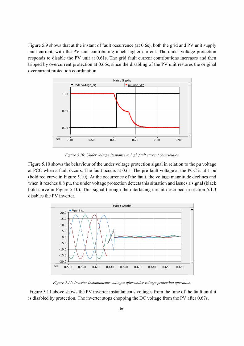
66

Figure 5.9 shows that at the instant of fault occurrence (at 0.6s), both the grid and PV unit supply fault current, with the PV unit contributing much higher current. The under voltage protection responds to disable the PV unit at 0.61s. The grid fault current contributions increases and then tripped by overcurrent protection at 0.66s, since the disabling of the PV unit restores the original overcurrent protection coordination.

Figure 5.10: Under voltage Response to high fault current contribution

Figure 5.10 shows the behaviour of the under voltage protection signal in relation to the pu voltage at PCC when a fault occurs. The fault occurs at 0.6s. The pre-fault voltage at the PCC is at 1 pu (bold red curve in Figure 5.10). At the occurrence of the fault, the voltage magnitude declines and when it reaches 0.8 pu, the under voltage protection detects this situation and issues a signal (black bold curve in Figure 5.10). This signal through the interfacing circuit described in section 5.1.3 disables the PV inverter.

Figure 5.11: Inverter Instantaneous voltages after under voltage protection operation.

Figure 5.11 above shows the PV inverter instantaneous voltages from the time of the fault until it is disabled by protection. The inverter stops chopping the DC voltage from the PV after 0.67s.

Main : Graphs

sec 0.40 0.50 0.60 0.70 0.80 0.90

0.00

0.50

1.00

Undervoltage_sig pu_pcc_vltg

Main : Graphs

sec 0.580 0.590 0.600 0.610 0.620 0.630 0.640 0.650 0.660

-20.0 -15.0 -10.0 -5.0 0.0 5.0

10.0 15.0 20.0 Vpv_inst

67

Downstream Low Fault Current Mitigation This problem as described in section 4.5.4 is mitigated by the under voltage protection. At penetrations of solar PV of above 30%, the overcurrent protection coordination is affected. The protection takes longer to trip and isolate the fault. In this case, the under voltage protection will operate to isolate the fault. The mitigation process is as described for the high fault current scenario above. 5.2.3 ROCOF Protection The protection operates as follows:

A fault occurs on the downstream of the PV unit The overcurrent protection detects this fault and trips the upstream breaker, though with a

delayed response After the upstream breaker is tripped, frequency excursions are experienced due to the

imbalance created now between the PV unit power and the load The tripping of the upstream breaker will release the interlock for the ROCOF protection to

be able to operate If the frequency excursions are above ±1hz/s, the ROCOF protection operates to trip the

PV unit. Figure 5.12 shows the frequency excursions and rate of change of this frequency experienced by the PV system during and after the fault. The fault is initiated at 0.6s. This causes the overcurrent protection to trip the upstream breaker. The tripping signal releases the ROCOF protection interlock, which enables this protection to operate.

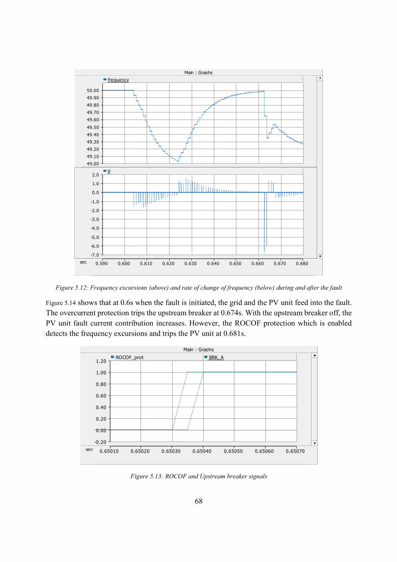
68

Figure 5.12: Frequency excursions (above) and rate of change of frequency (below) during and after the fault

Figure 5.14 shows that at 0.6s when the fault is initiated, the grid and the PV unit feed into the fault. The overcurrent protection trips the upstream breaker at 0.674s. With the upstream breaker off, the PV unit fault current contribution increases. However, the ROCOF protection which is enabled detects the frequency excursions and trips the PV unit at 0.681s.

Figure 5.13: ROCOF and Upstream breaker signals

Main : Graphs

sec 0.590 0.600 0.610 0.620 0.630 0.640 0.650 0.660 0.670 0.680

49.00 49.10 49.20 49.30 49.40 49.50 49.60 49.70 49.80 49.90 50.00

frequency

-7.0 -6.0 -5.0 -4.0 -3.0 -2.0 -1.0 0.0 1.0 2.0 fi

Main : Graphs

sec 0.65010 0.65020 0.65030 0.65040 0.65050 0.65060 0.65070

-0.20 0.00 0.20 0.40 0.60 0.80 1.00 1.20 ROCOF_prot BRK_A

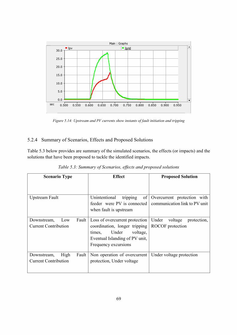
69

Figure 5.14: Upstream and PV currents show instants of fault initiation and tripping

5.2.4 Summary of Scenarios, Effects and Proposed Solutions Table 5.3 below provides are summary of the simulated scenarios, the effects (or impacts) and the solutions that have been proposed to tackle the identified impacts.

Table 5.3: Summary of Scenarios, effects and proposed solutions Scenario Type Effect Proposed Solution

Upstream Fault Unintentional tripping of feeder were PV is connected when fault is upstream

Overcurrent protection with communication link to PV unit

Downstream, Low Fault Current Contribution

Loss of overcurrent protection coordination, longer tripping times, Under voltage, Eventual Islanding of PV unit, Frequency excursions

Under voltage protection, ROCOF protection

Downstream, High Fault Current Contribution

Non operation of overcurrent protection, Under voltage

Under voltage protection

Main : Graphs

sec 0.500 0.550 0.600 0.650 0.700 0.750 0.800 0.850 0.900 0.950

0.0 5.0

10.0 15.0 20.0 25.0 30.0 Ipv Igrid

70

71

6 Conclusions and Future Work This chapter presents the conclusions that have been drawn after building models in PSCAD of the CIGRE low voltage network and a typical medium voltage network and studying the impacts associated with integrating solar on the overcurrent protection of the system. Prospects of future work in this area are also presented in order to fully understand the subject and associated mitigating solutions. 6.1 Conclusions Solar PV is an attractive form of energy that promises energy security with many environmental benefits. However, these benefits cannot be realized fully because integrating solar PV into a traditional radial distribution network poses a number of challenges. This thesis developed distribution models in EMTDC/PSCAD including inverse-time overcurrent protection. Solar PV was added and its impact on overcurrent protection coordination was investigated. These impacts as seen from the simulations, depend upon the location of the PV unit and the penetration level. The location of the fault also determines the type of impact that is experienced by the system. The level of solar penetration at which these impacts manifested for faults on the downstream is about 30% and above, while on the upstream they manifested at about 10%. From the study, the following conclusions can be made:

When solar PV is present in a distribution grid, false tripping of feeders nuisance tripping of protective devices blinding of protection, increase or decrease of fault current levels and unwanted islanding are some of the impacts that are experienced by the grid. These impacts are observed at solar PV penetration levels of 30% or more. Tripping times increase for faults.

Fault current levels increase/decrease. At the point of the fault, fault currents increase due to the fact that all sources are contributing to the fault current, however, on the upstream of the PV unit, the fault currents reduce. This is because the PV unit is now contributing a part of the fault current.

The theoretical hosting capacity in terms of protection was determined to be about 62%. Protection against unintended islanding proved adequate in solving some of the identified

impacts. The following solutions have been found in this thesis to be effective: Direct Transfer Trip, under voltage protection and ROCOF protection.

72

6.2 Future Work The main focus in this thesis was to study the steady state impacts of solar PV on the protection system of the CIGRE and a typical medium voltage distribution networks. In this case, variation of solar insolation was not considered. The study can be extended to look at the following:

Variation in power production by solar. The effects on other protection schemes other than overcurrent protection. Meshed networks with other types of DERs. Optimal location of solar PV

73

References [1] Wikipedia, "Growth of photovoltaics," [Online]. Available:

https://en.wikipedia.org/wiki/Growth_of_photovoltaics. [Accessed 1 June 2016]. [2] Clean Teachnica, "Solar Power," Clean Technica, [Online]. Available:

http://cleantechnica.com/solar-power/. [Accessed 8 2 2016]. [3] Wikipedia, "Growth of photovoltaics," Wikipedia, [Online]. Available:

https://en.wikipedia.org/wiki/Growth_of_photovoltaics. [Accessed 8 2 2016]. [4] International Electrotechnical Commission, Market Strategy Board, "Grid Integration of

large-capacity Renewable Energy sources and use of large capacity Electrical Energy Storage," International Electrotechnical Commision White Paper, Geneva, 2012.

[5] J. P. Lopes, N. Hatziargyriou, J. Mutale, P. Djapic and N. Jenkis, "Integrating distributed generation into electric power systems: A review of drivers, challenges and opportunities," Electric Power Systems Research, vol. 77, no. 9, pp. 1143-1238, 2007.

[6] S. Chowdhury, S. Chowdhury, C. F. Ten and P. A. Crossley, "Islanding Protection of Distribution Systems with Distributed Generators - A comprehensive Survey Report," in Power and Energy Society Meeting - Conversion and Delivery of Electrical Energy in the 21st Century, 2008.

[7] L. Hewitson, M. Brown and B. Ramesh, Practical Power System Protection, Newness , 2004. [8] North American Reliability Corporation, Protection System Maintenance and Testing

Standard Drafting Team, PRC-005-2 Protection - System Maintenance supplementary Reference, Princeton, 2009.

[9] IEEE, IEEE 100, The Authoritative Dictionary of IEEE Standards Terms, Seventh ed., IEEE Press, 2000.

[10] J. M. Gers and E. J. Holmes, Protection of Electricity Distribution Networks, Third ed., The Institution of Engineering and Technology, pp. 61-79.

[11] P. M. Anderson, Power System Protection, IEEE Press, 1999, pp. 201-240, 249-257. [12] [Online]. Available: http://www.electrical4u.com/types-of-electrical-protection-relays-or-

protective-relays. [Accessed 14 April 2016].

74

[13] IEEE, "IEEE Std 242-2001," IEEE buff book, 2001. [14] Joint Working Group B5/C6.26/CIRED, "Protection of Distribution Systems with Distributed

Energy Resources," March 2015. [15] M. C. B. Ravindranath, Power System Protection and Switchgear, New Delhi: New Age

International (P) Ltd., 2005. [16] N. M. Pearsall and R. Hill, "Photovoltaic Modules, Systems and Applications," in Clean

Electricity from Photovoltaics, World Scientific, 2001, pp. 688-689. [17] G. Knier, "NASA Science News," NASA, 2002. [Online]. Available:

http://http://science.nasa.gov/science-news/science-at-nasa/2002/solarcells/. [Accessed 2 February 2016].

[18] C. Honsberg and S. Bowden, "Semiconductor Materials," PVEducation.org, [Online]. Available: http://pveducation.org/pvcdrom/pn-junction/semiconductor-materials. [Accessed 2 February 2016].

[19] "Introduction to Photovoltaics," Solar-Facts, [Online]. Available: http://www.solar-facts.com/panels/. [Accessed 2 February 2016].

[20] M. D. Archer and R. Hill, Clean Electricity from Photovoltaics, World Scientific, 2001. [21] Solar facts, "solar-facts," Solar-Facts, [Online]. Available: http://www.solar-

facts.com/panels/. [Accessed 23 January 2016]. [22] A. Brown, S. Muller and Z. Dobrotkova, "Renewable Energy: Markets and Prospects by

Technology," International Energy Agency Information Paper, 2011. [23] IEEE Standards Coordinating Committee 21 on Fuel Cells, Photovoltaics, Dispersed

Generation, and Energy Storage, IEEE Recommended Practice for Utility Interface of Photovoltaic (PV) Systems, IEEE, 2000.

[24] B. Weller, C. Hemmerle, S. Jakubetz and S. Unnewehr, Photovoltaics: Technology, Architecture, Installation, Basel: Birkhäuser, 2012.

[25] Solar Direct, "Solar Direct," [Online]. Available: http://www.solardirect.com. [Accessed 23 January 2016].

[26] H. Häbelin, Photovoltaics System Design and Practice, Hoboken: John Wiley & Sons, 2012.

75

[27] F. Katiraei and J. R. Aguero, "Solar PV Integration Challenges," IEEE power & energy magazine, no. 63, 2011.

[28] A. Girgis and S. Brahma, "Effect of Distributed Generation on Protective Device Coordination in Distribution System," in Large Engineering Systems Conference, Halifax, NS, 2001.

[29] M. T. Doyle, "Reviewing Impacts of Distributed Generation on Distribution System Protection," in Power Engineering Society Summer Meeting, 2002 IEEE, Chicago, 2002.

[30] H. Zayandehroodi, A. Mohamed, H. Shareef and M. Mohammadjafari, "Impact of distributed generations on power system protection performance," International Journal of Physical Sciences, vol. 6, no. 16, pp. 3999-4007, 2011.

[31] M. Bollen and F. Hassan, Integration of Distributed Generation in the Power System, 1st ed., John Wiley & Sons, Inc., 2011.

[32] CIGRE Task Force, "Benchmark Systems for Network Integration of Renewable and Distributed Energy Resources," CIGRE, Berlin, July 2009.

[33] G. Tang and M. R. Iravani, "Application of a Fault Current Limiter To Minimize Distributed Generation Impact on Coordinated Relay Protection," in International Conference on Power Systems transients (IPST'05), Montreal, Canada, 2005.

[34] Z. Hadi, A. Mohamed, H. Shareef and M. Mohammadjafari, "A Comprehensive review of protection coordination methods in power distribution systems in the presence of DG," Electrical Review, no. 8, 2011.

[35] M. Khederzadeh, "Application of TCSC to Restore Directional Overcurrent Relay Coordination in Systems with Distributed <generation," in 10th International Conference on Electricity Distribution, Prague, June,2009.

[36] S. M. Brahma and A. A. Girgis, "Development of Adaptive Protection Scheme for Distribution Systems With High Penetration of Distributed Generation," in IEEE transactions on Power Delivery, 2004.

[37] H. H. Zeineldin, H. M. Sharaf, D. K. Ibrahim and E. E.-D. A. El-Zahab, "Optimal Protection Coordination for Meshed Distribution Systems With DG Using Dual Setting Directional Over-current Relays," IEEE Transactions on Smart Grid, vol. 6, no. 1, pp. 115-123, January 2015.

76

[38] A. Ukil, B. Deck and V. H. Shah, "Smart Distribution Protection using Current-Only Directional Overcurrent Relay".

[39] G. Coppez, S. Chowdhury and S. P. Chowdhury, "The Importance of Energy Storage in Renewable Power Generation: A Review," in Universities Power Engineering Conference (UPEC), 45th International, Cardiff, 2010.

[40] J. Paska, P. Biczel and M. Klos, "Technical and Economic Aspects of Electricity Storage Systems Co-operating with Renewable Energy Sources," in Electrical Power Quality and Utilization, 2009. EPQU 2009. 10th International Conference, Lodz, 2009.

[41] Manitoba HVDC Research Centre, User's Guide on the use of PSCAD, Manitoba Hydro International Limited, 2010.

[42] "Benchmark Systems for Network Integration of Renewable and Distributed Energy Resources," CIGRE, 2009.

[43] R. Messenger and A. Abtahi, Photovoltaic Systems Engineering, Third Edition ed., Boca Raton: CRC Press, 2010.

[44] W. El-khattam and T. S. Sidhu, "Resolving the impact of distributed renewable generation on directional overcurrent relay coordination: a case study," in Renewable Power Generation, IET, 2009.

[45] J. Keller and KropBoski, "Understanding Fault Characteristics of Inverter Based-Distributed Energy Resources," NREL, January 2010.

[46] S. VOIMA, K. KAUHANIEMI and H. LAAKSONEN, "Novel Protection Approach for MV Microgrid," in 21st Conference on Electricity Distribution, Frankfurt, Germany, June 2011.

[47] P. P. Barker and R. W. de Mello, "Determining the Impact of Distributed Generation on Power Systems: Part 1 - Radial Distribution Systems," 2000.

[48] T. Basso, "IEEE 1547 and 2030 Standards for Distributed Energy Resources Interconnection and Interoperability with the Electricity Grid," NREL, December 2014.

[49] "IEEE 1547.6-2011 Recommended Practice for Interconnecting Distributed Resources with Electric Power Systems Distribution Secondary Networks," IEEE, New York, 2011.

77

Appendix A A. CIGRE network Data

Table A.1: Data for the CIGRE LV network Line

Segment Node from

Node to

R'ph X'ph R'o X'o l [Ω/km] [Ω/km] [Ω/km] [Ω/km] [m]

1 R1 R2 0.163 0.136 0.490 0.471 35 2 R2 R3 0.163 0.136 0.490 0.471 35 3 R3 R4 0.163 0.136 0.490 0.471 35 4 R4 R5 0.163 0.136 0.490 0.471 35 5 R5 R6 0.163 0.136 0.490 0.471 35 6 R6 R7 0.163 0.136 0.490 0.471 35 7 R7 R8 0.163 0.136 0.490 0.471 35 8 R8 R9 0.163 0.136 0.490 0.471 35 9 R9 R10 0.163 0.136 0.490 0.471 35 10 R3 R11 1.541 0.206 2.334 1.454 30 11 R4 R12 0.266 0.151 0.733 0.570 35 12 R12 R13 0.266 0.151 0.733 0.570 35 13 R13 R14 0.266 0.151 0.733 0.570 35 14 R14 R15 0.326 0.158 0.860 0.630 30 15 R6 R16 0.569 0.174 1.285 0.865 30 16 R9 R17 1.541 0.206 2.334 1.454 30 17 R10 R18 1.111 0.195 1.926 1.265 30

Table A.2: Loads of European LV distribution network benchmark

Node Maximum Demand of Each Consumer Group

Contribution of group to max feeder demand

Power Factor

[kVA] [kVA] R11 15 5.7 0.85 R15 72 57 0.85 R16 55 25 0.85 R17 15 5.7 0.85 R18 47 25 0.85 I2 70 70 0.85

C12 20 11 0.85 C13 8 4.4 0.85 C14 25 13.8 0.85 C17 16 8.8 0.85 C18 8 4.4 0.85 C19 25 13.8 0.85 C20 20 11 0.85

78

Appendix B B. Data for a typical MV distribution network in SWEDEN

Table B.1: Line parameters of a typical medium voltage network From To Length

(m) Cable type R (Ω) X (Ω)

Substation A 1175 AXCE3*1*240/35 0.15274 0.12919 A B 638 AXCE3*1*150/25 0.13406 0.07421 B C 403 AXKJ3*185/50 0.06445 0.03923 C D 200 AXKJ3*185/50 0.03197 0.01946 D E 354 AXKJ3*185/50 0.05664 0.03448 E F 890 AXKJ3*185/50 0.1424 0.08668 F --> 467 AXKJ3*185/50 0.07466 0.04544

--> G 6 AXLJ TT3*1*240/35

0.00075 0.00032 G --> 7 AXLJ

TT3*1*240/35 0.00086 0.00037

--> --> 300 AXCE3*1*150/25 0.06296 0.03485 --> --> 142 AXKJ3*185/50 0.02272 0.01383 --> --> 403 Axclight3*240/25 0.05043 0.03802 --> H 6 AXLJ-TT

3*1*240/25 0.00073 0.00031

H --> 9 AXLJ-TT 3*1*240/25

0.0011 0.00047 --> --> 361 AXLJ3*240/35 0.04694 0.02836 --> --> 503 AXLJ3*240/35 0.06536 0.03949 --> --> 209 AXLJ3*240/35 0.0272 0.01643 --> I 6 AXLJ-TT

3*1*240/25 0.00078 0.00033

I --> 6 AXLJ-TT 3*1*240/25

0.00078 0.00033 --> --> 714 AXLJ3*240/35 0.09277 0.05605 --> J 467 AXLJ3*240/35 0.06071 0.03668 J --> 498 Axclight-O

TT3*240/25 0.06226 0.04694

--> --> 32 AXCE3*1*240/35 0.00413 0.0035 --> --> 63 AXLJ3*240/35 0.00813 0.00491 --> K 9 AXLJ-TT

3*1*240/25 0.00115 0.00049

K --> 6 AXKJ3*1*240/35 0.00075 0.00046 --> --> 647 AXLJ3*240/35 0.0841 0.05081 --> L 98 AXLJ3*240/35 0.01268 0.00766 L --> 94 AXLJ3*240/35 0.01222 0.00738

79

--> --> 585 AXLJ3*240/35 0.07608 0.04596 --> M 5 AXLJ-TT

3*1*240/25 0.0006 0.00026

M --> 4 AXLJ-TT 3*1*240/25

0.00055 0.00023 --> --> 503 AXLJ3*240/35 0.06544 0.03594 --> --> 472 AXLJ3*240/35 0.0613 0.03703 --> N 258 AXCEL3*240/35 0.03348 0.02427 N --> 280 AXCEL3*240/35 0.03635 0.02635

--> O 407 Axclight-O LT3*240/25

0.05086 0.03835 O --> 410 Axclight-O

LT3*240/25 0.05121 0.03861

--> P 664 AXCEL3*240/35 0.08628 0.06255 P --> 25 AXCE3*1*50/16 0.01613 0.00348

--> Q 137 AXCE3*1*50/16 0.08742 0.01888 Q --> 19 AXCE3*1*50/16 0.01203 0.0026

--> --> 56 AXCE3*1*50/16 0.03603 0.00778 --> --> 436 AXLJ3*240/35 0.05672 0.03427 --> --> 499 AXLJ3*240/35 0.06483 0.03917 --> R 218 AXLJ3*240/35 0.02839 0.01715 R --> 765 AXLJ3*240/35 0.0994 0.06005

--> --> 570 AXCE3*1*240/35 0.07404 0.06262 --> S 12 AXCE3*1*240/35 0.00151 0.00128 P T 1217 AXCE3*95/25 0.38954 0.13385 O U 544 Axclight-O

LT3*50/16 0.3487 0.06836

K --> 8 AXCE3*1*50/16 0.00499 0.00108 --> --> 61 AXLJ3*240/35 0.00792 0.00478 --> --> 29 AXLJ-TT

3*1*240/25 0.00361 0.00154

--> --> 466 AXKJ3*95/25 0.14912 0.0571 --> --> 7 Axclight-O

TT3*240/25 0.00089 0.00067

--> V 76 Axclight-O TT3*240/25

0.00949 0.00715 K --> 6 AXCE3*1*50/16 0.0039 0.00084

--> --> 377 AXLJ3*50/16 0.24122 0.03907 --> W 567 AXLJ3*50/16 0.36314 0.05882 H --> 5 AXLJ-TT

3*1*240/25 0.00058 0.00025

--> --> 733 Axclight3*240/25 0.09158 0.06905 --> --> 567 AXLJ3*50/16 0.07093 0.05348

80

--> X 6 AXLJ TT3*1*240/35

0.00073 0.00031 X --> 5 AXCE3*1*50/16 0.00314 0.00068

--> --> 60 Axclight3*50/16 0.03846 0.00754 --> --> 505 Axclight3*50/16 0.32358 0.06344 --> Y 1038 Axclight3*240/25 0.1298 0.09787 E --> 254 AXCEL3*240/35 0.03298 0.02391

--> --> 3 AXLJ TT3*1*240/35

0.00041 0.00018 --> --> 3 AXLJ

TT3*1*240/35 0.00041 0.00018

--> Z 149 ACEL3*240/35 0.01931 0.014 Z AA 214 AXKJ3*185/50 0.03429 0.02087 A AB 358 AXCE3*1*150/25 0.07524 0.04165

AB AC 457 AXCE3*1*150/25 0.09589 0.05307 AC AD 334 Axclight3*240/25 0.04169 0.03143

81

Appendix C Table C.1: Typical MV network fault analysis at B

Fault Analysis with 30% PV penetration Fault location: B

Bus/Location Normal Current (kA) Fault Current (kA) % Increase with PV Without PV With PV Without PV With PV

Grid 0.209 0.145 34.45 28.88 -16.2% PV 0 0.065 0 12.9 N/A A 0.157 0.09 34.43 28.85 -16.2% B 0.154 0.156 34.43 41.71 21.1% C 0.128 0.129 0.029 0.028 -3.4% D 0.101 0.102 0.021 0.021 0.0% E 0.076 0.077 0.014 0.013 -7.1% F 0.027 0.028 0.005 0.004 -20.0% G 0.027 0.028 0.005 0.004 -20.0% H 0.029 0.028 0.005 0.004 -20.0% X 0.013 0.014 0.002 0.002 0.0% Z 0.027 0.027 0.004 0.004 0.0%

AA 0.027 0.027 0.004 0.004 0.0% AC 0.055 0.055 0.027 0.029 7.4%

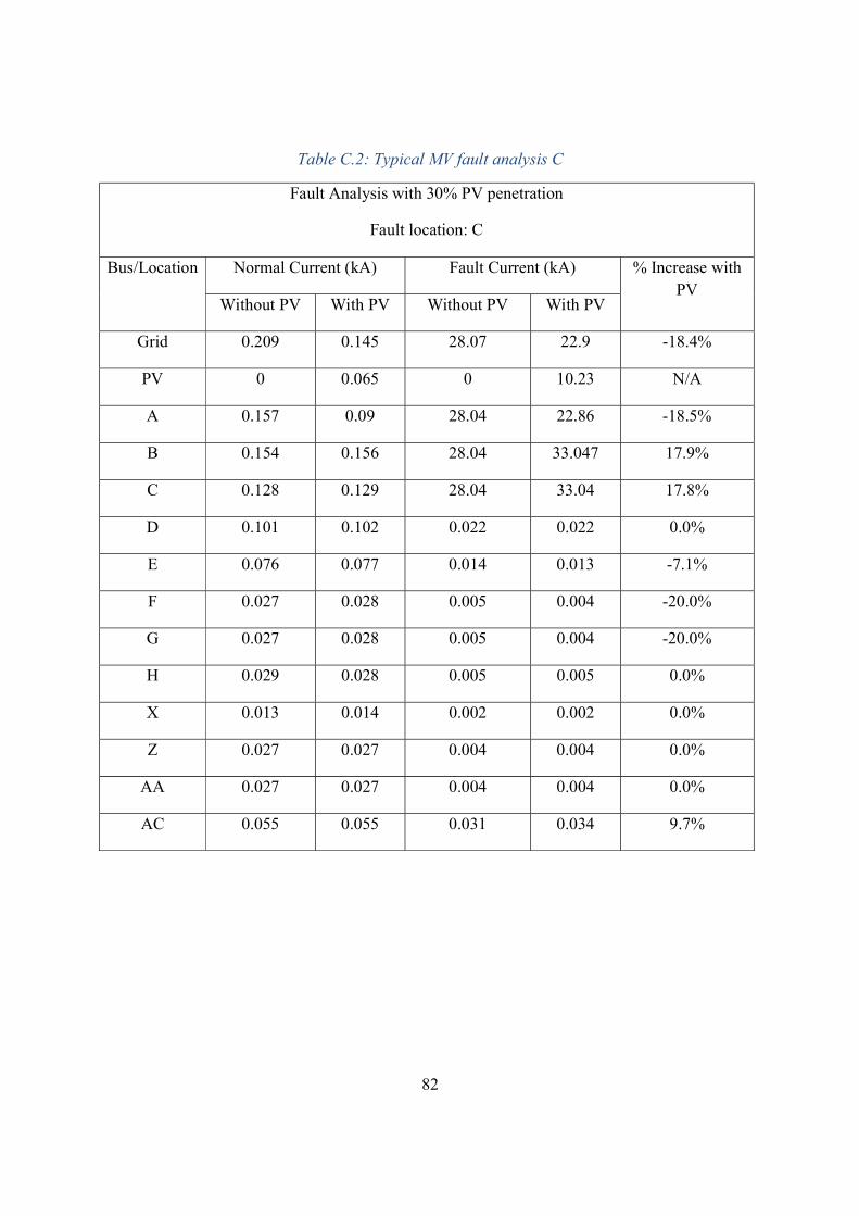
82

Table C.2: Typical MV fault analysis C Fault Analysis with 30% PV penetration

Fault location: C Bus/Location Normal Current (kA) Fault Current (kA) % Increase with

PV Without PV With PV Without PV With PV Grid 0.209 0.145 28.07 22.9 -18.4% PV 0 0.065 0 10.23 N/A A 0.157 0.09 28.04 22.86 -18.5% B 0.154 0.156 28.04 33.047 17.9% C 0.128 0.129 28.04 33.04 17.8% D 0.101 0.102 0.022 0.022 0.0% E 0.076 0.077 0.014 0.013 -7.1% F 0.027 0.028 0.005 0.004 -20.0% G 0.027 0.028 0.005 0.004 -20.0% H 0.029 0.028 0.005 0.005 0.0% X 0.013 0.014 0.002 0.002 0.0% Z 0.027 0.027 0.004 0.004 0.0%

AA 0.027 0.027 0.004 0.004 0.0% AC 0.055 0.055 0.031 0.034 9.7%

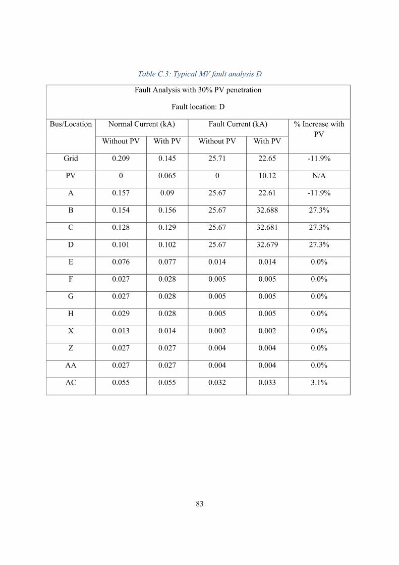
83

Table C.3: Typical MV fault analysis D Fault Analysis with 30% PV penetration

Fault location: D Bus/Location Normal Current (kA) Fault Current (kA) % Increase with

PV Without PV With PV Without PV With PV Grid 0.209 0.145 25.71 22.65 -11.9% PV 0 0.065 0 10.12 N/A A 0.157 0.09 25.67 22.61 -11.9% B 0.154 0.156 25.67 32.688 27.3% C 0.128 0.129 25.67 32.681 27.3% D 0.101 0.102 25.67 32.679 27.3% E 0.076 0.077 0.014 0.014 0.0% F 0.027 0.028 0.005 0.005 0.0% G 0.027 0.028 0.005 0.005 0.0% H 0.029 0.028 0.005 0.005 0.0% X 0.013 0.014 0.002 0.002 0.0% Z 0.027 0.027 0.004 0.004 0.0%

AA 0.027 0.027 0.004 0.004 0.0% AC 0.055 0.055 0.032 0.033 3.1%

84

Table C.4: Typical MV fault analysis E Fault Analysis with 30% PV penetration

Fault location: E Bus/Location Normal Current (kA) Fault Current (kA) % Increase with

PV Without PV With PV Without PV With PV Grid 0.209 0.145 22.5 19.169 -14.8% PV 0 0.065 0 8.562 N/A A 0.157 0.09 22.47 19.13 -14.9% B 0.154 0.156 22.47 27.659 23.1% C 0.128 0.129 22.46 27.649 23.1% D 0.101 0.102 22.45 27.644 23.1% E 0.076 0.077 22.45 27.638 23.1% F 0.027 0.028 0.005 0.005 0.0% G 0.027 0.028 0.005 0.005 0.0% H 0.029 0.028 0.005 0.005 0.0% X 0.013 0.014 0.002 0.002 0.0% Z 0.027 0.027 0.005 0.005 0.0%

AA 0.027 0.027 0.004 0.004 0.0% AC 0.055 0.055 0.036 0.039 8.3%

85

Table C.5: Typical MV analysis F Fault Analysis with 30% PV penetration

Fault location: F Bus/Location Normal Current (kA) Fault Current (kA) % Increase with

PV Without PV With PV Without PV With PV Grid 0.209 0.145 18.33 13.981 -23.7% PV 0 0.065 0 6.245 N/A A 0.157 0.09 18.29 13.938 -23.8% B 0.154 0.156 18.29 20.16 10.2% C 0.128 0.129 18.28 20.145 10.2% D 0.101 0.102 18.27 20.134 10.2% E 0.076 0.077 18.26 20.123 10.2% F 0.027 0.028 18.24 20.109 10.2% G 0.027 0.028 0.005 0.005 0.0% H 0.029 0.028 0.005 0.005 0.0% X 0.013 0.014 0.002 0.002 0.0% Z 0.027 0.027 0.008 0.008 0.0%

AA 0.027 0.027 0.007 0.008 14.3% AC 0.055 0.055 0.039 0.043 10.3%

86

Table C.6: Typical fault analysis H Fault Analysis with 30% PV penetration

Fault location: H Bus/Location Normal Current (kA) Fault Current (kA) % Increase with

PV Without PV With PV Without PV With PV Grid 0.209 0.145 10.577 6.721 -36.5% PV 0 0.065 0 5.061 N/A A 0.157 0.09 10.258 6.773 -34.0% B 0.154 0.156 10.604 11.389 7.4% C 0.128 0.129 10.594 11.379 7.4% D 0.101 0.102 10.585 11.37 7.4% E 0.076 0.077 10.526 10.723 1.9% F 0.027 0.028 9.778 10.504 7.4% G 0.027 0.028 9.778 10.504 7.4% H 0.029 0.028 9.766 10.504 7.6% X 0.013 0.014 0.003 0.002 -33.3% Z 0.027 0.027 0.02 0.021 5.0%

AA 0.027 0.027 0.021 0.02 -4.8% AC 0.055 0.055 0.0497 0.05 0.6%