Embed Size (px)
Citation preview

Master Thesis
Improvement of Speech Intelligibility for Hearing- aids
in Noisy Environment, by using the Ideal Binary Mask
Technology
Performed at the Institute for
Analysis and Scientific Computing
Of the Vienna Technical University
Under the supervision of
Ao.Univ.Prof.i.R. Dipl.-Ing. Dr.rer.nat. Dr.sc.med. Dr.techn.Frank Rattay
Co-supervisor
Univ.Lektorin Dipl.-Ing. Dr.techn.Ursula Susanne Hofstötter
By
Wars Al Karkhi, B.Sc.
Mat.Nr. 1125457
Vorgartenstrasse 87/5, 1200 Wien
July, 2017
Die approbierte Originalversion dieser Diplom-/ Masterarbeit ist in der Hauptbibliothek der Tech-nischen Universität Wien aufgestellt und zugänglich.
http://www.ub.tuwien.ac.at
The approved original version of this diploma or master thesis is available at the main library of the Vienna University of Technology.
http://www.ub.tuwien.ac.at/eng

2
Acknowledgement:
For what I achieved till now, I would deeply thank my dear family: Maalim Al Barmani, Jamal
Al Karkhy, Samer Al Karkhy, and my great supportive husband Ammar Al Mahdawi for their
great support and encouragement throughout my study and life.
I would specially thank and appreciate my Ao.Univ.Prof.Dr. Frank Rattay for giving me the
chance to work with him in this wonderful field and for his support, advices, and instructions.
Finally, I wish all who would continue working further in this field a godly blessing.

3
Improvement of the Speech Intelligibility for the Hearing-aids in noisy
environment, by using the Ideal Binary Mask Technology
Abstract:
People with hearing deficits have especially problems in speech understanding in noisy
environment (e.g. the Cocktail-party effects).
Several types of hearing-aids have shown a better signal-to-noise ratio, however, their
efficiency to improve the speech intelligibility has some limitations.
Many signal processing techniques tend to separate the speech signal from noise signal such
as many computational approaches. In spite of many researches over years, the speech
separation systems struggled to enhance the speech signal to become close to normal hearing
listeners. The ideal binary time-frequency masking is a signal separation technique that keeps
the mixture energy in the time-frequency units where local SNR (Signal-to-Noise Ratio)
exceeds a certain threshold and rejects mixture energy in other time-frequency units.
A binary mask is defined in time-frequency domain as a matrix of binary numbers, and the
elements of the speech signal in time-frequency domains are referred to as T-F units, through
this mask, the frequency band of the received signal is decomposed (simulating the human
acoustic system) by using special filters, and the energies of the signal are computed in the time
domain. The ideal binary mask IBM compares the SNR within each T-F unit with a threshold
of units of the target signal in dB, the units with SNR exceeding the threshold are signed as 1,
otherwise as 0. The IBM gain from the segregated signal can be applied again to the mixture
of target speech and noise.
Some experiments studied the effect and results of the binary masking approach for normal
hearing and hearing-impaired subjects. In this research work, we present an experiment done
by Di Lang Wang, (2009) to prove the effect of the IBM on the Speech-Reception Threshold
SRT for normal and hearing-impaired listeners, as well as, discuss the results of the experiment
and how the IBM effectively improved the speech intelligibility especially for the hearing-
impaired individuals in the cafeteria background noise. The results also proved that the speech
intelligibility has improved in the low-frequency region by the IBM more than the high-
frequency region. In the future work section we discuss the integration of the IBM technique
within the cochlear implants, which leads to elevation of the speech-recognition threshold due
to the estimation of the IBM without prior information.

4
Kurzfassung:
Menschen mit Hörproblemen haben vor allem Probleme im Sprachverständnis in lärmender
Umgebung (z. B. die Cocktailparty-Effekte).
Mehrere Arten von Hörgeräten haben ein besseres Signal-Rausch-Verhältnis gezeigt, aber ihre
Effizienz zur Verbesserung der Sprachverständlichkeit hat einige Einschränkungen.
Viele Signalverarbeitungstechniken neigen dazu, das Sprachsignal von Rauschsignal zu
trennen, wie viele Berechnungsansätze. Trotz vieler Forschungen über Jahre kämpften die
Sprachtrennsysteme, um das Sprachsignal zu verbessern, um den normalen Hörhörern nahe zu
werden. Die ideale binäre Zeit-Frequenz-Maskierung ist eine Signaltrenntechnik, die die
Gemischenergie in den Zeit-Frequenz-Einheiten hält, wo das lokale SNR (Signal-Rausch-
Verhältnis) eine bestimmte Schwelle überschreitet und die Gemischenergie in anderen Zeit-
Frequenz-Einheiten zurückweist. Eine binäre Maske wird im Zeit-Frequenz-Bereich als Matrix
von Binärzahlen definiert und die Elemente des Sprachsignals in Zeit-Frequenz-Domänen
werden als TF-Einheiten bezeichnet, durch diese Maske wird das Frequenzband des
empfangenen Signals zerlegt ( Simulation des menschlichen akustischen Systems) durch
Verwendung spezieller Filter, und die Energien des Signals werden im Zeitbereich berechnet.
Die ideale Binärmaske IBM vergleicht das SNR innerhalb jeder TF-Einheit mit einer Schwelle
von Einheiten des Zielsignals in dB, die Einheiten mit SNR, die den Schwellenwert
überschreiten, werden als 1 signiert, ansonsten als 0. Die IBM-Verstärkung aus dem
segregierten Signal kann angewendet werden Wieder auf die Mischung aus Zielsprache und
Lärm. Einige Experimente untersuchten den Effekt und die Ergebnisse des binären
Maskierungsansatzes für normale Hör- und Hörgeschädigte. In dieser Forschungsarbeit
präsentieren wir ein Experiment von Di Lang Wang (2009), um die Wirkung des IBMs auf die
Rede-Reception Threshold SRT für normale und hörbehinderte Zuhörer zu beweisen sowie die
Ergebnisse des Experiments zu diskutieren Und wie die IBM effektiv verbessert die
Sprachverständlichkeit vor allem für die Hörgeschädigten Personen in der Cafeteria
Hintergrund Lärm. Die Ergebnisse zeigten auch, dass sich die Sprachverständlichkeit im
niederfrequenten Bereich durch die IBM mehr als die Hochfrequenzregion verbessert hat. Im
künftigen Arbeitsbereich diskutieren wir die Integration der IBM-Technik innerhalb der
Cochlea-Implantate, was zu einer Erhöhung der Spracherkennungsschwelle aufgrund der
Schätzung des IBM ohne vorherige Information führt.

5
Table of content:
List of Abbreviations ................................................................................................................. 8
Chapter (1): The Anatomy of the Human Ear & Hearing
1.1 The Ear ......................................................................................................... 9
1.1.1 Introduction.................................................................... 9
1.1.2 Structure of the Auditory system ........................ 10
1.1.3 The outer ear ................................................................ 10
1.1.4 Ear drum ........................................................................ 11
1.1.5 The middle ear ............................................................ 13
1.1.6 The inner ear ................................................................ 14
1.2 Hearing ........................................................................................................ 23
1.2.1 Introduction .............................................................. 23
1.2.2 The Auditory system and transmission
of the Sound .............................................................................. 27
1.2.3 Deafness & Hearing Impairment .......................... 31
1.2.4 Severity of Hearing loss ......................................... 33
Chapter (2): Auditory Scene Analysis (ASA)
2.1 The Human Auditory Frequency Filtering ................................ 35
2.1.1 The Hearing Threshold ............................................. 35
2.1.2 The Critical band......................................................... 36
2.2 The Auditory Scene Analysis ........................................................ 39

6
2.2.1 Introduction ..................................................................... 39
2.2.2 The general Acoustic methods .............................. 42
2.2.3 The effect of perceptual arrangement of the
auditory scene analysis on the sound’s spatial
location ............................................................................ 44
2.2.4 Sound perception ........................................................ 48
2.2.5 Sequential grouping ................................................... 51
2.2.6 Simultaneous grouping ............................................. 58
Chapter (3): CASA & Ideal Binary Masking
3.1 Introduction ................................................................................................. 64
3.2 The System structure ............................................................................... 66
3.2.1 The Cochleagram ................................................................... 66
3.2.2 The Gammatone Filter ......................................................... 67
3.2.3 The signal transmission ....................................................... 68
3.2.4 Correlation of time-frequency pattern ........................... 69
3.3 The ideal binary masking ......................................................................... 70
3.3.1 Introduction ............................................................................... 70
3.3.2 The concept of Time-Frequency Masking ................... 71
3.3.3 The ideal binary mask estimation .................................... 79
3.3.4 Experiment of the Improvement of the SRT ............... 81
a) Stimuli .................................................................................................. 81
b) The process ........................................................................................ 83

7
c) Statistical analysis used ................................................................. 87
d) Results and conclusions ................................................................ 87
Chapter (4): General Conclusion & Future work
4.1 General conclusion ........................................................................................ 91
4.2 Future work ...................................................................................................... 93
References ................................................................................................................................. 94

8
List of abbreviations:
ANOVA (Analysis of variance)
ASA (Auditory scene analysis)
CASA (Computational auditory scene analysis)
CI (Cochlear implants)
dB (Decibel)
F0 (Fundamental frequency)
HI (Hearing-Impaired)
Hz (Hertz)
IBM (Ideal binary mask)
ICA (Independent component analysis)
ILD (Interaural level difference)
ITD (Interaural time difference)
LC (Local criterion)
NH (Normal hearing)
SNR (Signal-to-Noise Ratio)
SRR (Signal-to-Reverberation Ratio)
SRT (Speech recognition threshold)
SSN (Speech-Shaped noise)
STFT (Short time Fourier transform)

9
CHAPTER (1)
The Anatomy of the Human Ear and Hearing
1.1 The Ear:
1.1.1 Introduction:
The ear is the sense organ of hearing and balance in mammalians, located in a hollow space in
the temporal bone of the skull. The ear composed of three main parts: the outer, middle, and
inner ear.
Sound waves entering the ears are converted into mechanical vibrations which transmitted
through the ear drum then to the ear bones in the middle ear and reaching the cochlea in the
inner ear and then converted into nerve impulses, the nerve impulses are then transmitted to
the brain for interpretation. The ear is also responsible for the body balance and position relative
to the gravity by sending information to the brain that allows the body to maintain equilibrium.
Fig.1.1 Anatomy & Structures of the human ear
(https://www.hearinglink.org/your-hearing/balance-disorders/what-is-a-balance-disorder)

10
1.1.2 The Structure & Function of the Ear:
As mentioned previously, the ear is located in a cavity of the temporal bone. The outer ear
consists of the pinna or auricle and the auditory canal. The auditory canal is lined with glands
that secrete the wax (cerumen), the function of the wax is to trap the dust & dirt. The canal
connects the external ear to the eardrum.
The middle ear contains the ossicles, three tiny bones which are the malleus (hammer), incus
(anvil), and stapes (stirrup). The ossicles connect across the tympanic cavity to the oval window
in the cochlea. The Eustachian auditory tube connects the middle ear to the throat.
The inner ear contains the cochlea, the main organ of hearing, and the utricle, saccule, and
semicircular canals, the organs of balance and acceleration detection.
The vibrations of the ossicles travel to the cochlea, where they cause the cochlear fluid to
vibrate, and these vibrations trigger the receptors lodged in the organ of Corti, which sends
nerve impulses along the vestibulocochlear nerve (the 8th cranial nerve) to the auditory cortex
in the temporal lobe of the brain.
1.1.3 The Outer Ear:
The outer ear which is the visible part of the hearing organ, and together with eardrum they
represent the first part of sound conduction mechanism, consists of the pinna, ear canal which
lined with wax, and the outer part of the eardrum.
(Standring et. al. (2008), Richardson et. al. (2005)).
The pinna consists of the curving outer rim called the helix, the inner curved rim called the
antihelix, and opens into the ear canal. The tragus protrudes and partially obscures the ear canal,
as does the facing antitragus. The hollow region in front of the ear canal is called the concha.
The ear canal stretches for about 1 inch (2.5 cm). The first part of the canal is surrounded by
cartilage, while the second part near the eardrum is surrounded by bone. This bony part is
known as the auditory bulla and is formed by the tympanic part of the temporal bone. The skin
surrounding the ear canal contains ceruminous and sebaceous glands that produce protective
ear wax. The ear canal ends at the external surface of the eardrum.
(Drake et. al. (2005)).

11
Fig.1.2 the Structures of outer ear
(http://medical-dictionary.thefreedictionary.com/break+in+ear)
There are two types of muscles composing the outer ear: the intrinsic and extrinsic muscles,
and together with skin covering the outer ear are controlled by the facial nerve, in addition to
several nerves from the cervical plexus which supply also the external ear cavity and give
sensation to the surrounding skin.
(Moore KL, Dalley AF, Agur AM (2013). Clinically Oriented Anatomy, 7th ed. Lippincott
Williams & Wilkins. pp. 848–849)
The pinna combined an elastic cartilage, Darwin’s tubercle, and the earlobe consists of areola
and adipose tissue.
(“Plastic Surgery”, Little, Brown and Company, Boston, 1979)
1.1.4 The Eardrum:
The eardrum or tympanic membrane is a thin membrane, which separates the outer and middle
ear. The sound waves make the tympanic membrane to vibrate mechanically and the vibrations
created will travel then to the ossicles of the middle ear, and then to the oval window in the
cochlea. The main function of the eardrum, in addition to the transmission of the sound waves
from outer to the inner ear, is to amplify the sound waves in the air and send them to as
vibrations in the fluid inside the cochlea. The malleus bone closes the gap between the tympanic
membrane and other ossicles. (Purves et. al. (2012)).
12
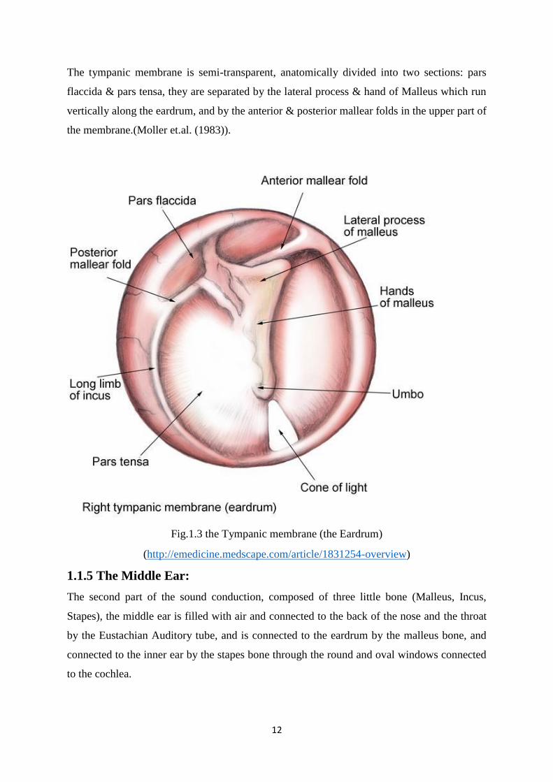
The tympanic membrane is semi-transparent, anatomically divided into two sections: pars
flaccida & pars tensa, they are separated by the lateral process & hand of Malleus which run
vertically along the eardrum, and by the anterior & posterior mallear folds in the upper part of
the membrane.(Moller et.al. (1983)).
Fig.1.3 the Tympanic membrane (the Eardrum)
(http://emedicine.medscape.com/article/1831254-overview)
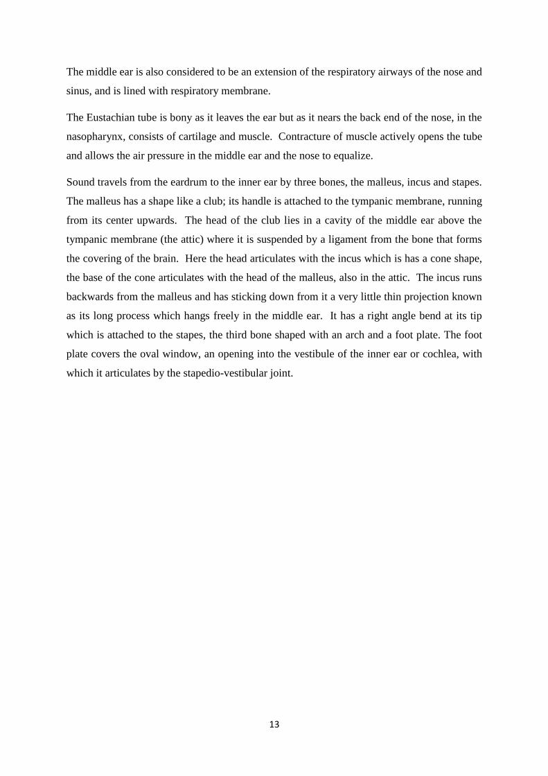
1.1.5 The Middle Ear:
The second part of the sound conduction, composed of three little bone (Malleus, Incus,
Stapes), the middle ear is filled with air and connected to the back of the nose and the throat
by the Eustachian Auditory tube, and is connected to the eardrum by the malleus bone, and
connected to the inner ear by the stapes bone through the round and oval windows connected
to the cochlea.
13
The middle ear is also considered to be an extension of the respiratory airways of the nose and
sinus, and is lined with respiratory membrane.
The Eustachian tube is bony as it leaves the ear but as it nears the back end of the nose, in the
nasopharynx, consists of cartilage and muscle. Contracture of muscle actively opens the tube
and allows the air pressure in the middle ear and the nose to equalize.
Sound travels from the eardrum to the inner ear by three bones, the malleus, incus and stapes.
The malleus has a shape like a club; its handle is attached to the tympanic membrane, running
from its center upwards. The head of the club lies in a cavity of the middle ear above the
tympanic membrane (the attic) where it is suspended by a ligament from the bone that forms
the covering of the brain. Here the head articulates with the incus which is has a cone shape,
the base of the cone articulates with the head of the malleus, also in the attic. The incus runs
backwards from the malleus and has sticking down from it a very little thin projection known
as its long process which hangs freely in the middle ear. It has a right angle bend at its tip
which is attached to the stapes, the third bone shaped with an arch and a foot plate. The foot
plate covers the oval window, an opening into the vestibule of the inner ear or cochlea, with
which it articulates by the stapedio-vestibular joint.

14
Fig.1.4 the Middle Ear
(https://www.britannica.com/science/middle-ear)
1.1.6 The Inner Ear:
It combines three areas: the semicircular canals, a central area occupied by the vestibule and
consists of two small fluid-filled cavities: the utricle & saccule, the vestibule connects the
semicircular canals with the third part that is the snail shell-like shaped cochlea with two and
a half turns. All these structures together composed the membranous labyrinth.
(Standring et.al. , (2008)).

15
The semicircular canals are structures of the bony labyrinth, each canal has a dilated end looks
like a dilated sac and called an osseous ampulla, each ampulla contains a thick gelatinous cap
called (cupula) in addition to many hair cells.
Fig.1.5 The semicircular Canals
(www.studyblue.com/anatomy&physiology)
The three canals are arranged vertically perpendicular to each other, this orientation of the
canals causes every time a stimulation to one of them, depending on the plane of the head’s
movement.
The superior and posterior canals are responsible for the equilibrium of the head when it moves
vertically up/or downward, while the horizontal one is stimulated by the angular movement or
acceleration of the head.
When the head moves, the Cupula inside the Ampulla moves in the same direction of the
movement of the head, the Cupula comprises the hair cells that are located on the top of the
Crista Ampullaris and connected to the nerve fibers, so when the hair cells are stimulated by
the movement of the Cupula, they send impulses through the nerve fibers to the brain.(Saladin
et.al. (2012)).

16
Fig.1.6 (The position of the crista ampullaris and cupula within a cross section of the ampulla
of one semicircular canal. Also shown is the movement of the cupula and its embedded cilia
during rotation first in one direction and then in the opposite direction).
(Eyzguirre et. al.(1975)).
The vestibule is the second and central partition of the inner ear, it’s located anterior to the
semicircular canals and posterior to the cochlea. It has two membranous sacs, the Utricle &
Saccule, they are also called as gravity receptors according to their responses to the gravity
forces.
On the inner surface of both Utricle & Saccule, there is a spot area of sensory cells called
(Macula), which has 2mm diameter. The Macula observes the position of the head relative to
the vertical.
In the Utricle, the macula emerges from the anterior wall of the sac in the horizontal plane,
while the macula in Saccule covers the inner wall in the vertical plane.

17
Fig.1.7 The structure of Macula: a. Vestibule, b. The Macula structures, c. the hair cell in
Macula
(http://slideplayer.com/slide/2758412/ Anatomy & physiology, Sixth Edition)
Each macula combines supporting cells, sensory hair cells, coupled with basement membrane
and nerve fibers. The hair cells are occupied from the top by the hair bundles, each bundle
comprises of about 100 nonmtile stereocilia with graded lengths & single motile Kinocilium.
When the hair bundles are deflected by a stimulation, because of a tilt of the head, the hair cells
are stimulated to alter the rate of the nerve impulses that they are constantly sending via the
vestibular nerve fibers to the brain stem.
The vestibular hair cells are of two types. Type I cells have a rounded body enclosed by a nerve
calyx; type II cells have a cylindrical body with nerve endings at the base. They form a mosaic
on the surface of the maculae, with the type I cells dominating in a curvilinear area (the Striola)
near the center of the macula and the cylindrical cells around the periphery. The significance
of these patterns is poorly understood, but they may increase sensitivity to slight tilting of the
head.

18
Fig.1.8 Type 1&2 of Hair Cells of the Macula
(https://otorrinos2do.wordpress.com/2009/12/08/physiology-of-the-vestibular-system)

19
The cochlea has a snail shell shape, comprises the membranous labyrinth and surrounded by
the fluid (perilymph).
Fig.1.9 the Cochlea (Cross-section)
(https://www.123rf.com/photo_12772769_anatomy-of-the-cochlea-of-human-ear.html)
It consists of about 30,000 hair cells, and about 19,000 nerve fibers. The hair cells receive the
sound waves in form of mechanical vibrations from the vestibular part and transform them into
nervous impulses so that they travel to & from the brain by the nerve fibers.
If we imagine the cochlea as a straight tube, it has a closed apex and opened base which has
the round & oval windows, and considered as continuity of the vestibule (which is responsible
for the head balance regarding its surroundings).
When the foot plate of the stapes vibrates, the vibrations travel to the perilymph fluid and cause
it to vibrate also, for this reason, the fluid is necessarily incompressible, and that explains the
importance of having another opening in the labyrinth to give some space to the fluid to extend

20
outward while the footplate moves inward through the oval window & inversely to move
inward when the footplate moves outward. This opening is the round window, which is located
below the oval window in the inner wall of the middle ear, and it is covered by a fibrous
membrane that moves together with the footplate of the stapes in the oval window but in the
opposite direction.
The cochlea is divided into three partitions in a triangular cross-section by a membrane which
runs along the cochlear tube. The outer two partitions are called the Scala vestibule and the
Scala tympani, they are connected to the oval and round windows respectively, and the middle
section called the cochlear duct.
Fig.1.10 The Cochlea uncoiled
(http://www1.appstate.edu/~kms/classes/psy3203/Ear/cochlea4.jpg)
21
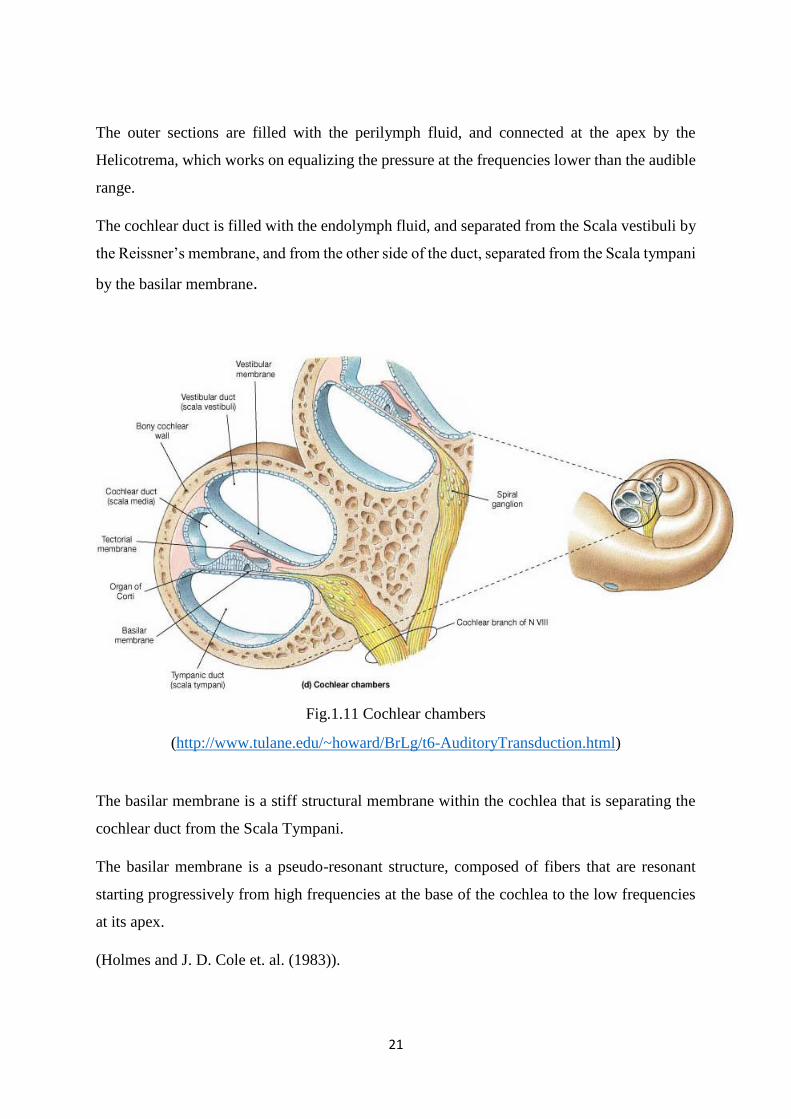
The outer sections are filled with the perilymph fluid, and connected at the apex by the
Helicotrema, which works on equalizing the pressure at the frequencies lower than the audible
range.
The cochlear duct is filled with the endolymph fluid, and separated from the Scala vestibuli by
the Reissner’s membrane, and from the other side of the duct, separated from the Scala tympani
by the basilar membrane.
Fig.1.11 Cochlear chambers
(http://www.tulane.edu/~howard/BrLg/t6-AuditoryTransduction.html)
The basilar membrane is a stiff structural membrane within the cochlea that is separating the
cochlear duct from the Scala Tympani.
The basilar membrane is a pseudo-resonant structure, composed of fibers that are resonant
starting progressively from high frequencies at the base of the cochlea to the low frequencies
at its apex.
(Holmes and J. D. Cole et. al. (1983)).

22
The basilar membrane has different properties at each point along it’s length (ex.: width,
stiffness…etc.), as it receives the sound wave, it moves generally like a travelling wave, and
each point along the membrane has different frequency characteristics according to the
stimulation caused by the sound vibrations (that is each point is sensitive to a specific frequency
matching the frequency of the incoming sound wave).
(Richard et. al. (2004)).
The width of the basilar membrane is between 0.08mm at the apex and 0.65mm at the base.
(Oghalai et. al. , (2004))
On the basilar membrane, there are four rows of the hair cells coupled by supporting cells, the
inner row of cells that is near the center of the cochlea, has an individual nerve fiber which
transmits the information to the brain, while the other 3 rows of the hair cells receive the
afferent nerve fibers from the brain.
Fig.1.12 the hair cells of Organ of Corti & the Basilar membrane
(http://slideplayer.com/slide/4213630)
Those three hair cells rows are separated from the inner row of cells by the organ of Corti.

23
As a result of any motion in any section of the cochlea, the basilar membrane experience a
motion and as a consequence a displacement of the inner hair cells would occur and send
impulses by the nerve fibers to the brain.
The hair cells have free ends called the stereocilia with few micrometers length, above the hair
cells is the tectorial membrane, the cilia of the hair cells in the outer three rows are attached to
the tectorial membrane, while the cilia of the hair cells in the inner row are free and not attached
to the membrane. These hair cells are separated & supported by Dieter’s cells that support both
the outer & inner hair cells.
The organ of Corti is the sensory organ of hearing, located in the cochlea between the Scala
Vestibuli and Scala tympani on the basilar membrane, and composed of hair cells.
The function of the organ of Corti is to transmit the auditory signals and amplify the sound
signals selected by the hair cells.
(Pujol et. al. (2013)).
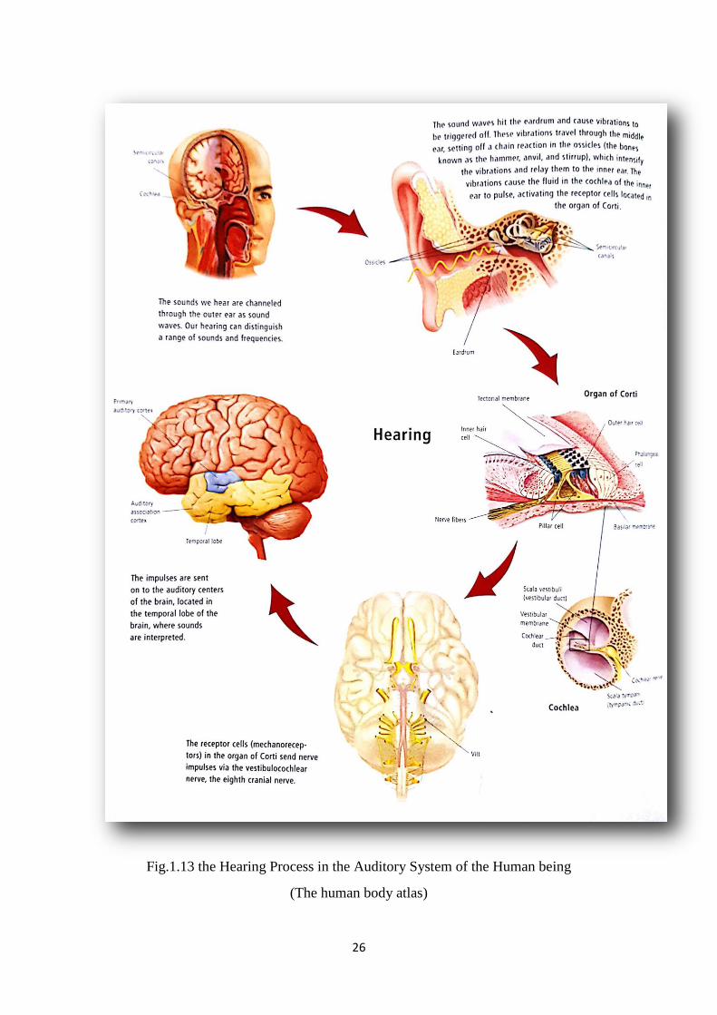
1.2 Hearing:
1.2.1 Introduction:
Hearing is the ability to receive the sound signals by detecting the sound vibrations
(Schacter et. al., (2011)).
In humans, the auditory system is responsible for the hearing process, the sound signal is first
detected by the outer ear as mechanical waves, which then transmitted to the middle ear, and
then to the inner ear, who transduce the mechanical waves to electrical impulses that are
received by the brain.
(Kung et. al. , (2005)).
The sound waves are collected by the external ear to enter the ear canal and strike the tympanic
membrane, causing the membrane to vibrate. The mechanical vibrations then transmitted to the
ossicles (the middle ear) which vibrate as a result to the transmitted sound vibrations, then
those vibrations travel to the oval window (the membrane that covers the entrance to the
cochlea), the vibrations then pass to the cochlea, where they cause the fluid inside the cochlea
to move, the movement of the fluid stimulates the hair cells which represent the mechanical
receptors in the organ of Corti.

24
The hair cells when stimulated by the mechanical movement, they send nerve impulses via the
vestibulocochlear nerve (VII cranial nerve). The impulses reach the auditory center in the
temporal region in the brain, where the sounds are processed.
(Human Body Atlas, Professor Ken Ashwell).
Sound can be consider also as a pressure wave that travels in the sound-transmitting medium
(e.g. Air), when the source of sound vibrates, a pressure wave (mechanical wave) propagates
in the transmitting medium, therefore, when the sound source vibrates, the mechanical waves
collected by the outer ear, and travel across the ear canal, reach the eardrum of the listener ear,
cause to vibrate and starting the processing of the sound.
The sound signals can be represented in two domains:
In the time-domain, the sound wave is a sequence of pressure waves with amplitudes changes
over time.
In frequency-domain, the sound wave is described as a spectrum of frequency elements that
make up the sound.
A tonal sound can be represented in time-domain as a change in amplitude (the sound pressure
values changes) of a regular sinusoidal function of the time.
As a conclusion, the sound wave can be measured in both time& frequency domains, which
means we either describe the sound as temporal fluctuations in pressure over time, or as
frequency/tonal elements that compose together the incoming sound.
The tonal sounds (as sinusoidal function) which are a frequency-domain representation, are
composed basically of complex sounds with different frequencies, such complex sounds is
called Noise.
Normally the noise is defined as a complex collection of different sounds waves with
amplitudes that changes in random way over time. There are different types of noise, e.g. the
steady-state noise SSN are white noise that comprises different frequency elements with the
almost same sound loudness or level.
Noise also can be defined as any unwanted sound that interfere with the target sound signal or
any mixture of sounds that handicap the auditory processing of the target signal in the brain.
Three crucial elements of each sound wave: Amplitude, Frequency & the duration of the wave.

25
The frequency describes how many times the sound source oscillates per second/or a period of
time, it is measured in Hertz (Hz).
Amplitude represents the magnitude of the pressure that means the amplitude of the wave is
proportional to the intensity or loudness of the heard sound, it is measured in decibel (dB), and
the decibel is the measuring unit of the sound’s level. It is the logarithm of the proportion
between two intensities or two pressures (the ratio of the intensity/Pressure at a defined period
of time to the reference intensity/Pressure), dB = 10*log 10 (I/I ref) or 20*log 10 (p/p ref).
Finally the duration of the wave is the sound duration per period of time, can be represented in
many time units, or it can be expressed as the phase of wave and measured in angular degrees.
26
Fig.1.13 the Hearing Process in the Auditory System of the Human being
(The human body atlas)

27
1.2.2 The Auditory system and transmission of the Sound:
The human ear is considered as an active energy or signal transducer, which collects & alter
the sound signal from a mechanical pressure in a sound-transmitting medium to electrical
signals via the auditory nerve to be classified and interpreted by the brain as sound, noise, or
other sound source.
Along the way from outer ear to the brain, each structure has a specific contribution the
processing of sounds’ transduction.
The outer ear consists of the Pinna, which helps to collect the sound in the surrounding
environment, the sound wave then hits the eardrum to cause it to oscillate at the same frequency
of the sound (resonance frequency) to produce mechanical pressure waves that travel across
the three bones of ossicles (the middle ear), which in turn, helps to transmit the mechanical
pressure waves into the fluid-filled inner ear.
According to the transmission of the sound wave from the air (light density medium) to a denser
medium (the fluid in inner ear), there will be some dBs loss in the sound intensity due to the
reflection of the wave at the interface between the two mediums.
The outer & middle ear serve to redirect & focus the incoming sound pressure wave towards
the inner ear, to reduce the loss of decibels as much as possible, therefore, the fluids inside the
inner ear move in an efficient manner to keep transmitting the sound signal to the brain.
Now, when the sound waves strike the tympanic membrane, it vibrates according to the
incoming sound wave, sounds of lower frequencies produce a slow rate of vibration, while
sounds of lower amplitude produce less vibration of the membrane, and the sounds of higher
frequencies lead to a faster vibration of eardrum.
The eardrum is a cone or oval shape, articulates with the ossicular chain of 3 bones of the
middle ear (malleus, incus, stapes).
The vibration of the eardrum stimulates the movement of the ossicles regarding the frequency
and amplitude of the sound pressure wave, the ossicles bones are suspended in the cavity of
ear (temporal region) and held by ligaments.
Through the movement of the ossicles, the sound pressure wave are transferred to the foot of
stapes, the stapes foot acts as a piston of action which moves inward to transmit the vibrations
into the inner ear (bony labyrinth) through the oval window.

28
The bony labyrinth is filled with a fluid called perlabyrinth [if a fluid was enclosed by
completely closed and inflexible system, then the foot of stapes couldn’t move to displace the
fluid inside the bony labyrinth, and as a result: no vibrations would be further transferred]
Because of the round window (a flexible membrane which lies underneath the oval window)
the stapes foot movement can displace the perlabyrinth allowing the vibrations to travel across
the inner ear, so the foot of stapes and the round window membrane move at the same time
(simultaneously) but in opposite directions to allow the extend of the fluid.
After the vibrations pass the oval window, the passage leads to a spiral structure of bony
labyrinth which is the cochlea. Vibrations produced by the stapes foot are drown into the spiral
system and returned to meet the round window.
The partition of the cochlea which send the sound vibrations to the apex of cochlea called the
Scala Vestibuli, the vibrations then returned through the descending partition called Scala
Tympani, and in between is the Scala Media (Cochlear duct).
The cochlear duct is filled with different fluid called the end -labyrinth, in a cross-section of
the cochlea, as we mentioned previously, two visible membranes separate the sections of
cochlea: the Riessner’s membrane (between the Scala Vetibuli and the Scala Media) and the
Basilar membrane (between the Scala Media and Scala Tympanai).
These membranes are flexible and move according to the vibrations travelling across the Scala
Vestibuli, as a result of the membranes’ movements, the vibrations are sent into the Scala
Tympani.
Fig.1.14 direction of the Vibrations
(http://www.austincc.edu/rfofi/NursingRvw/PhysText/PNSafferentpt2.html)

29
A specialized structure called the Organ of Corti is situated on the basilar membrane, as the
basilar membrane vibrates, it stimulates the organ of Corti, which sends the nerve impulses to
the brain via the vestibulocochlear nerve.
The actual nerve impulses are generated by special cells called the hair cells, and are connected
from the top to the tectorial membrane, when the basilar membrane vibrates, the stereo cilia on
the hair cells are pressed against the tectorial membrane by the movement of the basilar
membrane, pressing the stereo cilia (tiny groups of hair cells) triggering the hair cells on basilar
membrane to send nerve impulses.
Fig.1.15 the Hair cell with Stereo cilia
(http://www.austincc.edu/rfofi/NursingRvw/PhysText/PNSafferentpt2.html)

30
Fig.1.16 Organ of Corti
(http://www.austincc.edu/rfofi/NursingRvw/PhysText/PNSafferentpt2.html)
The entire basilar membrane does not oscillate simultaneously, instead, specific areas on the
membrane vibrates variably in response to different frequencies of the sound.
Fig.1.17 the tonal organization of the basilar membrane
(http://www.austincc.edu/rfofi/NursingRvw/PhysText/PNSafferentpt2.html)

31
Lower frequencies vibrates the membrane at the apex of cochlea (which is the base of the
basilar membrane), while the high frequencies vibrates the membrane near the base of cochlea
(that is the apex of basilar membrane), this arrangement is called the tonal organization (that is
the basilar membrane acts as a filter bank).
All the structures produce the auditory perception of the sounds in our surrounding
environment. (Yost et. al. , (2000)).
1.2.3 Deafness & Hearing Impairment:
Means a person is unable to hear totally or partially, the hearing loss can occur in one or both
ears, and also occur permanently or temporary. Elder people can have hearing loss with aging.
(https://www.britannica.com/science/deafness),
(http://www.who.int/mediacentre/factsheets/fs300/en/)
Causes of hearing loss can be genetically, aging, due to exposing to loud noise, or due to illness
and viral infection…etc.
The degree of hearing impairment depends on the value of the threshold, which is the minimum
decibels of sound level, at which the listener starts to hear (Human hearing starts at frequency
of 20 Hz and extends to 20 KHz with amplitude from 0 dB up to 130 dB and higher, 0 dB
represents the softest sounds while 130 dB refers to the threshold of pain).
The deafness can be defined as the degree of loss so that the listener is unable to recognize the
speech even if the speech is amplified.
(Elzouki et. al. , (2012)).
In case of total hearing loss, the person is unable to hear anything even with the presence of
loudness & amplification.
Hearing loss can occur anywhere along the auditory path, three main types of hearing loss:
conductive, sensorineural, and mixed hearing loss.
Conductive hearing impairment: refers to when the sound vibrations cannot get to the
cochlea for the nerves to transmit the signal to the brain. Different causes of conductive
loss involving excessive cerumen, wax build up, foreign bodies that enter the outer ear,
damage or tear up the tympanic membrane, excessive fluid growing in the middle ear,

32
also includes the dysfunction of the ossicular chain because of trauma that leads to
conductive hearing loss. For this kind of hearing loss, mostly treated surgically.
Sensorineural hearing loss: can be caused by loud noise damaging, aging, or other
factors, and this type of hearing impairment is present in the inner ear, resulting in
damage in the cochlea, when the hair cells are broken or de-attached, and therefore
cannot longer be triggered by the movement of the basilar membrane, and as a result,
no more of nerve impulses can reach the brain and transmit the sound information.
Normally, the hair cells which responsible for transmitting high frequencies become
damaged first since they receive the sound vibrations first. Cochlear implants are often
used as a solution for the severe degree of this type of hearing loss.
(Russell et. al. , (2013)).
Fig.1.18 Healthy VS. Damaged hair cells in sensorineural HL
(https://www.newsoundhearing.com/blog/sensorineural-hearing-loss/)
The mixed hearing loss: when the conductive & sensorineural hearing loss occur
together results from the problems in both inner & middle/ or outer ear. Treatment
may include medications, surgical solution or hearing devices (cochlear implants or
hearing aids).

33
1.2.4 Severity of Hearing loss:
Is classified according to the additional decibels of sound above the normal threshold
of hearing, and measured as the decibels of Hearing loss (dB HL), the hearing loss is
classified as:
Slight HL : 16 – 25 dB HL
Mild HL : 25 – 40 dB HL
Moderate HL : 40 – 55 dB HL
Moderate-to-Severe : 55 – 70 dB HL
Severe HL : 70 – 90 dB HL
Profound HL : 90 dB HL and more

34
Fig.1.19 Severity of HL (www.nationalhearingtest.org)
The graph (Fig.1.19) shows the degrees of the hearing loss on the left side with sound level
starts from (-10 dB) on the top, down to high sound level (120 dB) at the bottom.
On the top of the graph from left to the right, the frequency range is between 250 Hz to 8000
Hz on the right to the left respectively.

35
CHAPTER (2)
Auditory Scene Analysis (ASA)
2.1 The Human Auditory Frequency Filtering:
The audible frequency is identified as the cyclic vibration of a sound, which vibrate at a
frequency lies within the audible range of frequencies. The frequency determines the tone of
the sound.
(Pilhofer et. al. (2007)).
The standard range of audible frequencies lies between 20 Hz and 20 kHz, this range of
frequencies can alter in individuals influenced by surrounding environment. (Heffner et. al.,
(2007), (2014)).
For example, sounds with frequencies less than 20 Hz but with great enough amplitude of
sound intensity can be felt but not heard. By hearing loss (specially the sensorineural type,
when hair cells are damaged), the high sounds’ frequencies are the first not more to be heard,
because the responsible hair cells for transmitting the high frequencies are the first that receive
the sound vibration, and due to a long period of exposing to very loud Noise. (Bitner-Glindzicz,
et. al.,(2002)).
2.1.1 The Hearing Threshold:
It is the minimum level of sound of a pure tone that can a human ear receive without interfering
of other sounds. The threshold of hearing is different from one to another. (Durrant et. al.,
(1984)).
The threshold is in general mentioned as the Root Mean Square of the sound pressure of 20
micro pascal, which matches the sound intensity of 0.98 pW/m2 at 1 atmospheric pressure and
temperature of 25 C.
The lowest and quietest sound that can be detected by a healthy ear of a young individual at
the frequency of a 1000 Hz. (Gelfand et. al., (1990)).

36
The best detected sound frequencies by the human ear are between 1 kHz and 5 kHz. Since the
sound detection is frequency – related, sometimes the threshold can reach as low as -9 dB SPL.
(Jones et. al., (2014)).
Fig.2.1 The threshold oh Hearing for a healthy 20-years old showing the range of Frequencies
that can be detectable at lowest intensities dB
(http://www.psych.usyd.edu.au/staff/alexh/teaching/auditoryTute_2014/)
2.1.2 The Critical Band:
Is described as the range of audible frequencies within which a second tone will interfere with
the recognition of the first tone by the procedure of Auditory Masking. (Fletcher H. (1940)).
That means, the recognition of the sound will be reduced when a second sound with higher
intensity within the same critical band is presented, and both sounds are overlapped in time and
frequencies.

37
Fig.2.2 The Human Auditory Filters (The critical band)
(https://www.slideshare.net/franzonadiman/frequencyplacetransformation-41810312)
In the signal processing world, and in aspects of psychoacoustics, the auditory filter is a band-
pass filter that allows a specific range of frequencies to pass and hinders any frequency out of
the cut-off frequencies (as shown in the figure above).
(Gelfand et. al., (2004)).
The shape of the basilar membrane gives it the tonal organization that means the membrane
acts as a filter bank of frequencies, vibrates in resonance frequencies variably at different
points. The auditory filters presented as points associated along the basilar membrane that set
the selection of frequency in the cochlea. Due to the arrangement of frequencies on the basilar
membrane from high to low frequencies, the bandwidth decreases from the base to the apex of
the cochlear structure. (Moore et. al., (1986)), (Lyon et. al., (2010)).
The critical bandwidth in cochlea is referred to the bandwidth of the auditory filter (as
suggested by Fletcher (1940)).

38
When two sounds are vibrating simultaneously, the masking sound frequency is falling within
the critical bandwidth of auditory filter, than it participates to the masking of the other lower-
intensity sound, who it’s frequency overlaps with the masker’s frequency within the bandwidth,
and the wider is the critical band, the lower is the Signal to Noise Ratio SNR, and the more is
the sound been masked.
The equivalent rectangular bandwidth ERB is a measure in psychoacoustics that gives a
convenient approximated modeling of the human filtering bandwidth as a rectangular band-
pass filter. The ERB presents the relationship between the auditory filter, frequency and the
critical band, it is measured in Hz.
(Gelfand et. al. (2004)).
According to the Glasberg & Moore approximation of ERB for the sound of low intensities,
the ERB equation: {ERB (f) = 24.7 * (4.37 f / 1000 + 1)}, where the (f) is the center frequency
in Hz. (Moore et. al. (1998)).
Each ERB is approximately corresponds to 0.9mm on the basilar membrane, so the value of
ERB can be correspond to a specific frequency point with its position on the membrane.
For Example: when ERB = 3.36, it corresponds to a frequency point on the membrane near its
apex, while a value of ERB = 38.9 matches a frequency spot near the base of the membrane.
That means, the higher the ERB value is, the lower Frequency point which are located near the
base of the basilar membrane. (Moore et. al., (1998)).

39
2.2 The Auditory Scene Analysis
2.2.1 Introduction:
The Auditory Scene Analysis (ASA) is the process that occurs in the auditory system, by which
the incoming sound waves entering the human ear are separated into their original sources
(components that overlapped in time and frequency) and also helps to trace the path of each
sound to distinguish its sources location.
The auditory scene analysis is the basic underlying perception of the computational auditory
scene analysis (CASA).
Heuristic process are taking place in ASA to analyze the input sound signal, these processes
depends on the regularities in the incoming signal, which is a result of summation of underlying
individual sounds that make up this signal.
The heuristic processes mean the processes which enable the brain to get the sensing
information of each sound heuristically, these processes depend on the regulation and harmony
of the input signal.
For example: for an incoming signal contains different frequency elements, and these
frequencies all start at the same time, so they enter the ear as one signal, let’s say signal A,
while another set B of frequencies, which they are all received by the listener’s ear at the same
time but at different time from the A signal. Each of both A &B signals are grouped separately
depending on the regulation of the frequency components. Through the classification of the
frequency components, the pitch, timbre, loudness & spatial location of the original
components can be determined.
The first phase of sound analysis occurs in the cochlea, where the sound is resolved into
separated neural components that represent the different frequencies included in the signal
(Moore and Patterson (1986)).
For understanding the technique of separation into the original components, the scientists had
done some experiments, and their results are shown in a spectrogram, which is a picture
displays the underlying components of the sound on two axis, the X-axis represents the time,
while the Y-axis represents the frequency.

40
Fig.2.3 Spectrogram a) Mixture of Sounds b) One component of the Mixture, a spoken Word
(Bregmann: the Auditory Scene Analysis, (1990))
In the figure shown above, the dark areas at any time point and frequency refers to the intensity
of the sound at a particular time and frequency, a) refers to a received signal of the sound
mixture, the underlying individual components in this mixture could be solved if sources of the
mixture were stable, steady, have pure tone frequencies, so each horizontal line would refer to
a separated environmental source of sound regarding the period of time.
However, the figure (a) represents a mixture composed of an instrument is being played in the
background, a man who sings with different sound intensity, and another one saying the word
(Shoe).
When a listener’s ear can distinguish the word (Shoe) from the mixture, the spectrogram would
be the figure (b) showing a separated component of the mixture, and it is subtracted from the
spectrogram in (a), as we see in the mixture spectrogram, the lines that represent the
components are interact and overlap with those representing the other components or sounds,
and this the problem that facing the people with Hearing-Impairment, who are unable to
distinguish the overlapped sounds displayed at the same time.
In Bregman (1990) mentioned, that there are some processes occur in the auditory system,
serve to analyze and separate the sound mixture to its individual components, one of these

41
processes is when the auditory system store a specific sound pattern that is becoming a familiar
Schema when a similar sound signal or sound pattern enters the listener’s ear repeatedly, it will
activate the corresponding sound schema stored by the brain, and by the activation of the
schema, the ASA would give info about it for mental representation, for example, when a
person thinks he is being called by his name in surrounding environment with background
noise or randomly distributed noise like in street or in a party, also when there is a similar sound
could be heard, it can trigger the previously learned mental schema that corresponds to the
sounds pattern presenting that person’s name. This Type of recognition is automatically
happened.
Other process of recognition can take place in the auditory system for separating the sound
mixture and it’s also a learned Schema-depending process, but it happens voluntarily, for
example, when an individual tries to hear a specific voice or word, which the auditory system
has already its prior sound pattern corresponds or approximates the heard sound or word (like
a person’s name).
However, the „trying“process is an obvious signal that the voluntary listening and recognition
is included, and the process does not automatically happen.
However, in this case, the prior knowledge which is the learned schema serves as a threshold
or criterion for a particular corresponding sound or word, in trying to recognize the target sound
as long as this schema refers to the mental representation of specific characteristics.
In general, the automatic and free-willing listening requires a previously formed pattern stored
by the brain as a consequence of repeated hearing of a particular sound, so it is obvious, that it
is hard for some sounds which have no prior schema in ASA to be recognized, unless they
would be heard frequently by the listener, therefore, it is useful to have some other methods for
decomposing any incoming sound mixture into its individual elements.
It is preferred to call such methods as „ General”, or “Primal Auditory Scene Analysis”
(Bregman, 1990, p.38), primal term refers to methods depend on general auditory
characteristics used to analyse any mixture of sounds rather than using methods relay on
specific prior knowledge of specific sound or word.

42
2.2.2 The General Acoustic Methods:
Due to the problems which the Auditory Scene Analysis faces in analysing some sounds that
have no familiar corresponding pattern stored in the brain, as we mentioned in the previous
section, the usage of the general mutual acoustic characteristics, and the relations these
characteristics is very useful and necessary to solve those problems of recognizing the
incoming sound signals.
One of these general characteristics which is the harmony, that is when an object is vibrating
at a resonant frequency (standing wave pattern which is created within the vibrating object),
the small parts of this object that occupy half, quarter of the whole object, or smaller parts,
those parts will vibrate at frequencies that are twice, 4 times respectively of the primary
resonance frequency of the whole object, these frequencies are known as (the harmonic
frequencies).
An example of such objects are the strings of a musical instrument, when a person starts to play
on a guitar for example, the body of the guitar starts to vibrate till it reaches the resonance
fundamental frequency, the strings of the guitar also vibrate at frequencies, that are pure-tone
components that form the harmonic sound, those frequencies of the strings are the multiples of
the back-bone frequency of the oscillating guitar body.
At this point, we can conclude that some bodies vibrate at harmonic frequencies to produce
harmonic sounds, thus this regularity is a common characteristic of sounds in surrounding
environment, and the auditory system tries to use a strategy that utilizes this regularity to
decompose the incoming signal through its analysis of underlying pure-tone components, the
ASA can make some hypothesis about the number of sounds present in the signal to help
persuade the source of these sounds.

43
Fig.2.4 Harmonics of the Guitar Strings
(https://physics.stackexchange.com/questions/111780/why-do-harmonics-occur-when-you-
pluck-a-string)
Another probability could be made by the ASA, that a mixture signal is formed by mixing a
number of harmonic sets of sounds (let’s just say 2 sets of harmonic sounds that they
overlapped and have a share the same regularity to produce a harmonic mixture).
However, we conclude that some regularities of sounds can go into a regular relation, and at
the same time, these sounds have different sources and different time durations.
Since the harmonic frequency components that form a single mixture signal can come from the
same source and start and end at the same time, sometimes our auditory system can accept
accidentally some components or sounds that have the same harmonic components and treats
it as a part of the same sound source, while it comes from another oscillating object or source.
To avoid such a misleading, it is preferred to discover more properties and regularities that help
us to distinguish between different harmonic sounds.

44
2.2.3 The effect of perceptual arrangement of the auditory scene analysis
on the sound’s spatial location:
The regulation of sensorial proof that is performed by the ASA may influence some sides of
auditory understanding that it may not connected to the perceptual regulation interpreted by
ASA.
The arrangement can be identified as a collection of some basically pure acoustic properties
that have been originated by understanding and observance.
As an example: loudness of a received signal, this characteristics can be influenced by such
arrangements.
In Warren (1982), he described a clear example about the effect of perceptual regulation on our
understanding for localisation of the source.
This example described as (Homophonic continuity), for example, if we hear a sound with
specific constant loudness for a period of time, then suddenly the sound becomes louder for
few seconds, then returns to its previous loudness or intensity and is still continuously heard.
{Homophony: is a structure in which the backbone part is supported by one or more additional
strands that together produce the harmony and provide rhythmic contrast. Monophony in which
all parts move in unison or octaves, while polyphony in which similar lines move with rhythmic
and melodic independence to form an even structure.
(Tubb et. al., (1987), (McKay et. al., (2005)}.

45
(a)
(b)
Fig.2.5 Homophony (a) &Polyphony (b)
(http://academic.udayton.edu/PhillipMagnuson/soundpatterns/fundamentals/texture.html)
If the duration of the higher intensity sound is short, then we hear it as a second sound that has
almost the same properties of the first one except the higher intensity and identically this sound
is joined the first one, and the first sound in this case supposed it remains at fixed loudness and
continuous to be heard also behind the louder one.
The other interpretation consider that the intensity when it becomes high, it is a result of mixing
two or more lower intensity sounds, that is the loudness or intensity information of the sound
is divided between the two participating sound sources or events.

46
Fig.2.6 Two sound intensities interfering to produce one sound intensity
(https://www.quizover.com/course/section/determine-the-combined-intensity-of-two-waves-
perfect-constructive)
In other experiment, where the change in intensity does not occur suddenly, then the conception
of two sounds does not considered, but the other conception that considers the changing in
intensity of the same original sound and the high intensity heard is related to the original heard
sound.

47
Fig.2.7 Different sound intensity of the same sound source
(https://courses.lumenlearning.com/physics/chapter/17-3-sound-intensity-and-sound-level/)
In conclusion, the perceptual regulation by the ASA would determine whether the loudness
comes from one sound or from a mixture of sounds. (Bregman 1991).
To understand more about the influence of perceptual regulation on persuading the spatial
location of the sound (Bregman 1991), let’s continue with the same signal previously
mentioned, if a low intensity sound signal is introduced equally to both ears of a listener, so at
the first stage, both ears received equal amount of intensity and the sound is heard steady in the
middle, but when the sound signal that enters one of ears (let’s say the left one) suddenly
becomes louder shortly then returns to the first loudness, while the right ear is still receiving
the same first intensity of sound.
The listener’s ear is still receiving the sound in the middle, but in this time, with additional
intensity in the left, therefore, this experiment considers two sounds coming from two
locations.

48
In the same experiment, if we consider lowering the loudness of sound received by the left ear,
then the intensity of sound will be directed shortly to the left and back to the middle that means,
our spatial comprehension tends to keep tracking of any change in intensity and try to equalize
the intensity at both ears.
2.2.4 Sound Perception, Grouping & Segregation:
Many sounds are created by different sound producing sources, like sounds from surrounding
environments, noise, animals or talking persons.
Some sounds are so complex, which their spectra contain different pure tone frequency
components. As a result, those spectra would be summed and enter the listener’s ear as one
single sound.
For such a mixture, the incoming sound information have to be analyzed and separated to the
original sources, so that an accurate specific description can be formed for each individual
component.

49
Fig.2.8 Spectrogram of a speech signal contains different pure tones
(https://archive.cnx.org/contents/534e9c09-7761-47cd-97f6-f5f4a8f9193f@6/analyzing-the-
spectrum-of-speech)
The auditory streaming is a process of grouping and segregation of sensory information into
separate mental representation, also called the auditory scene analysis by Bregman (1990).
In this process, there are two types of grouping, which are the sequential and simultaneous
grouping. Sequential grouping which is a grouping the sensory information over time, while
the simultaneous grouping classify according to the frequency of the data received at the same
time. Those processes are occurring simultaneously and not independent, but we discuss them
separately.
The auditory streaming is a phenomenon in which a line contains different pitches is heard as
two or more separated tonic lines, this occurs when speech contains collection of pitches with
two or more distinguished timbres.
50
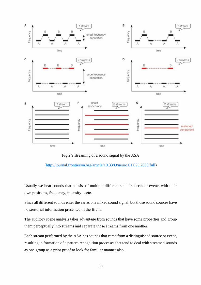
Fig.2.9 streaming of a sound signal by the ASA
(http://journal.frontiersin.org/article/10.3389/neuro.01.025.2009/full)
Usually we hear sounds that consist of multiple different sound sources or events with their
own positions, frequency, intensity….etc.
Since all different sounds enter the ear as one mixed sound signal, but those sound sources have
no sensorial information presented in the Brain.
The auditory scene analysis takes advantage from sounds that have some properties and group
them perceptually into streams and separate those streams from one another.
Each stream performed by the ASA has sounds that came from a distinguished source or event,
resulting in formation of a pattern recognition processes that tend to deal with streamed sounds
as one group as a prior proof to look for familiar manner also.

51
The frequency elements of separated sounds can overlap across the whole frequency spectrum
of a composite sound wave, and each sound wave contains multiple frequency elements.
However, those frequency components are not obliged to take a specific region of the auditory
spectrum on the basilar membrane in the Cochlea, so how can the brain classify which
components related to which sound source?
2.2.5 Sequential Grouping:
The separation of auditory streaming is necessary, and was used by Baroque composers as
(Implied Polyphony: that is one musical instrument give a sound like two).
As a simple form, when a quickly alternating melodies are heard as a trill when they have
approximated frequencies, but when they are played separately, they are separated monotonic
lines.
The trill rate used to prove the frequency separation was about 100ms tones that determines
the frequency difference about 15%, which was quite sufficient to compel a separation into two
streams.
Another experiment was done by Van Noorden to distinguish between the obliged separations
at the pretty large frequency differences and an optional separation that takes place at small
differences in frequency under attentional observation (like it’s shown in Fig.2.9).
The streaming principle based on Frequency similarities is sensitive to the difference degree
between the frequencies, the degree of segregation is proportional to the frequency difference
that is the segregation becomes stronger with larger frequency difference.
A segregated sequence of lower frequency differences is supposed to be faster than a sequence
contains higher frequency differences. (Van Noorden, 1975).
The consideration of the sequence speed can be taken as the rate of frequency changing that is
when a rapid change occurs, there is more chance that changes did not come from the same
sound source.
This property of perception process can be used to localize the sound source when a rapid
change in frequency occurs while in a series of sounds coming from the same source the
characteristics change slowly.
52
In other hand, in grouping based on frequency similarity, the auditory system tends to reduce
the change rate of frequency across time within the stream by adding more separated streams,
but in case of more complex sounds that includes a chain of harmonic frequencies of a primary
one, then the streaming couldn’t be more based on frequency, but can be settled according to
changes in timbre and to changes in pitch, also streaming can be determined by changes in
spatial position.
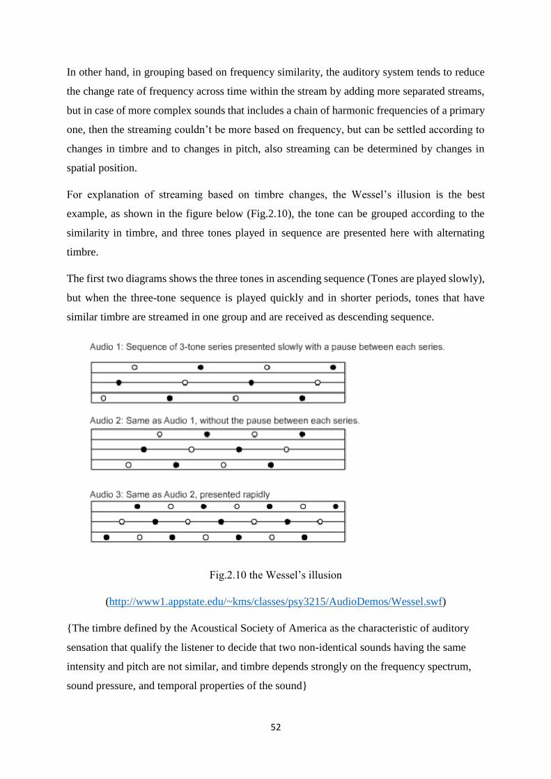
For explanation of streaming based on timbre changes, the Wessel’s illusion is the best
example, as shown in the figure below (Fig.2.10), the tone can be grouped according to the
similarity in timbre, and three tones played in sequence are presented here with alternating
timbre.
The first two diagrams shows the three tones in ascending sequence (Tones are played slowly),
but when the three-tone sequence is played quickly and in shorter periods, tones that have
similar timbre are streamed in one group and are received as descending sequence.
Fig.2.10 the Wessel’s illusion
(http://www1.appstate.edu/~kms/classes/psy3215/AudioDemos/Wessel.swf)
{The timbre defined by the Acoustical Society of America as the characteristic of auditory
sensation that qualify the listener to decide that two non-identical sounds having the same
intensity and pitch are not similar, and timbre depends strongly on the frequency spectrum,
sound pressure, and temporal properties of the sound}

53
For streaming based on changing in pitch, Darwin and Bethel Fox had performed an experiment
as shown in the figure below.
Here we have the frequencies of three formants or tones of spoken letters in resonance, and
those frequencies are alternating over time in the spectrum, when a monotonic pulse chain
triggers the resonance, it will result in a constant fundamental frequency and the listener would
hear repeated syllables (yayaya…..).
Fig.2.11 Streaming by Fundamental Frequency: A) the formant pattern is heard as the
repeating syllable (yayayaya) when played on monotone (giving a constant F0), B) is when
alternating two F0 pitches, then after a period of time, the speech starts to break up into two
different sounds like in repeating syllable (gagagaga).(Darwin: auditory grouping, 1997)
In case of exciting the resonance by alternating pulse chain between two frequencies, after a
period of repeating, the listener will hear two different sounds and each sound has different
pitch, and therefore two different pitches will be recognized.
In case of alternating resonance formants, each sound will be silent when the other one speaks,
one voice will give a formant style and silence, that is heard like (gagaga…..), while the other

54
voice performs an inquisitive sound caused by growing the first harmonic formant before
estimated ending and the first sound is phonetically improbable, and that’s because of each
sound will be heard during speaking while the other will be silent (both sounds will be heard
alternatively).
(Darwin: auditory grouping, 1997)
{A Formant defined by James Jeans, is a harmonic of a melody that is increasing by a
resonance, while the speech researcher Gunner Fant defines Formants as Spectral peaks of the
sound spectrum, but the definition that is widely used according to the Acoustical Society of
America: a formant is a range of frequencies of a complex sound, in which there is an absolute
or relative maximum in the sound spectrum, also used to mean an acoustic resonance of the
human vocal tract.
(Fant et. al., (1960)), (Titze et. al.,(1994))}.
Another streaming fundamental for sequential segregation is the spatial location, the binaural
references and evidences appear according to the situation of both ears on the sides of the head,
the sound source that is positioned far from the midline of the head results in different arrival
time of sound in both ears, and this difference in arrival time of sound to both ears determines
the difference in the path length of sound to the ears and this difference described as the
interaural time difference (ITD).
When a sound coming from one side of head (let’s say the right side), it will be heard more
intense and louder in the nearest ear (that is the right one) than in the far ear, and this results in
Interaural level difference (ILD).
55
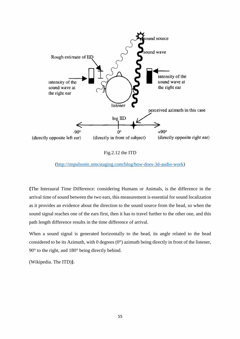
Fig.2.12 the ITD
(http://impulsonic.nmcstaging.com/blog/how-does-3d-audio-work)
{The Interaural Time Difference: considering Humans or Animals, is the difference in the
arrival time of sound between the two ears, this measurement is essential for sound localization
as it provides an evidence about the direction to the sound source from the head, so when the
sound signal reaches one of the ears first, then it has to travel further to the other one, and this
path length difference results in the time difference of arrival.
When a sound signal is generated horizontally to the head, its angle related to the head
considered to be its Azimuth, with 0 degrees (0°) azimuth being directly in front of the listener,
90° to the right, and 180° being directly behind.
(Wikipedia. The ITD)}.

56
Fig.2.13 ITD (Amplitude vs. Time in ms)
(https://en.wikipedia.org/wiki/Interaural_time_difference)
{The Interaural Intensity or Level Difference (ILD): when the sound signal heard louder in one
of the ears than in the other one, then there’s an intensity difference in the sound arrived
between the two ears, this intensity difference also helps to localize the sound source. The
intensity difference relays strongly on the frequency difference between the signals arrived to
the ears.
(Wikipedia ILD)}.

57
Fig.2.14 ILD (Wikipedia/ILD)
Fig.2.15 ILD
(http://www.hearingreview.com/2014/08/localization-101-hearing-aid-factors-localization/)
So we conclude here, that the streaming of a sound due to the spatial location could be vigorous
when a signal is continuous to be heard as a stimulus and becomes predominating at longer
time durations.
Finally, the sound properties: Timbre, Pitch, Spatial location are important cues for sequential
streaming of the sound over time. (Darwin: Auditory grouping, 1997), (Bregman, 1990).

58
2.2.6 Simultaneous Grouping:
Is the other kind of grouping that separates the sounds into streams according to the sound
sources that send the signals simultaneously, for example: many persons are talking all at the
same time.
The efficiency of simultaneous streaming deteriorates when sources generate sounds
simultaneously at harmonic frequencies that make a united melody.
When a sound is heard or played out of tune or with time delay, it becomes easier to be
recognized, also the sounds are played at non-constant time duration.
For this type of streaming, the pitch property of sound and the desynchronization are important
issues.
Pitch is a perceptual property of sounds that enables the arrangement or ordering on a
frequency-related scale (A. Klapuri et. al., (2006)) (Plack et. al., (2005)).
Let’s suppose that there are some talking persons, that in some how their speech is modified to
a monotonic pitch, which is the same pitch, it becomes harder to distinguish the target sound
than when there are different pitches.
When the pitch difference increases, it elevates the rate of receiving the words correctly from
40% to 60%, also the onset time of speech can be set as another streaming principle, since that
not all talking persons start and stop speaking at the same time.
One of the difficulties that facing the auditory scene analysis in grouping is the same
fundamental frequency because it is hard to separate their speeches, but separating could be
improved when difference in (F0) occurred and increased clearly.
The difference in pitch between simultaneous speeches helps the listener to recognize the target
speech and sound, which is one of two points help us in separation process which are
identifying the formant peaks, or grouping according to the formants of same vowels.
To demonstrate the first point, as it is shown in the figure below (Fig.2.16), the lower two
curves are related to the spectra of the two vowels /i/ as in Heed & /u/ as in Hood are performed
on a stable monotonic routine on 150 Hz that they have harmony at the same frequencies, the
vowel sound can be identified by the first peak formant frequency, and the upper curve shows
the spectra of summation of both vowels are played together.

59
When we see the curve of vowel /i/, we notice that the first formant peak frequency is nearly
disappeared and not identified, because the first peak frequency of /i/ has met with the harmonic
frequency of vowel /u/, but when the harmonic frequency of one vowel are different from the
harmonic frequency of the other, than they can be heard separately by the listener.
Fig.2.16 frequency spectra of vowel sounds
(Darwin: auditory grouping, 1997)
The Auditory system performs frequency analysis to distinguish between the united harmonics
(Fundamental frequency) and the different fundamental frequencies, those analysis take place
in the cochlea, where it has a bandwidth that is a constant proportion about 13% of fundamental
frequency.
Since some melodies are composed of complex tones with frequencies equally separated, the
harmonics that are separated by large frequency ratios are better analysed by the cochlea than
the melodies with relatively small frequency ratios.
A cochlear stimulation function can be generated from the psychophysical information from
the auditory filter (shape and bandwidth) that is approach the loudness and frequency
distribution along the basilar membrane and which corresponds the sound signal.

60
(Glasberg et. al., (1990)).
In the diagram shown in the figure below (Fig.2.17), which demonstrates the corresponding
stimulation pattern of a melody of a complex tone that includes many harmonics of the same
amplitude (that is same intensity), and distributed along the basilar membrane, (A) shows the
analysis of the first 6-9 harmonic peaks, whereby (B) shows the corresponding model of the
basilar membrane stimulation on locations occupied by the resolved harmonics (left) and
locations occupied by the unresolved harmonics (right).
Also in the same figure (Fig.2.17), it is clear in (A) that with increasing frequency, the peaks
disappeared and couldn’t be more resolved, in addition to, that the close frequencies are joining
together to generate more complicated waveform.
Fig.2.17 (A) (Normalized excitation of basilar membrane by a complicated tone)

61
Fig.2.17 (B) (the pattern of the basilar membrane movement, on the right is movement
according to resolved tones on the left, and unresolved tones on the right)
(Darwin, auditory grouping, 1997)
From the first recognized harmonics, the pitch can be determined and it corresponds to the time
model of the auditory nerve stimulation that transfer the information to the brain, but in case
of unresolved harmonics only, the brain can obtain the pitch depending on the pulses of
unresolved harmonics at the fundamental frequency only when the brain gets the information
from the generated corresponding pattern.
However, the pitch determined by the resolved harmonics is definitely better than the pitch
obtained by the generated pattern of unresolved harmonics.
(Houtsma et. al., (1990)).
In general, the males’ voices pitches are different from those obtained from females’ voices,
since the frequency range of male’s voice is less than 1kHz, and becomes complicated and
unresolved with increasing to higher frequencies, while the female’s sound frequency range is
higher in general and the analysis of harmonics becomes better at higher frequency formants.
However, to separate the male and female voices, a fundamental formant principle is a little bit
complicated but it can be considered when the differences in fundamental frequencies are
relatively large to help the listener to distinguish between the fundamental frequencies of the
sounds.
(Bird et. al., (1998)),(Culling et. al., (1993))

62
For the segregation according to location, the main evidence in sound localization is the
differences in intensity and in the phase of sound signal at both ears.
For low frequencies, the intensity cannot be taken in account for the localization issue, because
the auditory system throw out the acoustic spectra of frequencies compared in its wavelength
to its sizes and are too small to be heard, but in mixture sound signal like speech, the main issue
is the arrival time difference at the two ears in the frequency region, it is the time taken by the
sound to travel a distance from the sound source to the ear, and termed as Interaural time
difference ITD (previously defined in sequential grouping).
Unfortunately, the ITD is more effective and sufficient in the sequential streaming than the
simultaneous one, therefore, we cannot depend entirely on the ITD to segregate the
simultaneous sound signals, as an example, if we hear a number of formant-like sounds that
can compose different vowels, the vowel is influenced by which formants composed it, but not
the formants that have the same time difference ITD, also for the single resolved harmonic, we
can separate the frequency either according to the onset time or altering its tuning (that is
changing the fundamental frequencies), and for that reason, the mixture sounds cannot be
separated depending only on ITD.
(Culling et. al., (1995)).
However, the simultaneous grouping build up on ITD principle is evidential weak and striking
against the intrinsic progress in sound recognition when the listener fails to localize the target
speech coming from different directions among different and noisy speeches.
Sometimes the improving of sound recognition comes from the increasing of signal-to-noise
ratio at one ear according to acoustic shadowing from the same side of that ear, and sometimes
when sounds are detected by both ears.
(Bronkhorst et. al., (1988)).
As the ITD can help a little bit for distinguishing two different sound sources over time, an
experience is performed to test the recognition of target words in two sentences from the same
talker, and the listener has to listen to every sentence and name the possible target words that
he recognizes, the sentences differ from each other in formant frequency and their ITD.

63
The listener can recognize which target word belongs to which sentence at ITD starting from
+/- 45µs, which is corresponding to the angular separation between the two sentences of 10
degrees.
The synchronization detection takes place in the brain by synchronized detectors when the
sound enters the both ears with delay in arrival time which is the ITD, in the next figure (2.18)
where the delay line compensates for the difference in arrival time at two ears which is
presented by the sound travelling different distances to the ears, and the delay line helps to
provide information about different spatial locations from the different interaural time.
Fig.2.18 Neural circuit for detecting the ITD
(Darwin: auditory grouping, 1997)

64
CHAPTER (3)
CASA & Ideal Binary Masking
3.1 Introduction:
In our daily life scenes, a speech signal is generally distorted by noise, this effect is commonly
often called (Cocktail-party noise).
Many signal processing techniques intended to separate the speech signal from noise signal
such as many computational approaches.
In spite of many researches over years, the speech separation systems has faced many struggles
to improve the speech signal recognition and become close to normal hearing listeners
recognition.
One of those approaches is called (Computational auditory scene analysis CASA), tends to
separate speech from noise by applying means of Binary masking. (Wang & Brown, 2006)
Whereby a sound within a critical band is presented inaudible, while another louder is presented
in the same band, the louder sound tends to overcome and mask the lower intensity sound.
(Moore et. al., 2003).
According to Wang D. Lang & Brown, the CASA can be defined as the system that studies the
auditory scene analysis by means of computational methods, it imitates the human ASA in
processing, segmentation, and improving the sound source mixture in the same manner the
normal human inner ear does.
(Wang & Brown, 2006), (Wang, D. L. and Brown, G. J. (Eds.) (2006)), (Moore, B. (2003)).
In other words, the CASA systems are „ Machine listening“systems that are used to separate
the mixture of sound signals to separated streams like the human auditory system does, and
since the input signal to the human auditory system comes from one or both ears, the CASA
then receives the input signal from one or two microphones only (monaural or binaural), and
therefore, it differs from the blind signal separation technique.

65
Fig.3.1 (Block Diagram of CASA)
(http://www.sciencedirect.com)
As it is mentioned in the previous chapter and Bregman (1990), the function of ASA is
organized in two essential steps: Segmentation & Segregation.
Segmentation means separating the mixed auditory sources into streams into a neighboring
groups of time-frequency units, each group represent an individual pure tone or sound source
(Wang and Brown, 2006), and also each T-F unit represent the sound signal at a specific
Frequency and time, whereas the segregation includes putting together the T-F units, that seem
they come from the same sound source into one single flow or stream. (Bregman, 1990).
Also it’s mentioned in Chapter Two about the sequential and simultaneous segregation, each
one of them depends on different characteristics of the sound signal.
Since the T-F masking has proved a significant ability in improving the speech intelligibility
in presence of interfering noise, however, it can happen that during the estimation and
calculation of the mask the errors can occur, leading in a consequence to remove the speech
parts by the mask and storing the noise parts that result in weakness in the received output
signal and a decreased signal quality, which is evaluated by comparing the received speech
signal with the clean speech.
(Araki et al., 2005; Mowlaee et al., 2012; Wang, 2008).
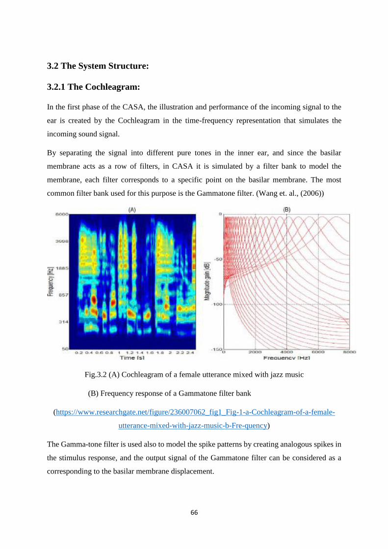
66
3.2 The System Structure:
3.2.1 The Cochleagram:
In the first phase of the CASA, the illustration and performance of the incoming signal to the
ear is created by the Cochleagram in the time-frequency representation that simulates the
incoming sound signal.
By separating the signal into different pure tones in the inner ear, and since the basilar
membrane acts as a row of filters, in CASA it is simulated by a filter bank to model the
membrane, each filter corresponds to a specific point on the basilar membrane. The most
common filter bank used for this purpose is the Gammatone filter. (Wang et. al., (2006))
Fig.3.2 (A) Cochleagram of a female utterance mixed with jazz music
(B) Frequency response of a Gammatone filter bank
(https://www.researchgate.net/figure/236007062_fig1_Fig-1-a-Cochleagram-of-a-female-
utterance-mixed-with-jazz-music-b-Fre-quency)
The Gamma-tone filter is used also to model the spike patterns by creating analogous spikes in
the stimulus response, and the output signal of the Gammatone filter can be considered as a
corresponding to the basilar membrane displacement.

67
Most of the CASA systems introduce the actin potential rate of the auditory nerve instead of
the stimulus-based one. To gain such a rate and to model the hair cells displacement, the output
signal of the filter bank are half-wave rectified then square rooted, and as a result, the rectified
half-wave corresponds the displacement which results from the movement of the hair cells
against the tectorial membrane in response to the stimulation above the threshold.
3.2.2 The Gammatone Filter:
It is a linear filter that deals with input signals that vary over the time to produce output signals
with linear behavior because the filter is composed of digital algorithms, which produce a linear
output.
Fig.3.3 Gammatone Filter
(https://www.researchgate.net/publication/221490160_Gammatone_auditory_filterbank_and_
independent_component_analysis_for_speaker_identification)
It is named as Gammatone as its response to the stimulus which is a result of Gamma
distribution and a sinusoidal tone production, therefore it is widely used to stimulate the
auditory filter bank in CASA and other artificial auditory techniques.
The output signal of a Gammatone filter is expressed by:

68
(f) represents the center frequency in Hz, (Phi in radians) refers to the phase of carrier wave,
(a) is the amplitude, (n) is the filter’s order, (b) is the bandwidth of the filter in Hz, and (t) is
the time in seconds.
So here the sinusoidal pure tone that has an amplitude is a scaled function of Gamma
distribution.
Many filters were being proposed to model the cochlear filters and hair cells according to the
shape of the model close to the cochlea, the physiological and psychological information, and
the way of application and functionality, the most used one is the Gammatone filter bank that
is more realistic and easy to apply and working. The constant bandwidth of the basilar
membrane filters is up to 1 kHz, then depending on the central frequency the bandwidth of
each filter is proportional at center frequency above 1 kHz.
Because of the different delay in output response of those filters, an additional delay is added
for compensation the differences in the time-delay of all filters and as a result, a united stimulus
response is coming out.
(Slaney, Malcolm (1993))
3.2.3 The Signal Transmission:
In the human auditory system, the stimulation of the auditory nerve depends on the mechanical
movement of the basilar membrane in response to the incoming sound’s pressure, as a result,
if the displacement of the membrane is good enough to stimulate the movement of the hair cells
against the tectorial membrane to send the sensorial signals to the auditory nerve, then the nerve
will be triggered and send the signals to the brain to be processed.
The probability of firing the auditory nerve fibers through the hair cells signals, to stimulate by
CASA, it depends on the strength and quality of the incoming signal, at this point, the
probability is positive when the properties of the transmitted signal are close to the properties
of the rectified half-wave also has pressure or compressive properties that resemble the hair
cells models characteristics, or can be modeled by non-linear algorithms.
(Meddis et. al.,(1988))
69
In some models that experience a non-linear signal transmission, it is followed up by low-pass
filtration in the time-domain, the filtration can result in showing the loss of coincidence
represented in relatively high frequencies (above 1 kHz), or it can result in ejection of repeated
feature of speech and to gain a steady voice spectrum over time and the degree of filtration
operation depends on the model used.
As a result, the output of this filtration can be shown as a series of short spectra of filtered
signals.
3.2.4 Correlation of time-frequency pattern:
The filtered transmitted output came out from the filter bank does not have the ideal properties
of a signal transmitted through the ASA and therefore, it cannot be used for the synthesis of
the time-frequency mask especially it needs frequency and temporal resolution.
In some models, the cross-correlation between the spectra of neighboring filtration channels is
proposed to support and confirm the formants representation.
In the other hand, the cross-correlogram is proposed to compensate the time difference in
arrival of acoustic signals in binaural CASA (between the right & left channels in simulation
of a human ears when they receive the sound with a slight time delay between them).
With cross-correlation, the delay in arrival time in both channels, the summation of
corresponding peaks of the sinusoidal waves can be considered as one same sound, all these
characteristics can be suitable for application of ASA principles.
With correlogram or any resembling techniques can be applied to make an extraction from the
incoming signal to result in a representation near the ideal one that is close to the pattern formed
by human ASA.
(Cooke et. al., (1991)), (Shamma et. al., (1985)).

70
For grouping and classifying the segregated T-F units into streams to be identified as the basic
target that extracted from the features of the incoming signal, we need voiced and unvoiced
segregations to generate the target pattern or mask, in this phase, the binary mask is built.
(Y Shao, S Srinivasan, Z Jin, D Wang, (2010)).
3.3 The ideal binary masking
3.3.1 Introduction:
The ideal binary time-frequency masking is a signal separation technique that keeps the mixture
energy in the time-frequency units where local SNR exceeds a certain threshold and rejects
mixture energy in other time-frequency units.
(Wang D. L., (2008))
The noise must be ejected, i.e. the sound signal quality is wrapped up und damaged and the
sound cannot be recognized.
The noise is inhibited by utilizing the binary masking, which is the time-frequency mask based
on the signal-to-reverberation ratio SRR of the individual time-frequency channels or streams.
{SRR Signal-to-Reverberation Ratio: The spatial coherence between two microphone signals
contains useful information for the statistical characterization of a sound field. The spatial
coherence can be used for instance to determine the ratio between the coherent energy and the
diffuse energy present in a room. This information, often expressed by the signal-to-reverberant
ratio (SRR)
(Naylor et. al., (2010)).
It is necessary for many applications such as speech enhancement and de-reverberation or
parametric spatial audio coding.
(Bloom et. al., (1982)), (V. Pulkki, (2007))

71
The spatial coherence has a beneficial role in estimating the SRR, only when there are two
microphones are required & placed at a near distance arbitrarily to each other, the processing
can be carried out then in the short time Fourier transform STFT}
Any T-F stream that has an SRR greater than the threshold will be stored, otherwise it will be
removed.
In experiences that took place to prove the relation between the reflection time and the speech
reception quality, the results clarified that with increased reverberation time, the speech
intelligibility is reduced.
Also the results indicated that the reverberation time would be about 0.3 to 2.0 seconds.
Additional analysis have shown that with the T-F masking, the temporary envelope that spreads
the effects of noise reflection would be also decreased.
3.3.2 The concept of Time-Frequency Masking:
As we all know, that the hearing-impaired listeners have some difficulties to understand speech
in presence of background noise (ex. Cocktail-Party effect & steady shaped noise).
{The cocktail-party effect: is the ability of an individual to focus his hearing attention on a
specific auditory stimulus, or to distinguish a speech coming out from one person standing
among persons (talking at the same time) and filter out their stimuli or conversation.
(Bronkhorst et. al., (2000))}.
Even with the modern hearing aids that amplify the sound signal and have a great ability to
reduce the background noise, however, their ability to improve the speech reception quality is
still limited. (Dillon, (2001); Moore, (2007)).
To quantify speech intelligibility in noise, we use the speech reception threshold (SRT), which
is the mixture signal-to-noise ratio required to obtain a certain intelligibility score, typically
50%.
{The speech reception threshold SRT: is the minimum intensity in decibels at which the speech
can be recognized minimally 50% of the spoken words}.

72
Hearing-impaired listeners require 3-6 dB higher Signal-to-Noise ratio SNR than normal
hearing listeners so that they achieve hearing at the same level of intensity in typical noisy
environments. (Plomp, (1994); Alcantara et. Al., (2003)).
In case of the steady noise type, ex. Speech-shaped noise (SSN), which has a spectrum
resembles the natural speech spectrum, the SRT for Hearing-Impaired people will elevate 2.5
to 7 dB (Plomp,1994), while in present of a non-steady noise or any interfering voices, the SRT
increases to higher decibels (Festen and Plomp, (1990); Hygge et. al., (1992)).
A single interfering voice or speech will demand a SRT between 10-15 dB.
(Carhart & Tillman, (1970); Festen & Plomp, (1990)).
As we can see here for a standard speech intensity, a 1dB increases in SRT will make a
reduction of 7% - 19% in the percent correct score, therefore, a rising in SRT of 2 to 3 dB will
result in preventing to understand the speech for Hearing-impaired people in a noisy
background.
(Moore, (2007)), (Wang et.al. (2009)).
The basic idea behind using the T-F masking as a technique for speech separation is not new,
for example: the wiener filter can be considered as a T-F mask shows the ratio of target energy
to the mixture energy within a T-F unit. (Louizou, (2007)).
Fig.3.4 Block diagram of a typical time–frequency (T-F) masking system for speech
separation

73
The basic idea behind using the T-F masking as a technique for speech mixture separation, for
example: the wiener filter can be considered a T-F mask for speech enhancement, the T-F mask
shows the ratio of the target energy to the mixture energy within the T-F unit.
The recent progression of the time-frequency masking system included two main sides:
T-F mask is presented in the values of 0&1, which leads to a binary T-F mask
separation.
Either the computational auditory scene analysis CASA or the independent component
analysis ICA can be used to compute the algorithms for the synthesis of the T-F mask.
(Bergman, 1990).
{The independent component analysis ICA: signal-processing world is a computational
approach that tends to separate a multi-sourced signal to its subcomponents. Two conditions
must be found: the subcomponents of the signal must be statistically independent and have a
non-Gaussian distribution. This approach is applied mostly in cocktail-party problems}.
(Stone et. al.,(2004)).
Fig.3.5 Independent Component analysis

74
(https://www.statsoft.com/Textbook/Independent-Components-Analysis)
Recent research and analysis in CASA has led to the concept of an ideal binary T-F mask as a
performance upper bound to measure how well the CASA algorithms would fulfill. (Wang &
Brown, 2006).
The elements of the mixture composing the target sound and interfering noise are presented as
a decomposition of this mixture in a two-dimensional time-frequency representation that
includes the T-F units.
An ideal binary mask is represented by a binary matrix in which the value (1) indicates that the
target energy is higher than the interfering noise energy within the T-F unit, and thus it exceeds
the pre-defined threshold, while the value (0) indicates otherwise.
The pre-defined threshold is defined as the local SNR criterion (LC) in dB units.
The ideal binary mask can be specifically expressed as:
IBM (t, f) = 1 if s (t, f) – n (t, f) > LC, OR IBM (t, f) = 0 otherwise.
The s (t, f) refers to the target energy in the unit of time & frequency, while n (t, f) refers to the
noise energy measured in dB within the same unit or element.
As long as the setting up of the binary mask demands accession to both target and noise signals
before mixing them, the binary mask matrix can be seen ideal.
A typical SNR can be gained in a binary mask if the LC=0 in the mask.
(Wang, 2005; Li and Wang, 2009).
ICA, on the other hand, it deals with the mixed sounds signals that compose the statistically
independent signals, and makes a formulation for the separation to guess the individual signal
sources in a matrix before mixing them, and this is accomplished by the machine learning
techniques.
(Hyvärinen, Karhunen, &Oja, 2001).

75
The best technique to be used for the estimation of the binary mask is CASA, since the CASA
models the cochlear performance for sound processing, i.e. when the CASA generates
responses in time-domain from the frequency analysis of the filter bank model resembles the
basilar membrane as a Cochleagram, to finally having a two-dimensional time-frequency
matrix. (Wang and Brown, 2006)
After that, the Cochleagram of the mixture is then separated into T-F units or regions, followed
by classification of the units into streams matching individual sound sources, as a results of the
classification, a binary T-F mask in two-dimensional matrix, which helps to order each
individual pure tone in the streams.
The motivation behind using the CASA for estimation of IBM is the phenomenon of the
Auditory masking that is defined by the perceptual effect which is when a higher intensity
sound dominates over the lower intensity one when both sounds are played at the same time,
and their frequencies are included within the critical band. (Moore, 2003a), so keeping noise
in T-F units with stronger target energy as done in the standard IBM definition with 0 dB LC
should not decrease the speech intelligibility. (Drullman (1995)).
As a separation technique by the ideal binary mask, when applying the mask with a local
criterion LC=0 dB to the mixture input leads to the elimination of all T-F units containing a
target energy lower than the interference energy, and thus having an intensity lower than the
LC=0, and that means, the target sound is masked by the interference sound, at the same time,
the T-F units contain target energy higher than interference energy and the target intensity
exceeds the LC=0 dB are retained, while the interference energy is removed. (Wang et. al.,
2009).
The elimination of masker sounds in the T-F units provides removing of the informational
masking which is a dominant factor for decreased speech and other modulated maskers.
(Brungart, 2001).
As a result of T-F binary mask processing, a larger improvement in speech recognition is
expected in a random noisy environment (ex. Cocktail party) than in a steady noise conditions.
(Brungart et. al., 2006)

76
As previously mentioned, the LC that is at the beginning commonly used in the T-F mask is
LC=0 dB as a standard threshold, but also altering this value will create different IBM as many
experiments indicated the relation and effect of LC on the resulted IBM. (Brungart et. al.,
2006), and those experiments had shown that the best LC values for IBM to produce perfect
speech recognition are between (0) and (-12) dB, and the speech intelligibility degree is
considered to be higher than the one presented in a speech mixture signal to the listener without
improvement, and the mostly used LC value is (-6) dB, as long as the IBM with this value
produces the highest and the perfect speech intelligibility.
In processing of speech & steady state noise SSN mixtures with the IBM, the resulted signal-
recognition-threshold SRT will be reduced about more than 7 dB for the normal hearing
persons, while the reduction for hearing impaired people exceeds 9 dB
The advantage of IBM usage for HI listeners is concentrated in the low-frequency region (up
to 1.5 kHz), while it has larger benefit for NH listeners as it improves the intelligibility in high
& low frequency ranges. (Anzalone et. al., 2006).
For applying the suitable T-F masking to segment any sound mixed signal, the binary mask is
calculated by comparing the local SNR of each unit with the LC, if the SNR is higher than the
LC, then the value (1) is set for the related T-F unit in the mask, otherwise it is (0).
Previously mentioned that the LC between 0 & -12 dB gives the best building up of the binary
mask, the LC= -6 dB is suggested as the best local intensity threshold to calculate a perfect
IBM. (Brungart et. al. (2006)).
The reason behind choosing negative local criterion values is to retain specific T-F units that
have weak target energies but greater than the noise or interference energies at the same time,
as it is indicated in the pilot test, the SRT resulted by a LC= -6 dB is higher than that resulted
by LC= 0 dB (Moore, 2003a).
Some experiments indicated that even the weak target energy, which is lower than the
interference energy, can contribute to the speech intelligibility improvement according to
Drullman’s observation. (Drullman, 1995).

77

78
Fig.3.6 Illustration of IBM
A) Cochlea gram of a target speech utterance.
B) Cochlea gram of a cafeteria background.
C) Cochlea gram of a 0 dB mixture of the speech and the background shown in A &B.
D) IBM with -6 dB LC, where 1 is indicated by white& 0 by black.
E) Cochlea gram of segregated mixture by the IBM in D.
F) IBM with 0 dB LC.
G) Cochlea gram of the segregated mixture by the IBM in (F). (Wang et al.: Speech
intelligibility with ideal binary masking, 2009).

79
As the fig.3.6 above shows the results from experiments and study the T-f mask effect with
different values of LC, as an example is taken to explain this effect on a mixture sounds signal
input of target speech and a cafeteria background noise, the SNR of the signal is 0 dB
(A) Shows the target speech, while (B) represents the background noise, and (C) is the mixture,
(D) is the IBM calculated with LC= -6 dB, and (E) displays the Cochleagram of the signal
which is masked by the IBM in (D).
As a comparison of the IBM with different LC, (F) illustrates the T-F mask with LC= 0 dB,
while (G) is the Cochleagram of the output of corresponding binary mask, we noticed that with
higher LC values, the IBM is resulted with fewer values of (1) and retains less energies from
the mixture signal.
3.3.3 The ideal binary mask estimation:
The Ideal binary mask concept is derived from the auditory masking phenomenon, which
occurs in the human inner ear (at the basilar membrane), when a weak sound signal is masked
by other sound signal with higher intensity and the frequencies of both sounds occur within the
critical band. (Moore, 2003)
This mask could be built with a previous information of target speech signals and interfering
noise, so that the value of 1 indicated by the mask shows that the target energy within a specific
T-F unit is stronger than the interfering noise energy & the value of 0 indicates otherwise.
(Wang, 2005)
Many researches had shown that the ideal binary masking can produce a strong sound
recognition
(Cooke et al, 2001, Wang, 2006).
In this section, we will suggest using CASA system to construct ideal binary mask for easy
recognition of multi-sourced sound.
The estimation of the mask using CASA will be presented in two stages, in the same manner
of the auditory scene analysis in human auditory system.
The first phase is the segmentation:

80
The input mixture (Target with interfering noise) enter the system to pass through an auditory
filter-bank in periodic time frames, then the segments are generated depending on the repeating
of the period and multi-scaled consequence analysis, i.e. onset- offset analysis, resulting in
voiced and voiceless sections segments respectively. (Hu and Wang, 2006).
In the categorization phase, the system evaluate the path of each original source in the mixture
and apply a periodic synonymy to categorize the voiced parts into simultaneous channels.
Simultaneous channel involves various segments that occurs nearly at the same time (overlap
in time), afterwards, a following categorization phase applies the speaker tone to arrange the
simultaneous channels and voiced parts over time into channels matching the speaker
vocalization.
Inside this phase: first to organize regularly the simultaneous channels or flows into the
matching voiced speech and then voiceless parts.
At the end, the CASA output would be an estimation of the ideal binary mask similar to the
basic spokesperson in the input mixture.
Such a mask is used in suspicious interpretation to get a strong speech recognition. (Srinivasan
& Wang, 2007).

81
3.3.4 Experiment of the improvement of the Speech-reception Threshold
using the IBM:
An experiment took place to evaluate the SRT with IBM for both NH & HI listeners. As a
target speech, a Dantale II Corpus was used, and as an interfering noise, a steady-shape noise
& Cafeteria background noise were utilized.
a) Stimuli:
The Dantale II Corpus was used, which contains some sentences that are registered and saved
by a Danish female speaker.
There were 15 tests lists, every list comprised ten sentences, and each sentence is spoken with
the following grammars arrangement (Name, verb, numeral, adjective, object), so that a
sentence contains 5 words, each word was chosen in a random way among other different 10
words, and as a pause between sentences, a few seconds silence separation were taken in
account, so that the listener can recognize and think about heard words.
The SSN was included within the Corpus, and was formulated by overlapping the speech words
in the corpus, while the Cafeteria interference was presented as a recorded dialogue between a
male and a female talkers in Danish, and they were setting in a Cafeteria.
To confirm the interfering of the noise with the target speech and get the temporal modification,
a long-term spectrum of SSN was included to correspond the spectrum of the corpus speech
(Johannesson, 2006), both target speech and noise were converted digitally and sampled at 20
kHz frequency.

82
Fig.3.7 Long-term Spectrum of SSN & Café Background, uttered by the root mean square
levels in one-third octave bands
(Wagener et. al., 2003; Wang et. al.,2009)
To create our Cochleagram, first of all, both the target speech and noise were handled and
processed separately from each other by a 64-channel Gammatone filter, so that we had gotten
the target and noise responses in frequency-domain within the frequency range of the filter
bank.
Then to get the time duration of those frequency-responses, they were framed into 20 ms frames
with a 50% overlap between the sequential frames, and as a consequence, we had a two-
dimensional Cochleagram of the mixture.
The SNR of the mixture was calculated during the time periods comprised speech intensity
higher than the noise intensity, and since the SSN or Cafeteria noise was presented
continuously between every two sequential sentences including the target speech, the SNR
value would be hard to compute, therefore, a silence interval of 100 ms was added before the
beginning of the next sentence for better computation of the mixture SNR. (Moore, 2003).

83
Now the IBM could be built from the resulted Cochleagram, in addition to the LC that was set
at (-6 dB), the IBM would make again the stimulus signal from the mixture.
As the IBM processing is finished, all the masking signals between the target sentences are
eliminated.
To realize the effect of the IBM processing, the mixture of the speech and background noise
was presented to the listeners also without processing or separation, and this unseparated
mixture was going through masking by the IBM that has LC in negative values, so that all the
T-F units in the rebuilding process would be included, therefore, the filtering process could be
integrated while the Cochleagram analysis was created (as it shown in Fig.3.6).
The total number of the participating listeners was 24 native Danish speakers, 12 are normal
hearing persons were in the age 25 to 50 years old, and there threshold starts at 20 dB or below
than that with frequency range of 125 Hz and 8 kHz, while the other 12 were hearing-impaired
people which were in older age between 30 to 80 years old with hearing-loss degree ranging
between mild to moderate degree and they used hearing-aids which were removed during the
experiment.
Instead of hearing aids, reparations and compensation were utilized for each HI listener
separately. All the listeners in this experiment were not informed about the objectives of the
experiment.
b) The Process:
In total of 3 lists of Dantale II were set for the experiment, each list contained 10 sentences
which were randomly chosen from the corpus test, and 4 test situations were comprised in this
experiment: two situations contained first the target sentences with the SSN and second with
the Cafeteria background noise and for both situations the IBM was used for the processing,
and another two control situations used the unseparated mixture signal. The listeners were
informed to say again as many words as they could recognize after they hear each stimulus
that matches each randomly chosen sentence, without knowing whether their repeated words
were right or wrong.
Of course the listeners were given a training in the beginning by listening to the sentences
without any interfering noise and give a feedback about what did they hear to become familiar
and recognizable for them.

84
For each listener, the total experiment consumed about 1 hour included short breaks in between.
In order to obtain the 50% SRT, the sentences were presented at SNR according to the number
of correct words informed back by the listeners in the prior phrases.
(Hanson and Ludvigsen, 2001).
During the test situation, the initial 50% SRT is determined from the first 10 phrases and the
final SRT would be an average value from the other later 20 phrases.
For the HI individuals, the initial speech intensity was 5 dB higher than the noise intensity in
the 1st experiment, and in the 2nd experiment the speech intensity is reduced to the noise
intensity level, while the NH participants, both the speech and noise were presented to them at
the same intensity level.
During the control situation for unprocessed mixed signal, the target speech intensity was
modified throughout the modification process, on the contrary of the noise intensity, which was
at a constant level.
During the T-F masking situation, when the initial SNR reduced, the IBM would be dispersed
since fewer 1’s were created to keep the effect of the binary mask, the target speech intensity
would be kept at a constant level, at the same time, the noise level would be adjusted according
to all states of the T-F mask.

85
Fig.3.8 (In 1st Experiment, the SRTs in control situations and IBM situations for the NH & HI
listeners, we notice that with negative SRT would result in better and nearly same
performance for NH & HI individuals in IBM situations)
(Wang et. al.: Speech intelligibility with ideal binary masking, 2009)

86
Fig.3.9 (In the Experiment.2 to study the effectiveness of the IBM in a range of Frequencies,
the results show that the IBM produces better SRT in low-frequency regions than in the high-
frequency ones)
(Wang et. al., 2009)
In this way, the resulted few stored T-F units had sound levels that became higher in spite of
the constant speech signal within the units, and the IBM processing occurred within a small
range of the mixture. As a result, the processed input SNR of the stimuli would be heard in all
situations even the SNR is low.
The tests took place in a sound-attenuating kiosk, where a participant was seated, and for
stimulus generation, a built-in sound card was used (Sound MAX) through a control PC (IBM
think center S50), the stimulus was presented by a head-phone (Sennheiser HD 280 Pro), but
for the HI individuals, an additional amplification was performed as a compensation for the
hearing-aids, so that the sound level of the stimuli would be higher within the comfortable
audible range, and the amplification level differs from one HI listener to another, therefore, it
has to be set for each HI individual separately before the beginning of the test.
87
c) Statistical Analysis used:
To analyse the results of experiment for studying the effects of processing and noise in all
situations, ten data sets for each situation were required.
The Analysis of variance {(ANOVA: is a collection of statistical models used to analyse the
differences among group means and their associated procedures (such as "variation" among
and between groups), in a simple definition, ANOVA provides a statistical test of whether or
not the means of several groups are equal, and therefore generalizes the t-test to more than two
groups) (Stigler (1986))}was used on the data sets from both HI & NH listeners, with the
factors of processing type (IBM & the control situation with unsegregated mixture), and with
factors of individuals type (HI & NH).
The Bonferroni test (which is a type of the post hoc test in statistics), was applied where it was
needed, to show the differences between means, whereas the Fisher least significant-difference
test was utilized as the reasonable test for a null hypothesis result. The statistics were carried
out by using „Statistica” version7.
d) Results and Conclusions:
In the Fig.3.7 shows the SRT resulted in all four test situations (for two types of noise processed
in both control condition and IBM situation), and for both NH & HI listeners.
For the NH listeners: we notice that for the unseparated mixture, with the SSN background, the
SRT mean is about -8 dB, with Cafeteria background is about -10 dB.
In case of IBM, the SRT mean (SSN-IBM) is nearly 15.50 dB, while with the (CAFÉ-IBM) is
about 20.50 dB.
The ANOVA statistics indicated that for NH individuals, the effect of the processing type and
noise type were reasonably considerable, also a considerable interaction between the
processing procedure & the noise type was noticed.
While the Bonferroni post hoc tests showed a great difference between the means.
Also we can see in the Fig.3.7 that the SRT resulted from the processing by the IBM is better
than the SRT resulted by the control condition unseparated mixture processing with neglecting
the noise type, i.e. the IBM generated lower SRT than the unseparated mixture processing.

88
In addition to the processing type, according to the type of noise, with the Café-noise, the
produced SRT is lower than the produced one with the SSN background, and the best SRT is
achieved by the IBM with the Café- background.
The lower SRT with Café-background for both processing types refers to that the NH listeners
show better speech or sound intelligibility with irregular oscillating noise than the HI ones
specially with the unseparated mixture situation.
(Festen and Plomp, 1990; Peters et. al, 1998).
Now let’s see the SRT resulted with the SSN background: the difference between the SRT
produced by the control condition for unseparated mix situation and the one produced by IBM
is about 7 dB, i.e. the produced SRT is improved using the IBM processing by 7 dB and this
corresponded to what is found by (Anzalone et. al., 2006), who used the HINT test (Nilsson et.
al., 1994), also an improvement was achieved by (Brungart et. al., 2006), who used another test
but the resulted SRT improvement was lower by 2 dB, i.e. 5 dB improvement achieved, this is
because the LC used by Brungart was 0 dB, while the LC used in this experiment was -6 dB.
This proves that the choice of LC value will influence the resulted sound threshold, and the
best choice of LC would be in negative values for best SRT.
Let’s talk about the Cafeteria background SRT, the difference between the SRT resulted by
both processing types is about 10 dB, i.e. the IBM produced lower SRT by 10 dB than the
unseparated mixture, and because of the Cafeteria noise consists of considerable transitory and
spectral modification that participates in improvement of the speech intelligibility even for the
unseparated mixture procedure better than the steady regular noise.
So from the Fig.3.7 we can say, according to the background type, the larger SRT improvement
for the NH individuals is the Café-noise for unseparated mixture situation.
Now let’s discuss the results for the HI listeners, the SRTs for the unseparated mixture
condition (control situation) are -5.50 dB, -3.70 dB for SSN and Café-background respectively,
and for the IBM processing are -15 dB, -19.50 dB for SSN and Café-background respectively.
As we said before, the statistical analysis showed that the main differences according to the
listener type, noise type and processing type were considerable, also the Bonferroni test, in
addition to the Fisher LSD post hoc test referred to a distinguishable difference in means of

89
interaction ways between the listener, noise, and processing types in control unseparated
mixture situation.
But in case of IBM, there is no considerable and remarkable difference between HI & NH
listeners, also the analysis in the Fig.3.7 showed that the IBM was more effective for the SRT
results, as long as it produces lower SRT than the unseparated mixture processing does, and
according to the noise type, the IBM is more effective with the Café-background than the SSN,
and the reason behind that is: if we compare between the recognition of speech regarding the
processing type, we see that the recognition interpretation is much effective and better, for the
unseparated mix condition, the analysis presented that the HI perform worse listening in noisy
environment. If we compare here between the HI & NH recognition performance under
unsegregated circumstances, we notice an ascending in SRT for the HI in about 2.5 dB higher
than the SRT for NH ones with SSN background, and about 6.5 dB higher than the SRT for
NH with Café-background.
In comparison with the IBM conditions, the SRT resulted by the unseparated processing would
make the speech recognition and hearing performance for HI listeners more difficult.
However, the IBM effect on the resulted SRT produced an important about 9 dB reduction in
SRT with SSN background, while with Café noise more reduction of SRT of 15 dB gain
achieved by this type of processing.
If we compare the results of IBM between the NH & HI individuals, we can see the remarkable
benefit of the IBM processing for the HI listeners, i.e. more effective for the HI ones than the
NH listeners, and the IBM processing reduced the difference in SRT between both subject
types (HI & NH), therefore, the statistical analysis found no distinguishable difference after
IBM between HI & NH listeners and specially in presence of Café noise, as a result a better
speech intelligibility can be achieved.
(Wang et. al., (2009)).
A second Experiment took place to prove the advantage of the IBM in the LF & HF regions
for both NH & HI listeners, the advantage for them was significantly higher in the LF ranges.
As stimuli, the same Dantale II phrases were used as in the first experiment, the same
background noise sources were applied: SSN & Cafe Background, as a processing condition:
IBM was utilized as in the previous experiment.

90
In case of the LF condition processing, the IBM was used to process the lower 32-frequency
channels, while the higher 32-frequency channels were processed by an all-1 mask (i.e. a mask
contains only 1 ones and no zeros), and vice versa in case of the HF range processing, where
IBM used for the higher 32-frequency channels and the all-1 mask responsible for the lower
half of the Gammatone Filter bank.
This partition of the 64-frequency channels of the Gammatone filter bank produced a frequency
separation between the HF and LF zones at nearly 1,35 KHz, while in Anzalone et. al. (2006),
the separation limit was at 1,5 KHz, the reason behind choosing 1,35 KHz was that the speech
phrases of Dantale II corpus in presentation of the Noise have more target energy allocated
more in the LF region, so that the IBM would remove more Noise-containing T-F units in the
region lower than 1 KHz.
The same listeners took part in this Experiment, and the same procedure in the previous
Experiment took place. To get different input SNR, the speech level or intensity was fixed,
while the noise level was modified.
In all-frequency condition with IBM processing, we noticed that when the SNR reduced, the
SRT decreased also to more negative values, i.e. the sound level of the stimulus is supported
by the background noise and causes a higher speech intensity (specially with the Cafe
Background), therefore, the speech level was set at a lower level than in the 1st Experiment but
comfortably audible.
From the Fig. (3.9), the results for the NH Listeners explain that in the SSN condition, the
Listeners performed better hearing in IBM processing for the LF ranges, and the all-frequency
range produced the lowest SRT value.
Also the same results was produced in case of Cafe-background, whereas the IBM processing
produced lower SRT values than with the SSN , but again, the NH listeners performed better
in the LF region than in the HF, and again the AF condition came out with the lowest SRT.
It means, that the NH have advantage of IBM in the HF zone but more advantages are
concentrated in the LF & AF ranges.
The same discussion for the results of the HI participants, as the Fig. (3.9) Illustrates, that with
the SSN & Cafe Noise processed by the IBM, also the HI Listeners get advantage of the IBM
processing in the LF ranges more than in the HF range, and the AF region resulted in the best
SRTs, also the Cafe-Noise supported the target speech phrases better than the SSN.

91
CHAPTER (4)
General Conclusion & Future work
4.1 General Conclusion:
The strong recognition of the speech in by noisy environment by the NH listeners is related to
the perceptual process done by the ASA when the listener picks out the regions in mixture
signal where the target intensity is relatively higher than the interference intensity (Miller and
Licklider, 1950; Li and Loizou, 2007).
According to behold and glimpsing, it includes separating and grouping for speech and silence
regions (Bregman, 1990).
As mentioned previously in this thesis, the people who suffering the hearing loss and perform
weak listening to the target speech in presence of the interference, that’s because their ASA
ability for segregation and grouping is very low in general, and cannot use the temporal and
spectral drops in the signal, and that’s related to the reduced frequency selectivity and
resolution. (Moore, 2007)
The T-F masking can perform as the ASA does for the HI listener, so that it improves the
selectivity and detection of the T-F regions with strong target energy, and as a result, it
improves the speech intelligibility.
Sometimes the NH listeners fail to perform a perfect speech recognition caused by misusing
the information existing in the input signal in a noisy surrounding, and this low performance
becomes worse with hearing loss or any pathology in the auditory system’s parts.
So the IBM works on equalizing the listening performance of both HI & NH listeners by doing
an ideal work of detection of the target regions.
As the results of the experiment cleared, that the best effect of the IBM for NH & HI
participants was obvious with the Café background, that’s because the Café background
included spectral and temporal dips, which contain some masking regions having information
similar to the target speech that support the target energy within these regions, and therefore,
the target energy with Café background is supposed to be higher than with the SSN
interference.

92
After the experiment, some listeners meant that the café background prevented them to
recognize the target speech by distracting the listening away from the target statements.
Lowering the SRT is inversely proportional with the informational masking that is the lowest
SRT produced by the IBM with café noise presence agree with the explanation in (Brungart et.
al., 2006), that the ideal T-F mask processing reduces predominately the informational
masking, for example, the speech statements related to one talking persons, the IBM improves
the SNR of about 20-25 dB.
In comparison of the obtained SRT in the experiment resulted with café noise, the amount of
improvement is large compared with the obtained one with SSN background, but still smaller
than that obtained in case of one speaker, and even smaller when there’s multiple competing
talkers, i.e. with multiple talkers, a large interference will prevent the HI listeners to concentrate
on the target speech, and thus a large SRT improvement will be needed. (Chang, 2004).
The results of the experiment aimed to support the researches of CASA & speech enhancement
in improving the speech intelligibility in noisy environment.
The results showed the best effect of IBM is when LC = -6 dB used for the mask construction,
and as a result, better speech recognition than with mask constructed with the common used
LC = 0 dB.
Also because with LC = -6 dB, it allows the T-F mask to store more T-F units which have
target energy is higher than the interference energy so that the SNR lies between (0 and -6 dB)
(like in Fig.3.6).
Regarding the SNR, the choice of LC = -6 dB will reduce the SNR of the out coming signal in
comparison with SNR produced with LC = 0 dB.
And now the question will be, which SNR value is the suitable one for best speech
intelligibility, i.e. best produced SRT (as an evaluation of the separation and processing
systems).
Another important conclusion from the results of Experiment.2 is that the application of speech
segregation in low frequencies is very strong and perform better than the high frequencies
region, (Fig.3.9), especially for people have hearing loss.
(Anzalone et. al., 2006).

93
On one hand, the IBM processing enhances the SRT level a great deal especially for the HI
people, more than for the NH listeners, also the results showed that the IBM processing brings
close the speech recognition levels of HI & NH listeners (regarding the interference type,
Fig.3.8).
Normally at the beginning of hearing the mixture of speech and noise, the IBM needs some
time to be estimated and constructed by the algorithms that are sophisticated for this purpose.
(Wang and Brown, 2006).
On the other hand, the amount of improvement of SRT differs according to the interference,
i.e. IBM processing produces SRT improvement reduces the blank between the HI & NH as it
is shown in the experiment results, there’s small differences in the SRT levels of both HI &
NH with both backgrounds when processed by IBM but nearly close to each other.
So the IBM processing doesn’t bring necessarily the SRT of HI & NH to the same level, and
thus a close listening performance is quite enough.
4.2 Future Work:
As the IBM technique proved its ability to enhance the speech intelligibility to listeners with
hearing loss, the next step is to develop an IBM algorithm to be integrated in the cochlear
implants, or any similar technique to the T-F masking that can improve the speech intelligibility
to the CI individuals. The struggles facing this enhancement is that in the cochlear implants,
there are no prior information used to estimate the IBM, and therefore, it should be built
evaluative depending on the information stored previously in the implants, otherwise, when an
IBM would be built without any previous information related to specific new target, in this
Case, construction of the IBM can contain errors, those errors in IBM estimation can lead to
an inverse process of selecting the T-F units, which containing noise energy greater than the
Target energy, and dropping the units containing the target energy exceeds the threshold
energy. As a coincidence, the speech-reception threshold will be elevated to a higher value that
it will getting hard for the CI recipients to recognize the target words in the presentation of
background Noise. (Kressner et. al., (2016)).
94
References:
Alcántara, J. I., Moore, B. C., Kühnel, V., & Launer, S. (2003). Evaluation of the noise
reduction system in a commercial digital hearing aid: Evaluación del sistema de reducción de
ruido en un auxiliar auditivo digital comercial. International Journal of Audiology, 42(1), 34-
42.
Anassi Klapuri, (2006). Introduction to music transcription. Signal Processing Methods for
Music Transcription, 3-20.
Anzalone, M. C., Calandruccio, L., Doherty, K. A., & Carney, L. H. (2006). Determination of
the potential benefit of time-frequency gain manipulation. Ear and hearing, 27(5), 480.
Araki, A., Kanai, T., Ishikura, T., Makita, S., Uraushihara, K., Iiyama, R., & Watanabe, M.
(2005). MyD88-deficient mice develop severe intestinal inflammation in dextran sodium
sulfate colitis. Journal of gastroenterology, 40(1), 16-23.
Bitner-Glindzicz, M. (2002). Hereditary deafness and phenotyping in humans. British medical
bulletin, 63(1), 73-94..
Bird, J., & Darwin, C. J. (1998). Effects of a difference in fundamental frequency in separating
two sentences. Psychophysical and physiological advances in hearing, 263-269..
Bregmann, A. S.: the Auditory Scene Analysis, (1990), (MIT, Cambridge, MA).
Bronkhorst, A. W., & Plomp, R. (1988). The effect of head‐induced interaural time and level
differences on speech intelligibility in noise. The Journal of the Acoustical Society of America,
83(4), 1508-1516.
Bronkhorst, A. W. (2000). The cocktail party phenomenon: A review of research on speech
intelligibility in multiple-talker conditions. Acta Acustica united with Acustica, 86(1), 117-
128.
Brungart, D. S. (2001). Informational and energetic masking effects in the perception of two
simultaneous talkers. The Journal of the Acoustical Society of America, 109(3), 1101-1109.
Brungart, D. S., Chang, P. S., Simpson, B. D., & Wang, D. (2006). Isolating the energetic
component of speech-on-speech masking with ideal time-frequency segregation. The Journal
of the Acoustical Society of America, 120(6), 4007-4018.
95
Carhart, R., Tillman, T. W.,& Olsen, W. O. (1970). Hearing aid efficiency in a competing
speech situation. J Speech Hear Res, 13, 789-811..
Chang, P. S. (2004). Exploration of behavioral, physiological, and computational approaches
to auditory scene analysis. OHIO STATE UNIV COLUMBUS DEPT OF COMPUTER AND
INFORMATION SCIENCE.
Chasin, M., & Hockley, N. S. (2014). Some characteristics of amplified music through hearing
aids. Hearing research, 308, 2-12.
Cooke, M. P. (1991). Modeling auditory processing and organization. Ph. D. Thesis, University
of Sheffield.
Culling, J. F., & Darwin, C. J. (1993). Perceptual separation of simultaneous vowels: Within
and across‐formant grouping by F 0. The Journal of the Acoustical Society of America, 93(6),
3454-3467.
Culling, J. F., & Summerfield, Q. (1995). Perceptual separation of concurrent speech sounds:
Absence of across‐frequency grouping by common interaural delay. The Journal of the
Acoustical Society of America, 98(2), 785-797.
Darwin, C. J. (1997). Auditory grouping. Trends in cognitive sciences, 1(9), 327-333.
Dillon, H. (2001). Hearing aids (Vol. 362). Sydney: Boomerang press.
Wang, D. (2005). The time dimension for scene analysis. IEEE Transactions on Neural
Networks, 16(6), 1401-1426.
Drake, Richard L.; Vogl, Wayne; Tibbitts, Adam W.M. Mitchell; illustrations by Richard;
Richardson, Paul (2005). Gray's anatomy for students. Philadelphia: Elsevier/Churchill
Livingstone. pp. 855–856.
Drullman, R. (1995). Temporal envelope and fine structure cues for speech intelligibility. The
Journal of the Acoustical Society of America, 97(1), 585-592..
Durrant, J. D., & Lovrinic, J. H. (1984). Measurements of sound. Bases of hearing science (Ed.
JP Butler). Williams and Wilkins, Baltimore, 52-84.
Elzouki, A. Y. H., Nazer, H. A., Stapleton, H. M., Oh, F. B., Whitley, W., Richard, J. &
Whitley, R. J. (2012). Textbook of Clinical Pediatrics (No. 618.92).

96
Eyzaguirre, C., & Fidone, S. J. (1975). Physiology of the nervous system: an introductory text.
Year Book Medical Pub.
Fant, G. (1960). Acoustic Theory of Speech Production. Mouton & Co, The Hague,
Netherlands.
Festen, J. M., & Plomp, R. (1990). Effects of fluctuating noise and interfering speech on the
speech‐reception threshold for impaired and normal hearing. The Journal of the Acoustical
Society of America, 88(4), 1725-1736.
Fletcher, H. (1940). Auditory patterns. Reviews of modern physics, 12(1), 47.
Gelfand, S A., 1990. Hearing: An introduction to psychological and physiological acoustics.
2nd edition. New York and Basel: Marcel Dekker.
Gelfand, S. A., & Gelfand, S. (2004). Hearing: An Introduction to Psychological and
Physiological Acoustics. CRC Press.
George Frederick McKay Music Publishing Co., (Creative Orchestration), Bainbridge Island,
WA. (Originally published by Allyn & Bacon, Boston 1963, 2nd Ed. 1965).
Glasberg, B. R., & Moore, B. C. (1990). Derivation of auditory filter shapes from notched-
noise data. Hearing research, 47(1), 103-138.
Grabb, W. C. (1979). Plastic surgery. Little Brown and Company.
Hansen, M., & Ludvigsen, C. (2001). Dantale II: Danske Hagerman sætninger [Dantale II: The
Danish Hagerman sentences]. Danish Speech Audiometry Materials (Danske
Taleaudiomaterialer), Værløse, Denmark.
Heffner, H. E., & Heffner, R. S. (2007). Hearing ranges of laboratory animals. Journal of the
American Association for Laboratory Animal Science, 46(1), 20-22.
Hygge, S., Ronnberg, J., Larsby, B., & Arlinger, S. (1992). Normal-hearing and hearing-
impaired subjects' ability to just follow conversation in competing speech, reversed speech,
and noise backgrounds. Journal of Speech, Language, and Hearing Research, 35(1), 208-215.
Holmes, M., & Cole, J. D. (1983). Pseudoresonance in the cochlea. Mechanics of Hearing.
Houtsma, A. J., & Smurzynski, J. (1990). Pitch identification and discrimination for complex
tones with many harmonics. The Journal of the Acoustical Society of America, 87(1), 304-310.

97
Hyvärinen, A., Karhunen, J., & Oja, E. (2001). Independent Component Analysis.
Johannesson R.B., 2006, output SNR measurement methods, Denmark.
Jones, P. R. (2014). What’s the quietest sound a human can hear? (Aka “Why Omega-3 fatty
acids might not cure dyslexia”).
Ken Ashwell, „ Human Body Atlas”.
Kung, C. (2005). A possible unifying principle for mechanosensation. Nature, 436(7051), 647.
Loizou, P. C. (2007). Subjective evaluation and comparison of speech enhancement
algorithms. Speech Commun, 49, 588-601.
Meddis, R. (1988). Simulation of auditory–neural transduction: Further studies. The Journal of
the Acoustical Society of America, 83(3), 1056-1063.
Miller, G. A., & Licklider, J. C. (1950). The intelligibility of interrupted speech. The Journal
of the Acoustical Society of America, 22(2), 167-173.
Moller A. (1983) Auditory Physiology. New York, NY: Academic Press;
Moore, B. C. J. (1986), "Parallels between frequency selectivity measured psychophysically
and in cochlear mechanics", Scand. Audio Suppl. (25), pp. 129–52.
Moore, B. C. J. (1998). Cochlear Hearing Loss: Physiological, Psychological and Technical
Issues.
Moore, B. (2003). An Introduction to the Psychology of Hearing (5th ed.).
Moore, B. C., & Glasberg, B. R. (2007). Modeling binaural loudness. The Journal of the
Acoustical Society of America, 121(3), 1604-1612.
Moore KL, Dalley AF, Agur AM (2013). Clinically Oriented Anatomy, Lippincott Williams
& Wilkins.848–849.
Mowlaee, P., Saeidi, R., Christensen, M. G., & Martin, R. (2012, March). Subjective and
objective quality assessment of single-channel speech separation algorithms. In Acoustics,
Speech and Signal Processing (ICASSP), 2012 IEEE International Conference on (pp. 69-
72). IEEE.

98
Nilsson, M., Soli, S. D., & Sullivan, J. A. (1994). Development of the Hearing in Noise Test
for the measurement of speech reception thresholds in quiet and in noise. The Journal of the
Acoustical Society of America, 95(2), 1085-1099.
Oghalai, J. S. (2004). The cochlear amplifier: augmentation of the traveling wave within the
inner ear. Current opinion in otolaryngology & head and neck surgery, 12(5), 431.
P. A. Naylor, E. A. P. Habets, J. Y.-C. Wen, and N. D. Gaubitch, 2010, "Models, measurement
and evaluation," in Speech De-reverberation, P. A. Naylor and N. D. Gaubitch, Eds., chapter
2, pp. 21-56.
P. J. Bloom, 1982, Evaluation of a de-reverberation technique with normal and impaired
listeners, British Journal of Audiology, pp. 167-176.
Patterson, R. D. (1986). Auditory filters and excitation patterns as representations of frequency
resolution. Frequency Selectivity in Hear-ing, 123-177.
Peters, R. W., Moore, B. C., & Baer, T. (1998). Speech reception thresholds in noise with and
without spectral and temporal dips for hearing-impaired and normally hearing people. The
Journal of the Acoustical Society of America, 103(1), 577-587.
Pilhofer, Michael (2007). Music Theory for Dummies, p.97.
Plack, Christopher J.; Andrew J. Oxenham; Richard R. Fay, eds. (2005). Pitch: Neural Coding
and Perception.
Plomp, R., Drullman, R., Festen, J. M., (1994). Effect of reducing slow temporal modulations
on speech reception. The Journal of the Acoustical Society of America, 95(5), 2670-2680.
Pujol, R., & Irving, S. (2013). The Ear.
Purves, D., Augustine, G. J., Fitzpatrick, D., Katz, L. C., LaMantia, A. S., McNamara, J. O., &
Williams, S. M. (2001). Neuroscience. Sunderland. MA: Sinauer Associates.
Lyon, R. F., Katsiamis, A. G., & Drakakis, E. M. (2010, May). History and future of auditory
filter models. In Circuits and Systems (ISCAS), Proceedings of 2010 IEEE International
Symposium on (pp. 3809-3812). IEEE.
R.R. Fay, Popper, A. N., Bacon, S. P. (2004). Compression: from cochlea to cochlear implants
(p. 228). New York: Springer.

99
Russell, J. L., Pine, H. S., & Young, D. L. (2013). Pediatric cochlear implantation. Pediatric
Clinics, 60(4), 841-863.
Saladin, Kenneth S. (2012). Anatomy and Physiology: The Unity of Form and Function. New
York: McGraw Hill. 607–8.
Schacter, Daniel L. et al., (2011), Psychology, "Worth Publishers".
Shamma, S. A. (1985). Speech processing in the auditory system I: The representation of
speech sounds in the responses of the auditory nerve. The Journal of the Acoustical Society of
America, 78(5), 1612-1621.
Slaney, M. (1993). An efficient implementation of the Patterson-Holdsworth auditory filter
bank. Apple Computer, Perception Group, Tech. Rep, 35(8).
Srinivasan, S., & Wang, D. (2007). Transforming binary uncertainties for robust speech
recognition. IEEE Transactions on Audio, Speech, and Language Processing, 15(7), 2130-
2140.
Standring, Susan (2008). Borley, Neil R., ed. Gray's Anatomy: The Anatomical Basis of
Clinical Practice, Edinburgh: Churchill Livingstone/Elsevier. Chapter 36. "External and
middle ear", p.615–631, Chapter 37. "Inner ear", 633–650.
Stone, J. V. (2004). Independent Component Analysis. A Tutorial Introduction. A Bradford
Book.
Tubb, M. (1987). Textural Constructions in Music. Journal of Music Theory, McKay, George
Frederick (2005).
Titze, I.R. (1994). Principles of Voice Production, Prentice Hall.
V. Pulkki, (2007). Spatial sound reproduction with directional audio coding. Journal of the
Audio Engineering Society, 55(6), 503-516.
Van Noorden, L. P. A. S. (1975). Temporal coherence in the perception of tone sequences.
Wang, D., & Brown, G. J. (2006). Computational auditory scene analysis: Principles,
algorithms, and applications. Wiley-IEEE press.
Wang, D. (2008). Time-frequency masking for speech separation and its potential for hearing
aid design. Trends in amplification, 12(4), 332-353.

100
Wang, D., Kjems, U., Pedersen, M. S., Boldt, J. B., & Lunner, T. (2009). Speech intelligibility
in background noise with ideal binary time-frequency masking. The Journal of the Acoustical
Society of America, 125(4), 2336-2347.
Shao, Y., Srinivasan, S., Jin, Z., & Wang, D. (2010). A computational auditory scene analysis
system for speech segregation and robust speech recognition. Computer Speech & Language,
24(1), 77-93.
Yost, W. A. (2000). Fundamentals of hearing-an introduction.