Embed Size (px)
Citation preview

Optimisation Myths and Facts as Seen in Statistical Physics
Massimo BernaschiInstitute for Applied Computing
National Research Council&
Computer Science DepartmentUniversity “La Sapienza”
Rome - [email protected]
M. Bernaschi Optimisation Myths and Facts as Seen in Statistical Physics
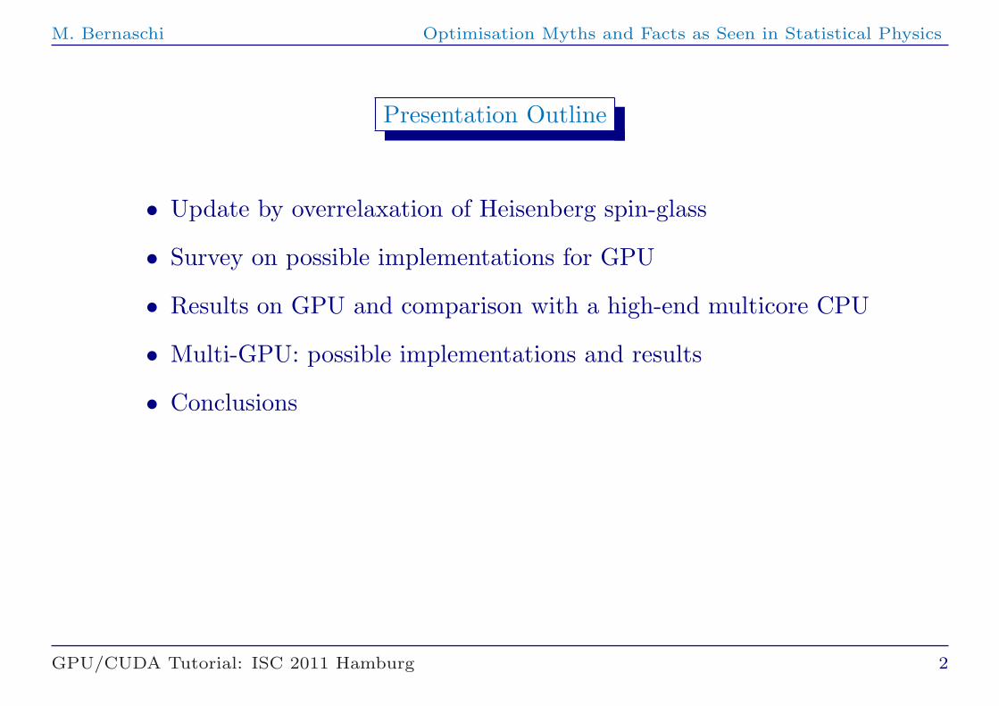
Presentation Outline
• Update by overrelaxation of Heisenberg spin-glass
• Survey on possible implementations for GPU
• Results on GPU and comparison with a high-end multicore CPU
• Multi-GPU: possible implementations and results
• Conclusions
GPU/CUDA Tutorial: ISC 2011 Hamburg 2

M. Bernaschi Optimisation Myths and Facts as Seen in Statistical Physics
The (3D) Heisenberg Spin Glass Model
A system whose energy is given by:
−�
J[x,y,z],[x±1,y±1,z±1]σ[x,y,z]σ[x±1,y±1,z±1]
where the sums run on nearest neighbors.• σ[x,y,z] is a 3-component vector [a, b, c]
– [a, b, c] ∈ R– ||σ|| =
√a2 + b2 + c2 = 1
• J[x,y,z],[x±1,y±1,z±1] ∈ R are scalar random variables withGaussian distribution:– average value equal to 0
– variance equal to 1
– for J > 0 spins tend to align but for J < 0 spins tend to misalign
spins are frustrated... and simulations take long times!
GPU/CUDA Tutorial: ISC 2011 Hamburg 3

M. Bernaschi Optimisation Myths and Facts as Seen in Statistical Physics
Update by Overrelaxation
The overrelaxation is the maximal movethat leaves the system energy invariant:foreach −→σ in (SPIN SYSTEM){
−→Hσ =
−→0
foreach n in (NEIGHBORS OF −→σ ){−→Hσ =
−→Hσ + Jn
−→σn
}−→σ = 2(
−→Hσ ·−→σ /
−→Hσ ·−→Hσ)
−→Hσ −−→σ
}
a set of scalar products that involve only simple
floating point arithmetic operations.
In 3D, for a single spin:
• 20 sums
• 3 differences
• 28 products
• one division (∼ 10 Flops).
GPU/CUDA Tutorial: ISC 2011 Hamburg 4

M. Bernaschi Optimisation Myths and Facts as Seen in Statistical Physics
Check-board decomposition
Spins can be updated in parallel if they don’t interact directly.
• Simple (check-board) decompositions of the domain can be usedto guarantee the consistency of the update procedure.
GPU/CUDA Tutorial: ISC 2011 Hamburg 5

M. Bernaschi Optimisation Myths and Facts as Seen in Statistical Physics
Data structures
Spins: each spin is a 3-component ([a, b, c]) vector.At least two alternatives (assuming C-like memory ordering).
• array of structures(good for data locality)
GPU/CUDA Tutorial: ISC 2011 Hamburg 6

M. Bernaschi Optimisation Myths and Facts as Seen in Statistical Physics
• structure of arrays(good for thread locality)
Couplings: each coupling is a scalar but there is a different couplingfor each spin in each direction (x, y, z).So we have the same possible alternatives:
Structure of Arrays (SoA) on GPU and Array of Structures(AoS) on CPU.
GPU/CUDA Tutorial: ISC 2011 Hamburg 7

M. Bernaschi Optimisation Myths and Facts as Seen in Statistical Physics
A survey of possible techniques: GPU global memory + registers (1)
A straightforward approach: each thread loads data directly fromGPU global memory to GPU registers (no shared memory variables)
• Use the structure of arraysdata layout with red andblue spins stored separately
• Two kernel invocations:one for red spins;one for blue spins.
• Very limited resource usage: 50 registers. No shared memory.
• Up to 640 threads per SM on Fermi GPUs.
GPU/CUDA Tutorial: ISC 2011 Hamburg 8

M. Bernaschi Optimisation Myths and Facts as Seen in Statistical Physics
A survey of possible techniques: GPU global memory + registers (2)
In spite of its simplicity this scheme produces a lot of data traffic:
• each spin has 6 neighbors;
• each spin loaded exactly 7 times from the Global Memory(assuming periodic boundary conditions).
• one time, by one thread, for its update;
• six times (by six other threads) to contribute to the update of itsneighbors.
It looks like a situation where GPU shared memory could come torescue...
GPU/CUDA Tutorial: ISC 2011 Hamburg 9

M. Bernaschi Optimisation Myths and Facts as Seen in Statistical Physics
A survey of possible techniques: GPU shared memory (3-plane version) (1)
An approach originally proposed to solve the Laplace equation• The domain is divided in
columns.• A single block of threads
is in charge of a column
GPU/CUDA Tutorial: ISC 2011 Hamburg 10

M. Bernaschi Optimisation Myths and Facts as Seen in Statistical Physics
A survey of possible techniques: GPU shared memory (3-plane version) (2)
Once data are in shared memory, allred spins of the active plane can beupdated concurrently then...
GPU/CUDA Tutorial: ISC 2011 Hamburg 11

M. Bernaschi Optimisation Myths and Facts as Seen in Statistical Physics
A survey of possible techniques: GPU shared memory (3-plane version) (3)
Data traffic between Global Memory and GPU processors isdramatically reduced!
• Only the spins onthe boundaries of thesubdomains need tobe loaded more thanonce.
• A spin needs to beloaded three times,at most, instead ofseven!
GPU/CUDA Tutorial: ISC 2011 Hamburg 12
M. Bernaschi Optimisation Myths and Facts as Seen in Statistical Physics
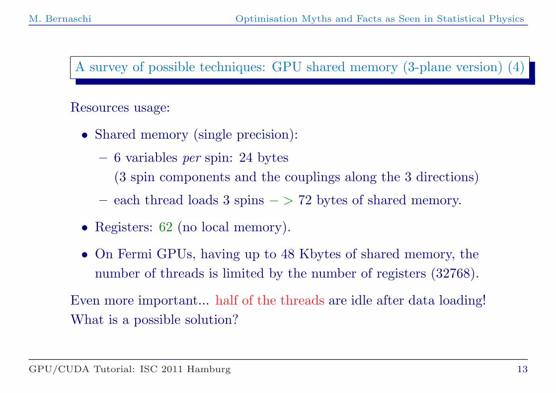
A survey of possible techniques: GPU shared memory (3-plane version) (4)
Resources usage:
• Shared memory (single precision):
– 6 variables per spin: 24 bytes(3 spin components and the couplings along the 3 directions)
– each thread loads 3 spins − > 72 bytes of shared memory.
• Registers: 62 (no local memory).
• On Fermi GPUs, having up to 48 Kbytes of shared memory, thenumber of threads is limited by the number of registers (32768).
Even more important... half of the threads are idle after data loading!What is a possible solution?
GPU/CUDA Tutorial: ISC 2011 Hamburg 13

M. Bernaschi Optimisation Myths and Facts as Seen in Statistical Physics
A survey of possible techniques: GPU shared memory (4-plane version)
Working on two planes allows to keep all threads busy!
GPU/CUDA Tutorial: ISC 2011 Hamburg 14

M. Bernaschi Optimisation Myths and Facts as Seen in Statistical Physics
In the end two planes have been updated.
• 4 planes need to be resident in shared memory.
• More shared memory per thread is required.
• Fewer threads per SM: max 384 on Fermi GPUs(the global memory version could have up to 640 threads).
Further variants are possible by replacing plain (global) memoryaccesses with texture fetches operations:
• exploit texture caching capabilities;
• make easier to manage (periodic) boundary conditions.
GPU/CUDA Tutorial: ISC 2011 Hamburg 15

M. Bernaschi Optimisation Myths and Facts as Seen in Statistical Physics
Results
Source codes and test case available from
http://www.iac.rm.cnr.it/~massimo/hsgfiles.tgz
The test case is a system having 1283 spins.
• spins and couplings are single precision variables;
• energy is accumulated in a double precision variable.
The performance measure is the time in nanoseconds required for asingle spin update (lower is better)
Tupd = TotalT ime (excluding I/O)(# of iterations)×(# of spins)
GPU/CUDA Tutorial: ISC 2011 Hamburg 16

M. Bernaschi Optimisation Myths and Facts as Seen in Statistical Physics
GM: simple Global Memory version;
ShM: Shared Memory based (3 planes);
ShM4P: Shared Memory based (4 planes);
TEXT: simple Global Memory using texture operations for data fetching.
Platform # threads Tupd
Intel X5680 (SSE instr.) 1 ∼ 13.5 ns
Intel X5680 (SSE instr. + OpenMP) 8 ∼ 3.4 ns
Tesla C1060 GM 320 1.9 ns
Tesla C1060 ShM 128 2.5 ns
Tesla C1060 ShM4P 64 2.2 ns
Tesla C1060 TEXT 320 1.8 ns
GTX 480 (Fermi) GM 320 0.66 ns
GTX 480 (Fermi) ShM 256 1.3 ns
GTX 480 (Fermi) ShM4P 192 0.86 ns
GTX 480 (Fermi) TEXT 480 0.63 ns
GPU/CUDA Tutorial: ISC 2011 Hamburg 17

M. Bernaschi Optimisation Myths and Facts as Seen in Statistical Physics
Single vs. Double precision
Platform # threads Tupd(s.p.) Tupd(d.p.)
GTX 480 (Fermi) GM 320 0.66 ns 1.3 ns
GTX 480 (Fermi) ShM4P 192/96 0.86 ns 2.2 ns
Intel X5680 3.33 Ghz (SSE instr.) 1 13.5 ns 26.6 ns
Intel X5680 3.33 Ghz (SSE instr.) 8 3.5 ns 6.8 ns
(SSE instr. + OpenMP)
GM: simple Global Memory version;
ShM4P: Shared Memory based (4 planes).
GPU/CUDA Tutorial: ISC 2011 Hamburg 18

M. Bernaschi Optimisation Myths and Facts as Seen in Statistical Physics
The Error Correcting Code effect
Platform ECC on ECC off
C2050 (Fermi) GM 1.0 ns 0.84 ns
C2050 (Fermi) ShM 1.63 ns 1.66 ns
C2050 (Fermi) ShM4P 1.4 ns 1.3 ns
C2050 (Fermi) TEXT 1.0 ns 0.78 ns
The C2050 is slightly slower than the GTX 480(14 instead of 15 SM and lower clock rate).
GPU/CUDA Tutorial: ISC 2011 Hamburg 19

M. Bernaschi Optimisation Myths and Facts as Seen in Statistical Physics
Intel X5680 “Westmere” (3.33 Ghz). Intel compiler: v. 11.1
# of cores Tupd (s.p.) no SSE Tupd (s.p.) Tupd (d.p.)
1 32.6 ns 13.6 ns 26.6 ns
2 17.8 ns 7.1 ns (96%) 15.6 ns
4 8.5 ns 4.7 ns (72%) 9.0 ns
6 6.3 ns 3.7 ns (61%) 7.4 ns
8 4.6 3.3 ns (51%) 6.8 ns
10 4.2 3.3 ns (41%) 7.0 ns
12 3.9 3.4 ns (33%) 7.0 ns
System size 1283. Very minor differences for 2563.Parallelization based on OpenMP. To “convince” the compiler thatthe innermost loop can be safely vectorized at source code level...
GPU/CUDA Tutorial: ISC 2011 Hamburg 20

REAL * __restrict__ anspx=an+spxoff,
* __restrict__ ansmx=an+smxoff;
REAL * __restrict__ anspy=an+spyoff,
* __restrict__ ansmy=an+smyoff;
REAL * __restrict__ anspz=an+spzoff,
* __restrict__ ansmz=an+smzoff;
REAL * __restrict__ bnspx=bn+spxoff,
* __restrict__ bnsmx=bn+smxoff;
REAL * __restrict__ bnspy=bn+spyoff,
* __restrict__ bnsmy=bn+smyoff;
REAL * __restrict__ bnspz=bn+spzoff,
* __restrict__ bnsmz=bn+smzoff;
REAL * __restrict__ cnspx=cn+spxoff,
* __restrict__ cnsmx=cn+smxoff;
REAL * __restrict__ cnspy=cn+spyoff,
* __restrict__ cnsmy=cn+smyoff;
REAL * __restrict__ cnspz=cn+spzoff,
* __restrict__ cnsmz=cn+smzoff;
REAL * __restrict__ JpxWO=Jpx+yzoff,
* __restrict__ JmxWO=Jmx+yzoff;
REAL * __restrict__ JpyWO=Jpy+yzoff,
* __restrict__ JmyWO=Jmy+yzoff;
REAL * __restrict__ JpzWO=Jpz+yzoff,
* __restrict__ JmzWO=Jmz+yzoff;
REAL * __restrict__ at=a+yzoff,
* __restrict__ bt=b+yzoff,
* __restrict__ ct=c+yzoff;
REAL * __restrict__ ta=t_a+yzoff,
* __restrict__ tb=t_b+yzoff,
* __restrict__ tc=t_c+yzoff;
REAL as, bs, cs, factor;
int ix;
for(ix=istart; ix<iend; ix++) {
as=anspx[ix]*JpxWO[ix]+
anspy[ix]*JpyWO[ix]+
anspz[ix]*JpzWO[ix]+
ansmx[ix]*JmxWO[ix]+
ansmy[ix]*JmyWO[ix]+
ansmz[ix]*JmzWO[ix];
bs=bnspx[ix]*JpxWO[ix]+
bnspy[ix]*JpyWO[ix]+
bnspz[ix]*JpzWO[ix]+
bnsmx[ix]*JmxWO[ix]+
bnsmy[ix]*JmyWO[ix]+
bnsmz[ix]*JmzWO[ix];
cs=cnspx[ix]*JpxWO[ix]+
cnspy[ix]*JpyWO[ix]+
cnspz[ix]*JpzWO[ix]+
cnsmx[ix]*JmxWO[ix]+
cnsmy[ix]*JmyWO[ix]+
cnsmz[ix]*JmzWO[ix]+h;
factor=two*(as*at[ix]+bs*bt[ix]+cs*ct[ix])/
(as*as+bs*bs+cs*cs);
ta[ix]=as*factor-at[ix];
tb[ix]=bs*factor-bt[ix];
tc[ix]=cs*factor-ct[ix];
}

M. Bernaschi Optimisation Myths and Facts as Seen in Statistical Physics
Multi-GPU
Simple domain decomposition along one axis
GPU/CUDA Tutorial: ISC 2011 Hamburg 22

M. Bernaschi Optimisation Myths and Facts as Seen in Statistical Physics
Multi-GPU: a first simple approach
1. compute in boundaries;
2. compute in bulk;
3. exchange data (by using CPUs!);
4. goto to 1.
GPU/CUDA Tutorial: ISC 2011 Hamburg 23

M. Bernaschi Optimisation Myths and Facts as Seen in Statistical Physics
Multi-GPU: Overlap of communication and computation
• Compute the overrelaxation for the bulkand, at the same time, exchange data forthe boundaries. Requires:– Cuda Streams
– Asynchronous Memory Copy operations
GPU/CUDA Tutorial: ISC 2011 Hamburg 24

M. Bernaschi Optimisation Myths and Facts as Seen in Statistical Physics
1. Create 2 streams: one for the boundaries, one for the bulk;
2. concurrently:
stream one starts to update the boundaries;
stream two starts to update the bulk(actually the latter starts only when the SM is available);
3. concurrently:
stream one copies data in the boundaries from the GPU to the CPU;– exchanges data among CPUs by using MPI;– copies data to the boundaries from the CPU to the GPU;
stream two continues to update the bulk;
4. go to 2.
The CPU acts as a MPI-coprocessor of the GPU!
GPU/CUDA Tutorial: ISC 2011 Hamburg 25

M. Bernaschi Optimisation Myths and Facts as Seen in Statistical Physics
Multi-GPU: Peer-to-Peer Memory Copy
• Starting on CUDA 4.0, memory copies can be performed betweentwo different GPU connected to the same PCI-e root complex.
• If peer-to-peer access is enabled then the copy operation no longerneeds to be staged through the CPU and is therefore faster!
• By using streams it remains possible to overlap communicationand computation.
GPU/CUDA Tutorial: ISC 2011 Hamburg 26

M. Bernaschi Optimisation Myths and Facts as Seen in Statistical Physics
MPI based multi-GPU results
• CPU: Dual Intel Xeon(R)X5550 @ 2.67GHz. GPU: S2050.
• QDR Infiniband connection among nodes.
• MPI intra node communication via shared memory.
# of GPU Tupd naive Tupd with Efficiency
overlap with overlap
1 0.66 ns 0.66 ns N.A.
2 0.45 ns 0.36 ns 91%
4 0.3 ns 0.19 ns 86%
8 0.22 ns 0.16 ns 51%
System size 2563. Single Precision.
GPU/CUDA Tutorial: ISC 2011 Hamburg 27

M. Bernaschi Optimisation Myths and Facts as Seen in Statistical Physics
MPI, P2P and Hybrid multi-GPU results
• 8 2050 GPU with the same Hw configuration;
• Reference time from the 2563 test case
– 5123 does not fit in a single GPU.
MPI P2P Speedup Efficiency
8 1 5.02 63%
4 2 5.91 74%
2 4 6.80 85%
1 8 7.70 96%
System size 5123. Single Precision.
GPU/CUDA Tutorial: ISC 2011 Hamburg 28

M. Bernaschi Optimisation Myths and Facts as Seen in Statistical Physics
Efficiency with up to 32 (2070) GPU for a 5123 system.
GPU/CUDA Tutorial: ISC 2011 Hamburg 29

M. Bernaschi Optimisation Myths and Facts as Seen in Statistical Physics
Conclusions
Disclaimer: What follows applies to the Heisenberg spin glass modeland very likely to other spins systems.Any inference for other computational problems is at your own risk!
• GPU implementations outperform any CPU implementation.
• Vector instructions are absolutely required to get higherperformances on multi-core CPUs.
• High end multi-core CPUs may show poor scalability.
• Multi-GPU programming is no more complex than hybridOpenMP/vector programming but...
– both Peer-to-Peer copy and MPI explicit message passingmust be overlapped with GPU kernels execution.
GPU/CUDA Tutorial: ISC 2011 Hamburg 30

M. Bernaschi Optimisation Myths and Facts as Seen in Statistical Physics
Thanks!
GPU/CUDA Tutorial: ISC 2011 Hamburg 31