Martingales in Banach Spaces (in connection with Type and Cotype

Martingales in Banach Spaces

(in connection with Type and Cotype)

Course IHP

Feb 2-8, 2011

Gilles Pisier

February 9, 2011

2

Contents

Introduction 1

1 Banach space valued martingales 111.1 B-valued Lp-spaces. Conditional expectations . . . . . . . . . . . 111.2 Martingales: basic properties . . . . . . . . . . . . . . . . . . . . 151.3 Examples of filtrations . . . . . . . . . . . . . . . . . . . . . . . . 171.4 Almost sure convergence. Maximal inequalities . . . . . . . . . . 201.5 Reverse martingales . . . . . . . . . . . . . . . . . . . . . . . . . 301.6 Notes and Remarks . . . . . . . . . . . . . . . . . . . . . . . . . . 31

2 Radon Nikodym property 332.1 Martingales, dentability and the RNP . . . . . . . . . . . . . . . 332.2 The Krein Milman property . . . . . . . . . . . . . . . . . . . . 462.3 Edgar’s Choquet Theorem . . . . . . . . . . . . . . . . . . . . . 482.4 Notes and Remarks . . . . . . . . . . . . . . . . . . . . . . . . . . 48

3 Super-reflexivity 513.1 Finite representability and Super-properties . . . . . . . . . . . 513.2 Super-reflexivity and basic sequences . . . . . . . . . . . . . . . . 553.3 Uniformly non-square and J-convex spaces . . . . . . . . . . . . 683.4 Super-reflexivity and uniform convexity . . . . . . . . . . . . . . 753.5 Notes and Remarks . . . . . . . . . . . . . . . . . . . . . . . . . . 81Appendix 1: Ultrafilters. Ultraproducts . . . . . . . . . . . . . . . . . 82

4 Uniformly convex valued martingales 854.1 Uniform convexity . . . . . . . . . . . . . . . . . . . . . . . . . . 854.2 Uniform smoothness . . . . . . . . . . . . . . . . . . . . . . . . . 984.3 Uniform convexity and smoothness of Lp . . . . . . . . . . . . . . 1054.4 Type, cotype and UMD . . . . . . . . . . . . . . . . . . . . . . . 1074.5 Square functions, q-convexity and p-smoothness . . . . . . . . . . 1164.6 Strong p-variation, convexity and smoothness . . . . . . . . . . . 1204.7 Notes and Remarks . . . . . . . . . . . . . . . . . . . . . . . . . . 122

i

ii CONTENTS

5 The Real Interpolation method 1235.1 The real interpolation method . . . . . . . . . . . . . . . . . . . . 1245.2 Dual and self-dual interpolation pairs . . . . . . . . . . . . . . . . 1325.3 Notes and Remarks . . . . . . . . . . . . . . . . . . . . . . . . . . 136

6 The strong p-variation of martingales 1376.1 Notes and Remarks . . . . . . . . . . . . . . . . . . . . . . . . . . 145

7 Interpolation and strong p-variation 1477.1 Strong p-variation: The spaces vp and Wp . . . . . . . . . . . . 1477.2 Type and cotype of Wp . . . . . . . . . . . . . . . . . . . . . . . 1587.3 Strong p-variation in approximation theory . . . . . . . . . . . . 1607.4 Notes and Remarks . . . . . . . . . . . . . . . . . . . . . . . . . . 163

8 The UMD property for Banach spaces 1658.1 Martingale transforms (scalar case)

Burkholder’s inequalities . . . . . . . . . . . . . . . . . . . . . . . 1658.2 Kahane’s inequalities . . . . . . . . . . . . . . . . . . . . . . . . . 1678.3 Extrapolation. Gundy’s decomposition. UMD . . . . . . . . . . . 1718.4 The UMD property for p = 1

Burgess Davis decomposition . . . . . . . . . . . . . . . . . . . . 1808.5 Examples . . . . . . . . . . . . . . . . . . . . . . . . . . . . . . . 1848.6 Dyadic UMD implies UMD . . . . . . . . . . . . . . . . . . . . . 1868.7 The Burkholder–Rosenthal inequality . . . . . . . . . . . . . . . 1908.8 Stein Inequalities in UMD spaces . . . . . . . . . . . . . . . . . . 1958.9 H1 spaces. Atoms. BMO . . . . . . . . . . . . . . . . . . . . . . 1978.10 Geometric characterization of UMD . . . . . . . . . . . . . . . . 2028.11 Notes and Remarks . . . . . . . . . . . . . . . . . . . . . . . . . . 207Appendix 1: Marcinkiewicz interpolation theorem . . . . . . . . . . . . 208Appendix 2: Holder-Minkowski inequality . . . . . . . . . . . . . . . . 209Appendix 3: Reverse Holder principle . . . . . . . . . . . . . . . . . . 211

9 Martingales and metric spaces 2139.1 Metric characterization: Trees . . . . . . . . . . . . . . . . . . . . 2139.2 Another metric characterization : Diamonds . . . . . . . . . . . . 2169.3 Markov type p and uniform smoothness . . . . . . . . . . . . . . 2189.4 Notes and Remarks . . . . . . . . . . . . . . . . . . . . . . . . . . 220

Introduction

Martingales (with discrete time) lie at the centre of these notes (which mightbecome a book). They are known to have major applications to virtually everycorner of Probability Theory. Our central theme is their applications to theGeometry of Banach spaces.

We should emphasize that we do not assume any knowledge about scalarvalued martingales. Actually, the beginning gives a self-contained introductionto the basic martingale convergence theorems for which the use of the norm ofa vector valued random variable instead of the modulus of a scalar one makeslittle difference. Only when we consider the “boundedness implies convergence”phenomenon does it start to matter. Indeed, this requires the Banach space Bto have the Radon-Nikodym property (RNP in short).

While the RNP is infinite dimensional and we will concentrate on finite di-mensional (also called “local”) properties, it is a convenient way to introducethe stronger properties of uniform convexity and smoothness and supereflexiv-ity. Indeed, the martingale inequalities satisfied by super-reflexive spaces canbe interpreted as “quantitative versions” of the RNP: roughly RNP means mar-tingales converge and superreflexivity produces a uniform speed for their con-vergence.

Our main theme in the first part is super-reflexivity and its connections withuniform convexity and smoothness. Roughly we relate the geometric propertiesof a Banach space B with the study of the p-variation

Sp(f) =(∑∞

1‖fn − fn−1‖pB

)1/p

of B-valued martingales (fn). Depending whether Sp(f) ∈ Lp is necessary orsufficient for the convergence of (fn) in Lp(B), we can find an equivalent normon B with modulus of uniform convexity (resp. smoothness) “at least as goodas” the function t→ tp.

We also consider the strong p-variation

Vp(f) = sup0=n(0)<n(1)<n(2)<···

(∑∞

1‖fn(k) − fn(k−1)‖pB

)1/p

of a martingale. For that topic (exceptionally) we devote an entire chapter onlyto the scalar case. Our crucial tool here is the “real interpolation method”.

1

2 Introduction

The first part of the notes with the first 7 chapters are all related to super-reflexivity, or more precisely, to the martingale versions of type and cotype. Wewill see by an example (see chapter 7) that the latter are strictly stronger thantype and cotype.

However, if martingale difference sequences are unconditional, then the mar-tingale versions of type and cotype reduce to the usual ones. This could be oneway to motivate the introduction of the UMD property in these notes, but UMDis important in its own right: it is the key to harmonic analysis for Banach spacevalued functions.

The chapter 8 is devoted to UMD Banach spaces and forms a second partof the notes.

A major feature of the UMD property is its equivalence to the boundednessof the Hilbert transform (HT in short) but we keave this for the final version ofthese notes.

We also describe in chapter 9 some exciting recent work on non-linear prop-erties of metric spaces analogous to uniform convexity/smoothness and type formetric spaces.

We will now review the contents of these notes chapter by chapter.Chapter 1 begins with preliminary background: We introduce Banach space

valued Lp-spaces, conditional expectations and the central notion in this book,namely Banach space valued martingales associated to a filtration (An)n≥0 on aprobability space (Ω,A,P). We describe the classical examples of filtrations (thedyadic one and the Haar one) in §1.3. If B is an arbitrary Banach space and themartingale (fn) is associated to some f in Lp(B) by fn = EAn(f) (1 ≤ p <∞)then, assuming A = A∞ for simplicity, the fundamental convergence theoremssay that

fn → f

both in Lp(B) and almost surely (a.s. in short).The convergence in Lp(B) is Theorem 1.5, while the a.s. convergence is

Theorem 1.14. The latter is based on Doob’s classical maximal inequalities(Theorem 1.9) that are proved using the crucial notion of stopping time. We alsodescribe the dual form of Doob’s inequality due to Burkholder–Davis–Gundy(see Theorem 1.10). Doob’s maximal inequality shows that the convergence offn to f in Lp(B) “automatically” implies a.s. convergence. This of course isspecial to martingales but in general it requires p ≥ 1. However, for martingalesthat are sums of independent, symmetric random variables (Yn) (i.e. we havefn =

∑n1 Yk), this result holds for 0 < p < 1 (see Theorem 1.22). It also holds,

roughly, for p = 0.In §1.5, we prove the strong law of large numbers using the a.s. convergence

of reverse B-valued martingales.To get to a.s. convergence, all the preceding results need to assume in the

first place some form of convergence, e.g. in Lp(B). In classical (i.e. real valued)martingale theory, it suffices to assume boundedness of the martingale fn in Lp(p ≥ 1) to obtain its a.s. convergence (as well as norm convergence if 1 < p <∞).However, this “boundedness ⇒ convergence” phenomenon no longer holds in

Introduction 3

the B-valued case unless B has a specific property called the Radon–Nikodymproperty (RNP in short) that we introduce and study in Chapter 2. The RNPof a Banach space B expresses the validity of a certain form of the Radon–Nikodym theorem for B-valued measures, but it turns out to be equivalentto the assertion that all martingales bounded in Lp(B) converge a.s. (and inLp(B) if p > 1) for some (or equivalently all) 1 ≤ p < ∞. Moreover, the RNPis equivalent to a certain “geometric” property called “dentability”. All this isincluded in Theorem 2.5. The basic examples of Banach spaces with the RNPare the reflexive ones and separable duals (see Corollary 2.11).

Moreover, a dual space B∗ has the RNP iff the classical duality Lp(B)∗ =Lp′(B∗) is valid for some (or all) 1 < p <∞ with 1

p + 1p′ = 1, see Theorem 2.16.

Actually, for a general B one can also describe Lp(B)∗ as a space of martingalesbounded in Lp′(B∗), but in general the latter is larger than the (Bochner sense)space Lp′(B∗) itself, see Proposition 2.14.

In §2.2, we discuss the Krein–Milman property (KMP): this says that anybounded closed convex set C ⊂ B is the closed convex hull of its extreme points.This is closely related to dentability, but although it is known that RNP⇒ KMP(see Theorem 2.21) the converse implication is still open.

Chapter 3 is devoted to super-reflexivity. A Banach space B is super-reflexiveif every space that is finitely representable in B is reflexive. In §3.1 we intro-duce finite representability and general super-properties in connection with ul-traproducts. We include some background about the latter in an appendix toChapter 3.

In §3, we concentrate on super-P when P is either “reflexivity” or theRNP. We prove that super-reflexivity is equivalent to the super-RNP (see The-orem 3.11). We give (see Theorem 3.10) a fundamental characterization ofreflexivity, from which one can also derive easily (see Theorem 3.22) one ofsuper-reflexivity.

As in the preceding chapter, we replace B by L2(B) and view martingaledifference sequences as monotone basic sequences in L2(B). Then we deducethe martingale inequalities from those satisfied by general basic sequences insuper-reflexive spaces.

In §3.3, we show that uniformly non-square Banach spaces are reflexive,and hence automatically super-reflexive (see Theorem 3.24 and Corollary 3.26).More generally, we go on to prove that B is super-reflexive iff it is J-convex, orequivalently iff it is J-(n, ε) convex for some n ≥ 2 and some ε > 0. We say thatB is J-(n, ε) convex if for any n-tuple (x1, . . . , xn) in the unit ball of B there isan integer j = 1, . . . , n such that∥∥∥∥∥∥

∑i<j

xi −∑i≥j

xi

∥∥∥∥∥∥ ≤ n(1− ε).

When n = 2, we recover the notion of “uniformly non-square”. The implicationsuper-reflexive ⇒ J-convex is rather easy to derive (as we do in Corollary 3.34)from the fundamental reflexivity criterion stated as Theorem 3.10. The con-verse implication (due to James) is much more delicate. We prove it following

4 Introduction

essentially the Brunel–Sucheston approach ([77]), that in our opinion is mucheasier to grasp. This construction shows that a non-super-reflexive (or merelynon-reflexive) space B contains very extreme finite dimensional structures thatconstitute obstructions to either reflexivity or the RNP. For instance any suchB admits a space B finitely representable in B for which there is a dyadicmartingale (fn) with values in the unit ball of B such that

∀n ≥ 1 ‖fn − fn−1‖B ≡ 1.

Thus the unit ball of B contains an extremely sparsely separated infinite dyadictree. (See Remark 1.25 for concrete examples of such trees.)

In §3.4, we finally connect super-reflexivity and uniform convexity. We provethat B is super-reflexive iff it is isomorphic to either a uniformly convex space,or a uniformly smooth one, or a uniformly non-square one. By the precedingChapter 4, we already know that the renormings can be achieved with moduliof convexity and smoothness of “power type”. Using interpolation (see Propo-sition 3.42) we can even obtain a renorming that is both p-uniformly smoothand q-uniformly convex for some 1 < p, q <∞, but it is still open whether thisholds with the optimal choice of p > 1 and q < ∞. To end Chapter 3, we givea characterization of super-reflexivity by the validity of a version of the stronglaw of large numbers for B-valued martingales.

In Chapter 4, we turn to uniform convexity and uniform smoothness of Ba-nach spaces. We show that certain martingale inequalities characterize Banachspaces B that admit an equivalent norm for which there is a constant C and2 ≤ q <∞ (resp. 1 < p ≤ 2) such that for any x, y in B

‖x‖q + C‖y‖q ≤ ‖x+ y‖q + ‖x− y‖q

2(1)(

resp.

‖x+ y‖p + ‖x− y‖p

2≤ ‖x‖p + C‖y‖p

).(2)

This is the content of Corollary 4.7 (resp. Corollary 4.22). We use this inTheorem 4.1 (resp. Th. 4.24) to show that actually any uniformly convex (resp.smooth) Banach space admits for some 2 ≤ q < ∞ (resp. 1 0 δ(ε)ε−q >0 (resp. supt>0 ρ(t)t−p <∞). In that case we say that the space is q-uniformlyconvex (resp. p-uniformly smooth). The proof also uses inequalities going backto Gurarii, James and Lindenstrauss on monotone basic sequences. We applythe latter to martingale difference sequences viewed as monotone basic sequencesin Lp(B). Our treatment of uniform smoothness in §4.2 runs parallel to that ofuniform convexity in §4.1.

In §4.3, we estimate the moduli of uniform convexity and smoothness of Lpfor 1 < p < ∞. In particular, Lp is p-uniformly convex if 2 ≤ p < ∞ andp-uniformly smooth if 1 < p ≤ 2.

Introduction 5

In §4.5, we prove analogues of Burkholder’s inequalities but with the squarefunction now replaced by

Sp(f) =(‖f0‖pB +

∑∞

1‖fn − fn−1‖pB

)1/p

.

Unfortunately the results are now only one-sided: if B satisfies (1) (resp. (2))then ‖Sq(f)‖r is dominated by (resp. ‖Sp(f)‖r dominates) ‖f‖Lr(B) for all 1 <r < ∞, but here p ≤ 2 ≤ q and the case p = q is reduced to the Hilbert spacecase.

In §4.6, we return to the strong p-variation and prove analogous results tothe preceding ones but this time with Wq(f) and Wp(f) in place of Sq(f) andSp(f) and 1 < p < 2 < q < ∞. The technique here is similar to that used forthe scalar case in Chapter 6.

In Chapter 5, although we mention the complex method, we concentrate onthe real method of interpolation for pairs of Banach spaces (B0, B1) assumedcompatible for interpolation purposes. The complex interpolation space is de-noted by (B0, B1)θ. It depends on the single parameter 0 < θ < 1, and requiresB0, B1 to be both complex Banach spaces. Complex interpolation is a sort of“abstract” generalization of the classical Riesz–Thorin theorem, asserting thatif an operator T has norm 1 simultaneously on both spaces B0 = Lp0 andB1 = Lp1 , with 1 ≤ p0 < p1 ≤ ∞, then it also has norm 1 on the space Lp forany p such that p0 < p < p1.

The real interpolation space is denoted by (B0, B1)θ,q. It depends on twoparameters 0 < θ < 1, 1 ≤ q ≤ ∞, and now (B0, B1) can be a pair of realBanach spaces. Real interpolation is a sort of abstract generalization of theMarcinkiewicz classical theorem already proved in an appendix to Chapter 8.The real interpolation space is introduced using the “K-functional” defined, forany B0 +B1, by

∀t > 0 Kt(x) = inf‖x0‖B0 + t‖x1‖B1 | x0 ∈ B0, x1 ∈ B1, x = x0 + x1.

When B0 = L1(Ω, µ), B1 = L∞(Ω, µ) we find

Kt(x) =∫ t

0

x∗(s)ds

where x∗ is the non-increasing rearrangement of |x| and (Ω, µ) is an arbitrarymeasure space. We prove this in Theorem 5.3 together with the identificationof (L1, L∞)θ,q with the Lorentz space Lp,q for p = (1− θ)−1.

Real interpolation will be crucially used in the later Chapters 6 and 7 inconnection with our study of the “strong p-variation” of martingales. The twointerpolation methods satisfy distinct properties but are somewhat parallel toeach other. For instance, duality, reiteration and interpolation between vec-tor valued Lp-spaces are given parallel treatments in Chapter 5. The classicalreference on interpolation is [5] (see also [35]).

6 Introduction

In Chapter 6 we study the strong p-variation Wp(f) of a scalar martingale(fn). This is defined as the supremum of(

|fn(0)|p +∑∞

k=1|fn(k) − fn(k−1)|p

)1/p

over all possible increasing sequences

0 = n(0) < n(1) < n(2) < · · · .

The main results are Theorem 6.2 and Proposition 6.6. Roughly this says that,if 1 ≤ p < 2, Wp(f) is essentially “controlled” by (

∑|fn−fn−1|p)1/p, i.e. by the

finest partition corresponding to consecutive n(k)’s; while, in sharp contrast, if2 < p <∞, it is “controlled” by |f∞| = lim |fn|, or equivalently by the coarsestpartition corresponding to the choice n(0) = 0, n(1) =∞.

The proofs combine a simple stopping time argument with the reiterationtheorem of the real interpolation method.

In Chapter 7, we study the real interpolation spaces (v1, `∞)θ,q. As usual,`∞ (resp. v1) is the space of scalar sequences (xn) such that sup |xn| < ∞(resp.

∑∞1 |xn − xn−1| < ∞) equipped with its natural norm. The inclusion

v1 → `∞ plays a major part (perhaps behind the scene) in our treatment of(super) reflexivity in Chapter 3. Indeed, by the fundamental Theorem 3.10, Bis non-reflexive iff the inclusion J : v1 → `∞ factors through B, i.e. it admits afactorization

v1a−→ B

b−→ `∞,

with bounded linear maps a, b such that J = ba.The work of James on J-convexity (described in Chapter 3) left open an

important point: whether any Banach space B such that `n1 is not finitely repre-sentable in B (i.e. is not almost isometrically embeddable in B) must be reflex-ive. James proved that the answer is yes if n = 2, but for n > 2 this remainedopen until James himself settled it in [166] by a counterexample for n = 3 (seealso [168] for simplifications). In the theory of type (and cotype), it is the sameto say that, for some n ≥ 2, B does not contain `n1 almost isometrically or tosay that B has type p for some p > 1 (see the survey [206]). Moreover, type pcan be equivalently defined by an inequality analogous to that of p-uniformlysmoothness but only for martingales with independent increments. Thus it isnatural to wonder whether the strongest notion of “type p”, namely type 2,implies reflexivity. In another tour de force, James [167] proved that it is notso. His example is rather complicated. However, it turns out that the real inter-polation spacesWp,q = (v1, `∞)θ,q (1 < p, q <∞, 1−θ = 1/p) provide very niceexamples of the same kind. Thus, following [235] we prove in Corollary 7.19,thatWp,q has exactly the same type and cotype exponents as the Lorentz space`p,q = (`1, `∞)θ,q as long as p 6= 2, although as already explained Wp,q is notreflexive since it lies between v1 and `∞. The singularity at p = 2 is necessarysince (unlike `2 = `2,2) the space W2,2, being non-reflexive, cannot have bothtype 2 and cotype 2 since that would force it to be isomorphic to Hilbert space.

Introduction 7

In Chapter 7, we include a discussion of the classical James space (usuallydenoted by J) that we denote by v0

2 . The spacesWp,q are in many ways similar tothe James space, in particular if 1 < p, q <∞ they are of codimension 1 in theirbidual (see Remark 7.8). We can derive the type and cotype ofWp,q in two ways.The first one proves that the vector valued spacesWp,q(Lr) satisfy the same kindof “Holder–Minkowski” inequality than the Lorentz spaces `p,q with the onlyexception of p = r. This is the substance of Corollary 7.18. Another way (seeRemark 7.25) goes through estimates of the K-functional for the pairs (v1, `∞)and also (vr, `∞) for 1 < r < ∞, see Lemma 7.22. Indeed, by the reiterationtheorem, we may identify (v1, `∞)θ,q and (vr, `∞)θ,q if θ > θ(r) = 1 − 1

r , andsimilarly in the vector valued case, see Theorem 7.23. We also use reiteration inTheorem 7.14 to describe the space (vr, `∞)θ,q for 0 < r < 1. In the finalTheorem 7.26, we give an alternate description of Wp = Wp,p that shouldconvince the reader that it is a very natural space (this is closely connectedto “splines” in approximation theory). The description is as follows: a sequencex = (xn)n belongs to Wp iff

∑N SN (x)p < ∞ where SN (x) is the distance in

`∞ of x from the subspace of all sequences (yn) such that cardn | |yn−yn−1| 6=0 ≤ N .

Chapter 8 is devoted to the UMD property. After a brief presentation ofBurkholder’s inequalities in the scalar case, we concentrate on their analoguefor Banach space valued martingales (fn). In the scalar case, when 1 < p <∞,we have

supn‖fn‖p ' ‖ sup |fn|‖p ' ‖S(f)‖p

where S(f) = (|f0|2 +∑

(fn−fn−1)2)1/2, and where Ap ' Bp means that thereare positive constants C ′p and C ′′p such that C ′pAp ≤ Bp ≤ C ′′pAp. In the Banachspace valued case, we replace S(f) by:

(3) R(f)(ω) = supN

(∫ ∥∥∥∥f0(ω) +∑N

1εn(fn − fn−1)(ω)

∥∥∥∥2

dµ

)1/2

where µ is the uniform probability measure on the set D of all choices of signs(εn)n with εn = ±1.

In §8.2 we prove Kahane’s inequality, i.e. the equivalence of all the Lp-normsfor series of the form

∑∞1 εnxn with xn in an arbitrary Banach space when

0 < p <∞, see (8.13); in particular, up to equivalence, we can substitute to theL2-norm in (3) any other Lp-norm for p <∞.Let xn be a sequence in a Banach space, such that the series

∑εnxn converges

almost surely. We set

R(xn) =

∫D

∥∥∥∑ εnxn

∥∥∥2

dµ

1/2

.

With this notation we have

(4) R(f)(ω) = R(f0(ω), f1(ω)− f0(ω), f2(ω)− f1(ω), · · · ).

8 Introduction

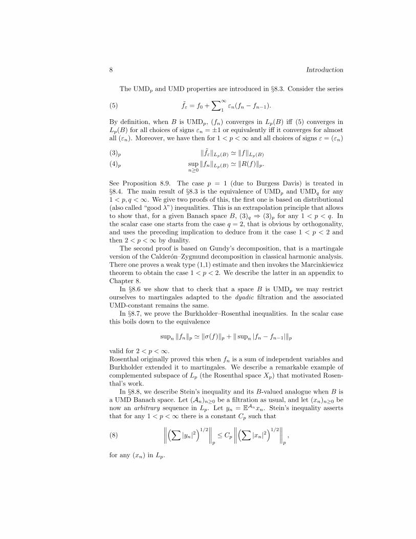
The UMDp and UMD properties are introduced in §8.3. Consider the series

(5) fε = f0 +∑∞

1εn(fn − fn−1).

By definition, when B is UMDp, (fn) converges in Lp(B) iff (5) converges inLp(B) for all choices of signs εn = ±1 or equivalently iff it converges for almostall (εn). Moreover, we have then for 1 < p <∞ and all choices of signs ε = (εn)

‖fε‖Lp(B) ' ‖f‖Lp(B)(3)psupn≥0‖fn‖Lp(B) ' ‖R(f)‖p.(4)p

See Proposition 8.9. The case p = 1 (due to Burgess Davis) is treated in§8.4. The main result of §8.3 is the equivalence of UMDp and UMDq for any1 < p, q <∞. We give two proofs of this, the first one is based on distributional(also called “good λ”) inequalities. This is an extrapolation principle that allowsto show that, for a given Banach space B, (3)q ⇒ (3)p for any 1 < p < q. Inthe scalar case one starts from the case q = 2, that is obvious by orthogonality,and uses the preceding implication to deduce from it the case 1 < p < 2 andthen 2 < p <∞ by duality.

The second proof is based on Gundy’s decomposition, that is a martingaleversion of the Calderon–Zygmund decomposition in classical harmonic analysis.There one proves a weak type (1,1) estimate and then invokes the Marcinkiewicztheorem to obtain the case 1 < p < 2. We describe the latter in an appendix toChapter 8.

In §8.6 we show that to check that a space B is UMDp we may restrictourselves to martingales adapted to the dyadic filtration and the associatedUMD-constant remains the same.

In §8.7, we prove the Burkholder–Rosenthal inequalities. In the scalar casethis boils down to the equivalence

supn ‖fn‖p ' ‖σ(f)‖p + ‖ supn |fn − fn−1|‖p

valid for 2 < p <∞.Rosenthal originally proved this when fn is a sum of independent variables andBurkholder extended it to martingales. We describe a remarkable example ofcomplemented subspace of Lp (the Rosenthal space Xp) that motivated Rosen-thal’s work.

In §8.8, we describe Stein’s inequality and its B-valued analogue when B isa UMD Banach space. Let (An)n≥0 be a filtration as usual, and let (xn)n≥0 benow an arbitrary sequence in Lp. Let yn = EAnxn. Stein’s inequality assertsthat for any 1 < p <∞ there is a constant Cp such that

(8)∥∥∥∥(∑ |yn|2

)1/2∥∥∥∥p

≤ Cp∥∥∥∥(∑ |xn|2

)1/2∥∥∥∥p

,

for any (xn) in Lp.

Introduction 9

For xn in Lp(B), with B UMD the same result remains valid if we replaceon both sides of (8) the expression (

∑|xn|2)1/2 by(∫ ∥∥∥∑ εnxn

∥∥∥2

Bdµ

)1/2

.

See (8.53).In §8.9, we discuss the space BMO and the B-valued version of H1 in the

martingale context. This leads naturally to the atomic version of B-valued H1,denoted by H1

at(B). Its dual can be identified with a BMO-space for B∗-valuedmartingales, at least for a “regular” filtration (An). Equivalently, the spaceH1at(B) can be identified with H1

max(B) that is defined as the completion ofL1(B) with respect to the norm f 7→ E supn ‖fn‖B (here fn = EAnf).

In §8.10, we describe Burkholder’s geometric characterization of UMD spacesin terms of ζ-convexity (Theorem 8.47) but we prefer to give the full details of amore recent result (Theorem 8.48). The latter asserts that a real Banach spaceof the form B = X ⊕X∗ is UMD iff the function

x⊕ ξ → ξ(x)

is the difference of two real valued convex continuous functions on B. Afteran already mentioned first appendix devoted to the Marcinkiewicz theorem,the second one collects several facts (to be used later on) on reverse Holderinequalities. A typical result is that, when 0 < r 0

tpP|z| > t <∞. We

call it reverse Holder because the assumption is boundedness in Lr with r < pand the conclusion is in weak-Lp (or Lp,∞) and a fortiori in Lq for all r < q < p.

In Chapter 9, we give two characterizations of super-reflexive Banach spacesby properties of the underlying metric spaces. The relevant properties involvefinite metric spaces. Given a sequence T = (Tn, dn) of finite metric spaces, wesay that the sequence T embeds Lipschitz uniformly in a metric space (T, d) if forsome constant C there are subsets Tn ⊂ T , and bijective mappings fn : Tn → Tnwith Lipschitz norms satisfying

supn‖fn‖Lip‖f−1

n ‖Lip <∞.

Consider for instance the case when Tn is a finite dyadic tree restricted to itsfirst 1 + 2 + · · · + 2n = 2n+1 − 1 points viewed as a graph and equipped withthe usual geodesic distance. In Theorem 9.1, we prove following [86] that aBanach space B is super-reflexive iff it does not contain the sequence of thesedyadic trees Lipschitz uniformly. More recently (cf. [173]), it was proved thatthe trees can be replaced in this result by the “diamond graphs”. We describethe analogous characterization with diamond graphs in §9.2.

In §9.3, we discuss several non-linear notions of “type p” for metric spaces,notably the notion of Markov type p and we prove the recent result from [212]

10 Introduction

that p-uniformly smooth implies Markov type p. The proof uses martingaleinequalities for martingales naturally associated to Markov chains on finite statespaces.

Acknowledgement I am very grateful to all those who helped me to correctmistakes, misprints and suggested improvements of all kind, in particular JulienGiol, Rostyslav Kravchenko, Javier Parcet, Yanqi Qiu, .....

Chapter 1

Banach space valuedmartingales

1.1 Banach space valued Lp-spaces. Conditionalexpectations

Let (Ω,A,m) be a measure space. Let B be a Banach space. We will denote byF (B) the space of all measurable step functions, i.e. the functions f : Ω → Bfor which there is a partition of Ω, say Ω = A1 ∪ . . . ∪ AN with Ak ∈ A, andelements bk ∈ B such that

(1.1) ∀ω ∈ Ω f(ω) =∑N

11Ak(ω)bk.

Equivalently, F (B) is the space of all measurable functions f : Ω → B takingonly finitely many values.

Definition. We will say that a function f : Ω → B is Bochner measurable ifthere is a sequence (fn) in F (B) tending to f pointwise.

We will denote by L0(Ω,A,m;B) the set of equivalence classes (moduloequality almost everywhere) of Bochner measurable functions.

Let 1 ≤ p ≤ ∞. We will denote by Lp(Ω,A,m;B) the subspace of L0(Ω,A,m)formed of all the functions f such that

∫‖f‖pB dm < ∞ for p < ∞, and

ess sup‖f(·)‖B <∞ for p =∞. We equip this space with the norm

‖f‖Lp(B) =(∫‖f‖pB dm

)1/p

for p <∞

‖f‖L∞(B) = ess sup‖f(·)‖B for p =∞,

with which it becomes a Banach space.

11

12 CHAPTER 1. BANACH SPACE VALUED MARTINGALES

Of course, this definition coincides with the usual one in the scalar valuedcase i.e. if B = R (or C). In that case, we often denote simply by Lp(Ω,A,m)(or sometimes Lp(m), or even Lp) the resulting space of scalar valued functions.

For brievity, we will often write simply Lp(P;B) or, if there is no risk ofconfusion, simply Lp(B) instead of Lp(Ω,A,P;B).

Given ϕ1, . . . , ϕN ∈ Lp and b1, . . . , bN ∈ B we can define a function f : Ω→B in Lp(B) by setting f(ω) =

∑N1 ϕk(ω)bk. We will denote this function by∑N

1 ϕk ⊗ bk and by Lp⊗B the subspace of Lp(B) formed of all such functions.

Proposition 1.1. Let 1 ≤ p <∞.

(i) F (B) ∩ Lp(B) is dense in Lp(B).

(ii) The subspace Lp ⊗B ⊂ Lp(B) is dense in Lp(B).

Proof. Consider f ∈ Lp(B). Let fn ∈ F (B) be such that fn → f pointwise.Then ‖fn(·)‖B → ‖f(·)‖B pointwise, so that if we set gn(ω) = fn(ω)1‖fn‖<2‖f‖we still have gn → f pointwise and in addition sup

n‖gn−f‖ ≤ sup

n‖gn‖+‖f‖ ≤

3‖f‖. Therefore, by dominated convergence, we must have∫‖gn−f‖pB dm→ 0

and of course gn ∈ F (B) ∩ Lp(B). This proves (i). The second point is thenobvious since F (B) ∩ Lp(B) ⊂ Lp ⊗ B (indeed we can take ϕk = 1Ak withm(Ak) <∞, as in (1.1)).

Remark 1.2. If B is finite dimensional, then F (B) is dense in L∞(B) but thisis no longer true in the infinite dimensional case, because the unit ball of B isnot compact.

We now turn to the definition of the integral of a function in L1(B). Considera function f of the form (1.1) in L1(B) ∩ F (B). We define∫

f dm =∑N

1m(Ak)bk.

This defines a continuous linear map from L1(B) ∩ F (B) to B, since we haveobviously by the triangle inequality∥∥∥∥∫ f dm

∥∥∥∥ ≤∑m(Ak)‖bk‖ = ‖f‖L1(B).

By density, this linear map admits an extension defined on the whole of L1(B),that we still denote by

∫f dm when f ∈ L1(B). The extension clearly satisfies

the following fundamental inequality called Jensen’s inequality

(1.2) ∀f ∈ L1(B)∥∥∥∥∫ f dm

∥∥∥∥B

≤∫‖f‖B dm = ‖f‖L1(B).

This extends the linear map f →∫f dm from the scalar valued case to the

B-valued one. More generally: Let (Ω′,A′,m′) be another measure space andlet T : L1(Ω,A,m) → L1(Ω′,A′,m′) be a bounded operator. We may clearly

1.1. B-VALUED LP -SPACES. CONDITIONAL EXPECTATIONS 13

define unambiguously a linear operator T0 : F (B) ∩ L1(m;B) → L1(m′, B) bysetting for any f of the form (1.1)

T0(f) =∑N

1T (1Ak)bk.

We have clearly by the triangle inequality

‖T0(f)‖L1(m′;B) ≤∑N

1‖T (1Ak)‖‖bk‖ ≤ ‖T‖

∑m(Ak)‖bk‖ = ‖T‖‖f‖L1(B).

Thus, we can state

Proposition 1.3. Given a bounded operator T : L1(Ω,A,m)→ L1(Ω′,A′,m′),there is a unique bounded linear map T : L1(Ω,A,m;B) → L1(Ω′,A′,m′;B)such that

(1.3) ∀ϕ ∈ L1(Ω,A,m) ∀b ∈ B T (ϕ⊗ b) = T (ϕ)b.

Moreover, we have ‖T‖ = ‖T‖.

Proof. By the density of F (B) ∩ L1(B) in L1(B), the (continuous) map T0

admits a unique continuous linear extension T from L1(m;B) to L1(m′;B),with ‖T‖ ≤ ‖T0‖ ≤ ‖T‖. If ϕ is a step function in L1, then (1.3) is clear bydefinition of T0. Approximating ϕ in L1 by a step function, we see that (1.3)is true in general. The unicity of T is clear since (1.3) implies that T coincideswith T0 on F (B)∩L1(B). Finally, considering a fixed b with ‖b‖ = 1, we easilyderive from (1.3) that ‖T‖ ≤ ‖T‖, so we obtain ‖T‖ = ‖T‖.

We start by recalling some well known properties of conditional expectations.Let (Ω,A,P) be a probability space and let B ⊂ A be a σ-subalgebra. Theconditional expectation f → EBf is a positive contraction on Lp(Ω,A,P) for all1 ≤ p ≤ ∞. It is characterized by the property

∀h ∈ L∞(Ω,B,P) ∀f ∈ Lp(Ω,A,P)

EB(hf) = hEB(f).

On L2(Ω,A,P), the conditional expectation EB coincides with the orthogonalprojection onto the subspace L2(Ω,B,P).

It is not true in general that a bounded operator on Lp extends boundedlyto Lp(B) as in the preceding Proposition for p = 1. Nervertheless, it is true forpositive operators. The conditional expectation of a vector valued function canbe defined using that fact, as follows.

Proposition 1.4. let 1 ≤ p, q ≤ ∞. Let (Ω,A,P) be an arbitrary measure spaceand let T : Lp(Ω) → Lq(Ω) be a bounded linear operator. Clearly, there is aunique linear operator

T ⊗ IB : Lp(Ω,P)⊗B → Lq(Ω,P)⊗B


such that

∀ϕ ∈ Lp(Ω,P) ∀x ∈ B (T ⊗ IB)(ϕ⊗ x) = T (ϕ)⊗ x.

Now, if T is positive (i.e. if T preserves nonnegative functions) then T ⊗ IBextends to a bounded operator T ⊗ IB from Lp(Ω,P;B) to Lq(Ω,P;B) which hasthe same norm as T , i.e.

‖T ⊗ IB‖Lp(B)→Lq(B) = ‖T‖Lp→Lq .

Proof. It clearly suffices to show that

(1.4) ∀f ∈ Lp(Ω,P)⊗B ‖(T ⊗ IB)f(·)‖Ba.s.≤ T (‖f(·)‖B).

For that purpose, we can assume B separable (or even finite dimensional) sothat there is a countable subset D ⊂ B∗ verifying

∀x ∈ B ‖x‖ = supξ∈D|ξ(x)|.

Clearly for any ξ in B∗ we have

〈ξ, (T ⊗ IB)f(·)〉 = T (〈ξ, f(·)〉)

and hence by the positivity of T for any finite subset D′ ⊂ D

supξ∈D′

|〈ξ, (T ⊗ IB)f(·)〉|a.s.≤ T (sup

ξ∈D|〈ξ, f(·)〉|)

therefore we obtain (1.4) and the proposition follows.

Remark. Let B1 be another Banach space and let u : B → B1 be a boundedoperator. Then for any f in Lp(Ω,A,P;B) we have

˜T ⊗ IB1(u(f)) = u[T ⊗ IB(f)].

In particular, for any ξ in B∗ we have

(1.5) T (ξ(f)) = ξ(T (f)).

Indeed, this is immediately checked for f in Lp(Ω,P)⊗B, and the general caseis obtained after completion.

Note that now that T ⊗ IB makes sense, the preceding argument can berepeated to show that

(1.6) ∀f ∈ Lp(Ω,P;B) ‖(T ⊗ IB)f‖Ba.s.≤ T (‖f(·)‖B).

A priori, in the above (1.6) we implicitly assume that B is a real Banach space,but actually if B is a complex space (and T is C-linear on complex valued L1),we may consider B a fortiori as a real space and then (1.6) remains valid.

1.2. MARTINGALES: BASIC PROPERTIES 15

In particular, the preceding proposition applies for T = EB. For any f inL1(Ω,A,P;B) we will denote again simply by EB(f) the function T ⊗ IB(f) forT = EB. Note that g = EB(f) is characterized by the following properties

(i) g ∈ L1(Ω,B,P;B)

(ii) ∀E ∈ B∫EgdP =

∫EfdP.

Indeed, this is easy to check by ’scalarization’, since it holds in the scalar case.More precisely, a B-valued function g has these properties iff for any ξ in B∗ thescalar valued function 〈ξ, g(·)〉 has similar properties, or equivalently 〈ξ, g(·)〉 =EB〈ξ, f〉, and hence by (1.5) 〈ξ, g〉 = 〈ξ,EBf〉 which means g = EBf as an-nounced.

1.2 Martingales: basic properties

Let B be a Banach space. Let (Ω,A,P) be a probability space. A sequence(Mn)n≥0 in L1(Ω,A,P;B) is called a martingale if there exists an increasingsequence of σ-subalgebras A0 ⊂ A1 ⊂ · · · ⊂ An ⊂ · · · ⊂ A (this is called “afiltration”) such that for each n ≥ 0 Mn is An-measurable and satisfies

Mn = EAn(Mn+1).

For the precise definition of the conditional expectation in the Banach spacevalued case, see the above Proposition 1.4. This implies of course that

∀n < m Mn = EAnMm.

In particular if (Mn) is a B-valued martingale, the above property (ii) (in thepreceding section) yields in the case B = An and n ≤ m

(1.7) ∀n ≤ m ∀A ∈ An∫A

MndP =∫A

MmdP.

A sequence of random variables (Mn) is called adapted to the filtration(An)n≥0 if Mn is An-measurable for each n ≥ 0. Note that the martingaleproperty Mn = EAn(Mn+1) automatically implies that (Mn) is adapted. Ofcourse, the minimal choice of An is simply An = σ(M0,M1, . . . ,Mn).

We will also need the definition of a submartingale. A sequence (Mn)n≥0

of scalar valued random variables in L1 is called a submartingale if there areσ-subalgebras An as above such that Mn is An-measurable and

∀n ≥ 0 Mn ≤ EAnMn+1.

This implies of course that

∀n < m Mn ≤ EAnMm.


More generally, if I is any partially ordered set, then a collection (Mi)i∈I inL1(Ω,P;B) is called a martingale (indexed by I) if there are σ-subalgebrasAi ⊂ A such that Ai ⊂ Aj whenever i < j and Mi = EAiMj .

In particular, whenI = 0,−1,−2, . . .

is the set of all negative integers, the corresponding sequence is usually called areverse martingale.

The following convergence theorem is fundamental.

Theorem 1.5. Let (An) be a fixed increasing sequence of σ-subalgebras of A.Let A∞ be the σ-algebra generated by

⋃n≥0

An. Let 1 ≤ p < ∞ and consider M

in Lp(Ω,P;B). Let us define Mn = EAn(M). Then (Mn)n≥0 is a martingalesuch that Mn → EA∞(M) in Lp(Ω,P;B) when n→∞.

Proof. Note that since An ⊂ An+1 we have EAnEAn+1 = EAn , and similarlyEAnEA∞ = EAn . Replacing M by EA∞M we can assume w.l.o.g. that M isA∞-measurable. We will use the following fact: the union

⋃nLp(Ω,An,P;B)

is dense in Lp(Ω,A∞,P;B). Indeed, let C be the class of all sets A such that1A ∈

⋃nL∞(Ω,An,P), where the closure is meant in Lp(Ω,P) (recall p < ∞).

Clearly C ⊃⋃n≥0

An and C is a σ-algebra hence C ⊃ A∞. This gives the scalar

case version of the above fact. Now, any f in Lp(Ω,A∞,P;B) can be approx-

imated (by definition of the spaces Lp(B)) by functions of the formn∑1

1Aixi

with xi ∈ B and Ai ∈ A∞. But since 1Ai ∈⋃nL∞(Ω,An,P) we clearly have

f ∈⋃nLp(Ω,An,P;B) as announced.

We can now prove Theorem 1.5. Let ε > 0. By the above fact there isan integer k and g in Lp(Ω,Ak,P;B) such that ‖M − g‖p < ε. We have theng = EAng for all n ≥ k, hence

∀n ≥ k Mn −M = EAn(M − g) + g −M

and finally

‖Mn −M‖p ≤ ‖EAn(M − g)‖p + ‖g −M‖p≤ 2ε.

This completes the proof.

Corollary 1.6. In the scalar case (or the f.d. case) every martingale which isbounded in Lp for some 1 ≤ p <∞ and which is uniformly integrable if p = 1 isactually convergent in Lp to a limit M∞ such that Mn = EAnM∞ ∀n ≥ 0.

1.3. EXAMPLES OF FILTRATIONS 17

Proof. Let (Mnk) be a subsequence converging weakly to a limit which we denoteby M∞. Clearly M∞ ∈ Lp(Ω,A∞,P) and we have ∀A ∈ An∫

A

M∞dP = lim∫A

MnkdP,

but whenever nk ≥ n, we have∫AMnkdP =

∫AMndP by the martingale prop-

erty. Hence

∀A ∈ An∫A

M∞dP =∫A

MndP

which forces Mn = EAnM∞. We then conclude by Theorem 1.5 that Mn →M∞in Lp-norm.

Note that conversely any martingale which converges in L1 is clearly uni-formly integrable.

Remark 1.7. Fix 1 ≤ p < ∞. Let I be a directed set, with order denotedsimply by ≤. This means that for any pair i, j in I there is k ∈ I such thati ≤ k and j ≤ k. Let (Ai) be a family of σ-algebras directed by inclusion (i.e.we have Ai ⊂ Aj whenever i ≤ j). The extension of the notion of martingaleis obvious: A collection of random variables (fi)i∈I in Lp(B) will be called amartingale if fi = EAi(fj) holds whenever i ≤ j. The resulting net convergesin Lp(B) iff for any increasing sequence i1 ≤ · · · ≤ in ≤ in+1 ≤ · · · , the (usualsense) martingale (fin) converges in Lp(B). Indeed, this merely follows from

the metrizability of Lp(B) ! More precisely, if we assume that σ( ⋃i∈IAi)

= A,

then for any f in Lp(Ω,A,P;B), the directed net (EAif)i∈I converges to f inLp(B). Indeed, this net must satisfy the Cauchy criterion, because otherwise wewould be able for some δ > 0 to construct (by induction) an increasing sequencei(1) ≤ i(2) ≤ . . . in I such that ‖EAi(k)f − EAi(k−1)f‖Lp(B) > δ for all k > 1,and this would then contradict Theorem 1.5. Thus, EAif converges to a limitF in Lp(B), and hence for any set A ⊂ Ω in

⋃j∈IAj we must have

∫A

f = limi

∫A

EAif =∫A

F.

Since the equality∫Af =

∫AF must remain true on the σ-algebra generated by⋃

Aj , we conclude that f = F , thus completing the proof that EAif → f inLp(B).

1.3 Examples of filtrations

The most classical example of filtration is the one associated to a sequenceof independent (real valued) random variables (Yn)n≥1 on a probability space(Ω,A,P). Let An = σ(Y1, . . . , Yn) for all n ≥ 1 and A0 = φ,Ω. In that case,a sequence of random variables (fn)n≥0 is adapted to the filtration (An)n≥0 iff


f0 is constant and, for each n ≥ 1, fn depends only on Y1, . . . , Yn, i.e. there isa (Borel measurable) function Fn on Rn such that

fn = Fn(Y1, . . . , Yn).

The martingale condition can then be written as

∀n ≥ 0 Fn(Y1, . . . , Yn) =∫Fn+1(Y1, . . . , Yn, y) dPn(y)

where Pn is the probability distribution (or “the law”) of Yn+1.An equivalent but more “intrinsic” model arises when one considers Ω = RN∗

equipped with the product probability measure P =⊗

n≥1 Pn. If one denotesby Y = (Yn)n≥1 a generic point in Ω, the random variable Y → Yn appears asthe n-th coordinate, and Y → Fn(Y ) is An-measurable iff Fn(Y ) depends onlyon the n first coordinates of Y .

The dyadic filtration (Dn)n≥0 on D = −1, 1N∗ is the fundamental exampleof this kind: Here we denote by

εn : D → −1, 1 (n = 1, 2, . . .)

the n-th coordinate, we equip D with the probability measure

µ = ⊗(δ1 + δ−1)/2,

and we set Dn = σ(ε1, . . . , εn), D0 = φ,D.Clearly, the variables (εn) are independent on (D,D, µ) and take the values ±1with equal probability 1/2.Note thatDn admits exactly 2n atoms and moreover dimL2(D,Dn, µ) = 2n. Forany finite subset A ⊂ [1, 2, . . .], let wA =

∏n∈A

εn with the convention wφ ≡ 1.

It is easy to check that wA | A ⊂ [1, . . . , n] (resp. wA | |A| < ∞) is anorthonormal basis of L2(D,Dn, µ) (resp. L2(D,D, µ)).Given a Banach space B, a B-valued martingale fn : D → B adapted to thedyadic filtration (Dn) is caracterized by the property that

∀n ≥ 1 (fn − fn−1)(ε1, . . . , εn) = εnϕn−1(ε1, . . . , εn−1),

where ϕn−1 depends only on ε1, . . . , εn−1. We leave the easy verification of thisto the reader.Of course the preceding remarks remain valid if one works with any sequence of±1-valued independent random variables (εn) such that P(εn = ±1) = 1/2 onan “abstract” probability space (Ω,P).

In classical analysis, it is customary to use the Rademacher functions (rn)n≥1

on the Lebesgue interval ([0, 1], dt) instead of (εn). We need some notation tointroduce these. Given an interval I ⊂ R we divide I into parts of equal lengthand we denote by I+ and I− respectively the left and right half of I. Notethat we do not specify whether the end points belong to I since the latter arenegligible for the Lebesgue measure on [0, 1] (or [0, 1[ or R). Let

hI = 1I+ − 1I− .

1.3. EXAMPLES OF FILTRATIONS 19

We denote I1(1) = [0, 1[, I2(1) = [0, 12 [, I2(2) =

[12 , 1[ and more generally

In(k) =[k − 12n−1

,k

2n−1

[for k = 1, 2, . . . , 2n−1 (n ≥ 1).We then set h1 ≡ 1, h2 = hI1(1), h3 =

√2 hI2(1), h4 =

√2 hI2(2) and more

generally

∀n ≥ 1 ∀k = 1, . . . , 2n−1 h2n−1+k = |In(k)|−1/2hIn(k).

Note that ‖hn‖2 = 1 for all n ≥ 1.The Rademacher function rn can be defined, for each n ≥ 1, by

rn =∑2n−1

k=1hIn(k).

Then the sequence (rn)n≥1 has the same distribution on ([0, 1], dt) as the se-quence (εn)n≥1 on (D,µ). Let An = σ(r1, . . . , rn). Then An is generated bythe 2n-atoms In+1(k) | 1 ≤ k ≤ 2n, each having length 2−n. The dimensionof L2([0, 1],An) is 2n and the functions h1, . . . , h2n (resp. hn | n ≥ 1) forman orthonormal basis of L2([0, 1],An) (resp. L2([0, 1])).

The “Haar filtration” (Bn)n≥1 on [0, 1] is defined by

Bn = σ(h1, . . . , hn),

so that we have σ(h1, . . . , h2n) = σ(r1, . . . , rn) or equivalently B2n = An for alln ≥ 1 (note that here B1 is trivial). It is easy to check that Bn is an atomicσ-algebra, with exactly n atoms. Since the conditional expectation EBn is theorthogonal projection from L2 to L2(Bn), we have for any f in L2([0, 1])

∀n ≥ 1 EBnf =∑n

1〈f, hk〉hk

and hence for all n ≥ 2

(1.8) EBnf − EBn−1f = 〈f, hn〉hn.

More generally for any B-valued martingale (fn)n≥∅ adapted to (Bn)n≥1 wehave

∀n ≥ 2 fn − fn−1 = hnxn

for some sequence (xn) in B. The Haar functions are in some sense the firstexample of wavelets (see e.g. [64]). Indeed, if we set

h = 1[0, 12 [ − 1[ 12 ,1[

(this is the same as the function previously denoted by h2), then the system offunctions

(1.9)

2m2 h((t+ k)2m) | k,m ∈ Z

is an orthonormal basis of L2(R). Note that the constant function 1 is not inL2(R).

In the system (1.9), the sequence hn | n ≥ 1 coincides with the subsystemformed of all functions in (1.9) with support included in [0, 1].


1.4 Almost sure convergence and maximal in-equalities

To handle the a.s. convergence of martingales, we will need (as usual) theappropriate maximal inequalities. In the martingale case, these are Doob’sinequalities. Their proof uses stopping times which are a basic tool in martingaletheory. Given an increasing sequence (An)n≥0 of σ-subalgebras on Ω, a randomvariable T : Ω→ N ∪ ∞ is called a stopping time if

∀n ≥ 0 T ≤ n ∈ An,

or equivalently if∀n ≥ 0 T = n ∈ An.

If T <∞ a.s., then T is called a finite stopping time.

Proposition 1.8. For any martingale (Mn)n≥0 relative to (An)n≥0 and forevery stopping time T , let us denote by Mn∧T the variable Mn∧T (ω)(ω). Then(Mn∧T )n≥0 is a martingale relative to (An)n≥0.

Proof. Observe that Mn∧T clearly is in L1 (since Mn is always assumed in L1).Moreover, we have

Mn∧T −M(n−1)∧T = 1n≤T(Mn −Mn−1),

but n ≤ Tc = T < n ∈ An−1 hence

EAn−1(Mn∧T −M(n−1)∧T ) = 1n≤TEAn−1(Mn −Mn−1) = 0.

Given a stopping time T , we can define the associated σ-algebra AT asfollows: we say that a set A in A belongs to AT if A ∩ T ≤ n belongs to Anfor each n ≥ 0. Then AT is a σ-algebra.

Exercises. (i) Consider M∞ in L1(Ω,A,P;B) and let Mn = EAnM∞ be theassociated martingale. Then if T is a stopping time, we have

MT = EAT (M∞).

Moreover,

(1.10) EAn(MT ) = MT∧n = EAT (Mn).

More generally, if S is any other stopping time, T ∧ S and T ∨ S are stoppingtimes and we have

EAS (MT ) = MT∧S = EAT (MS).

(ii) If (Mn)n≥0 is a martingale in L1(Ω,A,P;B) and if T0 ≤ T1 ≤ . . . is asequence of bounded stopping times then (MTk)k≥0 is a martingale relative tothe sequence of σ-algebras AT0 ⊂ AT1 ⊂ · · · . This also holds for unboundedtimes if we assume as in (i) that (Mn)n≥0 converges in L1(Ω,A,P;B).

1.4. ALMOST SURE CONVERGENCE. MAXIMAL INEQUALITIES 21

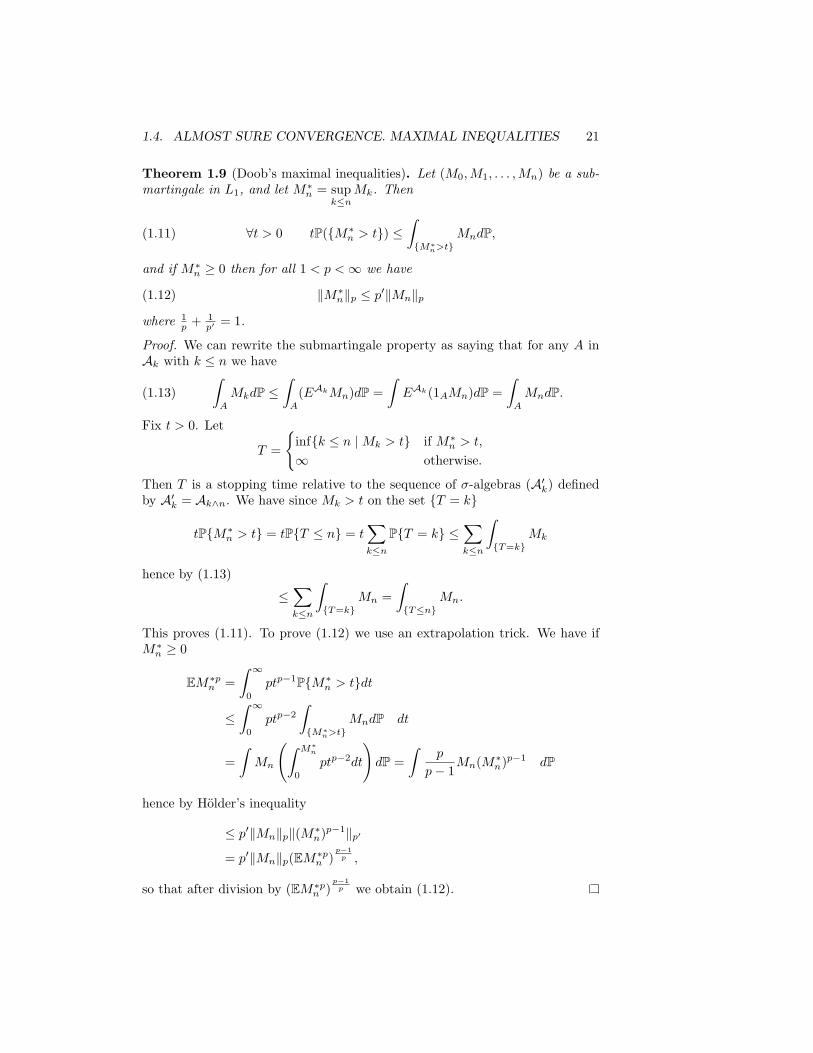
Theorem 1.9 (Doob’s maximal inequalities). Let (M0,M1, . . . ,Mn) be a sub-martingale in L1, and let M∗n = sup

k≤nMk. Then

(1.11) ∀t > 0 tP(M∗n > t) ≤∫M∗n>t

MndP,

and if M∗n ≥ 0 then for all 1 < p <∞ we have

(1.12) ‖M∗n‖p ≤ p′‖Mn‖p

where 1p + 1

p′ = 1.

Proof. We can rewrite the submartingale property as saying that for any A inAk with k ≤ n we have

(1.13)∫A

MkdP ≤∫A

(EAkMn)dP =∫EAk(1AMn)dP =

∫A

MndP.

Fix t > 0. Let

T =

infk ≤ n |Mk > t if M∗n > t,∞ otherwise.

Then T is a stopping time relative to the sequence of σ-algebras (A′k) definedby A′k = Ak∧n. We have since Mk > t on the set T = k

tPM∗n > t = tPT ≤ n = t∑k≤n

PT = k ≤∑k≤n

∫T=k

Mk

hence by (1.13)

≤∑k≤n

∫T=k

Mn =∫T≤n

Mn.

This proves (1.11). To prove (1.12) we use an extrapolation trick. We have ifM∗n ≥ 0

EM∗pn =∫ ∞

0

ptp−1PM∗n > tdt

≤∫ ∞

0

ptp−2

∫M∗n>t

MndP dt

=∫Mn

(∫ M∗n

0

ptp−2dt

)dP =

∫p

p− 1Mn(M∗n)p−1 dP

hence by Holder’s inequality

≤ p′‖Mn‖p‖(M∗n)p−1‖p′

= p′‖Mn‖p(EM∗pn )p−1p ,

so that after division by (EM∗pn )p−1p we obtain (1.12).


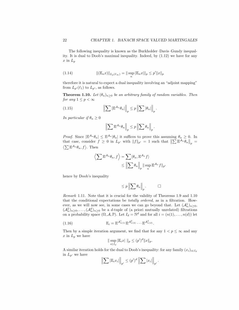
The following inequality is known as the Burkholder–Davis–Gundy inequal-ity. It is dual to Doob’s maximal inequality. Indeed, by (1.12) we have for anyx in Lp

(1.14) ‖(Enx)‖Lp(`∞) = ‖ supn|Enx|‖p ≤ p′‖x‖p

therefore it is natural to expect a dual inequality involving an “adjoint mapping”from Lp′(`1) to Lp′ , as follows.

Theorem 1.10. Let (θn)n≥0 be an arbitrary family of random variables. Thenfor any 1 ≤ p <∞

(1.15)∥∥∥∑ |EAnθn|

∥∥∥p≤ p

∥∥∥∑ |θn|∥∥∥p.

In particular if θn ≥ 0 ∥∥∥∑EAnθn∥∥∥p≤ p

∥∥∥∑ θn

∥∥∥p.

Proof. Since |EAnθn| ≤ EAn |θn| it suffices to prove this assuming θn ≥ 0. Inthat case, consider f ≥ 0 in Lp′ with ‖f‖p′ = 1 such that

∥∥∑EAnθn∥∥p

=⟨∑EAnθn, f

⟩. Then⟨∑

EAnθn, f⟩

=∑〈θn,EAnf〉

≤∥∥∥∑ θn

∥∥∥p‖ sup

nEAnf‖p′

hence by Doob’s inequality

≤ p∥∥∥∑ θn

∥∥∥p.

Remark 1.11. Note that it is crucial for the validity of Theorems 1.9 and 1.10that the conditional expectations be totally ordered, as in a filtration. How-ever, as we will now see, in some cases we can go beyond that. Let (A1

n)n≥0,(A2

n)n≥0, . . . , (Adn)n≥0 be a d-tuple of (a priori mutually unrelated) filtrationson a probability space (Ω,A,P). Let Id = Nd and for all i = (n(1), . . . , n(d)) let

(1.16) Ei = EA1n(1)EA

2n(2) · · ·EA

dn(d) .

Then by a simple iteration argument, we find that for any 1 < p ≤ ∞ and anyx in Lp we have

‖ supi∈Id|Eix| ‖p ≤ (p′)d‖x‖p.

A similar iteration holds for the dual to Doob’s inequality: for any family (xi)i∈Idin Lp′ we have ∥∥∥∑ |Eixi|

∥∥∥p′≤ (p′)d

∥∥∥∑ |xi|∥∥∥p′.


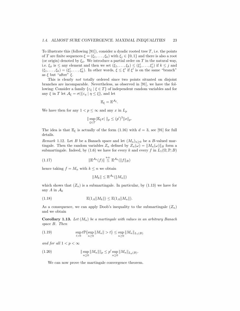
To illustrate this (following [91]), consider a dyadic rooted tree T , i.e. the pointsof T are finite sequences ξ = (ξ1, . . . , ξk) with ξj ∈ 0, 1 and there is also a root(or origin) denoted by ξφ. We introduce a partial order on T in the natural way,i.e. ξφ is ≤ any element and then we set (ξ1, . . . , ξk) ≤ (ξ′1, . . . , ξ

′j) if k ≤ j and

(ξ1, . . . , ξk) = (ξ′1, . . . , ξ′k). In other words, ξ ≤ ξ′ if ξ′ is on the same “branch”

as ξ but “after” ξ.This is clearly not totally ordered since two points situated on disjoint

branches are incomparable. Nevertheless, as observed in [91], we have the fol-lowing: Consider a family εξ | ξ ∈ T of independent random variables and forany ξ in T let Aξ = σ(εη | η ≤ ξ, and let

Eξ = EAξ .

We have then for any 1 < p ≤ ∞ and any x in Lp

‖ supξ∈T|Eξx| ‖p ≤ (p′)3‖x‖p.

The idea is that Eξ is actually of the form (1.16) with d = 3, see [91] for fulldetails.

Remark 1.12. Let B be a Banach space and let (Mn)n≥0 be a B-valued mar-tingale. Then the random variables Zn defined by Zn(ω) = ‖Mn(ω)‖B form asubmartingale. Indeed, by (1.6) we have for every k and every f in L1(Ω,P;B)

(1.17) ‖EAk(f)‖a.s.≤ EAk(‖f‖B)

hence taking f = Mn with k ≤ n we obtain

‖Mk‖ ≤ EAk(‖Mn‖)

which shows that (Zn) is a submartingale. In particular, by (1.13) we have forany A in Ak

(1.18) E(1A‖Mk‖) ≤ E(1A‖Mn‖).

As a consequence, we can apply Doob’s inequality to the submartingale (Zn)and we obtain

Corollary 1.13. Let (Mn) be a martingale with values in an arbitrary Banachspace B. Then

(1.19) supt>0

tPsupn≥0‖Mn‖ > t ≤ sup

n≥0‖Mn‖L1(B)

and for all 1 < p <∞

(1.20) ‖ supn≥0‖Mn‖‖p ≤ p′ sup

n≥0‖Mn‖Lp(B).

We can now prove the martingale convergence theorem.


Theorem 1.14. Let 1 ≤ p <∞. Let B be an arbitrary Banach space. Considerf in Lp(Ω,A,P;B) and let Mn = EAn(f) be the associated martingale. ThenMn converges a.s. to EA∞(f). Therefore, if a martingale (Mn) is convergent inLp(Ω,P;B) to a limit M∞, then it necessarily converges a.s. to this limit, andwe have Mn = EAnM∞ for all n ≥ 0.

Proof. The proof is based on a general principle, going back to Banach, thatallows us to deduce almost sure convergence results from suitable maximalinequalities. By Theorem 1.5, we know that EAn(f) converges in Lp(B) toM∞ = EA∞(f). Fix ε > 0 and choose k so that supn≥k ‖Mn −Mk‖Lp(B) < ε.We will apply (1.19) and (1.20) to the martingale (M ′n)n≥0 defined by

M ′n = Mn −Mk if n ≥ k and M ′n = 0 if n ≤ k.

We have in the case 1 0

tPsupn≥k‖Mn −Mk‖ > t ≤ ε.

Therefore if we define pointwise

` = limk→∞

supn,m≥k

‖Mn −Mm‖

we have` = inf

k≥0supn,m≥k

‖Mn −Mm‖ ≤ 2 supn≥k‖Mn −Mk‖.

Hence we find ‖`‖p ≤ 2p′ε and

supt>0

tP` > 2t ≤ ε,

which implies (since ε > 0 is arbitrary) that ` = 0 a.s., and hence by theCauchy criterion that (Mn) converges a.s. Since Mn → M∞ in Lp(B) we havenecessarily Mn → M∞ a.s. Note that if a martingale Mn tends to a limit M∞in Lp(B) then necessarily Mn = EAn(M∞). Indeed, Mn = EAnMm for allm ≥ n and by continuity of EAn we have EAnMm → EAnM∞ in Lp(B) so thatMn = EAnM∞ as announced. This settles the last assertion.

Corollary 1.15. Every scalar valued martingale (Mn)n≥0 which is bounded inLp for some p > 1 (resp. uniformly integrable) must converge a.s. and in Lp(resp. L1).

Proof. By Corollary 1.6, if (Mn)n≥0 is bounded in Lp for some p > 1 (resp.uniformly integrable) then Mn converges in Lp (resp. L1) and by Theorem 1.14the a.s. convergence is then automatic.


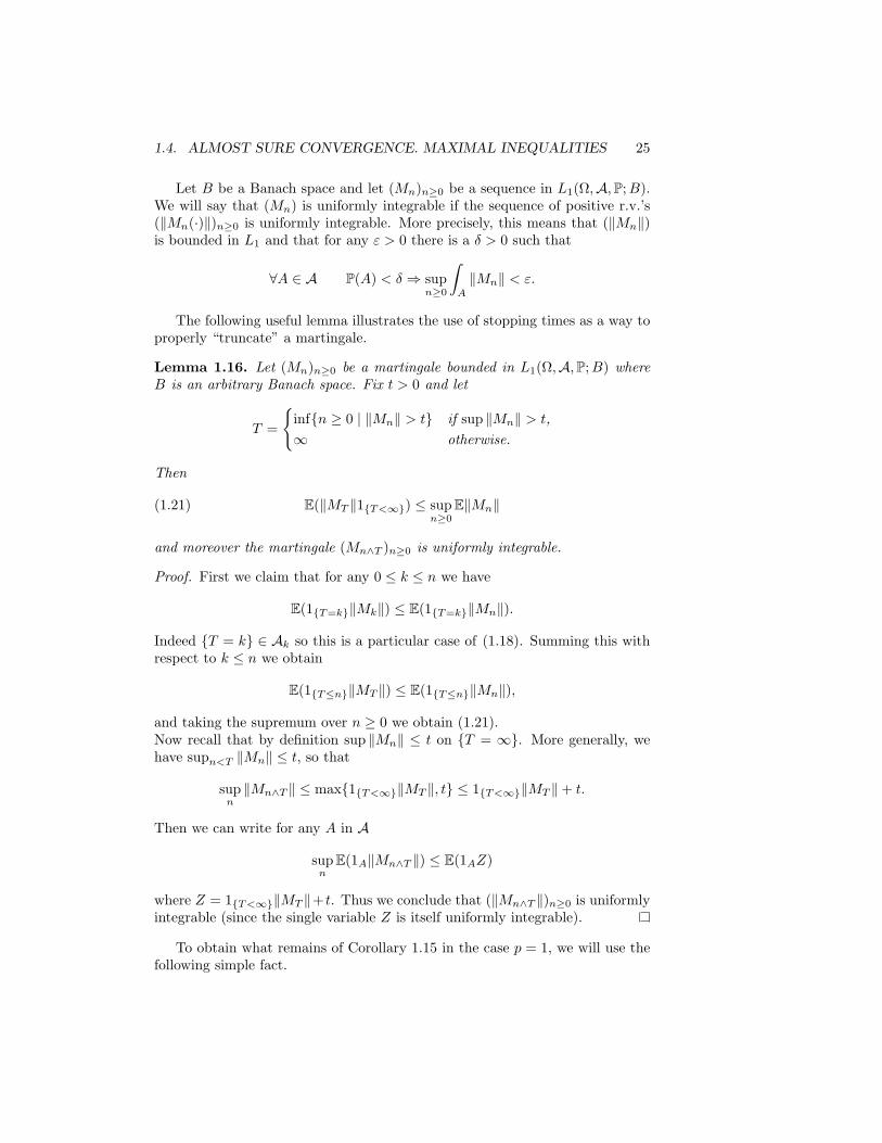
Let B be a Banach space and let (Mn)n≥0 be a sequence in L1(Ω,A,P;B).We will say that (Mn) is uniformly integrable if the sequence of positive r.v.’s(‖Mn(·)‖)n≥0 is uniformly integrable. More precisely, this means that (‖Mn‖)is bounded in L1 and that for any ε > 0 there is a δ > 0 such that

∀A ∈ A P(A) < δ ⇒ supn≥0

∫A

‖Mn‖ < ε.

The following useful lemma illustrates the use of stopping times as a way toproperly “truncate” a martingale.

Lemma 1.16. Let (Mn)n≥0 be a martingale bounded in L1(Ω,A,P;B) whereB is an arbitrary Banach space. Fix t > 0 and let

T =

infn ≥ 0 | ‖Mn‖ > t if sup ‖Mn‖ > t,∞ otherwise.

Then

(1.21) E(‖MT ‖1T<∞) ≤ supn≥0

E‖Mn‖

and moreover the martingale (Mn∧T )n≥0 is uniformly integrable.

Proof. First we claim that for any 0 ≤ k ≤ n we have

E(1T=k‖Mk‖) ≤ E(1T=k‖Mn‖).

Indeed T = k ∈ Ak so this is a particular case of (1.18). Summing this withrespect to k ≤ n we obtain

E(1T≤n‖MT ‖) ≤ E(1T≤n‖Mn‖),

and taking the supremum over n ≥ 0 we obtain (1.21).Now recall that by definition sup ‖Mn‖ ≤ t on T = ∞. More generally, wehave supn<T ‖Mn‖ ≤ t, so that

supn‖Mn∧T ‖ ≤ max1T<∞‖MT ‖, t ≤ 1T<∞‖MT ‖+ t.

Then we can write for any A in A

supn

E(1A‖Mn∧T ‖) ≤ E(1AZ)

where Z = 1T<∞‖MT ‖+ t. Thus we conclude that (‖Mn∧T ‖)n≥0 is uniformlyintegrable (since the single variable Z is itself uniformly integrable).

To obtain what remains of Corollary 1.15 in the case p = 1, we will use thefollowing simple fact.


Proposition 1.17. Let (Ω,A,P) be a probability space. Let B be a Banachspace and let (An)n≥0 be an increasing sequence of σ-subalgebras of A. Thefollowing are equivalent:

(i) Every B-valued martingale adapted to (An)n≥0 and bounded in L1(Ω,P;B)is a.s. convergent.

(ii) Every B-valued uniformly integrable martingale adapted to (An)n≥0 is a.s.convergent.

Proof. Assume (ii). Let (Mn) be a martingale bounded in L1(B). Fix t > 0and consider (Mn∧T ) as in Lemma 1.16. Since (Mn∧T ) is uniformly integrable,it converges a.s. by (ii). This implies that if T (ω) =∞ then (Mn(ω))n≥0 isa.s. convergent. But by Doob’s inequalities

PT <∞ = Psup ‖Mn‖ > t ≤ C

t

where C = sup E‖Mn‖. Therefore this probability can be made arbitrarilysmall by choosing t large, so that we conclude that the martingale (Mn)n≥0

itself converges a.s. This shows that (ii) ⇒ (i). The converse is trivial.

Finally, we can state what is usually referred to as the “martingale conver-gence theorem”.

Theorem 1.18. Every L1-bounded scalar valued martingale converges a.s.

Proof. By Corollary 1.6, every scalar valued uniformly integrable martingaleconverges in L1, and hence by Theorem 1.14 it converges a.s. Thus the presentstatement follows from the implication (ii) ⇒ (i) from Proposition 1.17.

We will also need the following

Theorem 1.19. Every submartingale (Mn) bounded in L1 (resp. and uniformlyintegrable) converges a.s. (resp. and in L1.)

Proof. We use the so-called Doob decomposition: we will write our submartin-gale as the sum of a martingale (Mn)n≥0 and a predictable increasing se-quence (An) (recall that this means that An is An−1 measurable for eachn ≥ 1). Let us write ∆0 = M0 and ∆n = Mn − Mn−1 if n ≥ 1. Letdn = ∆n − EAn−1(∆n) if n ≥ 1 and d0 = ∆0, and let Mn =

∑k≤n

dk. Then

(Mn)n≥0 is a martingale. Indeed, by construction we have EAn−1(dn) = 0 orequivalently EAn−1Mn = Mn−1. To relate (Mn) to (Mn), we note that

Mn =∑

0≤k≤n

∆k =∑

0≤k≤n

dk +∑

1≤k≤n

EAk−1(∆k)

henceMn = Mn +An


whereAn =

∑1≤k≤n

EAk−1(∆k).

Moreover, by the submartingale property EAn−1(∆n) ≥ 0 for all n ≥ 1 so that

0 ≤ A1 ≤ A2 ≤ · · · ≤ An−1 ≤ An ≤ · · · .

On one hand, EAn =∑

1≤k≤nE∆k = EMn − EM0, and since (Mn) is assumed

bounded in L1 we have supn≥1

EAn <∞. Therefore by monotonicity An converges

a.s. and in L1 when n→∞ (in particular it is a uniformly integrable sequence).On the other hand, we have

E|Mn| = E|Mn −An| ≤ E|Mn|+ EAn

therefore (Mn) also is bounded in L1 and is uniformly integrable if (Mn) is. Bythe martingale convergence theorem (Theorem 1.18) (Mn) converges a.s. henceMn = Mn +An also converges a.s. and, in the uniformly integrable case, it alsoconverges in L1.

If we impose the initial condition A0 = 0, the above proof also shows unique-ness: Indeed, Mn = Mn+An implies An−An−1 = ∆n−dMn and (assuming Ann− 1-measurable) this imposes An −An−1 = EAn−1(∆n − dMn) = EAn−1(∆n)which uniquely determines An if set A0 = 0.

Corollary 1.20. Let B be an arbitrary Banach space and let (Mn)n≥0 be aB-valued martingale bounded in L1(B). Then ‖Mn‖B converges a.s. Moreover,(Mn)n≥0 converges a.s. in norm iff Mn(ω) | n ≥ 0 is relatively compact foralmost all ω.

Proof. The first assertion follows from Theorem 1.19 and Remark 1.12. It suf-fices to prove the second one for a separable B. Assume that Mn(ω) | n ≥ 0 isω-a.s. relatively compact. Let f(ω) be a cluster point in B of Mn(ω) | n ≥ 0.Note that by Theorem 1.18 for any ξ in B∗, ξ(Mn(ω)) converges ω-a.s., andhence it must converge to ξ(f(ω)). (Incidentally: this shows that f is scalarlymeasurable, and hence by Appendix 2 is Bochner measurable). Let D ⊂ B∗

be a countable weak-∗ dense subset. Clearly, Mn(ω) tends ω-a.s. to f(ω) inthe σ(B,D)-topology, but if Mn(ω) | n ≥ 0 is relatively compact, the lattertopology coincides on it with the norm topology, and hence Mn(ω) → f(ω) innorm. Conversely, if Mn(ω) | n ≥ 0 is convergent it is obviously relativelycompact.

Remark 1.21. The maximal inequalities for B-valued martingales can be con-siderably strengthened when B = `r for some 1 < r < ∞: Consider a fil-tration (An) as usual, f ∈ Lp(`r) and let (fn) be the martingale associatedto f . Let (ek) be the canonical basis of `r. We may develop f and fn as


f =∑k f(k)ek and fn =

∑k fn(k)ek. In accordance with previous notation,

we set f(k)∗ = supn |fn(k)|. Let then

f∗∗ = ‖∑

f(k)∗ek‖`r = (∑

f(k)∗r)1/r.

Then, for any 1 < p <∞, there is a constant c(p, r) such that

‖f∗∗‖p ≤ c(p, r)‖f‖Lp(`r) = c(p, r)‖(∑|f(k)|r)1/r‖p.

Note that p = r is an easy consequence of Doob’s inequality. See [56] for p ≤ rand [187] for the general case and for a weak type-(1, 1) inequality that can beproved using the Gundy decomposition described in the next chapter. Finally,the extension to the case B = Lr requires only minor modifications.

There are cases where the maximal inequalities can be extended to Lp with0 < p < 1. For instance, let (Yn)n≥0 be a sequence of independent B-valuedrandom variables, let fn =

∑n0 Yn. If Yn ∈ L1(B) is symmetric for all n (this

implies EYn = 0), then (fn)n≥0 is a martingale satisfying P(supn‖fn‖ > t) ≤

2 supn

P(‖fn‖ > t). More generally, we quote without proof the following:

Theorem 1.22. Let (Yn) be a sequence of B-valued random variables, such that,for any choice of signs ξn = ±1, the sequence (ξnYn) has the same distributionas (Yn). Let fn =

∑n0 Yk. We have then:

∀t > 0 P(sup ‖fn‖ > t) ≤ 2 lim sup P(‖fn‖ > t)(1.22)∀p > 0 E sup ‖fn‖p ≤ 2 lim sup E‖fn‖p.(1.23)

If fn converges to a limit f∞ in probability (i.e. ‖fn − f∞‖ → 0 in probability),then it actually converges a.s. In particular, if fn converges in Lp (p > 0), thenit automatically converges a.s. Finally, if fn converges a.s. to a limit f∞, wehave

(1.24) ∀t > 0 P(sup ‖fn‖ > t) ≤ 2P(‖f∞‖ > t).

More generally for any Borel convex subset K ⊂ B, we have

P(∪nfn 6∈ K) ≤ 2P(f∞ 6∈ K).

Corollary 1.23. Let (Yn) be independent variables in L1(B) with mean zero(i.e. EYn = 0) and let fn =

∑n0 Yk as before. Then, for any p ≥ 1, we have

‖ sup ‖fn‖‖p ≤ 21+1/p sup ‖fn‖Lp(B).

Proof. Let (Y ′n)n be an independent copy of the sequence (Yn), let Yn = Yn−Y ′nand f ′n =

∑n0 Y′n. Note that (Yn) are independent and symmetric. By (1.23) we

haveE sup ‖fn‖p ≤ 2 sup E‖fn‖p


but now if p ≥ 1 we have by convexity

E sup ‖fn‖p = E sup ‖fn − Ef ′n‖p ≤ E sup ‖fn − f ′n‖p

≤ 2 sup E‖fn − f ′n‖p

≤ 2 sup E(‖fn‖+ ‖f ′n‖)p

≤ 2p(E sup ‖fn‖p + E sup ‖f ′n‖p) = 2p+1E sup ‖fn‖p.

Corollary 1.24. For a series of independent B-valued random variables, con-vergence in probability implies almost sure convergence.

Proof. Let fn =∑n

0 Yk, with (Yk) independent. Let (Y ′k) be an independentcopy of the sequence (Yk) and let f ′n =

∑n0 Y′k. Then the variables (Yk − Y ′k)

are independent and symmetric. If fn converges in probability (when n→∞),then obviously f ′n and hence fn − f ′n also does. By the preceding Theorem,fn − f ′n converges a.s., therefore we can choose fixed values xn = f ′n(ω0) suchthat fn − xn converges a.s.. A fortiori, fn − xn converges in probability, andsince fn also does, the difference fn − (fn − xn) = xn also does, which meansthat (xn) is convergent in B. Thus the a.s. convergence of fn− xn implies thatof fn.

Remark 1.25. There are well known counterexamples showing that Theorem 1.18does not extend to the Banach space valued case. For instance, let Ω = −1, 1Nequipped with the usual probability measure P and let An be the σ-algebragenerated by the (n+ 1) first coordinates denoted by ε0, ε1, . . . , εn. A classicalexample of a real valued martingale is Mn =

∏k≤n

(1 + εk), which is positive and

of integral 1. Note however that it does not converge in L1. Another exampleis Mn =

∑k≤n

αkεk where (αk) are real coefficients. This particular martingale is

bounded in L1 iff Σ|αn|2 is finite. By the martingale convergence theorem, thesetwo martingales must converge a.s. However, we can give very similar Banachspace valued examples which do not converge. Take for instance B = c0 andlet (en) be the canonical basis of c0. Let M1

n =∑k≤n

εkek. Then ‖M1n(ω)‖c0 =

supk≤n|εk(ω)| ≡ 1 but clearly there is no point ω in −1, 1N such that the sequence

(M1n(ω))n≥0 is convergent in c0, since we have

∀ω ∈ Ω ∀k < n ‖M1n(ω)−M1

k (ω)‖B = 1.

We can give a similar example in L1. Let B = L1(Ω,P) itself and let

(1.25) M2n(ω) =

∏k≤n

(1 + εk(ω)εk).

Then again ‖M2n(ω)‖B = 1 for all ω, but also it is easy to check that

∀ω ∈ Ω ∀k < n ‖M2n(ω)−M2

k (ω)‖B ≥ 1, and ‖M2n(ω)−M2

n−1(ω)‖B = 1,


so that (M2n)n≥0 is nowhere convergent.

In the next chapter, we will show that the preceding examples cannot occurin a Banach space with the RNP.

1.5 Reverse martingales

We will prove here the following

Theorem. Let B be an arbitrary Banach space. Let (Ω,A,P) be a probabilityspace and let A0 ⊃ A−1 ⊃ A−2 ⊃ · · · be a (this time decreasing) sequence ofσ-subalgebras of A. Let A−∞ =

⋂n≥0

A−n. Then for any f in Lp(Ω,A, P ;B),

with 1 ≤ p < ∞, the reverse martingale (EA−n(f))n≥0 converges to EA−∞(f)a.s. and in Lp(B).

We first check the convergence in Lp(B). Since the operators (EA−n)n≥0

are equicontinuous on Lp(B) it suffices to check this for f in a dense subset of

Lp(B). In particular, it suffices to consider f of the form f =n∑1ϕixi with ϕi

an indicator function and xi in B. Since ϕi ∈ L2(Ω,P), we have (by classicalHilbert space theory) EA−nϕi → EA−∞ϕi in L2(Ω,P) when n→∞. (Note thatL2(Ω,A−∞,P) is the intersection of the family (L2(Ω,A−n,P))n≥0.)Observe that ‖f − g‖p ≤ ‖f − g‖2 if p ≤ 2 and ‖f − g‖pp ≤ 2p−2‖f − g‖22if ‖f‖∞ ≤ 1, ‖g‖∞ ≤ 1 and p > 2. Using this, we obtain that, a fortiori,EA−nf → EA−∞f in Lp(B) for every f of the above form, and hence for everyf in Lp(B).

We now turn to a.s. convergence. We first replace f by f = f − EA−∞(f)so that we can assume EA−n(f) → 0 in Lp(B) and a fortiori in L1(B). Letfn = EA−nf . Now fix n > 0 and k > 0 and consider the (ordinary sense)martingale

Mj =f−n−k+j for j = 0, 1, . . . , k,f−n if j ≥ k.

Then by Doob’s inequality (1.19) applied to (Mj) we have for all t > 0

tP supn≤m≤n+k

‖f−m‖ > t ≤ E‖f−n‖

thereforetP sup

m≥n‖f−m‖ > t ≤ E‖f−n‖

and since E‖f−n‖ → 0 when n → ∞, we have supm≥n‖f−m‖ → 0 a.s., or equiva-

lently f−n → 0 a.s. when n→∞. As a corollary, we have the following classical application to the strong law

of large numbers.

1.6. NOTES AND REMARKS 31

Corollary. Let ϕ1, . . . , ϕn be a sequence of independent, identically distributedrandom variables in L1(Ω,A,P;B). Let Sn = ϕ1 + · · · + ϕn. Then Sn

n → Eϕ1

a.s. and in L1(B).

Proof. Let A−n be the σ-algebra generated by (Sn, Sn+1, . . .). We claim that1nSn = EA−n(ϕ1). Indeed, for every k ≤ n, since the exchange of ϕ1 and ϕkpreserves Sn, Sn+1, . . . , we have

EA−n(ϕk) = EA−n(ϕ1).

Therefore averaging the preceding equality over k ≤ n we obtain

EA−n(ϕ1) =1n

∑1≤k≤n

EA−n(ϕk) = EA−n(Snn

)=Snn.

Hence (Sn/n)n≥1 is a reverse martingale satisfying the assumptions of the pre-ceding theorem (we may take say A0 = A−1), therefore 1

nSn → EA−∞(ϕ1) a.s.and in L1(B). Finally, let T =

⋂n≥0

σϕn, ϕn+1, · · · be the tail σ-algebra. By

the zero-one law, T is trivial. The limit of Sn/n is clearly T -measurable, henceit must be equal to a constant c, but then E(Sn/n)→ c, so c = E(ϕ1).

1.6 Notes and Remarks

Among the many classical books on Probability that influenced us, we men-tion [17, 9], see also [26]. As for martingales, the references that considerablyinfluenced us are [48, 25, 20] and the papers [101, 108].

Martingales were considered long before Doob (in particular by Paul Levy)but he is the one who invented the name and proved their basic almost sureconvergence properties using what is now called Doob’s maximal inequality.

We give more references in the Appendix relative to continuous time.In Theorem 1.22, we slightly digress and concentrate on a particular sort of

martingale, those that are partial sums of series of independent random vectors.In the symmetric case, it turns out that the maximal inequalities (and theassociated almost sure convergence) hold for “martingales” bounded in Lp(B)for p < 1. Our presentation of this is inspired by Kahane’s book [31].


Chapter 2

Radon Nikodym property

2.1 Martingales, dentability and Radon Nikodymproperty

To introduce the Radon Nikodym property (in short RNP), we will need tobriefly review the basic theory of vector measures. Let B be a Banach space.Let (Ω,A) be a measure space. Every σ-additive map µ : A → B will be calleda (B-valued) vector measure. We will say that µ is bounded if there is a finitepositive measure ν on (Ω,A) such that

(2.1) ∀A ∈ A ‖µ(A)‖ ≤ ν(A).

When this holds, it is easy to show that there is a minimal choice of the measureν. Indeed, for all A in A let

|µ|(A) = supΣ‖µ(Ai)‖

where the supremum runs over all decompositions of A as a disjoint unionA = ∪Ai of finitely many sets in A. Using the triangle inequality, one checksthat |µ| is an additive set function, by (2.1) |µ| must be σ-additive and finite.Clearly, when (2.1) holds, we have

|µ| ≤ ν.

We define the “total variation norm” of µ as follows

‖µ‖ = infν(Ω) | ν ∈M(Ω,A), ν ≥ |µ|,

or equivalently‖µ‖ = |µ|(Ω).

We will denote by M(Ω,A) the Banach space of all bounded complex valuedmeasures on (Ω,A), and by M+(Ω,A) the subset of all positive bounded mea-sures. We will denote by M(Ω,A;B) the space of all bounded B-valued mea-sures µ on (Ω,A). When equipped with the preceding norm, it is a Banach

33

34 CHAPTER 2. RADON NIKODYM PROPERTY

space. Let µ ∈M(Ω,A;B) and ν ∈M+(Ω,A). We will write

|µ| ν

if |µ| is absolutely continuous (or equivalently admits a density) with respect toν. This happens iff there is a positive function w ∈ L1(Ω,A, ν) such that

|µ| ≤ w.ν

or equivalently such that

∀A ∈ A ‖µ(A)‖ ≤∫A

wdν.

Recapitulating, we may state:

Proposition 2.1. A vector measure µ is bounded in the above sense iff its totalvariation is finite, the total variation being defined as

V (µ) = sup

(n∑1

‖µ(Ai)‖

)

where the sup runs over all measurable partitions Ω =n⋃i=1

Ai of Ω. Thus, if µ

is bounded, we have V (µ) = |µ|(Ω).

Proof. Assuming V (µ) <∞, let ∀A ∈ A ν(A) = sup (∑n

1 ‖µ(Ai)‖), where the

sup runs over all measurable partitions A =n⋃i=1

Ai of A. Then ν is a σ-additive

finite positive measure on A, and satisfies (2.1). Thus µ is bounded in the abovesense (and of course ν is nothing but |µ|). The converse is obvious.

Remark. It is easy to check that if dµ = f.dν with f ∈ L1(Ω,A, ν;B), then

(2.2) d|µ| = ‖f(.)‖Bdν,

and therefore

(2.3) ‖f.ν‖M(Ω,A;B) = ‖f‖L1(Ω,A,ν;B).

Indeed, by Jensen’s inequality we clearly have

∀A ∈ A ‖µ(A)‖ ≤∫A

‖f‖dν,

hence d|µ| ≤ ‖f(.)‖Bdν. To prove the converse, let ε > 0 and let g be a B-valuedsimple function such that

∫A‖f − g‖dν < ε. We can clearly assume that g is

supported by A, so that we can write g =∑n

1 1Aixi, with xi ∈ B and Ai is adisjoint partition of A. We have

Σ‖µ(Ai)− ν(Ai)xi‖ = Σ‖∫Ai

(f − g)dν‖ ≤∫A

‖f − g‖dν < ε

2.1. MARTINGALES, DENTABILITY AND THE RNP 35

hence ∫A

‖g‖dν = Σν(Ai)‖xi‖ ≤ Σ‖µ(Ai)‖+ ε

and finally ∫A

‖f‖dν ≤∫A

‖g‖dν + ε ≤ Σ‖µ(Ai)‖+ 2ε,

which implies ∫A

‖f‖dν ≤ |µ|(A) + 2ε.

This completes the proof of (2.2).We will use very little from the theory of vector measures, for more details

we refer the reader to [16].

Definition. A Banach space B is said to have the Radon Nikodym property (inshort RNP) if for every measure space (Ω,A), for every finite positive measureν on (Ω,A) and for every B-valued measure µ in M(Ω,A;B) such that |µ| ν,there is a function f in L1(Ω,A, ν;B) such that µ = f.ν i.e. such that

∀A ∈ A µ(A) =∫A

fdν.

We will need the concept of a δ-separated tree.

Definitions. Let δ > 0. A martingale (Mn)n≥0 in L1(Ω,A,P;B) will be calledδ-separated if

(i) M0 is constant,

(ii) Each Mn takes only finitely many values,

(iii) ∀n ≥ 1, ∀ω ∈ Ω ‖Mn(ω)−Mn−1(ω)‖ ≥ δ.

Moreover, the set S = Mn(ω) | n ≥ 0, ω ∈ Ω of all possible values of such amartingale will be called a δ-separated tree.

Another perhaps more intuitive description of a δ-separated tree is as acollection of points xi | i ∈ I indexed by the set of nodes of a tree-like structurewhich starts at some origin (0) then separates into N1 branches which we denoteby (0, 1), (0, 2), . . . , (0, N1), then each branch itself splits into a finite number ofbranches, etc. in such a way that each point xi is a convex combination of itsimmediate successors, and all these successors are at distance at least δ fromxi. We will also need another more geometric notion.

Definition. Let B be a Banach space. A subset D ⊂ B is called dentable iffor any ε > 0 there is a point x in D such that

x /∈ conv(D\B(x, ε))

where conv denotes the closure of the convex hull, and where

B(x, ε) = y ∈ B | ‖y − x‖ < ε.


Remark 2.2. Let D ⊂ B be a bounded subset and let C be the closed convex hullof D. If C is dentable, then D is dentable. Moreover, C is dentable iff C admitsslices of arbitrarily small diameter. Note in particular that the dentability of allclosed bounded convex sets implies that of all bounded sets.

Indeed, the presence of slices of small diameter clearly implies dentability.Conversely, if C is dentable, then for any ε > 0 there is a point x in C that doesnot belong to the closed convex hull of C \B(x, ε), and hence by Hahn-Banachseparation, there is a slice of C containing x and included in B(x, ε), thereforewith diameter less than 2ε. Now if C = conv(D), then this slice must contain apoint in D, exhibiting that D itself is dentable.

The following beautiful theorem gives a geometric sufficient condition forthe RNP. We will see shortly that it is also necessary.

Theorem 2.3. If every bounded subset of a Banach space B is dentable, thenB has the RNP.

Proof. Let (Ω,A,m) be a σ-finite measure space and let µ : A → B be abounded vector measure such that |µ| m. We will show that µ admits aRadon Nikodym derivative in L1(Ω,A,m;B). Clearly (by replacing m by |µ|)we may as well assume that m is finite and |µ| ≤ m. Indeed, let m′ = |µ| =w.m for some w in L1(m), if we find f ′ such that µ = f ′.m′, we have by (2.2)|µ| = ‖f ′‖.m′ hence ‖f ′‖ = 1 a.s. and therefore if f = wf ′ we have µ = f.m

and f ∈ L1(m;B). Now assume |µ| ≤ m and for every A in A let xA = µ(A)m(A)

and letCA = xβ | β ∈ A, β ⊂ A, m(β) > 0.

Note that ‖xA‖ ≤ 1 for all A in A, so that the sets CA are bounded. We willshow that if every set CA is dentable then the measure admits a Radon Nikodymderivative f in L1(Ω,A,m;B).Step 1: We first claim that if CΩ is dentable then ∀ε > 0 ∃A ∈ A with m(A) > 0such that

diam(CA) ≤ 2ε.

This (as well as the third) step is proved by an exhaustion argument. Sup-pose that this does not hold, then ∃ε > 0 such that every A with m(A) > 0satisfies diam(CA) > 2ε. In particular, for any x in B, A contains a subset βwith m(β) > 0 such that ‖x − xβ‖ > ε. Then, consider a fixed measurableA with m(A) > 0 and let (βn) be a maximal collection of disjoint measurablesubsets of A with positive measure such that ‖xA − xβn‖ > ε. (Note that sincem(βn) > 0 and the sets are disjoint, such a maximal collection must be atmost countable.) By our assumption, we must have A =

⋃βn, otherwise we

could take A′ = A −⋃nβn and find a subset β of A′ that would contradict the

maximality of the family (βn). But now if A =⋃βn, we have

xA = Σ(m(βn)/m(A))xβn and ‖xA − xβn‖ > ε.

Since we can do this for every A ⊂ Ω with m(A) > 0 this means that forsome ε > 0, every point x of CΩ lies in the closed convex hull of points in


CΩ − B(x, ε), in other words this means that CΩ is not dentable, which is theannounced contradiction. This proves the above claim and completes step 1.Working with CA instead of CΩ, we immediately obtainStep 2:

∀ε > 0 ∀A ∈ A with m(A) > 0

∃A′ ⊂ A with m(A′) > 0 such that

diam(CA′) ≤ 2ε.

Step 3: We use a second exhaustion argument. Let ε > 0 be arbitrary and let(An) be a maximal collection of disjoint measurable subsets of Ω withm(An) > 0such that diam(CAn) ≤ 2ε. We claim that, up to a negligible set, we havenecessarily Ω =

⋃An. Indeed if not, we could take A = Ω−(

⋃An) in step 2 and

find A′ ⊂ A contradicting the maximality of the family (An). Thus Ω =⋃An.

Now let gε = Σ1AnxAn . Clearly, gε ∈ L1(Ω,m;B) and we have

(2.4) ‖µ− gε.m‖M(Ω,A;B) ≤ 2εm(Ω).

Indeed, for every A in A with m(A) > 0

µ(A)−∫A

gεdm = Σm(A ∩An)[xA∩An − xAn ]

hence ∥∥∥∥µ(A)−∫A

gεdm

∥∥∥∥ ≤ Σm(A ∩An)‖xA∩An − xAn‖

≤ m(A)(2ε),

which implies (2.4).This shows that µ belongs to the closure in M(Ω,A, B) of the set of all

measures of the form f.m for some f in L1(Ω,A;B), and since this set is closedby (2.3) we conclude that µ itself is of this form. Perhaps, a more concrete wayto say the same thing is to say that if fn = g2−n then f = f0 +

∑n≥1

fn − fn−1

is in L1(Ω,m;B) and we have µ = f.m. (Indeed, note that (2.4) (with (2.2))implies ‖fn − fn−1‖L1(B) ≤ 6.2−nm(Ω).)

To expand on Theorem 2.3, the following simple lemma will be useful.

Lemma 2.4. Fix ε > 0. Let D ⊂ B be a subset such that

(2.5) ∀x ∈ D x ∈ conv(D\B(x, ε))

then the enlarged subset D = D +B(0, ε/2) satisfies

(2.6) ∀x ∈ D x ∈ conv(D\B(x, ε/2)).


Proof. Consider x in D, x = x′ + y with x′ ∈ D and ‖y‖ < ε/2. Chooseδ > 0 small enough so that δ + ‖y‖ < ε/2. By (2.5) there are positive numbersα1, . . . , αn with Σαi = 1 and x1, . . . , xn ∈ D such that ‖xi − x′‖ ≥ ε and‖x′ − Σαixi‖ < δ. Hence x′ = Σαixi + z with ‖z‖ < δ. We can write x =x′ + y = Σαi(xi + z + y). Note that xi + z + y ∈ D since ‖z + y‖ < ε/2 andmoreover

‖x− (xi + z + y)‖ = ‖x′ − xi − z‖ ≥ ‖x′ − xi‖ − ‖z‖≥ ε− δ ≥ ε/2.

Hence we conclude that (2.6) holds.

We now come to a very important result which incorporates the converse toTheorem 2.3.

Theorem 2.5. Fix 1 < p ≤ ∞. The following properties of a Banach space Bare equivalent

(i) B has the RNP.

(ii) Every uniformly integrable martingale in L1(B) converges a.s. and inL1(B).

(iii) Every B-valued martingale bounded in L1(B) converges a.s.

(iv) Every B-valued martingale bounded in Lp(B) converges a.s.

(v) For every δ > 0, B does not contain a bounded δ-separated tree.

(vi) Every bounded subset of B is dentable.

Proof. (i) ⇒ (ii). Assume (i). Let (Ω,A,P) be a probability space and let(An)n≥0 be an increasing sequence of σ-subalgebras. Let us assume A = A∞for simplicity. Let (Mn) be a B-valued uniformly integrable martingale adaptedto (An)n≥0. We can associate to it a vector measure µ as follows. For any A inA = A∞, we define

(2.7) µ(A) = limn→∞

∫A

MndP.

We will show that this indeed makes sense and defines a bounded vector measure.Note that if A ∈ Ak then by (1.7) for all n ≥ k

∫AMndP =

∫AMkdP, so

that the limit in (2.7) is actually stationary. Thus, (2.7) is well defined whenA ∈

⋃n≥0

An. Since (Mn) is uniformly integrable, ∀ε > 0 ∃δ > 0 such that

P(A) < δ ⇒ ‖µ(A)‖ < ε. Using this, it is easy to check that µ extends to a σ-additive vector measure onA∞. Indeed, note that (for instance by scalarization)E(Mn1A) = E(MnEAn(1A)). Thus the limit in (2.7) is the same as

(2.8) limn→∞

E(MnEAn(1A)).


To check that this definition makes sense, note that if ϕn = EAn(1A), then

(2.9) ∀n < m E(Mnϕn)− E(Mmϕm) = E(Mm(ϕn − ϕm))

but by the uniform integrability (since |ϕn − ϕm| ≤ 2) we also must have‖E(Mm(ϕn − ϕm))‖ → 0 when n,m→∞. Indeed, we can write for any t > 0

‖E(Mm(ϕn − ϕm))‖ ≤ 2 supm

∫‖Mm‖>t

‖Mm‖+ tE|ϕn − ϕm|,

so that lim supn,m→∞ ‖E(Mm(ϕn − ϕm))‖ ≤ 2 supm∫‖Mm‖>t ‖Mm‖ and hence

must vanish by the uniform integrability. Thus by (2.9) we conclude that thelimit in (2.7) exists by the Cauchy criterion.

By Theorem 1.19, the submartingale ‖Mn‖ converges in L1 to a limit w inL1. Note that for all A in A

(2.10) |µ|(A) ≤∫A

wdP.

Indeed, by (2.7) and Jensen’s inequality, we have

‖µ(A)‖ ≤ limn→∞

E(‖Mn‖1A) =∫A

wdP,

and hence also for all A1, . . . , Am in A disjoint with A = ∪Aim∑1

‖µ(Ai)‖ ≤m∑1

∫Ai

wdP =∫A

wdP.

and taking the supremum of the left hand side, we obtain the above claim (2.10).This shows |µ| P. By our assumption (i), there is f in L1(Ω,A,P;B) suchthat µ(A) =

∫AfdP for all A in A.

Recall that for any k ≥ 0 and for any A in Ak we have by (1.7)

∀n ≥ k E(Mn1A) = E(Mk1A)

hence by (2.7) µ(A) = E(Mk1A) for any A in Ak. Therefore we must have

∀k ≥ 0 ∀A ∈ Ak∫A

fdP =∫A

MkdP

or equivalently, since this property characterizes EAk(f) (see the remarks after(1.5)) Mk = EAk(f). Hence by Theorems 1.5 and 1.14, (Mn) converges to fa.s. and in L1(B). This completes the proof of (i) ⇒ (ii).(ii) ⇒ (iii). This follows from Proposition 1.17.(iii) ⇒ (iv) is obvious. We give below a direct proof that (iv) implies (i).(iv)⇒ (v) is clear, indeed a bounded δ-separated tree is the range of a uniformlybounded martingale (Mn) which converges nowhere since ‖Mn −Mn−1‖ ≥ δeverywhere.


(vi) ⇒ (i) is Theorem 2.3, so it only remains to prove (v) ⇒ (vi).Assume that (vi) fails. We will show that (v) must also fail. Let D ⊂ B be

a bounded nondentable subset. Replacing D by the set D in Lemma 2.4, wecan assume that there is a number δ > 0 such that

∀x ∈ D x ∈ conv(D −B(x, δ)).

We will then construct a δ-separated tree insideD. Let (Ω,A,P) be the Lebesgueinterval. We pick an arbitrary point x0 in D and let M0 ≡ x0 on Ω = [0, 1].Then since x0 ∈ conv(D −B(x0, δ))

∃α1 > 0, . . . , αn > 0 withn∑1

αi = 1 ∃x1, . . . , xn ∈ D

such that

(2.11) x0 =n∑1

αixi and ‖xi − x0‖ ≥ δ.

We can find in Ω disjoint subsets A1, . . . , An such that P(Ai) = αi and ∪Ai = Ω.We then let A0 be the trivial σ-algebra and let A1 be the σ-algebra generatedby A1, . . . , An. Then we define M1(ω) = xi if ω ∈ Ai. Clearly (2.11) impliesEA0M1 = M0 and ‖M1 −M0‖ ≥ δ everywhere. Since each point xi is in D,we can continue in this way and represent each xi as a convex combinationanalogous to (2.11). This will give M2,M3, etc.

We skip the details of the obvious induction argument. This yields a δ-separated martingale and hence a δ-separated tree. This completes the proof of(v) ⇒ (vi) and hence of Theorem 2.5.

Finally, as promised, let us give a direct argument for (iv) ⇒ (i). Assume(iv) and let µ be a B-valued vector measure such that |µ| ν where ν is as inthe definition of the RNP. Then, by the classical RN theorem, there is a scalardensity w such that |µ| = w.ν, thus it suffices to produce a RN density for µwith respect to |µ|, so that, replacing ν by |µ| and normalizing, we may as wellassume that we have a probability P such that

∀A ∈ A ‖µ(A)‖ ≤ P(A).

Then for any finite σ-subalgebra B ⊂ A, generated by a finite partition A1,· · · , AN of Ω, we consider the B-measurable (step) function fB : Ω → B thatis equal to µ(Aj)P(Aj)−1 on each atom Aj of B. It is then easy to check thatfB | B ⊂ A, |B| < ∞ is a martingale indexed by the directed set of all suchB’s. By the above Remark 1.7, if (iv) holds then the resulting net convergesin Lp(B), and a fortiori in L1(B) to a limit f ∈ L1(B). By the continuity ofEC , for each fixed finite C, EC(fB) → EC(f) in L1(B), and EC(fB) = fC whenC ⊂ B, therefore we must have EC(f) = fC for any finite C. Applying this toan arbitrary A ∈ A, taking for C the σ-subalgebra generated by A (and itscomplement), we obtain (recall that fC is constant on A, equal to µ(A)P(A)−1)

E(1Af) = E(1AfC) = P(A)× µ(A)P(A)−1 = µ(A),


so that we conclude that f.P = µ, i.e. we obtain (i).

Remark. If the preceding property (vi) is weakened by considering only dyadictrees (i.e. martingales relative to the standard dyadic filtration on say [0, 1]),or k-regular trees, then it does not imply the RNP: Indeed, by [89] there isa Banach space B (isometric to a subspace of L1) that does not contain anybounded δ-separated dyadic tree, but that fails the RNP. Actually, that samepaper shows that for any given sequence (K(n)) of integers, there is a Banachspace B failing the RNP but not containing any δ-separated tree relative to afiltration such that |An| ≤ K(n) for all n.

Corollary 2.6. If for some 1 ≤ p ≤ ∞ every B-valued martingale bounded inLp(B) converges a.s. then the same property holds for all 1 ≤ p ≤ ∞.

Remark 2.7. Note that for 1 < p <∞, if a B-valued martingale (Mn) is boundedin Lp(B) and converges a.s. to a limit f , then it automatically also convergesto f in Lp(B). Indeed, by the maximal inequalities (1.20) the convergence of‖Mn−f‖p to zero is dominated, hence by Lebesgue’s theorem

∫‖Mn−f‖pdP→

0.

Corollary 2.8. The RNP is separably determined, that is to say: if every sep-arable subspace of a Banach space B has the RNP, then B also has it.

Proof. This follows from Theorem 2.5 by observing that a B-valued martingalein L1(B) must “live” in a separable subspace of B. Alternately, note that anyδ-separated tree is included in a separable subspace.

Corollary 2.9. If a Banach space B satisfies either one of the properties (ii)–(v) in Theorem 2.5 for martingales adapted to the standard dyadic filtration on[0,1], then B has the RNP.

Proof. It is easy to see by a suitable approximation that if B contains a boundedδ-separated tree, then it contains one defined on a subsequence Ank | k ≥ 1,(n1 < n2 < . . .) of the dyadic filtration (An) in [0,1]. This yields the desiredconclusion.

Corollary 2.10. If a Banach space B satisfies the property in Definition 2.1when (Ω, ν) is the Legesgue interval ([0, 1], dt), then B has the RNP.

Corollary 2.11. Any reflexive Banach space and any separable dual have theRNP.

Proof. Since the RNP is separably determined by Corollary 2.8, it suffices toprove that separable duals have the RNP. So assume B = X∗, and that B isseparable. Note that X is necessarily separable too and the closed unit ball ofB is a metrizable compact set for σ(X∗, X). Let Mn be a martingale withvalues in the latter unit ball. For any ω, let f(ω) be a cluster point for σ(X∗, X)of Mn(ω) | n ≥ 0. Let D ⊂ X be a countable dense subset of the unit ball ofX.


For any d in D, the bounded scalar martingale 〈d,Mn〉 converges almost surelyto a limit which has to be equal to 〈d, f(ω)〉. Hence since D is countable, thereis Ω′ ⊂ Ω with P(Ω′) = 1 such that

∀ ω ∈ Ω′ ∀ d ∈ D 〈d,Mn(ω)〉 → 〈d, f(ω)〉.

In other words we have Mn(ω)σ(X∗,D)−−−−−−−→f(ω) or equivalently (since we are in

the unit ball of B) Mn(ω)σ(X∗,X)−−−−−→f(ω) for any ω in Ω′. Notice that we did

not discuss the measurability of f yet. But now we know that ω → 〈x, f(ω)〉is measurable for any x in X, hence since X is separable for any x0 ∈ B,ω → ‖x0 − f(ω)‖ is measurable, so f−1(β) = ω | f(ω) ∈ β is measurable forany open (or closed) ball β ⊂ X∗, and finally since X∗ is separable, for any openset U ⊂ X∗, the set f−1(U) must be measurable, so f is Borel measurable.

We claim that this implies that f is Bochner measurable. This (and the de-sired conclusion) follows from Phillips’ theorem (see Appendix 2). Alternativelywe can conclude the proof by the same trick as in Appendix 2, as follows.For any x0 in B we have

‖x0 −Mn‖ = supd∈D,‖d‖≤1

|〈d, x0 −Mn〉| = supd∈D,‖d‖≤1

|En〈d, x0 − f〉| ≤ En‖x0 − f‖

(note that ω → ‖x0−f(ω)‖ is bounded and measurable, so that En‖x0−f‖a.s.−→

‖x0 − f‖). Hence lim supn‖x0 −Mn‖

a.s.≤ ‖x0 − f‖. We can assume that this

holds on the same set of probability one for all x0 in a countable dense subsetof B, hence actually for all x0 in B. But then taking x0 = f(ω) we have foralmost all ω, lim sup

n→∞‖f(ω) −Mn(ω)‖ = 0. Thus we conclude by Theorem 2.5

that B has the RNP.

Remark. The above examples of divergent martingales show that the separableBanach spaces L1([0, 1]) and c0 fail the RNP.Remark. The RNP is clearly stable by passing to subspaces but obviously notto quotients Indeed, `1, being a separable dual, has the RNP but any separablespace (e.g. c0) is a quotient of it.Notation. By analogy with the Hardy space case, let us denote by

hp(Ω, (An)n≥0,P;B)

the (Banach) space of all B-valued martingales M = Mn | n ≥ 0 that arebounded in Lp(B), equipped with the norm

‖M‖ = supn≥0‖Mn‖Lp(B).

Remark 2.12. Note that, by Theorem 1.5, the mapping

f → En(f) | n ≥ 0

defines an isometric embedding of

Lp(Ω,A∞,P;B) into hp(Ω, (An)n≥0,P;B).


Remark 2.13. Let 1 < p ≤ ∞. With this notation, Theorem 2.5 says that Bhas the RNP iff

hp(Ω, (An)n≥0,P;B) = Lp(Ω,A∞,P;B).

We now turn to the identification of the dual of Lp(B).Let p′ be the conjugate exponent such that p−1 + p′

−1 = 1.Suppose that we are given a filtration A0 ⊂ . . .An ⊂ An+1 ⊂ . . . of finiteσ-subalgebras and let us assume A = A∞. Let Lp(B) = Lp(Ω,A,P;B) with1 ≤ p < ∞. Let ϕ be a bounded linear form on Lp(B). By restriction toLp(Ω,An,P;B), ϕ defines a linear form ϕn in Lp(Ω,An,P;B)∗. But, since Anis finite, we have Lp(Ω,An,P;B)∗ = Lp′(Ω,An,P;B∗) isometrically, hence ϕncorresponds to an element Mn in Lp(Ω,An,P;B∗). Moreover, since ϕn is therestriction of ϕn+1 it is easy to see that Mn = En(Mn+1), i.e. that Mn is aB∗-valued martingale. Moreover, we have

supn‖Mn‖Lp′ (B∗) = ‖ϕ‖Lp(B)∗ .

Proposition 2.14. In the above situation, the correspondence

ϕ→ (Mn)n≥0

is an isometric isomorphism from Lp(Ω,A,P;B)∗ to the space

hp′(Ω, (An)n≥0,P;B∗).

Proof. Indeed, it is easy to see conversely that given any martingale Mn in theunit ball of hp′(Ω, (An)n≥0,P;B∗), Mn defines an element ϕn in Lp(Ω,An,P;B)∗

so that ϕn+1 extends ϕn, and ‖ϕn‖ ≤ 1. Hence by density of the union of thespaces Lp(Ω,An,P;B) in Lp(B), we can extend the ϕn’s to a (unique) functionalϕ in Lp(B)∗ with ‖ϕ‖ ≤ 1. Thus, it is easy to check that the correspondence isone-to-one and isometric.

Remark 2.15. By Remark 2.12, we have an isometric embedding

Lp′(Ω,A∞,P;B∗) ⊂ Lp(Ω,A∞,P;B)∗.

Theorem 2.16. A dual space B∗ has the RNP iff for any countably generatedmeasure space and any 1 ≤ p <∞ we have (isometrically)

Lp(Ω,A,P;B)∗ = Lp′(Ω,A,P;B∗).

Moreover for B∗ to have the RNP it suffices that this holds for some 1 ≤ p <∞and for the Lebesgue interval.

Proof. If A is countably generated we can assume A = A∞ with A∞ associatedto a filtration of finite σ-algebras (An) as above. Then Theorem 2.16 followsfrom Proposition 2.14 and Remark 2.13. The second assertion folllows fromCorollary 2.9.


Remark. Of course the preceding isometric duality holds for any dual space B∗

when the measure space is discrete (i.e. atomic).

Remark. The preceding theorem does remain valid for p = 1. Note howeverthat, if dim(B) = ∞, the B-valued step functions are, of course, not dense inthe space L∞(Ω,A,P;B). This is in sharp contrast with the finite dimensionalcase. But if dim(B) = ∞ the unit ball is no longer compact, there is no finiteε net for small ε, so, in general, we cannot uniformly approximate even thenicest bounded continuous functions by step functions, i.e. functions taking onlyfinitely many values. Recall that instead, we defined the space L∞(Ω,A,P;B)(in Bochner’s sense) as the space of B-valued Bochner-measurable functions f(see Appendix 2) such that ‖f(.)‖B is in L∞, equipped with its natural norm.This definition makes sense for any measure space (Ω,A,P), and, with it, thepreceding theorem is valid for p = 1.

A function f : Ω→ B∗ will be called weak∗ scalarly measurable if for everyb in B the scalar valued function 〈f(.), b〉 is measurable. Assume B separable.Let us denote by Λp(Ω,A,P;B∗) the space of (equivalence classes of) scalarlymeasurable functions f : Ω→ B∗ such that the function ω 7→ ‖f(ω)‖B∗ (whichis measurable since B is separable) is in Lp. We equip this space with theobvious norm

‖f‖ = (∫‖f(ω)‖pB∗)

1/p.

We have then

Theorem 2.17. Assume B separable. Then for any countably generated mea-sure space and any 1 ≤ p <∞ we have (isometrically)

Lp(Ω,A,P;B)∗ = Λp′(Ω,A,P;B∗).

Proof. We assume as before that A is generated by a filtration of finite algebras.By Proposition 2.14, it suffices to show how to identify hp′(Ω, (An)n≥0,P;B∗)with Λp′(Ω,A,P;B∗). Consider a martingale (fn) in hp′(Ω, (An)n≥0,P;B∗). Bythe maximal inequality, (fn) is bounded a.s. and hence a.s. weak∗ compact. Letf(ω) be a weak∗ cluster point of (fn). Then for any fixed b ∈ B, the scalar mar-tingale 〈fn(.), b〉 converges a.s.. Its limit must necessarily be equal to 〈f(.), b〉.This shows that f is weak∗ scalarly measurable. Let D be a countable dense sub-set of the unit ball of B. Since D is countable, and 〈f(.), b〉 = limn→∞〈fn(.), b〉for any b ∈ D, we have a.s.

‖f‖ = supb∈D|〈f, b〉| ≤ lim

n→∞‖fn‖

and hence by Fatou’s lemma

‖f‖Λp′ ≤ ‖(fn)‖hp′ .

Conversely, consider now f ∈ Λp′(Ω,A,P;B∗). Fix n. Let A be an atom ofAn. Then b 7→ P(A)−1

∫A〈b, f〉 is a continuous linear form on B with norm


≤ P(A)−1∫A‖f‖B∗ . Let us denote it by fA. Let fn be the B∗-valued function

that is equal to fA on each atom A ∈ An. We have clearly En(〈b, f〉) = 〈b, fn〉and hence En(〈b, fn+1〉) = 〈b, fn〉 for any b in D. Since D separates points, thisshows that (fn) is a martingale, and moreover ‖fn‖ = supb∈D |〈b, fn〉| ≤ En‖f‖.It follows that

‖(fn)‖hp′ ≤ (∫‖f‖p

′)1/p′ = ‖f‖Λp′ .

This shows that the correspondence (fn) 7→ f is an isometric isomorphism fromhp′ to Λp′ .

Remark 2.18. The notion of “quasi-martingale” is useful to work with randomsequences which are obtained by perturbation of a martingale. An adaptedsequence (Fn)n≥0 in L1(B) is said to be a quasi-martingale if

∞∑1

‖En−1(Fn − Fn−1)‖L1(B) <∞.

Given such a sequence, let

fn = Fn −∑n

1Ek−1(Fk − Fk−1),

so thatdfn = dFn − En−1(dFn).

Clearly (fn) is then a martingale and for all m < n we have pointwise

‖(fn − fm)− (Fn − Fm)‖B ≤∑

m<k≤n‖Ek−1(Fk − Fk−1)‖B

and hence

‖(fn − fm)− (Fn − Fm)‖L1(B) ≤∑

m<k≤n‖Ek−1(Fk − Fk−1)‖L1(B).

Note that (Fn) is bounded in L1(B) (resp. uniformly integrable) iff the same istrue for (fn). Therefore, if this holds and if B has the RNP, (Fn) converges a.s.(resp. and in L1(B)).

The following complements the panorama of the interplay between martin-gale convergence and Radon-Nikodym theorems. This statement is valid forgeneral Banach spaces, but we should emphasize for the reader that the ω-a.s.convergence of the variables ω 7→ ‖fn(ω)‖ is considerably weaker than that ofthe sequence (fn(ω)) itself. The latter requires the RNP by Theorem 2.5.

Proposition. Let B be an arbitrary Banach space. Consider µ ∈ M(Ω,A;B)such that |µ| = w · P where P is a probability measure on (Ω,A) and w ∈L1(Ω,A,P). Let (An)n≥0 be a filtration such that A∞ = A, and such that,for each n, µ|An admits a RN density fn in L1(Ω,A,P;B) (for instance this isautomatic if An is finite or atomic). Then ‖fn‖ → w a.s.


Proof. By Proposition 2.1, for each fixed ε > 0 we can find unit vectors ξ1, . . . , ξNin B∗ such that the vector measure

µN : A → `N∞

defined by µN (A) = (ξj(µ(A)))j≤N satisfies |µN |(Ω) > |µ|(Ω) − ε = 1 − ε.Assume |µ|(Ω) =

∫w dP = 1 for simplicity. Note that |µ|An | ≤ |µ||An = wn · P

where wn = EAnw. Therefore ‖fn‖ ≤ wn. By the martingale convergenceTheorem 1.5, wn → w a.s. and in L1, and hence

lim sup ‖fn‖ ≤ w a.e.

and∫

lim sup ‖fn‖ ≤∫w = 1. We claim that∫

lim inf ‖fn‖ ≥∫

lim inf supj≤N|ξj(fn)| = |µN |(Ω) > 1− ε.

Indeed, being finite dimensional, `N∞ has the RNP and hence µN = ϕN · P forsome ϕN in L1(Ω;A,P; `N∞). This implies (by (2.2)) |µN | = ‖ϕN‖ · P. ClearlyEAnϕN = (ξj(fn))j≤N and hence

supj≤N |ξj(fn)| → ‖ϕN‖ a.s. and

in L1. Thus

E lim inf supj≤N |ξj(fn)| =∫‖ϕN‖dP = |µN |(Ω) > 1− ε,

proving the above claim.Using this claim, we conclude easily: We have lim inf ‖fn‖ ≤ lim sup ‖fn‖ ≤

w but∫

lim inf ‖fn‖dP >∫w dP−ε, so we obtain lim inf ‖fn‖ = lim sup ‖fn‖ =

w a.e.

2.2 The Krein Milman property

Recall that a point x in a convex set C ⊂ B is called extreme in C if wheneverx lies inside a segment S = θy + (1 − θ)z | 0 < θ < 1 with endpoints y, z inC, then we must have y = z = x. Equivalently C\x is convex. See [16] and[8] for more information.

Definition. We will say that a Banach space B has the Krein Milman property(in short KMP) if every closed bounded convex set in B is the closed convexhull of its extreme points.

We will show below that RNP ⇒ KMP.The converse remains a well known important open problem (although it is

known that RNP is equivalent to a stronger form of the KMP, see below). Wewill use the following beautiful fundamental result due to Bishop and Phelps,but we will skip the proof (see e.g. [16, p. 189]).

2.2. THE KREIN MILMAN PROPERTY 47

Theorem 2.19 (Bishop–Phelps). Let C ⊂ B be a closed bounded convex sub-set of a Banach space B. Then the set of functionals in B∗ that attain theirsupremum on C is dense in B∗.

Remark 2.20. (i) Let x∗ ∈ B∗ be a functional attaining its supremum on C,so that if α = supx∗(b) | b ∈ C, the set F = b | x∗(b) = α is non-void.We will say that F is a face of C. We need to observe that a face enjoysthe following property: If a point in F is inside the segment joining twopoints in C, then this segment must entirely lie in F .

(ii) In particular, any extreme point of F is an extreme point of C.

(iii) Now assume that we have been able to produce a decreasing sequence ofsets · · · ⊂ Fn ⊂ Fn−1 ⊂ · · ·F0 = C such that Fn is a face of Fn−1 for anyn ≥ 1 and the diameter of Fn tends to zero. Then, by the Cauchy criterion,the intersection of the Fn’s contains exactly one point x0 in C. We claimthat x0 is an extreme point of C. Indeed, if x0 sits inside a segment Sjoining two points in C, then by (i) we have S ⊂ F1, hence (since F2 is aface in F1 and x0 ∈ F2) S ⊂ F2 and so on. Hence S ⊂ ∩Fn = x0, whichshows that x0 is extreme in C.

(iv) Assume that every closed bounded convex subset C ⊂ B has at least oneextreme point. Then B has the KMP. Indeed, let C1 ⊂ C be the closedconvex hull of the extreme points of C. We must have C1 = C. Indeed,otherwise there is x in C\C1 and by Hahn–Banach there is x∗ in B∗ suchthat x∗|C1

< β and x∗(x) > β. Assume first that this functional achievesits supremum α = supx∗(b) | b ∈ C. This case is easier. Note α > β.Then let F = b ∈ C | x∗(b) = α, so that F is a face of C disjointfrom C1. But now F is another non-void closed bounded convex set that,according to our assumption, must have an extreme point. By (ii) thispoint is also extreme in C, but this contradicts the fact that F is disjointfrom C1.In general, x∗ may not achieve its norm, but we can use the Bishop–PhelpsTheorem 2.19 to replace x∗ by a small perturbation of itself that will playthe same role in the preceding argument.Indeed, by Theorem 2.19, for any ε > 0 there is y∗ in B∗ with ‖x∗−y∗‖ < εthat achieves its sup on C. We may assume ‖b‖ ≤ r for any b in C. Letγ = supy∗(b) | b ∈ C and note that γ > α − rε; and hence y∗(b) = γimplies x∗(b) > α− 2rε. Hence if ε is chosen so that α− 2rε > β, we aresure that F = b ∈ C | y∗(b) = γ is included in b | x∗(b) > β hence isdisjoint from C1. We now repeat the preceding argument: F must havean extreme point, by (ii) it is extreme in C hence must be in C1, but thiscontradicts F ∩ C1 = ∅.

(v) The preceding argument establishes the following general fact: let S be aslice of C, i.e. we assume given x∗ in B∗ and a number β so that

S = b ∈ C | x∗(b) > β,


then if S is non-void it must contain a (non-void) face of C.

Theorem 2.21. The RNP implies the KMP.

Proof. Assume B has the RNP. Let C ⊂ B be a bounded closed convex subset.Then by Theorem 2.5, C is dentable. So for any ε > 0, there is x in C suchthat x /∈ conv(C\B(x, ε)). By Hahn–Banach separation, there is x∗ in B∗ anda number β such that the slice S = b ∈ C | x∗(b) > β contains x and isdisjoint from C\B(x, ε). In particular, we have ‖b − x‖ ≤ ε for any b in S, sothe diameter of S is ≤ 2ε. By Remark 2.20 (v), S must contain a face F1 of C,a fortiori of diameter ≤ 2ε.

Now we can repeat this procedure on F1 : we find that F1 admits a face F2

of arbitrary small diameter, then F2 also admits a face of small diameter, and soon. Thus, adjusting ε > 0, we find a sequence of (non-void) sets · · · ⊂ Fn+1 ⊂Fn ⊂ · · · ⊂ F1 ⊂ F0 = C such that Fn+1 is a face of Fn and diam(Fn) < 2−n.Then, by Remark 2.20 (iii), the intersection of Fn contains an extreme pointof C. By Remark 2.20 (iv), we conclude that B has the KMP.

Let C ⊂ B be a convex set. A point x in C is called “exposed” if there is afunctional x∗ such that x∗(x) = supx∗(b) | b ∈ C and x is the only point ofC satisfying this. (Equivalently, if the singleton x is a face of C.) The pointx is called “strongly exposed” if the functional x∗ can be chosen such that, inaddition, the diameter of the slice

b ∈ C | x∗(b) > supCx∗ − ε

tends to zero when ε→ 0. Clearly, the existence of such a point implies that Cis dentable. More precisely, if C is the closed convex hull of a bounded set D,then D is dentable because every slice of C contains a point in D (see Remark2.2).

We will say that B has the “strong KMP” if every closed bounded convexsubset C ⊂ B is the closed convex hull of its strongly exposed points. It is clear(by (vi)⇒ (i) in Theorem 2.5) that the strong KMP implies the RNP. That theconverse also holds is a very beautiful and deep result due to Bob Phelps [225]:

Theorem 2.22. The RNP is equivalent to the strong KMP.

2.3 Edgar’s Choquet Theorem


For vector measures and Radon–Nikodym theorems, a basic reference is [16]. Amore recent, much more advanced, but highly recommended reading is Bour-gain’s Lecture Notes on the RNP [81].

For the Banach space valued case, the first main reference is Chatterji’spaper [112] where the equivalence of (i), (ii), (iii) and (iv) in Theorem 2.5 is


proved. The statements numbered from 2.6 to 2.16 all follow from Chatterji’sresult but some of them were probably known before.

Rieffel introduced dentability and proved that it suffices for the RNP. Theconverse is (based on work by Maynard) due to Davis–Phelps and Huff inde-pendently. The Lewis–Stegall theorem in §?? comes from [188]. Theorem 2.21is due to Joram Lindenstrauss and Theorem thm1.31a to Phelps [225]. See [16]for a more detailed history of the RNP and more precise references.

Our presentation of the RNP is limited to the basic facts. We will nowbriefly survey additional material.

In §2.3 we present Edgar’s theorem (improving Theorem 2.21) that the RNPimplies a Choquet representation theorem. This is proved using the martingaleconvergence theorem and a basic measure theoretic result (namely von Neumannmeasurable lifting theorem). See also [183] for more illustrations of the use ofBanach valued martingales.

Charles Stegall [252] proved the following beautiful characterization of dualswith the RNP:

Stegall’s Theorem ([252])Let B be a separable Banach space. Then B∗ has the RNP iff it is separable.More generally, a dual space B∗ has the RNP iff for any separable subspaceX ⊂ B, the dual X∗ is separable.

In the 80’s, a lot of work was devoted (notably at the impulse of H.P. Rosen-thal and Bourgain) to “semi-embeddings”. A Banach space X is said to semi-embed in another one Y if there is an injective linear mapping u : X → Y suchthat the image of the closed unit ball of X is closed in B (and such a u is thencalled a semi-embedding). The relevance of this notion lies in

Proposition 2.23. If X is separable and semi-embeds in a space Y with theRNP, then X has the RNP.

Proof. One way to prove this is to consider a martingale (fn) with values inthe closed unit ball BX of X. Let u : X → Y be a semi-embedding. If Y hasRNP then the martingale gn = u(fn) converges in Y to a limit g∞ such thatg∞(·) ∈ u(BX) = u(BX). Let now f(ω) = u−1(g∞(ω)). We will show that fis Borel measurable. Let U be any open set in X. By separability, there is asequence βn of closed balls in X such that U = ∪βn. Then

ω | f(ω) ∈ U = ∪nω | g∞(ω) ∈ u(βn)

but since u(βn) is closed and g∞ measurable we find that f−1(U) is measurable.This shows that f is Borel measurable. By Phillips’ theorem, f is Bochnermeasurable. Now, since gn = En(g∞) = En(u(f)) = u(En(f)) we have

fn = u−1(gn) = En(f),

and hence fn converges to f a.s. This shows that X has the RNP (clearly onecould use a vector measure instead of a martingale and obtain the RNP a bitmore directly).


We refer to [90] for work on semi-embeddings. More generally, an injectivelinear map u : X → Y is called a Gδ-embedding if the image of any closedbounded subset of X is a Gδ-subset of Y .

We refer to [140, 141, 143, 144, 149] for Ghoussoub and Maurey’s work onGδ-embeddings. To give the flavor of this work, let us quote the main resultof [141]: A separable Banach space X has the RNP iff there is a Gδ-embeddingu : X → `2 such that u(BX) is a countable intersection of open sets with convexcomplements.

The proof of the above Proposition 2.23 shows that the RNP is stable underGδ-embedding.

As mentioned in the text, it is a famous open problem whether KMP impliesRNP. It was proved for dual spaces by Huff and Morris using the above theoremof Stegall [252], see [8, p. 91], and also for Banach lattices by Bourgain andTalagrand ([8, p. 423]). See also Chu’s paper [113] for preduals of von Neu-mann algebras. Schachermayer [245] proved that it is true for Banach spacesisomorphic to their square. See also [246, 247, 248] for related work by the sameauthor.

We should mention that one can define the RNP for subsets of Banach spaces.One can then show that weakly compact sets are RNP sets. See [8, 50] for moreon RNP sets.

A Banach space X is called an Asplund space if every continuous convexfunction defined on a (non-empty) convex open subset D ⊂ E is Frechet dif-ferentiable on a dense Gδ-subset of D. Stegall [253] proved that X is Asplundiff X∗ has the RNP. We refer the reader to [50] for more information in thisdirection.

Chapter 3

Super-reflexivity

3.1 Finite representability and Super-properties

The notion of “finite representability” is the basis for that of “super-property.”

Definition. A Banach space X is said to be finitely representable (f.r. in short)in another Banach space Y if for any finite dimensional subspace E ⊂ X andfor any ε > 0 there is a subspace E ⊂ Y that is (1 + ε)-isomorphic to E (i.e.there is an isomorphism u : E → E with ‖u‖‖u−1‖ ≤ 1 + ε).

In other words, X f.r. Y means that, although Y may not contain an isomor-phic copy of the whole of X, it contains an almost isometric copy of any finitedimensional subspace of X. In Appendix 1 to this chapter devoted to back-ground on ultraproducts, we show that X is f.r. Y iff X embeds isometricallyin an ultraproduct of Y .

The following simple perturbation argument will be used repeatedly.

Lemma 3.1. Let X,Y be Banach spaces. Let E0 ⊂ · · · ⊂ En ⊂ En+1 ⊂ · · · bea sequence (or a family directed by inclusion) of finite dimensional subspaces ofX such that ∪En = X. Then for X to be f.r. in Y it suffices that for any ε > 0and any n there is a subspace En ⊂ Y that is (1 + ε)-isomorphic to En.

Proof. Consider E ⊂ X with dim(E) < ∞. It suffices to show that for anyfixed ε > 0 there is n and E ⊂ En such that E is (1 + ε) isomorphic to E. Letδ > 0 to be specified later. Let x1, . . . , xd be a linear basis of E. Choose n andx1, . . . , xd in En such that ‖xj − xj‖ < δ for all j = 1, . . . , d. Let v : E → E bethe linear map determined by v(xj) = xj . For any (αj) ∈ Kd we have by thetriangle inequality

(3.1)∣∣∣ ∥∥∥v (∑αjxj

)∥∥∥− ∥∥∥∑αjxj

∥∥∥ ∣∣∣ ≤ δ∑ |αj |,

but since all norms are equivalent on Rd there is a constant CE such that∑|αj | ≤ CE

∥∥∥∑αjxj

∥∥∥ .51

52 CHAPTER 3. SUPER-REFLEXIVITY

Thus (3.1) implies

(1− δCE)∥∥∥∑αjxj

∥∥∥ ≤ ∥∥∥∑αj xj

∥∥∥ ≤ (1 + δCE)∥∥∥∑αjxj

∥∥∥ ,and hence E is λ-isomorphic to E with λ = (1 + δCE)(1− δCE)−1. To concludewe simply choose δ small enough so that λ < 1 + ε.

Remark. The preceding Lemma shows in particular that Lp is f.r. in `p for any1 ≤ p <∞, and that L∞ is f.r. in c0.

Definition. Consider a property P for Banach spaces. We say that a Banachspace Y has “super-P” if every Banach space X that is f.r. in Y has P .

Remark. In particular Y is super-reflexive (resp. has the super-RNP) if everyX f.r. in Y is reflexive (resp. has the RNP). The passage from P to super-Pis a fruitful way to associate to an infinite dimensional property (such as e.g.reflexivity) its finite dimensional counterpart. If the property P is already stableby finite representability, then P and super P are the same. Such properties areusually called “local.” The “local theory” of Banach spaces designates the partof the theory that studies infinite dimensional spaces through the collection oftheir finite dimensional subspaces.

Remark 3.2. Let B be a complex Banach space. If B is super-reflexive as a realBanach space then it is also super-reflexive as a complex space. Indeed, anycomplex space X that is f.r. in B must be reflexive as a real space, but this isthe same as reflexive as a complex space. Conversely, if B is super-reflexive as acomplex space, it is also as a real space, but this is a bit less obvious. It followse.g. from (i) ⇔ (iii) in Theorem 3.22 below, since the notion of separated treeis the same in the real or complex cases. It also follows from Proposition 3.8below.

The following result called the “local reflexivity principle” is classical.

Theorem 3.3 ([191]). The bidual B∗∗ of an arbitrary Banach space B is f.r.in B.

To study super-reflexivity, we will need the following elementary fact.

Lemma 3.4. Let B be a Banach space. Then for any b∗∗ in B∗∗ any ε > 0and any finite subset ξ1, . . . , ξn in B∗ there is b in B with ‖b‖ ≤ (1 + ε)‖b∗∗‖such that

〈ξi, b∗∗〉 = 〈ξi, b〉 ∀i = 1, . . . , n.

Proof. Let K = R or C be the scalar field. We may clearly assume ξi linearlyindependent. Assume ‖b∗∗‖ = 1 for simplicity. Let C ⊂ Kn be the convex set(〈ξi, b〉)i≤n | b ∈ B ‖b‖ ≤ 1. Clearly, since b∗∗ is in the σ(B∗∗, B∗) closure ofthe unit ball of B, we know that (〈ξi, b∗∗〉)i≤n ∈ C. But (since we assumed theξi’s independent) C has nonempty interior hence C ⊂ (1 + ε)C for any ε > 0.Thus we conclude that (〈ξi, b∗∗〉)i≤n ∈ (1 + ε)C.

3.1. FINITE REPRESENTABILITY AND SUPER-PROPERTIES 53

The following result is classical. It combines several known facts, notably(iv) ⇒ (iii) goes back to R.C. James [162].

Theorem 3.5. The following properties of a Banach space B are equivalent:

(i) Every Banach space is f.r. in B.

(ii) c0 is f.r. in B.

(iii) For any λ > 1 and any n ≥ 1 there are xn1 , . . . , xnn in B satisfying

(3.2) ∀(αj) ∈ Kn sup |αj | ≤∥∥∥∑n

1αjx

nj

∥∥∥ ≤ λ sup |αj |.

(iv) For some λ > 1, for any n ≥ 1 there are xn1 , . . . , xnn in B satisfy (3.2).

(v) For some λ > 1, for any n ≥ 1 there are xn1 , . . . , xnn in B with norm ≥ 1

and such thatsup

∥∥∥∑n

1εjx

nj

∥∥∥ | εj = ±1≤ λ.

Proof. (i) ⇒ (ii) ⇒ (iii) ⇒ (iv)⇒ (v) are trivial. We will show that (iii) ⇒ (i)and (v) ⇒ (iii). Assume (iii). Let E ⊂ B1 be a finite dimensional subspacein an arbitrary Banach space B1. Let S = s1, . . . , sn be an ε-net in the unitsphere of E. For each sj ∈ S, choose ξj ∈ E∗ such that 〈ξj , sj〉 = 1 = ‖ξj‖. Wedefine u : E → `n∞ by setting u(x) = (ξj(x))j≤n. We have ‖u‖ = 1 and

∀s ∈ S ‖u(s)‖`n∞ = 1.

Therefore by Lemma 3.47

∀x ∈ E (1− ε)‖x‖ ≤ ‖u(s)‖`n∞ ≤ ‖x‖.

This shows that E embeds (1− ε)−1-isomorphically into `n∞. Thus (iii) impliesthat B1 is f.r. in B, or equivalently (iii) ⇒ (i).

The proof that (v) ⇒ (iii) is a well known “blocking trick” . Assume (v).Let C(n) be the smallest constant C such that for any x1, . . . , xn in B we have

infj≤n ‖xj‖ ≤ C supεj=±1

∥∥∥∑n

1εjxj

∥∥∥ .A simple blocking argument shows that C(nk) ≤ C(n)C(k) for all n, k. Sincewe assume (v), we have infn C(n) ≥ λ−1, but by the submultiplicativity of C(n)this implies C(n) ≥ 1 for all n. Therefore, for any n and any λ > 1 we canfind x1, . . . , xn in B such that supεj=±1 ‖

∑εjxj‖ ≤ λ and infj≤n ‖xj‖ ≥ 1. For

each k, choose ξk ∈ B∗ such that ‖ξk‖ = 1 and ξk(xk) ≥ 1. Note that if εj isthe sign of ξk(xj) we have∑

|ξk(xj)| =⟨ξk,∑

εjxj

⟩≤∥∥∥∑ εjxj

∥∥∥ ≤ λ.


Consequently

(3.3)∑j 6=k

|ξk(xj)| ≤ λ− 1.

Let C be the set of real scalars α1, . . . , αn with sup |αj | ≤ 1. Note that themaximum value on C of ‖

∑αjxj‖ is attained on an extreme point of C (of the

form αj = ±1), so we have ‖∑αjxj‖ ≤ λ sup |αj | for any (α1, . . . , αn) in Rn.

Let x =∑αjxj . Choose k so that |αk| = supj |αj |. By (3.3) we have

sup |αj | = |αk| =

∣∣∣∣∣∣ξk(∑

αjxj

)−∑j 6=h

αjξk(xj)

∣∣∣∣∣∣ ≤ ‖x‖+ (λ− 1) sup |αj |

and hence we find (2− λ) sup |αj | ≤ ‖x‖. Thus we conclude

sup |αj | ≤ (2− λ)−1‖x‖ ≤ (2− λ)−1λ sup |αj |,

and since (2−λ)−1λ is arbitrarily close to 1 this shows that (v)⇒ (iii), at leastin the real case. To check the complex case, note that

supzj∈C|zj |=1

∥∥∥∑ zjxj

∥∥∥ ≤ 2 supεj=±1

∥∥∥∑ εjxj

∥∥∥ .From this one sees that in (v) we may replace the choices of signs by unimodularcomplex numbers and complete the proof of (v) ⇒ (iii) exactly as in the realcase.

Recall from §4.4:

Definition. We say thatB contains `n∞’s uniformly if it satisfies (iii) in Theorem3.5. We sometimes say λ-uniformly if we wish to keep track of the constant.

A property P (of Banach spaces) is called a super-property if super− P ⇔ P .

Corollary 3.6. Let P be a non-universal super-property, meaning that thereis at least one Banach space failing it. Then a Banach space with property Pcannot contain `n∞’s uniformly.

The reader will find background on ultrafilters, ultraproducts and ultrapow-ers in the appendix to this chapter.

Proposition 3.7. Let X,Y be Banach spaces. Then X is finitely representablein Y (in short X f.r. Y ) iff X embeds isometrically into an ultrapower of Y .

Proof. Assume that X embeds isometrically into an ultrapower Y I/U of Y . ByLemma 3.48, for any Y , Y I/U , and hence a fortiori X, is f.r. in Y , provingthe “if” part. Conversely assume X f.r. in Y . Let I be the set of pairs (E, ε)where E ⊂ Y is a finite dimensional subspace and ε > 0. We equip I with the

3.2. SUPER-REFLEXIVITY AND BASIC SEQUENCES 55

order defined by i = (E1, ε1) ≤ j = (E2, ε1) if E1 ⊂ E2 and ε2 < ε1. Note thatobviously for any x in X there is i = (E, ε) in I such that x ∈ E. Since X f.r.Y , for any i = (E, ε) there is a linear map ui : E → Y such that

(3.4) ∀x ∈ E ‖x‖ ≤ ‖ui(x)‖ ≤ (1 + ε)‖x‖.

Then we define u : X → Y I/U as follows: for any x inX we set u(x) =˙︷︸︸︷

ui(xi))i∈Iwhere x(E,ε) = x whenever x ∈ E and (say) x(E,ε) = 0 if x /∈ E. By theobservation after (3.48), this indeed defines a linear map u : X → Y I/U . Letεi denote the second coordinate of i so that i = (E, εi). Note that lim εi = 0and hence limU εi = 0. Therefore, by (3.48) and (3.4) for any x in X

‖ux‖ = limU ‖ui(x)‖ = ‖x‖.

This shows that u is an isometric embedding of X into Y I/U .

The following is an immediate consequence of Proposition 3.7:

Proposition 3.8. Let P be a Banach space property. A Banach space B hassuper-P iff any space isometric to a subspace of an ultrapower of B has P .

Proposition 3.9. Let P be a Banach space property that is stable under iso-morphism (for example reflexivity). Then super-P is also stable under isomor-phisms.

Proof. Indeed, if B1 ' B (isomorphically) then, for any (I,U), we have obvi-ously BI1/U ' BI/U (isomorphically). By Proposition 3.8, if B has super-Pthen any subspace of BI/U has P , and hence (by the stability under isomor-phism) any subspace of BI1/U has P , so that B1 has super-P .

3.2 Super-reflexivity and inequalities for basicsequences

We will make crucial use of the following beautiful theorem due to V. Ptak[239]. This was later rediscovered by several authors, among which R.C. Jameswho made an extremely deep contribution ([163, 164, 165]) to the subject ofreflexivity and weak compactness.


(i) B is not reflexive.

(ii) For any 0 < θ < 1, there is a sequence (xn, ξn)n≥1 in B×B∗ with ‖xn‖ ≤1, ‖ξn‖ ≤ 1 for all n such that

ξj(xi) = 0 ∀i < j(3.5)ξj(xi) = θ ∀i ≥ j.(3.6)


(ii)′ For some 0 < θ < 1, there is (xn, ξn)n≥1 as in (ii).

(iii) For any 0 < θ < 1, there is a sequence (xn) in B such that for any finitelysupported scalar sequence (αn) we have

(3.7) θ supj

∣∣∣∣∣∣∑i≥j

αi

∣∣∣∣∣∣ ≤∥∥∥∑αixi

∥∥∥ ≤∑ |αi|.

(iii)′ For some 0 < θ < 1, the same as (iii) holds.

(iv) For any 0 < θ < 1, there is a sequence (yn) in B such that for any finitelysupported scalar sequence (βn) we have

(3.8) θ supn|βn| ≤

∥∥∥∑βnyn

∥∥∥ ≤∑n≥0

|βn − βn+1|.

(iv)′ For some 0 < θ < 1, the same as (iv) holds.

(v) The inclusion mapping v1 → `∞ (where v1 denotes the space of scalarsequences (βn) with

∑n≥0 |βn − βn+1| <∞) factors through B.

Proof. (ii) ⇒ (ii)′ is trivial and (ii)′ ⇒ (i) is easy. Indeed, if (ii)′ holds and ifx∗∗ is a σ(B∗∗, B∗) cluster point of (xn), we must have ξj(x∗∗) = θ by (3.6).Let ξ ∈ B∗ be a σ(B∗, B) cluster point of (ξn). Then by (3.5) we must haveξ(xi) = 0. If x∗∗ ∈ B, on one hand this implies ξ(x∗∗) = 0 but on the otherhand ξj(x∗∗) = θ implies ξ(x∗∗) = θ. This contradiction shows that x∗∗ /∈ Band hence that B is not reflexive.

The main point is to show (i) ⇒ (ii). Assume (i). Fix 0 < θ < 1 andε > 0. Pick x∗∗ ∈ B∗∗ with ‖x∗∗‖ = 1 such that dist(x∗∗, B) > θ. (Obviously,such an x∗∗ must exist, otherwise a simple iteration argument would show thatB∗∗ = B.)

Since ‖x∗∗‖ = 1, there is ξ1 in B∗ with ‖ξ1‖ ≤ 1 such that x∗∗(ξ1) = θ.Hence (see Lemma 3.4), for any ε > 0, there is x1 in B with ‖x1‖ ≤ 1 + ε suchthat x1(ξ1) = θ. We will now prove by induction the existence of a sequence asin (ii) except that we will find ‖xn‖ ≤ 1+ε, but a posteriori we may renormalize(xn), so this is unimportant.

Let E1 be the subspace spanned by x1. Since dist(x∗∗, E1) > θ (and sinceB∗∗/E1 = (B/E1)∗∗ = (E⊥1 )∗), there is ξ2 in B∗ with ‖ξ2‖ ≤ 1 such thatξ2 ∈ E⊥1 and x∗∗(ξ2) = θ. Then, by Lemma 3.4, there is x2 in B with ‖x2‖ ≤1 + ε such that x2(ξ1) = θ and x2(ξ2) = θ and so on. To check the inductionstep, assume we have constructed (x1, · · · , xn), (ξ1, · · · , ξn) satisfying (3.5) and(3.6). Let En = spanx1, . . . , xn, we find ξn+1 ∈ E⊥n with ‖ξn+1‖ ≤ 1 such thatx∗∗(ξn+1) = θ, and (using Lemma 3.4) we find xn+1 in B with ‖xn+1‖ ≤ 1 + εsuch that xn+1(ξi) = θ ∀i ≤ n+ 1. This completes the induction step and alsothe proof that (i) implies (ii).

It is an easy exercise to see that (ii) ⇔ (iii) and (ii)′ ⇔ (iii)′.


The equivalences (iii)⇔ (iv) and (iii)′ ⇔ (iv)′ are obvious : just note theidentity (“Abel summation”)

∑αixi =

∑βnyn where y0 = x0 and yn = xn −

xn−1 (or equivalently xn = y0 + · · · + yn), αn = βn − βn+1 (or equivalentlyβn =

∑i≥n αi).

Lastly, (iv)⇔ (v) is easy: (iv) can be interpreted as a factorization v1 →Y → `∞ of the inclusion v1 → `∞ through the closed span Y of (yn) but usingHahn-Banach extensions of the functionals

∑βnyn 7→ βn we can extend the

second map Y → `∞ to one from B to `∞, and this gives the factorisation in(v). Conversely if (v) holds i.e. we have a factorisation v1 → B → `∞ (withbounded maps) then (iv)′ is immediate.

Theorem 3.11. The super-RNP is equivalent to super-reflexivity.

Proof. From reflexive⇒ RNP, we deduce trivially super-reflexive⇒ super-RNP.To show the converse, it suffices obviously to prove that super RNP⇒ reflexive.Equivalently it suffices to show that if B is a non-reflexive space then there isa space X that is f.r. in B failing the RNP. Assume B non-reflexive. Then bythe preceding Theorem there is a sequence (xn) in B such that for any finitelysupported scalar sequence (αn) we have ξj(

∑αixi) = θ

∑i≥j

αi, hence

(3.9) θ supj

∣∣∣∣∣∣∑i≥j

αi

∣∣∣∣∣∣ ≤∥∥∥∑αixi

∥∥∥ ≤∑ |αi|.

We will now construct a space X that will be f.r. in B and will contain aθ/2-separated dyadic tree, and hence will fail the RNP. The space X will bedefined as the completion of L1 with respect to the norm ||| · ||| defined below.

The underlying model for the construction is this: When (xi) is the canonicalbasis of `1 (which satisfies (3.9) with θ = 1) then the construction produces L1

as the space X.Let (An) be the dyadic filtration in L1 = L1([0, 1]). For any f in L1 we

introduce the semi-norm

‖f‖(n) =

∥∥∥∥∥∥∥∑

0≤k<2n

(k+1)2−n∫k2−n

f(t)dt · xk

∥∥∥∥∥∥∥ .Let U be a nontrivial ultrafilter on N, i.e. an ultrafilter adapted to N (seeAppendix 1). We set

|||f ||| = limn,U‖f‖(n).

We have by (3.9) for all f in L1

(3.10) θ sup0≤s≤1

∣∣∣∣∫ 1

s

f(t)dt∣∣∣∣ ≤ |||f ||| ≤ ∫ |f(t)| dt

Indeed, (3.9) implies this on the left side with the supremum over s of the forms = k2−n, hence (3.10) follows by continuity of s→

∫ 1

sf(t)dt.


Let X be the completion of (L1, |||·|||). By a routine argument one can checkthat this space X embeds in an ultraproduct of copies of B and hence is f.r. inB. By Lemma 3.12 below, the unit ball of X contains an infinite θ/2-separateddyadic tree and hence fails the RNP.

Lemma 3.12. Let X be a Banach space. Assume that there is a linear mapJ : L1([0, 1], dt)→ X such that for some θ > 0 we have for all f in L1

θ sup0≤s≤1

∣∣∣∣∫ 1

s

f(t)dt∣∣∣∣ ≤ ‖J(f)‖ ≤

∫ 1

0

|f(t)|dt.

Then the unit ball of X contains a θ/2-separated dyadic tree and hence X failsthe RNP.

Proof. Fix n. To any (ε1, . . . , εn) in −1, 1n we associate the interval I(ε1, . . . ,εn) defined by induction as follows we set I(1) = [0, 1

2 [, I(−1) = [ 12 , 1] and if

I(ε1, . . . , εn) is given we define I(ε1, . . . , εn,+1) as the left half of I(ε1, . . . , εn)and I(ε1, . . . , εn,−1) as its right half.

Note that |I(ε1, . . . , εn)| = 2−n. Let then Ω = −1, 1N. Let (Mn)n≥0 bethe L1-valued martingale defined for ε = (εn)n ∈ Ω by M0 ≡ 1 and

Mn(ε) = 2n · 1I(ε1,...,εn).

Note that ‖Mn(ε)‖L1 = 1 for all ε in Ω and since

Mn(ε)−Mn−1(ε) = 2n−1εn(1I(ε1,...,εn−1,1) − 1I(ε1,...,εn−1,−1))

for all n ≥ 1 we have

sups

∣∣∣∣∫ 1

s

(Mn −Mn−1)(t) dt∣∣∣∣ ≥ 1/2.

Hence the martingale (J(Mn(·))) is a B-valued θ/2-separated dyadic martingalewith range in the unit ball of B.

Remark 3.13. The proof of Theorem 3.11 shows that, if B is not reflexive, then,for any θ < 1 there is a space X f.r. in B satisfying the condition in Lemma3.12. In the case of real valued scalars, this will be refined in (3.36) below, butthe proof of this improvement is much more delicate.

Remark 3.14. By [89] (see also [82]), there are Banach spaces without RNPthat do not contain any δ-separated infinite dyadic tree, whatever δ > 0 maybe. This gives an example of a space X failing the RNP but also failing theassumption of Lemma 3.12.

Definition. Fix a number λ ≥ 1. A finite sequence x1, . . . , xN in a Banachspace B is called λ-basic if for any N -tuple of scalars (α1, . . . , αN ) we have

(3.11) sup1≤n≤N

∥∥∥∥∥∥n∑j=1

αjxj

∥∥∥∥∥∥ ≤ λ∥∥∥∥∑N

1αjxj

∥∥∥∥ .


An infinite sequence (xn) is called λ-basic if x1, . . . , xN is λ-basic for allN ≥ 1.The case λ = 1 has already been distinguished in the preceding chapter: 1-basicsequences are called “monotone basic” sequences.

Note that (3.11) trivially implies by the triangle inequality

(3.12) sup |αj |‖xj‖ ≤ 2λ∥∥∥∑αjxj

∥∥∥If span[xn] = B, the sequence xn is said to be a basis (sometimes called aSchauder basis) of B. Then any x in B has a unique representation as the sumof a convergent series

∑∞1 αjxj with uniquely determined scalar coefficients.

Conversely any sequence (xn) with this property must be λ-basic for some λ ≥1 by the classical Banach–Steinhaus principle. Indeed, this property impliesthat there are biorthogonal functionals x∗n in B∗ such that any b in B can bewritten as b =

∑∞1 x∗n(b)xn. Let PN (b) =

∑N1 x∗n(b)xn so that, for any b in B,

PN (b)→ b and hence supN ‖PN (b)‖ <∞. By the Banach–Steinhaus principle,we must have sup

N‖PN‖ <∞, so that (xn) is λ-basic with λ = supN ‖PN‖.

Obviously, a λ-basic sequence is a basis for the closed subspace it spans.This justifies the term “basic.”

The natural basis of `p (1 ≤ p < ∞) or c0 is of course a basis in theabove sense. Let B be any Banach space. In the sequel we will use repeatedlythe observation that a sequence of martingale differences (dfn) in Lp(B) is amonotone (i.e. λ-basic with λ = 1) basic sequence in Lp(B).

Definition 3.15. A basis (xn) is called boundedly complete if for any scalarsequence (αn) such that supN ‖

∑N1 αnxn‖ < ∞ the sum SN =

∑N1 αnxn

converges in B.

Note that if SN → b we have automatically x∗n(SN ) → x∗n(b) for each nand hence αn = x∗n(b) for all n. Let PN : B → B be, as above, the projectiondefined by PN (b) =

∑N1 x∗n(b)xn.

Definition 3.16. A basis (xn) is called shrinking if for any x∗ in B∗ we have‖x∗ − P ∗Nx∗‖ → 0. Equivalently, this means that the biorthogonal functionals(x∗n) form a basis in B∗.

The following classical theorem due to R.C. James characterizes reflexiveBanach spaces with a basis.

Theorem 3.17. Let B be a Banach space with a basis (xn). Then B is reflexiveiff (xn) is both boundedly complete and shrinking.

Proof. We may assume that (xn) is λ-basic for some λ ≥ 1. Assume that B isreflexive. Let SN =

∑N1 αnxn. If SN is bounded, by weak compactness of the

closed balls, there is a subsequence weakly converging to a limit b in B. Then,for any fixed n, x∗n(SN ) → x∗n(b) (along a subsequence), but αn = x∗n(SN ) forall N > n, therefore αn = x∗n(b) for any n and hence (see the remarks preceding


Definition 3.15) SN = PN (b) tends to b when N → ∞. This shows that (xn)is boundedly complete. Since PN (b)→ b for any b in B, we have x∗(PN (b))→x∗(b) for any x∗ in B∗ and hence P ∗Nx

∗ → x∗ with respect to σ(B∗, B). If Bis reflexive, σ(B∗, B) = σ(B∗, B∗∗) is the weak topology on B∗, and hence byMazur’s theorem x∗ lies in the norm closure of convP ∗Nx∗ | N ≥ 1. Thisyields: ∀ε > 0 ∃m ∃ξ ∈ convP ∗Nx∗ | 1 ≤ N ≤ m with ‖ξ − x∗‖ < ε. ClearlyP ∗mξ = ξ (since PNPm = PmPN = PN ∀N ≤ m) we have

‖(1− P ∗m)(x∗)‖ ≤ ‖(1− P ∗m)(x∗ − ξ)‖ ≤ (1 + λ)ε

and hence we conclude that (xn) is shrinking. Conversely, assume that (xn)is boundedly complete and shrinking. Consider x∗∗ in B∗∗. We can writeP ∗∗N (x∗∗) =

∑N1 x∗∗(x∗n)xn. We have

sup∥∥∥∥∑N

1x∗∗(x∗n)xn

∥∥∥∥ ≤ sup ‖PN‖ ≤ λ.

Since (xn) is assumed boundedly complete,∑N

1 x∗∗(x∗n)xn converges to an ele-ment b in B. But now for any fixed n we have

x∗∗(x∗n) = x∗n

(∑N

1x∗∗(x∗n)xn

)→ x∗n(b) when N →∞

and hence x∗∗(x∗n) = b(x∗n) for any n. Finally, if (xn) is assumed shrinking,x∗n is norm total in B∗, so this last equality implies x∗∗(x∗) = b(x∗) for anyx∗ in B∗ which means x∗∗ = b. Thus we conclude that B is reflexive.

Remark 3.18. Let p > 1 (resp. q < ∞). Let (en) be a basic sequence in aBanach space B. We say that (en) satisfies an upper p-estimate (resp. a lowerq-estimate) if there is a constant C such that for any finite sequence x1, . . . , xNof disjoint consecutive (finite) blocks on (en) we have∥∥∥∑xj

∥∥∥ ≤ C (∑ ‖xj‖p)1/p

(resp.

(∑‖xj‖q

)1/q

≤ C∥∥∥∑xj

∥∥∥) .If this holds, then (en) is shrinking (resp. is boundedly complete).

Indeed, let PN denote the projection onto span[e0, . . . , eN ]. Consider ξ ∈ B∗.Dualizing our hypothesis we find that for any increasing sequence 0 = n(0) <n(1) < . . . we have(∑

‖(Pn(k) − Pn(k−1))∗ξ‖p′)1/p′

≤ C‖ξ‖.

This implies (Pn(k) − Pn(k−1))∗ξ → 0 when k → ∞. But we may choose thesequence n(k) inductively so that (say) ‖(Pn(k+1) − Pn(k))∗ξ‖ > (1/2)‖(I −Pn(k))∗ξ‖ so we conclude that ‖ξ − P ∗Nξ‖ → 0 when N → ∞. The boundedlycomplete case is similar. We leave the details to the reader.


Remark 3.19. Fix 1 < p < ∞. By Theorem 2.5, B has the RNP iff anymartingale difference sequence in Lp(B) is boundedly complete when viewed asa monotone basic sequence.

We will use two variants of Theorem 3.10 as follows.

Remark 3.20. If B is not reflexive then for any λ > 1 there is a sequence (xn, ξn)satisfying (ii) in Theorem 3.10 but moreover such that the sequence (ξn) is λ-basic.Indeed, choose numbers 1 < λn < λ such that

∏λn < λ. It is easy to modify the

induction step to obtain this: at each step where we have produced (xj , ξj)j≤nwe can find a finite subset Fn of the unit ball of B such that for any ξ inspan(ξ1, . . . , ξn) we have ‖ξ‖ ≤ λn sup|ξ(x)| | x ∈ Fn. Suppose we haveproduced x1, . . . , xn, ξ1, . . . , ξn. We then replace En by span(En, Fn) to findξn+1 in E⊥n ∩ F⊥n with otherwise the same properties, so we may continue andfind xn+1 with ‖xn+1‖ ≤ 1 + ε such that xn+1(ξj) = θ for all j ≤ n + 1. Thefact that ξn+1 ∈ F⊥n guarantees that for any ξ ∈ span[ξ1, . . . , ξn] and any scalarα, we have

∀x ∈ Fn ξ(x) = (ξ + αξn+1)(x)

and hence

(3.13) ‖ξ‖ ≤ λn supx∈Fn

|ξ(x)| ≤ λn‖ξ + αξn+1‖.

Now if we choose our sequence λ1, . . . , λn, . . . as announced so that∏λn < λ,

we clearly deduce from (3.13) that (ξn) is λ-basic.

Remark 3.21. By an analogous refinement, if B is not reflexive then for anyλ > 4 there is a sequence (xn, ξn) satisfying (ii) in Theorem 3.10 but moreoversuch that the two sequences (xn) and (x1, x2 − x1, x3 − x2, . . .) are λ-basic.Let x∗∗ be as in the proof of Theorem 3.10. Suppose given x1, . . . , xn andEn = span(x1, . . . , xn). Since d(x∗∗, En) > θ, we have for any x in En and anyscalar α

θ|α| ≤ ‖x+ αx∗∗‖

and hence by the triangle inequality

(3.14) ‖x‖ ≤ (1 + θ−1)‖x+ αx∗∗‖.

Let ε > 0. Let Gn be a finite subset of BE∗n such that

∀x ∈ En ‖x‖ ≤ (1 + ε) sup|ξ(x)| | ξ ∈ Gn.

By (3.14), each ξ in BE∗n (in particular each ξ in Gn) extends to a linear formξ of norm ≤ 1 + θ−1 on the span of x∗∗ and En that vanishes on x∗∗. Thenwe claim that ξ extends to ξ ∈ B∗ with ‖ξ‖ ≤ (1 + θ−1)(1 + ε). Indeed, sincespan[En, x∗∗] ⊂ B∗∗, the Hahn–Banach theorem a priori gives us ξ in B∗∗∗,extending ξ to the whole of B∗∗, but we can use Lemma 3.4, applied to B∗

instead of B, to find ξ in B∗. In any case, note that ξ(x∗∗) = 0.


Let Gn = ξ | ξ ∈ Gn. Then in the induction step, we may select xn+1 sothat ξ(xn+1) = 0 for all ξ in G1 ∪ · · · ∪ Gn. This guarantees that, for any k, allthe xi’s for i > k vanish on Gk, so for any x in Ek, say x =

∑k1 αjxj we have

‖x‖ ≤ (1 + ε) sup|ξ(x)| | ξ ∈ Gk

≤ (1 + ε) sup

∣∣∣∣∣ξ(x+

∑i>k

αixi

)∣∣∣∣∣∣∣∣∣ ξ ∈ Gk

≤ (1 + θ−1)(1 + ε)2

∥∥∥∥∥x+∑i>k

αixi

∥∥∥∥∥ .Thus, if we choose θ and ε so that (1+θ−1)(1+ε)2 ≤ λ′, we obtain (xn) λ′-basic(so we can obtain it λ′-basic for any λ′ > 2). In addition, we will show that thesequence (zi) defined by z1 = x1 and zi = xi − xi−1 is λ′(1 + θ−1(1 + ε))-basic(so we can obtain it λ-basic for any λ > 4). Indeed, consider scalars (βi) andlet

x =∑j

1βizi, y =

∑n

j+1βizi.

Note that x ∈ Ej but our problem is that zj+1 = xj+1 − xj involves xj . Wemust show

‖x‖ ≤ λ′(1 + θ−1(1 + ε))‖x+ y‖.

We have by (3.9)

(3.15) θ|βj+1| ≤ ‖x+ y‖,

and hence by the triangle inequality

‖x+ (y + βj+1xj)‖ ≤ ‖x+ y‖+ |βj+1|(1 + ε) ≤ (1 + θ−1(1 + ε))‖x+ y‖.

But now since (xi) is λ′-basic and y+ βj+1xj is in the span of xj+1, xj+2, · · ·

‖x‖ ≤ λ′‖x+ (y + βj+1xj)‖

and hence the announced result

‖x‖ ≤ λ′(1 + θ−1(1 + ε))‖x+ y‖.

To state the next result it will be convenient to introduce two sequences ofpositive numbers attached to a Banach space B, as follows.

For each n ≥ 1, we set

bion(B) = inf

supi≤n

∥∥∥∥∥∥∑j≤i

yj

∥∥∥∥∥∥B

supj≤n‖ξj‖B∗


where the infimum runs over all biorthogonal systems (yi, ξi)i≤n in B × B∗

(biorthogonal means here that ξi(yj) = 0 if i 6= j and = 1 if i = j).Note that obviously bion(B) ≤ bion+1(B) for all n ≥ 1. Let c = sup ‖ξi‖.

Replacing ξi by c−1ξi and yi by cyi we may assume c = 1. By the Hahn–Banachtheorem, (y1, . . . , yn) admits a biorthogonal system (ξj) with sup ‖ξj‖B∗ ≤ 1 ifffor any scalar n-tuple (α1, . . . , αn) we have

(3.16) sup |αj | ≤∥∥∥∑αjyj

∥∥∥ .Thus, we can equivalently define bion(B) as the infimum of sup

i≤n

∥∥∥∥∥∑j≤i yj∥∥∥∥∥ over all

(yj) satisfying (3.16).Equivalently, setting xi = θ

∑j≤i yj , we have

(3.17) bion(B) = infθ−1

where the infimum runs over all θ ≤ 1 for which there is an n-tuple (x1, . . . , xn)in B satisfying for any scalar n-tuple (α1, . . . , αn)

θ supj

∣∣∣∣∣∣∑i≥j

αi

∣∣∣∣∣∣ ≤∥∥∥∑αixi

∥∥∥ ≤∑ |αi|.

Note that (3.17) clearly shows that if a space X is f.r. in B then necessarily

(3.18) bion(B) ≤ bion(X) ∀n ≥ 1.

In particular, this shows by Theorem 3.3, that bion(B) ≤ bion(B∗∗). Theconverse is obvious: since B ⊂ B∗∗ we must have bion(B∗∗) ≤ bion(B). Thuswe obtain

(3.19) bion(B∗∗) = bion(B) ∀n ≥ 1.

Moreover, (3.17) also shows that for any quotient space, say B/S (with S ⊂ Ba closed subspace), we have

(3.20) bion(B) ≤ bion(B/S).

Indeed, one verifies this by a trivial lifting of xi ∈ B/S up in B.Note one more equivalent definition of bion(B):

(3.21) bion(B) = infθ−1 where θ ≤ 1 runs over

all the numbers for which there is a n-tuple (xj , ξj)j≤n in B×B∗ with ‖xj‖ ≤ 1,‖ξj‖ ≤ 1 such that

(3.22) ξj(xi) = θ ∀i ≥ j and ξj(xi) = 0 ∀i < j.


Indeed, if (yi, ξi) is as in the original definition, if we set xi = θ∑j≤i

yj with

θ =

(supi

∥∥∥∥∥∑j≤i yj∥∥∥∥∥)−1

and sup ‖ξi‖ = 1, we obtain (3.22). Conversely, given

(3.22), if we set yj = θ−1(xj − xj−1), y1 = θ−1x1 we find sup

∥∥∥∥∥∑j≤i yj∥∥∥∥∥ ≤ θ−1.

From (3.21), it is immediate (replacing (yj , ξj) by (ξn+1−j , yn+1−j), 1 ≤ j ≤n) that

bion(B∗) ≤ bion(B).

Hence also bion(B∗∗) ≤ bion(B∗), and since we already saw bion(B∗∗) =bion(B), we conclude that bion(B) is self-dual:

(3.23) bion(B) = bion(B∗) ∀n ≥ 1.

We also introduce

tn(B) = infsupω‖Mn(ω)‖B

where the infimum runs over all dyadic martingales (Mk)k≥0 such that ‖Mk(ω)−Mk−1(ω)‖ ≥ 1 for all ω and all 1 ≤ k ≤ n. Again we have obviously tn(B) ≤tn+1(B) for all n. Note that t = supn tn(B) <∞ iff B contains for some δ > 0arbitrarily long δ-separated finite dyadic trees in its unit ball.

Again we have tn(B) ≤ tn(X) if X f.r. B. Moreover, by an easy liftingargument, this also holds when X is isometric to a quotient of B.


(i) B is super-reflexive.

(i)′ B∗ is super-reflexive.

(ii) bion(B)→∞ when n→∞.

(iii) tn(B)→∞ when n→∞.

(iv) For any λ > 1, there is q <∞ and a constant C such that for any N andany λ-basic sequence (y1, . . . , yN ) in B or in any quotient of B we have

(3.24)(∑

‖yj‖q)1/q

≤ C∥∥∥∑ yj

∥∥∥ .(iv)′ For some λ > 1, the same as (iv) holds.

(v) For any λ > 1, there is p > 1 and a constant C such that for any N andany λ-basic sequence (y1, . . . , yN ) in B we have

(3.25)∥∥∥∑ yj

∥∥∥ ≤ C (∑ ‖yj‖p)1/p

.


(v)′ For some λ > 1, the same as (v) holds.

Proof. The proofs that (i) ⇒ (ii) or that (i) ⇒ (iii) are similar to the proofof Theorem 3.11. Assume that bion(B) (resp. tn(B)) remains bounded whenn → ∞. We will show that there is a space X (resp. Y ) that is f.r. in B andthat is not reflexive (resp. fails the RNP). This will show that (i) ⇒ (ii) (resp.(i) ⇒ (iii)). Let us outline the argument for (i) ⇒ (ii). Assume that (ii) failsi.e. that bion(B) < C for all n ≥ 1. Then, for each n we have (by homogeneity)a biorthogonal system (yni , ξ

ni )i≤n such that sup

i≤n

∥∥ ∑j≤i

ynj∥∥ ≤ C and

‖ξni ‖ = 1 for i = 1, 2, . . . , n.

We will define the Banach space X as the completion of K(N) for the norm ‖·‖Xdefined as follows. For each n we set for any finitely supported scalar sequenceα = (αk)

‖α‖n =

∥∥∥∥∥∥∑

1≤k≤n

αk∑j≤k

ynj

∥∥∥∥∥∥ .Then we fix a nontrivial ultrafilter U on N and we set:

‖α‖X = limn,U‖α‖n.

Let x =∑

1≤k≤nαk∑j≤k

ynj . We have clearly by biorthogonality ξni (x) =∑k≥i

αk

hence

supi≤n

∣∣∣∣∣∣∑k≥i

αk

∣∣∣∣∣∣ ≤ ‖α‖n ≤ C∑|αi|

and hence

supi

∣∣∣∣∣∣∑k≥i

αk

∣∣∣∣∣∣ ≤ ‖α‖X ≤ C∑|αi|.

By (i) ⇔ (iii) in Theorem 3.10 we see that X is not reflexive, but since Xmanifestly embeds in an ultraproduct of subspaces of B,X is f.r. in B. Thiscompletes the proof that (i) ⇒ (ii).

The proof that (i) ⇒ (iii) is similar: if tn(B) < C for all n we produce Yf.r. in B and containing in its unit ball an infinite δ-separated dyadic tree withδ = 1/C (see the proof of Theorem 3.11); we leave the details to the reader.Note that (ii)⇒ (i) follows from Theorem 3.10. Indeed, by the latter theorem ifB is not reflexive bion(B) is bounded; therefore (ii) implies B reflexive. But by(3.18), if B satisfies (ii) then any X f.r. in B also satisfies (ii) and hence mustbe reflexive. This shows that (ii) ⇒ (i).

Similarly, we have (iii) ⇒ (i). Indeed, it suffices to show (iii) implies Breflexive. But if B is not reflexive, Remark 3.13 (and tn(B) ≤ tn(X) if X f.r.B) clearly shows that tn(B) remains bounded when n→∞; this shows (iii) ⇒(i). Thus we have proved (i) ⇔ (ii) ⇔(iii), and hence by (3.23), (i) ⇔ (i)′.


We will now show that (ii) ⇒ (iv). Fix λ > 1. We will show that if (iv) failsfor this λ then (ii) also fails. We will argue as we did in the preceding sectionfor monotone basic sequences. Let b(N,λ) be the smallest constant b such thatfor any λ-basic (y1, . . . , yN ) in a quotient of B we have

inf1≤k≤N

‖yk‖ ≤ b∥∥∥∥∑N

1yk

∥∥∥∥ .Clearly (see the proof of Theorem 4.9)

(3.26) b(NK,λ) ≤ b(N,λ)b(K,λ) for all N,K,

and also b(K,λ) ≤ λb(N,λ) for any K > N . Therefore, if b(N,λ) < 1 for someN > 1 we find r < ∞ and C such that b(N,λ) ≤ CN−1/r for all N and thisleads to (see the proof of (4.10))

(∑‖yj‖q

)1/q

≤ C∥∥∥∑ yj

∥∥∥ for q > r

and some constant C. This argument shows that if (iv) fails for some λ > 1we must have b(n, λ) ≥ 1 for all n > 1. Equivalently, for any ε > 0 there is(y1, . . . , yn) λ-basic in a quotient of B, say B/S for some subspace S ⊂ B, suchthat ‖

∑n1 yj‖ ≤ 1 + ε but ‖yj‖ > 1 for all 1 ≤ j ≤ n. By (3.12), there are

functionals (ξi) biorthogonal to yj with ‖ξi‖ ≤ 2λ, and by (3.11) we have

supi

∥∥∥∥∥∥∑j≤i

yj

∥∥∥∥∥∥ ≤ λ∥∥∥∑n

1yj

∥∥∥ ≤ λ(1 + ε)

hence we obtain bion(B/S) ≤ λ(1+ε)2λ, but by (3.20) we know that bion(B) ≤bion(B/S), therefore (ii) fails. This completes the proof that (ii) ⇒ (iv).

We now show (ii) ⇒ (v). Assume (ii). Then, as we already mentioned,by (3.23), B∗ satisfies (ii) and hence, using the already proved implication (ii)⇒ (iv), B∗ satisfies (iv), and actually all quotient spaces of B∗ satisfy (iv).Then let (x1, . . . , xn) be λ-basic in B. Let E = spanx1, . . . , xn. We haveE∗ = B∗/E⊥ and the biorthogonal functionals (x∗1, . . . , x

∗n) are λ-basic in E∗.

By (iv) applied in E∗, we have for any scalar n-tuple (note that (αix∗i )i≤n isalso basic if αi 6= 0)

(∑|αi|q‖x∗i ‖q

)1/q

≤ C∥∥∥∑αix

∗i

∥∥∥


hence, by duality, if p > 1 is conjugate to q we find∥∥∥∑xi

∥∥∥ = sup∣∣∣(∑xi

)(x∗)

∣∣∣ ∣∣∣ x∗ ∈ E∗, ‖x∗‖ ≤ 1

= sup∣∣∣∑αi

∣∣∣ ∣∣∣ ∥∥∥∑αix∗i

∥∥∥ ≤ 1

≤ sup(∑

(|αi|‖x∗i ‖)q)1/q (∑

‖x∗i ‖−p)1/p ∣∣∣ ∥∥∥∑αix

∗i

∥∥∥ ≤ 1

≤ C(∑

‖x∗i ‖−p)1/p

≤ C(∑

‖xi‖p)1/p

where for the last line we used 1 = x∗i (xi) ≤ ‖x∗i ‖‖xi‖. This completes the proofthat (ii) ⇒ (v).

Note that (iv) ⇒ (iv)′ and (v) ⇒ (v)′ are trivial. Now, we prove (v)′ ⇒ (i):Since (v)′ is clearly a super-property, it suffices to show (v)′ implies B reflexive.But if B is not reflexive, by Remark 3.20, for any λ > 1, we can find a λ-basicsequence (ξn) with ‖ξn‖ ≤ 1 satisfying (3.6) for some (xn) in the unit ball of B.This implies

θn =∑j≤n

ξj(xn) ≤∥∥∥∑n

1ξj

∥∥∥but now (v)′ implies

∥∥∥∑n1 ξj

∥∥∥ ≤ Cn1/p with p > 1 which is impossible when n→∞. This contradiction shows that (v)′ implies the reflexivity of B, concludingthe proof of (v)′ ⇒ (i).

It only remains to show (iv)′ ⇒ (v)′. Since the finite dimensional subspacesof B∗ are the duals of the finite dimensional quotients of B, by duality (iv)′

implies that B∗ satisfies (v)′. Applying the (just proved) implication (v)′ ⇒ (i)to the space B∗, we conclude that B∗ must be super-reflexive, and hence (recall(3.23)) B itself satisfies (ii), and we already proved (ii) ⇒ (v) ⇒ (v)′. So weconclude (iv)′ ⇒ (v)′.

Remark. Returning to Remark 3.21, recall that the sequence (zi) (defined byz1 = x1 and zi = xi− xi−1 for i > 1) can be found λ-basic with λ > 4, and also‖zi‖ ≥ ξi(zi) = θ. But then

∑n1 zi = xn hence

∥∥∥∑n1 zi

∥∥∥ ≤ 1, which contradicts

any estimate of the form(∑‖zi‖q

)1/q

≤ C∥∥∥∑ zi

∥∥. This shows that if B itself(without its quotients) satisfies (iv) then B is super-reflexive.

Corollary 3.23. If B is super-reflexive then for any λ > 1 there are p > 1and q < ∞ and positive constants C ′ and C ′′ such that any λ-basic sequence(x1, . . . , xN ) is B satisfies

(C ′)−1(∑

‖xi‖q)1/q

≤∥∥∥∑xi

∥∥∥ ≤ C ′′ (∑ ‖xi‖p)1/p

.

Proof. This is immediate from Theorem 3.22 since we can replace B by B∗ in(v).


3.3 Uniformly non-square and J-convex spaces

We start this section by a remarkable result discovered by R.C. James [162].

Theorem 3.24. In any non-reflexive Banach space B, there is, for any δ > 0,a pair x, y in the unit sphere of B such that

‖x± y‖ ≥ 2− δ.

Remark. Banach spaces that fail the conclusion of Theorem 3.24 are calleduniformly non-square. More precisely, B is “uniformly non-square” if there isδ > 0 such that for any x, y in the unit ball we have either ‖(x+ y)/2‖ ≤ 1− δor ‖(x− y)/2‖ ≤ 1− δ. This is a weak form of uniform convexity. In fact, thisis the same as saying that the uniform convexity modulus δB(ε) is > 0 for someε > 0 (while uniform convexity is the same but for all ε > 0).Remark. Let α, β ∈ R such that |α| + |β| = 1. Assume ‖x‖, ‖y‖ ≤ 1 and‖x± y‖ ≥ 2− δ. Then for some ε = ±1 we have

‖αx+ βy‖ = ‖ |α|x+ ε|β|y‖ ≥ ‖x+ εy‖ − ‖(1− |α|)x+ ε(1− |β|)y‖≥ 2− δ − (1− |α|+ 1− |β|) = 1− δ.

Therefore by homogeneity we have

∀α, β ∈ R (1− δ)(|α|+ |β|) ≤ ‖αx+ βy‖ ≤ |α|+ |β|.

In particular, any non-reflexive Banach space contains for any δ > 0 a 2-dimensional subspace (1 + δ)-isometric to `(2)

1 .In the real case, `(2)

1 is the same (isometrically) as `(2)∞ . Explicitly: Given

x, y as above, let a = (x+ y)/2 and b = (x− y)/2. Then

∀α, β ∈ R (1− δ) max|α|, |β| ≤ ‖αa+ βb‖ ≤ max|α|, |β|.

Note however that this is no longer valid in the complex case.Thus we have

Corollary 3.25. The 2-dimensional space `(2)1 (over the reals) is finitely rep-

resentable in every non-reflexive real Banach space.

Corollary 3.26. Any uniformly non-square Banach space is super-reflexive.

By Proposition 3.9 we can “automatically” strengthen the preceding state-ment:

Corollary 3.27. Any Banach space isomorphic to a uniformly non-square oneis super-reflexive.

Naturally the question was raised whether `(2)1 could be replaced by `(n)

1 forn > 2 in particular for n = 3, but, in a 1973 tour de force, James himself gavea counterexample ([166], see also [125, 168]). We will give different and simplerexamples of the same kind in Chapter 7. In the positive direction, one cangeneralize Theorem 3.24 as follows. This is also due to James (see [162, 169]).

3.3. UNIFORMLY NON-SQUARE AND J-CONVEX SPACES 69

Theorem 3.28. Let B be a non-reflexive space. Then for any n ≥ 1 and anyδ > 0 there are x1, . . . , xn in the unit sphere of B such that for any choice ofsigns εj = ±1 where the + signs all precede the − signs (we call these “admis-sible” choices of signs) we have

‖ε1x1 + · · ·+ εnxn‖ ≥ n− δ.

More explicitly we have for any j = 1, . . . , n− 1,

‖x1 + · · ·+ xj − xj+1 − · · · − xn‖ ≥ n− δ and also ‖x1 + · · ·+ xn‖ ≥ n− δ.

Definition. A Banach space B is called J-convex if there is an integer n > 1and a number δ > 0 such that for any x1, . . . , xn in the unit ball of B

inf ‖∑

εkxk‖ ≤ n(1− δ)

where the infimum runs over all admissible choice of signs i.e. such that εk = ±1and all the + signs appear before the − signs (if any).

Note that if B is J-convex then any space f.r. in B is automatically J-convex.Using this, Theorem 3.28 can then be rephrased as follows.

Corollary 3.29. Any J-convex Banach space is reflexive (and actually super-reflexive).

The next result will be deduced rather easily from this last one.

Corollary 3.30. J-convexity and super-reflexivity are equivalent properties.

Remark 3.31. The girth of the unit ball of a real Banach space B is the infimumof the lengths of centrally symmetric simple closed rectifiable curves on its sur-face. It is proved in [169] (see also [249]) that a Banach space is super-reflexive ifand only if the girth of its unit ball is (strictly) more than 4. In sharp contrast,the girth of `1, c0 or `∞ is equal to 4. This is closely connected to the fact thatsuper-reflexivity is equivalent to J-convexity.

The original proofs of both Theorems 3.24 and 3.28 are rather delicate. Wefollow a simpler approach due to Brunel and Sucheston [110].

We will need the following notion.

Definition. A sequence (xn) in a Banach space will be called subsymmetric iffor any integer N , for any (α1, . . . , αN ) in RN and for any increasing sequencen(1) < n(2) < · · · < n(N) we have∥∥∥∥∑N

1αj xj

∥∥∥∥ =∥∥∥∥∑N

1αj xn(j)

∥∥∥∥ .The sequence (xn) will be called “additive” if for any finite sequence of realscalars (αj) and for any m ≥ 1, the preceding term

∥∥∥∑N1 αj xj

∥∥∥ is equal to:∥∥∥∥∥∥α1

∑0<j≤m

xj/m+ α2

∑m<j≤2m

xj/m+ · · ·+ αN∑

(N−1)m<j≤Nm

xj/m

∥∥∥∥∥∥ .


We will also need

Lemma 3.32. Let (xn) be a subsymmetric sequence such that x1 6= x2 in aBanach space B. Then the sequence dj = x2j−1 − x2j (j ≥ 1) is an uncondi-tional basic sequence with constant 2. More precisely, for any finitely supportedsequence of scalars (αj) and any subset β ⊂ N we have

(3.27)∥∥∥∑

j∈βαjdj

∥∥∥ ≤ ∥∥∥∑αjdj

∥∥∥and hence

(3.28) sup±

∥∥∥∑±αjdj∥∥∥ ≤ 2

∥∥∥∑αjdj

∥∥∥ .Proof. Clearly (3.27) implies (3.28) by considering the index sets β+ and β−where the sign is + or −. By an elementary iteration, it suffices to prove (3.27)when β is the complement of a singleton j. Equivalently, it suffices to prove

‖α1d1 + · · ·+ αjdj + · · ·+ aNdN‖ ≤∥∥∥∑αjdj

∥∥∥where the hat marks the absence. But now by subsymmetry for any m and any0 < p ≤ m

(3.29)∥∥∥∑αjdj

∥∥∥ =∥∥∥∥∑j−1

k=1αkdk + αjDj+p +

∑∞

k=j+1αkdk+m

∥∥∥∥ ,where Dj+p = x2(j−1)+p − x2(j−1)+p+1. Note m−1(Dj+1 + · · · + Dj+m) → 0when m→∞ (telescoping sum). Averaging (3.29) over 0 < p ≤ m and lettingm→∞ we obtain (3.27).

Notation: Consider a bounded function f : I×I → R. For each fixed k ∈ I, wecan define limU f(k, i) but also limU f(i, k) and of course these differ in general.To avoid ambiguity we will denote by lim

i Uf(i, j) the limit (relative to i) when j

is kept fixed, and we denote by limj U

f(i, j) the limit (relative to j) when i is kept

fixed. Similarly, given a function f : IN → R we can define the iterated limits

limi(1) U

( limi(2) U

. . . ( limi(N) U

f(i(1), . . . , i(N)) . . .).

Lemma 3.33. If B is non-reflexive then there is a subsymmetric and additivesequence (xn) satisfying (3.7) for some θ > 0 and such that the closed span of[xn] is f.r. in B.

Proof. By Theorem 3.10, B contains a sequence (xn) satisfying (3.7). Let (en)be the canonical basis in the space K(N) of finitely supported sequences of scalars(K = R or C). For any N and any (αj) in KN we define

‖α1e1 + · · ·+ αNeN‖ = limi(1) U

( limi(2) U

. . . ( limi(N) U

‖α1xi(1) + · · ·+ αNxi(N)‖) . . .).


LetB1 be the completion of K(N) equipped with this norm. Since span[e1, . . . , eN ]is (by definition) a subspace of an N -times iteration of ultrapowers starting withone of B, it must be f.r. in B (see Lemma 3.48). Therefore B1 itself is f.r. inB. Clearly, if we replace (xn) by (xi(1), xi(2), . . .) with i(1) < i(2) < · · · then(3.7) remains valid, therefore (en) itself still satisfies (3.7). Lastly, it takes a mo-ment of thought to check that (en) is subsymmetric. We will now modify (en)to obtain a sequence that is also additive. Consider again a finitely supportedsequence of scalars (α1, . . . , αN , 0, 0, . . .), we define

‖(αj)‖(m) =∥∥∥∥α1m

−1∑m

j=1

ej + α2m−1∑2m

j=m+1

ej + · · ·+ αNm−1∑Nm

j=m(N−1)+1

ej

∥∥∥∥.We claim that ‖(αj)‖(m) converges when m→∞. By subsymmetry of (en) andthe triangle inequality, we have obviously

‖(αj)‖(m) ≤ ‖(αj)‖(1) =∥∥∥∑αjej

∥∥∥ .More generally, for any pair of integer k,m we have

(3.30) ‖(αj)‖(mk) ≤ ‖(αj)‖(m).

Thus for any n ≥ m, dividing n by m we can write n = mk+ p with p < m andwe easily check (again by the triangle inequality) that

‖(αj)‖(n) ≤mk

n‖(αj)‖(mk) +

p

n‖(αj)‖(p).

This gives us by (3.30)

∀m ≥ 1 limn→∞

‖(αj)‖(n) ≤ ‖(αj)‖(m),

and hence limn→∞

‖(αj)‖(n) = infm‖(αj)‖(m). This proves the announced claim.

We now define a norm ||| · ||| on R(N) by setting

(3.31) |||(αj)||| = limm→∞

‖(αj)‖(m).

Let B2 be the completion of (K(N), ||| · |||). Let us denote by (xn) the basis(en) viewed as sitting in B2. Then, an easy verification shows that (xn) issubsymmetric and still satisfies (3.7). Moreover, using (3.30) it is easy to seethat (xn) is additive. Lastly, note that (3.31) implies that B2 is f.r. in B1 anda fortiori in B.

Proof of Theorem 3.24. By Lemma 3.33, we may assume that B contains asubsymmetric additive sequence (xn) satisfying (3.7) for some θ > 0. The ideaof the proof (going back to [162]) can be roughly outlined as follows: Considertwo long sequences of coefficients equal to ±1 as follows,

1 0 −1 0 1 0 −1 0 . . . 1 0 −1 00 1 0 −1 0 1 0 −1 . . . 0 1 0 −1


where the second sequence is obtained from the first one by a single right shift.Then if these represent x and y we have ‖x‖ = ‖y‖ by subsymmetry and ‖x +y‖ = 2‖x‖ by additivity. But moreover (this needs more care) x − y is verysimilar (up to 2 digits) to 2x so we also can get ‖x− y‖ ' 2‖x‖. More precisely,let (these depend on m but for the moment we deliberately keep m silent):

z1 = x1 − x3 + x5 − x7 + · · ·+ x4m−3 − x4m−1(3.32)z2 = x2 − x4 + x6 − x8 + · · ·+ x4m−2 − x4m.(3.33)

Let r(m) = ‖z1‖. Note that ‖z1‖ = ‖z2‖ = r(m). Observe that the sequence ofsigns appearing in z1 + z2 is (+ + − − + + − − · · · ). Therefore, by additivity,we have

‖z1 + z2‖ = 2‖z1‖ = 2r(m).

As for z1 − z2 the sequence of signs is

(+−−+ +−− · · · − −+).

This is as before except for the first and last sign. From this we easily deduce

‖z1 − z2‖ ≥ 2‖z1‖ − ‖ − e1 + e2‖ = 2r(m)− ‖e2 − e1‖.

We then distinguish two cases.

Case 1. r(m) is unbounded when m→∞. Let x = z1/‖z1‖ and y = z2/‖z2‖.We have ‖x+y‖ = 2 and ‖x−y‖ ≥ 2−δ(m) where δ(m) = ‖e2−e1‖r(m)−1 → 0when m→∞, so the proof is complete in this case.

Case 2. supm r(m) <∞. By Lemma 3.32, we have

sup±

∥∥∥∑m

1±(x2j−1 − x2j)

∥∥∥ ≤ 2∥∥∥∑m

1x2j−1 − x2j

∥∥∥ = 2r(m).

Thus we find for any (αj) in Rm∥∥∥∑m

1αj(x2j−1 − x2j)

∥∥∥ ≤ 2r(m) sup |αj |.

Moreover by (3.27) we have for any j

|αj |‖x1 − x2‖ ≤∥∥∥∑αj(x2j−1 − x2j)

∥∥∥and hence sup |αj |‖x1 − x2‖ ≤ ‖

∑αj(x2j−1 − x2j)‖. Thus we conclude in this

case that span[x2j−1 − x2j ] is isomorphic to c0, and hence that B contains `n∞’suniformly. By Theorem 3.5 any Banach space (in particular `1) is f.r. in B.Thus we obtain the desired conclusion in this case also.

Proof of Theorem 3.28. The idea is similar to that of the preceding proof. Wekeep the same notation. We define for k = 1, 2, . . . , n

zk = xk − xn+k + x2n+k − x3n+k + · · ·+ x(2m−2)n+k − x(2m−1)n+k.


Note that again, for any k = 1, . . . , n, we have by subsymmetry

‖zk‖ = ‖x1 − x2 + · · ·+ x2m−1 − x2m‖ = r(m),

and by additivity‖z1 + · · ·+ zn‖ = n‖z1‖ = nr(m).

Consider now z1 + · · ·+ zj − (zj+1 + · · ·+ zn) with 1 ≤ j < n.The ordered sequence of nonzero basis coefficients of that vector is

j︷︸︸︷+ · · ·+

n︷︸︸︷− · · ·−

n︷︸︸︷+ · · ·+ · · ·

n︷︸︸︷− · · ·−

n−j︷︸︸︷+ · · ·+

where in the middle we have 2m − 1 series of n equal signs. This implies byadditivity that

‖z1 + · · ·+ zj − (zj+1 + · · ·+ zn)‖ ≥ nr(m)− (n− j)‖e1 − e2‖.

We may assume that we are in case 1, i.e. r(m)→∞. Let then

z′j = zj/‖zj‖.

We find ‖z′1 + · · ·+ z′n‖ = n and

‖z′1 + · · ·+ z′j − (z′j+1 + · · ·+ z′n)‖ ≥ n− δ′(m)

with δ′(m) = (n/m)‖e1 − e2‖ → 0 when m→∞.

Corollary 3.34. Let B be a non-reflexive or merely a non-J-convex Banachspace. Then there is a Banach space B f.r. in B that contains a sequence (xn)such that (here we deliberately insist on real scalars)(3.34)

∀(αj) ∈ R(N) supj

∣∣∣∣∣∣∑i<j

αi

∣∣∣∣∣∣+

∣∣∣∣∣∣∑i≥j

αi

∣∣∣∣∣∣ ≤ ∥∥∥∑αixi

∥∥∥ ≤∑ |αi|.

Equivalently, there are ξj in B∗ with ‖ξj‖ ≤ 1 such that ξj(xi) = 1 for all i < jand ξj(xi) = −1 for all i ≥ j.

Proof. Choose a sequence δn tending to 0, say δn = 1/n. By Theorem 3.28,we may assume that B is not J-convex, so that for any n ≥ 1, there arex

(n)1 , . . . , x

(n)n in the unit sphere of B such that∥∥∥∑n

1εjx

(n)j

∥∥∥ ≥ n− δnfor all the admissible choices of signs. Note that this implies obviously

(3.35) ∀k ≤ n∥∥∥∥∑k

1εjx

(n)j

∥∥∥∥ ≥ k − δn.


For any (α1, α2, . . . , αN , 0, 0 . . .) in K(N) we define∣∣∣∣∣∣∣∣∣∑αjej

∣∣∣∣∣∣∣∣∣ = limnU

∥∥∥∑n

1αjx

(n)j

∥∥∥ .Let B be the completion of (K(N), ||| · |||) and let xj = ej viewed as an elementof B. By Lemma 3.48 we know that B is f.r. in B. Then by (3.35) we have|||∑k

1 εjxj ||| ≥ k (and hence this is = k) for any k and any admissible choiceof signs. For each n and j ≤ n let ξ(n)

j in the unit sphere of B∗ be such that

ξ(n)j (x1 + · · ·+ xj − xj+1− · · · − xn) = n. Clearly we must have ξ(n)

j (xi) = 1 forall i ≤ j and = −1 for all i such that j < i ≤ n (if any). Let ξj be a σ(B∗, B)cluster point of ξ(n)

j | n ≥ 1 (or let ξj = limn U

ξ(n)j ). Clearly, (ξj) satisfies the

property in Corollary 3.34. Then (3.34) follows since (here we deliberately insiston real scalars)

ξn

(∑αjxj

)=∑

j≤nαj −

∑j>n

αj

and also

ξN+1

(∑N

1αjxj

)=∑N

1αj .

Proof of Corollary 3.30. By Corollary 3.29 we know that J-convexity impliessuper-reflexivity, and Corollary 3.34 implies the converse. Indeed, the space Bappearing in Corollary 3.34 satisfies (3.7) and hence is not reflexive.

Remark. We suspect that Corollary 3.34 fails in the complex case. More pre-cisely, there might exist non-reflexive complex Banach spaces that do not containalmost isometric copies of the complex version of “squares”, i.e. do not containalmost isometrically the space C2 equipped with the norm ‖(x, y)‖ = |x|+ |y|.

Corollary 3.35. Let B be a non-reflexive real Banach space. Then there is aspace X f.r. in B admitting a linear map J : L1([0, 1], dt; R)→ X such that forany f (real valued) in L1

(3.36) sup0≤s≤1

∣∣∣∣∫ s

0

f(f)dt∣∣∣∣+∣∣∣∣∫ 1

s

f(t)dt∣∣∣∣ ≤ ‖J(f)‖ ≤

∫ 1

0

|f(t)|dt.

Proof. Let (xn) be the sequence in the preceding corollary and let X be theassociated space via the construction described in the proof of Theorem 3.11.We clearly have the announced property.

Corollary 3.36. Let B be a non-reflexive space. Then there is a space X f.r.in B such that there is a dyadic martingale (fn) in L∞(X) satisfying for alln ≥ 1 and all ω ∈ −1, 1n

‖fn(ω)‖ ≤ 1, but ‖fn(ω)− fn−1(ω)‖ = 1.

In addition, for all n ≥ 1 and all ω 6= ω′ ∈ −1, 1n we have

‖fn(ω)− fn(ω′)‖ = 2, ‖fn(ω)− fn−1(ω′)‖ = 2.

3.4. SUPER-REFLEXIVITY AND UNIFORM CONVEXITY 75

In particular, the unit ball of X contains a 1-separated infinite dyadic tree.

Proof. We just repeat the argument for Lemma 3.12. Then the stronger prop-erty (3.36) yields the announced result.

See Remark 1.25 for concrete examples of infinite trees as described in thepreceding statement.

3.4 Super-reflexivity and uniform convexity

The main result of this section is the following.

Theorem 3.37. The following properties of a Banach space B are equivalent.


(ii) There is an equivalent norm on B for which the associated modulus ofuniform convexity δ satisfies for some 2 ≤ q <∞

inf0<ε≤2

δ(ε)/εq > 0.

(ii)’ There is an equivalent norm on B for which the associated modulus ofuniform smoothness ρ satisfies for some 1 0

ρ(t)/tp <∞.

(iii) B is isomorphic to a uniformly convex space.

(iii)’ B is isomorphic to a uniformly smooth space.

(iv) B is isomorphic to a uniformly nonsquare space.

The equivalence of (i),(iii),(iii)’ and (iv) is a beautiful result due to Enflo[131]. As in the preceding chapter, we will follow the martingale inequalityapproach of [227] and prove directly that (i)⇒ (ii) (or equivalently since super-reflexivity is self-dual (i) ⇒ (ii)’).

The proof will use martingale inequalities in L2(B). So we first need toreplace B by Ls(B). This is the content of the next two statements.

Lemma 3.38. Let 1 < s < ∞. Then a Banach space B is J-convex iff thereare n > 1 and α < 1 such that for any x1, . . . , xn in B we have

(3.37)

n−1∑

ξ∈A(n)

∥∥∥∑ ξjxj

∥∥∥s1/s

≤ αn 1s′(∑

‖xj‖s)1/s

,

where A(n) ⊂ −1, 1n is the subset formed of the n admissible choices of signs.


Proof. Assume B J-convex, so ∃n ∃δ > 0 such that ∀x1, . . . , xn ∈ B

(3.38) infξ∈A(n)

∥∥∥∑n

1ξjxj

∥∥∥ ≤ n(1− δ) max ‖xj‖

Fix 1 < s <∞. We claim that there is δ′ > 0 such that ∀x1, . . . , xn ∈ B

(3.39) infξ∈A(n)

∥∥∥∑ ξjxj

∥∥∥ ≤ n1/s′(1− δ′)(∑

‖xj‖s)1/s

.

Indeed, if not then ∃x1, . . . , xn such that

(3.40) (1− δ′)n1/s′(∑

‖xj‖s)1/s

< inf∥∥∥∑ ξjxj

∥∥∥ ≤∑ ‖xj‖.

Moreover we may assume by homogeneity∑‖xj‖ = n. But (3.40) contains an

approximate reverse Holder inequality, so an elementary reasoning shows that(3.40) implies

max|‖xi‖ − ‖xj‖| | 1 ≤ i, j ≤ n ≤ ϕn(δ′)

with ϕn(δ′)→ 0 when δ′ → 0. Since∑n

1 ‖xj‖ = n, we obtain

max ‖xj‖ ≤ 1 + ϕn(δ′) and min ‖xj‖ ≥ sup ‖xj‖ − ϕn(δ′) ≥ 1− ϕn(δ′).

But then (3.38) and (3.40) together imply

n(1− δ′)(1− ϕn(δ′)) < n(1− δ)(1 + ϕn(δ′)),

and here δ > 0 is fixed while δ′ and ϕn(δ′) tend to zero, so this is impossible.This establishes (3.39). Then we note that (3.39) trivially implies (3.37) withα = (n−1((1− δ′)s + (n− 1))1/s and δ′ > 0 ensures α < 1.Conversely if (3.37) holds then a fortiori infξ∈A(n) ‖

∑ξjxj‖ ≤ αn sup ‖xj‖ and

hence B is J-convex.

Proposition 3.39. Let 1 < s < ∞ and let (Ω,A, µ) be any measure space. IfB is super-reflexive, then Ls(µ;B) also is.

Proof. By Corollary 3.30 it suffices to show that B is J-convex iff Ls(µ;B) alsois. By integration at the s-th power, it is clear that B satisfies (3.37) iff Ls(µ;B)also does.

Corollary 3.40. Fix 1 < s < ∞. If B is super-reflexive, then there are 1 <p ≤ 2 ≤ q <∞ (a priori depending on s) and positive constants C and C ′ suchthat any B-valued martingale (fn) satisfies:(3.41)

C−1(∑∞

0‖dfn‖qLs(B)

)1/q

≤ sup ‖fn‖Ls(B) ≤ C ′(∑∞

0‖dfn‖pLs(B)

)1/p

.

Proof. By the preceding Proposition, we may apply Theorem 3.22 to Ls(B).Note that martingale difference sequences are monotone basic sequences inLs(B). Thus the Corollary follows from (i)⇒ (iv) and (v) in Theorem 3.22.


We can outline the proof of Theorem 3.37 like this: if B is super-reflexive,so is L2(B), so that all monotone basic sequences in L2(B) satisfy a lower q-estimate of the form (3.24). Applying this to B-valued martingales we find thatthere is q < ∞ and a constant C such that all B-valued martingales (fn)n≥0

satisfy (recall the convention df0 = f0 and dfk = fk − fk−1 for all k ≥ 1)

(3.42) ∀N ≥ 1(∑N

0‖dfn‖qL2(B)

)1/q

≤ C∥∥∥∥∑N

0dfn

∥∥∥∥L2(B)

.

The technical problem that we solved in the preceding chapter is to pass from(3.42) to an inequality of the form (4.8). By Theorem 4.51 and Remark 4.58,(4.8) is equivalent to an estimate of the form

(3.43) ∀N ≥ 1∥∥∥∥(∑ ‖dfn‖q

)1/q∥∥∥∥

2

≤ C ′∥∥∥∥∑N

0dfn

∥∥∥∥L2(B)

.

The difficulty here is that when 2 ≤ q <∞ we have always

(3.44)(∑

‖dfn‖qL2(B)

)1/q

≤∥∥∥∥(∑ ‖dfn‖q

)1/q∥∥∥∥

2

but not conversely! So the inequality we need appears significantly stronger than(3.42). However, in the context of martingales there are frequent situationswhere a priori weak inequalities actually imply stronger ones. The proof ofLemma 4.13 in the preceding chapter illustrates this principle.

Proof of Theorem 3.37. We first prove the equivalence of (i)-(iv). The implica-tions (ii) ⇒ (iii) ⇒ (iv) are trivial and (iv) ⇒ (i) is Corollary 3.27. Thus itsuffices to show (i) ⇒ (ii). Assume (i). By Proposition 3.39 L2(B) is super-reflexive. By Theorem 3.22, there is a constant C and s < ∞ such that anyfinite martingale (fn) in L2(B) satisfies (4.8). By Lemma 4.12 and Corollary4.7 we obtain (ii).

We now turn to (ii)’ and (iii)’. Note that B satisfies (ii)’ (resp. (iii)’) iffB∗ satisfies (ii) (resp. (iii)) in Theorem 3.37. Thus since B is super-reflexive iffB∗ also is (see Theorem 3.22) we can deduce (i) ⇔ (ii)’ ⇔ (iii)’ from the partof Theorem 3.37 that we just proved above. However, the reader will surelyobserve that a direct argument for the main point (i) ⇒ (ii)’ can alternativelybe obtained by combining together (i)⇒ (v) in Theorem 3.22 applied to L2(B),Lemma 4.13 and Corollary 4.22.

Corollary 3.41. If a Banach space B is super-reflexive, there are p > 1 andq < ∞ and a single equivalent norm | · | satisfying both (4.1) and (4.24) forsome constants δ, C > 0.

Proof. Assume first that B is a complex Banach space. Then by the precedingProposition the complex interpolation method applied between the two normsappearing respectively in (ii) and (ii)’ in Theorem 3.37 produces an interpolatednorm (of course still equivalent to the original one) that satisfies the desired


property. Indeed, if the first norm, say ‖ ‖0, is q-uniformly convex and thesecond one, say ‖ ‖1, is p-uniformly smooth, then, by the following Proposition3.42, the interpolated norm ‖ ‖θ, is both qθ-uniformly convex and pθ-uniformlysmooth, where q−1

θ = (1 − θ)q−1 + θ∞−1 and p−1θ = (1 − θ)1−1 + θp−1. If B

is a real space, its complexification (e.g. B(H,B) with H = C viewed as a twodimensional real Hilbert space) inherits the super-reflexivity of B. Indeed, byProposition 3.39), it is isomorphic to a super-reflexive (real) space (namely the`2-sense direct sum B ⊕ B) and hence (see Remark 3.2) it is super-reflexive asa complex space. Therefore the real case reduces to the complex one.

Let 1 ≤ p ≤ 2 ≤ q ≤ ∞. Recall that a Banach space is q-uniformly convex(resp. p-uniformly smooth) with constant C if for all x, y in B we have

(3.45) ‖(x+ y)/2‖q + C−q‖(x− y)/2‖q ≤ 2−1(‖x‖q + ‖y‖q)

(resp. 2−1(‖x+ y‖p + ‖x− y‖p) ≤ ‖x‖p + Cp‖y‖p).Note that any Banach space is trivially 1-uniformly smooth and ∞-uniformlyconvex with constant 1. The next result describes the stability of these notionsunder complex interpolation.

Proposition 3.42. Let (B0, B1) be a compatible couple of complex Banachspaces. Let 0 < θ < 1 and let Bθ = (B0, B1)θ.

(i) Let 2 ≤ q0, q1 ≤ ∞. If Bj is qj-uniformly convex with constant Cj (j =0, 1) then Bθ is qθ-uniformly convex with constant Cθ = C1−θ

0 Cθ1 whereq−1θ = (1− θ)q−1

0 + θq−11 .

(ii) Let 1 ≤ p0, p1 ≤ 2. If Bj is pj-uniformly smooth with constant Cj (j =0, 1) then Bθ is pθ-uniformly smooth with constant Cθ = C1−θ

0 Cθ1 wherep−1θ = (1− θ)p−1

0 + θp−11 .

Proof. Let Y (qj) denote the direct sumBj⊕Bj equipped with the norm ‖(x, y)‖ =((‖x‖qj + ‖y‖qj )/2)1/qj . Let X(qj) denote Bj ⊕ Bj equipped with the norm

‖(x, y)‖X(qj) = (‖x‖qj + C−qjj ‖y‖qj )

1qj .

By ??, we have both (Y (q0), Y (q1))θ = Y (qθ) and (X(q0), X(q1))θ = X(qθ) iso-metrically for any 1 ≤ q0, q1 ≤ ∞.Consider the operator T defined by

T (x, y) =(x+ y

2,x− y

2).

Note that by our assumption in (i) we have ‖T : Y (qj)→ X(qj)‖ ≤ 1 both forj = 0 and j = 1. Therefore by the interpolation Theorem

‖T : Y (qθ)→ X(qθ)‖ ≤ 1.

This proves (i). The proof of (ii) is similar (or can be deduced by duality).

Remark.


Problem: If B is both isomorphic to a p-uniformly smooth space and iso-morphic to a q-uniformly convex one, is B isomorphic to a space that is bothq-uniformly convex and p-uniformly smooth?

Note that the interpolation argument in Corollary 3.41 yields a norm thatis both qθ-uniformly convex and pθ-uniformly smooth but with “worse” valuesqθ > q and pθ < p and in such a way that qθ → ∞ when pθ → p (and pθ → 1when qθ → q).

We now return to the strong law of large numbers, this time for (Banachspace valued) martingales.

Lemma 3.43. Fix an integer n ≥ 1. Let Ω = −1, 1n, let εk : Ω → −1, 1denote as usual the k-th coordinate, let A0 = φ,Ω be the trivial σ-algebra andlet Ak = σ(ε1, . . . , εk) for k = 1, 2, . . . , n. Fix an integer n ≥ 1. The followingproperties of a finite dimensional Banach space B are equivalent:

(i) There is a B-valued martingale (f0, . . . , fn) adapted to (A0, . . . ,An) suchthat for all 1 ≤ k ≤ n and all ω ∈ Ω

‖dfk(ω)‖ = 1 and ‖fn(ω)‖ = 1.

(ii) There is a B∗-valued martingale (g0, . . . , gn) adapted to (A0, . . . ,An), withg0 = 0 such that for all 1 ≤ k ≤ n and all ω ∈ Ω

‖gn(ω)‖ = n and ‖dgk(ω)‖ = 1.

Proof. We start by observing that for anyB-valued dyadic martingale (f0, . . . , fn)on (A0, . . . ,An) we have (pointwise):

‖dfk(ω)‖ ≤ ‖fk(ω)‖ for all k = 1, . . . , n.Indeed since dfk = εkψk−1 with ψk−1 being Ak−1-measurable we have fk(ω) =fk−1(ω) ± dfk(ω) if εk(ω) = ±1, so this observation follows from the triangleinequality. A fortiori, we have

‖dfk‖Lp(B) ≤ ‖fk‖Lp(B) ≤ ‖fn‖Lp(B).Note however that this is special to the dyadic filtration, the general case re-quires an extra factor 2.Assume (i). Since 1 ≤ ‖dfk(.)‖ there is ϕk in the unit ball of L∞(An, B∗) suchthat 1 ≤ 〈dfk(.), ϕk(.)〉 and a fortiori 1 ≤ E〈dfk, ϕk〉.Let gn =

∑n1 (Ek − Ek−1)(ϕk). We have

n ≤∑n

1E〈dfk, ϕk〉 = E〈fn, gn〉

and hence n ≤ E‖gn‖, but since (by the preceding observation for p = ∞)‖dgk‖L∞(B∗) = ‖(Ek−Ek−1)ϕk‖L∞(B∗) ≤ ‖ϕk‖L∞(B∗) ≤ 1 we have ‖gn‖L∞(B∗) ≤n and hence E‖gn‖ ≥ n forces ‖gn(ω)‖ = n for all ω. Similarly, since 1 ≤E〈dfk, ϕk〉 = E〈dfk, dgk〉 ≤ E‖dgk‖, the fact that ‖dgk‖L∞(B∗) ≤ 1 forces‖dgk(ω)‖ = 1 for all ω.Conversely, assume (ii). Since E‖gn‖ ≥ n there is fn in the unit ball ofL∞(An, B) such that E〈fn, gn〉 ≥ n, and hence

∑n1 E〈dfk, dgk〉 ≥ n. The latter


implies∑n

1 E‖dfk‖ ≥ n but (by the preceding observation again with p = ∞)we have

‖dfk‖L∞(B) ≤ 1 and hence∑n

1‖dfk(ω)‖ ≤ n

for all ω. It follows that ‖dfk(ω)‖ = 1 for all k = 1, . . . , n and all ω. In addition,since we have ‖dfn(ω)‖ ≤ ‖fn(ω)‖, we also obtain ‖fn(ω)‖ = 1 for all ω.

Lemma 3.44. If a Banach space B is not super-reflexive then for each n ≥1 and any 0 < θ < 1 there is a B-valued martingale (g0, . . . , gn) adapted toA0, . . . ,An with g0 = 0 such that

infω∈Ω‖gn(ω)‖ ≥ θn and sup

1≤k≤nsupω∈Ω‖dgk(ω)‖ ≤ 1.

Proof. By Theorem 3.22 we may assume that B∗ is not super-reflexive. ByCorollary 3.36, for each n there is a finite dimensional space E f.r. in B∗ contain-ing an E-valued martingale satisfying (i) in Lemma 3.43. Fix ε > 0. Since E is(1+ε)-isomorphic to a subspace ofB∗, E∗ is (1+ε)-isomorphic to a quotient ofB.Thus, E∗ contains the range of a martingale (gn) satisfying (ii) in Lemma 3.43.We have dgk = εkψk−1 with ψk−1 in the unit ball of L∞(Ak−1, E

∗). Fix θ so that0 < θ < (1+ε)−1. Let UB denote the unit ball of B. Let Q : B∗ → E∗ be a sur-jection of norm 1 such that Q(UB) ⊃ θUE∗ . Then there is ψk−1 in L∞(Ak−1, B)with ‖ψk−1‖L∞(B) ≤ θ−1 lifting ψk−1, i.e. such that Q(ψk−1) = ψk−1. Let thengn = θ

∑n1 εkψk−1. We have ‖dfk‖L∞(B) = θ‖ψk−1‖L∞(B) ≤ 1 and Q(gn) = θgn

thereforeθn = ‖θgn(ω)‖ ≤ ‖gn(ω)‖

for all ω in Ω.

The strong law of large numbers yields one more characterization of super-reflexivity:

Theorem 3.45. Fix 1 < s ≤ ∞. The following properties of a Banach spaceB are equivalent:


(ii) For any martingale (fn) in Ls(B) such that supn ‖dfn‖Ls(B) < ∞, wehave n−1fn → 0 almost surely.

(iii) For any dyadic B-valued martingale such that supn‖dfn‖L∞(B) < ∞ we

have n−1fn → 0 almost surely.

(iv) For any dyadic B-valued martingale such that supn ‖dfn‖L∞(B) ≤ 1 wehave lim supn→∞ n−1‖fn‖ < 1 almost surely.

Proof. Assume (i). By Corollary 3.40 there is p > 1 and C such that (3.41)holds. If sup ‖dfn‖Ls(B) < ∞, this implies that

∑n−1dfn converges in Ls(B)

and hence (cf. Theorem 1.14) almost surely. By a classical (elementary) lemma


due to Kronecker any sequence xn in B such that∑n−1xn converges must

satisfy n−1∑n

1 xk → 0. Therefore we obtain (ii) and (ii) ⇒ (iii)⇒ (iv) aretrivial. Conversely, assume (iv). If B is not super-reflexive, we will construct adyadic B-valued martingale (Fn)n≥0 with ‖dFn‖L∞(B) ≤ 1 for all n and suchthat lim supn→∞ n−1‖Fn‖ = 1 a.s., thus contradicting (iv). This shows that(iv) ⇒ (i). We now turn to the announced construction:Our basic building block will be this: Let 0 < θ < 1. By Lemma 3.44, forany N there is a dyadic martingale g

(N)1 , . . . , g

(N)N with g

(N)0 = 0 such that

‖dg(N)k ‖L∞(B) ≤ 1 and infω ‖g(N)

N (ω)‖ ≥ θN .Now let 0 < θn < 1 and ξn > 0 be sequences such that

limnθn = 1 and lim

nξn = 0.

Let N(1) < N(2) < · · · < N(n) < · · · be increasing sufficiently fast so that

(3.46)N(1) + · · ·+N(n− 1)

N(n)< ξn for all n ≥ 1.

Let S(n) = N(1)+ · · ·+N(n). Let g[n]1 , . . . , g

[n]N(n) (with g[n]

0 = 0) be the productof our basic building block, when we take N = N(n) and θ = θn. We define amartingale (FS(n))n≥1 adapted to (AS(n)) as follows: we set FS(1) = g

[1]N(1), then

FS(2) − FS(1) = g[2]N(2)(εS(1)+1, . . . , εS(1)+N(2)) . . . and

(3.47) FS(n) − FS(n−1) = g[n]N(n)(εS(n−1)+1, . . . , εS(n−1)+N(n)).

Since Eg(N)N = g

(N)0 = 0 for all N , (FS(n))n≥0 is indeed a martingale adapted

to (AS(n))n≥1. For any k ≤ S(n) we set Fk = EAk(FS(n)). Then (Fk)k≥1 is a(dyadic) martingale adapted to (Ak)k≥1 and of course Fk = FS(n) if k = S(n).Note that ‖Fk‖L∞(B) ≤

∑k1 ‖dFj‖L∞(B) ≤ k for all k ≥ 1. We have by (3.47)

for any ω

‖FS(n)(ω)‖ ≥ θnN(n)−‖FS(n−1)‖ ≥ θnN(n)−S(n−1) ≥ θnS(n)−(1+θn)S(n−1)

and hence by (3.46)

‖FS(n)(ω)‖ ≥ S(n)(θn − (1 + θn)ξn).

Thus, since θn − (1 + θn)ξn → 1, for any ω

lim supn→∞

‖n−1Fn(ω)‖ ≥ 1

as announced.


The notion of “finitely representable” and “super-property” are due to R.C.James [163]. The local reflexivity principle (Theorem 3.3) goes back to Lin-denstrauss and Rosenthal [191]. As we mentioned in the text, Ptak’s paper


[239] seems to be the earliest reference for Theorem 3.10 but it was indepen-dently proved (slightly later) by D. Milman and V. Milman and by James.The reformulations in terms of factorizations such as (v) in Theorem 3.10 wereemphasized in Lindenstrauss and Pe lczynski’s influential paper [190].

Theorem 3.11 was stated in [227]. Theorems 3.17 and 3.22 are due to R.C.James as well as Corollary 3.23 and essentially all the results in §3.3. James firstproved in [162] that uniformly non-square implies reflexive. In the same paper,he notes that the extension from pairs to triples of vectors leads to a proof that ifn = 3 for any ε > 0 any J-(n, ε) convex space is reflexive. Later on in [170], theauthors observe that the same proof works for any integer n ≥ 2, thus showingthat J-convex implies reflexive. Since J-convex is a super-property, this showsthat J-convex implies super-reflexive. But the converse was an easy consequenceof James early ideas on reflexivity. Therefore this yielded the equivalence of “J-convex” and “super-reflexive”. In the mean time, in [163], having observedthe implications (isomorphic to uniformly non-square) ⇒ super-reflexive and(isomorphic to uniformly convex) ⇒ super-reflexive, James asked whether theconverses hold. In his remarkable paper [131], Enflo proved that indeed theconverses are true. In Theorem 3.37, this corresponds to the equivalence of (i),(iii), (iii)′ and (iv) which all come from [131]. The equivalence with (ii) and (ii)′

(i.e. the existence of moduli of power type) was proved later in [227].We follow [227] throughout §3.4. The strong law of large numbers for super-

reflexive spaces given in Theorem 3.43 (essentially from [227]) is modeled onBeck’s strong law of large numbers ([73]) for B-convex Banach spaces, that isrestricted to martingales with independent increments.

Appendix 1: Ultrafilters. Ultraproducts

Let I be a “directed set”. By this we mean that I is a partially ordered set suchthat for any i, j in I there exists k in I such that k ≥ i and k ≥ j.

If (xi)i∈I is a family in a metric space, we view (xi)i∈I as a “generalizedsequence” so that xi → x means that ∀ε > 0 ∃j such that ∀i ≥ j d(xi, x) < ε.

Definition. Consider a linear form U ∈ `∞(I)∗ that is also a ∗-homomorphism

(i.e. ∀x, y ∈ `∞(I) U(xy) = U(x)U(y) and U(x) = U(x)).

We will say that U is an ultrafilter adapted to I if for any (xi) in `∞(I) suchthat xi → x we have U((xi)) = x.

Remark 3.46. The existence of ultrafilters adapted to I is easy to check: letδi ∈ `∞(I)∗ be the evaluation homomorphism defined by δi(x) = xi. Let Fjbe the pointwise closure of the set δi | i ≥ j. Since I is a directed index set,the intersection of finitely many of the Fj ’s is non-empty. Thus, by the weak-∗compactness of the unit ball of `∞(I)∗, the intersection of the whole family ofsets Fj is non void and it is formed of ultrafilters in the above sense.


We will denote by convention

limU xi = U((xi)i∈I).

Given a family of Banach spaces (Bi)i∈I , let B =(⊕∑i∈I

Bi

)∞

, i.e. B is formed

of families b = (bi)i∈I with bi ∈ Bi for all i such that ‖b‖B = supi∈I ‖bi‖ < ∞.For any b in B we set

pU (b) = limU ‖bi‖Bi .

Then pU is a semi-norm on B. The ultraproduct∏i∈I

Bi/U is defined as the

Banach space quotient B/ ker(pU ). Fix an element x in∏i∈I

Bi/U . It is important

to observe that for any representative (bi)i∈I of the equivalence class of x moduloker(pU ) we have

(3.48) ‖x‖Qi∈I

Bi/U = limU ‖bi‖Bi .

We will denote by b the element of∏i∈I

Bi/U determined by b = (bi)i∈I so we

can rewrite (3.48) as ‖b‖ = limU ‖bi‖Bi . Another useful observation is that iffor some j we have bi = b′i ∀i ≥ j then b = b′. Indeed, this implies ‖bi− b′i‖ → 0(relative to the directed set I) and hence limU ‖bi − b′i‖ = 0.

Remark. Let K be a compact subset of a locally convex space L. Let (yi)i∈I bea family of elements of K. Clearly there is a unique y in K such that for anylinear form ξ ∈ L∗ we have ξ(y) = limU ξ(yi). In that case also we will denotey = limU yi.

When Bi = B for all i ∈ I, we say that∏Bi/U is an ultrapower and we

denote it by BI/U .The following elementary lemma will be useful

Lemma 3.47. Let E, Y be Banach spaces. let S be an ε-net in the unit sphereof E and let u : E → Y be a linear operator such that

∀s ∈ S 1− δ ≤ ‖u(s)‖ ≤ 1 + δ.

Then

∀x ∈ E(

1− δ − 2ε1− ε

)‖x‖ ≤ ‖u(x)‖ ≤

(1 + δ

1− ε

)‖x‖

Proof. Assume dim(E) <∞ (this is the only case we will use). Consider x ∈ Ewith ‖x‖ = 1 and ‖u‖ = ‖ux‖. Choose s ∈ S such that ‖x − s‖ ≤ ε. Then‖u‖ = ‖ux‖ ≤ ‖us‖+‖u(x−s)‖ ≤ (1+δ)+ε‖u‖ and hence ‖u‖ ≤ (1+δ)(1−ε)−1.In the converse direction, if ‖x‖ = 1 we have

‖ux‖ ≥ ‖us‖ − ε‖u‖ ≥ 1− δ − ε(1 + δ)(1− ε)−1 = (1− δ − 2ε)(1− ε)−1.

The argument can be easily adapted to the infinite dimensional case.


Lemma 3.48. Assume that each space in the family (Bi)i∈I is f.r. in a Ba-nach space B. Then the ultraproduct

∏Bi/U is f.r. in B. In particular, any

ultrapower BI/U of B is f.r. in B.

Proof. Let E ⊂∏Bi/U be a finite dimensional subspace. Note that since its

unit sphere is compact it admits a finite ε-net S. Let (e1, . . . , en) be a linearbasis of E with representatives (e1(i))i∈I , . . . , (en(i))i∈I . Any x ∈ E can beuniquely written as x =

∑n1 αj ej (αj ∈ K). We define ui : E → Bi by setting

ui(x) =∑n

1 αjej(i) for each i in I. Note that ∀x ∈ E,˙︷︸︸︷

(ui(x))i∈I = x. Thereforeby (3.48) we have

∀x ∈ E limU‖ui(x)‖ = ‖x‖.

Fix δ > 0. Since S is finite there is j such that

∀i ≥ j ∀s ∈ S 1− δ < ‖ui(s)‖ < 1 + δ

and hence by Lemma 3.47 we have

∀x ∈ E (1− δ − 2ε)(1− ε)−1‖x‖ ≤ ‖ui(x)‖ ≤ (1 + δ)(1− ε)−1‖x‖.

Thus we conclude that E is (1 + f(ε, δ))-isometric to ui(E) ⊂ Bi for somefunction (ε, δ) 7→ f(ε, δ) tending to 0 when ε and δ tend to 0. Since each Bi isf.r. in B we conclude that

∏Bi/U is f.r. in B.

Chapter 4

Uniformly convex Banachspace valued martingales

4.1 Uniform convexity

This chapter is based mainly on [227]. The main result is:

Theorem 4.1. Any uniformly convex Banach space B admits an equivalentnorm | · | satisfying for some constant δ > 0 and some 2 ≤ q <∞

(4.1) ∀x, y ∈ B |x+ y

2|q + δ|x− y

2|q ≤ |x|

q + |y|q

2,

or equivalently

(4.2) ∀x, y ∈ B |x|q + δ|y|q ≤ |x+ y|q + |x− y|q

2.

In other words, B with its new norm is at least as uniformly convex as Lq

(for some 2 ≤ q < ∞). The argument crucially uses martingale inequalities,but the relevant inequalities (see Corollary 4.7 below) are “weaker” than thoseexpressing the UMD property.

We recall:

Definition 4.2. A Banach space B is called uniformly convex if for any 0 <ε ≤ 2 there is a δ > 0 such that for any pair x, y in B the following implicationholds

(‖x‖ ≤ 1, ‖y‖ ≤ 1, ‖x− y‖ ≥ ε)⇒∥∥∥∥x+ y

2

∥∥∥∥ ≤ 1− δ.

The modulus of uniform convexity δB(ε) is defined as the “best possible” δ i.e.

δB(ε) = inf

1−∥∥∥∥x+ y

2

∥∥∥∥ ∣∣∣ ‖x‖ ≤ 1, ‖y‖ ≤ 1, ‖x− y‖ ≥ ε.

85

86 CHAPTER 4. UNIFORMLY CONVEX VALUED MARTINGALES

Note that uniform convexity obviously passes from B to any subspace (resp.any quotient B/S) S ⊂ B with δS(ε) ≥ δB(ε) (resp. δB/S(ε) ≥ δB(ε)) for all0 < ε ≤ 2.

It is easy to see that if B = C or if B is a Hilbert space of R-dimension ≥ 2,we have δB(ε) = 1 − (1 − ε2/4)1/2. Indeed, the parallelogram identity can beequivalently written as∥∥∥∥x+ y

2

∥∥∥∥2

+∥∥∥∥x− y2

∥∥∥∥2

=‖x‖2 + ‖y‖2

2

from which δB(ε) ≥ 1 − (1 − ε2/4)1/2 (≥ ε2/8) can be deduced and this isobviously optimal.

Since by Dvoretzky’s theorem (see Th. 4.38 below) any infinite dimensionalBanach space B contains `n2 ’s almost isometrically (in particular for n = 2), wemust have δB(ε) ≤ (1− ε2/4)1/2 hence δB(ε) ∈ O(ε2) when ε→ 0. Actually, by[221], this already holds for any B with dim(B) > 1. We will show in §4.3 that

δLp(ε) ∼

Cpε

2 if 1 < p ≤ 2Cpε

p if 2 ≤ p <∞.

Moreover, it is easy to see that L1 and `1 are not uniformly convex. Also (notethat `1 isometrically embeds in L∞ or `∞) L∞ and `∞ are not uniformly convex.

The following result (due to David Milman) is classical.

Theorem 4.3. Any uniformly convex Banach space is reflexive.

Proof. Let UB denote the unit ball of B. Fix x∗∗ ∈ B∗∗ with ‖x∗∗‖ = 1. Let (xi)be a generalized sequence in the unit ball of B converging to x∗∗ ∈ B∗∗ for thetopology σ(B∗∗, B∗), i.e. such that 〈xi, ξ〉 → 〈x∗∗, ξ〉 for any ξ in UB∗ . Clearlythis implies ‖xi‖ → ‖x∗∗‖ (indeed, for ε > 0 choose ξ such that 〈x∗∗, ξ〉 > 1− εand note |〈xi, ξ〉| ≤ ‖xi‖), and similarly ‖2−1(xi + xj)‖ → ‖x∗∗‖ = 1 wheni, j → ∞. If B is assumed uniformly convex, this forces ‖xi − xj‖ → 0 wheni, j → ∞ and hence by Cauchy’s criterion xi converges in norm to x ∈ B.Obviously we must have x∗∗ = x so we conclude B∗∗ = B.

We will use below the following results due to Figiel ([133, 134]). Althoughtheir proofs are elementary, the details are tedious so we skip them here.

Lemma 4.4. Let B be uniformly convex.

(i) The function ε→ δB(ε)/ε is non-decreasing on [0, 2].

(ii) For any measure space (Ω, µ), and any 1 < r <∞ the space Lr(µ;B) (inparticular L2(µ;B)) is uniformly convex.

Remark 4.5. With our definition of δB(ε), it is obvious that ε → δB(ε) isnon-decreasing. This is less obvious (but nevertheless true) for the functionε→ δB(ε) defined by

δB(ε) = inf

1−∥∥∥∥x+ y

2

∥∥∥∥ ∣∣∣ ‖x‖ = ‖y‖ = 1, ‖x− y‖ = ε

.

4.1. UNIFORM CONVEXITY 87

Indeed, it turns out that δB(ε) = δB(ε) if the (real) dimension of B is at least2 (see e.g. [133]).

To illustrate the next statement by a concrete example, let us anticipate theforthcoming § 4.3 and consider the case of B = Lq. As we will show in § 4.3:If 2 ≤ q <∞ we have

∀x, y ∈ Lq∥∥∥∥x+ y

2

∥∥∥∥qq

+∥∥∥∥x− y2

∥∥∥∥qq

≤‖x‖qq + ‖y‖qq

2,

which implies δLq (ε) ≥ 1− (1− (ε/2)q)1/q ∼ q−1(ε/2)q.If 1 < q ≤ 2, we will show :

∀x, y ∈ Lq

(∥∥∥∥x+ y

2

∥∥∥∥2

q

+ (q − 1)∥∥∥∥x− y2

∥∥∥∥2

q

)1/2

≤(‖x‖qq + ‖y‖qq

2

)1/q

,

from which we deduce δLq (ε) ≥ 1− (1− (q − 1)(ε/2)2)1/2 ≥ (q − 1)ε2/8.

Theorem 4.6. Let 2 ≤ q <∞ and let α > 0 and C be fixed positive constants.The following two properties of a Banach space B are equivalent:

(i) There is a norm | · | on B such that for all x, y in B we have α‖x‖ ≤ |x| ≤‖x‖ and

(4.3)∣∣x+ y

2

∣∣q +∥∥x− y

2C

∥∥q ≤ |x|q + |y|q

2.

(ii) For all B-valued dyadic martingales (Mn)n≥0 in Lq(B) we have

(4.4) αqE‖M0‖q + C−q∑∞

1E‖dMn‖q ≤ supn≥0 E‖Mn‖q.

Moreover, this implies:

(iii) All B-valued martingales (Mn)n≥0 in Lq(B) satisfy

αqE‖M0‖q + 2(2C)−q∑∞

1E‖dMn‖q ≤ supn≥0 E‖Mn‖q.

Proof. (i) ⇒ (ii) Consider a dyadic martingale on Ω = −1, 1N∗ associatedto An = σ(ε1, . . . , εn), where εn : Ω → −1, 1 denotes the n-th coordinate.Then ∀n ≥ 1 dMn = εn∆n−1 with ∆n−1 (n−1)-measurable. Let x = Mn−1(ω),y = ∆n−1(ω). Then (i) implies for any fixed ω

|Mn−1(ω)|q + C−q‖dMn(ω)‖q ≤∫|Mn−1(ω) + εn(ω′)∆n−1(ω)|qdP (ω′).

Integrating this with respect to ω, we find (since εn and An−1 are independent)

E|Mn−1|q + C−qE‖dMn‖q ≤ E|Mn|q,


which yields after a summation over n ≥ 1

E|M0|q + C−q∑n≥1

E‖dMn‖q ≤ sup E|Mn|q.

Finally, replacing | | by the equivalent norm ‖ ‖, we obtain (ii).(i) ⇒ (iii) The proof is similar to the preceding. We take x = Mn−1, y = Mn.This yields after integration of (4.3)

(4.5) E|Mn−1 + 2−1dMn|q + C−qE‖2−1dMn‖q ≤ 2−1(E|Mn−1|q + E|Mn|q)

but also we have trivially (Jensen)

E|Mn−1|q ≤ E|Mn−1 + 2−1dMn|q

hence plugging this into (4.5) we may subtract 2−1E|Mn−1|q to both sides ofthe resulting inequality and after multiplication by 2 we find

E|Mn−1|q + 2C−qE‖2−1dMn‖q ≤ E|Mn|q

then the proof of (i) ⇒ (iii) is completed exactly as above for (i) ⇒ (ii).

(ii) ⇒ (i) Assume (ii). We define the norm | | as follows: for any x in B we set

|x|q = inf

E‖MN‖q − C−q∑N

n=1E‖dMn‖q

where the infimum runs over all N and all (finite) dyadic martingales (M0,M1,. . . ,MN ) which start at x, i.e. such that M0 = x.

By (4.4), we have for any x in B

αq‖x‖q ≤ |x|q

and consideration of the trivial martingale Mn ≡ x yields

(4.6) |x|q ≤ ‖x‖q,

so that | | is indeed equivalent to the original norm on B. Now consider x, y inB and fix ε > 0. Let M ′,M ′′ be finite martingales with x = M ′0 and y = M ′′0such that (note that we may clearly increase N , by adding null increments, inorder to use the same N for both martingales)

E‖M ′N‖q − C−q∑N

1E‖dM ′n‖q < |x|q + ε

E‖M ′′N‖q − C−q∑N

1E‖dM ′′N‖q < |y|q + ε.

Then, let (Mn) be the martingale that starts at (x+ y)/2, i.e. M0 ≡ (x+ y)/2,jumps with M1 either to x or to y with equal probability 1/2 and then continuesalong the paths of M ′ or M ′′ depending on M1 = x or M1 = y. More precisely,


we can write Mn as follows: (Since M ′k and M ′′k depend only on ε1, . . . , εk wemay denote them as M ′k(ε1, . . . , εk) and M ′′k (ε1, . . . , εk).)

M0 ≡ (x+ y)/2,M1 = (x+ y)/2 + ε1(x− y)/2, . . . ,Mn = ((1 + ε1)/2)M ′n−1(ε2, . . . , εn) + ((1− ε1)/2)M ′′n−1(ε2, . . . , εn).

Finally, we clearly have

E‖MN+1‖q = (E‖M ′N‖q + E‖M ′′N‖q)/2

andN+1∑

1

E‖dMn‖q = ‖(x− y)/2‖q +(∑N

1E‖dM ′n‖q +

∑N

1E‖dM ′′N‖q

)/2

thus we find (recalling the original choice of M ′ and M ′′)

|(x+ y)/2|q ≤ E‖MN+1‖q − C−q∑N+1

1E‖dMn‖q

≤ (|x|q + |y|q)/2− C−q‖(x− y)/2‖q + ε

so we obtain

(4.7) |(x+ y)/2|q + C−q‖(x− y)/2‖q ≤ (|x|q + |y|q)/2,

and hence by (4.6)

|(x+ y)/2|q + C−q|(x− y)/2|q ≤ (|x|q + |y|q)/2.

It is not entirely evident that | · | is a norm, but (4.7) guarantees that forany pair x, y in B the function f : R → R defined by f(t) = |x + ty|q satisfiesf((t1 + t2)/2) ≤ (f(t1) + f(t2))/2 for any t1, t2 ∈ R, and the latter implies (seee.g. [53]) that f is a convex (and hence continuous) function on R. Knowingthis, it becomes obvious that x | |x| ≤ 1 is a convex set, so that | · | is indeeda norm on B.

This completes the proof of (ii) ⇒ (i).

Note that when α = 1 we have ‖x‖ = |x| for all x, so that the original normcoincides with the “new” one and hence is uniformly convex. The next resultcorresponds to the case α < 1.

Corollary 4.7. Fix 2 ≤ q <∞. The following properties of a Banach space Bare equivalent.

(i) There is an equivalent norm | · | on B such that (4.1) holds for some δ > 0.

(ii) There is a constant C such that all B-valued martingales (Mn)n≥0 inLq(B) satisfy (recall the convention dM0 = M0)

(4.8)∑n≥0

E‖dMn‖q ≤ Cq supn≥0

E‖Mn‖q.


(iii) Same as (ii) for all dyadic martingales, i.e. all martingales based on thedyadic filtration of [0,1], or the corresponding one on −1, 1N.

We now turn to the main point, i.e. the proof that any uniformly convex Bsatisfies (4.8) for some p and C. We first place ourselves in a more “abstract”setting, replacing martingales by monotone basic sequences, defined as follows.

Definition 4.8. A finite sequence x1, . . . , xN of elements in a Banach spaceis called a monotone basic sequence if for any sequence of scalars λ1, . . . , λN wehave

sup1≤n≤N

∥∥∥∑n

1λkxk

∥∥∥ ≤ ∥∥∥∥∑N

1λkxk

∥∥∥∥ .An infinite sequence (xn)n≥1 is called a monotone basic sequence if (x1, . . . , xN )is one for any 1 ≤ N <∞.

Independently of James’s work on basic sequences in super-reflexive spacesanalogous results (such as (4.9) below) were proved in the USSR by the Gurariibrothers [155] for uniformly convex spaces.

Theorem 4.9. Let B be a uniformly convex Banach space. Then for any mono-tone basic sequence (x1, . . . , xN ) in B, the following implication holds

(4.9)∥∥∥∥∑N

1xk

∥∥∥∥ ≤ 1⇒ ‖x1‖+∑N

2δB(‖xk‖) ≤ 1.

Consequently, there is a number 1 ≤ q < ∞ and a constant C such that anymonotone basic sequence (x1, . . . , xN ) satisfies

(4.10)(∑

‖xk‖q)1/q

≤ C∥∥∥∥∑N

1xk

∥∥∥∥ .Proof. Let Sn =

∑n1 xk. Assume ‖SN‖ ≤ 1. Fix 2 ≤ k ≤ N . Let ak = ‖Sk‖.

Using x = a−1k Sk and y = a−1

k Sk−1 we find

a−1k ‖Sk−1 + xk/2‖ ≤ 1− δB(a−1

k ‖xk‖)

and since (by monotone basicity) ak−1 ≤ ‖Sk−1 + xk/2‖, we find

ak−1 ≤ ak(1− δB(a−1k ‖xk‖))

or equivalently for all k ≥ 2

akδB(a−1k ‖xk‖) ≤ ak − ak−1.

But then, since a−1k ≥ 1, by Lemma 4.4 (i)

δB(‖xk‖) ≤ ak − ak−1

from which (4.9) follows immediately. We deduce from (4.9) that for all N ≥ 2∥∥∥∥∑N

1xk

∥∥∥∥ ≤ 1⇒ inf1≤k≤N

δB(‖xk‖) ≤ (N − 1)−1.


Let ε(N) be the largest ε > 0 such that δB(ε) ≤ (N−1)−1. Note that ε(N)→ 0since δB(ε) > 0 for all ε > 0 and δB is non-decreasing. Hence∥∥∥∥∑N

1xk

∥∥∥∥ ≤ 1⇒ inf ‖xk‖ ≤ ε(N)

which we may rewrite by homogeneity

(4.11) inf1≤k≤1

‖xk‖ ≤ ε(N)∥∥∥∥∑N

1xk

∥∥∥∥ .We will now show that (4.11) implies the second assertion of Theorem 4.9. Thisfollows by a very general principle based on the fact that (4.11) automaticallyholds for any sequence of N “blocks” built out of a longer monotone basicsequence. More precisely, let us denote by b(N) the best constant b such thatfor any monotone basic sequence (x1, . . . , xN ) we have

inf1≤k≤N

‖xk‖ ≤ b∥∥∥∥∑N

1xk

∥∥∥∥ .It is easy to see that b(N) ≥ b(N + 1) for all N ≥ 1. Moreover, a moment ofthought shows that b is “submultiplicative” i.e. for all integers N,K we have

b(NK) ≤ b(N)b(K).

(Hint: Given y1, . . . , yNK consider x1 = y1 + · · · + yK , x2 = yK+1 + · · · + y2K ,xN = y(K−1)N+1 + · · ·+ yNK .)

But now (4.11) ensures that b(N) ≤ ε(N) and hence that b(N) → 0 whenN →∞. Let us then choose an integer m such that b(m) < 1 and let 0 < r <∞be determined by b(m) = m−1/r.

Then, by submultiplicativity, we have b(mk) ≤ (mk)−1/r for any k ≥ 1. Ifn is arbitrary we choose k so that mk ≤ n < mk+1 and hence, since b(·) isnon-increasing we find finally b(n) ≤ m1/rn−1/r for all n ≥ 1.

Let x1, . . . , xN be a monotone basic sequence with∥∥∥∑N

1 xk

∥∥∥ ≤ 1. Let(xσ(1), . . . , xσ(N)) be a permutation chosen so that ‖xσ(1)‖ ≥ · · · ≥ ‖xσ(N)‖.Note that of course this is a priori no longer a monotone basic sequence. Fixj. Let 1 ≤ m(1) < m(2) < · · · < m(j) ≤ N be the places corresponding toσ(1), . . . , σ(j) in [1, . . . , N ]. Let y1 =

∑m(1)1 xk, y2 =

∑m(1)<k≤m(2)

xk, . . . , yj =∑m(j−1)<k≤N

xk.

We have theninf

1≤t≤j‖yt‖ ≤ b(j)

and moreover by the triangle inequality and the “monotony”

‖xm(1)‖ ≤ ‖y1‖+∥∥∥∥∑m(1)−1

1xk

∥∥∥∥ ≤ 2‖y1‖


and similarly‖xm(2)‖ ≤ 2‖y2‖, . . . , ‖xm(j)‖ ≤ 2‖yj‖

so that we find

‖xσ(j)‖ = inf1≤t≤j

‖xm(t)‖ ≤ 2 inft≤j‖yt‖ ≤ 2b(j).

We conclude ‖xσ(j)‖ ≤ 2m1/rj−1/r and hence for any q > r∑‖xj‖q =

∑‖xσ(j)‖q ≤ (2m1/r) ·

∑j−q/r.

Thus, for any q > r, setting C = (2m1/r∑∞

1 j−q/r)1/q, we obtain the announcedresult (4.10) .

Corollary 4.10. Let B be isomorphic to a uniformly convex Banach space. Fix1 < s <∞. Then there is a number 2 ≤ q <∞ and a constant C such that anyB-valued martingale (fn) in Lq(B) satisfies

(4.12)(∑∞

0‖fn − fn−1‖qLs(B)

)1/q

≤ C sup ‖fn‖Ls(B).

Proof. If B is uniformly convex, so is Ls(B) by Lemma 4.4. So this follows fromthe preceding Theorem.

We will need a very simple “dualization” of the preceding inequality:

Proposition 4.11. Let (An)n≥0 be a filtration on a probability space (Ω,A,P)with A = A∞. Let 1 < s < ∞ and 1 ≤ q′ ≤ 2 ≤ q ≤ ∞ with 1

q + 1q′ = 1. The

following properties of a Banach space B are equivalent.

(i) There is a constant C such that for all B-valued martingales (fn)n≥0

adapted to (A)n≥0 we have (recall f−1 ≡ 0 by convention)(∑∞

0‖fn − fn−1‖qLs(B)

)1/q

≤ C sup ‖fn‖Ls(B).

(ii) There is a constant C ′ such that for all B∗-valued martingales (gn)n≥0

adapted to (An)n≥0 we have

sup ‖gn‖Ls′ (B∗) ≤ C′(∑∞

0‖gn − gn−1‖q

′

Ls′ (B∗)

)1/q′

.

Moreover the best constants C and C ′ satisfy C/2 ≤ C ′ ≤ C.

Proof. Assume (i). Fix n. Let gn ∈ Ls′(B∗). For any ε > 0 there is fn with‖fn‖Ls(B) = 1 such that

‖gn‖Ls′ (B∗) ≤ (1 + ε)|〈fn, gn〉|,


but 〈fn, gn〉 =∑n

0 〈dfk, dgk〉 and hence

‖gn‖Ls′ (B∗) ≤ (1 + ε)∣∣∣∑n

0〈dfk, dgk〉

∣∣∣≤ (1 + ε)

(∑n

0‖dfk‖qLs(B)

)1/q (∑n

0‖dgk‖q

′

Ls′ (B∗)

)1/q′

,

so that by (i) we find

‖gn‖Ls′ (B∗) ≤ (1 + ε)C(∑n

0‖dgk‖q

′

Ls′ (B∗)

)1/q′

and (ii) follows immediately with C ′ ≤ C. Conversely, assume (ii). Fix n andlet fn ∈ Ls(B). For any ε > 0 there are ϕ0, . . . , ϕn in Ls′(Ω,A,P;B∗) with(∑n

0 ‖ϕk‖q′

Ls′ (B∗))

1/q′ ≤ 1 + ε such that

∣∣∣∑n

0〈dfk, ϕk〉

∣∣∣ =(∑n

0‖dfk‖qLs(B)

)1/q

.

Note that ∑n

0〈dfk, ϕk〉 =

∑n

0〈dfk, (Ek − Ek−1)ϕk〉 = 〈fn, gn〉

where gn =∑n

0 (Ek − Ek−1)(ϕk). In addition since dgk = Ekϕk − Ek−1ϕk wehave ‖dgk‖Ls′ (B∗) ≤ 2‖ϕk‖Ls′ (B∗) and hence (

∑‖dgk‖q

′

Ls′ (B∗))

1/q′ ≤ 2. Thuswe obtain by (ii)(∑n

0‖dfk‖qLs(B)

)1/q

= |〈fn, gn〉| ≤ ‖fn‖Ls(B)‖gn‖Ls′ (B∗) ≤ 2C ′‖fn‖Ls(B).

This shows that (ii) ⇒ (i) with C ≤ 2C ′.

To prove Theorem 4.1 we apply Corollary 4.10 with B replaced by L2(B). Ifwe wished, we could use Ls(B) for some 1 < s <∞, but the reader should notethat we have a priori no control over how q depends on s so we cannot just setq = s ! Thus the main difficulty is to pass from (4.12) to (4.8). This is preciselywhat the next crucial result achieves, with a slight loss on the exponent.

Lemma 4.12. Let 2 ≤ s < ∞. Let B be a Banach space. Assume that forsome constant χ, all B-valued martingales (fn)n≥0 satisfy

(4.13) ∀N ≥ 0 (N+1)−1∑

0≤n≤N

‖dfn‖L2(B) ≤ χ(N+1)−1/s‖fN‖L2(B).

Then for each q > s there is a constant C = C(q, s) such that all dyadic B-valuedmartingales, on 1, 1N with the usual filtration An = σ(εj , j ≤ n), satisfy (4.8).

Proof. By the dualization given by Proposition 4.11, this Lemma is equivalentto the next one, which is proved below.


Lemma 4.13. Let 1 < r ≤ 2. Let B be a Banach space. Assume that for someconstant χ, all B-valued martingales (fn)n≥0 satisfy

(4.14) ∀N ≥ 0 ‖fN‖L2(B) ≤ χ(N + 1)1/r supn≤N‖dfn‖L2(B).

Then for each 1 < p < r there is a constant C = C(p, r) such that all dyadicB-valued martingales satisfy

supn≥0

E‖fn‖p ≤ (C)p(E‖f0‖p +

∑n≥1

E‖dfn‖p).

Proof. Step 1. We will first show that for any p < r there is a constantC1 = C1(p, r) such that all (finite) dyadic B-valued martingales (fn) satisfy

(4.15)∥∥∥∑∞

0dfn

∥∥∥L2(B)

≤ C1

∥∥∥∥(∑n≥0‖dfn‖p

)1/p∥∥∥∥∞.

Clearly this reduces to finite martingales so we will assume that there is N > 0so that dfn ≡ 0 for all n > N and we let f =

∑∞0 dfn = fN . By homogeneity

we may assume ‖(∑n≥0 ‖dfn‖p)1/p‖∞ = 1. Then we let

Ik(ω) = n ≥ 0 | 2−(k+1)/p < ‖dfn(ω)‖ ≤ 2−k/p.

Note that since ‖dfn(ω)‖ is An−1 measurable, the set ω | n ∈ Ik(ω) is inAn−1. Therefore we may enumerate the integers in Ik(ω) using stopping times:we define

T(k)0 (ω) = infn ∈ Ik(ω) and for m = 1, 2, . . .

T (k)m (ω) = infn > T

(k)m−1(ω), n ∈ Ik(ω),

with the convention inf φ = N + 1 (we could choose equivalently inf φ = ∞).Let

∆(k)m = f

T(k)m− f

T(k)m −1

.

Observe that if T (k)m (ω) = N + 1, then ∆(k)

m (ω) = 0, so that∑m ∆(k)

m (ω) =∑n∈Ik(ω) dfn(ω). Moreover, we have

1 ≥∑

n∈Ik(ω)

‖dfn(ω)‖p > 2−(k+1)|Ik(ω)|

and hence|Ik(ω)| < 2k+1.

This implies ∆(k)m = 0, ∀m > 2k+1. Moerover, by definition of Ik(ω) we have

‖∆(k)m (ω)‖ ≤ 2−k/p for a.a. ω. Therefore our hypothesis (4.14) implies that for

each fixed k∥∥∥∥∥∥∑

n∈Ik(ω)

dfn(ω)

∥∥∥∥∥∥L2(B)

=∥∥∥∑∆(k)

m

∥∥∥L2(B)

≤ χ2(k+1)/r supm ‖∆(k)m ‖L2(B)

≤ χ21/r2k( 1r−

1p ).


We remind the reader (see Proposition 1.8 and the exercises following it) thatif T1, T2 are stopping times and fn converges (say) in L1(B) we have

fT1∧T2 = EAT1 fT2 = EAT1 fT2 ,

therefore, if T1 ≤ T2 ≤ T3 are stopping times, we have

(4.16) EAT1 (fT3 − fT2) = 0.

Since, by an earlier observation, the sets ω | n ∈ Ik(ω) are all in An−1, thestopping times T (k)

m are “predictable,” i.e. T (k)m − 1 is also a stopping time, and

hence, since ∆(k)m = (f

T(k)m− f

T(k)m −1

) if we set Bm = AT

(k)m, by (4.16) we have

EBm−1(∆(k)m ) = 0 (because T (k)

m−1 ≤ T(k)m − 1 ≤ T (k)

m ). Thus we obtain

∥∥∥∑∞

0dfn

∥∥∥L2(B)

≤∑

k≥0

∥∥∥∥∥∥∑

n∈Ik(ω)

dfn(ω)

∥∥∥∥∥∥L2(B)

≤ χ21/r∑∞

02k( 1

r−1p ),

and Step 1 follows with C1(p, r) = χ21r (1− 2

1r−

1p )−1.

Step 2. For all 1 0

tp/2Psup ‖fn‖ > t)2/p ≤ C2

(∑∞

0E‖dfn‖p

)1/p

.

By Step 1 and Doob’s inequality (see Theorem 1.9) we have

(4.17) (supt>0

t2Psup ‖fn‖ > t)1/2 ≤ 2C1

∥∥∥∥(∑∞

0‖dfn‖p

)1/p∥∥∥∥∞.

Let Vn = (∑n

0 ‖dfk‖p)1/p for all n ≥ 0 and V∞ = (∑∞

0 ‖dfn‖p)1/p = supn Vn.Fix s > 0. Let T = infn ≥ 0 | Vn+1 > s. Note that, since Vn+1 is An-measurable for all n ≥ 0, T is a stopping time. We then repeat the trick usedfor Lemma 8.20: We have 1T>0VT ≤ s. By (4.17) applied to the martingale(1T>0fn∧T ) this implies

(4.18) t2Psup ‖fn∧T ‖ > t, T > 0 ≤ (2C1s)2.

Note T <∞ = V∞ > s. Therefore for any t > 0

Psup ‖fn‖ > t ≤ PT <∞+ PT =∞, sup ‖fn‖ > t≤ PV∞ > s+ PT > 0, sup ‖fn∧T ‖ > t≤ PV∞ > s+ (2C1s)2/t2

≤ s−pEV p∞ + (2C1s)2/t2.


We may assume EV p∞ = 1 by homogeneity. Choosing (say) s =√t we obtain

(we could use a better choice for s but it is of no consequence for the next step)

∀t ≥ 1 P(sup ‖fn‖ > t ≤ t−p/2 + (2C1)2t−1 ≤ (1 + (2C1)2)t−p/2

and Step 2 follows with C2 = (1 + (2C1)2)2/p.

Step 3. For any p < r there is a constant C3 = C3(p, r) such that all B-valueddyadic martingales (fn)n≥0 satisfy

supt>0

tpPsup ‖fn‖ > t ≤ (C3)p∑∞

0E‖dfn‖p.

We will use the reverse Holder principle from Appendix 2 in Chapter 8 (thistrick goes back to Burkholder [100]). Consider f in Lp(AN ;B) with f0 = 0 sothat f depends only on (ε1, . . . , εN ) and assume that E

∑∞0 ‖dfn‖p = 1. We

introduce a sequence of independent copies of f on −1, 1N as follows: Letω = (εn)n∈N. We set

f (1)(ω) = f(ε1, . . . , εN )f (2)(ω) = f(εN+1, . . . , ε2N ). . . . . . . . . . . . . . . . . . . . . . . . . . . . . . . . . .f (m)(ω) = f(ε(m−1)N+1, . . . , εmN ).

We then consider g = m−1/p(f (1) + · · ·+f (m)). We have clearly E∑∞

0 ‖dgn‖p =E∑∞

0 ‖dfn‖p = 1. Therefore by Step 2

∀t > 0 tp/2Psup ‖gn‖ > t ≤ (C2)p/2.

Note sup1≤k≤m

‖m−1/pf (k)‖ ≤ 2 supn≥0‖gn‖ and hence

(4.19) P( sup1≤k≤m

m−1/p‖f (k)‖ > t/2) ≤ (C2t−1)p/2,

so we may invoke the reverse Holder principle formulated in Proposition 8.53 todeduce from (4.19) that for some constant C3 we have

∀t > 0 P‖f‖ > t ≤ (C3)pt−p

and Step 3 follows by homogeneity.We can now complete the proof by the Marcinkiewicz Theorem 8.51: indeed,

for any 1 < p < r, choose p0, p1 such that 1 < p0 < p < p1 < r. Let D =−1, 1N equipped with its usual probability ν. Let Dn = −1, 1n equippedwith the uniform probability νn. Consider the space Λp of all sequences (ϕn)n≥0

with ϕ0 ∈ Lp(D0, ν0;B), ϕn ∈ Lp(Dn−1, νn−1;B) for all n ≥ 1 such that∑‖ϕn‖pLp(B) < ∞. We set ‖(ϕn)‖Λp = (

∑∞0 ‖ϕn‖

pLp(B))

1/p. Note that wemay clearly identify isometrically Λp with Lp(Ω, µ;B) for a suitable measure


space (Ω, µ) obtained as the disjoint union of (D0, ν0) and (Dn−1, νn−1)n≥1.We consider the operator

T : Lp(Ω, µ;B)→ Lp(D, ν;B)

defined by T ((ϕn)n≥0) =∑∞

0 εnϕn. By Step 3 this operator is of weak type(p0, p0) and (p1, p1) for any p0, p1 as above. Therefore by the Marcinkiewicztheorem, T is of strong type (p, p) for any p0 < p < p1 and this is exactly theconclusion of the Lemma.

Remark 4.14. Recall that the space BMO associated to (An) is defined in §8.9. Itis easy to deduce from (4.15) that ‖(

∑‖dfn‖p)1/p‖∞ <∞ implies f =

∑dfn ∈

BMO and that if f0 = 0 we have

‖f‖BMO ≤ C1

∥∥∥∥(∑ ‖dfn‖p)1/p

∥∥∥∥∞.

Indeed, for any A atom of An, let PA be the probability defined on A byPA(B) = P(A)−1P(A ∩ B), for any B in A∞. Note that for any fixed n ≥ 1,the sequence (1A(fk− fn−1))k≥n is a (dyadic) martingale on (A,PA). Applying(4.15) to that martingale yields 1

P(A)

∫A

‖f − fn−1‖2dP

1/2

≤ C1

∥∥∥∥(∑k≥n‖dfk‖p

)1/p∥∥∥∥∞

and hence

‖(En‖f − fn−1‖2)1/2‖∞ ≤ C1

∥∥∥∥(∑∞

1‖dfn‖p

)1/p∥∥∥∥∞.

Proof of Theorem 4.1. If B is uniformly convex, Corollary 4.10 (with s = 2)shows that B satisfies the assumption of Lemma 4.12. Therefore we concludeby Corollary 4.7.

Theorem 4.1 admits the following refinement:

Theorem 4.15. Let 2 < q0 < ∞. If a uniformly convex Banach space Bsatisfies

δB(ε)ε−q0 →∞ when ε→ 0

then there is an equivalent norm on B for which the associated modulus ofconvexity δ satisfies for some q < q0

inf0<ε≤2

δ(ε)ε−q > 0.


Proof. By results due to Figiel, we may replace B by L2(B). We can then argueexactly as in the preceding proof of Theorem 4.1. Here is a slightly more directargument: Let a(N) be the smallest constant C such that for all N -tuples ofB-valued martingale differences d1, · · · , dN we have

N−1∑

1≤n≤N

‖dn‖L2(B) ≤ C‖d1 + · · ·+ dN‖L2(B).

Then it is easy to check that a(NK) ≤ a(N)a(K) for all N,K ≥ 1. Applying(4.9) in L2(B) shows that a(N)N−1/q0 → 0 when N →∞. Then the submulti-plicativity implies that there is q1 < q0 such that a(N)N−1/q1 is bounded. Thus,(4.13) holds with s = q1, so the conclusion follows again, with q1 < q < q0, fromLemma 4.12 and Corollary 4.7.

Definition 4.16. We will say that a Banach space B is q-uniformly convex ifthere is a constant c > 0 such that δB(ε) ≥ cεq for all 0 < ε ≤ 2.

With this terminology, let us recapitulate:B is q-uniformly convex iff there is C > 0 such that ∀x, y ∈ B ‖x+y

2 ‖q +

C−q‖x−y2 ‖q ≤ ‖x‖

q+‖y‖q2 and the latter holds iff (4.4) holds with α = 1.

Moreover, B is isomorphic to a q-uniformly convex space iff it satisfies (4.8)for some constant C.

Lastly, any uniflormly convex space is isomorphic to a q-uniformly convexone for some q <∞ (see Theorem 4.1).

4.2 Uniform smoothness

Uniform smoothness is dual to uniform convexity: B is uniformly smooth (resp.uniformly convex) iff B∗ is uniformly convex (resp. uniformly smooth). There-fore many of its properties can be deduced from the corresponding propertiesof uniform convexity. Nevertheless, the intrinsic geometric significance of uni-form smoothness is of considerable interest in many questions involving e.g.differentiability of functions on B.

Definition 4.17. A Banach space B is called uniformly smooth if there is afunction t → ρ(t) on R+ that is o(t) when t → 0 such that for any x, y in theunit sphere of B we have

‖x+ ty‖+ ‖x− ty‖2

≤ 1 + ρ(t).

The modulus of (uniform) smoothness ρB(t) is defined as the “best possible” ρ,i.e.

ρB(t) = sup2−1(‖x+ ty‖+ ‖x− ty‖)− 1 | x, y ∈ B, ‖x‖ = ‖y‖ = 1.

With this notation, B is uniformly smooth iff

limt→0

ρB(t)/t = 0.

4.2. UNIFORM SMOOTHNESS 99

For example, for a Hilbert space H, we have ρH(t) = (1 + t2)1/2− 1 ' t2/2. ByDvoretzky’s theorem (see Th. 4.38), for any infinite dimensional space B, wemust have ρB(t) ≥ (1 + t2)1/2 − 1, since H = `2 is f.r. in B.

The following formula due to Lindenstrauss [189] (see also [126]) illustratesthe dual relationship between δB and ρB∗ .

Lemma 4.18. For any (real or complex) Banach space B

(4.20) ρB∗(t) = suptε/2− δB(ε) | 0 < ε ≤ 2.

Proof. Let UB = x ∈ B | ‖x‖ ≤ 1 and SB = x ∈ B | ‖x‖ = 1. By definitionwe have in the real case

ρB∗(t) = sup2−1(‖ξ + tη‖+ ‖ξ − tη‖)−1 | ξ, η ∈ SB∗= sup2−1(〈ξ + tη, x〉+ 〈ξ − tη, y〉)−1 | ξ, η ∈ SB∗ , x, y ∈ UB

= sup∥∥∥∥x+ y

2

∥∥∥∥+ t

∥∥∥∥x− y2

∥∥∥∥−1∣∣∣ x, y ∈ UB

= sup0<ε≤2

sup∥∥∥∥x+ y

2

∥∥∥∥+ tε/2− 1∣∣∣ x, y ∈ UB , ‖x− y‖ ≥ ε

= sup0<ε≤2

tε/2− δB(ε).

In the complex case, just use ‖ξ ± tη‖ = sup<(〈ξ ± tη, x〉) | x ∈ UB.

It is natural to wonder whether conversely δB∗ is in duality with ρB . Un-fortunately, this is not true because, unlike ρB , the function δB∗ is in generalnot convex (see [192]). Nevertheless, if we denote by δB the largest convexfunction dominated by δB , we have a nice duality, and moreover, δB and δB areessentially equivalent. We refer to [136, 133] for more on this.

Lemma 4.19. For any (real or complex) Banach space B

(4.21) δB∗(ε) = suptε/2− ρB(t) | 0 < t <∞.

Moreover for any 0 < γ < 1 and ε > 0 we have

(γ−1 − 1)δB∗(γε) ≤ δB∗(ε) ≤ δB∗(ε).

Proof. The first formula is proved just like (4.20), and we find suptε/2−ρB(t) |0 < t < ∞ = supt>0(inf0<s≤2δB(s) + t(ε − s)/2 but note that being thesupremum of affine functions the right hand side of (4.21) is a convex function,that majorizes any affine function f (say f(ε) = aε + b) such that f ≤ δB∗

because it is easy to see that

supt>0

( inf0<s≤2

f(s) + t(ε− s)/2 = f(ε).

This establishes (4.21). The second assertion is more delicate, we refer thereader to [133].


As a consequence we have

Proposition 4.20. A Banach space B is uniformly convex (resp. uniformlysmooth) iff its dual B∗ is uniformly smooth (resp. uniformly convex).

Proof. If B is uniformly convex, the formula (4.20) clearly implies by elementarycalculus that B∗ is uniformly smooth (note that ρB∗ is essentially the Legendreconjugate of δB). Conversely, if B is uniformly smooth, then Lemma 4.19 impliesthat B∗ is uniformly convex. Note that by Theorem 4.3, B is reflexive if eitherB or B∗ is uniformly convex. From this it is easy to complete the proof.

In view of the preceding (almost perfect) duality, it is not surprising thatthe results of §6.1 have analogues for uniform smoothness, so we will contentourselves with a brief outline with mere indications of proofs.

Theorem 4.21. Let 1 0 and C > 0 be fixed constants.The following two properties of a Banach space B are equivalent:

(i) There is a equivalent norm | | on B such that for all x, y in B we have‖x‖ ≤ |x| ≤ α−1‖x‖ and

(4.22) 2−1(|x+ y|p + |x− y|p) ≤ |x|p + Cp‖y‖p.

(ii) For any dyadic B-valued martingale (Mn)n≥0 in Lp(B) we have

(4.23) sup E‖Mn‖p ≤ α−pE‖M0‖p + Cp∑∞

1E‖dMn‖p.

Moreover, this implies:

(iii) All B-valued martingales in Lp(B) satisfy

sup E‖Mn‖p ≤ α−pE‖M0‖p + 2Cp∑∞

1E‖dMn‖p.

Proof. (ii) ⇒ (i). Assume (ii). We define

|x|p = sup

E‖MN‖p − Cp∑N

1E‖dMn‖p

where the supremum runs over all N ≥ 1 and all dyadic martingales M0,M1, . . . ,MN such that M0 = x. Note that we trivially have |x| ≥ ‖x‖ (by choosingMN = x), and by (ii) we have |x| ≤ α−1‖x‖, so that | · | and ‖ · ‖ are equivalent.The same idea as in the previous section shows that

∀x, y ∈ B 2−1(|x|p + |y|p) ≤ |2−1(x+ y)|p + ‖2−1(x− y)‖p

or equivalently (replace (x, y) by (x+ y, x− y))

2−1(|x+ y|p + |x− y|p) ≤ |x|p + Cp‖y‖p ≤ |x|p + Cp|y|p


so we obtain (i). Lastly, in case x→ |x| is not a norm we define

|x|1 = inf∑

|xk|

over all the decompositions x =∑xk as a finite sum of elements of B. Note

that for any t > |x|1 we can write x =∑λkxk with λk ≥ 0,

∑λk = 1 and

|xk| ≤ t. Using this, it is then easy to check that (4.22) remains true when | |1replaces | |, completing the proof that (ii) ⇒ (i).

(i) ⇒ (iii) and (i) ⇒ (ii). For any n ≥ 1 and ω we have

2−1(|Mn−1(ω)+dMn(ω)|p+|Mn−1(ω)−dMn(ω)|p) ≤ |Mn−1(ω)|p+Cp‖dMn(ω)‖p

and hence after integration

2−1(E|Mn|p + E|Mn−1 − dMn|p) ≤ E|Mn−1|p + CpE‖dMn‖p

but since E|Mn−1|p ≤ E|Mn−1 − dMn|p we deduce

E|Mn|p ≤ E|Mn−1|p + 2CpE‖dMn‖p

and hence (note the telescoping sum)

sup E|Mn|p ≤ E|M0|p + 2Cp∑∞

1E‖dMn‖p.

Since | · | is an equivalent norm, (iii) follows. To check (i) ⇒ (ii) just observethat in the dyadic case E|Mn−1 − dMn|p = E|Mn−1 + dMn|p = E|Mn|p (so thefactor 2 disappears in the prceding argument).

Corollary 4.22. Fix 1 < p ≤ 2. The following properties of a Banach space Bare equivalent

(i) There is an equivalent norm | · | on B such that for some constant C wehave

(4.24) ∀x, y ∈ B 2−1(|x+ y|p + |x− y|p) ≤ |x|p + Cp|y|p.

(ii) There is a constant C such that all B-valued martingales (Mn)n≥0 inLp(B) satisfy (recall dM0 = M0 by convention)

(4.25) sup E‖Mn‖p ≤ Cp∑∞

0E‖dMn‖p.

(iii) Same as (ii) for all dyadic martingales.

The next result is the dual analogue of Theorem 4.9, and although we preferto give a direct argument, it can be proved by duality.


Theorem 4.23. Assume B uniformly smooth. Then for any (finite or infinite)monotone basic sequence (xn) in B, we have

supn ‖xn‖+ 2∑∞

1ρB(‖xn‖) ≤ 1⇒ supn ‖x1 + · · ·+ xn‖ ≤ 2.

Consequently, there is a constant C and 1 < p ≤ 2 such that for all N and allmonotone basic sequences (xn) we have

‖∑N

1xn‖ ≤ C(

∑‖xn‖p)1/p.

Proof. Let Sn = x1 + · · ·+ xn. We have

‖Sn−1‖−1(‖Sn−1 + xn‖+ ‖Sn−1 − xn‖)− 2 ≤ 2ρB(‖xn‖‖Sn−1‖−1)

and also 1 ≤ ‖Sn−1‖−1‖Sn−1 − xn‖ by monotony. Put together, this yields

‖Sn‖ ≤ ‖Sn−1‖+ 2‖Sn−1‖ρB(‖xn‖‖Sn−1‖−1).

Assume ‖Sn−1‖ ≥ 1, then t→ ρB(t)/t is non-decreasing (since ρB is convex) sothat ‖Sn−1‖ρB(‖xn‖‖Sn−1‖−1) ≤ ρB(‖xn‖) and we find

‖Sn‖ ≤ ‖Sn−1‖+ 2ρB(‖xn‖).

This yields (telescoping sum) that if ‖SN‖ ≥ 1 we have for all n ≥ N

‖Sn‖ ≤ ‖SN‖+ 2∑

n>NρB(‖xn‖).

Let N be the first integer (if any) such that ‖SN‖ ≥ 1. Then ‖SN‖ ≤ 1 + ‖xN‖so we obtain sup ‖Sn‖ ≤ 1 + ‖xN‖+ 2

∑n>N ρB(‖xn‖) ≤ 2.

The analogue of Theorem 4.1 for smoothness is now immediate:

Theorem 4.24. Any uniformly smooth Banach space B admits an equivalentnorm | · | satisfying for some constant C > 0 and some 1 < p ≤ 2

(4.26) ∀x, y ∈ B |x+ y|p + |x− y|p

2≤ |x|p + C|y|p.

Proof. Using Proposition 4.20, this can be easily deduced from Theorem 4.1 byduality. Alternatively, a direct proof can be obtained by combining Theorem4.9 with Lemma 4.13 and Corollary 4.22.

Theorem 4.24 admits the following refinement:

Theorem 4.25. Let 1 < r < 2. If a uniformly smooth Banach space B satisfies

(4.27) ρB(t)t−r → 0 when t→ 0

then there is an equivalent norm on B for which the associated modulus ofsmoothness ρ satisfies for some p > r

supt>0

ρ(t)t−p <∞.


Proof. By the Lindenstrauss duality formula (see (4.18) and Lemma 4.19), thiscan be immediately deduced from Theorem 4.15 by duality.

Definition. We will say that B (its unit sphere or its norm) is smooth if forany x, y in B with x 6= 0 the function t→ ‖x+ ty‖ is differentiable at t = 0.

Remark. Fix x, y ∈ B. Let f(t) = ‖x+ ty‖ (t ∈ R). Assume that

(f(t) + f(−t))/2− 1→ 0

when t→ 0. Then f is differentiable at 0. Indeed, since f is a convex function,it admits left and right derivatives everywhere, in particular at t = 0 wherewe denote them by f ′−(0) and f ′+(0) respectively, but our assumption impliesf ′−(0) = f ′+(0) so f ′(0) exists (and the converse is obvious). Let us denoteξx(y) = f ′(0). We now assume that B is smooth, i.e. ξx(y) exists for any y inB. We will show that, if B is a real Banach space

(4.28) ξx ∈ B∗, ‖ξx‖B∗ = 1 and ξx(x) = ‖x‖.

Taking y = x, we immediately find ξx(x) = ‖x‖. Note that ξx(sy) = sξx(y) forany s ∈ R. Moreover, from ‖x + t(y1 + y2)/2‖ ≤ (‖x + ty1‖ + ‖x + ty2‖)/2 wededuce easily that if ξx(y) exists for any y, then we must have ξx(y1 + y2) =ξx(y1) + ξx(y2), so that y → ξx(y) is a linear form on B. Moreover, from|f(t) − ‖x‖| ≤ |t|‖y‖ we deduce |ξx(y)| ≤ ‖y‖ so that (since ξx(x) = ‖x‖)‖ξx‖B∗ = 1.

In addition, ξx is the unique ξ ∈ B∗ satisfying (4.28). Indeed, for any suchξ we have (when |t| → 0)

‖x‖+ tξ(y) ≤ ‖x+ ty‖ = ‖x‖+ tξx(y) + o(|t|)

and hence ξ = ξx.

By the preceding remark, if B is uniformly smooth, a fortiori its unit sphereSB is “smooth,” and for any x 6= 0 in B there is a unique ξx ∈ SB∗ satisfying(4.28). It is useful to observe that when B is uniformly smooth the map

x 7→ ξx : B − 0 → SB∗

is uniformly continuous when restricted to closed bounded subsets of B − 0.More precisely we have (here we reproduce a proof in [4]).

Proposition 4.26. Let B be a uniformly smooth Banach space. Then(4.29)∀x, y ∈ B ‖ξx − ξy‖ ≤ 2ρB(2

∥∥x‖x‖−1 − y‖y‖−1∥∥)/∥∥x‖x‖−1 − y‖y‖−1

∥∥.In particular, if ‖x‖ = ‖y‖ = 1

‖ξx − ξy‖ ≤ 2ρB(2‖x− y‖)/‖x− y‖.


Proof. Recall that, by definition of ξa, for all a, b in B with a 6= 0

lim|t|→0

t−1(‖a+ tb‖ − ‖a‖) = 〈ξa, b〉.

By convexity of t 7→ ψ(t) = ‖a + tb‖ − ‖a‖, the function t 7→ ψ(t)/t must benon-decreasing on R+, and hence

(4.30) 〈ξa, b〉 ≤ ‖a+ b‖ − ‖a‖.

Since ξx = ξx‖x‖−1 it suffices to prove (4.29) when ‖x‖ = ‖y‖ = 1. In that case,(4.29) becomes

(4.31) ‖x− y‖‖ξx − ξy‖ ≤ 2ρB(2‖x− y‖).

Let z ∈ B be such that ‖z‖ = ‖x − y‖. Assuming ‖x‖ = ‖y‖ = 1, we have byrepeated use of (4.30) (note also 〈ξx, x− y〉 = 1− 〈ξx, y〉 ≥ 0)

〈ξy, z〉 − 〈ξx, z〉 ≤ ‖y + z‖ − 1− 〈ξx, z〉≤ ‖y + z‖ − 1 + 〈ξx, x− y − z〉≤ ‖y + z‖ − 1 + ‖2x− y − z‖ − 1= ‖x+ (y − x+ z)‖+ ‖x− (y − x+ z)‖ − 2≤ 2ρB(‖y − x+ z‖) ≤ 2ρB(2‖y − x‖).

The last step because ‖z‖ = ‖y − x‖. Taking the supremum of the precedingover all z with ‖z‖ = ‖x− y‖, we obtain (4.31).

Corollary 4.27. For 0 < δ < R < ∞, let B(δ,R) = x ∈ B | δ ≤ ‖x‖ ≤ R.The following properties of a Banach space B are equivalent.

(i) B is uniformly smooth.

(ii) B is smooth and x→ ξx is uniformly continuous on the unit sphere SB.

(iii) B is smooth and x → ξx is uniformly continuous on B(δ,R) for any0 < δ < 1 < R <∞.

Proof. (i)⇒ (ii) follows from Proposition 4.26 and (ii)⇔ (iii) is easy using ξx =ξx‖x‖−1 . If (iii) holds, then assuming ‖x‖ = ‖y‖ = 1 and |t| < min(1− δ,R− 1)we have by the “calculus fundamental formula”

‖x+ ty‖ − ‖x‖ =∫ t

0

〈ξx+sy, y〉ds

and hence

2−1(‖x+ ty‖+ ‖x− ty‖ − 2‖x‖) =∫ t

0

〈ξx+sy − ξx−sy, y〉ds/2.

Therefore, we find

ρB(t) ≤ |t| sup‖ξx − ξx′‖ | x, x′ ∈ B(δ,R), ‖x− x′‖ ≤ t/2,

from which (iii) ⇒ (i) is immediate.

4.3. UNIFORM CONVEXITY AND SMOOTHNESS OF LP 105

Corollary 4.28. Let 1 < p ≤ 2. Assume that ρB(t) ∈ O(tp) when t → 0.Then, for any 0 < δ < R <∞, there is a constant C = Cδ,R such that

∀x, y ∈ B(δ,R) ‖ξx − ξy‖ ≤ C‖x− y‖p−1.

In particular, if p = 2, the map x 7→ ξx is Lipschitzian on B(δ,R).

Proof. This is an immediate consequence of (4.29) by elementary calculus.

We refer the reader to [14, 27] for supplementary information and morereferences.

The property appearing in Corollary 4.28 was already considered in earlypioneering work by Fortet and Mourier on the strong law of large numbers forBanach space valued random variables, cf. [137]. As we will show in the nextchapter (see Theorem 3.45), the validity of the strong law of large numbers forB-valued martingales is equivalent to the super-reflexivity of B.

Definition 4.29. We will say that a Banach space B is p-uniformly smooth ifthere is a constant c > 0 such that ρB(t) ≤ ctp for all t > 0.

With this terminology, let us recapitulate:B is p-uniformly smooth iff there is C > 0 such that ∀x, y ∈ B ‖x+y

2 ‖p +

C‖x−y2 ‖p ≥ ‖x‖

p+‖y‖p2 and the latter holds iff (4.23) holds with α = 1.

Moreover, B is isomorphic to a p-uniformly smooth space iff it satisfies (4.25)for some constant C.

Lastly, any uniflormly smooth space is isomorphic to a p-uniformly smoothone for some p > 1 (see Theorem 4.24).

4.3 Uniform convexity and smoothness of Lp

We should first note of course that any Hilbert space H is both uniformly convexand uniformly smooth, by the “parallelogram identity”

∀x, y ∈ H 2−1(‖x+ y‖2 + ‖x− y‖2) = ‖x‖2 + ‖y‖2.

The latter implies

δH(ε) = (1− (1− ε2/4)1/2 ' ε2/8 and ρH(t) = (1 + t2)1/2 − 1 ' t2/2

In this section, we denote simply by Lp the space Lp(Ω,A,m) where (Ω,A,m)is an arbitrary measure space. Our goal is to prove

Theorem 4.30. (i) If 1 0 ∀ε ∈ [0, 2]

ρLp(t) ≤ tp/p and δLp(ε) ≥ (p− 1)ε2/8

(ii) If 2 ≤ p′ <∞, we have ∀t > 0 ∀ε ∈ [0, 2]

ρLp′ (t) ≤ (p′ − 1)t2/2 δLp′ (ε) ≥ (ε/2)p′/p′.


Remark. The constants in the preceding estimates are sharp, i.e. they give theright order of magnitude when t or ε are small. For instance, if 1 < p ≤ 2, wehave ρLp(t) = tp/p+ o(tp) when t→ 0, and similarly for the other estimates.

Part of the preceding statement is very easy to prove by interpolation:

Lemma 4.31. Let 1 < p ≤ 2 ≤ p′ <∞. We have then:

(4.32) ∀x, y ∈ Lp(‖x+ y‖pp + ‖x− y‖pp

2

)1/p

≤ (‖x‖pp + ‖y‖pp)1/p,

(4.33) ∀x, y ∈ Lp′ (‖x‖p′

p′ + ‖y‖p′

p′)1/p′ ≤

(‖x+ y‖p

′

p′ + ‖x− y‖p′

p′

2

)1/p′

.

Proof. Assume Lp = Lp(Ω, µ). Let D1 = −1, 1 equipped with ν1 = (δ1 +δ−1)/2. For (4.32), we consider the operator

T : `(2)p (Lp)→ Lp(D1, ν1;Lp)

defined by T (x, y) = x + ε1y (here ε1(ω) = ω ∀ω ∈ D1). Note that `(2)p (Lp)

(resp. Lp(D1, ν1;Lp)) can obviously be identified with the Lp-space associatedto the disjoint union of two copies of (Ω, µ) (resp. with Lp(D1 × Ω, ν1 × µ)).Clearly T is a contraction both when p = 1 (triangle inequality) and when p = 2(parallelogram inequality). Therefore by interpolation (cf. Corollary ??) (4.32)is valid for any intermediate value: 1 < p < 2. The proof of (4.33) can be donein a similar fashion by considering the operator

T ∗ : Lp′(D1, µ;Lp′)→ `(2)p′ (Lp′)

interpolating between p′ = 2 and p′ =∞. Alternatively, one can simply observethat (4.33) follows from ‖T‖ = ‖T ∗‖ when p−1 + p′

−1 = 1.

The other estimates follow from:

Lemma 4.32. If 1 < p < 2, then for all x, y in Lp

(4.34) (‖x‖2p + (p− 1)‖y‖2p)1/2 ≤(‖x+ y‖pp + ‖x− y‖pp

2

)1/p

or equivalently

(4.35)

(∥∥∥∥x+ y

2

∥∥∥∥2

p

+ (p− 1)∥∥∥∥x− y2

∥∥∥∥2

p

)1/2

≤(‖x‖pp + ‖y‖pp

2

)1/p

.

4.4. TYPE, COTYPE AND UMD 107

Proof. By the 2-point hypercontractive inequality (see Theorem 8.3 with q = 2)we know that for any fixed ω

(|x(ω)|2 + (p− 1)|y(ω)|2)1/2 ≤(|(x+ y)(ω)|p + ‖(x− y)(ω)|p

2

)1/p

taking the Lp-norm of both sides (and using the Holder–Minkowski contractiveinclusion Lp(`2) ⊂ `2(Lp)) we find (4.34)

Proof of Theorem 4.30. (i) Assume 1 < p ≤ 2. By (4.32) we have

2−1(‖x+ ty‖p + ‖x− ty‖p) ≤ (1 + tp)1/p ≤ 1 + tp/p

and hence ρLp(t) ≤ tp/p. By (4.35), if ‖x‖p, ‖y‖p ≤ 1 and ‖x − y‖p ≥ ε then∥∥x+y2

∥∥p≤ (1−(p−1)ε2/4)1/2 ≤ 1−(p−1)ε2/8, and hence δLp(ε) ≥ (p−1)ε2/8.

(ii) Now assume 2 ≤ p′ <∞. Replacing (x+ y, x− y) by (x, y) in (4.33) weobtain ∥∥∥∥x+ y

2

∥∥∥∥p′p′

+∥∥∥∥x− y2

∥∥∥∥p′p′≤‖x‖p

′

p′ + ‖y‖p′

p′

2

and hence we find

δLp′ (ε) ≥ 1− (1− (ε/2)p′)1/p′

≥ (ε/2)p′/p′.

By duality, (4.34) implies

(4.36) (‖x+ y‖p

′

p′ + ‖x− y‖p′

p′

2)1/p′ ≤ (‖x‖2p′ + (p− 1)−1‖y‖2p′)1/2

and hence

ρLp′ (t) ≤ (1 + (p− 1)−1t2)1/2 − 1 ≤ t2/(2(p− 1)) = (p′ − 1)t2/2.

4.4 Type, cotype and UMD

The notions of type/cotype provide a classification of Banach spaces that par-allels in many ways the one given by uniform smoothness/uniform convexity.To give a more complete picture for the reader, we feel the need to describe thebasic results of that theory, but since it is only loosely related to martingales,we limit ourselves to a survey without proofs (for more detailed information see[207, 230, 46, 206] and also [37, Chapter 9] and [38, Chapter 4]).

Recall our notation D = −1, 1N equipped with the uniform probabilitymeasure ν. We denote by εn : D → −1, 1 the n-th coordinate on D, sothat the sequence (εn) is an i.i.d. sequence of symmetric −1, 1-valued randomvariables. Let B be a Banach space. We will denote simply by ‖ ‖Lp(B) the“norm” in the space Lp(D, ν;B), for 0 < p ≤ ∞.


Definitions. i) Let 1 ≤ p ≤ 2. A Banach space B is called of type p if thereis a constant C such that, for all finite sequences (xj) in B

(4.37)∥∥∥∑ εjxj

∥∥∥L2(B)

≤ C(∑

‖xj‖p)1/p

.

We denote by Tp(B) the smallest constant C for which (4.37) holds.

ii) Let 2 ≤ q ≤ ∞. A Banach space B is called of cotype q if there is aconstant C such that for all finite sequences (xj) in B

(4.38)(∑

‖xj‖q)1/q

≤ C∥∥∥∑ εjxj

∥∥∥L2(B)

.

We denote by Cq(B) the smallest constant C for which (4.38) holds. Clearly,if p1 ≤ p2 then type p2 ⇒ type p1 while cotype p1 ⇒ cotype p2. Let usimmediately observe that every Banach space is of type 1 and of cotype∞ withconstants equal to 1. In some cases this cannot be improved, for instance ifB = `1 it is easy to see that (4.37) holds for no p > 1. Similarly, if B = `∞ orc0, then (4.38) holds for no q <∞. We make this more precise in Remark 4.41below. At the other end of the classification, if B is a Hilbert space then

∀x1, . . . , xn ∈ B∥∥∥∑ εjxj

∥∥∥L2(B)

=(∑

‖xj‖2)1/2

.

Therefore a Hilbert space is of type 2 and cotype 2 (with constants 1). Moregenerally, any space B that is isomorphic to a Hilbert space is of type 2 andcotype 2. It is a striking result of Kwapien [184] that the converse is true: if Bis of type 2 and cotype 2, then B must be isomorphic to a Hilbert space.

Actually, by Kahane’s inequality (Theoem 8.1), the choice of the norm inL2(D, ν;B) plays an inessential role in the above definitions. In the case B = R,Kahane’s reduces to Khintchine’s inequality (8.7). These inequalities make itvery easy to analyze the type and cotype of the Lp-spaces:

Proposition 4.33. If 1 ≤ p ≤ 2, every Lp-space is of type p and of cotype 2.If 2 ≤ p <∞, any Lp-space is of type 2 and of cotype p.

These are essentially best possible. The space L∞ contains isometricallyany separable Banach space, in particular the already mentioned `1 and c0.Therfore, L∞ is of type 1 and cotype ∞ and nothing more.

Using Kahane’s inequality, one can easily generalize the preceding observa-tion.

Proposition 4.34. Let B be a Banach space of type p and of cotype q. Let(Ω,m) be any measure space. Then Lr(Ω,m;B) is of type r ∧ p and of cotyper ∨ q.

Similar ideas lead to the following result that shows how to use type andcotype to study sums of independent random variables.


Proposition 4.35. Let (Ω,A,P) be a probability space. Let (Yn) be a sequenceof independent mean zero random variables with values in a Banach space B.Assume that B is of type p and cotype q, and that the series

∑Yn is a.s.

convergent. Then for 0 < r <∞, we have

αE(∑

‖Yn‖q)r/q

≤ E∥∥∥∑Yn

∥∥∥r ≤ βE(∑

‖Yn‖p)r/p

where α and β are positive constants depending only on r, q and B.

Proof. Assume first that each Yn is symmetric. Consider the sequence (εnYn)n≥1

defined on (D×Ω, ν ×P). This sequence has the same distribution as (Yn)n≥1.It is therefore easy to deduce Proposition 4.35 in that case from (4.37), (4.38)and Kahane’s inequality. The general case follows by an easy symmetrizationargument.

In particular, taking r = p (resp. r = q) in Proposition 4.35 we find

E∥∥∥∑Yn

∥∥∥p ≤ β∑E‖Yn‖p(4.39) [resp. α

∑E‖Yn‖q ≤ E

∥∥∥∑Yn

∥∥∥q ].(4.40)

We now compare type and cotype with the notions introduced in Definitions4.16 and 4.29.

Proposition 4.36. Let B be a Banach space. If B is isomorphic to a p-uniformly smooth (resp. q-uniformly convex) space then B is of type p (resp.cotype q).

Proof. This is an immediate consequence of (4.25) (resp. (4.8)) applied to themartingale Mn =

∑n1 εjxj .

The converse to the preceding Proposition is not true in general. This isobvious if we consider only cotype: Indeed L1 or `1 is of cotype 2 but beingnon-reflexive has no equivalent uniformly convex (or smooth) norm.For type, this is much less obvious, but we will present in Chapter 7 examplesof non-reflexive spaces of type 2 and cotype q > 2 (see Corollary 7.20). Again,being non-reflexive, these necessarily admit no equivalent uniformly convex (orsmooth) norm.

The situation changes dramatically for the class of UMD spaces. In thelatter class, the notions we are comparing actually coincide:

Proposition 4.37. Assume B UMD. Then B is p-uniformly smooth (resp.q-uniformly convex) iff B is of type p (resp. cotype q).

Proof. Assume B UMDp so that (8.18) holds. Then if B is of type p we findthat (8.18) implies (4.25). The proof for cotype is similar.


The notions of type and cotype have appeared in various problems involvingthe analysis of vector valued functions or random variables. One of the greatadvantages of the classification of Banach spaces in terms of type and cotypeis the existence of a rather satisfactory “geometric” characterization of thesenotions. We first explain the characterization of spaces which have a nontrivialtype or a nontrivial cotype. The reader should compare this with the character-izations of super-reflexivity in the next chapter, for instance (i) in Theorem 4.40below is reminiscent of the equivalence between J-convexity and the existenceof p > 1 such that (4.25) holds.

Definition. Let 1 ≤ p ≤ ∞. Fix λ > 1. We say that B contains `np ’s λ-uniformly if, for all n, there exist x1, · · · , xn in B such that

(4.41) ∀(αj) ∈ Rn(∑

|αj |p)1/p

≤

∥∥∥∥∥n∑1

αjxj

∥∥∥∥∥ ≤ λ(∑ |αj |p)1/p

.

For future reference we recall here a fundamental result (see [135])

Theorem 4.38 (Dvoretzky’s Theorem). For any ε > 0, any infinite dimen-sional Banach space contains `n2 ’s (1 + ε)-uniformly.

Remark 4.39. Krivine proved [181] that if a Banach space B contains `np ’s (1+ε)-uniformly for some ε > 0 then it also contains them (1 + ε)-uniformly for allε > 0. The cases p = 1 and p = ∞ (see Theorem 3.5 for that one), go back toJames [162]. Therefore, from now on we simply say in that case that B contains`np ’s uniformly.

Theorem 4.40 ([207]). Let B be a Banach space.

i) B is of type p for some p > 1 iff B does not contain `n1 ’s uniformly.

ii) B is of cotype q for some q <∞ iff B does not contain `n∞’s uniformly.

Remark 4.41. In such results, the “only if” part is trivial. Indeed, assume (4.41).Then we have

n1/p ≤∥∥∥∑ εjxj

∥∥∥L2(B)

≤ λn1/p,

and

n1/r ≤(∑

‖xj‖r)1/r

≤ λn1/r.

Therefore B cannot be of type r > p or of cotype r < p. In particular if p = 1(resp. r =∞) B cannot have a nontrivial type (resp. cotype).

Actually Theorem 4.40 can be extended as follows: Let 1 ≤ p0 < 2 < q0 <∞.A space B is of type p for some p > p0 iff B does not contain `np0 ’s uniformly.The type and cotype indices are defined as follows:

p(B) = supp | B is of type p(4.42)q(B) = infq | B is of cotype q.(4.43)


Corollary 4.42. If p(B) > 1 then q(B) <∞.Moreover, p(B) > 1 iff p(B∗) > 1.

Proof. These statements follow easily from Theorem 4.40. Indeed, if we notethat `n1 embeds isometrically (in the real case) into `2

n

∞ , we immediately see thatB contains `n1 ’s uniformly as soon as it contains `n∞’s uniformly. This shows thatp(B) > 1 implies q(B) < ∞. Similarly, it is easy to see that B contains `n1 ’suniformly iff its dual B∗ also does. We leave this as an exercise to the reader(use the fact that it is the same to embed `n1 in a quotient of B∗ or in B∗

itself).

Remark. In addition, it is rather easy to show that B is of type p (resp. cotypeq) iff its bidual B∗∗ has the same property.

The main theorem relating the type and cotype of B to the geometry of Bis

Theorem 4.43 ([207, 181]). Let B be an infinite dimensional Banach space.Then for each ε > 0, B contains `np ’s (1 + ε)-uniformly both for p = p(B) andp = q(B).

By Theorem 4.43 and Remark 4.41, we have

p(B) = infp | B contains `np ’s uniformly(4.44)

q(B) = supp | B contains `np ’s uniformly.(4.45)

For classical concrete spaces, the type and cotype has been completely elu-cidated. For instance, the case of Banach lattices is completely clear, cf. [204].Here are the main results in that case (which includes Orlicz spaces, Lorentzspaces, etc.). Let us consider a Banach lattice B which is a sublattice of thelattice of all measurable functions on a measure space (Ω,m). Then if x1, . . . , xnare elements of B and if 0 < p <∞, the function (

∑|xj |p)1/p is well defined as

a measurable function and is also in B (by the lattice property).Maurey proved a Banach lattice generalization of Khintchine’s inequality

which reduces the study of type and cotype for lattices to some very simple“deterministic” inequalities:

Theorem 4.44 ([204]). Let B be a Banach lattice as above. Assume q(B) <∞.Then there is a constant β depending only on B such that for all x1, . . . , xn inB we have

(4.46)1√2

∥∥∥∥(∑ |xj |2)1/2

∥∥∥∥ ≤ ∥∥∥∑ εjxj

∥∥∥L2(B)

≤ β∥∥∥∥(∑ |xj |2

)1/2∥∥∥∥ .

Note: The left side of (4.46) holds in any Banach lattice B; it follows fromKhintchine’s inequality, see (8.74).


It follows immediately that B (as above) is of type p (resp. cotype q) iff thereis a constant C such that any finite sequence (xj) in B satisfies∥∥∥∥(∑ |xj |2

)1/2∥∥∥∥ ≤ C (∑ ‖xj‖p

)1/p

resp.(∑

‖xj‖q)1/q

≤ C∥∥∥∥(∑ |xj |2

)1/2∥∥∥∥ .

In the case p < 2 (or q > 2), one can even obtain a much simpler result as shownby the following:

Theorem 4.45 ([204]). Let B be a Banach lattice as above.

(i) Let 2 < q <∞. Then B is of cotype q iff there is a constant C such thatany sequence (xj) of disjointly supported elements of B satisfies(∑

‖xj‖q)1/q

≤ C∥∥∥∑xj

∥∥∥ .(ii) Assume q(B) < ∞. Let 1 < p < 2. Then B is of type p iff there is a

constant C such that any sequence (xj) of disjointly supported elementssatisfies ∥∥∥∑xj

∥∥∥ ≤ C (∑ ‖xj‖p)1/p

.

Remark. For q = 2 (or p = 2) the preceding statement is false, the Lorentzspaces L2,1 (or L2,q for 2 < q <∞) provide counterexamples.

Note that for a disjointly supported sequence (xj) we have∥∥∥∑ |xj |∥∥∥ = ‖ sup |xj | ‖ =

∥∥∥∑xj

∥∥∥ .Remark. In the particular case of Banach lattices, type and cotype are closelyconnected to the moduli of uniform smoothness or uniform convexity. This isinvestigated in great detail in the paper [134].

We should mention that there are several relatively natural spaces for whichthe type or cotype is not well understood. For instance, by [255] the projectivetensor product `2⊗`2 is of cotype 2, but is unknown whether `2⊗`2⊗`2 is alsoof cotype 2.

In the rest of this section we briefly review the notion of K-convexity thatis the key to the duality between type and cotype. More precisely, let B be aBanach space. We will see below (Proposition 4.46) that if B is of type p, thenB∗ is of cotype p′ with 1

p + 1p′ = 1, the converse fails in general, but it is true if B

is a K-convex space. The real meaning of K-convexity was elucidated in [228],where it is proved that a Banach space B is K-convex if (and only if) B doesnot contain `n1 ’s uniformly. The spaces that do not contain `n1 ’s uniformly aresometimes called B-convex; so that with this terminology B- and K-convexityare equivalent properties.


We now define K-convexity. We need some notation. We denote by IB theidentity operator on a Banach space B. Let us denote by R1 the orthogonalprojection from L2(D, ν) onto the closed span of the sequence εn | n ∈ N. ABanach space B is called K-convex if the operator R1⊗IB (defined a priori onlyon L2(D, ν) ⊗ B) extends to a bounded operator from L2(D, ν;B) into itself.We will denote by K(B) the norm on R1⊗ IB considered as an operator actingon L2(D, ν;B). Clearly R1⊗IB is bounded on L2(B) iff R1⊗IB∗ is bounded onL2(B∗). Let us first treat a simple example, the case when B = `k1 with k = 2n.Then, we may isometrically identify B with L1(Dn) where Dn = −1,+1n,equipped with its normalized Haar measure. Let us denote by bj the j-thcoordinate on −1,+1n considered as an element of L1(Dn). Consider then

the B-valued function F : D → B defined by F (ω) =n∏j=1

(1+ εj(ω)bj). We have

‖F (ω)‖B = 1 hence ‖F‖L2(B) = 1. But on the other hand, we have clearly

(4.47) ((R1 ⊗ IB)F )(ω) =n∑j=1

εj(ω)bj ,

so that

(4.48) ‖(R1 ⊗ IB)(F )‖L2(B) = E

∣∣∣∣∣n∑1

εj

∣∣∣∣∣ ≥ A1n1/2

for some positive numerical constant A1. Returning the definition of K(B), wefind

K(`2n

1 ) ≥ A1n1/2.

In particular, K(`n1 ) is unbounded when n→∞. From this (and the observationthat if S is a closed subspace of B than K(S) ≤ K(B)) we deduce immediately.

Proposition 4.46. A K-convex Banach space cannot contain `n1 ’s uniformly.

We now turn to the duality between type and cotype. We first state somesimple observations.

Proposition 4.47. Let B be a Banach space. Let 1 ≤ p ≤ 2 ≤ p′ ≤ ∞ be suchthat 1

p + 1p′ = 1.

(i) If B is of type p, then B∗ is of cotype p′.

(ii) If B is K-convex, and if B∗ is of cotype p′ then B is of type p.

To clarify the proof we state the following

Lemma 4.48. Consider x1, . . . , xn in an arbitrary Banach space B. Define

(4.49) |||(xj)||| = sup

|n∑1

〈xj , x∗j 〉| | x∗j ∈ B∗∥∥∥∥∥n∑1

εjx∗j

∥∥∥∥∥L2(B∗)

≤ 1

.


Then

(4.50) |||(xj)||| = inf

∥∥∥∥∥n∑1

εjxj + Φ

∥∥∥∥∥L2(B)

where the infimum is over all Φ in L2(B) such that E(εjΦ) = 0 for all j =1, 2, . . . , n (or equivalently over all Φ in L2 ⊗B such that (R1 ⊗ IB)(Φ) = 0).

Proof of Lemma 4.48. We consider the natural duality between L2(B) and L2(B∗).Let S ⊂ L2(B∗) be the subspace

S =

n∑1

εjx∗j | x∗j ∈ B∗

.

The norm that appears on the right side of (4.50) is the norm of the spaceX = L2(B)/S⊥. Clearly X ∗ = S⊥⊥ = S. Therefore, the identity (4.50) isnothing but the familiar equality

∀z ∈ X sup|〈z, z∗〉| | z∗ ∈ X ∗, ‖z∗‖ ≤ 1 = ‖x‖.

Proof of Proposition 4.47. We leave part (i) as an exercise for the reader. Letus prove (ii). Assume B∗ of cotype p′ so that ∃C ∀n ∀x∗j ∈ B∗(∑

‖x∗j‖p′)1/p′

≤ C∥∥∥∑ εjx

∗j

∥∥∥L2(B∗)

.

This implies for all xj in B

|||(xj)||| ≤ C(∑

‖xj‖p)1/p

.

Assume∑‖xj‖p < 1. By (4.50) there is a Φ in L2(B) such that E(εjΦ) = 0 for

all j and such that ∥∥∥∑ εjxj + Φ∥∥∥L2(B)

< C.

We have ∑εjxj = (R1 ⊗ IB)

(∑εjxj + Φ

)hence ∥∥∥∑ εjxj

∥∥∥L2(B)

≤ K(B)C.

By homogeneity, this proves that B is of type p with constant not more thanK(B)C.

We come now to the main result of this section which is the converse toProposition 4.46.

Theorem 4.49. A Banach space B is K-convex if (and only if) it does notcontain `n1 ’s uniformly.


The projection R1 can be replaced by all kinds of projections which behavesimilarly in the preceding statement. For instance, let (gn) be an i.i.d. sequenceof normal Gaussian r.v.’s on some probability space (Ω,A,P), and let G1 bethe orthogonal projection from L2(Ω,A,P) onto the closed span of gn | n ∈N. Then a space B is K-convex iff G1 ⊗ IB is a bounded operator fromL2(Ω,A,P;B) into itself.We can proceed similarly in the context of Proposition 4.35, by introducing aprojection Q1 as follows. Let (Ω,A,P) be a probability space. We write simplyL2 for L2(Ω,A,P). Let (Cn)n≥1 be a sequence of independent σ-subalgebrasof A. Let S0 be the (one dimensional) subspace of L2 formed by the constantfunctions. Let S1 be the subspace formed by all the functions of the form∑∞

n=1yn

with yn ∈ L2(Cn) for all n, Eyn = 0 and∑

E|yn|2 < ∞. We denote by Q1 theorthogonal projection from L2 onto S1. One can then show (see Theorem 4.50below) that if B is K-convex then Q1 ⊗ IB is bounded on L2(B). Note that, inthe case (Ω,P) = (D, ν), if we take for Cn the σ-algebra generated by εn thenQ1 coincides with R1.

Let us return to our probability space (Ω,A,P). We may as well assumethat

⋃nCn generates the σ-algebra A. Actually we can define a sequence of

projections (Qk)k≥0 as follows. Let us denote by Fk the closed subspace of L2

spanned by all the functions f for which there are n1 < n2 < · · · < nk such thatf is measurable with respect to the σ-algebra generated by Cn1 ∪ · · · ∪ Cnk .Consider the following special case: let (θn) be a sequence of independent

r.v.’s and let Cn be the σ-algebra generated by θn. Then Fk is the subspace of allthe functions in L2 which depend on at most k of the functions θn | n ≥ 1.

Note that Fk ⊂ Fk+1 and ∪Fk is dense in L2. Let then Sk = Fk ∩F⊥k−1, andlet Qk be the orthogonal projection from L2 onto Sk. When k = 0, we denoteby Q0 the orthogonal projection onto the subspace of constant functions.Note: In the special case considered above, let us denote by λn the law of θn.

Then Sk is the subspace spanned by all the functions of the form F (θn1 , . . . , θnk)such that ∫

F (x1, . . . , xj , . . . , xk)dλnj (xj) = 0

for all j = 1, 2, . . . , k.We can now formulate a strengthening of Theorem 4.49.

Theorem 4.50. Let (Qk)k≥0 be as above. If a Banach space B does not contain`n1 ’s uniformly then Qk ⊗ IB defines a bounded operator on Lp(Ω,A,P;B) for1 < p <∞ and any k ≥ 0. Moreover there is a constant C = C(p,B) such thatthe norm of Qk ⊗ IB on Lp(B) satisfies

‖Qk ⊗ IB : Lp(B)→ Lp(B)‖ ≤ Ck for all k ≥ 0.

Clearly Theorem 4.49 is a consequence of Theorem 4.50. The proofs of theseresults are intimately connected with the theory of holomorphic semi-groups.


Since this would take us too far from our main theme, we refer the reader to[228, 229] (or to [206]) for complete proofs and details.

4.5 Square function inequalities in q-uniformlyconvex and p-uniformly smooth spaces

Let (fn)n≥0 be a B-valued martingale in L1(B). We denote (with the conventiondf0 = f0)

Sp(f)(ω) =(∑∞

0‖dfn(ω)‖pB

)1/p

and f∗(ω) = supn≥0 ‖fn(ω)‖B .

Recall that by Doob’s inequality (1.20) we have

supn ‖fn‖Lr(B) ≤ ‖f∗‖r ≤ r′ supn ‖fn‖Lr(B).(4.51)

When p = 2 and B is either R,C or a Hilbert space, we recover the classicalsquare function, see §8.1. In that case, we already know that, for any 1 ≤ r <∞,‖S2(f)‖r and ‖f∗‖r are equivalent, see (8.29) and (8.36). Our main result inthis section is an analogue of this for Sp(f) (resp. Sq(f)) in case B is p-uniformlysmooth (resp. q-uniformly convex). Unfortunately however, we cannot take p =q in general (unless B is a Hilbert space) and hence the analogous inequalitiesare only one sided, as in the next two statements.

Theorem 4.51. Let B be a Banach space. Fix 2 ≤ q < ∞. The properties inCorollary 4.7 are equivalent to:

(iv) For any 1 ≤ r <∞, there is a constant C = C(q, r) such that all B-valuedmartingales (fn)n≥0 in Lr(B) satisfy

(4.52) ‖Sq(f)‖r ≤ C‖f∗‖r.

Theorem 4.52. Let B be a Banach space. Fix 1 < p ≤ 2. The properties inCorollary 4.22 are equivalent to:

(iv) For any 1 ≤ r <∞ there is a constant C ′ = C ′(p, r) such that all B-valuedmartingales (fn)n≥0 in Lr(B) satisfy

(4.53) ‖f∗‖r ≤ C ′‖Sp(f)‖r.

To clarify the duality between (4.52) and (4.53) the following Lemma willbe used.

Lemma 4.53. Let 1 < r, p <∞, let (An)n≥0 be any filtration and set as usualEn = EAn . Then for any sequence (ϕn)n≥0 in Lr(Ω,A,P) we have for any1 < p <∞

(4.54)∥∥∥∥(∑ |Enϕn|p

)1/p∥∥∥∥r

≤ C(1/p)∥∥∥∥(∑ |ϕn|p

)1/p∥∥∥∥r

,

where C(1/p) = r(r − 1)1p−1.

4.5. SQUARE FUNCTIONS, Q-CONVEXITY AND P -SMOOTHNESS 117

Proof. By Doob’s inequality (1.14) (resp. the dual Doob inequality (1.15)) (4.54)holds for p = ∞ (resp. p = 1) with C(0) = r′ = r(r − 1)−1 (resp. C(1) =r). Therefore by the complex interpolation of “mixed normed spaces” (seeTheorem ??), (4.54) holds for a general 1 < p <∞ with C(1/p) = C(0)1−θC(1)θ

where θ = 1/p. This yields C(1/p) = (r′)1/p′(r)1/p = r(r − 1)−1/p′ .

Proposition 4.54. Fix 1 < r, r′ < ∞ and 1 < p, p′ < ∞ with 1r + 1

r′ = 1 and1p + 1

p′ = 1. For a Banach space B and a given filtration (An)n≥0 on (Ω,A,P)the following are equivalent:

(i) There is a constant C such that all B-valued martingales (fn)n≥0 inLr(B), adapted to (An)n≥0, satisfy

(4.55) sup ‖fn‖r ≤ C‖Sp(f)‖r.

(ii) There is a constant C ′ such that all B∗-valued martingales (gn)n≥0 inLr′(B∗), adapted to (An)n≥0, satisfy

(4.56) ‖Sp′(g)‖r′ ≤ C ′ sup ‖gn‖r′ .

Moreover, we may exchange the roles of B and B∗ if we wish.

Proof. The proof that (ii) ⇒ (i) is very easy: assuming (ii), for ε > 0, chooseg in the unit ball of Lr′(B∗) so that ‖fn‖Lr(B) ≤ (1 + ε)〈g, fn〉. Let gn =Eng. Then note 〈g, fn〉 = 〈gn, fn〉 =

∑n0 〈dgk, dfk〉, it follows ‖fn‖Lr(B) <

(1 + ε)E|∑n

0 〈dgk, dfk〉| ≤ (1 + ε)E(Sp′(g)Sp(f)) ≤ (1 + ε)‖Sp′(g)‖r′ ||Sp(f)‖r ≤(1 + ε)C ′‖Sp(f)‖r so we obtain (i) with C ≤ C ′. Conversely, assume (i). Toprove (4.56) we may assume (gn)n≥0 is a finite martingale so that gk = gn forall k ≥ n. Fix ε > 0. Let ϕ0, . . . , ϕn ∈ Lr(B) be such that

(4.57)∥∥∥∥(∑n

0‖ϕk‖p

)1/p∥∥∥∥r

≤ 1 and E∑n

0〈ϕk, dgk〉 ≥ (1 + ε)‖Sp′(g)‖r′ .

Note that(4.58)

E∑n

0〈ϕk, dgk〉 = E

∑n

0〈dfk, dgk〉 = E〈fn, gn〉 ≤ ‖fn‖Lr(B)‖gn‖Lr′ (B∗),

where dfk = (Ek − Ek−1)ϕk and fn =∑n

0 dfk. Moreover, by the triangleinequality and (4.54), we have

(4.59) ‖Sp(f)‖r ≤ 2C(1/p)∥∥∥∥(∑ ‖ϕk‖p

)1/p∥∥∥∥r

≤ 2C(1/p).

Thus we obtain by (4.57), (4.58), (4.55) and (4.59)

(1 + ε)‖Sp′(g)‖r′ ≤ ‖fn‖Lr(B)‖gn‖Lr′ (B∗) ≤ 2CC(1/p)‖gn‖Lr′ (B∗),

so we obtain (ii) with C ′ ≤ 2CC(1/p).


It will be convenient to break the proofs of Theorems 4.51 and 4.52 in two.The first parts are formulated in the next two Lemmas.

Lemma 4.55. Let us denote by (iv)r the assertion (iv) in Theorem 4.51 for afixed value 1 ≤ r <∞. Then (iv)s ⇒ (iv)r for any 1 ≤ r < s.

Proof. We will use the “extrapolation method” described in Lemma 8.20 and theB. Davis decomposition in Lemma 8.22. By Lemma 8.22, we have fn = gn +hnwith h0 = 0, ‖dgn‖B ≤ 6f∗n−1 for all n ≥ 1 and

∥∥∑∞0 ‖dhn‖

∥∥r≤ 6r‖f∗‖r for

any 1 ≤ r < ∞. We set vn(ω) = (∑n

0 ‖dgk(ω)‖qB)1/q and wn(ω) = ‖gn(ω)‖B .Applying (iv)s to the martingale (1T>0gn∧T )n≥0, we find

(4.60) ‖1T>0vT ‖s ≤ C(q, s)‖1T>0wT ‖s.

Fix r such that 1 ≤ r < s. By Lemma 8.20

(4.61) ‖Sq(g)‖r ≤ ((s/(s− r))1/r + 1)‖g∗‖r + 6‖f∗‖r.

But since g is essentially a “perturbation of f by h” we have Sq(f) ≤ Sq(g) +∑‖dhn‖ and g∗ ≤ f∗ +

∑‖dhn‖, and hence ‖Sq(f)‖r ≤ ‖Sq(g)‖r + 6r‖f∗‖r

and ‖g∗‖r ≤ (1 + 6r)‖f∗‖r, so that (4.61) yields (4.52) with C(q, r) ≤ (s((s −r))1/r(1 + 6r) + 6 + 6r.

Lemma 4.56. Assume B p-uniformly smooth (actually we use only type p).Then there is a constant tp such that for any 1 ≤ r < ∞ and any martingale(fn)n≥0 in Lr(B), there is a choice of sign ξn ± 1 such that the transformedmartingale fn =

∑n0 ξkdfk satisfies

(4.62) ‖f∗‖r ≤ tp‖Sp(f)‖r.

Proof. Since B is p-uniformly smooth, a fortiori by Proposition 4.36, it is oftype p, i.e. there is a constant C such that for any finite sequence (xj) in B wehave ∥∥∥∑ εjxj

∥∥∥Lr(ν;B)

≤ C(∑

‖xj‖p)1/p

.

By (1.22) we have∥∥∥supn∥∥∥∑n

0εjxj

∥∥∥∥∥∥rr≤ 2Cr

(∑‖xj‖p

)r/p.

Replacing xj by dfj(ω) and integrating in ω we find I ≤ 21/rC‖Sp(f)‖r, where

I =(∫∫

supn∥∥∥∑n

0εjdfj

∥∥∥r dνdP)1/r

.

Thus to conclude it suffices to choose ξj = εj(ω0) so that ‖f∗‖r ≤ I (the latterbecause the infimum over ω is not more than the average).

4.5. SQUARE FUNCTIONS, Q-CONVEXITY AND P -SMOOTHNESS 119

Lemma 4.57. Let us denote by (iv)r the assertion (iv) in Theorem 4.52 for afixed value of 1 ≤ r <∞. Then (iv)s ⇒ (iv)r for all 1 ≤ r < s.

Proof. The idea is the same as for Lemma 4.55 but there is an extra difficultywhich is overcome by using Lemma 4.56 above. As earlier, we use the decom-position in Lemma 8.22: we have f = g + h with h0 = 0, ‖dgn‖ ≤ 6f∗n−1 forall n ≥ 1 and ‖

∑‖dhn‖B‖r ≤ 6r‖f∗‖r for all 1 ≤ r < ∞. Let ξn = ±1 be an

arbitrary choice of signs. Again we denote

gn =∑n

0ξkdgk and fn =

∑n

0ξkdfk.

We set vn(ω) = g∗n(ω) and wn(ω) = (∑n

0 ‖dgn(ω)‖p)1/p. Assuming (iv)s, wefind for any stopping time T

‖1T>0vT ‖s ≤ C ′(p, s)‖1T>0wT ‖s.

Fix r such that 1 ≤ r ≤ s. By (8.32) (applied with ψn = 6f∗n) there is a constantC (depending on r and s) such that

(4.63) ‖g∗‖r ≤ C‖Sp(g)‖r + 6‖f∗‖r.

Since ‖f∗‖r ≤ ‖g∗‖r +∥∥∑ ‖dhn‖∥∥r and ‖Sp(g)‖r ≤ ‖Sp(f)‖r + ‖

∑‖dhn‖

∥∥r

we deduce from (4.63)

‖f∗‖r ≤ C‖Sp(f)‖r + (6r(C + 1) + 1)‖f∗‖r.

Since this holds for any choice of signs ξn = ±1 we may exchange the roles of fand f (note that ˜

f = f !) and we find

‖f∗‖r ≤ C‖Sp(f)‖r + (6r(C + 1) + 1)‖f∗‖r.

If we now choose ξn according to Lemma 4.56 we obtain (4.53) with C ′ ≤C + (6r(C + 1) + 1)tp.

Proof of Theorem 4.51. The case 1 ≤ r ≤ q is covered by Lemma 4.55. Recall‖f∗‖r ≤ r′ supn ‖fn‖r by Doob’s inequality. Let p = q′ so that p−1 + q−1 = 1.If q ≤ r′ < ∞ then 1 < r ≤ p, and, by Proposition 4.54, (4.55) holds at leastwith r = p. By Lemma 4.57, (4.55) holds for all 1 < r < p, therefore byProposition 4.54 again, (4.56) (and a fortiori also (4.52)) holds for all r′ withq = p′ < r′ <∞.

Proof of Theorem 4.52. The argument is the same as for Theorem 4.51: Thecase 1 ≤ r ≤ p is covered by Lemma 4.57 and the case p < r < ∞ (i.e.1 < r′ < p′) can be deduced from Lemma 4.55 (applied to q = p′) by dualityusing Proposition 4.54.

Remark 4.58. The preceding two proofs actually show that if (4.52) (resp. (4.53)holds for some 1 < r < ∞ (for some constant C) then it also holds for all1 < r < ∞ (with a different constant). In other words, the assertions denotedabove by (iv)r (resp.(iv)r) are actually independent of 1 < r <∞.


4.6 Strong p-variation, uniform convexity andsmoothness

We will now extend the method presented in Chapter 6 to the Banach space val-ued case. The extension to the Hilbert space valued case is straightforward, butthe martingale inequalities (4.8) (resp. (4.25)) satisfied by q-uniformly convex(resp. p-uniformly smooth) spaces allow us to go much further:

Theorem 4.59. Let 1 < p1 ≤ 2 ≤ q0 <∞

(i) Assume that B is isomorphic to a p1-uniformly smooth space. Then forall 1 < p < p1 there is a constant C = C(p, p1) such that all B-valuedmartingales f = (fn)n≥0 in Lp(B) satisfy

EVp(f)p ≤ CE∑∞

0‖dfn‖pB .

(ii) Assume that B is isomorphic to a q0-uniformly convex space. Then for allq > q0 there is a constant C = C(q, q0) such that all B-valued martingalesin Lq(B) satisfy

EVq(f)q ≤ C supn E‖fn‖q.

The proof is based on the following key fact:

Lemma 4.60. Let 1 < r < ∞ and let 0 < θ < 1 be such that 1 − θ = 1r .

Let (fn)n≥0 be a B-valued martingale converging in Lr(B). Assume that for allincreasing sequences of stopping times 0 ≤ T0 ≤ T1 ≤ T2 ≤ . . . we have

E‖fT0‖r +∑

k≥1E‖fTk − fTk−1‖r ≤ 1.

Then‖fn‖(L1(v1(B)),L∞(`∞(B)))θ,∞ ≤ 2.

Proof. This can be proved by an obvious adaptation of the argument for Lemma 6.3.One just chooses Tk = infn > Tk−1 | ‖fn − fTk−1‖ > tθ−1.

We will use repeatedly the identity (see Theorem 5.7)

(4.64) Lp((B0, B1)θ,p) = (L1(B0), L∞(B1))θ,p

valid for any 0 < θ < 1 provided p is linked to θ by 1− θ = 1/p.

Proof of Theorem 4.59. Here again we can adapt the proof of Theorem 6.2.(i) Assume B p1-uniformly smooth. Then by (4.8) applied (with p replaced byp1) to the martingale Mn = fTk∧n− fTk−1∧n (here k is fixed) we have (for someconstant C1)

E‖fTk − fTk−1‖p1 ≤ C1

∑Tk−1<n≤Tk

E‖fn − fn−1‖p1

4.6. STRONG P -VARIATION, CONVEXITY AND SMOOTHNESS 121

and hence ∑∞

0E‖fTk − fTk−1‖p1 ≤ C0

∑∞

0E‖dfn‖p1 .

Let ‖f‖D(p1) =(∑∞

0 E‖dfn‖p1)1/p1

. Let θ1 be such that 1 − θ1 = 1/p1. Onone hand, by the preceding Lemma we have a bounded inclusion

(4.65) D(p1) ⊂ (L1(v1(B)), L∞(`∞(B)))θ1,∞

and on the other hand we have trivially (actually this is an equality)

(4.66) D(1) ⊂ L1(v1(B)).

By the same argument as in Chapter 6 we know (see (6.14)) that D(p1) =(D(1), D(∞))θ1,p1 where we set D(∞) = `∞(L∞(B)). Therefore, by the reiter-ation Theorem, (4.65) and (4.66) imply that, for any θ with 0 < θ < θ1 and any1 ≤ p ≤ ∞, we have

(D(1), D(∞))θ,p ⊂ (L1(v1(B)), `∞(L∞(B)))θ,p.

We now choose p so that 1 − θ = 1/p. This gives us (D(1), D(∞))θ,p = D(p)and also by (4.64) (see (6.3))

(L1(v1(B)), `∞(L∞(B)))θ,p = Lp((v1(B), `∞(B))θ,p)

but by Lemma 6.1(v1(B), `∞(B))θ,p ⊂ vp(B).

Thus we obtain that the inclusion

D(p) ⊂ Lp(vp(B))

is bounded, and this is precisely (i).To prove (ii) assume B q0-uniformly convex. Let θ0 be such that 1 − θ0 =

1/q0. By (4.25) applied to the martingale (fTk)k≥0 we have for some constantC0 ∑

E‖fTk − fTk−1‖q0 ≤ C0 sup E‖fn‖q0 .

Let Lq0(B)→ `∞(Lq0(B)) be defined by T (M) = (EnM −En−1M)n≥0. By thepreceding Lemma we have (boundedly)

(4.67) T (Lq0(B)) ⊂ (L1(v1), L∞(`∞(B)))θ0,∞

and trivially

(4.68) T (L∞(B)) ⊂ `∞(L∞(B)).

Observe that Lq0(B) = (L1(B), L∞(B))θ0,q0 (see (4.64)). Therefore, by thereiteration Theorem, (4.67) and (4.68) imply

T ((L1(B), L∞(B))θ,q) ⊂ (L1(v1), `∞(L∞(B)))θ,q


for any θ with θ0 < θ < 1 and any 1 ≤ q ≤ ∞. If we choose q so that 1−θ = 1/qwe find by (4.64)

T (Lq(B)) ⊂ Lq((v1(B), `∞(B))θ,q)

and again (v1(B), `∞(B))θ,q ⊂ vq(B) so we obtain

T (Lq(B)) ⊂ Lq(vq(B))

which is exactly (ii).

Remark. In the situation of Theorem 4.59, fix 1 q0). Thenfor each 1 ≤ r ≤ p (resp. 1 ≤ r ≤ q) there is a constant C such that

‖Vp(f)‖r ≤ C∥∥∥∥(∑ ‖dfn‖pB

)1/p∥∥∥∥r

(resp. ‖Vq(f)‖r ≤ C‖ sup ‖fn‖B‖r and ‖Vq(f)‖1,∞ ≤ C sup ‖fn‖L1(B) ). Indeed,this can be proved exactly as above in the proofs of part (ii) in Theorems 6.2and 6.5.


The source of this chapter is mainly [227], but the latter paper was inspiredby Enflo’s fundamental results on super-reflexivity that are described in detailin the next chapter. Enflo’s main result from [131] was that “super-reflexive”implies “isomorphic to uniformly convex,” thus completing a program initiatedby R.C. James ([162, 163]), that we describe in the notes and remarks of thenext chapter. While Enflo and James work with “trees,” in [227] the relevanceof martingales was recognized and a new proof, was given of Enflo’s theoremwith an improvement: the modulus of convexity can always be found of powertype, or equivalently we can always find a renorming satisfying (4.1).

In our presentation, we find it preferable to separate the two steps: in thischapter we show that any uniformly convex is isomorphic to a space with amodulus “of power type” (i.e. satisfying (4.1)) and only in the next one dowe show Enflo’s result that “super-reflexive” implies “isomorphic to uniformlyconvex”.

In both chapters, we replace the Banach space B by Lq(B) with 1 < q <∞and we treat martingale difference sequences simply as monotone basic se-quences in Lq(B). The corresponding inequalities for basic sequences in uni-formly convex (resp. smooth) spaces are due to the Gurarii brothers [155] (resp.to Lindenstrauss [189]).

We learnt about the work of Fortet–Mourier through unpublished work byJ. Hoffmann–Jørgensen. The presentation in §4.2 was strongly influenced by [4],to which we refer the reader interested in non-linear aspects of Banach spacetheory. The estimates for the modulus of convexity (and of smoothness) of Lp in§4.3 are due to O. Hanner [158]. See also [71] for more recent results includingthe non-commutative case. The results of §4.6 come essentially from [227], whilethose of §4.5 come from [236].

Chapter 5

The Real Interpolationmethod

We assume in this chapter that the reader has some familiarity with the com-plex method of interpolation, or at least with the famous Riesz interpolationtheorem. We will mainly use the real method of interpolation in our later ex-position to analyze the type and cotype of the spaces of sequences that are inthe interpolated space between “bounded variation” and “bounded”.

Roughly the common interpolation methods produce a family of “interpo-lated” Banach spaces (Bθ)θ∈[0,1] starting from a pair (B0, B1). We will need toassume that the initial pair (B0, B1) is “compatible”. This means that we aregiven a topological vector space V and continuous injections

j0 : B0 → V and j1 : B1 → V.

This very rudimentary structure is just what is needed to define the intersectionB0 ∩B1 and the sum B0 +B1.The space B0 ∩B1 is defined as j0(B0) ∩ j1(B1) equipped with the norm

‖x‖ = max‖j−10 (x)‖B0 , ‖j−1

1 (x)‖B1.

The space B0 +B1 is defined as the setwise sum j0(B0) + j1(B1) equipped withthe norm

‖x‖B0+B1 = inf‖x0‖B0 + ‖x1‖B1 | x = j0(x0) + j1(x1).

It is an easy exercise to check that B0 ∩B1 and B0 +B1 are Banach spaces. Itis a well established tradition to identify B0 and B1 with j0(B0) and j1(B1), sothat j0 and j1 become the inclusion mappings B0 ⊂ V and B1 ⊂ V . We thenhave ∀i = 0, 1

B0 ∩B1 ⊂ Bi ⊂ B0 +B1

and these inclusions have norm ≤ 1. Note that if we wish we may now replaceV by B0 +B1, so that we may as well assume that V is a Banach space.

123

124 CHAPTER 5. THE REAL INTERPOLATION METHOD

5.1 The real interpolation method

Let (B0, B1) be a compatible couple. For any ε > 0 and any x in B0 + B1, wedefine

Kt(x;B0, B1) = inf‖b0‖B0 + t‖b1‖B1 | x = b0 + b1.

We will often abbreviate and write simply Kt(x) instead of Kt(x;B0, B1) whenthe context leaves no room for ambiguity. Let 0 < θ < 1 and 1 ≤ p ≤ ∞. Wedefine

(B0, B1)θ,q =x ∈ B0 +B1

∣∣∣ ∫ ∞0

(t−θKt(x))qdt

t<∞

and we equip it with the norm

‖x‖(B0,B1)θ,q =(∫ ∞

0

(t−θKt(x))qdt

t

)1/q

.

Of course, when q =∞, this should be understood as meaning suptt−θKt(x).

NoteKt(x;B0, B1) = tKt−1(x;B1, B0)

and hence

(5.1) (B0, B1)θ,q = (B1, B0)1−θ,q isometrically.

Remark 5.1. Obviously we have inclusions (with norms at most 1)

B0 ∩B1 ⊂ (B0, B1)θ,q ⊂ B0 +B1.

Moreover, it is easy to show that if q <∞ B0 ∩B1 is dense in (B0, B1)θ,q.

Note that t→ Kt(x) is by definition the infimum of a family of affine func-tions, hence it is concave on R+, nonnegative and nondecreasing.

Since Kt is nondecreasing

θ−1t−θKt(x) = Kt(x)∫ ∞t

s−θds/s ≤∫ ∞t

s−θKs(x)ds/s,

and hence

(5.2) (B0, B1)θ,1 ⊂ (B0, B1)θ,∞.

More generally, for any q0 ≤ q1 we have

(5.3) (B0, B1)θ,q0 ⊂ (B0, B1)θ,q1 .

If we assume B0 ⊂ B1, then it is easy to check that, when 0 < θ0 < θ1 < 1, forarbitrary 1 ≤ q0, q1 ≤ ∞, we have bounded inclusions

(5.4) B0 ⊂ (B0, B1)θ0,q0 ⊂ (B0, B1)θ1,q1 ⊂ B1.

Just as for the complex case, the fundamental interpolation property holds:

5.1. THE REAL INTERPOLATION METHOD 125

Theorem 5.2. Let (B0, B1) and (C0, C1) be two compatible couples. Let T0 : B0 →C0 and T1 : B1 → C1 be bounded operators that are “essentially the same”.Then the resulting operator T : B0 + B1 → C0 + C1 maps (B0, B1)θ,q to(C0, C1)θ,q for any 0 < θ < 1 and 1 ≤ p ≤ ∞, and moreover, if we denoteits restriction by Tθ,q : (B0, B1)θ,q → (C0, C1)θ,q, have

‖Tθ,q‖ ≤ ‖T0‖1−θ‖T1‖θ.

Proof. We obviously can write for any x in B0 + B1, say x = x0 + x1 withxj ∈ Bj

Tx = T0x0 + T1x1

and hence

‖T0x0‖+ t‖T0‖‖T1‖−1‖T1x1‖ ≤ ‖T0‖(‖x0‖B0 + t‖x1‖B1)

so that

(5.5) Kt‖T0‖‖T1‖−1(Tx) ≤ ‖T0‖Kt(x).

Let λ = ‖T0‖‖T1‖−1. Since dtt is a Haar measure over the multiplicative group

(0,∞), we have by (5.5)

‖t−θKt(Tx)‖Lp( dtt ) = ‖(tλ)−θKtλ(Tx)‖Lp( dtt )

≤ λ−θ‖t−θ‖T0‖Kt(x)‖Lp( dtt )

≤ ‖T0‖λ−θ‖t−θKt(x)‖Lp( dtt ),

and hence‖Tθ,q‖ ≤ ‖T0‖λ−θ = ‖T0‖1−θ‖T1‖θ.

The fundamental example is the case of Lp-spaces: Let (Ω,A,m) be a mea-sure space, and let f : Ω→ R be a measurable function. We define its decreasingrearrangement f∗: (0,∞)→ R+ by setting

f∗(t) = infc > 0 | m(|f | > c) ≤ t.

Then f∗ ≥ 0 is non-increasing, right continuous and such that

(5.6) |f∗ > c| = m(|f | > c).

The latter equality shows that f∗ and |f | have the same distribution relativerespectively to Lebesgue measure on (0,∞) and m. Recall that∫

|f |pdm =∫ ∞

0

pcp−1m(|f | > c) dc.


As an immediate consequence of (5.6) we have in particular

∀p > 0∫ ∞

0

f∗(t)pdt =∫|f |p dm.

More generally, the Lorentz spaces Lp,q(Ω,m) (or simply Lp,q) are defined (0 <p, q <∞) as formed of the functions f such that∫ ∞

0

(t1/pf∗(t))qdt

t<∞

equipped with the quasi-norm

(5.7) ‖f‖p,q =(∫ ∞

0

(t1/pf∗(t))qdt

t

)1/q

.

Note that Lp,p = Lp isometrically. When q = ∞, the above should be under-stood as

‖f‖p,∞ = supt>0

t1/pf∗(t) = (supc>0

cpm(|f | > c))1/p.

The space Lp,∞ is usually called “weak Lp”.

Theorem 5.3. Let Lp = Lp(Ω,A,m) on an arbitrary measure space. Considerf ∈ L1 + L∞ (0 < p <∞). Then

Kt(f ;L1, L∞) =∫ t

0

f∗(s)ds.

Consequently, for any 1 ≤ q ≤ ∞

(L1, L∞)θ,q = Lp,q

where 1p = 1−θ

1 + θ∞ , with equivalent quasi-norms. This shows that (5.7) is

equivalent to a norm. In particular (L1, L∞)θ,p = Lp.

Proof. Let w(x) = f(x)|f(x)|−1 (sign of f(x)). Fix t > 0. Let

f0 = 1|f |>f∗(t)(f − f∗(t)w) = w1|f |>f∗(t)(|f | − f∗(t))f1 = f − f0.

Note |f1| = |f | ∧ f∗(t). Then let Ωt = |f | > f∗(t). We have

Kt(f ;L1, L∞) ≤ ‖f0‖1 + t‖f1‖∞

≤∫Ωt

[|f | − f∗(t)] dm+ tf∗(t)

=∫ m(Ωt)

0

(f∗(s)− f∗(t)) ds+ tf∗(t)


and hence since m(Ωt) ≤ t and f∗(s) = f∗(t) on [m(Ωt), t], we obtain

Kt(f) ≤∫ t

0

f∗(s) ds.

Conversely, assume that f = f0 + f1, f0 ∈ L1, f1 ∈ L∞. Clearly m(|f | >c0 + c1) ≤ m(|f0| > c0) +m(|f1| > c1), and hence for any 0 < ε < 1

f∗(s) ≤ f∗0 ((1− ε)s) + f∗1 (εs),

so that∫ t

0

f∗(s)ds ≤∫ t

0

f∗0 ((1− ε)s) ds+∫ t

0

f∗1 (εs)ds

≤∫ t

0

f∗0 ((1− ε)s)ds+ tf∗1 (0)

≤ (1− ε)−1‖f∗0 ‖1 + t‖f∗1 ‖∞ = (1− ε)−1‖f0‖1 + t‖f1‖∞.

Taking the limit when ε→ 0 and the infimum over f0, f1 yields∫ t

0

f∗(s) ds ≤ Kt(f ;L1, L∞).

To complete the proof it suffices to prove

(5.8) ‖f‖p,q ≤ ‖f‖(L1,L∞)θ,q ≤ θ−1‖f‖p,q,

where 1− θ = p−1 (and hence θ−1 = p′).Let f∗∗(t) = t−1

∫ t0f∗(s)ds. Note that f∗(t) ≤ f∗∗(t), and hence

‖f‖p,q = ‖t1−θf∗‖Lq( dtt ) ≤ ‖t1−θf∗∗‖Lq(t−1dt).

For the converse direction, we write∫ t

0f∗(s)ds =

∫ 1

0f∗(st)t ds, so that f∗∗(t) =∫ 1

0f∗(st)ds. Then by Jensen’s inequality (since q ≥ 1) we have

‖t1−θf∗∗‖Lq(t−1dt) ≤∫ 1

0

‖t1−θf∗(st)‖Lq(t−1dt)ds

= ‖t1−θf∗(t)‖Lq(t−1dt)

∫ 1

0

sθ−1ds = θ−1‖f‖p,q,

which proves (5.8).

Remark. With the preceding notation, since (5.7) is equivalent to a norm, forsome constant C = C(p, q) we have:

(5.9) ‖f∗‖p,q ≤ ‖f∗∗‖p,q ≤ C‖f∗‖p,q ,

where ‖ ‖p,q denotes the quasi-norm in Lp,q((0,∞), dt). Indeed, this can beverified by Jensen’s inequality as we just did to prove (5.8).


Lemma 5.4. If µ is non-atomic, for any f in L1 + L∞ we have∫ t

0

f∗(s)ds = sup

∫E

|f |dµ | µ(E) = t

.

Proof. It is easy to check that (1Ef)∗(s) = 0 for all s > µ(E) and also that(1Ef)∗(s) ≤ f∗(s) for all s > 0. Therefore,∫

E

|f |dµ =∫ ∞

0

(1Ef)∗(s)ds ≤∫ t

0

f∗(s)ds.

This yields

(5.10) supµ(E)=t

∫E

|f |dµ ≤∫ t

0

f∗(s)ds.

If µ|f | = f∗(t) = 0, the converse inequality is easy: we have |f∗ > f∗(t)| =µ(|f | > f∗(t)) = t and hence the choice of E = |f | > f∗(t) shows that(5.10) is an equality. If µ|f | = f∗(t) > 0, a little more care is needed. Wehave µ(|f | > f∗(t)) ≤ t ≤ µ(|f | ≥ f∗(t)). We will use the assumption thatµ is non-atomic to select a set E such that |f | > f∗(t) ⊂ E ⊂ |f | ≥ f∗(t),with µ(E) = t. Let t′ = µ|f | > f∗(t). Since |f | and f∗ have the samedistribution and f∗ > f∗(t) = [0, t′), we have then∫

|f |>f∗(t)|f |dµ =

∫ t′

0

f∗ds

and hence∫E

|f |dµ ≤∫|f |>f∗(t)

|f |dµ+(t−t′)f∗(t) =∫ t′

0

f∗ds+(t−t′)f∗(t) =∫ t

0

f∗(s)ds.

More generally, using a suitable version of the reiteration theorem for thereal method we have

Theorem 5.5. Consider 0 < p0, q0, p1, q1 ≤ ∞. Assume p0 6= p1. Then, forany 0 < θ < 1 and 0 < q ≤ ∞,

(Lp0,q0 , Lp1,q1)θ,q = Lpθ,q

with equivalent norms, where

1/pθ = (1− θ)/p0 + θ/p1.

In particular, (Lp0 , Lp1)θ,q = Lpθ,q, and the latter space coincides with Lpθ ifq = pθ. Moreover, if p0 = p1 = p then we have

(Lp,q0 , Lp,q1)θ = Lp,qθ

with equivalent norms where 1/qθ = (1− θ)/q0 + θ/q1.


Remark. Historically, the preceding result was inspired by, and appears as anabstract version of the Marcinkiewicz interpolation Theorem (see Theorem 8.51above). It implies it as an easy corollary: if an operator is bounded bothfrom Lp0 to Lp0,∞ and from Lp1 to Lp1,∞ (p0 6= p1), then it is bounded from(Lp0 , Lp1)θ,p to (Lp0,∞, Lp1,∞)θ,p, and hence, choosing p = pθ, we conclude, bythe preceding Theorem that it is bounded from Lpθ to itself.

Remark 5.6. Let (B0, B1) be a compatible pair. Let 0 < θ < 1, 1 ≤ q ≤ ∞and let p be determined by p−1 = 1 − θ. Consider x ∈ B0 + B1 and letfx(t) = t−1Kt(x;B0, B1). It is not difficult to check that there is a positiveconstant C = C(p, q) such that for any x in B0 +B1 we have

C−1‖fx‖Lp,q([0,∞)) ≤ ‖x‖(B0,B1)θ,q ≤ C‖fx‖Lp,q([0,∞)).

Indeed, assume for simplicity that t 7→ Kt(x) is differentiable with derivativeK ′t(x). Then since t 7→ Kt(x) is concave, K ′t(x) is non-increasing, so this equiv-alence follows from (5.9) with t 7→ K ′t(x) in place of f∗.

We will use several times the following result.

Theorem 5.7. Let 1 ≤ p < ∞ and 0 < θ < 1. Let (B0, B1) be a compatiblepair and let (Ω, µ) be any measure space.

(i) Then

(5.11) (Lp(µ;B0), Lp(µ;B1))θ,p = Lp(µ; (B0, B1)θ,p)

with equivalent norms.

(ii) More generally, if 1 ≤ p0 6= p1 ≤ ∞ are such that 1−θp0

+ θp1

= 1p , then

(5.12) (Lp0(µ;B0), Lp1(µ;B1))θ,p = Lp(µ; (B0, B1)θ,p)


Proof. The proof of (i) is rather easy. For simplicity we write Lp(B) instead ofLp(µ;B). Let f ∈ Lp(B0) + Lp(B1). We will show

2−1/p′Kt(f ;Lp(B0), Lp(B1)) ≤(∫

Kt(f(ω);B0, B1)pdµ(ω))1/p

(5.13)

≤ Kt(f ;Lp(B0), Lp(B1)).

Indeed, if f = f0 + f1 with fj ∈ Lp(Bj) (j = 0, 1) then

Kt(f(ω);B0, B1) ≤ ‖f0(ω)‖B0 + t‖f1(ω)‖B1

from which the second inequality in (5.13) is immediate. To prove the firstinequality, fix ε > 0, and let f(ω) = f0(ω)+f1(ω) be such that f0, f1 are Bochnermeasurable and such that ‖f0(ω)‖B0 + t‖f1(ω)‖B1 ≤ (1 + ε)Kt(f(ω);B0, B1).We have then∥∥‖f0(·)‖B0 + t‖f1(·)‖B1

∥∥p≤ (1 + ε)‖Kt(f(·);B0, B1)‖p,


and then using

‖f0‖Lp(B0) + t‖f1‖Lp(B1) ≤ 21/p′‖(‖f0(·)‖pB0+ ‖tf1(·)‖pB1

)1/p‖p≤ 21/p′

∥∥(‖f0(·)‖B0 + t‖f1(·)‖B1)∥∥p

the first inequality in (5.13) follows immediately. Clearly, (5.13) implies (5.11)by integration.

Remark. More generally, the same argument yields that for any q ≥ p (resp.q ≤ p) we have a bounded inclusion

(Lp(B0), Lp(B1))θ,q ⊃ Lp((B0, B1)θ,q)(resp. (Lp(B0), Lp(B1))θ,q ⊂ Lp((B0, B1)θ,q)).

This follows again by integration but using the fact (“Holder–Minkowski”) thatLq(dtt , Lp) ⊃ Lp(Lq(

dtt )) (resp. Lq(dtt , Lp) ⊂ Lp(Lq(

dtt ))). See [119] for more on

this.

Remark 5.8. When p1 =∞, (5.12) becomes

(5.14) (Lp0(B0), L∞(B1))θ,p = Lp((B0, B1)θ,p).

Recall however that L∞(B1) is defined as the space of essentially boundedBochner measurable B1-valued functions. This is rather restrictive in certain“concrete” situations. To extend the scope of (5.14) we record here a simpleobservation: Assume L∞(B1) isometrically embedded in an priori larger spaceL of B1-valued functions (or classes of functions), for instance L = Λ∞(B1).Intuitively, L is formed of bounded B1-valued functions but measurable in abroader sense, and we assume that L∞(B1) ⊂ L is formed of those elements inL that are Bochner measurable. Assume B0 ⊂ B1. Then, for any x that is aBochner measurable B1-valued function we have

∀t > 0 Kt(x;Lp0(B0), L∞(B1)) = Kt(x;Lp0(B0),L).

Indeed, if x = x0 + x1 with x0 ∈ Lp0(B0) and x1 ∈ L, then a fortiori x0 ∈Lp0(B1), so that x1 = x − x0 is Bochner-measurable as a B1-valued functionand hence automatically in L∞(B1). Consequently, the norms of such an x inthe (θ, q) interpolated spaces is the same for the two pairs (Lp0(B0), L∞(B1))and (Lp0(B0),L). We will use this for the following example: B1 = L∞(`∞(B))and L = `∞(L∞(B)). Note that with our (Bochner sense) definition of L∞(B),when we take as measure space N equipped with the counting measure, thespace L∞(B) is in general smaller than `∞(B), but the latter coincides in thatcase with Λ∞(B).

We will use later (especially in Chapter 6) the real interpolation analogue ofthe reiteration theorem, as follows (cf. [5, p. 50]).


Theorem 5.9. Let (B0, B1) be a compatible couple of Banach spaces. Let 0 <θ0 6= θ1 < 1 and 1 ≤ q0, q1 ≤ ∞. Consider the couple X0, X1 where

Xj = (B0, B1)θj ,qj j = 0, 1.

Then for any 0 < θ < 1 and 1 ≤ q ≤ ∞ we have

(X0, X1)θ,q = (B0, B1)τ,q

(with equivalent norms) where 0 < τ < 1 is determined by (1− θ)θ0 + θθ1 = τ .

Remark 5.10. The reiteration theorem can be viewed as an “abstract” versionof the Marcinkiewicz theorem: Indeed this implies that if 1 ≤ p0 < p1 <∞ and1 ≤ q ≤ ∞ we have

(Lp0∞, Lp1∞)θ,q = (Lp0,1, Lp11)θ,q = (Lp0 , Lp1)θ,q.

Therefore, if T : Lpj → Lpj∞ is bounded for j = 0, 1, it must be also boundedfrom (Lp0 , Lp1)θ,q to itself for any 0 < θ < 1 and any 1 ≤ q ≤ ∞. Choosing qso that 1

q = 1−θp0

+ θp1

we find that T is bounded on Lq for any p0 < q < p1.

Remark. The “Holmstedt formula” expresses the K-functional for the reiteratedpair (X0, X1) in terms of the K-functional for the original pair (B0, B1). See[5] for details on this very useful formula.

Note that it is crucial that θ0 6= θ1 in order to obtain that (X0, X1)θ,q doesnot depend on q0 or q1. In case θ0 = θ1, the result is as follows (see [5, p. 51and p. 112].

Theorem 5.11. With the notation of Theorem 5.9, assume now that 0 < θ0 =θ1 < 1. In that case, we have

(X0, X1)θ,q = Bτ,q

(with equivalent norms) where τ is as before, but q is now restricted to satisfy1q = 1−θ

q0+ θ

q1.

The extremal endspaces (B0, B1)θ,1 and (B0, B1)θ,∞ (recall (5.3)) play avery important role in real interpolation. The next Lemma helps to recognizewhen a space is intermediate between them.

Lemma 5.12. Let B be any Banach space. Consider an operator T : B0∩B1 →B. Fix 0 < θ < 1. If, for any x ∈ B0 ∩B1, we have

‖Tx‖B ≤ ‖x‖1−θB0‖x‖θB1

,

then T extends to a bounded operator from (B0, B1)θ,1 to B with

‖T : (B0, B1)θ,1 → B‖ ≤ C,

where C is a constant depending only on θ.


The duality for the real method is given by the following.

Theorem 5.13. Let (B0, B1) be a compatible couple of Banach spaces. Assumethat B0 ∩B1 is dense in both B0 and B1, so that the pair (B∗0 , B

∗1) is naturally

compatible. Then, for any 0 < θ < 1 and 1 ≤ q < ∞, setting as usual q′ =q/(q − 1), we have

(B0, B1)∗θ,q = (B∗0 , B∗1)θ,q′ ,


The next result gives the main general known connection between the twomethods.

Theorem 5.14. Let (B0, B1) be a compatible couple of complex Banach spaces.Then, for any 0 < θ < 1, the following bounded inclusions hold

(B0, B1)θ,1 ⊂ (B0, B1)θ ⊂ (B0, B1)θ,∞.

5.2 Dual and self-dual interpolation pairs

Let B be a reflexive Banach space. Assume given a continuous injection

T : B → B∗

that is self-dual, i.e. such that

(5.15) ∀x, y ∈ B T (x)(y) = T (y)(x).

For any x in B, we set

‖x‖0 = ‖x‖B and ‖x‖1 = ‖Tx‖B∗ ,

and we denote by B1 the completion of the normed space (B, ‖ · ‖1). We havea canonical inclusion B0 ⊂ B1 that allows us to view (B0, B1) as a compatiblepair of Banach spaces.

Note that, since B is reflexive and T = T ∗ by (5.15), T injective implies thatT has dense range. We have an isometric isomorphism

Φ: B1 → B∗

defined by first setting Φ(x) = Tx for x ∈ B, observing that this is isometric(with B equipped with ‖ · ‖1) and then noting that B and T (B) are denserespectively in B1 and B∗.

Theorem 5.15. In the above situation, let 0 < θ < 1 and 1 ≤ q <∞.

(i) In the complex case, we have isometrically

(B0, B1)∗θ ' (B0, B1)1−θ.

In particular, (B0, B1)1/2 is isometric to its dual.

5.2. DUAL AND SELF-DUAL INTERPOLATION PAIRS 133

(ii) In the real case, we have isomorphically

(B0, B1)∗θ,q ' (B0, B1)1−θ,q′ .

In particular B1/2,2 is isomorphic to its dual.

Proof. The key is simply to observe that the pair (B∗0 , B∗1) can be identified

with (B1, B0). Indeed, consider ϕ ∈ (B0 ∩B1)∗ = B∗. Obviously

(5.16) ‖ϕ‖B∗0 = ‖ϕ‖B∗ .

Also ϕ ∈ B∗1 with norm c iff we have |ϕ(y)| ≤ c‖y‖B1 = c‖T (y)‖B∗ for any y inB, or equivalently by Hahn–Banach, iff there is b in B with ‖b‖ ≤ c such thatϕ(y) = T (y)(b) for any y in B. In other words, we have ϕ = T ∗b with ‖b‖ ≤ c.Since we assume (5.15) we have T = T ∗ and hence we find B∗1 = T (B) with

(5.17) ‖ϕ‖B∗1 = ‖T−1ϕ‖B .

From (5.16) (resp. (5.17)) we see that the mapping T : B → B∗ extends (si-multaneously) to an isometric isomorphism from B1 to B∗0 (resp. B0 → B∗1).From this it is clear that T defines an isometric isomorphism from (B0, B1)θ to(B∗1 , B

∗0)θ and by Theorem ?? we have (B∗1 , B

∗0)θ = (B1, B0)∗θ = (B0, B1)∗1−θ.

This completes the proof of (i). In the real case, the proof is the same but nowwe use Theorem 5.13.

Remark 5.16. A slightly different but equivalent viewpoint consists in usingthe map T : B → B∗ to define the compatibility of the couple (B,B∗). Let(β0, β1) be the resulting interpolation pair. It is easy to check that T extends(by density) to an isometric isomorphism from (B0, B1)θ to (β0, β1)θ and alsofrom (B0, B1)θ,q to (β0, β1)θ,q for all 0 < θ < 1 and 1 ≤ q ≤ ∞.

Remark 5.17. Let v : B∗ → α1 be an isometric (resp. isomorphic) isomorphismfrom B∗ onto another Banach space α1. Note that if we replace T by vTthen the pair (B0, B1) is unchanged (resp. except for an equivalent norm onB1). Therefore, the resulting complex (real) interpolation spaces are identical(resp. isomorphic). Moreover, since the symmetry of T was not used there, thepreceding remark remains valid: If we set α0 = B and use vT : α0 → α1 to definecompatibility, then vT extends to an isometric isomorphism from (B0, B1)θto (α0, α1)θ and also from (B0, B1)θ,q to (α0, α1)θ,q for all 0 < θ < 1 and1 ≤ q ≤ ∞.

The Hilbert space self-duality is the classical illustration of the precedingprinciple:

Proposition 5.18. Let B and T be as above.

(i) In the real case, assume T (x)(x) ≥ 0 for all x in B. Then B1/2,2 is iso-morphic to a Hilbert space and, when restricted to B, its norm is equivalentto x 7→ T (x)(x)1/2.


(ii) In the complex case, assume there is an isometric antilinear involutionJ : B∗ → B∗ such that T (x)(Jx) ≥ 0 for all x in B. Then B1/2 isisometric to a Hilbert space and

∀x ∈ B ‖x‖B1/2 = (T (x)(Jx))1/2.

Proof. Recall that since T is injective and symmetric its range is dense. We willprove the complex case. We have a bilinear map Φ: (x, y)→ T (x)(y) that is ofnorm ≤ 1 both on B0 ×B1 and on B1 ×B0. By the fundamental interpolationproperty (see Theorem ??), we have ‖Φ: Bθ×B1−θ → C‖ ≤ 1 and in particular

∀x, y ∈ B |T (x)(y)| ≤ ‖x‖B1/2‖y‖B1/2

and if y = Jx

|T (x)(Jx)| ≤ ‖x‖2B1/2.

Thus we find

(5.18) ‖x‖H ≤ ‖x‖B1/2

where, by definition, we set ‖x‖H = T (x)(Jx). Let H be the completion of(B, ‖ · ‖H). By the duality (5.18) implies

(5.19) ‖x‖B∗1/2 ≤ ‖x‖H

and since, by (i) in Theorem 5.15, B∗1/2 = B1/2 we conclude from (5.18) and(5.19) that equality holds in (5.18). This shows that B1/2 = H. The proof ofthe real case is entirely similar.

For example, the preceding statement applies to the pair

(`n1 , `n∞)

with T : `n1 → `n∞ the identity map. We recover the identity (`n1 , `n∞)1/2 = `n2

and (uniformly over n)(`n1 , `

n∞)1/2,2 ' `n2 .

Note however that Theorem 5.15 is quite interesting also when there is noHilbert space in the picture (we will use the next example in Chapter 7):

Example 5.19. Let vn1 denote Kn equipped with the norm

‖x‖vn1 = |x1|+ |x2 − x1|+ · · ·+ |xn − xn−1|.

We consider the interpolation spaces (vn1 , `n∞)θ,q and (vn1 , `

n∞)θ (0 < θ < 1, 1 ≤

q ≤ ∞). Let p = (1− θ)−1. We denote

Wnp,q = (vn1 , `

n∞)p,q and Wn

p =Wp,p.

5.2. DUAL AND SELF-DUAL INTERPOLATION PAIRS 135

Note that ‖x‖vn1 = ‖Tx‖`n1 where

(5.20) Tx = (xn − xn−1, xn−1 − xn−2, . . . , x2 − x1, x1).

Note that T satisfies (5.15) with respect to the canonical duality on Kn (equiv-alently the matrix of T is symmetric). Note that by (5.1) we have isometrically

Wnp,q = (`n∞, v

n1 )1−θ,q.

Therefore (exchanging the roles of vn1 and `n∞ for convenience) Theorem 5.15yields:

Corollary 5.20. In the complex case we have isometrically (vn1 , `n∞)∗θ =

(vn1 , `n∞)1−θ and in particular (vn1 , `

n∞)1/2 is isometric to its dual, via the map-

ping T : (vn1 , `n∞)1−θ → (vn1 , `

n∞)∗θ defined in (5.20).

Let (e1, . . . , en) denote the canonical basis in Kn and let (e∗1, . . . , e∗n) be the

biorthogonal functionals in (Kn)∗.

Corollary 5.21. For all 1 < p < ∞ and 1 ≤ q ≤ ∞ there is a constant C(independent of n) such that

‖T : Wnp′,q′ → (Wn

p,q)∗‖ ≤ C and ‖T−1 : (W∗p,q)n →Wn

p′,q′‖ ≤ C.

Moreover, if we let σj =∑j

1 ek (1 ≤ j ≤ n) then for all x in Kn we have

(5.21)1

2C

∥∥∥∑n

1xje∗j

∥∥∥(Wn

p,q)∗≤∥∥∥∑n

1xjσj

∥∥∥Wnp′,q′

≤ 2C∥∥∥∑n

1xje∗j

∥∥∥(Wn

p,q)∗

Proof. The first part is but a particular case of Theorem 5.15. Let x = Ty,y ∈ Kn. We have

(5.22)1C

∥∥∥∑ yjej


≤∥∥∥∑xje

∗j

∥∥∥(Wn

p,q)∗≤ C

∥∥∥∑ yjej


.

Let V : Kn → Kn be defined by V (z1, . . . , zn) = (zn, . . . , z1). Note that‖V z‖vn1 ≤ 2‖z‖vn1 , V is an isometry on `n∞ and V = V −1, therefore we have

∀z ∈ Kn 2−1‖z‖Wnp′,q′≤ ‖V z‖Wn

p′,q′≤ 2‖z‖Wn

p′,q′.

But then we have

y = T−1x = (xn, xn + xn−1, . . . , xn + · · ·+ x1) = V∑n

1xjσj .

Therefore

2−1∥∥∥∑n

1xjσj


≤ ‖y‖Wnp′,q′≤ 2

∥∥∥∑n

1xjσj


and (5.21) follows from (5.22).



The material in this chapter is classical. The basic reference is [5] and also [35].For real interpolation, see [10] and also [6].

The complex interpolation method was introduced independently by A.Calderon and J.L. Lions around 1960. While Lions wrote nothing but theComptes Rendus note [193], Calderon published a very detailed, very thoroughaccount of all aspects of his theory. His memoir [111] remains must reading foranyone interested in the subject.

In turn, J.L. Lions concentrated his efforts on the real interpolation in col-laboration with J. Peetre, see notably [194]. Later on, Peetre introduced theK- and J-method that replaced advantageously the Lions–Peetre methods andhave been tremendously successful in analysis and approximation theory.

The self-duality results in §5.2 go back to the early days of interpolation, bothreal and complex. However, the original versions required extra assumptionssuch as e.g. reflexivity, that were lifted later on. See [256] and the referencesthere for the state of the art in that direction. Corollaries 5.20 and 5.21 go backto some 1974 discussions with Bernard Maurey.

Chapter 6

The strong p-variation ofscalar valued martingales

This chapter is based on [236].Let 0 < p < ∞ and let x = (xn) be a sequence in a Banach space B. The

strong p-variation of x = (xn), denoted by Vp(x), is defined as follows

Vp(x) = sup

‖x0‖p +∑j≥1

‖xn(j) − xn(j−1)‖p1/p

where the supremum runs over all increasing sequences of integers 0 = n(0) <n(1) < n(2) < . . . . We denote by vp(B) the space of all sequences x = (xn)such that Vp(x) <∞. When B = R, we set vp = vp(R).Note that for all 0 < p < q <∞ we have

(6.1) Vq(x) ≤ Vp(x).

Clearly, when p ≥ 1, the spaces vp(B) and vp are Banach spaces. Theextreme cases p = ∞ and p = 1 are especially simple. Indeed, the analogue ofVp(x) for p = ∞ is equivalent to supn≥0 ‖xn‖, so it is natural to set v∞(B) =`∞(B). As for p = 1, the triangle inequality shows that

V1(x) = ‖x0‖+ ‖x1 − x0‖+ ‖x2 − x1‖+ · · ·

so that v1(B) is just the space of sequences in B with bounded variation.We will make crucial use of real interpolation. Consider a measure space

(Ω,A, µ) and a Banach space B. For simplicity of notation we set Lp(B) =Lp(Ω, µ,A;B). Let (B0, B1) be an interpolation pair of Banach spaces. Considerthe interpolation pair (Lp0(B0), Lp1(B1)) where 1 ≤ p0 6= p1 ≤ ∞. Let 0 < θ <1 and 1

p = 1−θp0

+ θp1

. By (5.12) we have

(6.2) Lp((B0, B1)θ,p) = (Lp0(B0), Lp1(B1))θ,p,

137

138 CHAPTER 6. THE STRONG P -VARIATION OF MARTINGALES

with equivalent norms.In this chapter the couple (v1(B), `∞(B)) plays the central role. Let 1 <

p <∞ and θ = 1− 1/p. We denote

Wp,q(B) = (v1(B), `∞(B))θ,q (0 < θ < 1, 1 ≤ q ≤ ∞).

We also setWp(B) =Wp,p(B).

We now apply (6.2) to the couple (v1(B), `∞(B)). This gives us assumingp = (1− θ)−1 (i.e. 1

p = 1−θ1 + θ

∞ ):

(6.3) Lp(Wp(B)) = (L1(v1(B)), L∞(`∞(B)))θ,p

with equivalent norms. The connection between Wp(B) and the strong p-variation lies in the following.

Lemma 6.1. If 1 < p < ∞ and 1 − θ = 1p , then Wp(B) ⊂ vp(B) and this

inclusion has norm bounded by a constant K(p) depending only on p.

Proof. This is easy to prove. Indeed for any fixed sequence 0 = n(0) < n(1) <. . . we introduce the operator T : v1(B)→ `1(B) defined by

T (x) = (x0, xn(1) − x0, . . . , xn(k) − xn(k−1), . . .).

This has clearly norm ≤ 1. On the other hand, considered as operator from`∞(B) into `∞(B), T has norm ≤ 2. Therefore it follows from the interpolationtheorem (cf. Theorem 5.2 above), that T has norm ≤ 2 as an operator fromWp(B) into (`1(B), `∞(B))θ,p. By Theorem 5.7, this space can be identifiedwith `p(B) with an equivalent norm. This yields (for some constant K(p))(

‖x0‖p +∑‖xn(k) − xn(k−1)‖p

)1/p

≤ K(p)‖x‖Wp(B),

and the announced result clearly follows from this.

In this chapter we study the strong p-variation of scalar martingales. We willreturn to the B-valued case in a later chapter. Our main result is the following

Theorem 6.2. Assume 1 ≤ p < 2.

(i) There is a constant Cp such that every martingale M = (Mn)n≥0 in Lpsatisfies (with the convention M−1 ≡ 0)

EVp(M)p ≤ (Cp)p∑

n≥0E|Mn −Mn−1|p.

(ii) More generally, if 1 ≤ r ≤ p, there is a constant Cpr such that everymartingale M = (Mn)n≥0 in Lr satisfies

‖Vp(M)‖r ≤ Cpr

∥∥∥∥∥∥∥∑n≥0

|Mn −Mn−1|p1/p

∥∥∥∥∥∥∥r

.

139

Throughout the sequel, we will set by convention M−1 = 0 whenever M =(Mn)n≥0 is a martingale. All the r.v.’s are assumed to be defined on a givenprobability space (Ω,A,P). We will need the following key lemma.

Lemma 6.3. For any martingale M in L2, we have

‖M‖(L1(v1),L∞(`∞)) 12∞≤ 2

∑n≥0

E|Mn −Mn−1|21/2

.

Note that by orthogonality we have

(6.4)∑n≥0

E|Mn −Mn−1|2 = supn≥0

E|Mn|2.

Proof of Lemma 6.3. Given a sequence of r.v.’s X = (Xn)n≥0, we denote simplyby Kt(X) the Kt-norm of X with respect to the couple (L1(v1), L∞(`∞)).Explicitly, assuming that (Xn) converges a.s., we have

(6.5) Kt(X) = inf

‖X00‖1 +

∑n≥1

‖X0n −X0

n−1‖1 + t supn‖X1

n‖∞

where the infimum runs over sequences of r.v.’s X0 and X1 such that Xn =X0n + X1

n for all n ≥ 0. Note that the assumed a.s. convergence allows us toinvoke Remark 5.8 with Λ1 = `∞(L∞).

Let (Mn) be a martingale, relative to an increasing sequence of σ-algebras(An)n≥0, and let 0 ≤ T0 ≤ T1 ≤ . . . be a sequence of stopping times (relativeto (An)n≥0) with values in N ∪ ∞. We assume that (Mn) is bounded inL2, hence Mn converges a.s. (and in L2) to a limit denoted by M∞ which isin L2. Moreover, we have Mn = E(M∞|An) and MT = E(M∞|AT ) for anystopping time T with values in N ∪ ∞. Therefore, the sequence (MTk)k≥0 isa martingale, and (6.4) implies

E

|MT0 |2 +∑k≥1

|MTk −MTk−1 |2 ≤ sup E|MTk |2(6.6)

≤ E|M∞|2 =∑n≥0

E|Mn −Mn−1|2,

To prove Lemma 6.3, we may assume for simplicity that ‖M∞‖2 ≤ 1. Then wedefine by induction starting with T0 = infn ≥ 0, |Mn| > t−1/2,

T1 = infn > T0, |Mn −MT0 | > t−1/2...

Tk = infn > Tk−1, |Mn −MTk−1 | > t−1/2


and so on. As usual, we make the convention inf ∅ = +∞, i.e., we set Tk = +∞on the set where

supn>Tk−1

|Mn −MTk−1 | ≤ t−1/2.

Clearly Tk is increasing sequence of stopping times so that (6.6) holds. Wenote that if T0(ω) <∞ then |MT0(ω)(ω)| ≥ t−1/2 and

(6.7) if Tk(ω) <∞ and k ≥ 1 then (MTk −MTk−1)(ω) ≥ t−1/2.

Moreover, we have for all k ≥ 0

(6.8) supTk≤n<Tk+1

|Mn −MTk | ≤ t−1/2 a.s. and supn<T0

|Mn| ≤ t−1/2 a.s.

Hence, we can write Mn = X0n +X1

n, with X0, X1 defined as follows

X0n =

∑k≥0

1Tk≤n<Tk+1MTk

X1n =

∑k≥0

1Tk≤n<Tk+1(Mn −MTk) + 1n<T0Mn.

By (6.8), on one hand we have

(6.9) ‖ sup |X1n| ‖∞ ≤ t−1/2.

On the other hand, let ∆0 = |MT0 | and ∆k = |MTk −MTk−1 | for k ≥ 1.We have

(6.10) |X00 |+

∑n≥1|X0

n −X0n−1| = 1T0<∞∆0 +

∑k≥1

∆k1Tk<∞.

This can be estimated as follows. We have by (6.7)

(6.11) t−1/2(

1T0<∞ +∑

k≥11Tk<∞

)≤ ∆01T0<∞+

∑k≥1

∆k1Tk<∞.

Let N = 1T0<∞ +∑k≥1

1Tk<∞. By Cauchy–Schwarz, (6.11) implies

(6.12) Nt−1/2 ≤ N1/2(|∆0|2 +

∑k≥1|∆k|2

)1/2

.

Clearly N is finite a.s. (since Mn converges a.s.), (6.12) implies

N1/2 ≤ t1/2(|∆0|2 +

∑|∆k|2

)1/2

and hence by (6.6)

(6.13) (EN)1/2 ≤ t1/2‖M∞‖2 ≤ t1/2.

141

Now going back to (6.10) we find again by Cauchy–Schwarz and (6.13)

E(|X0

0 |+∑

n≥1|X0

n −X0n−1|

)≤ (EN)1/2

∥∥∥∥(|∆0|2 +∑|∆k|2

)1/2∥∥∥∥

2

≤ t1/2.

By (6.9) and (6.5), this yields Kt(M) ≤ 2t1/2 so that

‖M‖(L1(v1),L∞(`∞))1/2,∞ ≤ 2.

By homogeneity, this completes the proof of Lemma 6.3.

Proof of Theorem 6.2. Let (An)n≥0 be a fixed increasing sequence of σ-sub-algebras of A. All martingales below will be with respect to (An)n≥0. For 1 ≤p ≤ ∞, we will denote by Dp the subspace of `p(Lp) formed of all the sequencesϕ = (ϕn)n≥0 such that ϕn is An-measurable for all n ≥ 0 and E(ϕn|An−1) = 0for all n ≥ 1. We first claim that if 1 ≤ p0, p1 ≤ ∞ and if 1

p = 1−θp0

+ θp1

then

(6.14) Dp = (Dp0 , Dp1)θ,p.

This follows from an argument well known to interpolation theorists. Indeed,to check this, we first note that by (6.2) we have

(6.15) (Lp0(`p0), Lp1(`1))θ,p = Lp(`p),

with equivalent norms.We may clearly identify isometrically Lp(`p) and `p(Lp). There is a projectionP : Lp(`p)→ Dp defined by

∀X = (Xn)n≥0 ∈ Lp(`p) P (X) = (ϕn)n≥0

withϕ0 = E(X0|A0) and ϕn = E(Xn|An)− E(Xn|An−1).

Clearly, P is a bounded projection onto Dp and

‖P (X)‖Dp ≤ 2‖X‖Lp(`p),

and consequently ‖P (X)‖(Dp0 ,Dp1 )θ,p ≤ 2‖X‖(Lp0 (`p0 ),Lp1 (`p1 ))θ,p . By (6.15),this implies that for some constant C = C(p0, p1, θ)

‖P (X)‖(Dp0 ,Dp1 )θ,p ≤ C‖X‖L1(`p).

Applying this for X in Dp, we find

(6.16) ‖X‖(Dp0 ,Dp1 )θ,p ≤ C‖X‖Dp .

On the other hand, we have trivially

‖X‖Lpi (`pi ) ≤ ‖X‖Dpi for i = 0, 1


and hence by interpolation

(6.17) ‖X‖Lp(`p) ≤ C ′‖X‖(Dp0 ,Dp1 )θ,p

for some constant C ′ = C ′(p0, p1, θ).Combining (6.16) and (6.17), we find the above claim (6.14).We can now complete the proof of Theorem 6.2 (i).Let us denote by T the operator which associates to any ϕ in D1 the martin-

gale (Mn)n≥0 defined by Mn =∑i≤n

ϕi. Clearly ‖T (ϕ)‖L1(v1) ≤ ‖ϕ‖D1 . On the

other hand, Lemma 6.3 implies that T is bounded from D2 into B1 = (L1(v1),L∞(`∞)) 1

2∞, with norm ≤ 2. Therefore if 1 < p < 2 the interpolation The-

orem 5.2 implies that T is bounded from (D1, D2)θ,p into (L1(v1), B1)θ,p. Bythe reiteration Theorem 5.9 we have (L1(v1), B1)θ,p = (L1(v1), L∞(`∞))δ,p withδ = θ/2. Now if θ is chosen so that 1

p = 1− δ, we have by (6.3) and Lemma 6.1

(L1(v1), L∞(`∞))δ,p = Lp(Wp) ⊂ Lp(vp).

On the other hand, by (6.14) we have (since 1−θ1 + θ

2 = 1p ) (D1, D2)θ,p = Dp.

Recapitulating, we find a constant C = C(p) depending only on 1 ≤ p < 2 suchthat for all ϕ in Dp we have

‖T (ϕ)‖Lp(vp) ≤ C‖ϕ‖Dp .

This establishes the first part of Theorem 6.2.The second part follows from the standard arguments used to prove the

Burkholder–Davis–Gundy inequalities. We use the general method described inLemma 8.20. Let g(ω) = (gn(ω))n≥0 be a martingale in Lr. We set v∞(ω) =Vp(g(ω)) and for any N ≥ 1 we denote by vN (ω) the strong p-variation ofg0(ω), . . . , gN (ω) i.e. the strong p-variation of the restriction of our martingaleto [0, 1, . . . , N ]. Equivalently,vN (ω) is the strong p-variation of (gn∧N (ω))n≥0 .We set wN = (

∑N0 |dgk|p)1/p. Applying (i) to the martingale (1T>0gn∧T )n≥0,

we find that (8.30) holds for any stopping time T . If we assume |dgn+1| ≤ ψnfor all n ≥ 0 with (ψn) adapted then Lemma 8.20 yields that for any 0 < r < pwe have for some constant C1 = C1(p, r)

(6.18) ‖v∞‖r ≤ C1(‖w∞‖r + ‖ψ∗‖r).

We now invoke Lemma 8.22 (B. Davis decomposition) with r replacing p. Thisgives us a decomposition Mn = hn + gn with h0 = 0, |dgn| ≤ 6M∗n−1 and‖∑|dhn|‖r ≤ 6r‖M∗‖r. By (6.18) we have

‖Vp(g)‖r ≤ C ′(∥∥∥∥(∑ |dgn|p

)1/p∥∥∥∥r

+ 6‖M∗‖r),

and since Vp(M) ≤ Vp(g) +∑|dhn|, (

∑|dgn|p)1/p ≤ (

∑|dMn|p)1/p +

∑|dhn|

and also ‖∑|dhn|‖r ≤ 6r‖M∗‖r, this implies that for some constant C2 =

C2(p, r) we have

‖Vp(M)‖r ≤ C2

(∥∥∥∥(∑ |dMn|p)1/p

∥∥∥∥r

+ ‖M∗‖r).

143

By the classical Burkholder–Gundy–Davis martingale inequalities (see (8.29)and (8.36)) and Doob’s inequality (cf. (1.12)) we have for some constant C3 =C3(r)

‖M∗‖r ≤ C3

∥∥∥∥(∑ |dMn|2)1/2

∥∥∥∥r

and hence, since (∑|dMn|2)1/2 ≤ (

∑|dMn|p)1/p, we obtain

‖Vp(M)‖r ≤ C2(1 + C3)∥∥∥∥(∑ |dMn|p

)1/p∥∥∥∥r

.

The next result is an immediate consequence of Theorem 6.2.

Corollary 6.4. Let 1 ≤ p < 2. Let M = (Mt)t≥0 be a martingale in Lp.Assume that the paths of M are right continuous and admit left limits and thatthe continuous part of M is 0. Let

Vp(M) = sup0=t0≤t1≤...

|Mo|p +∑i≥1

|Mti −Mti−1 |p1/p

and

Sp(M) =

∑t∈[0,∞[

|Mt −Mt− |p1/p

.

Then, for all 1 ≤ r <∞, we have for any martingale M in Lr

(6.19) ‖Vp(M)‖r ≤ Cpr‖Sp(M)‖r.

Remark. There are also inequalities similar to Theorem 6.2 (ii) or (6.19) witha “moderate” Orlicz function space instead of Lr, cf. [101, 108].

Our method gives (with almost no extra effort) a new proof of the followingresults of Lepingle [187].

Theorem 6.5. Assume 2 < p < ∞ and 1 ≤ r ≤ p. Then there is a constantCpr such that every martingale M = (Mn)n≥0 in Lr satisfies

‖Vp(M)‖r ≤ Cpr‖ supn |Mn| ‖r.

Moreover, there is a constant C ′p such that every martingale M = (Mn)n≥0 inL1 satisfies

(6.20) ‖Vp(M)‖1,∞ ≤ C ′p supn ‖Mn ‖1.


Proof. We first consider the particular case r = p. With the above notation,consider the operator S : L∞ → L∞(`∞) defined for ϕ in L∞ by

S(ϕ) = (E(ϕ|An))n≥0.

Clearly ‖S‖ ≤ 1. Let B0 = (L1(v1), L∞(`∞))1/2,∞. By Lemma 6.3, S isbounded from L2 into B0. By the interpolation Theorem S must be boundedfrom (L2, L∞)θ,p into (B0, L∞(`∞))θ,p (0 < θ < 1, 1 ≤ p ≤ ∞). Now assumethat 1

p = 1−θ2 + θ

∞ . Then, by (6.2), (L2, L∞)θ,p = Lp. Moreover, by thereiteration Theorem 5.9

(B0, L∞(`∞))θ,p = (L1(v1), L∞(`∞))ωp

for ω = 1−θ2 +θ = 1+θ

2 . Note that 1−ω1 + ω

∞ = 1p , hence by (6.2), the last equality

implies (B0, L∞(`∞))θ,p = Lp(Wp). Recapitulating, we find that S is boundedfrom Lp into Lp(Wp) with norm ≤ C1(p) for some constant C1(p) dependingonly on p. Let ϕ ∈ Lp and let Mn = E(ϕ|An). Applying Lemma 6.1 again weconclude that

‖M‖Lp(vp) ≤ K(p)‖M‖Lp(Wp) ≤ K(p)C1(p)‖ϕ‖p.

This proves Theorem 6.5 in the case r = p.We now turn to the case 1 ≤ r ≤ p. We will argue as above for Theo-

rem 6.2. Consider a martingale (Mn) in Lr. We apply the B. Davis decomposi-tion (Lemma 8.22) in Lr, i.e. we have M = g+h with h0 = 0, |dgn| ≤ 6M∗n−1 and‖∑|dhn|‖r ≤ 6r‖M∗‖r. We define vn and v∞ as in the proof of Theorem 6.2,

but we setwn = supk≤n |gn| and w∞ = supn |gn|.

Then applying the first part of the proof (i.e. the case r = p) to the martingale(1T>0gn∧T ), we find that (8.30) holds for any stopping time T . Therefore, byLemma 8.20 (note that in our case ψ∗ = 6M∗) there is a constant C4 = C4(p, r)such that

‖v∞‖r ≤ C4(‖w∞‖r + ‖M∗‖r),

or equivalently

‖Vp(g)‖r ≤ C4(‖g∗‖r + ‖M∗‖r).

But since Vp(M) ≤ Vp(g) +∑|dhn|, g∗ ≤ M∗ +

∑|dhn| and ‖

∑|dhn|‖r ≤

6r‖M∗‖r we obtain finally

(6.21) ‖Vp(M)‖r ≤ (6r + 6rC4 + C4)‖M∗‖r.

The weak type 1-1 inequality (6.20) is now an easy application of Theorem 8.13(Gundy’s decomposition). We leave the details as an exercise.


Remark. Of course, there is also a version of Theorem 6.5 in the case of acontinuous parameter martingale (Mt)t>0.

One can easily derive from Theorems 6.2 and 6.5 (by a classical stoppingtime argument) the following analogous “almost sure” statements.

Proposition 6.6. Let M = (Mn) be a martingale with E supn≥1|Mn−Mn−1| <∞.

If 1 ≤ p < 2, then Vp(M) <∞ a.s.= ∑n≥1

|Mn −Mn−1|p <∞.

Moreover if 2 < p <∞, then Vp(M) <∞ a.s.= sup |Mn| <∞.

Proof. Let Bp = Vp(M) < ∞, Ap = ∑∞

0 |dMn|p < ∞, and Ap(t) =∑∞

0 |dMn|p ≤ t. To prove the first assertion it suffices to show that Ap(t) ⊂Bp for all 0 < t <∞. Fix 0 < t <∞. Let T = infn |

∑n0 |dMn|p > t. We may

assume M0 = 0 and hence T > 0 and Ap(t) = T =∞. Let fn = Mn∧T . Then∑|dfn|p =

∑n≤T |dMn|p ≤ t + sup |dMn|p. Therefore (

∑|dfn|p)1/p ∈ L1. By

(ii) (case r = 1) in Theorem 6.2 Vp((fn)) ∈ L1 and hence Vp((fn)) <∞ a.s., buton T =∞ we have (fn) = (Mn) so Ap(t) ⊂ Bp. To prove the second assertionin case 2 t and again fn = Mn∧T . ThenT = ∞ = sup |fn| ≤ t, sup |fn| ≤ t + sup |dMn| and hence sup |fn| ∈ L1.By Theorem 6.5 (case r = 1), Vp((fn)) ∈ L1 and hence Vp((fn)) < ∞ a.s. andsince (fn) = (Mn) on T = ∞ we conclude that Vp(M) < ∞ a.s. on the setsup |fn| ≤ t. This proves the second assertion.


This chapter closely follows [236]. Theorem 6.5 was obtained first by Lepingleusing the Skorokhod embedding of martingales into Brownian motion. Ourproof is very different. Indeed we prove both Theorem 6.5 and Theorem 6.2using the same idea, combining Lemma 6.3 and reiteration.

There is an extensive literature on the strong p-variation both in probabilitytheory, function theory and harmonic analysis. We will only give below a fewsample references.

Prior to [236], analogous questions had been considered mainly for sequencesor processes with independent increments (cf. e.g. [92, 209, 210]). For a morerecent approach to Corollary 6.4, see [226]. See [197] for a study of the strongp-variation of (strong) Markov processes.

See [251] for a more recent result on the strong p-variation of α-stable pro-cesses for 0 < α ≤ 2 and p > α.

See [18] for more information on the relations between p-variation, differen-tiability and empirical processes.

See [87, 174, 127] for inequalities analogous to those of this chapter in ergodictheory.

Note that our subsequent Chapter 7 contains a detailed study of the in-terpolation spaces (v1, `∞)θ,q that is quite useful to understand the spaces offunctions with strong p-variation finite.


Chapter 7

Interpolation betweenstrong p-variation spaces

In chapter 6 we already used interpolation to establish several martingale in-equalities involving the space vp of scalar sequences with finite “strong p-variation”.When p = 1 the latter is just the space of sequences with bounded variation. Inthis chapter we will focus on the real interpolation space, defined, for 0 < θ < 1,p = (1− θ)−1 and 1 ≤ q ≤ ∞, by

(7.1) Wp,q = (v1, `∞)θ,q.

In words, we are interested in interpolating between the properties boundedvariation and boundedness. Clearly

v1 ⊂ Wp,q ⊂ `∞.

Remark 7.1. Note that by Theorem 3.10 any intermediate Banach space betweenv1 and `∞ is necessarily non-reflexive. Actually, the argument for (iv) ⇒ (i) inTheorem 3.10 shows that the inclusion map v1 → `∞ is not weakly compact.

7.1 Strong p-variation: The spaces vp and Wp

If we replace v1 by `1 in (7.1) we obtain the Lorentz space `p,q and in particularif q = p we find the space `p. We will show that although (7.1) is non-reflexiveit behaves in many ways like the spaces `pq and like `p when q = p.When q = p we write simply

(7.2) Wp =Wp,p.

More generally, for any auxiliary Banach space B we define, again with p =(1− θ)−1

Wp,q(B) = (v1(B), `∞(B))θ,q,(7.3)Wp(B) =Wp,p(B) = (v1(B), `∞(B))θ,p.(7.4)

147

148 CHAPTER 7. INTERPOLATION AND STRONG P -VARIATION

A simple application of interpolation yields:

Lemma 7.2. For any increasing sequence 0 = n(0) < n(1) < n(2) < . . . ofintegers and any x in Wp,q(B)

(7.5) ‖(x0, xn(1) − x0, · · · , xn(k) − xn(k−1), · · · )‖`p,q(B) ≤ 21−1/p‖x‖Wp,q(B).

Proof. Indeed, we just apply the fundamental interpolation property (Theorem5.2) to the operator T defined by T (x) = (x0, xn(1)−x0, · · · , xn(k)−xn(k−1), · · · ).This is clearly bounded simultaneously from v1(B) to `1(B) (with norm ≤ 1)and from `∞(B) to `∞(B) (with norm ≤ 2), and hence from Wp,q(B) =(v1(B), `∞(B))θ,q to `p,q(B) = (`1(B), `∞(B))θ,q (with norm ≤ 21−1/p).

By general interpolation theory (see (5.3) and (5.4)), for all 1 < p < r andarbitrary 1 ≤ q0, q1 ≤ ∞ we have bounded inclusions

(7.6) Wp,q0(B) ⊂ Wr,q1(B).

This also holds in case p = r, but then only if q1 ≥ q0.We denote as usual by c0 (resp. c0(B)) the subspace of `∞ (resp. `∞(B))

formed of all sequences that tend to zero. Similarly we will denote by v01 (resp.

v01(B)) the subspace of v1 (resp. v1(B)) formed of all sequences that tend to

zero. Recall that K denotes the sclars i.e. K = R or K = C. Note that, bysubtracting its limit from a sequence in v1 or in v1(B) we find

(7.7) v1 ' K⊕ v01 and v1(B) ' B ⊕ v0

1(B).

The pair (v1, `∞) has a self-dual character that will be crucial in the sequel. Letus describe this duality. For x ∈ v1, y ∈ `∞ we set

(7.8) 〈x, y〉 = x0y0 +∑∞

1(xn − xn−1)yn.

Note that |〈x, y〉| ≤ ||x‖v1‖y‖∞. Moreover, with this duality we have

(v01)∗ ' `∞ and (c0)∗ = v1.

More generally, we have

(7.9) v01(B)∗ ' `∞(B∗) and c0(B)∗ = v1(B∗)

with respect to the duality defined either for x ∈ v1(B∗) and y ∈ c0(B), or forx ∈ `∞(B∗) and y ∈ v0

1(B), by

〈x, y〉 = 〈x0, y0〉+∑∞

1〈xn − xn−1, yn〉(7.10)

= limn→∞

(〈x0, y0 − y1〉+ · · ·+ 〈xn−1, yn−1 − yn〉+ 〈xn, yn〉)(7.11)

=∑∞

1〈xn−1, yn−1 − yn〉.(7.12)

More precisely, we have

(7.13) 2−1‖x‖`∞(B∗) ≤ ‖x‖(v01(B))∗ ≤ ‖x‖`∞(B∗) and ‖x‖(c0(B))∗ = ‖x‖v1(B∗).

7.1. STRONG P -VARIATION: THE SPACES VP AND WP 149

Remark. For any sequence x = (xn), let x be the shifted sequence defined byx0 = 0 and xn = xn−1 for all n ≥ 1. If x = (xn) and y = (yn) are both finitelysupported, then, taking B = K for simplicity, Abel summation (or integrationby parts) shows 〈x, y〉 = −〈y, x〉. A similar identity holds if y (resp. x) is aB-(resp. B∗)-valued sequence (but this requires exchanging the roles of B andB∗).

We will now introduce preduals u0p′ and u0

p respectively for the spaces vp orvp′ when (we keep this notation throughout)

1 < p, p′ <∞ and1p

+1p′

= 1.

Recall that for any x in BN, its strong p-variation Vp(x) is defined by

Vp(x) = sup(‖x0‖p +

∑‖xn(k) − xn(k−1)‖p

)1/p

where the supremum runs over all 0 = n(0) < n(1) < · · · . We set

vp(B) = x ∈ BN | Vp(x) <∞ and ‖x‖vp(B) = Vp(x).

When B = K we denote simply vp = vp(K).Note that, by the Cauchy criterion, Vp(x) < ∞ implies that xn converges to alimit x∞ ∈ B when n→∞.Let

v0p(B) = vp(B) ∩ c0(B) and v0

p = vp ∩ c0.Note that

(7.14) ∀x ∈ vp(B) (xn − x∞)n≥0 ∈ v0p(B).

Let B(N) denote the space of finitely supported functions b = (b(n))n∈N withb(n) ∈ B for all n. It is easy to see that B(N) is dense in v0

p(B) for any 1 ≤ p <∞(see the proof of Lemma 7.6 below).

For any b = (b(n)) ∈ B(N) there is a finite partition of N into disjoint intervalsI0, I1, . . . , IN with I0 = [0, n(0)], I1 = ]n(0), n(1)], . . . , IN =]n(N−1), n(N)] andthere are ξ0, . . . , ξN ∈ B such that

(7.15) ∀n ∈ N b(n) =∑N

0ξk1Ik(n).

We require that ξN 6= 0 and ξk 6= ξk+1 for all 0 ≤ k < N and we set

[b]p′ =(∑N

0‖ξk‖p

′)1/p′

.

Note that the preceding requirement minimizes∑‖ξk‖p

′.

For any x ∈ (B∗)N we have

〈x, b〉 = 〈xn(0), ξ0〉+∑N

1〈xn(k) − xn(k−1), ξk〉


and hence we have

(7.16) sup|〈x, b〉| | b ∈ B(N), [b]p′ ≤ 1 = Vp(x)

where

Vp(x) = sup0≤n(0)<n(1)<···

(‖xn(0)‖p + ‖xn(1) − xn(0)‖p + · · · )1/p.

Note that

(7.17) Vp(x) ≤ Vp(x) ≤ 21/p′Vp(x).

Note also that if I0 = [0, n(0)] we have

(7.18) 〈x, ξ01I0〉 = 〈xn(0), ξ0〉.

We then set for any b ∈ B(N)

‖b‖u0p′ (B) = inf

∑m

1[bj ]p′

where the infimum runs over all decompositions b =

∑m1 bj (bj ∈ B(N)). In

other words, ‖ · ‖u0p′ (B) is the gauge of the convex hull of b | [b]p′ ≤ 1. Then

we define the Banach space u0p′(B) as the completion of B(N) equipped with

this norm. Note that sup ‖b(n)‖ ≤ [b]p′ and hence limn→∞ b(n) = 0 for any b inu0p′(B) so that we have a bounded inclusion

u0p′(B) ⊂ c0(B).

In fact, b ∈ u0p′(B) iff b can be written as b =

∑∞1 bj with bj ∈ B(N) such that∑∞

1 [bj ]p′ <∞. Moreover (the inf being over all such decompositions):

‖b‖u0p′ (B) = inf

∑∞

1[bj ]p′ .

When B = K, we denote simply

u0p′ = u0

p′(K).

From (7.16) it is immediate that, with respect to the duality (7.10) we have

(7.19) vp(B∗) = u0p′(B)∗

with equivalent norms. More explicitly, any x ∈ vp(B∗) defines a linear formfx on u0

p′(B)∗ by setting fx(b) = 〈x, b〉 for any b ∈ B(N). By (7.16) and (7.17),the latter form admits a unique bounded extension to an element of u0

p′(B)∗

satisfying‖x‖vp(B∗) = Vp(x) ≤ ‖fx‖u0

p′ (B)∗ ≤ 21/p′‖x‖vp(B∗).


Conversely, to any linear form f ∈ u0p′(B)∗, we associate the sequence (xn) ∈

B∗N defined by f(ξ1[0,n]) = xn(ξ) (for all ξ ∈ B, n ≥ 0). Then, recalling (7.18),we have f(b) = fx(b) for any b ∈ B(N) and (7.16) again shows that x ∈ vp(B∗)and of course f = fx. Thus we conclude that the correspondence x 7→ fxis a surjective isomorphism from vp(B∗) onto u0

p′(B)∗. In this way, we avoiddiscussing the possible types of convergence of the series (7.10).

Remark 7.3. By an abuse of notation we will continue to denote by 〈x, y〉 theduality just established for x ∈ vp(B∗) and y ∈ u0

p′(B). (We adopt that notationalso for x ∈ u0

p′(B∗) and y ∈ v0

p(B).) Note however, that this is really definedonly when y is finitely supported and extended by density and continuity to thewhole of u0

p′(B).

In particular, vp = (u0p′)∗. Thus there is a constant C = C(p) such that for

all x in vp(B∗) we have

(7.20)1C‖x‖vp(B∗) ≤ sup|〈x, y〉| | y ∈ u0

p′(B), ‖y‖u0p′ (B) ≤ 1 ≤ C‖x‖vp(B∗).

Moreover, since u0p′(B)∗ norms u0

p′(B), there is a constant C ′ = C ′(p) such thatfor any y in u0

p′(B) we have

(7.21)1C ′‖y‖u0

p′ (B) ≤ sup|〈x, y〉| | x ∈ v0p(B∗), Vp(x) ≤ 1 ≤ C ′‖y‖u0

p′ (B).

Indeed, the last equivalence is clear if we replace v0p(B∗) by vp(B∗) = u0

p′(B)∗,but if y is supported say in [0, . . . , N ] then for any x in vp(B∗)

〈x, y〉 = 〈PN (x), y〉

where PN (x) = (x0, x1, . . . , xN , 0 . . .) and we have obviously

(7.22) Vp(PN (x)) ≤ 2Vp(x).

From this (7.21) follows easily for all y in u0p′(B).

Let us denote gy(x) = 〈x, y〉. Then (7.21) can be rewritten

(7.23)1C ′‖y‖u0

p′ (B) ≤ ‖gy‖v0p(B∗)∗ ≤ C ′‖y‖u0p′ (B).

Remark 7.4. Using the `p,q norm in place of the `p norm in the definition of[ . ]p′ , we can define analogously the space u0

p,q(B) and if 1 ≤ p, q <∞ the sameargument leads to u0

p,q(B)∗ = vp′,q′(B∗).

By Theorem 3.10 we already know that v0p (and a fortiori vp) is non-reflexive,

but it is much less obvious that, if 1 < p <∞, it is quasi-reflexive, i.e. of finitecodimension in its bidual. This phenomenon was discovered by James. For thatreason, the space v0

2 is usually denoted by J and called the James space. In factwe have


Theorem 7.5. Let 1 < p < ∞ with 1p + 1

p′ = 1. By Remark 7.3, the duality(7.8) (or (7.10) in the B valued case) is well defined for x ∈ vp, y ∈ u0

p′ , andalso for x ∈ u0

p′ , y ∈ v0p. With respect to that duality, we have

(v0p)∗ = u0

p′ and (u0p′)∗ = vp

with equivalent norms. More explicitly, the mapping y 7→ gy (resp. x 7→ fx)extends to an isomorphism from u0

p′ to (v0p)∗ (resp. from vp to (u0

p′)∗). In

particular if X is either u0p′ , v

0p or vp we have dim(X∗∗/X) = 1. More generally,

if dim(B) = n then if X = vp(B) or if X = u0p(B) we have dim(X∗∗/X) = n.

Lemma 7.6. The canonical basis (en) is a basis of v0p satisfying an upper p-

estimate in the sense of Remark 3.18. In particular, it is a shrinking basis ofv0p (1 < p <∞).

Proof. By (7.22) we already know that (en) is a basic sequence in v0p. Let PNx =

(x0, x1, . . . , xN , 0, . . .). Assume Vp(x) <∞. We will show that Vp(x−PNx)→ 0when N →∞ for any x ∈ v0

p. Choose 0 = n(0) < n(1) < · · · < n(K) such that

Vp(x)p − ε < |x0|p + |xn(1) − x0|p + · · ·+ |xn(K) − xn(K−1)|p.

We have then for any n(K) < n(K + 1) < · · ·∑j>K|xn(j) − xn(j−1)|p < ε

and hence if N = n(K)

Vp(x− PNx)p ≤ supj≥N|xj |p + ε,

and since we may assume that N = n(K) is as large as we wish we concludethat Vp(x− PNx)→ 0 when N →∞ for any x ∈ v0

p.Note that by (7.17) we have

sup |xj | ≤ 21/p′Vp(x)

and henceVp(PNx) ≤ (Vp(x)p + sup |xj |p)1/p ≤ 3Vp(x).

Thus we conclude that (en) is a basis of v0p. Note that by (7.17) the norm in vp

is equivalent to

max

sup |xj |, sup

n(0)<n(1)<···

(∑|xn(k) − xn(k−1)|p

)1/p.

From this it is easy to see that there is a constant C so that for any sum ofdisjoint consecutive blocks b1, . . . , bN on (en) we have

‖b1 + · · ·+ bN‖ ≤ C(‖b1‖p + · · ·+ ‖bN‖p)1/p.

By Remark 3.18 the basis (en) must be shrinking.


Proof of Theorem 7.5. In the duality (7.8) (recall (7.18)), the vectors σn =∑n0 ek are biorthogonal to en, i.e. we have 〈ek, σn〉 = 0 for all k 6= n and = 1 if

k = n. By Lemma 7.6, (en) is a shrinking basis for v0p. Therefore (σn) is a basis

for (v0p)∗. Note that span(σ0, . . . , σn) = span(e0, . . . , en). By (7.23) we find

(v0p)∗ = u0

p′ . We already know by (7.19) that vp = (u0p′)∗. Thus if X = v0

p wehave X∗∗ = vp and hence by (7.14) dim(X∗∗/X) = 1. If X = vp (resp. X = u0

p′)then X ' v0

p⊕K (resp. X∗ ' vp ' v0p⊕K) and hence X∗∗ ' (v0

p)∗∗⊕K ' X⊕K(resp. X∗∗ ' (v0

p)∗⊕K ' X⊕K). The other assertions are proved similarly.

We will now identify the dual ofWp,q. LetW0p,q = (v0

1 , c0)θ,q with 1−θ = 1/p.Note that

(7.24) W0p,q =Wp,q ∩ c0.

Indeed, since (see (7.7))

v1 ' v01 ⊕K and c ' c0 ⊕K.

we obviously have

(7.25) Wp,q ' (v01 , c0)θ,q ⊕K

where the second coordinate is x 7→ limxn. Therefore (7.24) follows immedi-ately.

By general interpolation (see Remark 5.1) v01∩c0 is dense inW0

p,q = (v01 , c0)θ,q

(0 < θ < 1, 1 ≤ q < ∞), from which it is easy to see that finitely supportedsequences form a dense subspace ofW0

p,q. Thus by (7.25)W0p,q can be identified

with the closure in Wp,q of the space of finitely supported sequences.

Theorem 7.7. Let (en) denote the canonical basis of K(N), let (e∗n) be thebiorthogonal functionals and let σn =

∑n0 ej. Let 1 1, (e∗n) is

a basis of (W0p,q)∗. The linear mapping T defined on span[σn] by Tσn = e∗n

(n ≥ 0) extends to an isomorphism from W0p′,q′ onto (W0

p,q)∗. In particular,

W0p′ is isomorphic to (W0

p )∗.

Proof. Each of (en) and (σn) is a basis for both spaces c0 and v01 . By interpo-

lation applied to the partial sum operators, it follows that each is also a basisin W0

p,q for any 1 < p < ∞, 1 ≤ q < ∞. Recall the notion of upper p-estimatefrom Remark 3.18. Obviously, (en) satisfies an upper r-estimate in v0

1 for r = 1,but it also satisfies one in c0 for any r (or say for r = ∞). Therefore, by aninterpolation argument based on Theorem 5.7, it follows that (en) satisfies anupper r-estimate in W0

p,q for 1 < r < min(p, q). It follows (see Remark 3.18)that (en) is shrinking in W0

p,q. Equivalently this means that (e∗n) is a basis in(W0

p,q)∗. Define T : span[σn] → (W0

p,q)∗ by T (σn) = e∗n. By Corollary 5.21

there is a constant C (independent of n) such that for any n and any x inspan(σ0, . . . , σn) we have

C−1‖x‖W0p′,q′≤ ‖T (x)‖(W0

p,q)∗ ≤ C‖x‖W0

p′,q′,


but since span(σn) and span(e∗n) are dense respectively inW0p′,q′ and (W0

p,q)∗, T

extends to an isomorphism from W0p′,q′ to (W0

p,q)∗.

Remark 7.8. One can check, arguing as for Theorem 7.5, that dim(X∗∗/X) = 1when X is any of the spaces W0

p,q or Wp,q with 1 < p <∞ and 1 < q <∞.

Remark 7.9. Moreover, the B-valued analogue of Theorem 7.7 also holds withthe obvious adjustments: the dual space (W0

p,q(B))∗ is isomorphic toW0p′,q′(B

∗).

The following result will be crucial in the sequel ([75, 235]).

Lemma 7.10. Let 0 < θ < 1, p = (1− θ)−1 and let B be an arbitrary Banachspace. We have bounded inclusions

(v1(B), `∞(B)θ,1 ⊂ vp(B) ⊂ (v1(B), `∞(B))θ,∞(7.26)

(v01(B), c0(B))θ,1 ⊂ u0

p(B) ⊂ v0p(B) ⊂ (v0

1(B), c0(B))θ,∞.(7.27)

Consequently, for any 1 < r < p < s <∞ we have bounded inclusions

(7.28) Wr(B) ⊂ vp(B) ⊂ Ws(B).

Proof. The second inclusion in (7.27), namely u0p(B) ⊂ v0

p(B) is clear fromthe definition of u0

p(B), since for any b as in (7.15) we have obviously Vp(b) ≤2[b]p. Let us show vp(B) ⊂ Wθ,∞ = (v1(B), `∞(B))θ,∞. Let x ∈ BN withVp(x) ≤ 1. Fix t > 1. Then let n(1) = infn > 0 | ‖xn − x0‖ ≥ t−(1−θ),and let n(2) < n(3) < · · · be defined similarly by n(k) = infn > n(k − 1) |‖xn−xn(k−1)‖ > t−(1−θ). Whenever the preceding infimum runs over the voidset we set n(k) =∞ and we stop the process. Since Vp(x) ≤ 1, the process hasto stop at a certain stage k (so that n(k) < ∞ but n(k + 1) = ∞). We havethen on one hand

t−(1−θ)k1/p ≤ (‖xn(1) − x0‖p + · · ·+ ‖xn(k) − xn(k−1)‖p)1/p ≤ 1

and hence k ≤ t. But on the other hand we can decompose x as x = x0 + x1

with x′ = x− x0 and x0 defined by

x0n = xn(j) if n(j) ≤ n < n(j + 1)

where we set by convention n(0) = 0 and n(k + 1) = ∞. By definition ofn(0) < n(1) < · · · we have ‖x1‖`∞(B) ≤ t−(1−θ) and also (recall k ≤ t)

‖x0‖v1(B) ≤‖x0‖+ ‖xn(1) − x0‖+ · · ·+ ‖xn(k) − xn(k−1)‖

≤(k + 1)1/p′Vp(x) ≤ 2k1/p′ ≤ 2t1/p′

= 2tθ,

so we find Kt(x; v1(B), `∞(B)) ≤ ‖x0‖v1(B) + t‖x1‖`∞(B) ≤ 3tθ. Thus we con-clude

‖x‖Wθ,∞(B) ≤ 3‖x‖vp(B).

Note that if x ∈ c0(B) ∩ vp(B) we find x0 and x1 in c0(B) also, so the sameargument gives ‖x‖(v01(B),c0(B))θ,∞ ≤ 3‖x‖v0p(B). That yields the third inclusion


in (7.27). The inclusion Wθ,1(B) ⊂ vp(B) is an immediate consequence of thefollowing simple Holder type inequality

‖x‖vp(B) ≤ ‖x‖1−θv1(B)(2‖x‖`∞(B))θ,

once one recalls Lemma 5.12. Thus we have established (7.26). It only remainsto prove the first inclusion in (7.27). But by duality the latter is equivalent to

u0p(B)∗ ⊂ (v0

1(B), c0(B))∗θ,1

and by the duality for real interpolation spaces (Theorem 5.13) and by (7.13)this boils down to

u0p(B)∗ ⊂ (`∞(B∗), v1(B∗))θ,∞ = (v1(B∗), `∞(B∗))1−θ,∞.

Equivalently, since u0p(B)∗ = vp′(B∗) this reduces to

vp′(B∗) ⊂ (v1(B∗), `∞(B∗))1−θ,∞

and this is but the second part of (7.26) with B∗, p′, 1− θ in place of B, p, θ.The last assertion follows from the general fact (see (5.4)) that for an inter-

polation pair (A0, A1) with A0 ⊂ A1, for any 0 < α < θ < β we have boundedinclusions (A0, A1)α,r ⊂ (A0, A1)θ,1 and (A0, A1)θ,∞ ⊂ (A0, A1)β,s.

We will denote by c(B) ⊂ `∞(B) the subspace formed of all convergentsequences, equipped with the norm induced by `∞(B).

Note that for any 0 < θ < 1, 1 ≤ q ≤ ∞

(7.29) (v1(B), `∞(B))θ,q = (v1(B), c(B))θ,q,

with identical norms. To check this, we first claim that

(v1(B), `∞(B))θ,q ⊂ c(B).

Indeed, a basic fact in interpolation theory asserts that A0 ∩ A1 is dense in(A0, A1)θ,q when q < ∞ (see Remark 5.1). Applying this to (A0, A1) =(v1(B), `∞(B)), we find that A0 = v1(B) is dense in (A0, A1)θ,q, but in ourspecific case A0 ⊂ A1, and hence (A0, A1)θ,q is included in the closure ofA0 in A1 and since v1(B) ⊂ c(B), and c(B) is closed in `∞(B), the lat-ter closure is included in c(B). This proves our claim for q < ∞. But ifq = ∞, we may choose any θ′ with θ < θ′ < 1, then for any finite Q we have(A0, A1)θ,∞ ⊂ (A0, A1)θ′,Q ⊂ c(B) and we obtain the claim also for q =∞.Obviously, since v1(B) ⊂ c(B), for any x ∈ c(B) that is also in v1(B) + `∞(B)we have

Kt(x; v1(B), `∞(B)) = Kt(x; v1(B), c(B))

and hence the norms of x in (v1(B), `∞(B))θ,q and in (v1(B), c(B))θ,q coincide.Now, from our claim that (v1(B), `∞(B))θ,q ⊂ c(B), (7.29) becomes clear.


Definition. For b = (b(n)) ∈ c(B), let b(∞) = lim b(n) ∈ B. We denote byup(B) the subspace of c(B) formed of all b = (b(n)) such that

(b(n)− b(∞))n∈N ∈ u0p.

We equip up(B) with the norm

‖b‖up(B) = ‖b(∞)‖+ ‖(b(n)− b(∞))‖u0p(B).

Remark 7.11. Thus up(B) ' B ⊕ u0p(B). In the same decomposition we have

v1(B) ' B ⊕ v01(B) and c(B) ' B ⊕ c0(B). Therefore we must have also

(v1(B), c(B))θ,q ' B ⊕ (v01(B), c0(B))θ,q

for any 0 < θ < 1 and 1 ≤ q ≤ ∞. In particular (7.27) and (7.29) implyobviously

(7.30) (v1(B), `∞(B))θ,1 ⊂ up(B) ⊂ vp(B) ⊂ (v1(B), `∞(B))θ,∞.

We recall the notation

Wp(B) = (v1(B), `∞(B))θ,p

with p = (1− θ)−1.

Lemma 7.12. Let 1 < r < p < s < ∞. 0 < α, β < 1 be determined by theequalities 1

p = 1−αr + α

∞ and 1p = 1−β

1 + βs . Then

Wp(B) = (vr(B), `∞(B))α,p(7.31)Wp(B) = (v1(B), us(B))β,p(7.32)

with equivalent norms. More generally, for any 1 ≤ q ≤ ∞, we haveWp,q(B) = (vr(B), `∞(B))α,q and Wp,q(B) = (v1(B), us(B))β,q .

Proof. The key is to use “reiteration”. By Lemma 7.10 the reiteration Theo-rem 5.9 implies (7.31) and (7.32).

For simplicity, the following definition was kept implicit until now, but wewill need to refer to it.

Let 0 < p < ∞, 1 ≤ q ≤ ∞. We denote by vp,q(B) the space of sequencesx = (xn) in BN such that

Vp,q(x) = sup‖(x0, xn(1) − xn(0), xn(2) − xn(1), . . .)‖`p,q(B) <∞

where the supremum runs over all sequences 0 = n(0) < n(1) < n(2) < . . . ofintegers, and we equip it with the quasi-norm x 7→ Vp,q(x). Recall here that by(7.5) (easily extended to p < 1) we have

Vp,q(x) ≤ ‖x‖Wp,q .

The space vp,∞(B) corresponds to the sequences with variation in weak-`p. Itcorresponds to an “intersection” between the scales vp,q andWp,q as formulatedin the following lemma:


Lemma 7.13. For any 1 < p <∞ and any B we have

vp,∞(B) =Wp,∞(B)


Proof. By (7.5) we already observedWp,∞(B) ⊂ vp,∞(B). Conversely, the proofof (7.26) actually shows vp,∞(B) ⊂ (v1(B), `∞(B))θ,∞ where 1

p = 1− θ.

Let 0 < p <∞, 0 < q ≤ ∞. Let us denote by δp,q(B) the space of sequencesx = (xn) ∈ BN such that the sequence y = (yn), defined by y0 = x0 andyn = xn − xn−1 for all n ≥ 1, is in `p,q(B). We equip it with the quasi-norm

‖x‖δp,q(B) = ‖y‖`p,q(B).

When 0 < r < 1, the spaces vr behave slightly surprisingly with respect tointerpolation, as the next statement shows.

Theorem 7.14. Let B be any Banach space. Fix 0 < r < 1. Let 0 < θ < 1,1 ≤ q ≤ ∞. Let p be determined by 1

p = 1−θr . Then (vr(B), `∞(B))θ,q can be

described as follows:

(i) If r < p < 1 (i.e. 0 < θ < α) we have

(vr(B), `∞(B))θ,q = δp,q(B)


(ii) If 1 < p <∞ (i.e. α < θ < 1) we have

(vr(B), `∞(B))θ,q =Wp,q(B)


Proof. Let X(α, q) = (vr(B), `∞(B))α,q. Since the operator T taking (xn) to(x0, x1−x0, · · · , xn−xn−1, · · · ) is bounded simultaneously from vr(B) to `r(B)and from `∞(B) to itself, it is also bounded (by Theorem 5.2) from X(α, 1) to(`r(B), `∞(B))α,1 = `1(B). Therefore X(α, 1) ⊂ v1(B). Then, by the sameargument as for Lemma 7.10 we obtain

X(α, 1) ⊂ v1(B) ⊂ X(α,∞)

Therefore, by the reiteration Theorem 5.9 (extended to the quasi-normed casesee [5, p. 67]) for any 0 < γ < 1, 0 < δ < 1 and 1 ≤ q ≤ ∞, we have

(7.33) (vr(B), v1(B))γ,q = (vr(B), `∞(B))θ,q

where θ = γα, and

(7.34) (v1(B), `∞(B))δ,q = (vr(B), `∞(B))θ,q


where θ = (1 − δ)α + δ.= α + δ(1 − α). As before, define y = (yn) by y0 = x0

and yn = xn − xn−1 for all n ≥ 1. Since ‖x‖vr(B) = ‖y‖δr(B) for any 0 < r ≤1, we may identify vr(B) with δr(B), or equivalently with `r(B), so that byTheorem 5.7 we have

(vr(B), v1(B))γ,q = δp,q(B).

Thus (7.33) implies (i). By definition of Wp,q(B), (7.34) is the same as (ii).

7.2 Type and cotype of Wp

In this section, we will show that the spaces Wp satisfy an analogue of theHolder–Minkowski inequality (see Appendix 2 in Chapter 8). The latter refersto the fact that, assuming 1 ≤ r ≤ p ≤ ∞, for any measure spaces (Ω1, µ1),(Ω2, µ2) we have a norm 1 inclusion

(7.35) Lr(µ1;Lp(µ2)) ⊂ Lp(µ2;Lr(µ1)).

Note that the reverse inclusion holds when p ≤ r and when p = r, Fubini’stheorem gives us isometrically

Lp(µ1;Lp(µ2)) ' Lp(µ2;Lp(µ1)) ' Lp(µ1 × µ2).

Although this is very special to (and in some sense characteristic of) Lp-spaces,it turns out that the space Wp satisfies an analogous property: If r < p wehave a bounded inclusion Lr(Wp) ⊂ Wp(Lr), while if p < r we have the reverseWp(Lr) ⊂ Lr(Wp). There is however (necessarily) a singularity when r = pthat reflects the non-reflexivity of Wp.

Theorem 7.15. Let (Ω, µ) be any measure space and B any Banach space.For simplicity, we write Lp(B) instead of Lp(Ω, µ;B). Let 1 < p <∞. For anyr < p < s we have the following bounded natural inclusions:

Lr(Wp(B)) ⊂ Wp(Lr(B))(7.36)Wp(Ls(B)) ⊂ Ls(Wp(B)).(7.37)

Proof. We first observe that this can be easily reduced to the case of an atomicmeasure space with finitely many atoms, and this allows us to ignore all mea-surability considerations since we may as well assume Lr = `nr and Ls = `ns . Let0 < α, β < 1 be as in Lemma 7.12. Now observe that the following inclusionsboth hold with norm ≤ 1

Lr(vr(B)) ⊂ vr(Lr(B)) and Lr(`∞(B)) ⊂ `∞(Lr(B)).

Therefore by interpolation we have

(Lr(vr(B)), Lr(`∞(B)))α,p ⊂ (vr(Lr(B)), `∞(Lr(B)))α,p

7.2. TYPE AND COTYPE OF WP 159

but by (7.31) the last space coincides withWp(Lr(B)) and by Remark 5.7 sincep > r we have

Lr(Wp(B)) ⊂ (Lr(vr(B)), Lr(`r(B)))α,p

and hence (7.36) follows.The proof of (7.37) is entirely similar but with the inclusions reversed. By

the duality between vp(B∗) and u0p′(B) we have

u0s(Ls(B)) ⊂ Ls(u0

s(B)),

or equivalently (see Remark 7.11) us(Ls(B)) ⊂ Ls(us(B)), and obviously also

v1(Ls(B)) ⊂ Ls(v1(B)).

Therefore by Remark 5.7 again since s > p

(v1(Ls(B)), us(Ls(B)))β,p ⊂ Ls((v1(B), us(B))β,p) = Ls(Wp(B)),

and by (7.32) we obtain (7.37).

Remark. By Remark 7.9, it is easy to see that (7.36) and (7.37) are actuallyequivalent by duality.

The next Corollary shows how to apply our study of the spaces Wp,q to themore classical spaces vp. The main point is the fact that the two scales areintertwined in the form expressed by Lemma 7.10.

Corollary 7.16. In the situation of Theorem 7.15, let 1 < p0 < p1 <∞. Thenfor any r, s such that 1 < r < p0 < p1 < s < ∞ we have the following boundedinclusions:

vp0(Ls(B)) ⊂ Ls(vp1(B))Lr(vp0(B)) ⊂ vp1(Lr(B)).

Proof. Pick p such that p0 < p < p1. We have (by (7.6) and Lemma 7.10)bounded inclusions vp0(B) ⊂ Wp(B) ⊂ v1(B). Moreover, this holds for any B(and hence also with Lr(B) or Ls(B) in place of B). Therefore the result followsimmediately from Theorem 7.15.

Lemma 7.17. Let T : B1 → B2 be a bounded operator between Banach spaces.Then, for any 1 < p < ∞, T extends “naturally” to a bounded operator T :Wp(B1) → Wp(B2) taking x = (xn)n≥0 ∈ Wp(B1) to (Txn)n≥0, and moreover‖T‖ = ‖T‖.

Proof. This is a direct application of the fundamental interpolation principle(cf. Theorem 5.2): indeed we have clearly ‖T : v1(B1) → v1(B2)‖ ≤ ‖T‖ and‖T : `∞(B1) → `∞(B2)‖ ≤ ‖T‖, therefore ‖T : Wp(B1) → Wp(B2)‖ ≤ ‖T‖.The converse is obvious by considering the action of T on sequences (xn) suchthat x0 ∈ B1 and xn = 0 for all n > 0.


Corollary 7.18. Let (Ω1, µ1), (Ω2, µ2) be two measure spaces. With the nota-tion of Theorem 7.15, any bounded linear operator T : Lr(µ1)→ Ls(µ2) extendsto a bounded operator

T : Lr(µ1;Wp)→ Ls(µ2;Wp)

such that T (f ⊗ x) = T (f)⊗ x (f ∈ Lr(µ1), x ∈ Wp).

Proof. By Theorem 7.15, it suffices to show that T is bounded from Wp(Lr) toWp(Ls), and this follows from the preceding Lemma.

Corollary 7.19. Let 1 < r < p < s < ∞. Then Wp is of type r ∧ 2 and ofcotype s ∨ 2 for any 1 < p <∞.

Proof. Let Ω = −1, 1N equipped with its usual probability µ. Consider theoperator

T : `r∧2 → Ls∨2

defined by T ((αn)) =∑αnεn. By the Khintchine inequalities (cf. (8.7)), T is

bounded, and hence so is T by the preceding Corollary, and that meansWp is oftype r ∧ 2. We may argue similarly with the operator T : Lr∧2 → `s∨2 definedby T (f) = (

∫fεn dµ)n≥0 and this shows that Wp is of cotype s ∨ 2.

Note that, by the classical Kwapien theorem, a Banach space is of type 2and cotype 2 iff it is isomorphic to a Hilbert space. In particular, type 2 andcotype 2 forces reflexivity. However, we now can state:

Corollary 7.20. For any ε > 0, there are non-reflexive Banach spaces of type2 and of cotype 2 + ε.

Recall that the Banach-Mazur d(E,F ) between two (isomorphic) Banachspaces is defined by

d(E,F ) = inf‖u‖‖u−1‖

where the infimum runs over all possible isomorphisms u : E → F .

Remark 7.21. The space W2 has several remarkable properties reminiscentof Hilbert space: it is isomorphic to its dual and moreover there is a con-stant C such that any n-dimensional subspace (n > 1) E ⊂ W2 satisfiesd(E, `n2 ) ≤ CLog n. This logarithmic growth is sharp. Indeed W2 is of coursenon-reflexive (see Remark 7.1) but any Banach space X for which the functionf(n) = supd(E, `n2 ) | E ⊂ X is o(Log(n)) must be reflexive! We refer to [235]for more details.

7.3 Strong p-variation in approximation theory

For any x ∈ BN we denote

Vp,N (x) = sup(‖x0‖p + ‖xn(1) − x0‖p + · · ·+ ‖xn(N) − xn(N−1)‖p)1/p

7.3. STRONG P -VARIATION IN APPROXIMATION THEORY 161

where N is fixed and the supremum runs over all increasing N -tuples of integersn(1) < n(2) < · · · < n(N). Note that

(7.38) Vp,N (x) ≤ 2(1 +N)1/p‖x‖∞.

Lemma 7.22 ([75]). Let 1 ≤ r <∞. For any x in vr(B) + `∞(B) we have forany N ≥ 1

2−1−1/rVr,N (x) ≤ KN1/r (x, vr(B), `∞(B)) ≤ 2Vr,N (x).

Proof. For simplicity we set Kt(x) = Kt(x, vr(B), `∞(B)). We have obviouslyVr,N (x) ≤ Vr(x) and Vr,N (x) ≤ 2(N + 1)1/r‖x‖∞. Therefore if x = x0 + x1 wecan write

Vr,N (x) ≤ Vr,N (x0) + Vr,N (x1) ≤ ‖x0‖vr(B) + 2(N + 1)1/r‖x1‖∞

and hence Vr,N (x) ≤ 21+1/rKN1/r (x).For the converse inequality, we use the same idea as in the above proof

of Lemma 7.10. By homogeneity we may assume Vr,N (x) = 1. We let n(1) =infn | ‖xn−x0‖ > N−1/r, n(2) = infn > n(1) | ‖xn−xn(1)‖ > N−1/r and soon. The process will stop at some integer k. Note that N−1/rk1/r < Vr,N (x) = 1and hence k < N . We then define x0

n = x0 on [0, n(1)], x0n = xn(k−1) if

n ∈ ]n(k − 1), n(k)] and x1 = x− x0. Then ‖x1‖∞ ≤ N−1/r and, since k < N ,‖x0‖vr(B) ≤ Vr,N (x) = 1. Thus we obtain

KN1/r (x) ≤ ‖x0‖vr(B) +N1/r‖x1‖∞ ≤ 2.

Remark. Actually the preceding Lemma remains valid for 0 < r < 1 withpossibly different constants, with the same proof. In that case, the space vr isonly a quasi-normed space.

Now that we have a more concrete description of the K-functional, we cangive a rather nice one for the interpolation spaces Wp,q(B):

Theorem 7.23. Assume 1 ≤ r < p <∞, 1 ≤ q ≤ ∞. A sequence x = (xn) inBN belongs to Wp,q(B) iff the sequence (N−1/rVr,N (x))N≥1 is in `p,q and thecorresponding norms (or quasi-norms) are equivalent.

Proof. We use Lemma 7.12. Let aN (x) = N−1/rVr,N (x). Simply observe thatif 1p = 1−α

r + α∞ and 1 ≤ q <∞, by “change of variable” (we replace t by N1/r)∫ ∞

0

(t−αKt(x, vr(B), `∞(B))qdt

t'∑

N≥1(N−α/rKN1/r (x, vr(B), `∞(B)))qN−1

'∑

N≥1(N1/paN (x))qN−1,

and the result follows by Remark 5.6.

Remark 7.24. The preceding result shows that, for any B and any closed sub-space S ⊂ B,Wp,q(S) is a closed subspace ofWp,q(B) and its norm is equivalentto the one induced on it by Wp,q(B).


Remark 7.25. One can derive an alternate proof of (7.36) from Theorem 7.23(or from Lemma 7.22). Then (7.37) follows by a duality argument.

Another useful description of the space Wp can be given in terms of approx-imation theory. Actually, it would be more natural (as is done in [75]) to workwith functions on [0, 1] and to consider approximation by splines, but we preferto stick to our “discrete” setting.

Let SN ⊂ `∞(B) be the subset formed of all b = (b(n))n≥0 such that N canbe partitioned into N intervals on each of which b is constant. Note SN ⊂ SN+1.Then let

∀x ∈ `∞(B) SN (x) = inf‖x− b‖∞ | b ∈ SN.

This is simply the distance of x in `∞(B) to SN .For any x ∈ SN we have obviously

(7.39) V1(x) = supk V1,k(x) = V1,N (x) ≤ (1 + 2N)‖x‖∞

Theorem 7.26. Let 1 < p <∞. The following properties of a sequence x ∈ BN

are equivalent:

(i) x ∈ Wp(B).

(ii)∑N SN (x)p < ∞.

Moreover the corresponding quasi-norm x 7→ (‖x0‖p +∑N≥1 SN (x)p)1/p is

equivalent to the norm (namely Vp(x)) in the space Wp(B).

Proof. The proof of Lemma 7.22 actually shows that SN (x) ≤ N−1/rVr,N (in-deed in that proof x0 ∈ SN ). Therefore by Theorem 7.23, (i) implies (ii).Conversely, assume (ii). Note that Sn + Sk ⊂ Sn+k for any n, k ≥ 1, and also∑SN (x)p '

∑2nS2n(x)p < ∞. Let x(n) ∈ Sn be such that ‖x − x(n)‖∞ <

2S2n(x). Let ∆n = x(n) − x(n+1) and x(0) = 0. Note x =∑∞

0 ∆n and∆n ∈ S2n+2n+1 ⊂ S2n+2 . Therefore, by (7.39), we have V1,2k(∆n) ≤ 2n+3‖∆n‖∞that we will use when 2k ≥ 2n+2, while, for any k, we already saw in (7.38) thatV1,2k(∆n) ≤ (2k+1 + 1)‖∆n‖∞. We have

V1,2k(x) ≤ V1,2k

∑n≤k−2

∆n

+ V1,2k

( ∑n>k−2

∆n

),

≤∑

n≤k−2

V1,2k(∆n) +∑

n>k−2

(2k+1 + 1)‖∆n‖∞

≤∑

n≤k−2

2n+3‖∆n‖∞ + (2k+1 + 1)∑

n>k−2

‖∆n‖∞.

But ‖∆n‖∞ ≤ ‖x(n) − x‖∞ + ‖x − x(n+1)‖∞ ≤ 4S2n(x) so we find for someconstant c an estimate of the form

2−kV1,2k(x) ≤ c(

2−k∑

n≤k2nS2n(x) +

∑n≥k

S2n(x)),


or equivalently for any N ≥ 1 (with a different c)

N−1V1,N (x) ≤ c(N−1

∑n≤N

Sn(x) +∑

n≥Nn−1Sn(x)

).

From this, elementary arguments show that∑SN (x)p <∞⇒

∑(N−1V1,N (x))p <∞.

Indeed, by Hardy’s classical inequality, for any 1 < p < ∞ and for any scalarsequence (a1, a2, · · · ), we have

‖(N−1∑

n≤Nan)N≥1‖`p ≤ p′‖(an)‖`p

and therefore by duality also for any 1 < p′ <∞ and any sequence (b1, b2, · · · )

‖(∑

N≥nbN/N)n≥1‖`p′ ≤ p

′‖(bN )‖`p′ ,

and hence∑SN (x)p <∞⇒ x ∈ Wp by Theorem 7.23.

Remark 7.27. The preceding proof shows that the properties in Theorem 7.26are also equivalent to

(iii) For each integer n ≥ 1, there are ∆n ∈ S2n such that x =∑n ∆n and∑

2n supk≥2n ‖∆k‖p`∞(B) <∞.

Remark 7.28. Let B,B1 be arbitrary Banach spaces. Let Q : B → B1 be abounded surjection onto B1 so that B1 ' B/ ker(Q). Then for any 1 < p <∞the associated map I⊗Q is a surjection fromWp(B) ontoWp(B1). Indeed, thisis an easy consequence of the preceding remark. This lifting (or “projective”)property can also be proved by duality using Remarks 7.24 and 7.9.

Throughout this chapter we have collected a wealth of information on thereal interpolation spacesWp,q. In sharp contrast, the complex analogue remainsa long standing open question:

Problem: Describe the complex interpolation spaces between the complex val-ued versions of v1 and `∞.


This chapter is mainly based on [235]. A key idea comes from Bergh and Peetre’s[75]: There they prove Lemma 7.22 and (7.26) in the scalar case but the Banachvalued case is identical. As mentioned in the text, the classical James space Jis the one that we denote by v0

2 . Theorem 7.5 and Lemma 7.6 are due to James.See [231] for a proof that J∗ is of cotype 2.

Our approach can be applied equally well to the couple of function spaces(V1(I;B), `∞(I;B)) when I ⊂ R is an interval (in particular when I = R). Here


the definition of Vp(I;B) (0 < p < ∞) is exactly the same as for sequences, orequivalently a function f : I → B is in Vp(I;B) iff for any increasing mappingT : N → I, the composition f T : n 7→ f(T (n)) is in vp(B) and ‖f‖Vp(I;B)

is equivalent to sup‖f T‖vp(B) where the sup runs over all possible suchincreasing mappings T . In case I = R, it is natural to define V 0

p (I;B) as theclosure of the subset of compactly supported infinitely differentiable functions,and to replace (as we did for sequence spaces) Vp(I;B) by V 0

p (I;B). See [75]for connections with approximation by splines.

We then define exactly as beforeWp,q(I;B) = (V1(I;B), `∞(I;B))θ,q. Manyresults of this chapter remain valid, for instance this is the case for Theorem 7.15,Corollaries 7.16 to 7.19 and those in §??. Among the few references we know(besides [231]) that study the Banach spaces of functions with finite strongp-variation, we should mention [11] and [180].

Chapter 8

The UMD property forBanach spaces

8.1 Martingale transforms (scalar case)Burkholder’s inequalities

Let (Mn)n≥0 be a scalar valued martingale on a filtration (An)n≥0. We willalways set dM0 = M0 (or we make the convention that M−1 ≡ 0) and

∀n ≥ 1 dMn = Mn −Mn−1.

When there is no ambiguity, we will often denote by En the conditional expec-tation relative to An. Moreover we will sometimes say n-measurable instead ofAn-measurable.

Let (ϕn)n≥0 be an arbitrary sequence of random variables, that we merelyassume to be adapted to (An)n≥0, i.e. we assume that ϕn is An-measurable foreach n ≥ 0.

Let then M0 = ϕ0M0 and

∀n ≥ 1 Mn = ϕ0M0 +∑n

1ϕn−1 dMn.

Clearly M is a martingale and the correspondenceM → M is called a martingaletransform.

An adapted sequence (ψn) is called predictable if ψn is An−1-measurablefor each n ≥ 0. In the above, we crucially used the fact that (ψn) defined byψn = ϕn−1 (and say ψ0 = 0) is predictable.

The key property about these transforms is that, if supn‖ϕn‖∞ < ∞, then

M → M is bounded on Lp for all 1 < p <∞ and is of weak type (1-1). This isdue to Burkholder as well as the corresponding inequalities: for each 1 ≤ p <∞there is a constant βp such that if 1 0

λP(sup |Mn| > λ) ≤ β1 sup ‖ϕn‖∞ sup ‖Mn‖1.

For the proof, see Theorem 8.18 and Corollary 8.14 below.By Doob’s maximal inequality, (8.1) implies that, if sup ‖ϕn‖∞ ≤ 1, we have

(8.3) (E sup |Mn|p)1/p ≤ β′p(E sup |Mn|p)1/p,

where β′p = p′βp. In this form, (8.3) remains valid when p = 1. Namely, thereis a constant β′1 such that

(8.4) E sup |Mn| ≤ β′1E sup |Mn|.

This and (8.10) below are known as B. Davis’s inequality. See Corollary 8.26below.

This is already of interest when each of the variables ϕn is constant andin that special case (8.1) expresses the fact that the sequence (dMn)n≥0 is anunconditional basic sequence in Lp, i.e. the convergence in Lp of the series∑dMn is automatically unconditional. Let ε = (εn)n be a fixed choice of signs,

i.e. εn = ±1. Then (8.1) implies for any (Mn) converging in Lp

(8.5)∥∥∥∑ εn dMn

∥∥∥p≤ βp

∥∥∥∑ dMn

∥∥∥p.

Replacing dMn by εn dMn in (8.5) we find the reverse inequality

(8.6)∥∥∥∑ dMn

∥∥∥p≤ βp

∥∥∥∑ εn dMn

∥∥∥p.

Let us now introduce the uniform probability µ on −1, 1N and recall theclassical Khintchine inequalities: For any 0 0and Bp > 0 such that for any sequence x = (xn) in `2 we have

(8.7) Ap

(∑|xn|2

)1/2

≤(∫ ∣∣∣∑xnεn

∣∣∣p dµ(ε))1/p

≤ Bp(∑

|xn|2)1/2

.

Then if we integrate (8.5) and (8.6) (after raising to the p-th power) we find

Apβ−1p ‖S‖p ≤

∥∥∥∑ dMn

∥∥∥p≤ βpBp‖S‖p

where S is the so-called “square function” defined by

(8.8) S =(|M0|2 +

∑∞

1|dMn|2

)1/2

.

A similar argument can be applied to (8.2) and it yields a constant β′1 such that

(8.9) supλ>0

λP(S > λ) ≤ β′1 sup ‖Mn‖1.

Moreover, using the Khintchine inequality (8.7) for p = 1, and also (1.23),we find

(8.10) A1(β′1)−1ES ≤ E sup |Mn| ≤ 2β′1ES.

8.2. KAHANE’S INEQUALITIES 167

8.2 Kahane’s inequalities

In the Banach space, the square function supn

(∑n0 |dk|2

)1/2 must be replaced by

(8.11) supn

∫D

∥∥∥∑n

0εkdk

∥∥∥2

Bdν

1/2

where D = −1, 1N equipped with its usual probability ν and where εn = D →−1, 1 denotes the n-th coordinate.

When B is a Hilbert space, for all xk in B we have∫ ∥∥∥∑n

0εkxk

∥∥∥2

=∑n

0‖xk‖2

and hence we recover the square function, but in general this is not possible andwe must work with (8.11). We will show in the next section that for the Banachspaces with the UMD property, the Burkholder inequality remains valid whenthe square function is replaced by (8.11).

This motivates a preliminary study of averages such as (8.11) in a generalBanach space when dk are constant.

Theorem 8.1 (Kahane). For any 0 < p < q < ∞ there is a constant K(p, q)such that for any Banach space B and any finite subset x1, . . . , xn in B we have∥∥∥∑ εkxk

∥∥∥Lq(B)

≤ K(p, q)∥∥∥∑ εkxk

∥∥∥Lp(B)

.

In particular∥∥∑ εkxk

∥∥L2(B)

is equivalent to∥∥∑ εkxk

∥∥Lp(B)

for any 0 < p < ∞.

Remark 8.2. Consider the Banach space B formed of all sequences x = (xn) ofelements of B such that supn ‖

∑n0 xk‖ <∞, equipped with the norm

‖x‖B = supn

∥∥∥∥∥n∑k=0

xk

∥∥∥∥∥ .Then applying Kahane’s inequality to the Banach space B we immediately getthat, if we denote S∗ = supn ‖

∑nk=0 εkxk‖, then for any sequence (xn) in B we

have‖S∗‖q ≤ K(p, q)‖S∗‖p.

We will base the proof of Kahane’s Theorem on the classical hypercontractiveinequality on 2-point space made famous by Nelson and Beckner [72] (but firstproved in [80]), as follows.

Theorem 8.3. Let 1 < p < q <∞. Let ξ = ((p− 1)/(q − 1))1/2. Let B be anarbitrary Banach space. Then

∀x, y ∈ B(‖x+ ξy‖q + ‖x− ξy‖q

2

)1/q

≤(‖x+ y‖p + ‖x− y‖p

2

)1/p

.


Proof. Let Ω = −1, 1,P = (δ1 + δ−1)/2. Let ε1 : Ω→ −1, 1 be the identitymap. The proof actually reduces to the case B = R. Indeed, let T : Lp(Ω,P)→Lq(Ω,P) be the operator defined by T1 = 1, Tε1 = ξε1. Then T ≥ 0 (T =convolution by 1 + ξε1 and 1 + ξε1 ≥ 0!). Thus the passage from R to a generalB follows from Proposition 1.4. For the proof in the scalar case, we refer to theappendix (still to be written).

Consider now D = −1, 1N equipped with ν as before, let (εn)n≥0 denotethe coordinates and moreover for any finite subset S ⊂ N, let

wS =∏n∈S

εn.

Corollary 8.4. Let 1 < p < q < ∞ and let ξ = ((p − 1)/(q − 1))1/2 as beforewith B arbitrary. Then for any family xS | S ⊂ 1, . . . , n in B we have

(8.12)∥∥∥∑ ξ|S|wSxS

∥∥∥Lq(B)

≤∥∥∥∑wSxS

∥∥∥Lp(B)

.

In particular for any x1, . . . , xn in B

(8.13)∥∥∥∑ εkxk

∥∥∥Lq(B)

≤ ((q − 1)/(p− 1))1/2∥∥∥∑ εkxk

∥∥∥Lp(B)

.

Proof. The proof is based on the following elementary observation: let

T1 : Lp(Ω1, µ1;B)→ Lq(Ω′1, µ′1;B)

andT2 : Lp(Ω2, µ2;B)→ Lq(Ω′2, µ

′2;B)

be s (i.e. with norms ≤ 1). Then, if q ≥ p, the operator T1 ⊗ T2 : Lp(µ1 ×µ2;B) → Lq(µ′1 × µ′2;B) also has norm ≤ 1. (To check this one uses theclassical Holder–Minkowski inequality that says that we have a norm 1 inclusionLp(µ;Lq(µ′)) ⊂ Lq(µ′;Lp(µ)), see (8.79).)

It follows from this observation by iteration that T ⊗ T ⊗ · · · ⊗ T (n times)is a contraction from Lp(B) to Lq(B), and since this operator multiplies wSxSby ξ|S| we obtain (8.12) and hence (8.13).

Proof of Kahane’s Theorem. The preceding corollary already covers the case1 < p < q < ∞ with K(p, q) = ((q − 1)/(p − 1))1/2. In particular if we setf(·) =

∥∥∑ εk(·)xk‖, we have proved for 1 < p < q <∞

‖f‖q ≤ K(p, q)‖f‖p.

Let 0 < r < 1 < p < q. Define 0 < θ < 1 by the identity 1p = 1−θ

q + θr . Then by

Holder we find‖f‖q ≤ K(p, q)‖f‖1−θq ‖f‖θr

hence after division by ‖f‖1−θq , we obtain

‖f‖q ≤ K(p, q)1/θ‖f‖rwhich yields K(r, q) ≤ K(p, q)1/θ.

8.2. KAHANE’S INEQUALITIES 169

We might as well record here an elementary “contraction principle”: Assume1 ≤ p ≤ ∞. Let B be an arbitrary Banach space. Then ∀x1, . . . , xn ∈ B∀α1, . . . , αn ∈ R

(8.14)∥∥∥∑αkεkxk

∥∥∥Lp(B)

≤ sup |αk|∥∥∥∑ εkxk

∥∥∥Lp(B)

;

moreover ∀β1, . . . , βn ∈ C

(8.15)∥∥∥∑βkεkxk

∥∥∥Lp(B)

≤ 2 sup |βk|∥∥∥∑ εkxk

∥∥∥Lp(B)

.

To verify this, note that by convexity the supremum of the left side of (8.14)over all (αk) in Rn with sup |αk| ≤ 1 is attained on an extreme point, i.e. anelement of −1, 1n, for which (8.14) becomes an equality. This proves (8.14).To verify (8.15), simply write βk = α′k + iα′k and use the triangle inequality.

Lemma 8.5. Let 0 0 such that

∀f ∈ F ‖f‖q ≤ C‖f‖p.

Then there are δ > 0 and R > 0 such that

∀f ∈ F P(|f | > R‖f‖q) ≥ δ.

Proof. Let r be such that p−1 = q−1 + r−1. Replacing f by f‖f‖−1q we may

assume that ‖f‖q = 1 for all f in F . By Holder’s inequality for any R > 0 wehave

‖f1|f |>R‖p ≤ (P(|f | > R))1/r.

Hence we can write

1 = ‖f‖q ≤ C‖f‖p ≤ C‖f1|f |≤R‖p + C‖f1|f |>R‖p≤ CR+ C(P(|f | > R))1/r.

Thus if we choose R = (2C)−1 and δ = (2C)−r we obtain the announcedresult.

Let fn and f be B-valued random variables. Recall that, by definition, fnconverges to f in probability if

∀ε > 0 P(‖fn − f‖ > ε)→ 0 when n→∞.

This convergence is in general strictly weaker than a.s. convergence. However,by Corollary 1.24, it is equivalent for sums of independent random variables, inparticular for the sums considered in Theorem 8.6 below.

The corresponding topology is the natural one on the topological vectorspace L0(B) of B-valued Bochner measurable functions. The preceding Lemmais an extrapolation principle: If the Lq-topology on a linear space F coincideswith the Lp-topology for some p < q, then it also coincides with the topologyof convergence in probability (i.e. the L0-topology).

In particular, we obtain


Theorem 8.6. (i) Let (αn) be a scalar sequence. Then∑∞

0 εnαn convergesin probability iff

∑|αn|2 < ∞, and then it converges a.s. and in Lp for

all p <∞.

(ii) Let (xn) be a sequence in a Banach space B. Then the series∑∞

0 εnxnconverges in probability iff it converges in Lp(B) for some 0 < p < ∞.Then it converges a.s. and in Lp(B) for all 0 < p <∞.

Proof. (i) By the Khintchine inequalities and the preceding Lemma, the Lp-and L0-topologies coincide on the span of εn for any 0 1.

(ii) Same argument as for (i) but using the Kahane inequalities instead of theKhintchine ones.

Applications

(i) Let 0 < r <∞. Let (xn) be a sequence in the Banach (or quasi-Banach)space B = Lr(T, µ) over a measure space. Then the series

∑εnxn con-

verges a.s. in B iff ∫(∑|xn|2)r/2dµ <∞

or equivalently iff (∑|xn|2)1/2 ∈ B. Indeed, choosing p = r in the last

Theorem this is an easy consequence.

(ii) In particular, if B = `r, with canonical basis (ek) and if for each n, we setxn =

∑xn(k)ek, then

∑εnxn converges a.s. in B iff∑k

(∑n

|xn(k)|2)r/2 <∞.

(iii) Let (an) be a scalar sequence indexed by Z. Consider the formal Fourierseries

∑n∈Z ane

int. Let B be a Banach space of functions over the circlegroup T, such as for instance the space of continuous functions C(T) orthe space Lr(T, µ) with respect to the normalized Haar measure µ. Notethat in both cases the Fourier transform of an element of B determinesthe element. By convention, we will write

∑n∈Z ane

int ∈ B if there isan element f ∈ B with Fourier transform equal to (an), i.e. such that∀n ∈ Z f(n) = an. Then,

∑n∈Z εnane

int ∈ Lr(T, µ) for almost all choiceof signs (εn) iff

∑|an|2 < ∞. Note that the condition we find does not

depend on r, which is surprising at first glance.

(iv) With the same notation, f =∑n∈Z εnane

int ∈ C(T) for almost all choiceof signs (εn) iff a.s. the partial sums of the random Fourier series∑

|n|≤N

εnaneint

8.3. EXTRAPOLATION. GUNDY’S DECOMPOSITION. UMD 171

converge uniformly over T when N → ∞; moreover, this holds iff both(unilateral) series

∑N0 εnane

int and∑−N−1 εnane

int converge uniformlyover T. By the preceding theorem, we then have for any p <∞

E supt∈T

∣∣∣∣∣∣∑|n|>N

εnaneint

∣∣∣∣∣∣p

→ 0.

Let f+ =∑n≥0 εnane

int and f− =∑n<0 εnane

int. Observe that f = f+ + f−has the same distribution as f = f+−f−, and hence: f ∈ B a.s. iff both f+ ∈ Ba.s. and f− ∈ B a.s. . Then, the last point (iv) follows from (the Ito-Nisio)Theorem ??, taking for D the countable collection of all measures µ such that|µ|(T) < 1 with finitely supported Fourier transform taking values in any fixeddense countable subset of C, say in Q + iQ.

8.3 Extrapolation. Gundy’s decomposition. UMD

The central idea to prove the Burkholder inequalities is usually described as“extrapolation”. Schematically, the main point in the scalar case is:

- the L2-case is obvious by the orthogonality of martingale differences,-the Lp-case can be deduced from the L2-one by extrapolation. The basic

principles of extrapolation go back to [108]. there are several ways to implementthe extrapolation technique. We use the Gundy decomposition because it willbe adaptable easily to all the other situations of interest to us in these notes.We will use similar ideas in the vector-valued case. However, although we useclassical ideas we will need to be careful about certain details because we areinterested in the precise relations between certain constants, such as the UMDconstants of a Banach space.

Definition 8.7. Let 1 < p < ∞. A Banach space B is called UMDp if thereis a constant C such that for any martingale (fn) converging in Lp(B) we havefor any choice of signs εn = ±1

(8.16) supn

∥∥∥∑n

0εkdfk

∥∥∥Lp(B)

≤ C supn‖fn‖Lp(B).

We will denote the best C in (8.16) by Cp(B). We will say that B is UMDif this holds for some 1 < p < ∞ (we will see below that it then holds for all1 n.

By an elementary duality argument one easily checks:

Proposition 8.8. B is UMDp iff B∗ is UMDp′ with 1p + 1

p′ = 1. Moreover, wehave

(8.17) Cp′(B∗) = Cp(B).


Let x = xn be a sequence in a Banach space B. We define

R(x) = supn

∥∥∥∑n

0εkxk

∥∥∥L2(D,ν;B)

.

Let (fn) be any martingale on (Ω,A,P) that is bounded in Lp(B). For anyω ∈ Ω, we define

Rdf (ω) = R(dfn(ω) | n ≥ 0)or equivalently

Rdf (ω) = supn

∥∥∥∑n

0εkdfk(ω)

∥∥∥L2(D,ν;B)

where the L2-norm is with respect to the variables (εn) defined on (D, ν).The B-valued version of Burkholder’s inequalities reads as follows:

Proposition 8.9. B is UMDp iff there are positive constants C1, C2 such thatfor any martingale (fn) converging in Lp(B) we have

(8.18) C−11 ‖Rdf‖p ≤ sup

n‖fn‖Lp(B) ≤ C2‖Rdf‖p.

Proof. Fix a choice of signs εn = ±1. Let gn =∑n

0 εkdfk. Note the pointwiseequality (recall the proof of (8.14))

Rdg = Rdf .

The latter immediately implies the “if-part”. Conversely, assume B UMDp.Then we have (8.16). But actually, applying (8.16) to g in place of f , we alsofind the converse inequality

supn‖fn‖Lp(B) ≤ C sup

n

∥∥∥∑n

0εkdfk

∥∥∥Lp(B)

.

Assume for simplicity that (fn) is a finite martingale. Then if we elevate to thep-th power and average both (8.16) and its converse over all choices of signs, weobtain (8.18); note that we use Kahane’s inequalities (Theorem 8.1) to replacethe Lp-norm over the signs by the L2-norm, i.e. by Rdf .

As before, let (ϕn)n≥0 be a sequence of scalar valued r.v.’s, adapted to afiltration (An)n≥0. Let (fn)n≥0 be a B-valued martingale relative to (An)n≥0.Just as in the scalar case, the sequence defined by

fn = ϕ0f0 +∑n

1ϕk−1(fk − fk−1)

forms a martingale, called a “martingale transform” of (fn)n≥0.

Proposition 8.10. If B is UMDp and (ϕn) real valued, then with the precedingnotation we have

supn≥0‖fn‖Lp(B) ≤ C1C2 sup

n≥0‖ϕn‖∞ sup

n≥0‖fn‖Lp(B).

If the (ϕn)’s are complex valued, this holds with 2C1C2 instead of C1C2.


Proof. By (8.14) we have for a.a. ω

Rdf (ω) ≤ supn≥0‖ϕn‖∞Rdf (ω),

so the announced inequality follows from (8.18). In the complex case, we use(8.15) instead.

Remark 8.11. Consider the dyadic case, i.e. we take Ω = −1, 1N∗ , withεk : Ω → −1, 1 the k-th coordinate for k = 1, 2, . . . and we set A0 = φ,Ωand An = σ(ε1, . . . , εn) for all n ≥ 1. We claim that, in that case, Proposition8.10 holds (for real multipliers) with C1C2 replaced by the UMDp constant ofB. For notational convenience, we will use the Rademacher functions defined in§1.3 i.e. we take Ω = [0, 1] and εn = rn. In that case we have An = B2n where(Bk) is the Haar filtration (see §1.3). Consider then a martingale transformfn = ϕ0f0 +

∑n1 ϕk−1(fk − fk−1) associated to the predictable family (ϕk−1)

with respect to the filtration (An). Let then Fk = E(fn|Bk) for k = 1, · · · , 2n,in particular so that F2n = fn. We have then

fn − fn−1 =∑

2n−1<k≤2nϕn−1(Fk − Fk−1).

But now ϕn−1 is constant on the support of Fk −Fk−1 for each 2n−1 < k ≤ 2n.Indeed, by (1.8), Fk − Fk−1 and hk have the same support and the functionsr1, · · · , rn−1 are all constant on that support if 2n−1 < k ≤ 2n. Therefore, withrespect to the filtration (Bk), fn appears as a martingale transform relative toconstant multipliers (and not only predictable ones). This shows that, in thedyadic case, Proposition 8.10 holds with C1C2 replaced by the UMDp constantof B.

Then we will prove:

Theorem 8.12. Consider a Banach space B. Then for any 1 < p, q < ∞, Bis UMDp iff it is UMDq and we have positive constants α(p, q) and β(p, q)depending only on p and q such that

α(p, q)Cp(B) ≤ Cq(B) ≤ β(p, q)Cq(B).

To prove Theorem 8.12 we will use Gundy’s decomposition of martingales.This is a martingale analogue of the classical Calderon–Zygmund decomposition(see the next section and also [57]).

Theorem 8.13. Let B be a Banach space. Let (fn)n≥0 be a martingale adaptedto (An)n≥0, and converging in L1(B) to a limit f with ‖f‖L1(B) ≤ 1. Then forany λ > 0 there is a decomposition

f = a+ b+ c

with a, b, c ∈ L1(B) such that:


(i) ‖a‖L1(B) ≤ 2 andP(sup

n‖dan‖ 6= 0) ≤ 3λ−1

(ii)∥∥∑ ‖dbn‖∥∥1

≤ 4

(iii) ‖c‖L∞(B) ≤ 2λ and ‖c‖L1(B) ≤ 5.

Note that (iii) implies for any 1 < p <∞

(8.19) ‖c‖Lp(B) ≤ 51/p(2λ)1−1/p.

Proof. We follow Gundy’s original proof closely. Recall that by convention wedenote En instead of EAn , so that fn = Enf and dfn = fn − fn−1 ∀n ≥ 1 anddf0 = f0. Let r = infn | ‖fn‖ > λ. Let vn = ‖dfn‖ · 1r=n. Then let

s = inf

n |

n∑k=0

Ek(vk+1) > λ

.

Finally letT = r ∧ s.

Clearly r, s and T are stopping times. Let a = f − fT so that an = fn − fT∧n.We have clearly (since fT = EAT f) ‖a‖L1(B) ≤ 2.

Moreover, obviously T =∞ implies dan = 0 so

sup ‖dan‖ 6= 0 =⋃n

dan 6= 0 ⊂ T <∞ = s <∞ ∪ r <∞

and hence

(8.20) Psup ‖dan‖ 6= 0 ≤ P(r <∞) + P(s <∞).

Now by Doob’s inequality (see Theorem 1.9)

(8.21) P(r <∞) = P(supn‖fn‖ > λ) ≤ λ−1

and also

P(s <∞) = P

( ∞∑k=0

Ek(vk+1) > λ

)≤ λ−1

∑∞

0E(Ek(vk+1)) = λ−1

∑∞

1Evk.

But nowEvk = E(‖dfk‖1r=k)

and r = k implies ‖fk−1‖ ≤ λ < ‖fk‖ hence ‖dfk‖ ≤ ‖fk‖ + ‖fk−1‖ ≤ 2‖fk‖.This implies

Evk ≤ E(2‖fk‖1r=k) = 2E‖Ek(f1r=k)‖


hence since by Jensen ‖Ek(f1r=k)‖ ≤ Ek(‖f‖1r=k), we have

(8.22) Evk ≤ 2E(‖f‖1r=k)

and hence

(8.23) P(s <∞) ≤ λ−1∑∞

0Evk ≤ 2λ−1‖f‖L1(B) ≤ 2λ−1.

Thus combining (8.20), (8.21) and (8.23) we obtain (i).Note that f − a = fT so we must have a priori

bn + cn = fT∧n,

which will guarantee that

(8.24) ‖b+ c‖L1(B) ≤ 1.

Also

fT∧n − fT∧(n−1) = dfn1n≤T = dfn · 1n≤r · 1n≤s = γn + δn

where

γn = dfn · 1n<r1n≤sδn = dfn · 1n=r1n≤s.

Obviously since (fT∧n) is a martingale we have

En−1(γn + δn) = 0 ∀n ≥ 1

so we can define db0 = δ0, dc0 = γ0 and for all n ≥ 1

dbn = δn − En−1(δn)dcn = γn + En−1(δn).

Since En−1(δn) = −En−1(γn) these are indeed martingale differences.Note that by Jensen

E∑‖dbn‖ ≤ 2E

∑‖δn‖ ≤ 2E

∑|vn|

hence by (8.23) we have (ii).We now turn to (iii). First note that by (8.24), (ii) and the triangle inequality

we have‖c‖L1(B) ≤ 5.

Finally,∑γn =

∑n≤s

dfn1n<r = f(r−1)∧s if r ≥ 1 and∑γn = 0 if r = 0, so

that by definition of r

(8.25)∥∥∥∑ γn

∥∥∥L∞(B)

≤ λ.


Moreover, since n ≤ s is (n− 1)-measurable∥∥∥∥∥∥∑n≥1

En−1(δn)

∥∥∥∥∥∥ =

∥∥∥∥∥∥∑n≤s

En−1(dfn1n=r)

∥∥∥∥∥∥hence by Jensen

≤∑n≤s

En−1(‖dfn‖ · 1n=r)

=∑k<s

Ek(‖dfk+1‖1r=k+1)

which by definition of s is ≤ λ.Thus we conclude

∥∥∥ ∑n≥1

En−1(δn)∥∥∥L∞(B)

≤ λ and (iii) follows from (8.25) by

the triangle inequality.

Corollary 8.14. Assume that B is UMDp for some 1 < p < ∞. Then allmartingale transforms are of weak-type (1-1). More precisely there is a constantC such that for all martingales (fn)n≥0 bounded in L1(B) and for all choices ofsigns εn = ±1 the transformed martingale fn =

∑n0 εkdfk satisfies

(8.26) supλ>0

λP(supn≥0‖fn‖ > λ) ≤ C sup

n≥0‖fn‖L1(B).

More generally, the same holds when

fn =∑n

0ϕk−1dfk

and (ϕn)n≥0 is an adapted sequence of scalar valued variables such that

∀n ≥ 0 ‖ϕn‖∞ ≤ 1,

with the usual convention ϕ−1 ≡ 0.

Proof. By homogeneity, we may assume ‖f‖L1(B) ≤ 1. We have fn = an+bn+cnand(8.27)

P(sup ‖fn‖ > 3λ) ≤ P(sup ‖an‖ > λ) + P(sup ‖bn‖ > λ) + P(sup ‖cn‖ > λ).

We estimate each term on the right side separately: since sup ‖an‖ > λ impliessupn‖dan‖ 6= 0 we have by (i)

P(sup ‖an‖ > λ) ≤ 3λ−1.

By Chebyshev’s inequality, since sup ‖bn‖ ≤∑‖dbn‖

P(sup ‖bn‖ > λ) ≤ λ−1∑

E‖dbn‖ ≤ 4λ−1.


Finally, by (8.19), UMDp and Doob’s inequality, we have∥∥∥ sup ‖cn‖∥∥∥p≤ p′Cp(B)51/pλ1−1/p

hence by Chebyshev again

P(sup ‖cn‖ > λ) ≤ (p′Cp(B)51/p)pλ−1

so by (8.27) we obtain (8.26) with the constant C ≤ 3(7 + 5(p′Cp(B))p).For the more general case of predictable multipliers (ϕn), the same argument

works using Proposition 8.10.

Remark 8.15. Note that the preceding argument also shows

supn≥0

supλ>0

λP(‖fn‖ > λ) ≤ C ′ supn≥0‖fn‖L1(B)

with C ′ ≤ 3(7 + 5Cp(B)p).

Corollary 8.16. In the scalar case (i.e. B = R or C) we find (8.26) withC ≤ 81. Moreover, for any martingale (fn)n≥0 bounded in L1 we have

supλ>0

λP((∑

|dfn|2)1/2

> λ

)≤ 81 sup

n≥0‖fn‖1.

More generally, if B is a Hilbert space we find

(8.28) supλ>0

λP((∑

‖dfn‖2)1/2

> λ

)≤ 81 sup ‖fn‖L1(B).

Proof. The first assertion is clear since C2(R) = C2(C) = 1. To prove the secondone, one simply observes that∥∥∥∥(∑ |dfn|2

)1/2∥∥∥∥

2

= ‖f‖2

so that the same argument applies when we substitute S(f) =(∑|dfn|2

)1/2 tosupn≥1|fn|.

Remark 8.17. Note that (8.28) only requires that B is UMD and of cotype 2.

Theorem 8.18 (Burkholder’s inequalities). For any 1 < p < ∞, there is apositive constant βp such that, for any scalar martingale (Mn) in Lp and forany predictable uniformly bounded scalar sequence (ϕn), we have

supn‖

n∑0

ϕkdMk‖p ≤ βp supn‖Mn‖p sup

n‖ϕn‖∞.

Let S be the square function defined by (8.8). There are positive constants apand bp such that any scalar martingale (Mn) in Lp satisfies

(8.29) a−1p ‖S‖p ≤ sup

n‖Mn‖p ≤ bp‖S‖p.


Proof. By homogeneity we may assume supn ‖ϕn‖∞ ≤ 1. Let Tϕ be the trans-formation taking f ∈ L2 to

∑ϕndfn. Clearly, by Parseval, ‖Tϕ : L2 → L2‖ ≤ 1.

A fortiori, Tϕ is of weak type (2-2). By Corollary 8.14 applied to B = C, Tϕ isof weak type (1-1), hence by Marcinkiewicz Theorem 8.51, for any 1 2. This estab-lishes the first assertion. To prove the second one, we first fix a choice of signsε = (εn) and we use ϕn = εn. Let TεMn =

∑n0 εkdMk. The first assertion

gives us ‖TεMn‖p ≤ βp‖Mn‖p but since Tε(TεMn) = Mn we have by iteration‖Mn‖p ≤ βp‖TεMn‖p. Therefore,

(βp)−1‖TεMn‖p ≤ ‖Mn‖p ≤ βp‖TεMn‖p.

But if we now integrate with respect to ε and use the Khintchine inequalities(8.7), letting Sn = (

∑no |dMk|2)1/2 we find

Ap(βp)−1‖Sn‖p ≤ ‖Mn‖p ≤ βpBp‖Sn‖p,

and we conclude by taking the supremum over n.Note that, for 1 < p < 2, we can also deduce the square function inequal-ity ‖S‖p ≤ bp supn ‖Mn‖p from Corollary 8.16 by the sublinear version ofMarcinkiewicz Theorem (see Remark 8.52).

Proof of Theorem 8.12. Assume B UMDp. Then by Corollary 8.14 and by theMarcinkiewicz interpolation Theorem 8.51, B is UMDq for all 1 < q < p. Butnow, by (8.17) B∗ is UMDp′ , and hence we may repeat the preceding argumentfor B∗, and obtain that B∗ is UMDq′ for any 1 < q′ < p′. By (8.17) again, thismeans that B is UMDq for all q > p, and hence finally for all 1 < q <∞.

We now give the basic examples of UMD spaces.

Corollary 8.19. Let (S,Σ,m) be an arbitrary measure space and let 1 < p <∞.Then the Banach space B = Lp(S,Σ,m) is UMD. More generally, if B is anyUMD space, then the space Lp(S,Σ,m;B) is UMD.

Proof. By Fubini’s theorem, it is easy to see that, if B is UMDp, then the spaceLp(S,Σ,m;B) is UMDp. The case B = C corresponds to the first assertion.Since UMDp does not depend on p, this proves these two assertions.

We will now give a different approach to Theorem 8.12 based on “extrap-olation”. This is particularly efficient in the dyadic case: Indeed, the dyadicfiltration has the advantage that ‖dfn+1(ω)‖B is actually An-measurable foreach n ≥ 0. In other words the lengths of the increments are “predictable”.

We start by a rather general version of the extrapolation principle.

Lemma 8.20. Let (vn)n≥0 and (wn)n≥0 be adapted sequences of non-negativerandom variables, converging a.s. to limits denoted by v∞ and w∞. Fix p > 0.


Let C > 0 be a constant. Assume that for any stopping time T : Ω→ N ∪ ∞we have

(8.30) ‖1T>0vT ‖p ≤ ‖1T>0wT ‖p.

Moreover, assume that there is an adapted non-negative sequence (ψn)n≥0 suchthat

∀n ≥ 0 wn+1 − wn ≤ ψn.

Let w∗ = supn wn and ψ∗ = supn ψn. Then for any t > 0

(8.31) Pv∞ > t ≤ t−pE(tp ∧ w∗p) + Pw∗ + ψ∗ > t,

and hence for any 0 < q t. Note that on T > 0 we have

wT ≤ wT−1 + ψT−1 ≤ t,

and hence

(8.33) 1T>0wT ≤ t ∧ w∗.

We have obviously

P(v∞ > t) ≤ P(vT > t, T =∞) + P(v∞ > t, T <∞)≤ P(vT > t, T > 0) + P(T <∞)

≤ t−pE(1T>0vpT ) + P(sup(wn + ψn) > t)

and hence by (8.30) and (8.33)

≤ t−pE(1T>0wpT ) + P(w∗ + ψ∗ > t)

≤ t−pE(tp ∧ w∗p) + P(w∗ + ψ∗ > t),

which proves (8.31). Then, using Evq∞ =∫∞

0qtq−1Pv∞ > tdt and 1 ∧

(w∗/t)p = 1w∗>t + (w∗/t)p1w∗≤t we obtain (8.32) by an elementary compu-tation.

Remark. Note that actually we only use ‖1T=∞vT ‖p ≤ ‖1T>0wT ‖p whichis a priori weaker than (8.30)


Second Proof of Theorem 8.12. Let 1 < q < p < ∞. Assume B UMDp. Con-sider a finite dyadic martingale (fn) and a fixed choice of signs (εn). We willapply Lemma 8.20. Let f∞ =

∑εndfn, fn = En(f∞) and let T be a stopping

time. We set vn = ‖fn‖B and wn = Cp(B)‖fn‖B . By (8.16) applied to themartingale (1T>0fn∧T ), we have

‖1T>0vT ‖p = ‖1T>0fT ‖Lp(B) ≤ Cp(B)‖1T>0fT ‖Lp(B) = ‖1T>0wT ‖p

and hence (8.30) holds.For dyadic martingales, ‖dfn+1‖B is n-measurable, so we can take simply

ψn = Cp(B)‖dfn+1‖B . Note that w∗+ψ∗ ≤ 3f∗. By Doob’s maximal inequality,if 1 < q < p, (8.32) implies

‖f∞‖Lq(B) = ‖v∞‖q ≤ Cp(B)(

3 + (p/(p− q))1/q)q′‖f‖Lq(B).

This shows B is UMDq. By duality (see (8.17)), the preceding argument appliedto B∗ shows B∗ is UMDq′ for 1 < q′ < p′ <∞, and hence that B also is UMDq

for any 1 < p < q < ∞. All this is restricted to the dyadic filtration, but it isknown ([202], see section 8.6 below), that it suffices.

Remark 8.21. Assume B UMDp again. The preceding argument shows that,for any q with 0 < q < p, there is a constant D(q, p) such that for any dyadicB-valued martingale we have

‖ supn‖fn‖B‖q ≤ D(q, p)Cp(B)‖ sup

n‖fn‖B‖q.

Indeed, this follows easily from Lemma 8.20 setting vn = supk≤n ‖fk‖B andwn = supk≤n ‖fk‖B .

8.4 The UMD property for p = 1Burgess Davis decomposition

The following classical decomposition due to Burgess Davis is very useful tocontrol the “jumps” of a martingale when a priori their length is not predictable.

Lemma 8.22. A general B-valued martingale (fn)n≥0 with E supn ‖fn‖ < ∞can be decomposed as a sum

fn = hn + gn

with h0 = 0,∑∞

1 E‖dhn‖ ≤ 6 E supn ‖fn‖ and where almost surely for all n ≥ 1

‖dgn‖ ≤ 6 f∗n−1,

with the notation f∗n = supk≤n‖fk‖. More generally, for any p ≥ 1 we have

(8.34)∥∥∥∑∞

1‖dhn‖

∥∥∥p≤ 6p ‖sup ‖fn‖‖p

8.4. THE UMD PROPERTY FOR P = 1BURGESS DAVIS DECOMPOSITION181

and hence

(8.35) ‖sup ‖gn‖‖p ≤ (1 + 6p) ‖sup ‖fn‖‖p .

Proof. We define h and g via their increments by setting h0 = 0, g0 = f0 and

dhn = dfn · 1f∗n>2f∗n−1 − En−1(dfn · 1f∗n>2f∗n−1)

anddgn = dfn · 1f∗n≤2f∗n−1 − En−1(dfn · 1f∗n≤2f∗n−1).

Note that when f∗n > 2f∗n−1 then f∗n ≤ 2(f∗n − f∗n−1) hence we must have

‖dfn‖1f∗n>2f∗n−1 ≤ (f∗n+f∗n−1)1f∗n>2f∗n−1 ≤ (3/2)f∗n1f∗n>2f∗n−1 ≤ 3(f∗n−f∗n−1).

Hence ∑‖dhn‖L1(B) ≤

∑6E(f∗n − f∗n−1) ≤ 6E sup

n‖fn‖.

On the other hand, we have

‖dfn · 1f∗n≤2f∗n−1‖ ≤ (f∗n + f∗n−1) · 1f∗n≤2f∗n−1 ≤ 3f∗n−1

hence ‖dgn‖ ≤ 6f∗n−1. Finally, (8.34) follows from the dual to Doob’s inequality(namely Theorem 1.10), since we have∑

‖dhn‖ ≤∑

3(f∗n − f∗n−1) +∑

En−1[3(f∗n − f∗n−1)],

and (8.35) follows from the triangle inequality.

Theorem 8.23. Let B be a UMD Banach space. Let C = 54 C2(B). Thenfor all filtrations (An)n≥0 and all choices of signs εn = ±1 we have for allmartingales (fn)n≥0

(8.36) E supn

∥∥∥∥∥n∑0

εkdfk

∥∥∥∥∥ ≤ CE supn‖fn‖.

Proof. We will use Lemma 8.22. Let fn =∑k≤n εkdfk and let f∗n = supk≤n ‖fk‖

and f∗ = supn f∗n, and similarly for (gn) and (hn). By the UMD propertyand Doob’s maximal inequality, we have for any stopping time T (note that(1T>0gn∧T ) is a martingale)

‖g∗T 1T>0‖2 ≤ 2‖gT 1T>0‖L2(B) ≤ 2 C2(B)‖gT 1T>0‖L2(B).

By the triangle inequality we have on one hand

‖f∗‖1 ≤∑‖dhn‖L1(B) + ‖g∗‖1 ≤ 6‖f∗‖1 + ‖g∗‖1.

On the other hand, by (8.32), applied with vn = g∗n, wn = 2 C2(B)g∗n andψn = 2 C2(B)6f∗n, we have

‖g∗‖1 ≤ 12 C2(B)‖f∗‖1 + 6 C2(B)‖g∗‖1hence, using ‖g∗‖1 ≤ ‖f∗‖1 + ‖h∗‖1 ≤ 7‖f∗‖1, we obtain the announced resultafter some arithmetic.


Remark 8.24. Conversely, any space B satisfying (8.36) for some C must beUMD. More generally, for ε = (εn) ∈ D, let us denote Tε(f) =

∑∞0 εndfn. If

we have for any ε‖Tε(f)‖1 ≤ C‖f‖L∞(B),

thenB is UMD. Actually even if an inequality of the form ‖Tε(f)‖r ≤ C‖f‖L∞(B),holds for some 0 < r < 1 then B is UMD. This follows from the type/cotype the-ory (see [207, 206]). Let us briefly sketch the argument. Indeed, this inequalityimplies that B is of type p > 1 and of cotype q <∞. The cotype <∞ impliesthat for some q < ∞ and some C1 we have ‖Tε(f)‖r ≤ C1‖f‖Lq(B), then byGundy’s decomposition (Theorem 8.13) we find for some 0 < t < 1 an inequalityof the form ‖Tε(f)‖t ≤ C2‖f‖L1(B). A fortiori we have ‖Tε(f)‖t ≤ C2‖f‖Lp(B)

for p > 1. Therefore using the type > 1, we conclude that, for a suitable p > 1,we have ‖Tε(f)‖p ≤ C3‖f‖Lp(B), and hence B is UMD.

Third Proof of Theorem 8.12. This is merely a variant of the second proof thatavoids the restriction to dyadic martingales by making use of the B. Davisdecomposition. Let 1 < q <∞. Assume B UMDp. Consider a finite martingale(fn) in Lq(B) and let (gn) be as in Lemma 8.22. Note that (gn) is also afinite martingale. We may assume for simplicity f0 = g0 = 0. Fix a choice ofsigns ε = (εn). Let g∞ =

∑∞1 εkdgk, gn =

∑n1 εkdgk and let g∗ = sup

n‖gn‖,

g∗n = supk≤n‖gk‖ and g∗n = sup

k≤n‖gk‖. Since B is UMDp, by (8.16) and Doob’s

inequality, we have‖g∗‖p ≤ p′Cp(B)‖g∞‖Lp(B).

Since this also holds for all the stopped martingales (1T>0gn∧T ) for any stop-ping time T , we have

‖1T>0g∗T ‖p ≤ p′Cp(B)‖1T>0gT ‖Lp(B),

and a fortiori if we set vn = g∗n we have

‖1T>0vT ‖p ≤ p′Cp(B)‖1T>0gT ‖Lp(B).

We will use Lemma 8.20 with wn = p′Cp(B)g∗n and ψn = p′Cp(B)6f∗n. Thereforeby (8.32), we have for any 1 ≤ q < p

‖g∗‖q ≤ p′Cp(B)[6‖f∗‖q + (1 + (p/(p− q))1/q)‖g∗‖q]

and hence by (8.35)

‖g∗‖q ≤ p′Cp(B)(6 + (1 + (p/(p− q))1/q)(1 + 6q))‖f∗‖q = Cp(B)C(p, q)‖f∗‖q

Finally, since we have trivially

f∗ ≤ g∗ +∑‖dhn‖,

8.4. THE UMD PROPERTY FOR P = 1BURGESS DAVIS DECOMPOSITION183

recalling (8.34) and assuming 1 ≤ q < p we obtain

‖f∗‖q ≤ ‖g∗‖q +∥∥∥∑ ‖dhn‖

∥∥∥q

≤ (Cp(B)C(p, q) + 6q)‖f∗‖q.

Now, when 1 < q < p, Doob’s maximal inequality yields

‖f‖Lq(B) ≤ ‖f∗‖q ≤ q′(Cp(B)C(p, q) + 6q)‖f‖Lq(B),

and henceCq(B) ≤ q′Cp(B)C(p, q) + 6q.

This shows that UMDp ⇒ UMDq. The converse is proved by duality as in thesecond proof.

Definition. A Banach space B is called UMD1 if there is a constant C suchthat for any martingale in L1(B) we have for any choice of signs εn = ±1

(8.37) E supn

∥∥∥∑n

0εkdfk

∥∥∥B≤ CE sup

n‖fn‖B .

We will denote the best C in (8.37) by C1(B).

The preceding (or Theorem 8.23) shows that for any p 6= 1 UMDp ⇒ UMD1.(Just take q = 1 in the preceding “third” proof, and stop the proof before thelast step.) The converse, namely UMD1 ⇒ UMD is also true by the precedingRemark 8.24.

Here is the analogue of Proposition 8.9 for the case p = 1:

Proposition 8.25. A Banach space B is UMD1 (or equivalently UMD) iff thereare constants C ′1 and C ′2 such that for any martingale (fn) in L1(B) we have

(C ′1)−1ERdf ≤ E supn‖fn‖B ≤ C ′2ERdf .

Here we recall that

Rdf (ω) = supn

∥∥∥∑n

0εkdfk(ω)

∥∥∥L2(B)

.

Proof. Since ˜f = f , we may apply (8.37) with f in place of f and we obtain

C−1E sup ‖fn‖ ≤ E sup∥∥∥∑n

0εkdfk

∥∥∥ ≤ CE sup ‖fn‖.

After averaging over the choices of signs ε = (εn), this becomes

(8.38) C−1E sup ‖fn‖ ≤ EΦ ≤ CE sup ‖fn‖

where Φ(ω) =∫

supn‖∑n

0 εkdfk(ω)‖Bdµ. By Kahane’s inequality (see Remark

8.2) and by Doob’s inequality (or Corollary 1.23 with an extra√

2 factor), wehave

Rdf ≤ Φ ≤ 2K(2, 1)Rdfand hence the Proposition follows from (8.38)


Corollary 8.26. In the scalar (or Hilbert space) valued case there is a posi-tive constant β′1 such that for any scalar martingale (Mn) and any predictablesequence (ϕn) with ‖ϕn‖∞ ≤ 1 we have

E supn

∣∣∣∑n

0ϕkdMk

∣∣∣ ≤ β′1E sup |Mn|.

Let S be the square function defined by (8.8). There are constants a′1, b′1 such

that for any martingale (Mn) in L1 we have

(8.39) (a′1)−1‖S‖1 ≤ E sup |Mn| ≤ b′1‖S‖1.

8.5 Examples

Consider again the martingale Mn =∏n

1 (1 + εk) on D = −1, 1N with respectto the filtration An = σ(ε1, . . . , εn). We set M0 = 1 and let A0 be the trivialσ-algebra. Note that Mk = 2k1ε1=...=εk=1 and dMk = εkMk−1 for all k ≥ 1.Let Ω0 = ε1 = −1, Ωk = ε1 = . . . = εk = 1, εk+1 = −1 for all 0 < k < nand finally

Ωn = ε1 = ε1 = . . . = εn = 1.

Note that Ω0,Ω1, . . . ,Ωn form a partition of our probability space D. We havefor any n ≥ 1

supk≤n|Mk| = 1Ω0 +

∑0<k<n

1Ωk2k + 1Ωn2n

and henceE supk≤n|Mk| =

∑0<k<n

2−k−12k + 1 = (n+ 1)/2.

Let

Sn = (|M0|2 + |dM1|2 + · · ·+ |dMn|2)1/2

= (1 + |M0|2 + · · ·+ |Mn−1|2)1/2.

We have

Sn = 1Ω021/2+∑

0<k<n

1Ωk(1+1+22+· · ·+22k)1/2+1Ωn(1+1+22+· · ·+22n−2)1/2

and hence

ESn = 2−1/2 +∑

0<k<n

2−k−1

(1 +

22k+2 − 13

)1/2

+ 2−n(

1 +22n − 1

3

)1/2

,

which shows that there is α > 0 independent of n such that

n/α ≤ ESn ≤ αn.

8.5. EXAMPLES 185

As a consequence, we may infer that

(8.40) nA1/α ≤ supξk=±1

∥∥∥∑n

0ξkdMk

∥∥∥1.

Indeed, by Khintchine’s inequality we have for any ω

A1Sn(ω) ≤∫ ∣∣∣∑n

0ξkdMk(ω)

∣∣∣ dµ(ξ)

and hence after integration in ω

A1ESn ≤∫ ∥∥∥∑n

0ξkdMk

∥∥∥1dµ(ξ)

which obviously implies (8.40).In particular this shows that the inequality ‖S‖p ≤ ap sup

n‖Mn‖p (see The-

orem 8.18), as well as Doob’s maximal inequality do not remain valid for p = 1.We will now show that the spaces `1, c0, L1, C[0,1] and L∞ all fail UMD.

The proof is based on the following

Proposition 8.27. For each 1 0 such that the UMDp-constant of `N1 satisfies

∀N ≥ 1 Cp(`N1 ) ≥ δLog(N).

Proof. It suffices to show this for N = 2n. Consider B = L1(D,µ) and let (fn)be the B-valued martingale defined by fn(ω) =

∏n1 (1 + εk(ω)εk). Note that by

the translation invariance of µ (indeed µ is the Haar measure on −1, 1N) wehave for any ω

(8.41) ‖fn(ω)‖B = ‖Mn‖1

where (Mn) is the scalar valued martingale in the previous paragraph. Similarly,for any choice of signs ξ = (ξn)n we have for any ω

(8.42)∥∥∥∑n

0ξkdfk(ω)

∥∥∥B

=∥∥∥∑n

0ξkdMk

∥∥∥1.

Now observing that (f1, . . . , fn) actually takes values in a subspace of B that isisometric to `2

n

1 , we have∥∥∥∑n

0ξkdfk

∥∥∥Lp(B)

≤ Cp(`2n

1 )∥∥∥∑n

0dfk

∥∥∥Lp(B)

and hence by (8.41) and (8.42)∥∥∥∑n

0ξkdMk

∥∥∥1≤ Cp(`2

n

1 )‖Mn‖1 ≤ Cp(`2n

1 ).

which implies by (8.40)nA1/α ≤ Cp(`2

n

1 ).


Remark. Note that by (8.42) we have for any fixed ω ∈ Ω

Rdf (ω) =

∫ ∥∥∥∥∥n∑0

ξkdMk

∥∥∥∥∥2

1

dµ(ξ)

1/2

,

and hence by Jensen’s inequality and by (8.7)

A1ESn ≤ Rdf (ω) ≤ ESn.

Thus, we obtain for any ω

(A1/α)n ≤ Rdf (ω) ≤ αn.

We say that a Banach space B contains `n1 ’s uniformly (equivalently in theterminology of §3.1), `1 is finitely representable in B) if for any ε > 0 there is asubspace E ⊂ B that is (1 + ε)-isomorphic to `n1 . We then have

Corollary 8.28. The spaces `1, L1 (and also c0, `∞, C[0, 1] and L∞[0, 1]) all failthe UMD property. More generally, any space B that contains `n1 ’s uniformlymust fail UMD.

Proof. The last assertion is an obvious consequence of the Proposition. Then theother assertions all follow since each of the spaces listed contains `n1 ’s uniformly.Indeed, note that `n1 ⊂ `2

n

∞ isometrically. Alternatively, one can use duality (wehave Cp(`N1 ) = Cp′(`N∞)) to deduce from the Proposition that c0, `∞, C[0, 1] andL∞([0, 1]) fail UMDp′ .

8.6 Dyadic UMD implies UMD

We wish to show that we may restrict ourselves to the dyadic filtration in thedefinition of UMD spaces. For that purpose, the following Lemmas will beconvenient.

Lemma 8.29. Let (fn)n≥0 be a martingale in Lp(Ω,A;B) (1 ≤ p < ∞). Letε > 0. Then there is a martingale (f ′n)n≥0 formed of step functions such that

∀n ≥ 0 ‖fn − f ′n‖Lp(B) < ε.

Proof. Fix δn > 0 with∑δn < δ. Let An = σ(f0, . . . , fn). For each n ≥ 0, let

Fn be an An-measurable step function such that

‖dfn − Fn‖Lp(B) < δn.

Let Bn = σ(F0, . . . , Fn). Note Bn ⊂ An and Bn is finite since the Fk’s are stepfunctions. Let f ′n = F0 +

∑n1 Fk − EBk−1Fk. Note that for all n ≥ 1

‖dfn − df ′n‖Lp(B) ≤ ‖dfn − Fn‖Lp(B) + ‖EBn−1(Fn − dfn)‖Lp(B) < 2δn

8.6. DYADIC UMD IMPLIES UMD 187

and hence‖fn − f ′n‖Lp(B) ≤ 2

∑n

0δk < 2δ.

Since Bn is finite, f ′n is a step function and finally (f ′n)n≥0 is clearly a martingale,so the result follows with δ = ε/2.

Recall that the dyadic filtration on ([0, 1[, dt) is defined by A0 = (∅, [0, 1])and Am is generated by the partition into the 2m intervals

[(j − 1)2−m, j2−m[ j = 1, 2, . . . , 2m.

Given (Ω,A,P) and C ∈ A with P(C) > 0, We will denote by PC the conditionalprobability on C i.e.

∀A ∈ A PC(A) = P(C)−1P(A ∩ C).

Note that if Ij is a finite (measurable) partition of C,

PC(A) =∑j

PC(Ij)PIj (A).

For simplicity, we use the notation P(F = x) instead of P(F = x).

Lemma 8.30. Let f be a B-valued variable on (Ω,A,P) taking values in a finiteset V ⊂ B. We assume P(f = x) > 0 for all x in V . Then for any ε > 0 wecan find positive integers m and kx | x ∈ V with

∑x 2−mkx = 1 such that

∀x ∈ V |P(f = x)− 2−mkx| < ε.

Moreover, if this holds, then, denoting by P′ the Lebesgue (probability) measureon [0, 1]

(i) There is an Am-measurable variable ϕ on ([0, 1],P′), taking the same val-ues as f , such that, for all x in V , P′(ϕ = x) = 2−mkx.

(ii) Let m′ ≥ 1 be any integer and let C be any set in Am′ . Then there is aAm′+m-measurable variable ϕ on C such that for any non-negligible I ⊂ Cwith I ∈ Am′

P′I(ϕ = x) = 2−mkx

and hence|P(f = x)− P′I(ϕ = x)| < ε.

Proof. The first assertion as well as (i) are essentially obvious. For (ii), assumethat |C| = 2−m

′K, so that C is a disjoint union of (atomic) intervals of Am′

say Ij | j ≤ K with |Ij | = 2−m′. Then on each Ij , by (i) transported on Ij ,

we can find an Am′+m-measurable variable ϕj such that

P′Ij (ϕj = x) = 2−mkx


so it suffices to setϕ =

∑j

1Ijϕj

to obtainP′C(ϕ = x) =

∑jP′C(Ij)P′Ij (ϕj = x) = 2−mkx,

and the same with C replaced by any I ⊂ C (I ∈ Am′ , |I| > 0).

Lemma 8.31. Let (fn)n≥0 be a B-valued martingale formed of step functions,so that for each N ≥ 0, (f0, . . . , fN ) takes values in a finite subset VN ⊂ BN+1

and f0 is constant. Let δn ≥ 0 and δ > 0 be such that∑δn < δ. Then there

are integers0 = m(0) ≤ m(1) ≤ · · · ≤ m(N) ≤ · · ·

and a sequence (f ′n)n≥0 on [0, 1] adapted to (Am(n))n≥0 such that for each N ,F ′N = (f ′0, . . . , f

′N ) takes the same values VN as FN = (f0, . . . , fN ) and such

that

∀x ∈ VN |P((f0, . . . , fN ) = x)− P′((f ′0, . . . , f ′N ) = x)| < δ1 + · · ·+ δN

and∀n ≥ 1 ‖f ′n−1 − EAm(n−1)f ′n‖L∞(B) < δn.

Proof. We prove this by induction on N . The case N = 0 is obvious (since f0

is constant). Assume this proved up to N for a given δ > 0 and let us producem(N + 1) and f ′N+1. Fix a value x in VN . Consider A(x) = (f0, . . . , fN ) = x.Then fN+1 is a step function on (A(x),PA(x)). Applying Lemma 8.30 to it, wefind an integer m as in Lemma 8.30. Since we have only finitely many x’s toconsider, we choose m large enough so it is suitable for all x’s simultaneously.Consider A′(x) = (f ′0, . . . , f ′N ) = x ⊂ [0, 1]. By Lemma 8.29 (ii) appliedto fN+1|A(x) with (Ω, P ) = (A(x),PA(x)) and m′ = m(N), we can find anAm(N)+m-measurable variable ϕx on A′(x) such that

∀y ∈ B |P′A′(x)(ϕx = y)− PA(x)(fN+1 = y)| < ε.

We then define f ′N+1 on A′(x) by

f ′n+1|A′(x) = ϕx.

ThenP((FN , fN+1) = (x, y)) = P(A(x))PA(x)(fN+1 = y)

and similarly for (F ′N , f′N+1). Recall

|P(A(x))− P′(A′(x))| ≤ δ1 + · · ·+ δN

|PA(x)(fN+1 = y)− P′A′(x)(f′N+1 = y)| < ε

hence

|P((FN , fN+1) = (x, y))− P′((F ′, f ′N+1) = (x, y))| < δ1 + · · ·+ δN + ε.

8.6. DYADIC UMD IMPLIES UMD 189

Finally, the martingale condition for (FN , fN+1) means that if x = (x0, · · · , xN )

xN =∑

yPA(x)(fN+1 = y)y,

so that ∥∥∥xN −∑y

P′A′(x)(f′N+1 = y)y

∥∥∥ < Kε

where K = sup∑‖y‖ with the sum running over all the (finitely many) values

of fN+1 on A(x) (i.e. those y’s such that PA(x)(fN+1 = y) > 0) and the sup isover all x’s. Since (see Lemma 8.30) we actually can obtain the same with A(x)replaced by any Am(N)-atom I ⊂ A(x), this implies

‖f ′N − EAm(N)f ′N+1‖∞ < Kε.

Thus it suffices to choose ε > 0 small enough to obtain the (N + 1)-th step ofthe induction.

Theorem 8.32. Let 1 < p < ∞. To compute the UMDp constant of a Ba-nach space B, we may restrict ourselves to martingale differences relative to thedyadic filtration on [0,1] i.e. their unconditionality constant dominates that ofany martingale difference sequence.

Proof. Assume, we know that

(8.43)∥∥∥∑ εndgn

∥∥∥Lp(B)

≤ C∥∥∥∑ dgn

∥∥∥Lp(B)

for any εn = ±1 and any finite dyadic martingale (g0, . . . , gN ) relative toA0,A1, . . . ,AN . Then, by an obvious blocking argument, the same still holdsfor martingales relative to a subsequence A0,Am(1),Am(2), . . . of the dyadicfiltration.

Now fix ε > 0. Consider an arbitrary martingale (f0, . . . , fN ) in Lp(B).We claim that it satisfies (8.43). By Lemma 8.29, we may assume that F =(f0, . . . , fN ) are step functions. Let then F ′ = (f ′0, . . . , f

′N ) be as in Lemma

8.31. Note that we have

E‖fN‖p − E‖f ′N‖p =∑‖x‖p(P(fN = x)− P(f ′N = x))

where the sum runs over the range RN of fN , hence

(8.44) |E‖fN‖p − E‖f ′N‖p| ≤ C1ε

with C1 =∑x∈RN ‖x‖

p.For any x ∈ BN+1, let T (x) = (y0, . . . , yN ) where y0 = x0 and yn − yn−1 =

εn(xn − xn−1). Note that T is its own inverse. Then

P(T (F ) = x) = P(F = T−1(x))

hence|P(T (F ) = x)− P(T (F ′) = x)| < ε


which implies by the same reasoning as above for (8.44) that

(8.45)∣∣∣E∥∥∥∑ εndfn

∥∥∥p − E∥∥∥∑ εndf

′n

∥∥∥p∣∣∣ < C2ε.

Thus we are essentially reduced to proving (8.43) for (f ′n). But since (f ′n)satisfies the quasi-martingale estimate:

N∑1

‖f ′n−1 − EAm(n−1)f ′n‖∞ ≤ Nε,

we know by Remark 2.18 that there is a bona fide dyadic martingale gn suchthat for k = 1, . . . , N

‖f ′k − gm(k)‖Lp(B) < C3ε.

Therefore, we deduce from (8.43)

‖N∑0

εndf′n‖Lp(B) ≤ C‖f ′N‖Lp(B) + C4ε,

and from (8.44) and (8.45) we get finally

‖N∑0

εndfn‖Lp(B) ≤ C‖fN‖Lp(B) + C5ε.

Letting ε→ 0 proves our claim.

8.7 The Burkholder–Rosenthal inequality

We now turn to what we call the Burkholder–Rosenthal inequality, becauseBurkholder apparently was inspired by Rosenthal’s discovery of this inequalityfor sums of independent random variables.

Let (fn)n≥0 be a scalar (or Hilbert space valued) martingale in L2. We willdenote by σ(f) the “conditioned square function”, namely

(8.46) σ(f) =(‖f0‖2 +

∑∞

1En−1‖dfn‖2

)1/2

.

We will also denoted∗(f) = sup

n≥0|dfn|.

We have then

Theorem 8.33 (Burkholder–Rosenthal inequality). For any 2 ≤ p <∞, thereare positive constants α′p, β

′p such that any scalar or Hilbert space valued mar-

tingale (fn)n≥0 in Lp satisfies

α′p(‖σ(f)‖p + ‖d∗(f)‖p) ≤ supn≥0‖fn‖p ≤ β′p[‖σ(f)‖p + ‖d∗(f)‖p]

8.7. THE BURKHOLDER–ROSENTHAL INEQUALITY 191

Proof. We will prove this in the scalar case only. The Hilbert space case isidentical. For short, we will write σ and d∗ instead of σ(f) and d∗(f). Byconvention, we set E−1|d0|2 = |d0|2. Recall that we have

(8.47) αp‖S‖p ≤ sup ‖fn‖p ≤ βp‖S‖p.

Since p/2 ≥ 1, by Theorem 1.10 (the dual to Doob’s inequality) we have on onehand ∥∥∥∑En−1|dn|2

∥∥∥p/2≤ (p/2)

∥∥∥∑ |dn|2∥∥∥p/2

therefore‖σ‖p ≤ (p/2)1/2‖S‖p.

On the other hand, by Doob we have

‖f∗‖p ≤ p′ sup ‖fn‖p;

since d∗ ≤ 2f∗, this last inequality implies

‖d∗‖ ≤ 2p′ sup ‖fn‖p.

Therefore we obtain

‖σ‖p + ‖d∗‖p ≤ ((p/2)1/2α−1p + 2p′) sup ‖fn‖p.

For the other side, we will estimate

S2 − σ2 =∑∞

1|dn|2 − En−1|dn|2.

Since d′n = |dn|2 − En−1|dn|2 are martingale differences, we have

‖S2 − σ2‖p/2 ≤ βp/2∥∥∥∥(∑ |d′n|2

)1/2∥∥∥∥p/2

≤ βp/2(I + II),

where

I =∥∥∥∥(∑ |dn|4

)1/2∥∥∥∥p/2

and

II =∥∥∥∥(∑(En−1|dn|2)2

)1/2∥∥∥∥p/2

≤∥∥∥∑En−1|dn|2

∥∥∥p/2

= ‖σ‖2p.

But now (∑|dn|4

)1/4

≤ (Sd∗)1/2


hence ∥∥∥∥(∑ |dn|4)1/4

∥∥∥∥p

≤ (‖S‖p‖d∗‖p)1/2

so that

I =∥∥∥∥(∑ |dn|4

)1/4∥∥∥∥2

p

≤ ‖S‖p‖d∗‖p,

hence by the arithmetic/geometric mean inequality for any t > 0√

I ≤ 2−1(t‖S‖p + t−1‖d∗‖p).

Recapitulating, this gives us since√

I + II ≤√

I +√

II

‖|S2−σ2|1/2‖p ≤ (βp/2)1/2(√

I+√

II) ≤ (βp/2)1/2(2−1t‖S‖p+ t−1‖d∗‖p+‖σ‖p).

But nowS =

√S2 ≤ |S2 − σ2|1/2 + σ

therefore

‖S‖p ≤ (βp/2)1/2(2−1t‖S‖p + 2−1t−1‖d∗‖p + ‖σ‖p) + ‖σ‖p.

Finally, if we choose t so that (βp/2)1/2t = 1 we find

‖S‖p ≤ 2−1‖S‖p + 2−1βp/2‖d∗‖p + (βp/2)1/2‖σ‖p + ‖σ‖p⇒ ‖S‖p ≤ βp/2‖d∗‖p + 2(βp/2)1/2‖σ‖p + 2‖σ‖p,

so that we obtain the desired inequality with β′p = maxβp/2, 2(βp/2)1/2+2.

Lemma 8.34. Let 2 ≤ p ≤ ∞. Any scalar (or Hilbert space) valued martingale(fn)n≥0 satisfies ( ∞∑

0

‖dfn‖pp

)1/p

≤ 21/p′‖f‖p

Proof. Consider f in L∞. Let fn = Enf . We have trivially both(∑∞

0‖dfn‖22

)1/2

≤ ‖f‖2

and

supn‖dfn‖∞ ≤ 2‖f‖∞.

Therefore the inequality follows by complex interpolation.

8.7. THE BURKHOLDER–ROSENTHAL INEQUALITY 193

Let us denote for (fn) as in (8.46)

σp(f) =(‖f0‖p +

∑∞

1‖dfn‖p

)1/p

.

Note that

‖σp(f)‖p =(∑∞

0‖dfn‖pp

)1/p

.

Then the following variant of the Burkholder–Rosenthal inequality is particu-larly useful:

Theorem 8.35. Let 2 ≤ p <∞. Let α′′p = 2−1 min(α′p, 2−1/p′). Any scalar (or

Hilbert space) valued martingale (fn)n≥0 satisfies

(8.48) α′′p(‖σ(f)‖p + ‖σp(f)‖p) ≤ sup ‖fn‖p ≤ βp(‖σ(f)‖p + ‖σp(f)‖p).

Proof. The first inequality follows from Lemma 8.34. Moreover, we have triviallyd∗(f) ≤ σp(f) and hence

‖d∗(f)‖p ≤ ‖σp(f)‖p.

Thus we obtain the second inequality.

Corollary 8.36. Let (Yn) be independent random variables in Lp, 2 < p <∞,with mean zero, i.e. EYn = 0 for all n. Then the series

∑Yn converges in Lp

iff both∑‖Yn‖22 <∞ and

∑‖Yn‖pp <∞. Moreover, we have

α′′p [(∑‖Yn‖22)1/2+(

∑‖Yn‖pp)1/p] ≤ ‖

∑Yn‖p ≤ βp[(

∑‖Yn‖22)1/2+(

∑‖Yn‖pp)1/p].

Proof. Let An = σ(Y0, Y1, · · · , Yn). Clearly, since the (Yn)’s are independent,we have EAn−1 |Yn|2 = E|Yn|2 hence if f =

∑Yn (i.e. dfn = Yn), we have

σ(f) = (∑‖Yn‖22)1/2 and ‖σp(f)‖p = (

∑‖Yn‖pp)1/p. Thus the result follows

from (8.48).

Corollary 8.37. Let (Ω,A,P) be a probability space. Let (Cn) be a sequenceof independent σ-subalgebras of A. Let Σp ⊂ Lp(Ω,A,P) be the closure of thelinear space of all the finite sums

∑Yn with Yn ∈ Lp, Cn-measurable and with

EYn = 0 for all n. Then the orthogonal projection Q : L2 → Σ2, defined by

∀f ∈ L2 Q(f) =∑

(ECn(f)− E(f))

is bounded on Lp for all 1 < p <∞.

Proof. By duality, it suffices to show this for 2 < p < ∞. Let f ∈ Lp and letAn = σ(C0, C1, · · · , Cn). As usual we set dfn = Enf − En−1f . We may as wellassume A = A∞. Then Σp clearly coincides with the set of all f in Lp suchthat dfn is Cn-measurable for all n, and we have Qf =

∑ECndfn for all f in L2.

Assuming p > 2, we have

(∑‖ECndfn‖22)1/2 ≤ (

∑‖dfn‖22)1/2 = ‖f‖2 ≤ ‖f‖p,


and by interpolation between the cases p = ∞ and p = 2 (as in Lemma 8.34above) we have

(8.49) (∑‖ECndfn‖pp)1/p ≤ 21/p′‖f‖p.

Therefore, by Corollary 8.36 we find

‖Qf‖p ≤ βp[(∑‖ECndfn‖22)1/2 + (

∑‖ECndfn‖pp)1/p] ≤ βp(1 + 21/p′)‖f‖p,

which means ‖Q : Lp → Lp‖ ≤ βp(1 + 21/p′).

Corollary 8.38. Let p ≥ 2. Let (Yn) be a sequence of independent mean zerorandom variables in Lp(Ω,A,P) with ‖Yn‖p = 1. Let wn = ‖Yn‖2 and w = (wn).Let x = (xn) be a scalar sequence. Then the series

∑xnYn converges in Lp iff

both∑w2n|xn|2 < ∞ and

∑|xn|p < ∞. Let Xp,w be the space of all such

sequences with norm ‖x‖p,w = (∑w2n|xn|2)1/2 + (

∑|xn|p)1/p. We have then

α′′p‖x‖p,w ≤ ‖∑

xnYn‖p ≤ βp‖x‖p,w.

Therefore, as a Banach space, the span in Lp of (Yn) depends only on w = (wn).

Proof. This is immediate from (8.48) (see Corollary 8.36).

Corollary 8.39. Let p ≥ 2. Let wn > 0. Let (Yn) be a sequence of independentsymmetric random variables with ‖Yn‖2 = wn, ‖Yn‖p = 1 and such that, foreach n, |Yn| has only one non-zero value. Then the orthogonal projection Ponto the closed span of (Yn) in L2 is bounded on Lp. Consequently, the spaceXp,w is isomorphic to a complemented subspace of Lp.

Proof. An elementary calculation shows that, since |Yn| is a multiple of anindicator function we have

‖Yn‖p‖Yn‖p′ = ‖Yn‖22,

and hence, since ‖Yn‖p = 1, ‖Yn‖p′ = ‖Yn‖22. Let Cn be the σ-algebra generatedby Yn. Let Q be as in Corollary 8.37. Note that 〈f, Yn〉 = 〈ECn(f)− E(f), Yn〉for all n. We have

∀f ∈ L2 Pf =∑‖Yn‖−2

2 〈f, Yn〉Yn =∑‖Yn‖−2

2 〈Qf, Yn〉Yn.

We have on one hand clearly ‖Pf‖2 ≤ ‖f‖2 ≤ ‖f‖p, and on the other one∑|‖Yn‖−2

2 〈f, Yn〉|p =∑‖Yn‖−2p

2 |〈ECn(f)− E(f), Yn〉|p

≤∑

(‖Yn‖−22 ‖Yn‖p′)p‖ECn(f)−E(f)‖pp =

∑‖ECn(f)−E(f)‖pp ≤ (21/p′‖f‖p)p,

where at the last step we used (8.49); therefore Corollary 8.38 yields

‖Pf‖p ≤ βp(1 + 21/p′)‖f‖p.

8.8. STEIN INEQUALITIES IN UMD SPACES 195

Remark 8.40. In the preceding statement, the dual of the space Xp,w can beidentified with the closed span in Lp′ of the variables (Yn). Since Xp,w is theintersection of `p with a weighted `2-space, its dual is the sum of the respec-tive duals. It follows that, the series

∑xnYn‖Yn‖−1

p′ converges in Lp′ iff (xn)admits a decomposition of the form xn = an + bn with both

∑|an|p

′<∞ and∑

|w−1n bn|2 <∞, and the corresponding norms are equivalent.

Remark 8.41. Fix p > 2. Let q = 2p/(p − 2) so that 1/2 = 1/p + 1/q. ByHolder, we have

(∑

w2n|xn|2)1/2 ≤ (

∑|xn|p)1/p(

∑|wn|q)1/q,

so that, on one hand, if∑|wn|q <∞, then X(p, w) = `p and on the other hand,

if inf wn > 0, obviously X(p, w) = `2. Now if w = (wn) splits as the disjointunion of a sequence such that

∑|wn|q <∞ and one such that inf wn > 0 , then

X(p, w) is isomorphic to `p ⊕ `2.If none of these three cases happens, w must satisfy both lim inf wn = 0 and∑n:wn<ε

|wn|q = ∞ for any ε > 0. Rosenthal proved that the resulting spaceX(p, w) is actually independent of w up to isomorphism. More precisely, if wand w′ are two sequences both satisfying this, then X(p, w) and X(p, w′) areisomorphic to the same Banach space, which therefore can be denoted simply byXp. Historically, this space was the first example of a genuinely new Lp-space,one that was not obtained by direct sums from the classical examples `2, `p orLp. Shortly after that breakthrough, uncountably many examples of Lp-spaceswere produced in [91].

8.8 Stein Inequalities in UMD spaces

Bourgain [83] observed that the UMD property of a Banach space B implies acertain B-valued version of Stein’s inequality. In its most classical form, Stein’sinequality is as follows. Consider a filtration (An)n≥0 on a probability space(Ω, P ) and let 1 < p <∞. Then for any sequence (Fn)n≥0 in Lp we have

(8.50)∥∥∥∥(∑ |EnFn|2

)1/2∥∥∥∥p

≤ C(p)∥∥∥∥(∑ |Fn|2

)1/2∥∥∥∥p

where C(p) is a constant depending only on p.When p = 1 this is no longer valid.

As usual in the B-valued case, the “square function”(∑|Fn|2

)1/2 must bereplaced by an average of ‖

∑εnFn‖B over all signs ε = (εn). In particular,

Bourgain proved that, if B is UMD, if F = (Fn)n≥0 is an arbitrary sequence inLp(Ω, P ;B) and if we define as before

(8.51) R(Fn) =(∫ ∥∥∥∑ εnFn

∥∥∥2

Bdν(ε)

)1/2

,


then we have

(8.52) ‖R(EnFn)‖p ≤ C(p,B)‖R(Fn)‖p

where C(p,B) depends only on p and B (see Theorem 8.42 below).When B = R or C or when B is Hilbertian, we recover Stein’s inequality.

Theorem 8.42. Let F = (Fn)n≥0 be an arbitrary sequence in Lp(Ω, P ;B). Wehave for any 1 < p <∞

(8.53)∥∥∥∑ εnEn(Fn)

∥∥∥Lp(dν×dP ;B)

≤ Cp(B)(∫ ∥∥∥∑ εnFn

∥∥∥p dν dP)1/p

.

Proof. Consider as usual D = −1,+1N equipped with the filtration

Bn = τ(ε0, ε1, . . . , εn).

Then we define a filtration (Cn)n≥0 on Ω×D by setting

C2j = Aj ⊗ BjC2j+1 = Aj+1 ⊗ Bj .

Note that this is an increasing filtration. Now consider f ∈ Lp(Ω×D;B) definedby

f =∑n≥0

Fnεn.

We will apply the preceding results to the martingale

fn = ECn(f).

Note that we havef2j =

∑n≤j

Ej(Fn)εn

andf2j+1 =

∑n≤j

Ej+1(Fn)εn.

This implies that the increments are of two kinds: on one hand

df2j+1 =∑n≤j

d(Fn)j+1εn

and on the otherdf2j = Ej(Fj)εj .

Thus, by the definition of UMDp, we find

(8.54)∥∥∥∑Ej(Fj)εj

∥∥∥Lp(B)

=∥∥∥∑ df2j

∥∥∥Lp(B)

≤ Cp(B)‖f‖Lp(B).

8.9. H1 SPACES. ATOMS. BMO 197

When B is isomorphic to a Hilbert space (and in some sense only then, see[184]), then R(xn) is equivalent to(∑

‖xn‖2)1/2

,

but in a general Banach space these two ways to measure the “quadratic varia-tion” of a sequence are quite different.

8.9 H1 spaces. Atoms. BMO

The Hardy space H1 has many analogues in martingale theory. The mainone is probably as follows: we define the space “martingale-H1” relative toa filtration (An)n≥0 to be the space of scalar valued martingales (fn)n≥0 suchthat the maximal function f∗ = sup

n≥0|fn| is in L1. By convention, we always set

A−1 = Ω, φ. The space “martingale-BMO” is then defined as the space of allmartingales (fn)n≥0 converging in L1 such that

supn≥1‖En|f∞ − fn−1|‖∞ <∞.

Equivalently, let us assume A = A∞. For any f in L1, we set

‖f‖BMO = supn≥1‖En|f − fn−1|‖∞ <∞.

We will identify BMO with the space of all A∞-measurable f ’s for which thisis finite. Note that, strictly speaking this is not a norm, only one “modulothe constants”, i.e. it becomes one if we pass to the quotient modulo the (onedimensional) subspace spanned by the constant functions.

We will need to work with “regular” filtrations

Definition 8.43. A filtration (An)n≥0 is called regular if there is a constantC ≥ 1 such that, for all n ≥ 1 and for all f ≥ 0 in L1(Ω,A,P), we have

(8.55) En(f) ≤ CEn−1(f).

We will also assume for convenience that the initial σ-field A0 is trivial.

For example it is easy to see that the dyadic filtration is regular. More generally,if An is finite for all n and there is δ > 0 such that, for all n ≥ 1, for all atomsα of An−1 and all atoms α′ ⊂ α of An, we have P(α′)P(α)−1 ≥ δ, then thefiltration is regular (the dyadic case corresponds to δ = 1/2).

If the filtration is regular and (8.55) holds, then

(8.56) C−1‖f‖BMO ≤ supn≥0‖En|f − fn|‖∞ ≤ 2‖f‖BMO.

Indeed, we have

En|f − fn−1| ≤ CEn−1|f − fn−1| ≤ C supn≥0‖En|f∞ − fn|‖∞,


whence the first inequality. Also |fn − fn−1| ≤ En|f − fn−1| ≤ ‖f‖BMO andsince |f − fn| ≤ |f − fn−1|+ |fn − fn−1|, we obtain the other side.

The martingale version of the Fefferman duality theorem then says that, inthe regular case, the space BMO can be identified with the dual of H1, theduality being:

〈g, f〉 = limn→∞

E(gnfn).

It is well known that all this can be extended rather easily to the Banach spacevalued case, as follows (cf. [78], see also [79]).

Let (An)n≥0 be a fixed filtration on a probability space (Ω,A,P). Let B be aBanach space. We will denote by H1

max(B) the space of all B-valued martingales(fn)n≥0 converging in L1(B) and such that

E supn≥0‖fn‖B <∞,

equipped with the norm ‖f‖H1max(B) = E sup

n≥0‖fn‖B . We will again denote by

f∗ the maximal function, i.e. we set

f∗(·) = supn≥0‖fn(·)‖B .

Remark. Note that, if p > 1, we could also define more generally the Ba-nach space Hp

max(B) as the space of all B-valued martingales (fn)n≥0 such thatE supn≥0 ‖fn‖

pB <∞, equipped with the norm ‖f‖Hpmax(B) = (E supn≥0 ‖fn‖

pB)1/p.

But then, by Doob’s maximal inequality (1.20), this simply would coincide withthe space of Lp-bounded martingales denoted earlier by hp(Ω, (An)n≥0,P;B);moreover, if B has the RNP, this can be identified (see Remark 2.12) with thespace Lp(Ω,A∞,P;B).

The duality betweenH1 and BMO can be reformulated nicely using “atoms”,as follows. A function a : Ω → B in L1(Ω,P;B) is called an atom (relative toour fixed filtration (An)n≥0) if there is an integer n ≥ 0 and a set A ∈ An suchthat

a 6= 0 ⊂ A

En(a) = 0 and ‖a‖L∞(B) ≤ 1/P(A). The space H1at(B) (relative to our fixed

filtration) is then defined as the space of all functions f in L1(B) which can bewritten as an absolutely convergent series of the form

f = E0(f) +∞∑n=1

λnan

where an are atoms and∑|λn| <∞. We define

‖f‖H1at(B) = ‖E0(f)‖+ inf

∑|λn|

where the infimum runs over all possible such representations of f .


Theorem 8.44. In the regular case (for example in the dyadic case), the spacesH1max(B) and H1

at(B) are identical and their norms are equivalent, with equiv-alence constants independent of B.

Proof. If a is an atom, we have clearly ‖a‖L1(B) ≤ ‖a‖L2(B) ≤ 1 hence Doob’sinequality yields ‖a∗‖2 ≤ 2 and hence ‖a‖H1

max(B) ≤ 2, so that we find

‖f‖H1max(B) ≤ 2‖f‖H1

at(B).

To prove the converse we will use the following consequence of (8.55): for anyAn-measurable f ≥ 0 we have

(8.57) En−1(f) ≤ C3(En−1(f1/2))2.

Indeed, (8.55) obviously implies f2 ≤ C2En−1(f)2 and hence (En−1f2)1/2 ≤

CEn−1(f). But now by Holder’s inequality we have if 1 = 1−θp + θ

q

En−1(f) ≤ (En−1fp)

1−θp (En−1f

q)θq

hence choosing p = 1/2, q = 2, θ = 2/3 we find

(En−1f2)1/2 ≤ CEn−1(f) ≤ C(En−1

√f)2/3(En−1f

2)1/3,

which implies (8.57) (once we divide by (En−1f2)1/3, raise to the power 3 and

note that En−1(f) ≤ (En−1f2)1/2).

Consider now f with

‖f‖H1max(B) = Ef∗ ≤ 1.

We will prove that

(8.58) ‖f‖H1at(B) ≤ ‖E(f)‖+ 9C + 64C4 ≤ 1 + 9C + 64C4.

Clearly (replacing f by f − E0f) we may assume f0 = Ef = 0. As usual we letdn = fn − fn−1. Then for any m ≥ 0 we introduce the stopping time

Tm = infn ≥ 0 | ‖fn‖+ En‖dn+1‖ > 2m.

Note that Tm > 0 since f0 = 0 and E0‖d1‖ = E‖f1‖ ≤ 1. We claim that

(8.59) ‖fTm‖ ≤ C2m.

Indeed, if Tm = n > 0 we have ‖fn−1‖ + En−1‖dn‖ ≤ 2m and hence by (8.55)‖fn‖ ≤ ‖fn−1‖ + ‖dn‖ ≤ C2m. We can now conclude: since Tm ↑ ∞ we canwrite

f = fT0 +∑m≥1

fTm − fTm−1 .

Let a0 = C−1fT0 . Then ‖a0‖∞ ≤ 1, E0(a0) = Ef = 0, therefore a0 is an atomrelative to A0 (with support included in Ω). For any m ≥ 1 and n > 0 we set

am,n = (fTm − fTm−1) · 1Tm−1=n(C2m+1PTm−1 = n)−1.


Then am,n is an atom: indeed it is supported on Tm−1 = n and (8.59) implies‖am,n‖∞ ≤ PTm−1 = n−1. Here we assume PTm−1 = n > 0 otherwisewe set for notational convenience am,n = 0. Finally En(am,n) = 0. Indeed,we have Tm−1 ≤ Tm, so that Tm ∧ n = Tm−1 ∧ n when Tm−1 = n, and sinceTm−1 = n ∈ An, by (1.10) we may write

En(1Tm−1=n(fTm − fTm−1)) = 1Tm−1=n(fTm∧n − fTm−1∧n) = 0.

We can now complete the proof of (8.58). We have

f = Ca0 +∑m,n>0

C2m+1PTm−1 = nam,n

therefore

‖f‖H1at(B) ≤ C + C

∑m,n>0

2m+1PTm−1 = n

= C + C∑m>0

2m+1PTm−1 <∞.

Note thatP(Tm−1 <∞) ≤ Pf∗ + sup

nEn‖dn+1‖ > 2m−1

and hence if we set Z = f∗ + supn

En‖dn+1‖

∑2m+1P(Tm−1 <∞) ≤ E

(∑n

2m+112m−1<Z

)≤ 8EZ.

Finally, since ‖dn+1‖ ≤ 2f∗, by (8.57) we have

En‖dn+1‖ ≤ C3(En(‖dn+1‖1/2))2 ≤ 2C3(En√f∗)2

therefore by Doob’s inequality (i.e. (1.12) with p = 2)

E supn

En‖dn+1‖ ≤ 2C3E(supn

En√f∗)2 ≤ 8C3Ef∗ ≤ 8C3.

Thus we finally obtain as announced

‖f‖H1at(B) ≤ C + 8CEZ ≤ C + 8C(1 + 8C3) = 9C + 64C4.

Let us now assume that each An is finite and the σ-algebra A is generatedby the An’s (so that A = A∞).

Assume 1 ≤ p < ∞, and p−1 + (p′)−1 = 1. Recall that the dual of Lp(B)can be identified with the space hp′(Ω, (An)n≥0, P ;B∗) formed of all the B∗-valued martingales which are bounded in Lp′(B∗), equipped with the norm


‖ϕ‖ = supn≥0‖ϕn‖Lp′ (B∗). For all f in Lp(B) and all such ϕ, the duality is defined

by setting〈ϕ, f〉 = lim

n→∞E〈ϕn, fn〉 = lim

n→∞E〈ϕn, f〉.

It is easy to see (by the density of⋃n≥0

Lp(Ω,An,P;B) in Lp(B)) that the pre-

ceding limits exist. Then, by the above Proposition 2.14, we have isometrically

Lp(B)∗ = hp′(Ω, (An)n≥0, P ;B∗).

The B∗-valued analogue of BMO can then be defined. We will denote byBMOσ(B∗) the space of all martingales ϕ = (ϕn)n≥0 in L1(B∗) such thatsupn≥0

supm≥n‖En‖ϕm − ϕn‖B∗‖∞ < ∞ and we equip it with the “norm” (modulo

constants)‖ϕ‖ = sup

n≥0supm≥n‖En‖ϕm − ϕn‖B∗‖∞.

We have then the following easy result:

Theorem 8.45. In the same duality as above, in the regular case, we haveH1at(B)∗ = BMOσ(B∗). More precisely if we let

‖ϕ‖∗ = sup|〈ϕ, f〉| | f ∈ H1at(B) ‖f‖H1

at(B) ≤ 1,

then, assuming ϕ0 = 0, we have

(8.60) ‖ϕ‖∗ ≤ ‖ϕ‖BMOσ(B∗) ≤ 2‖ϕ‖∗.

Sketch. The preceding supremum can be restricted to the set of atoms. More-over we can restrict the atoms (by martingale convergence) to be in⋃

m≥0

L1(Ω,Am,P;B).

Let‖ϕ‖∗ = sup|〈ϕ, f〉| | f ∈ H1

at(B) ‖f‖H1at(B) ≤ 1.

If an atom a is Am-measurable with a 6= 0 ⊂ A, A ∈ An, En(a) = 0 and‖a‖L∞(B) ≤ P(A)−1, we have

〈ϕ, a〉 = limk→∞

E〈ϕk, ak〉 = E〈ϕm, a〉

= E〈ϕm − En(ϕm), a〉

hence

|〈ϕ, a〉| ≤ 1P(A)

∫A

‖ϕm − En(ϕm)‖B∗dP ≤ ess sup En‖ϕm − En(ϕm)‖B∗

(where the last inequality uses A ∈ An).


Thus we obtain for all atoms a

(8.61) |〈ϕ, a〉| ≤ ‖ϕ‖BMOσ(B∗).

Conversely, it is easy to check that

(8.62) ‖ϕ‖BMOσ(B∗) ≤ 2 sup|〈ϕ, a〉| | a atom.

Indeed, if |〈ϕ, a〉| ≤ 1 for all a, then we deduce that, for all A in An and allfunctions b in the unit ball of L∞(A,P;B), since 2−1P(A)−11A(b−En(b)) is anatom, we have

P(A)−1|〈ϕm, 1A(b− En(b))〉| ≤ 2

or equivalently

P(A)−1

∣∣∣∣∫A

〈ϕm − En(ϕm), b〉∣∣∣∣ ≤ 2

which implies (taking the sup over all b’s) that

P(A)−1

∫A

‖ϕm − En(ϕm)‖B∗ ≤ 2,

completing the proof of (8.62).

By a famous theorem of John and Nirenberg, any ϕ in BMOσ(B∗) auto-matically is in Lσq (B∗) for all q <∞. More precisely if we define

‖ϕ‖[q] = supm

supn≥0‖(En‖ϕm − En−1ϕm‖q)1/q‖∞

then we have ‖ϕ‖[q] < ∞ for any q < ∞ and there is a numerical constant Ksuch that for all 1 ≤ q <∞

‖ϕ‖BMOσ(B∗) ≤ ‖ϕ‖[q] ≤ Kq‖ϕ‖BMOσ(B∗).

8.10 Burkholder’s geometric characterization ofUMD space

In [103], Burkholder found a somewhat geometric condition, that he called ζ-convexity that is equivalent to the UMD property.

Definition 8.46. A Banach space B is called ζ-convex if there is a functionζ : B ×B → R that is symmetric (i.e. ζ(x, y) = ζ(y, x)), separately concave ineach of the two variables, satisfying ζ(0, 0) > 0 and such that

∀x, y ∈ B ζ(x, y) ≤ ‖x+ y‖ whenever ‖x‖ ≤ 1 ≤ ‖y‖.

Theorem 8.47. A Banach space B is UMD iff it is ζ-convex.

8.10. GEOMETRIC CHARACTERIZATION OF UMD 203

The following result from [178] is closely connected to Burkholder’s charac-terization but the meaning of the condition is somewhat easier to grasp, sinceit involves only the rather standard class of (differences of) convex continuousfunctions.

Theorem 8.48. Let B be a real Banach space. We set X = B ⊕B∗. Then Bis UMD iff the function ϕ : X → R defined by

ϕ(x, x∗) = x∗(x)

is the difference of two convex continuous functions on X.

Remark 8.49. LetX be a Banach space. Then ϕ : X → R is the difference of twoconvex continuous functions on X iff there is a convex continuous ψ : X → Rsuch that ψ±ϕ are both convex and continuous. Indeed, if ψ±ϕ are convex andcontinuous then ψ = ϕ1−ϕ2 with ϕ1 = (ψ+ϕ)/2, ϕ2 = (ψ−ϕ)/2. Conversely,if ϕ = ϕ1 − ϕ2 with ϕ1, ϕ2 convex continuous then if ψ = ϕ1 + ϕ2, ψ is convexcontinuous and both ψ + ϕ and ψ − ϕ are also convex and continuous.

In the rest of this section we set Ω = −1, 1N∗ , denote by εk : Ω→ −1, 1the k-th coordinate for k = 1, 2, . . . . We setA0 = φ,Ω andAn = σ(ε1, . . . , εn)for all n ≥ 1.

We will use the following.

Lemma 8.50. Let V : X → X∗ be a bounded linear operator. Assume thatthere is a constant C such that for all finite X-valued dyadic martingales withf0 = 0 we have

(8.63)∑∞

1E|V (dfn)(dfn)| ≤ C‖f‖2L∞(X).

Then there is a constant C ′ such that for all such (fn) we actually have

(8.64)∑∞

1E|V (dfn)(dfn)| ≤ C ′E‖f‖2X .

Proof. Fix k ≥ 0. For simplicity we set dn = dfn. We first claim that

(8.65) Ek∑n>k

|V (dn)(dn)| ≤ 4C‖f‖2L∞(B).

Indeed, consider f − fk fix (ε1, . . . , εk), and let

∀ω ∈ −1, 1N F (ω) = f(ε1, . . . , εk, ω)− fk(ε1, . . . , εk).

Applying (8.63) to F with (ε1, . . . , εk) fixed we find∑n>k

Eω|V (dn)(dn)|(ε1, . . . , εk, ω) ≤ C supω ‖f(ε1, . . . , εk, ω)−fk(ε1, . . . , εk)‖2,

and hence for any stopping time T0∫T0=k

∑n>T0

|V (dn)(dn)| ≤ CPT0 = k‖f − fT0‖2L∞(X),


so that summing over k we find

(8.66) E(

1T0<∞∑

n>T0|V (dn)(dn)|

)≤ CPT0 <∞‖f − fT0‖2L∞(X).

Now let T1 ≥ T0 be another stopping time. Replacing f by fT1 in (8.66) we find

(8.67) E(

1T0<∞∑

T0<n≤T1|V (dn)(dn)|

)≤ CPT0 <∞‖fT1 − fT0‖2L∞(X).

We will now prove (8.64). We may assume by homogeneity that E‖f‖2X = 1.We define T0 = infn ≥ 0 | ‖fn‖+ ‖dn+1‖ > 1 and for all m ≥ 1

Tm = infn > Tm−1 | ‖fn − fTm−1‖+ ‖dn+1‖ > 2m.

We have thenE∑∞

1|V (dn)(dn)| = I + II

where I = E∑n≤T0

|V (dn)(dn)| and II =∑m≥1 E

∑Tm−1<n≤Tm |V (dn)(dn)|.

But by (8.67) we have

(8.68) II ≤∑

m≥1CPTm−1 <∞‖fTm − fTm−1‖2L∞(X).

Since ‖fTm − fTm−1‖ ≤ 2m if Tm > Tm−1 (because ‖fTm−1− fTm−1‖+ ‖dTm‖ ≤2m) and also fTm−fTm−1 = 0 if Tm = Tm−1, we have ‖fTm−fTm−1‖L∞(X) ≤ 2m.Moreover

PTm−1 <∞ ≤ P2 supn,k ‖fn − fk‖+ ‖dn+1‖ > 2m ≤ P4 sup ‖fn‖ > 2m

so (8.68) implies (setting f∗ = sup ‖fn‖)

II ≤ C∑

m≥1P4f∗ > 2m22m

≤ C ′Ef∗2 ≤ 4C ′E‖f‖2X ≤ 4C ′,

where at the last step we used Doob’s inequality. Moreover by (8.63) appliedwith fT0 in place of f we have I ≤ C‖fT0‖2L∞(X) and if T0 ≥ 1 we again have‖fT0‖ ≤ ‖fT0−1‖ + ‖dT0‖ ≤ 1 while if T0 = 0 we have fT0 = 0. Therefore wefind I ≤ C and we conclude E

∑∞1 |V (dn)(dn)| ≤ 1 + 4C ′. By homogeneity this

proves the announced result.

Proof of Theorem 8.48. Let V : X → X∗ be the unique self-adjoint linear mapsuch that V (x)(x) = ϕ(x) for all x in X. Equivalently, this means

(8.69) ∀x, y ∈ X V (x)(y) = V (y)(x) = (ϕ(x+ y)− ϕ(x− y))/4.

If x = (b, b∗) and y = (c, c∗), we have V (x)(y) = (b∗(c) + c∗(b))/2. Note that‖V ‖ ≤ 1 (actually ≤ 1/2). Assume that B and hence X is UMD. We claimthat if C is the UMD2 constant of X then any finite X-valued martingale (fn)in L2(X) satisfies ∑∞

1E|V (dn)(dn)| ≤ CE‖f‖2X .

8.10. GEOMETRIC CHARACTERIZATION OF UMD 205

Indeed, since V (dn)(dn) is predictable (recall that in the dyadic case dn =εnϕn−1 with ϕn−1 An−1-measurable), the random variable ξn = sign(V (dn)(dn))is An−1-measurable (“predictable”) so that we can write∑n

1E|V (dn)(dn)| = E

∑∞

1ξnV (dn)(dn) = E

(V(∑∞

1ξndn

)(∑∞

0dn

))and hence recalling Remark 8.11

≤ ‖V ‖E∥∥∥∑∞

1ξndn

∥∥∥ ∥∥∥∑∞

0dn

∥∥∥≤ ‖V ‖

∥∥∥∑∞

1ξndn

∥∥∥L2(X)

∥∥∥∑∞

0dn

∥∥∥L2(X)

≤ C‖f‖2L2(X).

This proves our claim.Using this claim we define for any x in X

ψ(x) = infCE‖f‖2X −

∑∞

1|EV (dfn)(dfn)|

where the infimum runs over all finite dyadic martingales (fn) with f0 = x.

We will now show that for any y in X

(8.70) |V (y)(y)| ≤ 2−1(ψ(x+ y) + ψ(x− y))− ψ(x).

Let ε > 0 and let (fn), (gn) be such that f0 = x+ y, g0 = x− y and

CE‖f‖2 −∑∞

1E|V (dfn)(dfn)| < ψ(x+ y) + ε

CE‖g‖2 −∑∞

1E|V (dgn)(dgn)| < ψ(x− y) + ε.

We then define a dyadic martingale Fn by setting F0 = x, F1 = x + ε1y andthen for n > 1 Fn(ε1, ε2, . . . , εn) = f(ε2, . . . , εn) if ε1 = 1 and = g(ε2, . . . , εn) ifε1 = −1. We then find since |V (dF1)(dF1)| = |V (y)(y)|

ψ(x) ≤ CE‖F‖2 −∑∞

1E|V (dFn)(dFn)|

< 2−1(ψ(x+ y) + ψ(x− y)) + ε− |V (y)(y)|

and hence we obtain (8.70). But then (8.70) can be rewritten as(8.71)|V (y)(y)| = |2−1(ϕ(x+y)+ϕ(x−y))−ϕ(x)| ≤ 2−1(ψ(x+y)+ψ(x−y))−ψ(x)

so by Remark 8.49 this implies that ψ ± ϕ is convex, or more precisely mid-convex, but since we obviously have (consider fn = x ∀n ≥ 1) ψ(x) ≤ C‖x‖2, itfollows that ψ ± ϕ are bounded on bounded sets and hence by classical results(cf. [53, p. 215]) they are actually both convex and continuous. This completesthe proof of the “only if” part.


Conversely, assume that ϕ is the difference of two convex continuous func-tions. By Remark 8.49 there is ψ convex continuous such that ψ ± ϕ is convexand hence (8.71) holds. Let (fn) be a finite X-valued dyadic martingale, andlet dn = dfn. Applying (8.71) with x = fn−1, y = dn we find for all n ≥ 1

|V (dn)(dn)| ≤ En−1(ψ(fn)− ψ(fn−1))

and hence after integration∑∞

1E|V (dn)(dn)| ≤ E(ψ(f)− ψ(0)).

Assume f0 = 0. Since ψ is continuous, there is r > 0 such that ‖x‖ ≤ r implies|ψ(x) − ψ(0)| ≤ 1. Therefore if ‖f‖L∞(X) ≤ r we find

∑∞1 E|V (dn)(dn)| ≤ 1.

By homogeneity, this implies that

(8.72)∑∞

1E|V (dn)(dn)| ≤ (1/r)2‖f‖2L∞(X),

and hence, by Lemma 8.50, we obtain (8.64). Let (gn) be another finite dyadicX-valued martingale. Let d′n = dgn. Clearly by polarization

V (dn)(d′n) = 4−1(V (dn + d′n)(dn + d′n)− V (dn − d′n)(dn − d′n))

and hence (8.64) implies

(8.73)∑∞

1E|V (dn)(d′n)| ≤ (C ′/4)(‖f + g‖2L2(X) + ‖f − g‖2L2(X)).

Now let ξn = ±1 be arbitrary signs. Let f =∑ξndn. Since V : X → X∗ is

isometric, we have

‖f‖L2(X) = ‖V (f)‖L2(X∗),

= supEV (f)(g) | g ∈ BL2(X).

But for g ∈ BL2(X) we have

EV (f)(g) = E∑∞

1V (dfn)(dgn) = E

∑∞

1ξnV (dn)(dgn)

and hence by (8.73) if g, f ∈ BL2(X)

|EV (f)(g)| ≤ E∑∞

1|V (dn)(dgn)| ≤ 2C ′.

Thus we obtain ‖f‖L2(X) ≤ 2C ′. By homogeneity, ‖f‖L2(X) ≤ 2C ′‖f‖L2(X). Inother words, UMD2(X) ≤ 2C ′.



The inequalities (8.1) and (8.2) were obtained in a 1966 paper by Burkholder.We refer the reader to the classical papers [101] and [108] for more on this. Seealso the book [25].

The best constants in the Khintchine inequalities are known: see [254, 156].Szarek [254] proved that A1 = 2−1/2. More generally, let γp be the Lp-norm ofa standard Gaussian distribution (with mean zero and variance 1). It is wellknown that

γp = 21/2(Γ((p+ 1)/2)/

√π)1/p 0 < p <∞.

Let p0 = 1.87... be the unique solution in the interval ]1, 2[ of the equation21/2−1/p = γp (or explicitly Γ((p + 1)/2) =

√π/2), then Haagerup (see [156])

proved :

(8.74) Ap = 21/2−1/p 0 < p ≤ p0,

(8.75) Ap = γp p0 ≤ p ≤ 2,

(8.76) Bp = γp 2 ≤ p <∞.

The lower bounds Ap ≥ maxγp, 21/2−1/p for p ≤ 2 and Bp ≥ γp for p ≥ 2are easy exercises (by the Central Limit Theorem).

For Kahane’s inequalities, some of the optimal constants are also known, inparticular (see [185]), if 0 < p ≤ 1 ≤ q ≤ 2, we have K(p, q) = 2

1p−

1q .

Kahane’s inequalities follow from the results in the first edition of [31].The idea to derive them from the 2-point hypercontractive inequality is dueto C. Borell.

The property UMD was introduced by B. Maurey and the author (see [202]),together with the observations that Burkholder’s ideas could be extended toshow that UMDp ⇔ UMDq for any 1 < p, q <∞. It was also noted that UMDp

implies reflexivity (and even super-reflexivity), see Chapter 3 below for more onthis. The Gundy decomposition appearing in Theorem 8.13 comes from [154].

The extrapolation principle appearing in Lemma 8.20 (sometimes called“good λ-inequality”) is based on the early ideas of Burkholder and Gundy([108]), but our presentation was influenced by the refinements from [186].§8.4 is a simple adaptation to the B-valued case of Burgess Davis classical

results from [123]. §8.5 is “folkloric”. §8.6 is due to B. Maurey [202]. TheBurkholder–Rosenthal inequality in Theorem 8.33 appears in [101]. It was pre-ceded by Rosenthal’s paper [242] from which Corollaries 8.36 to 8.38 are ex-tracted. §8.8 is due to Bourgain [83], but the original Stein inequality comesfrom [56]. The extension to the Banach valued case of the atomic decomposi-tion of functions in H1(R) or H1(T) (related to §8.9) is due independently toGarcia–Cuerva and Bourgain ([83]). We refer to O. Blasco’s [78] for a detailedaccount of the H1-BMO duality in the B-valued case but in the classical setting


of functions on T or R. Our §8.9 is just the martingale analogue of his mainresult (see also [79]).

In §??, the main inequality (??) is due to Azuma [68]. §8.10 is motivated byBurkholder’s characterization of UMD spaces in terms of ζ-convexity, for whichwe refer to [103, 104, 105, 107]. For Theorem 8.48, we refer to [178].

Appendix 1: Marcinkiewicz theorem

In the next statement, it will be convenient to use the following terminology.Let X,Y be Banach spaces, let (Ω, µ), ((Ω′, µ′) be measure spaces and letT : Lp(µ;X) → L0(µ′;Y ) be a linear operator. We say that T is of weaktype (p, p) with constant C if we have for any f in Lp(µ;X)

(supλ>0

λpµ′(‖Tf‖ > λ))1/p ≤ C‖f‖Lp(X).

We say that T is of strong type (p, p) if it bounded from Lp(X) to Lp(Y ). Weinvoke repeatedly the following famous classical result due to Marcinkiewicz.

Theorem 8.51 (Marcinkiewicz). Let 0 < p0 < p1 ≤ ∞ in the above situation,assume that T is both of weak type (p0, p0) with constant C0 and of weak type(p1, p1) with constant C1. Then for any 0 < θ < 1, T is of strong type (pθ, pθ)with p−1

θ = (1− θ)p−10 + θp−1

1 , and moreover we have

‖T : Lpθ (X)→ Lpθ (Y )‖ ≤ K(p0, p1, p)C1−θ0 Cθ1

where K(p0, p1, p) is a constant depending only on p0, p1, p.

Proof. Let f ∈ Lp0(X) ∩ Lp1(X). Consider a decomposition

f = f0 + f1 withf0 = f · 1‖f‖>γλ andf1 = f · 1‖f‖≤γλ,

where γ > 0 and λ > 0 are fixed. We have by our assumptions

µ′(‖T (f0)‖ > λ) ≤ (C0λ−1)p0

∫‖f‖>γλ

‖f‖p0 dµ

µ′(‖T (f1)‖ > λ) ≤ (C1λ−1)p1

∫‖f‖≤γλ

‖f‖p1 dµ

hence since ‖T (f)‖ ≤ ‖T (f0)‖+ ‖T (f1)‖

(8.77) µ′(‖T (f)‖ > 2λ) ≤ Cp00 λ−p0∫

‖f‖>γλ

‖f‖p0dµ+ Cp11 λ−p1∫

‖f‖≤γλ

‖f‖p1dµ.


Let p = pθ. If we now multiply (8.77) by 2ppλp−1 and integrate with respect toλ, using ∫

‖f‖>γλλp−p0−1dλ = (p− p0)−1(‖f‖/γ)p−p0

and ∫‖f‖≤γλ

λp−p1−1dλ = (p1 − p)−1(‖f‖/γ)p−p1 ,

we find ∫‖T (f)‖p dµ′ ≤ 2ppCp00 (p− p0)−1γp0−p

∫‖f‖p dµ

+ 2ppCp11 (p1 − p)−1γp1−p∫‖f‖p dµ.

Hence, we obtain the estimate

‖T : Lp(X)→ Lp(Y )‖ ≤ 2Cp0/p0 (p− p0)−1/pγ(p0−p)/p

+ 2Cp1/p1 (p1 − p)−1γ(p1−p)/p,

so that choosing γ so that

Cp00 γp0−p = Cp11 γp1−p

we finally find the announced result with

K = 2(p− p0)−1/p + 2(p1 − p)−1/p.

Remark 8.52. It is fairly obvious and well known that the preceding proof re-mains valid for “sublinear” operators. Indeed, all that we need for the operatorT is the pointwise inequalities

‖T (f0 + f1)‖B ≤ ‖T (f0)‖B + ‖T (f1)‖B

for any pair f0, f1 in Lp0(X) ∩ Lp1(X), and also the positive homogeneity, i.e.

∀λ ≥ 0, ∀f ∈ Lp0(X) ∩ Lp1(X) ‖T (λf)‖B = λ‖T (f)‖B .

Appendix 2: Holder-Minkowski inequality

For further reference, we wish to review here a classical set of inequalities usuallyreferred to as “the Holder–Minkowski inequality”. Let 0 < q ≤ p ≤ ∞ and let(Ω,A, µ) be any measure space. Consider a sequence (xn) in Lp(Ω,A, µ). Then

(8.78)∥∥∥∥(∑ |xn|q

)1/q∥∥∥∥p

≤(∑

‖xn‖qp)1/q

.


Indeed, this is an easy consequence of the fact (since p/q > 1) that Lp/q is anormed space. In particular, when q = 1 we find∥∥∥∑ |xn|

∥∥∥p≤∑‖xn‖p

that is but the triangle inequality in Lp. If 0 < p ≤ q ≤ ∞, the inequality isreversed: we have

(8.79)∥∥∥∥(∑ |xn|q

)1/q∥∥∥∥p

≥(∑

‖xn‖qp)1/q

.

In particular, when q =∞, we find simply the obvious inequality∥∥ supn |xn|∥∥p≥ supn ‖xn‖p.

One way to check (8.79) is to set r = q/p, r′ = r(r− 1)−1 and yn = |xn|p. Then(8.79) is the same as ∥∥∥∥(∑ |yn|r

)1/r∥∥∥∥

1

≥(∑

‖yn‖r1)1/r

that is easy to derive from(∑|yn|r

)1/r

= sup∑

αn|yn|∣∣ αn ≥ 0

∑|αn|r

′≤ 1.

Indeed, we find∫ (∑|yn|r

)1/r

≥ supαn≥

P|αn|r′≤1

∫ ∑|αn| |yn| =

(∑‖yn‖r1

)1/r

.

In its simplest form (8.78) and (8.79) reduce to: ∀x, y ∈ Lp

‖(|x|q + |y|q)1/q‖p ≤ (‖x‖qp + ‖y‖qp)1/q if p ≥ q

‖(|x|q + |y|q)1/q‖p ≥ (‖x||qp + ‖y‖qp)1/q if p ≤ q.

It is easy to see that actually the preceding inequalities imply conversely (8.78)and (8.79).

In the opposite direction, one can easily deduce from (8.78) and (8.79) thefollowing refinements of (8.78) and (8.79). Let (Ω′,A′, µ′) be another measurespace. Consider a measurable function F : Ω×Ω′ → R. Then (8.78) and (8.79)become

‖F‖Lp(µ;Lq(µ′)) ≥ ‖F‖Lq(µ′;Lp(µ)) if p ≥ q(8.80)

‖F‖Lp(µ;Lq(µ′)) ≤ ‖F‖Lq(µ′;Lp(µ)) if p ≤ q.(8.81)

Essentially the same proof as for (8.78) and (8.79) establishes (8.80) and (8.81).Note that (8.78) and (8.79) correspond to Ω′ = N equipped with the countingmeasure µ′ =

∑δn.


Appendix 3: Reverse Holder principle

The classical Holder inequality implies that for any measurable function Z ≥ 0on a probability space and any 0 < q < p < ∞ we have ‖Z‖q ≤ ‖Z‖p. By the“reverse Holder principle” we mean the following two statements (closely relatedto [100]) in which the behaviour of Z in Lq controls conversely its belonging toLp. We will use the notation

‖Z‖p,∞ =(

supλ>0

tpPZ > t)1/p

.

Our first principle corresponds roughly to the case q = 0.

Proposition 8.53. Let 0 0 there isa constant Cp(ε,R) such that the following holds. Consider a random variableZ ≥ 0 and a sequence (Z(n))n≥0 of independent copies of Z. We have then

(8.82) supN≥1 P

supn≤N

N−1/pZ(n) > R

≤ δ ⇒ ‖Z‖p,∞ ≤ Cp(δ,R).

Proof. Assume PN−1/p supn≤N

Z(n) > R ≤ δ for all N ≥ 1. By independence of

Z(1), Z(2), . . . we have

P

supn≤N

Z(n) ≤ RN1/p

= (PZ ≤ RN1/p)N ,

therefore PZ ≤ RN1/p ≥ (1− δ)1/N and hence

PZ > RN1/p ≤ 1− (1− δ)1/N ≤ C1(δ,R)N−1.

Consider t > 0 such that RN1/p < t ≤ R(N + 1)1/p. We have

PZ > t ≤ C1(δ,R)N−1 ≤ C2(δ,R)t−p.

Since we trivially have PZ > t ≤ 1 if t ≤ R, we obtain as announced

‖Z‖p,∞ ≤ (maxR,C2(δ,R))1/p.

Corollary 8.54. For any 0 < q < p <∞ there is a constant R(p, q) such thatfor any Z as in Proposition 8.53 we have

(8.83) ‖Z‖p,∞ ≤ R(p, q) supN≥1‖N−

1p supn≤N

Z(n)‖q.

Proof. By homogeneity we may assume supN≥1 ‖N−1/p supn≤N Z(n)‖q ≤ 1.Then PN−1/p supn≤N Z(n) > δ−1/q ≤ δ, so by Proposition 8.53 with R =δ−1/q and (say) δ = 1/2 we obtain (8.83).


The following Banach space valued version of the “principle” will be usedseveral times in the sequel. Let B be an arbitrary Banach space and let f : Ω→B be a B-valued random variable. Regardless whether these are finite, let usdenote

‖f‖Lp,∞(B) =(

supt>0

tpP‖f‖B > t)1/p

and ‖f‖Lp(B) = (E‖f‖pB)1/p. We will denote again by f (1), f (2), . . . a sequenceof independent copies of the variable f .

Proposition 8.55. For any 1 ≤ q < p < ∞ there is a constant R′(p, q) suchthat any f in Lq(B) with E(f) = 0 satisfies

‖f‖Lp,∞(B) ≤ R′(p, q) supN≥1N−1/p‖f (1) + · · ·+ f (N)‖Lq(B).

Proof. Assume N−1/p‖f (1) + · · · + f (N)‖Lq(B) ≤ 1 for all N ≥ 1. By Corol-lary 1.23 we have∥∥∥∥ sup

1≤n≤NN−1/p‖f (1) + · · ·+ f (n)‖B

∥∥∥∥q

≤ 21+1/q

and hence by the triangle inequality∥∥∥∥ sup1≤n≤N

N−1/p‖f (n)‖B∥∥∥∥q

≤ 22+1/q.

Therefore we conclude by Corollary 8.54 applied to Z(·) = ‖f(·)‖B .

Chapter 9

Martingales and metricspaces

9.1 Metric characterization of super-reflexivity:Trees

This section is based on Bourgain’s [86]. By general arguments (see [4]) it wasknown that super-reflexivity is preserved under Lipschitz isomorphism. There-fore knowing this, one would expect there should be a characterization of super-reflexive Banach spaces using only their structure as metric spaces. This isprecisely the content of Bourgain’s characterization in Theorem 9.1 below.

Definition. Let (T1, d1), (T2, d2) be metric spaces. A map F : T1 → T2 is calledLipschitz (or Lipschitzian) if there is a constant C such that

∀s, t ∈ T1 d2(F (s), F (t)) ≤ Cd1(s, t).

The smallest such constant C will be denoted by ‖F‖Lip, i.e.

‖F‖Lip = sups6=td2(F (s), F (t))/d1(s, t).

Definition. Let (Tn, dn) be a sequence of metric spaces. We say that a metricspace (T, d) contains Tn Lipschitz uniformly if for any n there are injectiveLipschitz mappings Fn : Tn → T such that

supn‖Fn‖Lip‖F−1

n|Fn(Tn)‖Lip <∞.

In other words, there is λ ≥ 1 and positive constants an, bn with anbn ≤ λ suchthat for all n

∀s, t ≥ Tn (1/an)d(s, t) ≤ d(Fn(s), Fn(t)) ≤ bnd(s, t).

In the latter case we say that (T, d) (or simply T ) contains the sequence Tnλ-uniformly.

213

214 CHAPTER 9. MARTINGALES AND METRIC SPACES

Let Tn be a finite dyadic tree with 1 + 2 + · · · + 2n = 2n+1 − 1 vertices (ornodes). We will label these points as τ(ε1 . . . εj), 1 ≤ j ≤ n, εj ∈ −1, 1 andwe denote by τφ the “root” of the tree.

We equip Tn with its natural “geodesic” distance as a graph, i.e. we set

d(τ(ε′1 . . . ε′j), τ(ε′′1 . . . ε

′′k)) = j + k −N

where N = N(ε′, ε′′) is the largest N such that (ε′1, . . . , ε′N ) = (ε′′1 , . . . , ε

′′N ).

Theorem 9.1. A Banach space B is super-reflexive iff B does not contain thesequence Tn Lipschitz uniformly.

The if part follows from:

Lemma 9.2. If B is not super-reflexive then B contains the sequence TnLipschitz uniformly.

Proof. By Theorem 3.10 if B is not super-reflexive, for any 0 < θ < 1 and anyn ≥ 1 there are x0, . . . , x2n in B such that for any scalars αj we have

(9.1) (θ/2) supj(∣∣∣∑

i<jαi

∣∣∣+∣∣∣∑

i≥jαi

∣∣∣) ≤ ∥∥∥∑αjxj

∥∥∥ ≤∑ |αj |.

There is a natural partial order on Tn: we say that s < t (s, t ∈ Tn) if s, t lieon the same branch with s closer to the root. This can also be reformulated bysaying s, t are of the form s = τ(ε1 . . . εj) and t = τ(ε1 . . . εk) for some k > jand (ε1, . . . , εk) ∈ −1, 1k.

We write s ≤ t if either s < t or s = t. Note that there is a bijectivemapping ϕ : Tn → [1, . . . , 2n+1− 1] such that ϕ maps disjoint intervals startingat different levels in Tn to disjoint ones in [1, . . . , 2n+1 − 1]. The existence of ϕcan be proved either by looking at a picture of a tree or using the expansion ofnumbers in “base 2”: Just set ψ(τφ) = 0 and ψ(τ(ε1 . . . εk)) =

∑k1 2−jεj and,

to obtain ϕ, just relabel the range of ψ in increasing order as [1, . . . , 2n+1 − 1].We can then define an “embedding” Fn : Tn → B by setting

∀t ∈ Tn Fn(t) =∑w≤t

xϕ(w).

We claim that for all s, t

(9.2) (θ/2)d(s, t) ≤ ‖Fn(s)− Fn(t)‖ ≤ d(s, t).

Indeed, assume d(s, t) = j + k with

s = τ(ε1 . . . εNε′N+1 . . . εN+j) and t = τ(ε1 . . . εNε

′′N+1 . . . ε

′′N+k),

with ε′N+1 6= ε′′N+1. Let r = τ(ε1 . . . εN ). Then

Fn(s)− Fn(t) =∑

k∈A′xk −

∑k∈A′′

xk

where A′ ⊂ I ′, A′′ ⊂ I ′′ are disjoint subsets included in disjoint subintervalsI ′, I ′′ of [0, . . . , 2n], with |I ′| = |w | r < w ≤ s| = j and |I ′′| = |w | r < w ≤t| = k, and hence (9.1) yields (9.2).

9.1. METRIC CHARACTERIZATION: TREES 215

The only if part of Theorem 9.1 will be deduced from:

Lemma 9.3. If B is super-reflexive then there is a constant C and q <∞ suchthat:

(i) For any m > 1 and any family (x0, . . . , xm) in B we have

(9.3) inf0≤j,j+2k≤m

k−1‖xj + xj+2k − 2xj+k‖ ≤ C(Log m)−1q sup

1≤j≤m‖xj − xj−1‖.

(ii) For any n > 1 and any F : Tn → B we have

inf2k≤N+k≤n

k−1E‖F (τ(ε1 . . . εNε′N+1 . . . ε

′N+k))− F (τ(ε1 . . . εNε

′′N+1 . . . ε

′′N+k))‖

(9.4)

≤ C(Log(n))−1/q‖F‖Lip,(9.5)

where the expectation sign denotes the (triple) average with respect toε, ε′, ε′′ in −1, 1N.

Proof. If B (and hence L2(B)) is super-reflexive, we know (see (3.42)) that thereis 2 ≤ q <∞ and C such that for all B-valued dyadic martingales (fk) we have(∑n

1‖dfk‖qL2(B)

)1/q

≤ C‖fn‖L2(B).

A fortiori we have

(9.6) inf1≤k≤n ‖dfk‖L1(B) ≤ Cn−1/q‖fn‖L∞(B).

Let (Ak)k≥0 denote the dyadic filtration on [0, 1[. Recall that An is generated bythe 2n atoms In(k) = [(k−1)2−n, k2−n[. Let m = 2n+1 and let fn : [0, 1]→ Bbe the An-measurable function equal to

xk − xk−1 on In(k).

It is easy to check that all the values of the increments dfk(ω) = fk(ω)−fk−1(ω)are of the form (2k)−1(xj + xj+2k − 2xj+k) for some 0 ≤ j, j + 2k ≤ m. Thus,from (9.6), we obtain (9.3) for m of the form m = 2n + 1. For the generalcase, just choose n such that 2n + 1 ≤ m < 2n+1 + 1 and note that Log m 'Log(2n + 1) ' n. This completes the proof of (i).

To prove (ii), we apply (i) to L2(B) in place of B. Set (for j = 1, · · · , n)

xj = F (τ(ε1 . . . εj))

and we view xj as an Aj-measurable function of (ε1, ε2, . . .) in L2(−1, 1N, B).Let N = j + k. Let us denote ξ = (ε1 . . . εN ), η′ = (ε′N+1 . . . ε

′N+k), and


η′′ = (ε′′N+1 . . . ε′′N+k). Note that xj+k and xj (and hence xj − 2xj+k) both

depend only on ξ = (ε1 . . . εN ) so that by the triangle inequality

‖xN+k(ξ, η′)− xN+k(ξ, η′′)‖L2(B)

≤ ‖xN+k(ξ, η′) + xj − 2xj+k‖L2(B) + ‖xN+k(ξ, η′′) + xj − 2xj+k‖L2(B)

= 2‖xN+k + xj − 2xj+k‖L2(B).

Note that ‖xj − xj−1‖L2(B) ≤ ‖xj − xj−1‖L∞(B) ≤ ‖F‖Lip, and also that thecondition 2k ≤ N +k ≤ n is equivalent to 0 ≤ j, j+2k ≤ n. Therefore a fortioriwe obtain (ii) from (9.3) applied to L2(B), but this time with m = n.

Remark 9.4. Let F : Tn → B be an injective map. If B satisfies (ii) inLemma 9.3, for some constant C ′ > 0 independent of n we have

(9.7) ‖F‖Lip‖F−1|F (Tn)‖Lip ≥ C ′(Log n)1/q.

Indeed, we may assume that ‖F−1|F (Tn)‖Lip = 1. Then we have

d(F (s), F (t)) ≥ d(s, t)

for all s, t. From this it is easy to check that Tn satisfies

k−1Ed(τ(ε1 . . . εNε′N+1 . . . ε

′N+k), τ(ε1 . . . εNε

′′N+1 . . . ε

′′N+k)) ≥ 1

(because ε′N+1 6= ε′′N+1 implies that the above distance is equal to 2k and thisevent occurs with probability 1/2). Therefore (9.4) immediately implies (9.7).

Proof of Theorem 9.1. The if part follows from Lemma 9.2 and the conversefrom the preceding remark.

Remark 9.5. Bourgain observed in [86] that already in Hilbert space the estimateof (9.7) is sharp. See also Matousek’s [201] for more on this.

9.2 Another metric characterization of super-reflexivity: Diamonds

This section is based on [173]. Here the sequence Tn is replaced by the se-quence ∆n of the diamond graphs defined as follows. It will be convenient toview ∆n as embedded in the Hamming cube, i.e. the set 0, 12n equipped withthe Hamming distance d(s, t) =

∑2n

1 |sj . . . tj | = |j | sj 6= tj|. The embed-ding is realized by induction as follows. We set ∆0 = 0, 1. Then assuming∆n−1 ⊂ 0, 12

n−1, we define ∆′n ⊂ 0, 12

n

simply by doubling each elementin ∆n−1, i.e. we set ∆′n = (t, t) | t ∈ ∆n−1 ⊂ 0, 12

n

. Then if (s, t) ∈ ∆n−1

is a pair of neighbours, i.e. s, t differ just by one digit say sj 6= tj then there areexactly two points s′ and t′ in 0, 12n such that d(s′, (s, s)) = d(s′, (t, t)) = 1and similarly d(t′, (s, s)) = d(t′, (t, t)) = 1. We let ∆′′n denote the collection ofall the points s′, t′ obtained in this way and we then define ∆n = ∆′n ∪∆′′n.

9.2. ANOTHER METRIC CHARACTERIZATION : DIAMONDS 217

Note that if V (∆n) (resp. E(∆n)) denotes the set of vertices (resp. edges)in ∆n we have by an elementary induction

(9.8) |E(∆n)| = 4n and |V (∆n)| = 2 + 2∑n−1

04j = 2 + 2

4n − 13

.

Theorem 9.6. A Banach space B is super-reflexive iff B does not contain thesequence ∆n Lipschitz uniformly.

The if part will follow from:

Lemma 9.7. Fix θ > 0 and λ ≥ 1. Let (x1 . . . , x2n) be a λ-basic sequence inthe unit ball of B such that∥∥∥∑

j∈Axj

∥∥∥ ≥ θ|A| for any A ⊂ 1, . . . , 2n.

Then the function F : ∆n → B defined (viewing ∆n as a subset of 0, 12n) byF (t) =

∑n1 tjxj satisfies

∀s, t ∈ ∆n (θ/8λ)d(s, t) ≤ d(F (s), F (t)) ≤ d(s, t).

For the only if part we will use:

Lemma 9.8. Assume that B is uniformly convex. Then for any F : ∆1 → Bsuch that d(s, t) ≤ ‖F (s)− F (t)‖ ≤Md(s, t) for any s, t in ∆1 we have

‖F (11)− F (00)‖ ≤ 2M(1− δB(2/M)).

Proof. Let

x1 = F (11)− F (10)x2 = F (10)− F (00)x3 = F (11)− F (01)x4 = F (01)− F (00)

so that x1+x2+x3+x4 = 2(F (11)−F (00)). Note 1 ≤ ‖xj‖ ≤M for j = 1, . . . , 4and also 2 ≤ ‖x1 − x3‖ ≤M and 2 ≤ ‖x2 − x4‖ ≤M . Therefore

‖(x1 + x3)/2M‖ ≤ 1− δB(2/M) and ‖(x2 + x4)/2M‖ ≤ 1− δB(2/M),

and hence

‖F (11)− F (00)‖ = ‖x1 + x3 + x2 + x4‖/2 ≤ 2M(1− δB(2/M)).

Proof of Theorem 9.6. If B is not super-reflexive then by Remark 3.20 for any0 < θ < 1, for any λ > 1 and for any n there is a sequence x1, . . . , x2n in Bsatisfying the assumption of Lemma 9.7 (indeed any such finite sequence in aspace f.r. in B can obviously be “copied” back in B). Thus Lemma 9.7 estab-lishes the if part. Conversely assume B super-reflexive. Then by Theorem 3.37we may as well assume B uniformly convex.


Let Mn = inf‖F‖Lip‖F−1|F (∆n)‖Lip where the infimum runs over all injective

F : ∆n → B. We claim that

(9.9) Mn−1 ≤Mn(1− δB(2/Mn)).

Fix a number M > Mn. Let F : ∆n → B be such that ‖F−1|F (∆n)‖Lip ≤ 1

and ‖F‖Lip ≤ M . We will use the observation that ∆′n ⊂ ∆n is metrically acopy of ∆n−1 inside ∆n with double distance: more precisely we have obviouslyd∆n((s s), (t t)) = 2d∆n−1(s, t) for any pair (s s), (t t) in ∆′n. Moreover, ifs and t are neighbours in ∆n−1 then (s s), (t t) and the “new points” s′, t′

appearing in the definition of ∆′′n form an isometric copy of D1 with (s s)(t t)sitting on opposite vertices. Thus for any pair of the form (s s)(t t) in ∆′nwith d∆n−1(s, t) = 1 we must have by Lemma 9.8

‖F (s s)− F (t t)‖ ≤ 2M(−δB(2/M)).

Let F (t) = F (t t)/2. We have

‖F (s)− F (t)‖ ≤M(1− δB(2/M))

for any pair of neighbours s, t in ∆n−1. By the triangle inequality (consider aminimal path s = t0, t1, . . . , tN = t with d(tj , tj−1) = 1 for all j) this implies

∀s, t ∈ ∆n−1 ‖F (s)− F (t)‖ ≤M(1− δB(2/M))d∆n−1(s, t).

Moreover by our assumption on F , ‖F (s) − F (t)‖ ≥ d∆n((s s), (t t))/2 =

d∆n−1(s, t). Therefore we conclude Mn−1 ≤M(1− δB(2/M)). This proves ourclaim (9.9). Given this, it is easy to deduce that Mn → ∞ if B is uniformlyconvex. Indeed, if Mn ≤ M for all n, let δ = δB(2/M), then (9.9) impliesMn ≥ M0(1− δ)−n and hence Mn → ∞. This completes the proof of the onlyif part.

9.3 Markov type p and uniform smoothness

The notion of Markov type p was introduced by K. Ball using Markov chainson (finite subsets of) the Banach space under consideration.

Let E be an arbitrary finite space and let X0, X1, . . . , Xn be a stationarysymmetric Markov chain on E with invariant probability measure µ on E. Thismeans that X0, . . . , Xn are E-valued random variables on a probability space(Ω,A,P) for which there is a symmetric kernel P : E × E → R+ (“transitionprobability”) such that for any function f : E → V with values in (say) a vectorspace V we have for any 0 ≤ k ≤ n

(9.10) Eσ(X0,...,Xk)f(Xn) =∫Pn−k(Xk, ω)f(ω)dµ(ω).

9.3. MARKOV TYPE P AND UNIFORM SMOOTHNESS 219

Note in particular that, since this last expression depends only on Xk, thisencodes the “Markov property”

Eσ(X0,...,Xk)f(Xn) = Eσ(Xk)f(Xn).

The symmetry of the transition probability P implies that the chain is reversible,i.e. that X0, X1, . . . , Xn have the same joint distribution as Xn, Xn−1, . . . , X0.

Definition 9.9. A Banach space B is called of Markov type p (1 ≤ p ≤ 2)if there is a constant C such that, for any n for any finite set E and any(X0, . . . , Xn) as above we have

‖f(Xn)− f(X0)‖Lp(B) ≤ Cn1/p‖f(X1)− f(X0)‖Lp(B).

The smallest such C is called the Markov type p constant of B.

The next result from [212] answers a question left open by K. Ball in [70].

Theorem 9.10 ([70]). Let 1 ≤ p ≤ 2. If a Banach space B is isomorphic to ap-uniformly smooth, then B is of Markov type p.

Proof. By our assumption on B, we know that all B-valued martingales inLp(B) satisfy (4.25). The idea of the proof is to show that f(Xn)− f(X0) canbe rewritten as a sum ∑

d′k +∑

d′′k + δ

where (d′k) and (d′′k) are martingale differences and we have for all k = 1, . . . , n

max‖d′k‖Lp(B), ‖d′′k‖Lp(B), ‖δ‖Lp(B) ≤ 2‖f(X1)− f(X0)‖Lp(B).

Let Ak = σ(X0, . . . , Xk) and Bk = σ(Xn, . . . , Xk). Let fn = f(Xn) and δk =fk − fk−1. We have obviously

(9.11) fn − f0 =∑n

1δk =

∑n

1d′k +

∑n

1EAk−1δk

where d′k = (EAk − EAk−1)(δk).We thus obtain fn − f0 written as a sum of martingale differences

∑d′k up

to another term that we will now estimate. We have

(9.12) fn − f0 =∑n+1

2δk−1 =

∑n+1

2d′′k +

∑n+1

2EBk−1(δk−1)

where d′′k = (EBk−2 − EBk−1)(δk−1). Here again (d′′k) are martingale differences.We now claim that for any k = 2, . . . , n

(9.13) EBk−1(δk−1) = −EAk−1δk.

This is a simple consequence of the reversibility of the chain. Indeed, on onehand we have EAk−1δk = EAk−1fk − fk−1 and hence by (9.10)

EAk−1δk =∫P (Xk−1, t)f(t)dµ(t)− f(Xk−1).


On the other hand, since (Xn, . . . , X0) and (X0, . . . , Xn) have the same distri-bution, we have

EBk−1(δk−1) = EXn...Xk−1fk−1−EXn...Xk−1fk−2 = fk−1−∫P (Xk−1, t)f(t)dµ(t),

and this proves our claim (9.13). Thus, adding (9.11) and (9.12) yields

(9.14) 2(fn − f0) =∑n

1d′k +

∑n+1

2d′′k + EA0δ1 + EBnδn.

We now observe that by the triangle inequality

‖d′k‖Lp(B) ≤ 2‖δk‖Lp(B)

and since (Xk, Xk−1) and (X1, X0) have the same distribution, we have ‖δk‖Lp(B) =‖f1 − f0‖Lp(B) for all k, so that ‖d′k‖Lp(B) ≤ 2‖f1 − f0‖Lp(B) and similarly‖d′′k‖Lp(B) ≤ 2‖f1 − f0‖Lp(B). Thus we obtain finally from (9.14)

‖fn − f0‖Lp(B) ≤∥∥∥∑n

1d′k

∥∥∥Lp(B)

+∥∥∥∥∑n+1

2d′′k

∥∥∥∥Lp(B)

+ 2‖f1 − f0‖Lp(B)

and since by our assumption on B all B-valued martingales satisfy (4.25) weconclude that

‖fn − f0‖Lp(B) ≤ (Cn1/p + Cn1/p + 2)‖f1 − f0‖Lp(B).

Remark. The converse to Theorem 9.10 remains an open problem: It is rathereasy to show that Markov type p > 1 implies type p, but it is unclear whetherit implies super-reflexivity.


....

Bibliography

Books

[1] C. Ane, S. Blachere, D. Chafai, P. Fougeres, Pierre, I. Gentil, F. Malrieu,C. Roberto, and G. Scheffer, Sur les inegalites de Sobolev logarithmiques,(French) [Logarithmic Sobolev inequalities] Panoramas and Syntheses, 10,Societe Mathematique de France, Paris, 2000, xvi+217 pp.

[2] W. Arveson, A short course on spectral theory, Graduate Texts in Math-ematics, 209, Springer-Verlag, New York, 2002, x+135 pp.

[3] B. Beauzamy, Introduction to Banach spaces and their geometry, North-Holland Publishing Co., Amsterdam, 1985.

[4] Y. Benyamini and J. Lindenstrauss, Geometric nonlinear functional anal-ysis. Vol. 1. American Mathematical Society, Providence, RI, 2000.

[5] J. Bergh and Lofstrom, Interpolation Spaces. An Introduction, Springer-Verlag, Berlin-New York, 1976.

[6] C. Bennett and R. Sharpley, Interpolation of operators, Academic Press,Inc., Boston, MA, 1988.

[7] J. Bourgain, New classes of Lp-spaces, Lecture Notes in Mathematics, 889,Springer-Verlag, Berlin-New York, 1981.

[8] R. Bourgin, Geometric aspects of convex sets with the Radon–Nikodymproperty, Lecture Notes in Mathematics, 993, Springer-Verlag, Berlin, 1983.

[9] L. Breiman, Probability, Corrected reprint of the 1968 original, Classics inApplied Mathematics, 7, Society for Industrial and Applied Mathematics(SIAM), Philadelphia, PA, 1992, xiv+421 pp.

[10] Yu. A.Brudnyi and N. Ya. Krugljak, Interpolation functors and interpola-tion spaces, Vol. I. North-Holland Publishing Co., Amsterdam, 1991.

[11] M. Bruneau, Variation totale d’une fonction. Lecture Notes in Mathemat-ics, 413, Springer-Verlag, Berlin-New York, 1974.

221

222 BIBLIOGRAPHY

[12] G. Choquet, Lectures on Analysis, Vol. II: Representation Theory, Ben-jamin, Inc., New York-Amsterdam, 1969.

[13] I. Cuculescu and A.G. Oprea, Non-commutative Probability, Kluwer, 1994.

[14] R. Deville, G. Godefroy V. Zizler, Smoothness and renormings in Banachspaces, Pitman Monographs and Surveys in Pure and Applied Mathematics,64. John Wiley & Sons, Inc., New York, 1993.

[15] C. Dellacherie and P.A. Meyer, Probabilities and potential. B. Theory ofmartingales North-Holland Publishing Co., Amsterdam, 1982.

[16] J. Diestel and J.J. Uhl, Jr., Vector measures, Mathematical Surveys, No.15, American Mathematical Society, Providence, R.I., 1977, xiii+322 pp.

[17] J.L. Doob, Stochastic Processes, Reprint of the 1953 original, Wiley ClassicsLibrary, Wiley-Interscience Publication, John Wiley & Sons, Inc., NewYork, 1990, viii+654 pp.

[18] R. Dudley, and R. Norvai?a, Differentiability of six operators on nonsmoothfunctions and p-variation With the collaboration of Jinghua Qian. LectureNotes in Mathematics, 1703. Springer-Verlag, Berlin, 1999.

[19] P. Duren,

[20] R. Durrett, Brownian motion and martingales in analysis, WadsworthMathematics Series, Wadsworth International Group, Belmont, CA, 1984.

[21]

[22] R.E. Edwards and G.I. Gaudry, Littlewood–Paley and Multiplier Theory,Springer-Verlag, Berlin-New York, 1977.

[23] E. Effros and Z.J. Ruan. Operator Spaces. Oxford Univ. Press, Oxford,2000.

[24] J. Garnett, Bounded Analytic Functions, Academic Press, 1981.

[25] A.M. Garsia, Martingale inequalities: Seminar notes on recent progress,Mathematics Lecture Notes Series, W.A. Benjamin, Inc., Reading,Massachusetts-London-Amsterdam, 1973, viii+184 pp.

[26] I. Gikhman and A. Skorokhod, The theory of stochastic processes. III,Reprint of the 1974 edition. Springer, Berlin, 2007.

[27] P. Hajek, S. Montesinos Santaluca, J. Vanderwerff and V. Zizler, Biorthog-onal systems in Banach spaces, CMS Books in Mathematics/Ouvrages deMathematiques de la SMC, 26. Springer, New York, 2008.

[28] H. Helson,

[29] K. Hoffman,

BIBLIOGRAPHY 223

[30] R. Kadison and J. Ringrose, Fundamentals of the Theory of Operator Al-gebras, Vol. II, Advanced Theory, Academic Press, New-York, 1986.

[31] J.P. Kahane, Some Random Series of Functions, Second edition, Cam-bridge Studies in Advanced Mathematics, 5, Cambridge University Press,Cambridge, 1985.

[32] B. Kashin and A. Saakyan, Orthogonal series. Translations of MathematicalMonographs, 75. American Mathematical Society, Providence, RI, 1989.

[33] T. Kato, Perturbation Theory for Linear Operators, Reprint of the 1980edition, Classics in Mathematics, Springer-Verlag, Berlin, 1995, xxii+619pp., University Press, Cambridge-New York, 1985.

[34] Y. Katznelson,

[35] S.G. Krein, Yu. Petunin, and E.M. Semenov, Interpolation of linear op-erators, Translations of Mathematical Monographs, 54, American Mathe-matical Society, Providence, R.I., 1982, xii+375 pp.

[36] M. Ledoux, The concentration of measure phenomenon, MathematicalSurveys and Monographs, 89. American Mathematical Society, Providence,RI, 2001.

[37] M. Ledoux and M. Talagrand, Probability in Banach Spaces. Isoperimetryand Processes, Springer-Verlag, Berlin, 1991.

[38] D. Li and H. Queffelec, Introduction l’etude des espaces de Banach. Anal-yse et probabilites. Societe Mathematique de France, Paris, 2004.

[39] R. Long, Martingale Spaces and Inequalities, Peking University Press, Bei-jing, Friedr. Vieweg & Sohn, Braunschweig, 1993.

[40] M. Metivier, Semimartingales. A course on stochastic processes, Walter deGruyter & Co., Berlin-New York, 1982.

[41] M. Metivier and J. Pellaumail, Stochastic integration, Probability andMathematical Statistics. Academic Press, New York-London-Toronto,Ont., 1980.

[42] P.A. Meyer, Probabilites et potentiel, Hermann, Paris 1966

[43] P.A. Meyer, Un cours sur les intgrales stochastiques, Sminaire de Proba-bilits, X , pp. 245–400. Lecture Notes in Math., Vol. 511, Springer, Berlin,1976.

[44] P.A. Meyer, Quantum Probability for Probabilists, Springer, LN 1538.

[45] H.P. McKean, Jr., Stochastic Integrals, Academic Press, New York-London,1969.

224 BIBLIOGRAPHY

[46] V. Milman and G. Schechtman, Asymptotic theory of finite-dimensionalnormed spaces, With an appendix by M. Gromov. Lecture Notes in Math-ematics, 1200.

[47] P.F.X. Muller, Isomorphisms between H1 spaces, Monografie Matematy-czne (New Series) 66, Birkhauser Verlag, Basel, 2005.

[48] J. Neveu, Discrete-Parameter Martingales, Translated from the Frenchby T.P. Speed, Revised edition, North-Holland Mathematical Library,Vol. 10, North-Holland Publishing Co., Amsterdam-Oxford, American El-sevier Publishing Co., Inc., New York, 1975, viii+236 pp.

[49] K.R. Parthasarathy, An introduction to quantum stochastic calculus.Monographs in Mathematics, 85. Birkhuser Verlag, Basel, 1992.

[50] R.R. Phelps, Convex functions, monotone operators and differentiabil-ity, Second edition. Lecture Notes in Mathematics, 1364. Springer-Verlag,Berlin, 1993.

[51] G. Pisier, Introduction to operator space theory, London Mathematical So-ciety Lecture Note Series, 294. Cambridge University Press, Cambridge,2003.

[52] D. Revuz and M. Yor, Continuous Martingales and Brownian Motion,Third edition, Springer-Verlag, Berlin, 1999, xiv+602 pp.

[53] A. W. Roberts, D. E. Varberg, Convex functions, Pure and Applied Math-ematics, Vol. 57. Academic Press

[54] L.C.G. Rogers and D. Williams, Diffusions, Markov Processes, and Martin-gales, Vol. 2. Ito Calculus, Cambridge University Press, Cambridge, 2000.

[55] W. Rudin, Fourier Analysis on Groups, Interscience, New York-London,1962.

[56] E.M. Stein, Topics in harmonic analysis related to the Littlewood–Paleytheory, Annals of Mathematics Studies, No. 63, Princeton University Press.

[57] E. Stein, Harmonic Analysis: Real-variable Methods, Orthogonality, andOscillatory Integrals, Princeton University Press, Princeton, NJ, 1993.

[58] E. Stein and G. Weiss, Introduction to Fourier analysis on Euclidean spaces,Princeton University Press, Princeton, N.J., 1971.

[59] D.W. Stroock, Probability Theory, An Analytic View, Cambridge Univer-sity Press, Cambridge, 1993, xvi+512 pp.

[60] M. Takesaki, Theory of Operator Algebras I, Springer-Verlag, New-York,1979.

BIBLIOGRAPHY 225

[61] A.E. Taylor, Introduction to Functional Analysis, John Wiley & Sons, Inc.,New York; Chapman & Hall, Ltd., London 1958.

[62] A.E. Taylor and D.C. Lay, Introduction to Functional Analysis, Secondedition, John Wiley & Sons, New York-Chichester-Brisbane, 1980.

[63] D. Voiculescu, K. Dykema, and A. Nica, Free random variables, A non-commutative probability approach to free products with applications torandom matrices, operator algebras and harmonic analysis on free groups,CRM Monograph Series, 1, American Mathematical Society, Providence,RI, 1992, vi+70 pp.

[64] P. Wojtaszczyk, A mathematical introduction to wavelets, London Mathe-matical Society Student Texts, 37. Cambridge University Press, Cambridge,1997.

[65] A. Zygmund, Trigonometric series Vol. I, II. Third edition. CambridgeUniversity Press, Cambridge, 2002.

226 BIBLIOGRAPHY

Articles

[66] V. Aurich, Bounded holomorphic embeddings of the unit disk into Banachspaces. Manuscripta Math. 45 (1983), 61–67.

[67] V. Aurich, Bounded analytic sets in Banach spaces. Ann. Inst. Fourier(Grenoble) 36 (1986), 229–243.

[68] K. Azuma, Weighted sums of certain dependent random variables. ThokuMath. J. 19 (1967) 357–367.

[69] D. Bakry, L’hypercontractivite et son utilisation en theorie des semi-groupes, Lectures on Probability Theory (Saint-Flour, 1992), 1–114, Lec-ture Notes in Math., 1581, Springer, Berlin, 1994.

[70] K. Ball, Markov chains, Riesz transforms and Lipschitz maps. Geom. Funct.Anal. 2 (1992), 137172.

[71] K. Ball, E. Carlen, and E.H. Lieb, Sharp uniform convexity and smoothnessinequalities for trace norms, Invent. Math. 115 (1994), 463–482.

[72] W. Beckner, Inequalities in Fourier analysis, Ann. Math. 102 (1975), 159–182.

[73] A. Beck, A convexity condition in Banach spaces and the strong law oflarge numbers. Proc. Amer. Math. Soc. 13 (1962) 329–334.

[74] A. Benedek, A. Calderon, and R. Panzone, Convolution operators on Ba-nach space valued functions, Proc. Nat. Acad. Sci. USA 48 (1962), 356–365.

[75] J. Bergh and J. Peetre, On the spaces Vp (0 < p ≤ ∞). Boll. Un. Mat.Ital.10 (1974), 632–648.

[76] E. Berkson, T.A. Gillespie, and P.S. Muhly, Abstract spectral decompo-sitions guaranteed by the Hilbert transform, Proc. London Math. Soc. 53(1986), 489–517.

[77] P. Biane and R. Speicher, Stochastic calculus with respect to free Brownianmotion and analysis on Wigner space, Probab. Theory Related Fields 112(1998), 373–409.

[78] O. Blasco, Hardy spaces of vector-valued functions: duality, Trans. Amer.Math. Soc. 308 (1988), 495–507.

[79] O. Blasco and A. Pe lczynski, Theorems of Hardy and Paley for vector-valued analytic functions and related classes of Banach spaces, Trans.Amer. Math. Soc. 323 (1991), no. 1, 335–367.

[80] A. Bonami, Etude des coefficients de Fourier des fonctions de Lp(G),(French) Ann. Inst. Fourier (Grenoble) 20 (1970), 335–402; (1971).

BIBLIOGRAPHY 227

[81] J. Bourgain, La propriete de Radon-Nikodym. Publications mathematiquesde l’Universite Pierre et Marie Curie No. 36 (1979)

[82] J. Bourgain, A nondentable set without the tree property, Studia Math. 68(1980), 131–139.

[83] J. Bourgain, Vector valued singular integrals and the H1-BMO dual-ity, Probability Theory and Harmonic Analysis, Chao–Woyczynski (ed.),Dekker, New York, 1986, pp. 1–19.

[84] J. Bourgain, Some remarks on Banach spaces in which martingale differencesequences are unconditional, Ark. Mat. 21 (1983), 163–168.

[85] J. Bourgain, Extension of a result of Benedek, Calderon and Panzone, Ark.Mat. 22 (1984), 91–95.

[86] J. Bourgain, The metrical interpretation of superreflexivity in Banachspaces. Israel J. Math. 56 (1986), 222–230.

[87] J. Bourgain, Pointwise ergodic theorems for arithmetic sets (Appendix:The return time theorem), Publications Mathematiques de l’Institut desHautes Etudes Scientiques 69 (1989), 545.

[88] J. Bourgain and W.J. Davis, Martingale transforms and complex uniformconvexity, Trans. Amer. Math. Soc. 294 (1986), 501–515.

[89] J. Bourgain and H.P. Rosenthal, Martingales valued in certain subspacesof L1, Israel J. Math. 37 (1980), 54–75.

[90] J. Bourgain and H.P. Rosenthal, Applications of the theory of semi-embeddings to Banach space theory, J. Funct. Anal. 52 (1983), no. 2,149–188.

[91] J. Bourgain, H.P. Rosenthal, and G. Schechtman, An ordinal Lp-index forBanach spaces, with application to complemented subspaces of Lp, Ann.of Math. 114 (1981), 193–228.

[92] J. Bretagnolle, p-variation de fonctions aleatoires. I and II. Seminaire deProbabilites, VI , pp. 51–71. Lecture Notes in Math. Vol. 258, Springer,Berlin, 1972.

[93] S. Bu, Deux remarques sur la propriete de Radon–Nikodym analytique,Annales de la Fac. des Sci. de Toulouse 60 (1990), no. 2, 79–89.

[94] S. Bu, Boundary behaviour of harmonic functions with values in Banachspaces, preprint.

[95] S. Bu, The existence of radial limits of analytic functions with values inBanach spaces, Chinese Ann. Math. Ser. B 22(4) (2001), 513–518.

228 BIBLIOGRAPHY

[96] S. Bu and B. Khaoulani, Une caracterization de la propriete de Radon–Nikodym analytique pour les espaces isomorphes a leur carres, Math. Ann.288 (1990), 345–360.

[97] S. Bu and C. Le Merdy, Hp-maximal regularity and operator valued mul-tipliers on Hardy spaces, (2006), preprint.

[98] S. Bu and W. Schachermayer, Approximation of Jensen measures by im-age measures under holomorphic functions and applications, Trans. Amer.Math. Soc. 331 (1992), no. 2, 585–608.

[99] A. V. Bukhvalov and A. A. Danilevich, Boundary properties of analytic andharmonic functions with values in a Banach space. (Russian) Mat. Zametki31 (1982), no. 2, 203–214, 317.

[100] D.L. Burkholder, Maximal inequalities as necessary conditions for almosteverywhere convergence, Z. Wahrscheinlichkeitstheorie und Verw. Gebiete3 (1964) 75–88.

[101] D.L. Burkholder, Distribution function inequalities for martingales, Ann.Probab. 1 (1973), 19–42.

[102] D.L. Burkholder, Brownian motion and the Hardy spaces Hp, Aspects ofContemporary Complex Analysis, (Proc. NATO Adv. Study Inst., Univ.Durham, Durham, 1979), Academic Press, London-New York, 1980, pp.97–118.

[103] D.L. Burkholder, A geometrical characterization of Banach spaces inwhich martingale difference sequences are unconditional, Ann. Probab. 9(1981), 997–1011.

[104] D.L. Burkholder, Martingales and Fourier analysis in Banach spaces,Probability and Analysis (Varenna, 1985), 61–108, Lecture Notes in Math.,1206, Springer, Berlin, 1986.

[105] D.L. Burkholder, Explorations in martingale theory and its applications,Ecole d’Ete de Probabilites de Saint-Flour XIX—1989, 1–66, Lecture Notesin Math., 1464, Springer, Berlin, 1991.

[106] D.L. Burkholder, Martingales and singular integrals in Banach spaces,Handbook of the Geometry of Banach Spaces, Vol. I, North-Holland, Ams-terdam, 2001, pp. 233–269.

[107] D.L. Burkholder, A geometric condition that implies the existence of cer-tain singular integrals of Banach space-valued functions, Conference onHarmonic Analysis in honor of Antoni Zygmund, Vol. I, II (Chicago, Ill.,1981), pp. 270–286, Wadsworth, Belmont, CA, 1983.

[108] D.L. Burkholder and R.F. Gundy, Extrapolation and interpolation ofquasi-linear operators on martingales, Acta Math. 124 (1970), 249–304.

BIBLIOGRAPHY 229

[109] D.L. Burkholder, R.F. Gundy, and M.L. Silverstein, A maximal functioncharacterization of the class Hp, Trans. Amer. Math. Soc. 157 (1971),137–153.

[110] A. Brunel and L. Sucheston, On J-convexity and some ergodic super-properties of Banach spaces. Trans. Amer. Math. Soc. 204 (1975), 79–90.

[111] A.P. Calderon, Intermediate spaces and interpolation, the complexmethod, Studia Math. 24 (1964), 113–190.

[112] S.D. Chatterji, Martingale convergence and the Radon-Nikodym theoremin Banach spaces. Math. Scand. 22 (1968) 21–41.

[113] C-H. Chu, A note on scattered C∗-algebras and the Radon Nikodym prop-erty. J. London Math. Soc. 24 (1981), 533–536.

[114] R.R. Coifman, M. Cwikel, R. Rochberg, Y. Sagher, and G. Weiss, Com-plex interpolation for families of Banach spaces, Harmonic Analysis in Eu-clidean Spaces (Proc. Sympos. Pure Math., Williams Coll., Williamstown,Mass., 1978), Part 2, pp. 269–282, Proc. Sympos. Pure Math., XXXV,Part, Amer. Math. Soc., Providence, R.I., 1979.

[115] R.R. Coifman, R. Rochberg, G. Weiss, M. Cwikel, and Y. Sagher, Thecomplex method for interpolation of operators acting on families of Banachspaces, Euclidean Harmonic Analysis (Proc. Sem., Univ. Maryland, CollegePark, Md., 1979), pp. 123–153, Lecture Notes in Math., 779, Springer,Berlin, 1980.

[116] R.R. Coifman, M. Cwikel, R. Rochberg, Y. Sagher, and G. Weiss, A theoryof complex interpolation for families of Banach spaces, Adv. in Math. 43(1982), no. 3, 203–229.

[117] R.R. Coifman and S. Semmes, Interpolation of Banach spaces, Perronprocesses, and Yang–Mills, Amer. J. Math. 115 (1993), no. 2, 243–278.

[118] A. Connes, Classification of injective factors. Cases II1, II∞, IIIλ, λ 6= 1,Ann. of Math. (2) 104 (1976), no. 1, 73–115.

[119] M. Cwikel, On (Lp0(A0), Lp1(A1))θ,q. Proc. Amer. Math. Soc. 44 (1974),286–292.

[120] M. Cwikel, Complex interpolation spaces, a discrete definition and reiter-ationm, Indiana Univ. Math. J. 27 (1978), no. 6, 1005–1009.

[121] M. Cwikel and S. Janson, Interpolation of analytic families of operators,Studia Math. 79 (1984), no. 1, 61–71.

[122] M. Cwikel and S. Janson, Real and complex interpolation methods forfinite and infinite families of Banach spaces, Adv. in Math. 66 (1987), no. 3,234–290.

230 BIBLIOGRAPHY

[123] B. Davis. On the integrability of the martingale square function. IsraelJ. Math. 8 (1970) 187–190.

[124] W. J. Davis, W. B. Johnson and J. Lindenstrauss, The `n1 problem anddegrees of non-reflexivity. Studia Math. 55 (1976), 123–139.

[125] W. J. Davis and J. Lindenstrauss, The `n1 problem and degrees of non-reflexivity. II. Studia Math. 58 (1976), 179–196.

[126] M.M. Day, Uniform convexity in factor and conjugate spaces. Ann. ofMath. 45, (1944) 375–385.

[127] C. Demeter, M. Lacey, T. Tao and C. Thiele, Breaking the duality in thereturn times theorem. Duke Math. J. 143 (2008), 281355.

[128] G. Edgar, A non-compact Choquet theorem, Proc. Amer. Math. Soc. 49(1975), 354–358.

[129] G. Edgar, Analytic martingale convergence. J. Funct. Anal. 69 (1986),268–280.

[130] G. Edgar and R. F. Wheeler, Topological properties of Banach spaces.Pacic J. Math. 115 (1984), 317350.

[131] P. Enflo, Banach spaces which can be given an equivalent uniformly convexnorm. Israel J. Math. 13 (1972), 281–288.

[132] T. Fack and H. Kosaki, Generalized s-numbers of τ -measurable operators,Pacific J. Math. 123 (1986), 269–300.

[133] T. Figiel, On the moduli of convexity and smoothness, Studia Math. 56(1976), no. 2, 121–155.

[134] T. Figiel, Uniformly convex norms on Banach lattices, Studia Math. 68(1980), 215–247.

[135] T. Figiel, J. Lindenstrauss and V. Milman, The dimension of almost spher-ical sections of convex bodies. Acta Math. 139 (1977), no. 1-2, 53–94.

[136] T. Figiel and G. Pisier, Series aleatoires dans les espaces uniformementconvexes ou uniformement lisses, C.R. Acad. Sci. Paris Ser. A 279 (1974),611–614.

[137] R. Fortet and E. Mourier, Les fonctions aleatoires comme elementsaleatoires dans les espaces de Banach. Studia Math. 15 (1955), 62–79.

[138] S. Geiss, A counterexample concerning the relation between decouplingconstants and UMD-constants, Trans. Amer. Math. Soc. 351 (1999), no. 4,1355–1375.

BIBLIOGRAPHY 231

[139] S. Geiss, Contraction principles for vector valued martingales with respectto random variables having exponential tail with exponent 2 < α <∞, J.Theoret. Probab. 14 (2001), no. 1, 39–59.

[140] N. Ghoussoub and B. Maurey, Counterexamples to several problems con-cerning Gδ-embeddings, Proc. Amer. Math. Soc. 92 (1984), no. 3, 409–412.

[141] N. Ghoussoub and B. Maurey, Gδ-embeddings in Hilbert space, J. Funct.Anal. 61 (1985), no. 1, 72–97.

[142] N. Ghoussoub and B. Maurey, The asymptotic-norming and the Radon–Nikodym properties are equivalent in separable Banach spaces, Proc. Amer.Math. Soc. 94 (1985), no. 4, 665–671.

[143] N. Ghoussoub and B. Maurey, Hδ-embedding in Hilbert space and opti-mization on Gδ-sets, Mem. Amer. Math. Soc. 62 (1986), no. 349, iv+101pp.

[144] N. Ghoussoub and B. Maurey, Gδ-embeddings in Hilbert space. II, J.Funct. Anal. 78 (1988), no. 2, 271–305.

[145] N. Ghoussoub and B. Maurey, Plurisubharmonic martingales and barriersin complex quasi-Banach spaces, Ann. Inst. Fourier (Grenoble) 39 (1989),no. 4, 1007–1060.

[146] N. Ghoussoub, B. Maurey, and W. Schachermayer, A counterexample toa problem on points of continuity in Banach spaces, Proc. Amer. Math.Soc. 99 (1987), no. 2, 278–282.

[147] N. Ghoussoub, B. Maurey, and W. Schachermayer, Pluriharmonicallydentable complex Banach spaces, J. Reine Angew. Math. 402 (1989), 76–127.

[148] N. Ghoussoub, B. Maurey, and W. Schachermayer, Geometrical implica-tions of certain infinite-dimensional decompositions, Trans. Amer. Math.Soc. 317 (1990), no. 2, 541–584.

[149] N. Ghoussoub, G. Godefroy, B. Maurey, and W. Schachermayer, Sometopological and geometrical structures in Banach spaces, Mem. Amer.Math. Soc. 70 (1987), no. 378, iv+116 pp.

[150] N. Ghoussoub, J. Lindenstrauss, and B. Maurey, Analytic martingales andplurisubharmonic barriers in complex Banach spaces, Banach Space Theory(Iowa City, IA, 1987), 111–130, Contemp. Math., 85, Amer. Math. Soc.,Providence, RI, 1989.

[151] L. Gross, Logarithmic Sobolev inequalities, Amer. J. Math. 97 (1975),1061–1083.

232 BIBLIOGRAPHY

[152] A. Grothendieck, Rearrangements de fonctions et inegalites de convexitedans les algebres de von Neumann munies d’une trace, Seminaire Bourbaki,Vol. 3, exp. no. 113, 127–139, Soc. Math. France, Paris, 1955, reprinted1995.

[153] A. Grothendieck, La theorie de Fredholm, Bull. Soc. Math. France 84(1956), 319–384.

[154] R. Gundy, A decomposition for L1-bounded martingales. Ann. Math.Statist. 39 (1968) 134–138.

[155] V. I. Gurarii and N. I. Gurarii, Bases in uniformly convex and uniformlysmooth Banach spaces. (Russian) Izv. Akad. Nauk SSSR Ser. Mat. 35(1971) 210–215.

[156] U. Haagerup, The best constants in the Khintchine inequality, StudiaMath. 70 (1981), 231–283 (1982).

[157] U. Haagerup and G. Pisier, Factorization of analytic functions with val-ues in non-commutative L1-spaces and applications, Canad. Math. J. 41(1989), 882–906.

[158] O. Hanner, On the uniform convexity of Lp and lp . Ark. Mat. 3 (1956),239–244.

[159] R. E. Huff and P. D. Morris, Geometric characterizations of the Radon-Nikodym property in Banach spaces. Studia Math.56 (1976), 157164.

[160] K. Ito and M. Nisio, On the convergence of sums of independent Banachspace valued random variables, Osaka J. Math. 5 (1968), 35–48.

[161] N. Jain and Monrad

[162] R.C. James, Uniformly non-square Banach spaces, Ann. Math. 80 (1964),542–550.

[163] R.C. James, Some self-dual properties of normed linear spaces, Symposiumon Infinite-Dimensional Topology (Louisiana State Univ., Baton Rouge,LA, 1967), Ann. Math. Studies, no. 69, pp. 159–175, Princeton Univ. Press,Princeton, N.J., 1972.

[164] R.C. James, Super-reflexive Banach spaces, Canad. J. Math. 24 (1972),896–904.

[165] R.C. James, Super-reflexive spaces with bases, Pacific J. Math. 41 (1972),409–419.

[166] R.C. James, A nonreflexive Banach space that is uniformly nonoctahedral,Israel J. Math. 18 (1974), 145–155.

[167] R.C. James, Nonreflexive spaces of type 2. Israel J. Math. 30 (1978), 1–13

BIBLIOGRAPHY 233

[168] R.C. James, R. C. James and J. Lindenstrauss, The octahedral problemfor Banach spaces. Proceedings of the Seminar on Random Series, ConvexSets and Geometry of Banach Spaces (Mat. Inst., Aarhus Univ., Aarhus,1974), pp. 100–120. Various Publ. Ser., No. 24, Mat. Inst., Aarhus Univ.,Aarhus, 1975.

[169] R.C. James and J.J. Schaffer. Super-reflexivity and the girth of spheres.Israel J. Math. 11 (1972), 398–404.

[170] R.C. James and Sundaresan,

[171] S. Janson, On complex hypercontractivity, J. Funct. Anal. 151 (1997),270–280.

[172] S. Janson, On hypercontractivity for multipliers on orthogonal polynomi-als, Ark. Mat. 21 (1983), 97–110.

[173] W. B. Johnson, G. Schechtman, Diamond graphs and super-reflexivity.Preprint, 2008.

[174] R. L. Jones, J. M. Rosenblatt and M. Wierdl, Oscillation in ergodic theory:higher dimensional results. Israel J. Math. 135 (2003), 1–27.

[175] M. Junge, Doob’s inequality for non-commutative martingales, J. ReineAngew. Math. 549 (2002), 149–190.

[176] M. Junge, Fubini’s theorem for ultraproducts of noncommmutative Lp-spaces. Canad. J. Math. 56 (2004), 983–1021.

[177] M. Junge and Q. Xu, On the best constants in some non-commutativemartingale inequalities, Bull. London Math. Soc. 37 (2005), no. 2, 243–253.

[178] N. Kalton, S. V. Konyagin, L. Vesely. Delta-semidefinite and delta-convexquadratic forms in Banach spaces. Positivity 12 (2008) 221–240.

[179] N.H. Katz, Matrix valued paraproducts, J. Fourier Anal. Appl. 300(1997), 913–921.

[180] S. V. Kisliakov, A remark on the space of functions of bounded p-variation.Math. Nachr. 119 (1984), 137–140.

[181] J.L. Krivine, Sous-espaces de dimension finie des espaces de Banachrticuls. Ann. of Math. 104 (1976), 1–29.

[182] J.L. Krivine and B. Maurey, Espaces de Banach stables, Israel J. Math.39 (1981), no. 4, 273–295.

[183] K. Kunen and H.P. Rosenthal, Martingale proofs of some geometricalresults in Banach space theory. Pacific J. Math. 100 (1982), 153–175.

234 BIBLIOGRAPHY

[184] S. Kwapien, Isomorphic characterizations of inner product spaces by or-thogonal series with vector valued coefficients, Studia Math. 44 (1972),583–595.

[185] R. Lata la and K. Oleszkiewicz, On the best constant in the Khinchin-Kahane inequality. Studia Math. 109 (1994), 101–104.

[186] E. Lenglart, D. Lepingle and M. Pratelli, Presentation unifiee de certainesinegalites de la theorie des martingales. With an appendix by Lenglart. Lec-ture Notes in Math., 784 , Seminar on Probability, XIV (Paris, 1978/1979),pp. 26–52, Springer, Berlin, 1980.

[187] D. Lepingle, Quelques inegalites concernant les martingales, Studia Math.59 (1976), 63–83.

[188] D.R. Lewis and C. Stegall, Banach spaces whose duals are isomorphic tol1(Γ), J. Funct. Anal. 12 (1973), 177–187.

[189] J. Lindenstrauss, On the modulus of smoothness and divergent series inBanach spaces. Michigan Math. J. 10 (1963), 241–252.

[190] J. Lindenstrauss and A. Pe lczynski, Absolutely summing operators in Lp-spaces and their applications. Studia Math. 29 (1968), 275–326.

[191] J. Lindenstrauss and H.P. Rosenthal, The Lp spaces, Israel J. Math. 7(1969), 325–349.

[192] V. I. Liokumovich, Existence of B-spaces with a non-convex modulus ofconvexity, Izv. Vyssh. Uchebn. Zaved. Mat. 12 (1973), 4349.

[193] J. L. Lions, Une construction despaces dinterpolation, C. R. Acad. Sci.Paris 251 (1960) 18531855.

[194] J. L. Lions, and J. Peetre, Sur une classe d’espaces d’interpolation. Inst.Hautes Etudes Sci. Publ. Math. No. 19 (1964) 5–68.

[195] F. Lust-Piquard, Inegalites de Khintchine daus Cp (1 < p < ∞), C.R.Acad. Sci. Paris 303 (1986), 289–292.

[196] F. Lust-Piquard and G. Pisier, Noncommutative Khintchine and Paleyinequalities, Arkiv for Mat. 29 (1991), 241–260.

[197] M. Manstavicius, p-variation of strong Markov processes. Ann. Probab.32 (2004), 20532066.

[198] M. Marcus and G. Pisier, Random Fourier series with applications toharmonic analysis, Ann. of Math. Stud. 101 (1981), Princeton UniversityPress.

[199] T. Martınez and J.L. Torrea, Operator-valued martingale transforms, To-hoku Math. J. (2) 52 (2000), 449–474.

BIBLIOGRAPHY 235

[200] F

[201] J. Matousek, On embedding trees into uniformly convex Banach spaces,Israel J. Math. 114 (1999), 221237.

[202] B. Maurey, Systemes de Haar, Seminaire Maurey–Schwartz, 74–75, EcolePolytechnique, Paris.

[203] B. Maurey, Theoremes de factorisation pour les operateurs lineairesa valeurs dans les espaces Lp, with an Asterisque, no. 11, SocieteMathematique de France, Paris, 1974.

[204] B. Maurey, Type et cotype dans les espaces munis de structures localesinconditionnelles. (Seminaire Maurey-Schwartz 1973–1974: Espaces Lp, ap-plications radonifiantes et geometrie des espaces de Banach, Exp. Nos. 24et 25, 25 pp. Centre de Math., Ecole Polytech., Paris, 1974.

[205] B. Maurey, Construction de suites symetriques. C. R. Acad. Sci. ParisSer. A-B 288 (1979), no. 14, A679–A681.

[206] B. Maurey, Type, cotype and K-convexity. Handbook of the geometry ofBanach spaces, Vol. 2, 1299–1332, North-Holland, Amsterdam, 2003.

[207] B. Maurey and G. Pisier, Series de variables aleatoires vectoriellesindependantes et proprietes geometriques des espaces de Banach, StudiaMath. 58 (1976), 45–90.

[208] T. McConnell, On Fourier multiplier transformations of Banach-valuedfunctions, Trans. Amer. Math. Soc. 285 (1984), 739–757.

[209] P.W. Millar, Path behavior of processes with stationary independent incre-ments. Z. Wahrscheinlichkeitstheorie und Verw. Gebiete 17 (1971), 53–73.

[210] I. Monroe, On the γ-variation of processes with stationary independentincrements. Ann. Math. Statist. 43 (1972), 1213–1220.

[211] M. Musat. On the operator space UMD property and non-commutativemartingale inequalities. PhD Thesis, University of Illinois at Urbana-Champaign, 2002.

[212] A. Naor, Y. Peres, O. Schramm, S. Sheffield, Markov chains in smoothBanach spaces and Gromov-hyperbolic metric spaces. Duke Math. J. 134(2006), 165–197.

[213] F. Nazarov, G. Pisier, S. Treil, and A. Volberg, Sharp estimates in vectorCarleson imbedding theorem and for vector paraproducts, J. Reine Angew.Math. 542 (2002), 147–171.

[214] F. Nazarov and S. Treil, The weighted norm inequalities for Hilbert trans-form are now trivial, C.R. Acad. Sci. Paris Ser. I Math. 323 (1996), 717–722.

236 BIBLIOGRAPHY

[215] F. Nazarov and S. Treil, The hunt for a Bellman function: applications toestimates for singular integral operators and to other classical problems ofharmonic analysis, St. Petersburg Math. J. 8 (1997), 721–824

[216] F. Nazarov, S. Treil, and A. Volberg, The Bellman functions and two-weight inequalities for Haar multipliers, J. Amer. Math. Soc. 12 (1999),909–928.

[217] F. Nazarov, S. Treil, and A. Volberg, Counterexample to infinite dimen-sional Carleson embedding theorem, C.R. Acad. Sci. Paris Ser. I Math.325 (1997), 383–388.

[218] E. Nelson, The free Markoff field, J. Funct. Anal. 12 (1973), 211–227.

[219] E. Nelson, Notes on non-commutative integration, J. Funct. Anal. 15(1974), 103–116.

[220] J. Neveu, Sur l’esperance conditionnelle par rapport a un mouvementbrownien, Ann. Inst. H. Poincare Sect. B (N.S.) 12 (1976), no. 2, 105–109.

[221] G. Nordlander, The modulus of convexity in normed linear spaces. Ark.Mat. 4 (1960) 15–17.

[222] J. Parcet and N. Randrianantoanina, Non-commutative Gundy decompo-sitions, Proc. London Math. Soc., to appear.

[223] J. Peetre,

[224] S. Petermichl, Dyadic shifts and a logarithmic estimate for Hankel oper-ators with matrix symbol, C.R. Acad. Sci. Paris Ser. I Math. 330 (2000),455–460.

[225] R.R. Phelps, Dentability and extreme points in Banach spaces, J. Funct.Anal. 17 (1974), 78–90.

[226] J. Picard, A tree approach to p-variation and to integration. Ann. Probab.36 (2008), 2235–2279.

[227] G. Pisier, Martingales with values in uniformly convex spaces, Israel J.Math. 20 (1975), 326–350.

[228] G. Pisier, Holomorphic semigroups and the geometry of Banach spaces.Ann. of Math. 115 (1982), 375–392.

[229] G. Pisier, On the duality between type and cotype. Martingale theory inharmonic analysis and Banach spaces (Cleveland, Ohio, 1981), pp. 131–144,Lecture Notes in Math. 939, Springer, Berlin, 1982.

[230] G. Pisier, Probabilistic methods in the geometry of Banach spaces. Proba-bility and analysis (Varenna, 1985), 167–241, Lecture Notes in Math. 1206,Springer, Berlin, 1986.

BIBLIOGRAPHY 237

[231] G. Pisier, The dual J∗ of the James space has cotype 2 and the Gordon-Lewis property. Math. Proc. Cambridge Philos. Soc. 103 (1988), 323–331.

[232] G. Pisier, The Kt-functional for the interpolation couple L1(A0), L∞(A1).J. Approx. Theory 73 (1993), no. 1, 106–117.

[233] G. Pisier, Noncommutative vector valued Lp-spaces and completely p-summing maps, Soc. Math. France. Asterisque 237 (1998), vi+131 pp..

[234] G. Pisier, Remarks on the non-commutative Khintchine inequalities for0 < p < 2. J. Funct. Anal. 256 (2009), 4128–4161.

[235] G. Pisier and Q. Xu, Random series in the real interpolation spaces be-tween the spaces vp. Geometrical aspects of functional analysis (1985/86),185–209, Lecture Notes in Math., 1267, Springer, Berlin, 1987.

[236] G. Pisier and Q. Xu, The strong p-variation of martingales and orthogonalseries, Probab. Theory Related Fields 77 (1988), no. 4, 497–514.

[237] G. Pisier and Q. Xu, Non-commutative martingale inequalities, Comm.Math. Phys. 189 (1997), no. 3, 667–698.

[238] G. Pisier and Q. Xu, Non-commutative Lp-spaces, Handbook of the Ge-ometry of Banach Spaces, Vol. II, North-Holland, Amsterdam, 2003.

[239] V. Ptak, Biorthogonal systems and reflexivity of Banach spaces,Czechoslovak Math. J. 9 (84) (1959), 319–326.

[240] N. Randrianantoanina, Non-commutative martingale transforms, J.Funct. Anal. 194 (2002), 181–212.

[241] N. Randrianantoanina, Square function inequalities for non-commutativemartingales, Israel J. Math. 140 (2004), 333–365.

[242] H.P. Rosenthal, On the subspaces of Lp (p > 2) spanned by sequences ofindependent random variables, Israel J. Math. 8 (1970), 273–303.

[243] J.L. Rubio de Francia, Fourier series and Hilbert transforms with valuesin UMD Banach spaces, Studia Math. 81 (1985), 95–105.

[244] J.L. Rubio de Francia, Martingale and integral transforms of Banach spacevalued functions, Probability and Banach Spaces (Zaragoza, 1985), 195–222, Lecture Notes in Math., 1221, Springer, Berlin, 1986.

[245] W. Schachermayer, For a Banach space isomorphic to its square theRadon–Nikodym property and the Krein–Milman property are equivalent,Studia Math. 81 (1985), 329–339.

[246] W. Schachermayer, The sum of two Radon–Nikodym-sets need not be aRadon–Nikodym-set, Proc. Amer. Math. Soc. 95 (1985), 51–57.

238 BIBLIOGRAPHY

[247] W. Schachermayer, Some remarks concerning the Krein–Milman and theRadon–Nikodym property of Banach spaces, Banach Spaces (Columbia,Mo., 1984), 169–176, Lecture Notes in Math., 1166, Springer, Berlin, 1985.

[248] W. Schachermayer, The Radon–Nikodym property and the Krein–Milmanproperty are equivalent for strongly regular sets, Trans. Amer. Math. Soc.303 (1987), 673–687.

[249] J.J. Schaffer, and K. Sundaresan, Reflexivity and the girth of spheres.Math. Ann. 184 1969/1970 163–168.

[250] J. Schwartz, A remark on inequalities of Calderon-Zygmund type forvector-valued functions, Comm. Pure Appl. Math. 14 (1961), 785–799.

[251] T. Simon, Small ball estimates in p-variation for stable processes. J. The-oret. Probab. 17 (2004), no. 4, 9791002.

[252] C. Stegall, The Radon–Nikodym property in conjugate Banach spaces,Trans. Amer. Math. Soc. 206 (1975), 213–223.

[253] C. Stegall, The duality between Asplund spaces and spaces with theRadon-Nikod?m property. Israel J. Math. 29 (1978), 408–412.

[254] S. Szarek, On the best constants in the Khinchin inequality. Studia Math.58 (1976), 197–208.

[255] N. Tomczak-Jaegermann, The moduli of smoothness and convexity andthe Rademacher averages of trace classes Sp(1 ≤ p <∞). Studia Math. 50(1974), 163–182.

[256] F. Watbled, Complex interpolation of a Banach space with its dual. Math.Scand. 87 (2000), 200–210.

Documents

Martingales in Banach Spaces (in connection with Type and Cotype