Icarus 203 (2009) 38–46

Contents lists available at ScienceDirect

Icarus

journal homepage: www.elsevier .com/ locate/ icarus

Mars magnetic field: Sources and models for a quarter of the southern hemisphere

Donna M. Jurdy *, Michael StefanickDepartment of Earth & Planetary Sciences, Northwestern University, 1850 Campus Drive, Evanston, IL 60208-2150, USA

a r t i c l e i n f o

Article history:Received 13 July 2007Revised 21 April 2009Accepted 24 April 2009Available online 22 May 2009

Keywords:Mars, SurfaceMagnetic fieldsCrateringTectonics

0019-1035/$ - see front matter � 2009 Elsevier Inc. Adoi:10.1016/j.icarus.2009.04.027

* Corresponding author. Fax: +1 847 491 8060.E-mail address: donna@earth.northwestern.edu (D

a b s t r a c t

The heavily-cratered southern hemisphere of Mars encompasses the planet’s strongest, most widespreadmagnetization. Our study concentrates on this magnetized region in the southern hemisphere within 40�of latitude 40�S, longitude 180�W. First we rotate the coordinates to position the center at �40�, 180� andtreat these new latitudes and longitudes as if they were Cartesian coordinates. Then, using an ordinarytwo-dimensional Fourier analysis for downward continuation, the MGS (MAG/ER) magnetic field dataat satellite mapping elevation of �400 km are extrapolated to 100 km, sources are estimated and usedto model the fields. Quantitative comparison of the downward continued field with the aerobraking fieldfor bins having angular deviation within ±30� gives correlation of .947, .868, and .769 for theBr ; Bh and BU components, respectively. This agreement of the fields may result from most of the powerin the magnetization resting in wavelengths �400 km, with comparatively little at �100 km. Over thisregion, covering nearly an octant of the planet, just a dozen sources can account for 94% of the varianceof the magnetic field at the surface. In these models for the field an obvious asymmetry in polarity exists,with majority of the sources being positive. The locations of strongest surface magnetization appear to benear – but not actually within – ancient multi-ringed basins. We test the likelihood of this association bycomparing the observed sources found within and near basins for two alternative basin location scenarioswith random distributions. For both alternatives we find the observed distributions to be low-probabilityoccurrences. If contemporaneous, this would establish that Mars’ magnetic field extended to the time ofimpacts causing these basins.

� 2009 Elsevier Inc. All rights reserved.

1. Introduction

1.1. Background

Currently Mars does not have a magnetic field, therefore itsremanent magnetism must be a relict of an earlier planetary field.The intensity of Mars’ remanent magnetization reaching �10 timesthat observed for the Earth requires both very strongly magneticrocks and magnetization through a large section of the crust, pos-sibly to a depth of 30 km (Connerney et al., 1999). Magnetic disrup-tion near large impact craters such as Hellas and Argyre establishesthat magnetization came before the impacts (Acuna et al., 1999;Nimmo and Gilmore, 2001) in the Mars’ Noachian epoch �4 Ga.Pressure-induced magnetic transition in pyrrhotite could demag-netize the Martian crust for large impacts (Rochette et al., 2003).Mitchell et al. (2007) observe that unlike Hellas and Argyre, mag-netic sources circle Utopia just outside its topographic rim. Theyconsider the alternatives that either Utopia demagnetized an al-ready magnetized region, or that the sources represent magnetiza-tion of Utopia’s inner ring at the instant of impact. The latter they

ll rights reserved.

.M. Jurdy).

note would establish the field as existing at the time of the Utopianimpact.

How did Mars’ crust become magnetized? Sleep (1994) firstproposed Martian plate tectonics, with spreading ridges and sub-duction zones undergoing reorganization, but located in the north-ern hemisphere – where only patchy magnetized regions werelater identified. The MGS magnetic mapping was initially inter-preted in terms of lineations with reversals (Connerney et al.,1999) on Mars. More recently, from offsets of the magnetic fieldpattern in the Terra Meridiani region, Connerney et al. (2005) haveidentified offsets which they attribute to transform faults; basedon the symmetry around an inferred ridge and the coherence ofthe magnetic profiles, they argued for magnetic reversals and crus-tal spreading analogous to Earth’s seafloor spreading (Connerneyet al., 2005). However, other interpretations of the magnetizationare possible. Cain et al. (2003) constructed a 90-degree and orderglobal spherical harmonic model of the scalar potential, cautioningthat choices for contouring and color strongly influence visualappearance and interpretation of magnetic patterns. In a globalfit of the low-elevation, aerobraking data with a 50-degree spher-ical harmonic analysis, downward continued to the surface, thestrong magnetization in the southern hemisphere was interpretedwith equi-dimensional sources rather than lineations (Arkani-

D.M. Jurdy, M. Stefanick / Icarus 203 (2009) 38–46 39

Hamed, 2001b). Also, our earlier models (Fig. 4, Jurdy and Stefa-nick, 2004) matched the scalar potential over nearly an eighth ofthe planet using just 14 vertical dipoles with intense magnetiza-tion. This model accounted for 64% of the variance; the resultingfield matched the observed field at 100 km, with a correlation coef-ficient of 80%.

1.2. Motivation and dataset

Mars Global Surveyor (MGS) measured the most strongly mag-netized crust in the heavily-cratered southern hemisphere of Mars.We believe that the analysis of the region with the most continu-ous, expansive, and intense magnetization offers the best opportu-nity for unraveling the mechanism and timing of magnetization,and the subsequent process of demagnetization. This could thenlead to an improved understanding of the scattered patches ofmagnetized crust elsewhere on Mars. Thus, concentrating studyon this strongly magnetized region, we analyze the magnetic pat-terns centered near 40�S, 180�, ranging ±40�, using a rotated Carte-sian coordinate system.

Starting in 1999, the mapping phase of MGS followed the unex-pected discovery of strongly magnetized crust that had been mea-sured by the satellite at the elevation of �100 km during its 1997aerobraking phase (Acuna et al., 1999). We use data from this map-ping phase, MAG/ER magnetic measurements at altitudes of404 ± 30 km conveniently averaged, decimated, sorted and binnedinto 180 latitude and 360 longitude bins by degree, with estimatesof each component in a spherical coordinate system with r (radial),/ (east–west), and h (north–south) components (Connerney et al.,2001).

In our earlier paper (Jurdy and Stefanick, 2004) we extrapolatedthe MGS (MAG/ER) magnetic field components and constructedscalar potential from the mapping level down to the aerobrakinglevel. Visual comparison of the downward continued field withthe sparser, lower-elevation measurements suggested very goodagreement. Here we quantitatively compare the fields to deter-mine the correlation. Also, we seek to establish if the lower-eleva-tion, pre-mapping data might contain additional information. Ourongoing investigation (Espley et al., 2007) of the North polar re-gion, with more complete low elevation coverage, will facilitate di-rect comparison with the downward continued mapping field fordevelopment of the optimal algorithms for general use with Marsmagnetic data.

Previously, we modeled the scalar potential for the magneticfield in the southern hemisphere region of interest (Jurdy andStefanick, 2004). This paper continues our previous work, whichwe will refer to rather than duplicate definitions and arguments.Also, we include some technical points about our Fourier analysisand downward continuation not detailed in our earlier paper,which might be useful to others. Comparison of the field will bemade to surface features, such as major faults and ringed basins– the sites of ancient impacts – to further constrain the time ofmagnetization.

2. Analysis

2.1. Co-ordinate transformation and Fourier analysis

The MGS magnetic data available had been gridded globally inspherical coordinates, as previously discussed. For our analysiswe use the subset of data within ±40� of 40�S, 180�: at center lat-itude 40�S, longitudes range from 140� to 220�; at center longitude180�, latitudes range from 0� to �80�. We then rotated coordinateswith the center of our spherical coordinates located at 40�S, 180� inthe original coordinates. This was done in such a way that our lon-

gitudes ranged from 140� to 220� and latitudes from �40� to +40�.Finally, we approximated, or pretended, that these coordinatescould be treated as Cartesian coordinates. This allows the use ofan ordinary two-dimensional Fourier analysis for downward con-tinuation. The region studied, 40�S ± 40�, 180�W ± 40�, coversnearly an octant of Mars and encompasses the most strongly mag-netized crust. Again, we emphasize that we use this approximationwith the Cartesian variables, x; y; z rather than the usual sphericalvariables, /; h; r. Although the approximation neglects the curva-ture of the surface and may appear coarse, we argue that this pro-vides an excellent representation of Mars’ magnetic field over alimited area.

We have made our analysis using a rotated coordinate system,then restricted ourselves to a curved rectangle bounded by longi-tudes ±40� and then pretended that latitude and longitude wereCartesian coordinates. This simplified the problem, but serves onlyan approximation. How bad is the approximation and where is theerror? One approach to assess the error is that we are approximat-ing sin h to be ’ h, where h is the latitude as measured from thecenter of the rotated coordinate system (and so cos h ’ 1). Thenthe relative error as a function of latitude, h, would be:ðh� sin hÞ= sin h ’ h2=6. (The angles for latitude are of course inradians.) At the center, latitude of 0� the error is 0%, and at 20�the error is 2.05%, whereas at 40�, the periphery of the projectionwe use, the error reaches 8.55% This seems acceptable, as wewould not focus upon effects ±40�, but rather re-rotate the coordi-nates to center upon the region of interest. Another way to con-sider the errors would be to begin at the center (0�,0�) and tomove away in various directions and see how errors accumulate.

In our earlier analysis, we showed this Cartesian representationserves as a good approximation (Jurdy and Stefanick, 2004). Startingwith the vertical component of the magnetic field, Bz, we constructeda unique scalar potential, V, and independently obtained Bx and By,the horizontal components of the field, from the derivatives of thatscalar potential. These derived components matched the observedhorizontal components (cf. Figs. 1 and 3; Jurdy and Stefanick,2004). Besides testing our co-ordinate transformation, this indepen-dently confirmed the internal consistency of the MGS magneticdataset. Had an error existed in any one of the magnetic field compo-nents, a consistent scalar potential with these properties could notbe constructed. In addition, that the downward continuation of theMGS mapping-phase data at �400 km very closely matched theindependent measurements at �100 km of the aerobraking phase(Fig. 2b, Jurdy and Stefanick, 2004) further demonstrated the validityand utility of the Cartesian approximation. We utilize this approxi-mation again here to model the magnetic patterns in the Martiansouthern hemisphere.

Using Cartesian coordinates offers numerous advantages, fore-most obviating the requirement of spherical harmonics for analysis.Interpreting longitudes and latitudes as Cartesian coordinates, weare able to use ordinary two-dimensional Fourier analysis for down-ward continuation. Another advantage of this coordinate system isthe lack of distortion: the region mapped extends 40� in each direc-tion about the center, ±40� of 40�S, 180�. The Mercator projectionpreserves shape, but it grossly exaggerates the size of high latitudeobjects – the Greenland versus Africa effect. Such high-latitude dis-tortion would stretch equi-dimensional magnetic sources to appearmore linear, resembling stripes.

Here, and in our earlier paper, we have assumed that the fieldsare all small near the boundaries and have continued them acrossthe boundaries as mirror images (see, e.g. Dahlquist and Bjorck,1997, Section 9.4). The Fourier series will converge more rapidly,and we can use pure sine series, which is much simpler to programin two dimensions (see, e.g. Press et al., 1992, pp. 508–515). Thisallows us to have one, instead of the four components requiredfor a general Fourier spectrum. The Fourier series are summed

40 D.M. Jurdy, M. Stefanick / Icarus 203 (2009) 38–46

using a two dimensional Fejer window which nearly tapers from avalue of 1 at zero wavenumbers to a value of zero at the cutoffwavenumbers (k = 36 in our case). This reduces the Gibbs’ phe-nomenon which would result from abruptly truncating at the cutoff wavenumber (see e.g. Carslaw, 1930, especially Chapter 7;Klein, 1925, pp. 190–200).

2.2. Downward extrapolation

Downward continuation or vertical extrapolation allowsextrapolation of the magnetic field from MGS satellite mapping le-vel at elevation �400 km to the aerobraking level at elevation�100 km and to Mars’ surface as well as beneath. The verticalextrapolation assumes that the fields all obey Laplace’s equationin three dimensions and also assumes that sources are below theplanet’s surface. The Fourier amplitude, bBzðkÞ, increases withextrapolation by an exponential factor and becomes

bBzðkÞ expðjkjz0Þ ð1Þ

where k ¼ ðkx; kyÞ is the wavenumber vector and jkj ¼ffiffiffiffiffiffiffiffiffiffiffiffiffiffiffiffik2

x þ k2y

qthe

vertical distance of the extrapolation (Kanasewich, 1981, pp. 54–57).The role of noise and its minimization must be carefully consid-

ered in downward continuation. When Fourier analyzed, the verti-cal component of the magnetic field, Bz, shows an exponentialdecrease in amplitude which would be expected from sources ator near the surface. As we extrapolate the field downward, thenoise component quickly increases (Claerbout, 1976, pp. 66–88).Even for a modest extrapolation from 400 to 270 km shown inFig. 1, we can see for the one-dimensional case at the 180� merid-ian that noise grows exponentially at higher wavenumbers. Theamplification of the noise components and the minimum in thespectrum near k = 25–30 are evident. Thus, the Fourier compo-nents beyond k ¼ 25 (wavelength 360 km) must be dropped. Inour analysis we have used a simple truncation at k ¼ 25. We foundthis to be effective (Fig. 1, Jurdy and Stefanick, 2003). Because atransition exists between wavenumbers 20 and 30, one mightuse signal and noise estimates to create a Wiener optimal filter(Press et al., 1992, pp. 539–542) which would make a gentle tran-

Fig. 1. The Fourier spectrum of the vertical component of the magnetic field, Bz ,extending 40� along the 180� meridian (bold) and its downward extrapolation toabout 270 km (dashed). This samples the strongest magnetization in Mars’ southernhemisphere. The amplification of the noise components and the minimum in thespectrum near wavenumbers k = 25–30 are evident. The smooth curve shows a fitto white noise extrapolated downward. Thus to eliminate noise, in our analysis wetruncated at wavenumber 25, corresponding to wavelength 360 km.

sition from signal to noise. However, we did not use an optimal fil-ter. This will be part of our future investigations.

2.2.1. Comparison of MGS aerobraking and mapping-level dataVisual comparison of the downward-continued field with the

more sparse aerobraking-level field (Acuna et al., 1999), thoughqualitative, suggested excellent agreement (Jurdy and Stefanick,2004). In this section we present a quantitative comparison ofthe downward-continued data with the lower-level measurementsmade during the aerobraking phase. First, of particular interest,will be the comparison of the magnitudes of the downward contin-ued field with the actual 100 km measurements. Second, of con-cern is whether locations of strongly magnetized regions for thedownward continued field coincide with those of lower-level mea-surements. Also, here we take a ‘‘spy plane” approach to establishwhether the satellite at aerobraking level might have detected anysmaller patches of short-wavelength magnetization that wouldhave eluded the higher-elevation mapping. However, the aero-braking data are noisy and also we are sampling at low resolution.

Though closer to the surface, Mars Global Surveyor’s sparse aer-obraking measurements contain significant noise. We used thedataset gridded into latitude and longitude boxes with elevations80–190 km, 12 levels in all (Acuna et al., 1999). In processing thisdataset, for each 2� box in the region within 40� of the point at lat-itude 40�S, longitude 180�W, all contributing measurements areused to form the magnitude of the magnetic vector, B:

jBj ¼ffiffiffiffiffiffiffiffiffiffiffiffiffiffiffiffiffiffiffiffiffiffiffiffiffiffiffiB2

r þ B2h þ B2

U

qð2Þ

The magnetic vectors jump around as we move from bin to bin, i.e.the field is noisy. For each grid point, p0, we test the measurementsby calculating the mean and standard deviation for points, p, withina 5� � 5� grid surrounding (the resolution of our Fourier analysis).We then reject the point, p0, if the ratio of the standard deviation,r, to the mean l, for n measurements exceeds a specified value.The mean is defined:

l ¼P

BðpÞj jnp

for jp� p0j 6 2 ð3Þ

and the standard deviation determined for each component:

r2 ¼PjBðpÞ � BðpoÞj

2

npð4Þ

The angle, a, between the mean and the standard deviation is:

sina ¼ rl

ð5Þ

To minimize the noise we set some constraints. First, magneticvectors were computed only for those grid points having five ormore contributing measurements from the aerobraking data col-lected in 10 km altitude bins, from 80 to 190 km. Examining theindividual aerobraking data values in 2� � 2� bins, we find that inmost cases the standard deviation exceeded the mean value, i.e.the individual magnetic vectors were pointing in ‘‘all” directionsand were thus inconsistent. For this reason we restricted ourselvesto the bins where the angular deviations were within ±30� of themean. Thus, we require that jBjP 50 nt, and that the error6 50%BL, that is a 6 30�, the difference between the vectors.Allowing a 6 45� would include vectors 90� apart which seemstoo large, so we have chosen 30�. These conditions to maximizethe signal limit analysis to only 90 grid points with sufficient datacoverage available and low enough noise to allow comparison inthis 40� region.

Downward-continuation of the mapping-level field to 100 kmprovides a continuous representation there, spanning the few aer-obraking passes available in the region of interest. We compare the

D.M. Jurdy, M. Stefanick / Icarus 203 (2009) 38–46 41

downward continued value of Br ;Bh;BU (Fig. 2a–c) versus the corre-sponding component of Ba, the aerobraking data, along with itsassociated standard deviation, r. Correlation at the 90 grid pointsyields a correlation coefficient of .947. Coefficients for theBh and BU components are .868 and .769, respectively, because ofsmaller signal and comparable or greater noise than Br . The Br com-ponent better reflects the surface magnetization because solarwind more strongly contaminates the Bh and B/ components(Nagy et al., 2004). Although increasing the required counts to 12would yield an even higher correlation – reaching a coefficient of.970, this would then result in about half as many allowable gridpoints, only 45, for comparison. The very high correlation estab-lishes that the magnitudes of the vector components of the down-ward continued field closely match the aerobrakingmeasurements. Furthermore, the locations of strongly positiveand negatives values match well. Here we note differences in the

Fig. 2. (a) Downward-continued value of mapping-level data, Br , at 100 km compared attheir associated standard deviation, r. Aerobraking measurements from elevations 80–1deviation. (b) Comparison for Bh , as in (a). (c) Comparison for BU , as in (a).

positive and negative polarities. In Fig. 2a, although there are aboutthe same number of positive as negative points, the positive ampli-tudes of Br are noticeably larger than the negative ones: one-quar-ter of the points have values less than �75 nT, whereas one-quarter of the positive values exceed 142 nT.

Does this data set culled from the full aerobraking set yield anyadditional information? The Br aerobraking values for those gridpoints with errors and counts in required range do not hint atthe existence of any strongly positive or negative spots not alsoevident on the downward continued set. Thus, for this region wehave established that most of the power in the magnetization restsin wavelengths �400 km, and comparatively little at shorter wave-lengths of �100 km.

We have performed a quantitative comparison of the down-ward continued, mapping level magnetic data with measurementsmade during the lower elevation aerobraking phase. This analysis

90 selected grid locations with measurements at aerobraking elevations along with90 km, from data in 10 km altitude bins. Best fitting line shown with one standard

42 D.M. Jurdy, M. Stefanick / Icarus 203 (2009) 38–46

quantitatively confirms our earlier visual assessment that thedownward continued field closely matched the low level measure-ments. Both the locations of strong crustal magnetic field and themagnitudes of the aerobraking and downward-continued fieldsagree. Within these bins there was very good agreement withthe extrapolated field. For this particular area – the region withthe most strongly magnetized crust – little additional informationappears to be contained in the aerobraking data set. However, thisdoes not preclude the possibility that for other regions, ones withweak crustal field, that low-altitude data may be useful.

3. Models, sources and deconvolution

Next we use the vertical components of the magnetic field tofind sources at a selected depth by means of a deconvolution andthen drop all source values below a chosen threshold. The verticalcomponent of the Fourier transform of the magnetic field is di-rectly related to the transform of the scalar potential (Eq. (1), Jurdyand Stefanick, 2004). And from the derivatives of that scalar poten-tial the horizontal components of the field can be obtained. (Theunits of the scalar potential are those of the field multiplied byone linear dimension.) The resulting isolated sources are used toconstruct a model field which can be compared with the originalfield for goodness of fit. In our earlier paper we selected centersby visual inspection, and then found depths and source magni-tudes by fitting vertical dipoles that matched the scalar potentialfield near the center. The results were subjective, and the modelfields looked artificial. Here we utilize deconvolution for a moreobjective determination of the magnetic source which can beviewed as vertical dipoles.

The deconvolution is performed by means of a transfer function(Kanasewich, 1981, p. 80). The Fourier transform of the source fieldwill be the Fourier transform of the vertical component of the mag-netic field multiplied by the transfer function. The transfer functionis found by dividing the Fourier transform of a point source at thecentral grid point by the Fourier transform of the vertical compo-nent of the magnetic field of a magnetic source centered at thesame central grid point and a chosen depth (e.g. 100 km).

For example, Fig. 3a shows the vertical component of the mag-netic field, Bz, extrapolated down to 100 km and Fig. 3b shows themodeled magnetic field. The model field accounts for about 80% ofthe total variance, with a correlation coefficient 0.89. Fig. 3c showsthe sources used to construct the model. The values range from�400 to �200 nT and from +200 to +400, i.e. values from �200to +200 have been eliminated. Choosing the threshold at one-halfthe maximum values is arbitrary; for a Gaussian distribution thehalf-height approximately corresponds to two standard deviations.Here, the grid extends in latitude from 0� to �80� at the center lat-itude of 40�S. On the western border, geographical coordinatesrange from latitude 60�S, longitude 94� on the south to latitude7�N, longitude 150� at the north. Similarly, the eastern boundaryextends from 60�S, 266� to 7�N, 210�. These coordinates resultfrom overlaying a Cartesian grid upon the southern hemispherecentered at 40�S, 180�.

Next we show the corresponding extrapolation for the field as amathematical demonstration of the behavior of the noise. As weextrapolate downward from 400 km to the surface and then belowusing Laplace’s equation, the minimum and maximum values ofthe field increase rapidly. Plotting their reciprocals against the alti-tude (Fig. 4), we see that the fields cannot be extrapolated far be-low the surface. Also, this again reveals a systematic difference inthe behavior of positive (solid circles) and negative sources (opencircles) with downward extrapolation. Although at 400 km map-ping level the maximums of positive and negative sources are

equivalent, they diverge with lower elevations. (By ‘‘positive” wemean those sources with the equivalent dipole directed outward.)

Spectral components increase exponentially with wavenumberwith downward continuation. Since the signal components con-centrate at low wavenumbers whereas the noise has a very broadspectrum, the extrapolated noise grows rapidly at high wavenum-bers and the spectrum must be truncated, at wavenumber 25–30as discussed earlier. With depth, the negative polarity minimumapproaches infinity at J 100 km (for display inverses are plotted),suggesting weaker signal and greater noise contribution. Forextrapolation with either the linear or parabolic fit, the positivepolarity would not reach infinity until very much deeper. We be-lieve that this documents a fundamental difference between nor-mal and reversed polarities in magnetization in this quadrant ofthe Martian Southern Hemisphere.

Using the vertical component, we have constructed the field forthe region with the strongest magnetization. We have used thefield to extrapolate to the surface, and then by means of a decon-volution obtained the sources. The sources were used to modelthe field, yielding very good results in terms of fit and appearance.

4. Interpretation of magnetization

The southern hemisphere region from longitude 150 to 210,nearly an octant of Mars’ surface, contains the most extensiveand strong magnetization. Our analysis has shown the field overthis large region can be modeled with relatively few sources. How-ever, an apparent dichotomy exists based on the polarity of modelsources. Positive sources are stronger, and they also outnumbernegative ones; the negative sources contain greater noise. Themagnetic sources used to model the field do not appear to be ran-domly arranged, nor suggest alternating bands. In this section weconsider the tectonic and geological setting of the magneticsources. Of interest is any association of sources to craters andringed basins and the system of Tharsis-related faults. The goal isan improved understanding of the process and timing of magneti-zation and demagnetization.

4.1. Surface association of magnetization

Highland terrain materials with some younger northern chan-nel materials and southern polar deposits cover the southernhemisphere region analyzed (Greeley and Guest, 1998; Scott andTanaka, 1998; Tanaka and Scott, 1998). Of particular interest arethe location of ancient impacts that no longer retain the topo-graphic signature of fresh craters, but instead have been identifiedby concentric basins and outflow channels (Schultz et al., 1982).The multi-ringed basins from north to south in this region areMangala, Al Qahira, S. of Hesphaestus Fossae, and Sirenum (loca-tions and ring diameters in Table 2, Schultz et al., 1982). The mag-netic field, extrapolated to the planet’s surface from satellite levelcan be compared with surface features (Fig. 3).

Earth’s impacts offer analogs for Mars. Small craters, such as the24-km Houghton feature in Canada (Parnell et al., 2005), did notreach very high temperatures during impact, based on indisputableevidence from the alteration of organic material. However, largerimpacts would cause higher temperatures and pressures. Chicxu-lub, just 100 km-sized, has been documented by seismic reflectiondata as a multi-ringed basin, with deformation to the base of thecrust (Morgan and Warner, 1999). Mars’ multi-ring basins signifi-cantly exceed this size.

An impact in the presence of a magnetic field would result inmagnetization. The presence of water would facilitate magnetiza-tion by creating nanophases in the presence of an existing plane-tary field. Schultz et al. (1982) argue for hydrothermal activity

Fig. 3. (a) The magnetic field, Bz , extrapolated downward to an elevation of 100 km above the surface of Mars. Solid lines contour positive values and zero; dashed lines usedfor negative values. Map centered at 40�S, 180�W, extending 40� in each direction. Latitude and longitude lines shown for reference with the geographical coordinates of thecorners given. (b) Model for the magnetic field at 100 km. (c) Sources for the modeled magnetic field (b); for clarity field filtered to eliminate amplitudes less than half themaximums.

D.M. Jurdy, M. Stefanick / Icarus 203 (2009) 38–46 43

associated with impacts which in the presence of a magnetic fieldcould account for the locations of strong magnetization here. How-ever, igneous activity that concentrates along the rings stands outas key. Therefore, it seems reasonable that these early impacts onMars would eradicate any earlier magnetization and then couldcause remagnetization by igneous activity and also possibly bythe mobilization of water – if a planetary magnetic field existedat the time of impact.

In general, impact craters larger than 300 km disrupt magneti-zation (Acuna et al., 1999) even out to several radii, however, inthe southern hemisphere modification of the surface magnetiza-tion is not obvious surrounding the ringed basins. Indeed, someof the strongest field lies immediately adjacent to the rings ofthe ancient impacts. In particular, for the southernmost structure

with the Sirenum basin, the scalar potential contour lines appearto curve around the outermost 1000 km ring as identified bySchultz et al. (1982). As we previously noted for scalar potential,the warping of the contour lines around the Sirenum basin circlesbecomes most evident with the downward continuation of thefield to near surface level (Fig. 4a, Jurdy and Stefanick, 2004). Pos-sibly, then, in the southern hemisphere remagnetization immedi-ately followed the early impacts causing the large basins likeSirenum. The interiors of these basins are weakly magnetized(Fig. 5a), but for the four concentric basins shown, locations ofstrong magnetization coincide with outer rings or are located adja-cent. These ancient basins no longer retain the topographic signa-ture of more recent impact crater; rather, identification has beenbased upon stream directions, capture, and structural control

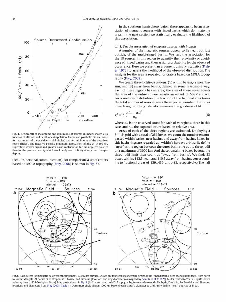
Fig. 4. Reciprocals of maximums and minimums of sources in model shown as afunction of altitude and depth of extrapolation. Linear and parabolic fits are madefor maximums of the positives (solid circles) and for minimums of the negatives(open circles). The negative polarity minimum approaches infinity at J 100 km,suggesting weaker signal and greater noise contribution for the negative polaritythan for the positive polarity which would only reach infinity at very much deeperdepths.

44 D.M. Jurdy, M. Stefanick / Icarus 203 (2009) 38–46

(Schultz, personal communication). For comparison, a set of cratersbased on MOLA topography (Frey, 2008) is shown in Fig. 5b.

Fig. 5. (a) Sources for magnetic field vertical component, Bz at Mars’ surface. Shown are foto south: Mangala, Al Qahira, S. of Hesphaestus Fossae, and Sirenum [locations and ring das heavy lines [USGS Geological Maps]. Map projection as in Fig. 3. (b) Craters based on Mlocations and diameters from Frey (2008, Table 1). Outermost circle shown 1000 km be

In the southern hemisphere region, there appears to be an asso-ciation of magnetic sources with ringed basins which dominate thearea. In the next section we statistically evaluate the likelihood ofthis association.

4.1.1. Test for association of magnetic sources with impactsA number of the magnetic sources appear to lie near, but just

outside, of the multi-ringed basins. We test the association forthe 18 sources in this region to quantify their proximity or avoid-ance of ringed basins and then assign a probability for the observedoccurrence. Here we present an argument using v2 statistics (Fish-er, 1973) to assess the likelihood of the observed distribution. Theanalysis for the area is repeated for craters based on MOLA topog-raphy (Frey, 2008).

We create three fictitious regions: (1) within basins, (2) near ba-sins, and (3) away from basins, defined in some reasonable way.Each of these regions has an area; the sum of these areas equalsthe area of the entire square, nearly an octant of Mars’ surface.For a uniform distribution, the fraction of the fictional area timesthe total number of sources gives the expected number of sourcesin each region. The v2 statistic measures the goodness of fit:

v2 ¼X �nm � nmð Þ2

nmð6Þ

where �nm is the observed count for each of m regions, three in thiscase, and nm, the expected count based on relative area.

Areas of each of the three regions are estimated. Employing a5� � 5� grid with a total of 256 boxes, we count the number encom-passed within basins, near basins, and away from basins. Boxes in-side basin rings are regarded as ‘‘within”; here we arbitrarily define‘‘near” as the region between the outer basin ring out to three radiior a maximum of 3000 km. And those remaining boxes beyond thethree radii limit then count as ‘‘away from basins”. We find: 33boxes within, 112.5 near, and 110.5 away from basins, correspond-ing to fractional areas of .129, .439, and .432, respectively. (The half

ur sets of concentric circles, multi-ringed basins, sites of ancient impacts, from northiameters as mapped by Schultz et al. (1982)]. Faults related to Tharsis-uplift shown

OLA topography, from north to south: Zephyria, Daedalia, SW Daedalia, and Sirenum,yond each crater’s diameter to arbitrarily define ‘‘near”. Sources as in (a).

D.M. Jurdy, M. Stefanick / Icarus 203 (2009) 38–46 45

units come from averaging counts, done twice: once vertically,then horizontally.)

The distribution of magnetic sources is assessed by assigningeach to the one of the three basin regions: within, near, away.The fuzziness of the sources results from, at least in part, thedeconvolution being only approximate. An exact deconvolutionwould require all wavenumbers being used, but we have zeroedout all high wavenumbers to limit noise, as discussed earlier. Theobserved counts: two sources within basins, 14 nearby, and twoaway from basins. However, for a uniform distribution of 18sources with the relative areas determined, we would expect tofind 2.32 sources within the basins, 7.90 near basins and theremaining 7.78 sources in the region defined as away from the ba-sins. For this case v2 can be computed, summing within-, near- andaway from-basin regions:

v2 ¼ ð2� 2:32Þ2

2:32þ ð14� 7:90Þ2

7:90þ ð2� 7:78Þ2

7:78¼ 9:05 ð7Þ

Here, the v2 value is calculated as �9.0. The v2 values for two de-grees of freedom generally lie in the range 0.5–3.0; values greaterthan 6.0 will occur only 5% of the time, a value of 7.8 only 2% ofthe time, and 9.2 only 1% of the time. Therefore the v2 analysis(7) shows the observed distribution of sources and ringed basinsin the southern hemisphere area near 40�S, 180� to be a low-prob-ability occurrence. A slight reinterpretation of source locationsresulting in 13 nearby and three outside would lower the v2 valueto 6.3, having a probability of �5%.

For comparison, we next repeat the statistical analysis for mag-netic sources with another impact scenario. Frey’s (2008) recentglobal assessment of large craters for Mars has been correlatedwith magnetization by Lillis et al. (2008) to establish the durationof Mars’ global magnetic field. Four craters (locations and sizes gi-ven in Table 1, Frey, 2008) fall within 40� of latitude 40�S, 180�W:Zephyria, Daedalia, SW Daedalia, and Sirenum, from north tosouth. (This catalogue positions Sirenum at 67.4�S, 154.7�W,whereas previously a feature at 43.5�S, 166.5�W, about the samesize, was given the same name.) We repeat the v2 analysis. Count-ing 5� boxes for this alternative set of craters we find 51 boxes liewithin the craters, 82 near and the remaining 123 outside, corre-sponding to fractional areas of .199, .320, and .481, respectively.(Here we arbitrarily define ‘‘near” as within 1000 km of each cra-ter’s outer diameter.) For the 18 sources, based on these fractionalareas, 3.6 sources would be expected within craters, 5.8 nearby and8.6 away from craters; however, counting sources we find only onesource lies within a crater, 13 nearby and four away from craters.This corresponds to v2 value of 9.34, an unusual association, occur-ring only � 1% of the time. This statistical analysis in the MartianSouthern Hemisphere strongly suggests that magnetic sources areassociated with ringed basins as the sites of ancient impacts asidentified from geology (Schultz et al., 1982). In addition, re-anal-ysis for an alternative distribution of Mars’ largest craters – onesidentified by Frey (2008) from MOLA topography – with the mag-netic sources in this region, finds this alternative arrangement ofbasins and magnetic sources also unlikely to be random. However,because of the small number of points – 18 magnetic sources here– the results cannot be regarded as conclusive. A more refineddescription of inside-, near- and away-from basins would not re-move the small number problem. Here we have developed andtested a hypothesis: that the strongest magnetic sources are lo-cated adjacent to, but not actually within, very large impacts orringed basins. This can be tested in other regions.

A system of faults extends through the area. Most apparent inthe western region (Scott and Tanaka, 1998), the faults also extendbeyond 180� and die out to the east (Greeley and Guest, 1998). Themodel sources for Bz (Fig. 5) hint at a curious relation to the faults:

often a fault trace separates two locations of strong magnetization.This – if confirmed – might indicate that the uplift of Tharsis andrelated faulting disrupted crust that had already been magnetized.We do not attempt a statistical test for the association, with thelimited number of magnetic sources and faults even more re-stricted than craters. However, the hypothesis merits furtherexamination in other regions where it can be better tested and as-sessed. Possibly, the timing of the faults caused by the uplift ofTharsis could further bracket the duration of the Martian magneticfield.

5. Discussion

All of the ringed basins in the southern hemisphere octant cen-tered on 40�S, 180� have magnetic sources immediately adjacent.The impact process in the presence of an active magnetic fieldcould cause local magnetization. Igneous activity concentratingalong the rings would record the magnetic field at the time of im-pact. If water were present, hydrothermal activity caused by theimpacts could also contribute to magnetization of the ringed ba-sins. Some large craters such as Argyre and Hellas have experi-enced demagnetization, but Mitchell et al. (2007) show Utopia asfeaturing a ring of ‘‘enhanced values” of the crustal magnetic fieldat an altitude of 170 km, B170. So either Utopia demagnetized an al-ready magnetized region, leaving patches, or the sources representmagnetization of Utopia’s inner ring at impact. The latter would,they note, establish the existence of the Martian magnetic fieldat the time of Utopia’s impact. On the basis of crater density Utopiapredates Hellas and Argyre, both lacking internal magnetization(Mitchell et al., 2007).

From numerous studies (e.g. Arkani-Hamed, 2001a; Hood et al.,2005), it appears probable that different regions on Mars weremagnetized relative to different past locations of the magnetic poleand therefore of the spin axis. However, each determination re-quires assumptions, and the resulting paleopole locations scatterconsiderably over the surface. Magnetization of ringed basins attime of impact could offer an independent approach for the deter-mination of magnetic pole locations. If a region were located nearMars’ magnetic north pole at the time of magnetization this wouldaccount for the numerous vertical dipoles causing the correspond-ing excess of positive sources in the southern hemisphere near lat-itude 40�S, longitude 180�. For the path proposed by Schultz andLutz (1988), the pole wanders through this region during the Mid-dle Noachian to the Early Hesperian. In this scenario for Martiantrue polar wander, only the final push about 3 billion years agobrought the pole to its current location (P. Schultz, personal com-munication, 2004).

Confirmation of the cause and timing of magnetization associ-ated with ringed basins requires further examination, particularlythe downward continuation of the field to the surface. Accuratepositioning of magnetic sources at Mars’ surface and possibly be-low, along with the incorporation of MOLA topographic data couldclarify the geometric relation of magnetization to the igneousactivity of the rings. Analysis of an isolated, but similarly-aged ba-sin in another region would be most informative. If the magnetiza-tion resulted from the impacts, this could further constrain theextent of the magnetic field on Mars. The south polar area holdspromise for further modeling.

6. Conclusions

We studied the strongly magnetized region in the southernhemisphere within 40� of the point at 40�S, 180�W, covering nearlyan octant of Mars’ surface. Using a rotated Cartesian coordinatesystem allowed application of ordinary two-dimensional Fourier

46 D.M. Jurdy, M. Stefanick / Icarus 203 (2009) 38–46

analysis for downward continuation. Comparison of downward-continued, mapping level field with aerobraking measurementsmade at 100 km for bins having angular deviation within ±30�yields a 95% correlation for the vertical component, Br . One expla-nation for this agreement would be that the lower-level at�100 km does not contain significant magnetic signal at lowerwavelengths than that measured in the mapping field �400 km.This would have important consequences for the origin and analy-sis of Mars’ magnetic field and requires further analysis. The mag-netic field components were used to model the sources for thefield. A small number of discrete sources, �10–12, more positiveones than negative, can model the field over this large area. How-ever, in a mathematical test of noise, with downward continuationthe negative sources more quickly approach infinity, suggestingweaker inherent signal and a greater contribution of noise. Thismay signify a fundamental difference here between normal and re-versed polarity for Mars’ magnetization.

Models for the field in this southern hemisphere region neitherrequire magnetic stripes with reversals, nor rule out the possibilityeither. Statistical analysis supports the observation that many ofthe strongest magnetic sources appear to lie near to the outer ringsof ancient impacts. The ringed basins, Mangala, Al Qahira, S. ofHesphaestus Fossae, and Sirenum, all have weakly magnetizedinteriors, with magnetic sources situated near their outer rings.These no longer retain the topographic signature of more recentimpact crater and were identified from geological constraints. Sta-tistical analysis was repeated for an alternative set of impact sites,craters identified from their topographic signature. For both ofthese alternatives we test the likelihood of the association by com-paring the observed sources found within and near basins withrandom distribution; the observed distributions were found to bea low-probability occurrence for both of the basin scenarios. Im-pacts in the presence of a magnetic field – and perhaps water –may be responsible for the observed magnetization around ringedbasins. In this southern hemisphere region there are only a fewlarge impacts and about a dozen magnetic sources. Therefore, thehypothesis that the strongest magnetic sources are positionedadjacent to, but not actually within, very large impacts or ringedbasins needs to be tested elsewhere. If a geometric relation be-tween the magnetization and impact rings could be established,this might offer an independent approach for determining Martianpaleomagnetic poles. If confirmed, then the magnetization may becontemporaneous with the impacts; this would provide an addi-tional constraint on the duration of Mars’ magnetic field.

Acknowledgments

The MGS mapping dataset, binned by latitudes and longitudes,was the basis of our study. This dataset was generously made avail-able to the scientific community by Connerney and coauthors; wethank Jack Connerney for discussions on noise and downward con-tinuation. We are grateful to Pete Schultz for sharing his insightson impacts and for his continued encouragement. Finally, we thankEditor Jim Bell for his forbearance. We are grateful for funding fromMars Data Analysis Program, Grant #NAG5-12157 that supportedthis research.

References

Acuna, M.H., and 13 colleagues, 1999. Global distribution of crustal magnetizationdiscovered by the Mars Global Surveyor MAG/ER experiment. Science 284, 790–793.

Arkani-Hamed, J., 2001a. Paleomagnetic pole positions and pole reversals of Mars.Geophys. Res. Lett. 17, 3409–3412.

Arkani-Hamed, J., 2001b. A 50-degree spherical harmonic model of the magneticfield of Mars. J. Geophys. Res. 106, 23197–23208.

Cain, J.C., Ferguson, B.B., Mozzoni, D., 2003. An n = 90 internal potential function ofthe martian crustal magnetic field. J. Geophys. Res., 108. doi:10.1029/2000JE001487.

Carslaw, H.S., 1930. Introduction to the Theory of Fourier Series and Integrals.Dover, New York.

Claerbout, J.F., 1976. Fundamentals of Geophysical Data Processing. McGraw-Hill,New York. 274pp.

Connerney, J.E.P., Acuna, M.H., Wasilewski, P.J., Ness, N.F., Reme, H., Mazelle, C.,Vignes, D., Lin, R.P., Mitchell, D.L., Cloutier, P.A., 1999. Magnetic lineations in theancient crust of Mars. Science 284, 794–798.

Connerney, J.E.P., Acuna, M.H., Wasilewski, P.J., Kletetschka, G., Ness, N.F., Reme, H.,Lin, R.P., Mitchell, D.L., 2001. The global magnetic field of Mars and implicationsfor crustal evolution. Geophys. Res. Lett. 28, 4015–4018.

Connerney, J.E.P., Acuna, M.H., Ness, N.F., Mitchell, D.L., Lin, R.P., Reme, H., 2005.Tectonic implications of Mars crustal magnetism. Proc. Natl. Acad. Sci. USA 102,14970–14975.

Dahlquist, G., Bjorck, A., 1997. Numerical Methods. Prentice-Hall, Englewood Cliffs,NJ. 573pp.

Espley, J.R., Connerney, J.E.P., Jurdy, D.M., Acuna, M.H., 2007. Downwardcontinuation of the martian magnetic field. Lunar Planet. Sci. XXXVIII (abstract).

Fisher, R.A., 1973. Statistical Methods for Research Workers. Hafner, New York.362pp.

Frey, H.V., 2008. Ages of very large impact basins on Mars: Implications for the lateheavy bombardment in the inner Solar System. Geophys. Res. Lett., 35.doi:10.1029/2008GL033515.

Greeley, R., Guest, J.E., 1998. Geologic map of the eastern equatorial region of Mars.USGS, Geological Investigations Series Map I, I-1802-B.

Hood, L.L., Young, C.N., Richmond, N.C., Harrison, K.P., 2005. Modeling of majormartian magnetic anomalies: Further evidence for polar reorientations duringthe Noachian. Icarus 177, 144–173.

Jurdy, D.M., Stefanick, M., 2003. Mars magnetic data: The impact of noise on thevertical extrapolation of fields and methods of suppression (abstract). LunarPlanet. Sci. XXXIII.

Jurdy, D.M., Stefanick, M., 2004. Vertical extrapolation of Mars magnetic potentials.J. Geophys. Res., doi:10.1029/2004JE002277.

Kanasewich, E.R., 1981. Time Sequence Analysis in Geophysics. University of AlbertaPress, Alberta, Canada. 480pp.

Klein, F., 1925. Arithmetic, Algebra, Analysis, third ed., Translated by E.R. Hedrickand C.A. Noble. Dover, New York.

Lillis, R.J., Frey, H.V., Manga, M., 2008. Rapid decrease in martian crustalmagnetization in the Noachian era: Implications for the dynamo and climateof early Mars. Geophys. Res. Lett. 35. doi:10.1029/2008GL034338.

Mitchell, D.L., Lillis, R., Lin, P., Connerney, J., Acuna, M., 2007. A global map of Mars’crustal magnetic field based on electron reflectometry. J. Geophys. Res. 112 (E1),E01002. doi:10.1029/2005JE002564.

Morgan, J., Warner, M., 1999. Chicxulub: The third dimension of a multi-ring impactbasin. Geology 27, 407–410.

Nagy, A.F., and 14 colleagues, 2004. The plasma environment of Mars. Space Sci.Rev. 111, 33–114.

Nimmo, F., Gilmore, M.S., 2001. Comments on the depth of magnetized crust onMars from impact craters. J. Geophys. Res. 106, 11315–11323.

Parnell, J., Osinski, G.R., Lee, P., Green, P.F., Baron, M.J., 2005. Thermal alteration oforganic material in an impact crater and the duration of post-impact heating.Geology 33, 373–376.

Press, W.H., Teukolsky, S.A., Vetterling, W.T., Flannery, B.P., 1992. Numerical Recipesin FORTRAN. Cambridge University Press, New York. 818pp.

Rochette, P., Fillion, G., Ballou, R., Brunet, F., Ouladdiaf, B., Hood, L., 2003. Highpressure magnetic transition in pyrrhotite and impact demagnetization onMars. Geophys. Res. Lett. 30 (13), 1683. doi:10.1029/2003GL017359.

Schultz, P.H., Lutz, A.B., 1988. Polar wandering on Mars. Icarus 73, 91–141.Schultz, P.H., Schultz, R.A., Rogers, J., 1982. The structure and evolution of ancient

impact craters on Mars. J. Geophys. Res. 87, 9803–9820.Scott, D.H., Tanaka, K.L., 1998. Geologic map of the western equatorial region of

Mars. USGS, Geological Investigations Series.Sleep, N.H., 1994. Martian plate tectonics. J. Geophys. Res. 99, 5639–5655.Tanaka, K.L., Scott, D.H., 1998. Geologic map of the polar regions of Mars. USGS,

Geological Investigations Series Map I, I-1802-C.