Icarus 189 (2007) 325–343www.elsevier.com/locate/icarus

Dust storms originating in the northern hemisphere during the third mappingyear of Mars Global Surveyor

Huiqun Wang

Atomic and Molecular Physics Division, Smithsonian Astrophysical Observatory, 60 Garden St., Cambridge, MA 02138, USA

Received 28 April 2006; revised 24 December 2006

Available online 24 February 2007

Abstract

Data from the third Mars Global Surveyor (MGS) mapping year (MY 26, 2003–2005) are used to investigate dust storms originating in thenorthern hemisphere. Flushing dust storms, which originate as frontal dust storms at the northern polar vortex edge and propagate southwardthrough topographic channels, are observed immediately before and after a quiescent period that occurs around the northern winter solstice(240◦ < Ls < 300◦). Both the pre- and post-solstice active periods can be further divided into two sub-periods. The most vigorous of theseflushing storms occurred during Ls 210–220◦ and Ls 310–320◦. The lifted dust crossed the equator and accumulated in the southern hemisphere.These major dust storms enhanced the Hadley circulation and suppressed the lower-level baroclinic eddies in the northern mid and high latitudes.The 2–3 sol wave number m = 3 traveling waves show the best correlation with flushing dust storms and can combine with other wave modes toproduce storm tracks and fronts within individual sub-periods.© 2007 Elsevier Inc. All rights reserved.

Keywords: Mars, atmosphere

1. Introduction

Mars Global Surveyor (MGS) has been continuously mon-itoring global martian meteorology for more than three Marsyears. The data returned by MGS have been used to study thedistribution of dust, clouds, and water vapor in great detail (e.g.,Cantor et al., 2001; Wang and Ingersoll, 2002; Smith, 2004;Wang et al., 2005). Among the many findings of MGS arethe “flushing dust storms” which originate at the north po-lar vortex edge as frontal dust storms and propagate south-ward through confined longitude channels (Cantor et al., 2001;Wang et al., 2003). The most intense flushing storms can trans-port dust across the equator to the southern hemisphere. Flush-ing events initially keep the curved or linear frontal structuresindicative of baroclinic eddies; however, once the dust stormsmove south, they usually exhibit irregular patchy shapes andcan be enhanced by additional dust lifting along the way. Us-ing the data obtained by MGS from 1999 to 2003, Wang etal. (2005) showed that flushing dust storms are concentrated

E-mail address: hwang@cfa.harvard.edu.

0019-1035/$ – see front matter © 2007 Elsevier Inc. All rights reserved.doi:10.1016/j.icarus.2007.01.014

in Acidalia, Arcadia, and Utopia, are active during the peri-ods away from the northern winter solstice, and correlate es-pecially well with the 2–3 sol wavenumber m = 3 eastwardtraveling waves in the lowest atmospheric scale height. Further-more, Wang et al. (2003) suggested that consecutive flushingdust storms could lead to major dust storms of global impact.

The development of flushing storms involves interactionsamong baroclinic eddies, thermal tides, and the Hadley circu-lation (Wang et al., 2003). Together with the suggestion thatmajor dust storms could suppress subsequent development ofbaroclinic eddies (Leovy et al., 1985; Wang et al., 2005), thisled Wang et al. (2005) to hypothesize that the timing of ma-jor dust storms could affect the seasonal distribution of flushingdust storms: a major dust storm in the early fall or mid wintercould be followed first by a period with no frontal dust storms,and, subsequently, by a period with active flushing dust storms.An overview of past work can be found in Wang et al. (2005),and is not repeated here.

To investigate the interannual variability and test the hypoth-esis in Wang et al. (2005), this paper presents the distributionof dust storms originating in the northern hemisphere during thethird MGS mapping year (MY 26, 2003–2005). The dust storms

326 H. Wang / Icarus 189 (2007) 325–343

are either flushing dust storms or are related to flushing duststorms. The histories of two dust storm sequences initiated byflushing dust storms are described in detail. These dust stormspropagated from the northern to the southern hemisphere andresulted in dust accumulation in the southern hemisphere. Theimpacts of these dust storms on the atmospheric thermal struc-tures and transient eddy activities are also investigated.

2. Data

This study mainly uses the Mars Daily Global Maps(MDGM) derived from the MGS Mars Observer Camera(MOC) global map swaths and the vertical temperature profilesand dust opacities derived from the MGS Thermal EmissionSpectrometer (TES) spectra. MDGM are composed using themethod described in Wang and Ingersoll (2002), and are an-alyzed using the same method as that in Wang et al. (2005).Version 2 MGS TES temperatures and opacities are extractedusing the “vanilla” software from the released archives at thePlanetary Data System (PDS). The TES data selection criteriainclude “atm_pt_rating = 0, atm_opacity_rating = 0 (the re-trieval is good), and emission angle <5◦”. Some MGS MOCwide angle images and MGS Radio Science temperature pro-files are presented as supplementary materials in this paper aswell.

3. Dust storm distribution

3.1. MOC observations

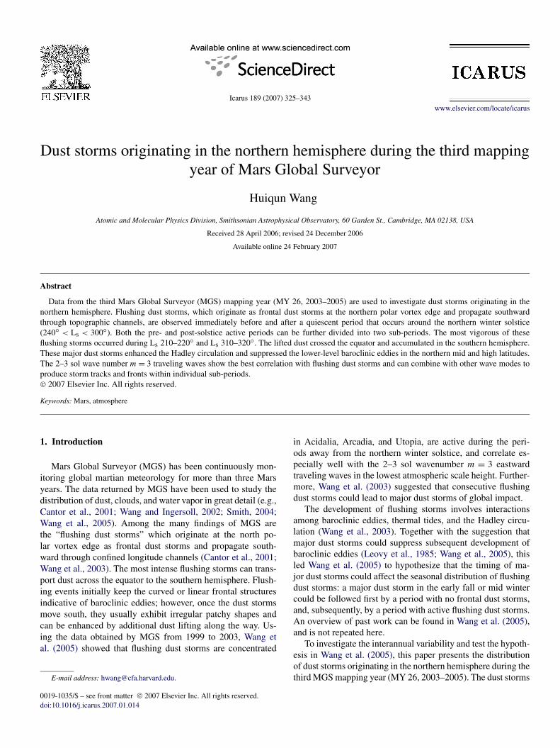
Fig. 1 shows the Ls–latitude distribution of dust storms thatoccur within 60◦ S–60◦ N, originate in the northern hemi-sphere, and show history or morphology indicative of south-ward motion. The method for selecting dust storms is the sameas that in Wang et al. (2005). Figs. 1a and 1b show the updatedversion for the first (MY 24, 1999–2001) and second (MY 25,2001–2003) MGS mapping years, and Fig. 1c shows the newlycompleted results for the third (MY 26, 2003–2005) MGS map-ping year. All flushing dust storms (Wang et al., 2003, 2005) aretracked: diamonds with plus signs indicate new flushing duststorms, hollow diamonds indicate both dust storms that resultfrom flushing dust storms and a few ambiguous dust storms.Dust storms that last multiple days or dust storms that merge areconnected with lines. There are 142, 108, and 162 new flushingdust storms in Figs. 1a, 1b, and 1c, respectively. Fig. 1 does notinclude dust storms that are clearly associated with topographyor albedo, or dust storms that originate in the southern hemi-sphere. However, with the exception of the 2001 (MY 25, Ls ∼182◦) global dust storm which shows explosive developmentfrom the southern to the northern hemisphere (Smith, 2004;Strausberg et al., 2005), Fig. 1 provides a good summary ofthe main dust storm activities within 60◦ S–60◦ N.

A detailed study of the first and second MGS mapping years(MY 24 and MY 25) can be found in Wang et al. (2005), this pa-per concentrates on the third year (MY 26). In agreement withthe previous two years, flushing dust storms in MY 26 are con-fined to two separate seasonal windows: the pre-solstice and

post-solstice periods. During the “gap” period (Ls 240◦–300◦)between the two seasonal windows, streaks are present at theedge of the north polar hood and the atmosphere appears dusty,but no frontal dust storms are observed. Detailed examinationof Fig. 1c shows that within each seasonal window, there aretwo active sub-periods of flushing dust storms with a short gapbetween them. Although each active sub-period contains onlya few flushing dust storms, they both include one long-lasting(more than ∼ one week) dust storm sequence. The pre-solsticewindow contains the short gap of Ls ∼ 220◦–230◦ and the post-solstice window contains the short gap of Ls ∼ 320◦–330◦.There are 8, 3, 10, and 12 distinct flushing events duringLs 210◦–220◦, Ls 230◦–240◦, Ls 310◦–320◦, and Ls 330◦–340◦, respectively. Short gaps are not apparent in MY 24 andMY 25 (Figs. 1a and 1b). Later sections will show that the flush-ing dust storms before Ls ∼ 220◦ and those before Ls ∼ 320◦have a significant impact on the global atmospheric tempera-ture structures during the short gaps, and that the effects of theperturbations subside before the next active flushing sub-periodbegins. The flushing dust storms in the post-solstice periods ofMY 24 and MY 25 did not have appreciable effects on thelarge-scale temperature structures, which might be the reasonfor the lack of short gaps during these periods. Although theflushing storms in the pre-solstice period of MY 24 led to the1999 planet-encircling dust storm which significantly perturbedthe atmospheric temperatures (Liu et al., 2003; Smith (2004);Wang et al., 2003, 2005), the long northern winter solstice gaphad begun by the end of this storm (Ls ∼ 240◦), preventing asecond period of flushing dust storms before the solstice. Hadthe 1999 planet-encircling storm finished earlier, there couldhave been an additional episode of flushing dust storms in thenorthern fall of MY 24.

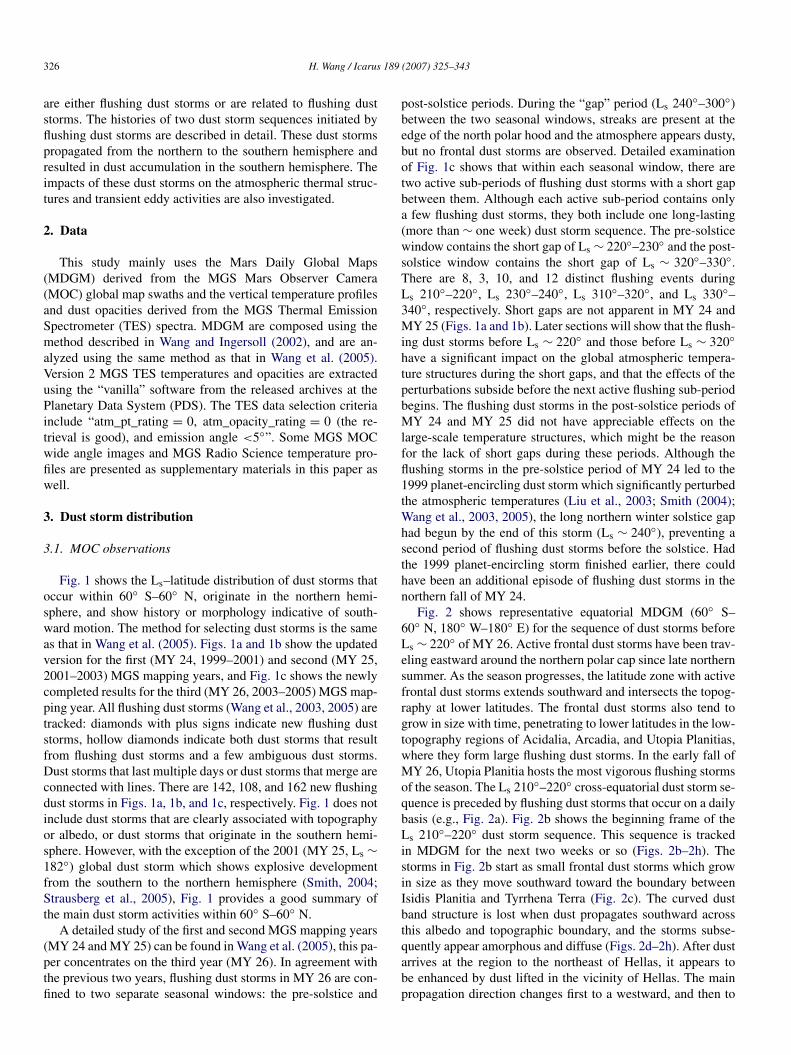
Fig. 2 shows representative equatorial MDGM (60◦ S–60◦ N, 180◦ W–180◦ E) for the sequence of dust storms beforeLs ∼ 220◦ of MY 26. Active frontal dust storms have been trav-eling eastward around the northern polar cap since late northernsummer. As the season progresses, the latitude zone with activefrontal dust storms extends southward and intersects the topog-raphy at lower latitudes. The frontal dust storms also tend togrow in size with time, penetrating to lower latitudes in the low-topography regions of Acidalia, Arcadia, and Utopia Planitias,where they form large flushing dust storms. In the early fall ofMY 26, Utopia Planitia hosts the most vigorous flushing stormsof the season. The Ls 210◦–220◦ cross-equatorial dust storm se-quence is preceded by flushing dust storms that occur on a dailybasis (e.g., Fig. 2a). Fig. 2b shows the beginning frame of theLs 210◦–220◦ dust storm sequence. This sequence is trackedin MDGM for the next two weeks or so (Figs. 2b–2h). Thestorms in Fig. 2b start as small frontal dust storms which growin size as they move southward toward the boundary betweenIsidis Planitia and Tyrrhena Terra (Fig. 2c). The curved dustband structure is lost when dust propagates southward acrossthis albedo and topographic boundary, and the storms subse-quently appear amorphous and diffuse (Figs. 2d–2h). After dustarrives at the region to the northeast of Hellas, it appears tobe enhanced by dust lifted in the vicinity of Hellas. The mainpropagation direction changes first to a westward, and then to

Dust storms in the third MGS mapping year 327

Fig. 1. Ls–latitude distribution of dust storms originating in the northern hemisphere. The three panels show results for MGS mapping years 1 (MY 24, 1999–2001),2 (MY 25, 2001–2003), and 3 (MY 26, 2003–2005), respectively. Diamonds with plus signs indicate new frontal dust storms (frontal dust storms suggestive ofsouthward motion). Hollow diamonds are either dust storms that can be traced to previous storms or questionable flushing dust storms. Dust storms that last multipledays or dust storms that merge are connected with lines. The regions in shadows indicate periods with no images.

a southward direction (Figs. 2e–2h). Dust temporarily accumu-lates in Noachis Terra (west of Hellas, Fig. 2h) and dissipateswithin about four days. During the course of this sequence, sev-eral flushing dust storms are observed in Acidalia and Arcadia(e.g., Fig. 2f), although these storms do not cross the equator.After the sequence finishes at Ls ∼ 219◦, there is a ∼20-dayhiatus when the northern mid and high latitudes are dominatedby streaks without any flushing dust storms. The hiatus is fol-lowed by a brief period (∼one week, Ls 230◦–235◦) of activeflushing dust storms in the Acidalia channel. The first flushing

dust storm for this sub-period can be found in Fig. 5i of Wanget al. (2005). It travels southward across the equator and dissi-pates in the region to the southeast of Valles Marineris’ EOSChasma.

The post-solstice period starts around Ls ∼ 310◦ when vig-orous frontal dust storms return at northern mid and high lat-itudes. Fig. 3 shows representative MDGM for the sequenceof dust storms that can be tracked to the southern hemisphere.The first day (Fig. 3a, Ls ∼ 314◦) of the sequence is precededby about a week of frontal dust storms, some of which are

328 H. Wang / Icarus 189 (2007) 325–343

Fig. 2. Representative MDGM (60◦ S–60◦ N, 180◦ W–180◦ E, simple cylindrical projection) illustrating the development of the Ls 210◦–220◦ dust storm sequence.The Ls for each panel is (a) 206.5◦ , (b) 211.4◦ , (c) 212.0◦ , (d) 212.7◦ , (e) 213.3◦ , (f) 213.9◦ , (g) 214.5◦ , (h) 215.7◦ . The dust storms described in the text areindicated by arrows.

Dust storms in the third MGS mapping year 329

Fig. 2. (continued)

330 H. Wang / Icarus 189 (2007) 325–343

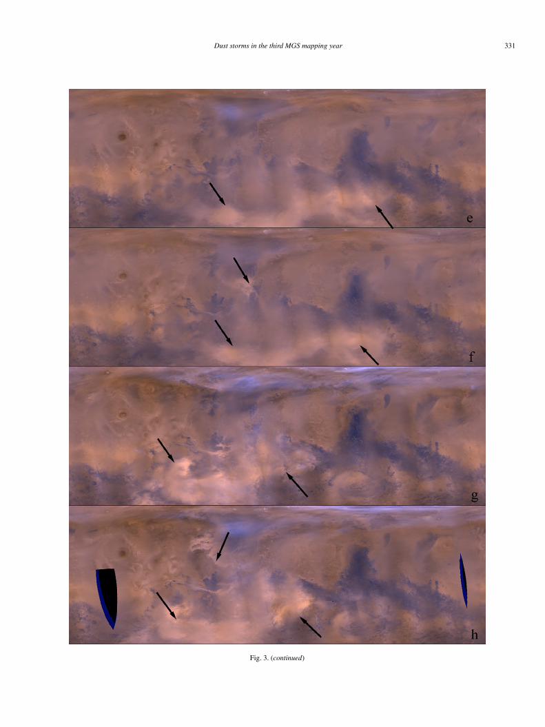
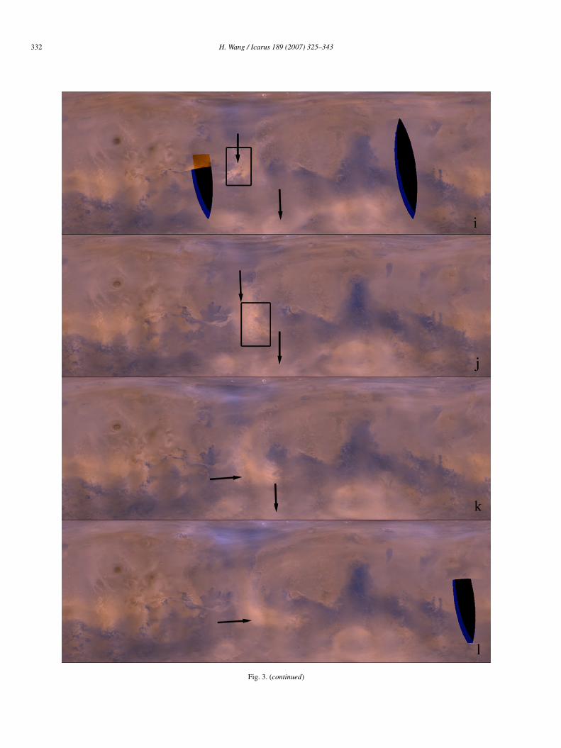
Fig. 3. Representative MDGM (60◦ S–60◦ N, 180◦ W–180◦ E, simple cylindrical projection) illustrating the development of the Ls 310◦–320◦ dust storm sequence.The Ls for each panel is (a) 314.1◦ , (b) 314.7◦ , (c) 315.3◦ , (d) 315.9◦ , (e) 316.4◦ , (f) 317.0◦ , (g) 319.8◦ , (h) 320.4◦ , (i) 320.9◦ , (j) 321.4◦ , (k) 322.1◦ , (l) 322.6◦ .The dust storms described in the text are indicated by arrows. The rectangles in (i) and (j) indicate the regions displayed in Fig. 4.

Dust storms in the third MGS mapping year 331

Fig. 3. (continued)

332 H. Wang / Icarus 189 (2007) 325–343

Fig. 3. (continued)

Dust storms in the third MGS mapping year 333

Fig. 4. MGS MOC wide angle image (a) r1202744, Ls = 321.06, 1046.45 m/pixel and (b) r1202883, Ls = 321.61, 1036.17 m/pixel. The storm in (a) is the sameas that near Valles Marineris in Fig. 3i, and the storm in (b) is the same as that near Valles Marineris in Fig. 3j. Both images are in the same simple cylindricalprojection as the MDGM. The area in (a) covers 15◦ S–10◦ N, 322◦ E–334◦ E. The area in (b) covers 24◦ S–0◦ , 338◦ E–350◦ E.

flushing dust storms (frontal dust storms that show southwardmotion). On the first day (Fig. 3a), a flushing dust storm extendsits dust band from the polar hood to southern Acidalia Plani-tia and another dust storm, which may be either dust flushedsouthward by a previous flushing storm or a local storm, cov-ers Chryse. Dust subsequently travels in a general southwarddirection for the next three days and reaches latitudes southof 60◦ S (Figs. 3b–3d), where it appears to be enhanced bydust lifting near Argyre and develops both to the west and tothe east (Fig. 3e). Additional flushing dust storms in Acidalia–Chryse also make contributions to the dust load in the southernhemisphere (Fig. 3f). The main body of dust arranges into asoutheast–northwest elongated belt that straddles Argyre andHellas (Figs. 3g–3i). The dust belt gradually merges into thebackground afterwards (Figs. 3j–3l). In the meantime, somedust from south of Argyre goes to the polar region (Ls ∼ 317◦),and encircles the south polar cap from the west to the east (notshown). The polar dust from this event settles down after abouta week. Of all the major dust storms observed by MGS, onlythe 2001 global dust storm (Strausberg et al., 2005) and thisMY 26 Ls 310◦–320◦ event exported dust to the south polarregion. These two major dust storms also have the first and sec-ond longest duration of dusty atmosphere in the southern hemi-sphere. Previous data and numerical simulations show that thepresence of substantial amounts of dust in the southern hemi-sphere during southern spring and summer will significantlyaffect the global atmospheric structure and circulation (Smith,2004; Wilson, 1997; Wilson and Richardson, 2000). The im-

pacts of the MY 26 post-solstice dust storms will be presentedin later sections.

After the dust belt forms in the southern mid and high lat-itudes, a second sequence of southward-moving dust stormsforms near Chryse at Ls ∼ 320◦ (Fig. 3h). Whether the firststorm of this second sequence is related to a flushing dust stormis questionable. Nevertheless, dust travels southward across theequator and temporarily accumulates (for about a week) in theregion to the south and east of Valles Marineris (Figs. 3i–3l).This sequence greatly boosts the amount of dust in the southernhemisphere while dust from the previous sequence is dissipat-ing. The MOC WA camera captured 1 km/pixel views of thestorms (Fig. 4) in addition to the 7.5 km/pixel global mapswaths. Figs. 4a and 4b show the same dust storms as those nearValles Marineris in Figs. 3i and 3j, respectively. A stripe patternin the northwest–southeast direction is observed in the middlepart (just north of Valles Marineris) of Fig. 4a. The directionof the stripes appears to be perpendicular to the direction ofdust storm motion (indicated by the arrow). The part south ofthe stripes appears amorphous, perhaps due to the interactionwith the complex terrain of Valles Marineris. The dust stormin Fig. 4b exhibits a fluffy, blotchy texture common to maturedust storms. It has mostly passed Valles Marineris and is travel-ing in a general southward direction in Margaritifer Sinus (theupper part) and in an eastward direction south of it (the lowerpart). Curved dark lines or lobes perpendicular to the propa-gation directions (indicated by the arrows) are discernable inplaces despite the generally turbulent appearance of the duststorm.

334 H. Wang / Icarus 189 (2007) 325–343

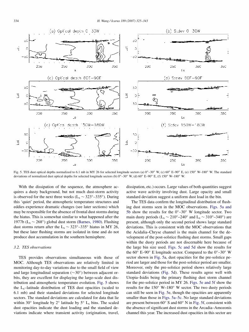
Fig. 5. TES dust optical depths normalized to 6.1 mb in MY 26 for selected longitude sectors (a) 0◦–30◦ W, (c) 60◦ E–90◦ E, (e) 150◦ W–180◦ W. The standarddeviations of normalized dust optical depths for selected longitude sectors (b) 0◦–30◦ W, (d) 60◦ E–90◦ E, (f) 150◦ W–180◦ W.

With the dissipation of the sequence, the atmosphere ac-quires a dusty background, but not much dust-storm activityis observed for the next three weeks (Ls ∼ 323◦–335◦). Duringthis ‘quiet’ period, the atmospheric temperature structures andeddies experience dramatic changes (see later sections) whichmay be responsible for the absence of frontal dust storms duringthe hiatus. This is somewhat similar to what happened after the1977b (Ls ∼ 268◦) global dust storm (Barnes, 1980). Flushingdust storms return after the Ls ∼ 323◦–335◦ hiatus in MY 26,but these later flushing storms are isolated in time and do notproduce dust accumulation in the southern hemisphere.

3.2. TES observations

TES provides observations simultaneous with those ofMOC. Although TES observations are relatively limited inmonitoring day-to-day variations due to the small field of viewand large longitudinal separation (∼30◦) between adjacent or-bits, they are excellent for displaying the large-scale dust dis-tribution and atmospheric temperature evolution. Fig. 5 showsthe Ls–latitude distribution of TES dust opacities (scaled to6.1 mb) and their standard deviations for selected longitudesectors. The standard deviations are calculated for data that liewithin 30◦ longitude by 2◦ latitude by 5◦ Ls bins. The scaleddust opacities indicate the dust loading and the standard de-viations indicate where transient activity (origination, travel,

dissipation, etc.) occurs. Large values of both quantities suggestactive wave activity involving dust. Large opacity and smallstandard deviation suggest a uniform dust load in the bin.

The TES data confirm the longitudinal distribution of flush-ing dust storms seen in the MOC observations. Figs. 5a and5b show the results for the 0◦–30◦ W longitude sector. Twomain dusty periods (Ls ∼ 210◦–240◦ and Ls ∼ 310◦–340◦) arepresent, although only the second period shows large standarddeviations. This is consistent with the MOC observations thatthe Acidalia–Chryse channel is the main channel for the de-velopment of the post-solstice flushing dust storms. Small gapswithin the dusty periods are not discernable here because ofthe large bin size used. Figs. 5c and 5d show the results forthe 60◦ E–90◦ E longitude sector. Compared to the 0◦–30◦ Wsector shown in Fig. 5a, dust opacities for the pre-solstice pe-riod are larger and those for the post-solstice period are smaller.Moreover, only the pre-solstice period shows relatively largestandard deviations (Fig. 5d). These results agree well withUtopia–Isidis being the primary flushing dust storm channelfor the pre-solstice period in MY 26. Figs. 5e and 5f show theresults for the 150◦ W–180◦ W sector. The two dusty periodscan still be seen in Fig. 5e, though the opacities are apparentlysmaller than those in Figs. 5a–5c. No large standard deviationsare present between 60◦ S and 60◦ N in Fig. 5f, consistent withthe absence of significant dust storms in the Arcadia–Amozonischannel this year. The increased dust opacities in this sector are

Dust storms in the third MGS mapping year 335

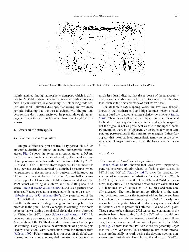
Fig. 6. Zonal mean TES atmospheric temperatures at 50.1 Pa (∼25 km) as a function of latitude and Ls for MY 26.

mainly attained through atmospheric transport, which is diffi-cult for MDGM to show because the transported dust does nothave a clear structure or a boundary. All other longitude sec-tors also exhibit elevated dust opacities during the two dustyperiods, indicating that the dust associated with the pre- andpost-solstice dust storms encircled the planet, although the av-erage dust opacities are much smaller than those for global duststorms.

4. Effects on the atmosphere

4.1. The zonal mean temperature

The pre-solstice and post-solstice dusty periods in MY 26produce a significant impact on global atmospheric temper-atures. Fig. 6 shows the zonal-mean temperatures at 0.5 mb(∼25 km) as a function of latitude and Ls. The rapid increaseof temperatures coincides with the initiation of the Ls 210◦–220◦ and Ls 310◦–320◦ dust storm sequences. Furthermore, thedusty periods are characterized by dumbbell structures wheretemperatures at the northern and southern mid latitudes arehigher than those at the low latitudes. A dumbbell structurein the upper level temperature field is also associated with the1999 planet-encircling dust storm and the 2001 global duststorm (Smith et al., 2002; Smith, 2004), and is a signature of anenhanced Hadley circulation associated with major dust storms(Haberle et al., 1993; Wilson, 1997). The perturbation of theLs 310◦–320◦ dust storms is especially impressive consideringthat the isotherms delineating the edge of northern polar vortexprotrude to the pole. The only other polar warming in the northpolar region was during the solstitial global dust storm observedby Viking (the 1977b storm) (Jakosky and Martin, 1987). Nopolar warming was associated with the 2001 global dust storm.A simulation of the 1977b global dust storm shows that the po-lar warming is largely due to the development of a pole-to-poleHadley circulation, with contribution from the thermal tides(Wilson, 1997). Polar warming does not occur in all global duststorms, but can occur in non-global dust storms which involve

much less dust indicating that the response of the atmosphericcirculation depends sensitively on factors other than the dustload, such as the time and mode of dust storm onset.

For all three MGS mapping years, the low-level temper-atures in the southern mid and high latitudes reach a maxi-mum around the southern summer solstice (not shown) (Smith,2004). There is an indication that higher temperatures relatedto the dust storm sequences occur in the southern hemisphere,but the signal is not as prominent as that in the upper levels.Furthermore, there is no apparent evidence of low-level tem-perature perturbations in the northern polar region. It thereforeappears that the upper level atmospheric temperatures are betterindicators of major dust storms than the lower level tempera-tures.

4.2. Eddies

4.2.1. Standard deviations of temperaturesWang et al. (2005) showed that lower level temperature

perturbations were closely related to flushing dust storms inMY 24 and MY 25. Figs. 7a and 7b show the standard de-viations of temperature perturbations for MY 26 at 4.75 mb(∼2.5 km) derived from the TES 2PM and 2AM tempera-tures, respectively. The standard deviations are calculated for30◦ longitude by 2◦ latitude by 10◦ Ls bins and then zon-ally averaged. The most important contributions to the stan-dard deviations are from the transient eddies. In the southernhemisphere, the maximum during Ls 310◦–320◦ clearly cor-responds to the post-solstice dust storm sequence describedin Section 3 and is present in both the 2PM and 2AM plots.There appear to be enhanced 2PM temperature variations in thesouthern hemisphere during Ls 210◦–220◦ which would cor-respond to the pre-solstice cross-equatorial dust storms. How-ever, these enhanced variations are not present in the 2AMplot; Fig. 7 shows that the 2PM variations are generally largerthan the 2AM variations. This perhaps relates to the mecha-nisms preferentially at work during the daytime such as con-vection and dust devils. Considering that the Ls 210◦–220◦

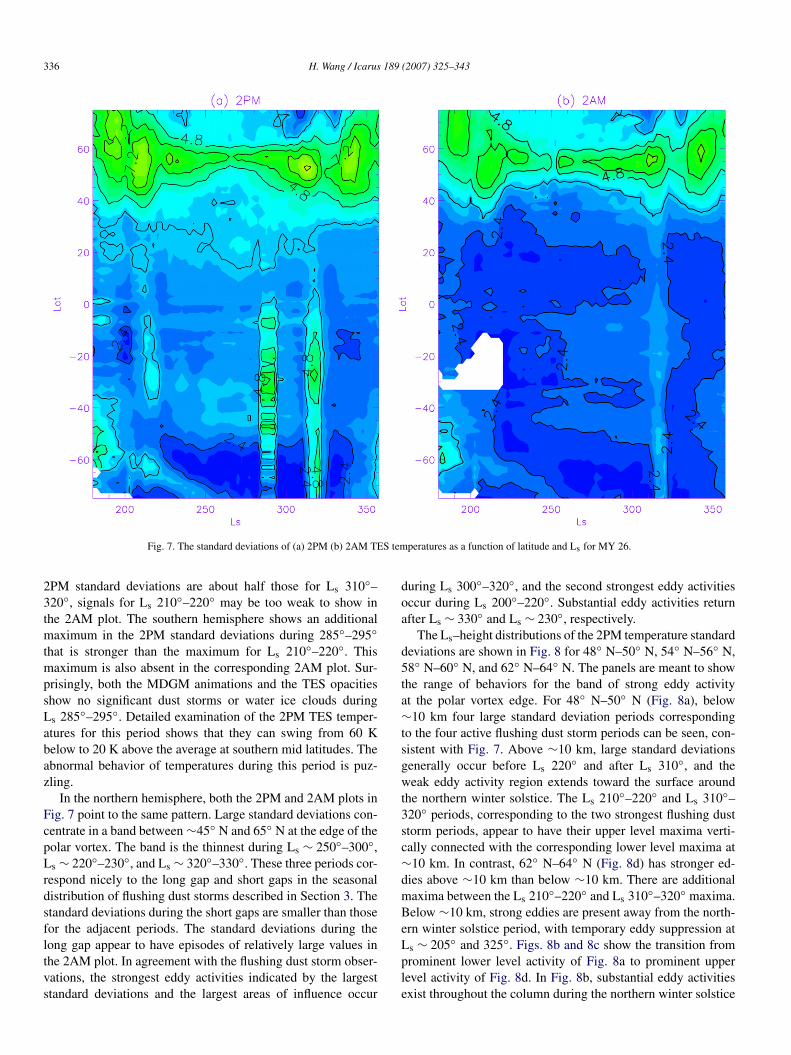
336 H. Wang / Icarus 189 (2007) 325–343

Fig. 7. The standard deviations of (a) 2PM (b) 2AM TES temperatures as a function of latitude and Ls for MY 26.

2PM standard deviations are about half those for Ls 310◦–320◦, signals for Ls 210◦–220◦ may be too weak to show inthe 2AM plot. The southern hemisphere shows an additionalmaximum in the 2PM standard deviations during 285◦–295◦that is stronger than the maximum for Ls 210◦–220◦. Thismaximum is also absent in the corresponding 2AM plot. Sur-prisingly, both the MDGM animations and the TES opacitiesshow no significant dust storms or water ice clouds duringLs 285◦–295◦. Detailed examination of the 2PM TES temper-atures for this period shows that they can swing from 60 Kbelow to 20 K above the average at southern mid latitudes. Theabnormal behavior of temperatures during this period is puz-zling.

In the northern hemisphere, both the 2PM and 2AM plots inFig. 7 point to the same pattern. Large standard deviations con-centrate in a band between ∼45◦ N and 65◦ N at the edge of thepolar vortex. The band is the thinnest during Ls ∼ 250◦–300◦,Ls ∼ 220◦–230◦, and Ls ∼ 320◦–330◦. These three periods cor-respond nicely to the long gap and short gaps in the seasonaldistribution of flushing dust storms described in Section 3. Thestandard deviations during the short gaps are smaller than thosefor the adjacent periods. The standard deviations during thelong gap appear to have episodes of relatively large values inthe 2AM plot. In agreement with the flushing dust storm obser-vations, the strongest eddy activities indicated by the largeststandard deviations and the largest areas of influence occur

during Ls 300◦–320◦, and the second strongest eddy activitiesoccur during Ls 200◦–220◦. Substantial eddy activities returnafter Ls ∼ 330◦ and Ls ∼ 230◦, respectively.

The Ls–height distributions of the 2PM temperature standarddeviations are shown in Fig. 8 for 48◦ N–50◦ N, 54◦ N–56◦ N,58◦ N–60◦ N, and 62◦ N–64◦ N. The panels are meant to showthe range of behaviors for the band of strong eddy activityat the polar vortex edge. For 48◦ N–50◦ N (Fig. 8a), below∼10 km four large standard deviation periods correspondingto the four active flushing dust storm periods can be seen, con-sistent with Fig. 7. Above ∼10 km, large standard deviationsgenerally occur before Ls 220◦ and after Ls 310◦, and theweak eddy activity region extends toward the surface aroundthe northern winter solstice. The Ls 210◦–220◦ and Ls 310◦–320◦ periods, corresponding to the two strongest flushing duststorm periods, appear to have their upper level maxima verti-cally connected with the corresponding lower level maxima at∼10 km. In contrast, 62◦ N–64◦ N (Fig. 8d) has stronger ed-dies above ∼10 km than below ∼10 km. There are additionalmaxima between the Ls 210◦–220◦ and Ls 310◦–320◦ maxima.Below ∼10 km, strong eddies are present away from the north-ern winter solstice period, with temporary eddy suppression atLs ∼ 205◦ and 325◦. Figs. 8b and 8c show the transition fromprominent lower level activity of Fig. 8a to prominent upperlevel activity of Fig. 8d. In Fig. 8b, substantial eddy activitiesexist throughout the column during the northern winter solstice

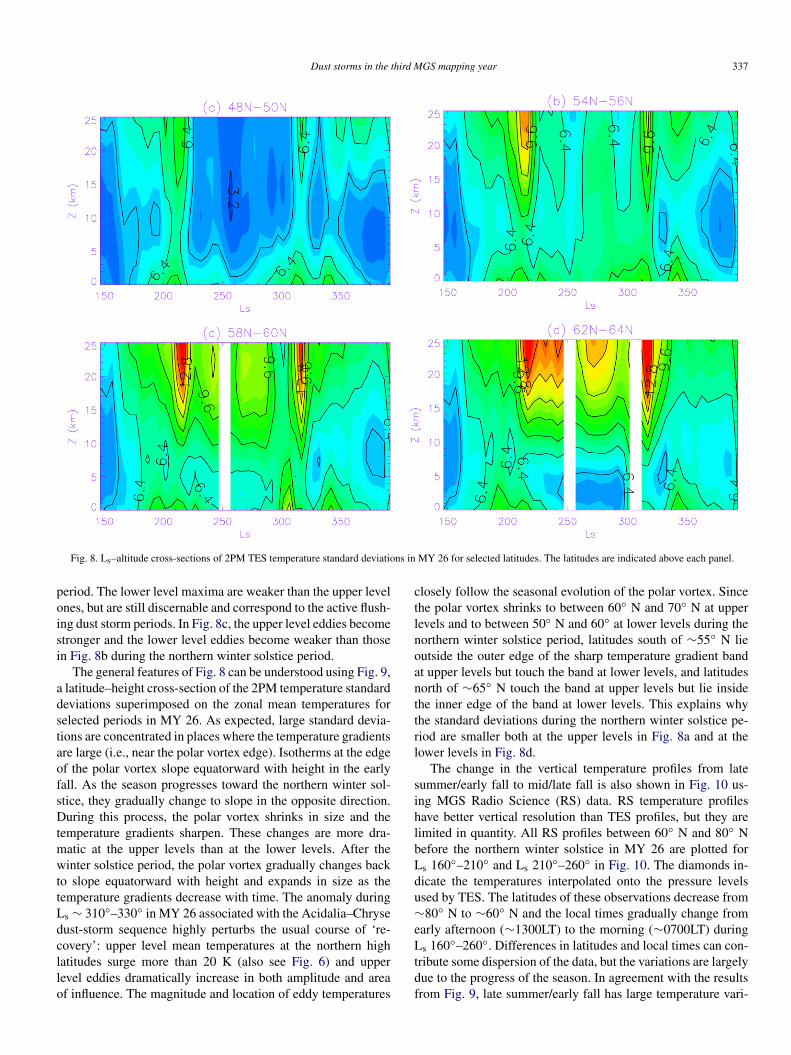
Dust storms in the third MGS mapping year 337

Fig. 8. Ls–altitude cross-sections of 2PM TES temperature standard deviations in MY 26 for selected latitudes. The latitudes are indicated above each panel.

period. The lower level maxima are weaker than the upper levelones, but are still discernable and correspond to the active flush-ing dust storm periods. In Fig. 8c, the upper level eddies becomestronger and the lower level eddies become weaker than thosein Fig. 8b during the northern winter solstice period.

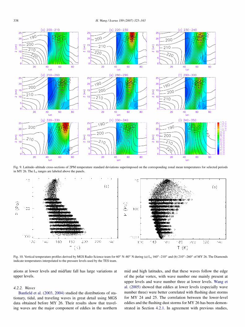
The general features of Fig. 8 can be understood using Fig. 9,a latitude–height cross-section of the 2PM temperature standarddeviations superimposed on the zonal mean temperatures forselected periods in MY 26. As expected, large standard devia-tions are concentrated in places where the temperature gradientsare large (i.e., near the polar vortex edge). Isotherms at the edgeof the polar vortex slope equatorward with height in the earlyfall. As the season progresses toward the northern winter sol-stice, they gradually change to slope in the opposite direction.During this process, the polar vortex shrinks in size and thetemperature gradients sharpen. These changes are more dra-matic at the upper levels than at the lower levels. After thewinter solstice period, the polar vortex gradually changes backto slope equatorward with height and expands in size as thetemperature gradients decrease with time. The anomaly duringLs ∼ 310◦–330◦ in MY 26 associated with the Acidalia–Chrysedust-storm sequence highly perturbs the usual course of ‘re-covery’: upper level mean temperatures at the northern highlatitudes surge more than 20 K (also see Fig. 6) and upperlevel eddies dramatically increase in both amplitude and areaof influence. The magnitude and location of eddy temperatures

closely follow the seasonal evolution of the polar vortex. Sincethe polar vortex shrinks to between 60◦ N and 70◦ N at upperlevels and to between 50◦ N and 60◦ at lower levels during thenorthern winter solstice period, latitudes south of ∼55◦ N lieoutside the outer edge of the sharp temperature gradient bandat upper levels but touch the band at lower levels, and latitudesnorth of ∼65◦ N touch the band at upper levels but lie insidethe inner edge of the band at lower levels. This explains whythe standard deviations during the northern winter solstice pe-riod are smaller both at the upper levels in Fig. 8a and at thelower levels in Fig. 8d.

The change in the vertical temperature profiles from latesummer/early fall to mid/late fall is also shown in Fig. 10 us-ing MGS Radio Science (RS) data. RS temperature profileshave better vertical resolution than TES profiles, but they arelimited in quantity. All RS profiles between 60◦ N and 80◦ Nbefore the northern winter solstice in MY 26 are plotted forLs 160◦–210◦ and Ls 210◦–260◦ in Fig. 10. The diamonds in-dicate the temperatures interpolated onto the pressure levelsused by TES. The latitudes of these observations decrease from∼80◦ N to ∼60◦ N and the local times gradually change fromearly afternoon (∼1300LT) to the morning (∼0700LT) duringLs 160◦–260◦. Differences in latitudes and local times can con-tribute some dispersion of the data, but the variations are largelydue to the progress of the season. In agreement with the resultsfrom Fig. 9, late summer/early fall has large temperature vari-

338 H. Wang / Icarus 189 (2007) 325–343

Fig. 9. Latitude–altitude cross-sections of 2PM temperature standard deviations superimposed on the corresponding zonal mean temperatures for selected periodsin MY 26. The Ls ranges are labeled above the panels.

Fig. 10. Vertical temperature profiles derived by MGS Radio Science team for 60◦ N–80◦ N during (a) Ls 160◦–210◦ and (b) 210◦–260◦ of MY 26. The Diamondsindicate temperatures interpolated to the pressure levels used by the TES team.

ations at lower levels and mid/late fall has large variations atupper levels.

4.2.2. WavesBanfield et al. (2003, 2004) studied the distributions of sta-

tionary, tidal, and traveling waves in great detail using MGSdata obtained before MY 26. Their results show that travel-ing waves are the major component of eddies in the northern

mid and high latitudes, and that these waves follow the edgeof the polar vortex, with wave number one mainly present atupper levels and wave number three at lower levels. Wang etal. (2005) showed that eddies at lower levels (especially wavenumber three) were better correlated with flushing dust stormsfor MY 24 and 25. The correlation between the lower-leveleddies and the flushing dust storms for MY 26 has been demon-strated in Section 4.2.1. In agreement with previous studies,

Dust storms in the third MGS mapping year 339

Fig. 11. Total power (K2) of eastward traveling waves with periods between 2 and 4 days and zonal wavenumber (a) m = 1, (b) m = 2, (c) m = 3.

the correlation breaks down above the first scale height. Ed-dies at upper levels are active during the winter solstice periods.Among the wide range of wave modes exhibited at upper lev-els, the wave number m = 1 waves with periods longer than∼6 days are dominant. This paper will concentrate on the wavesat lower levels.

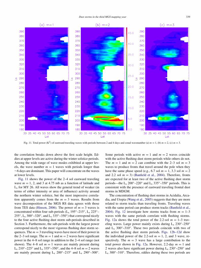
Fig. 11 shows the power of the 2–4 sol eastward travelingwave m = 1, 2, and 3 at 4.75 mb as a function of latitude andLs for MY 26. All waves show the general trend of weaker (interms of either intensity or area of influence) activity aroundthe northern winter solstice, but the most impressive correla-tion apparently comes from the m = 3 waves. Results fromwave decomposition of the MGS RS data agrees with thosefrom TES data (Hinson, 2006). The power of m = 3 waves isconcentrated within four sub-periods (Ls 195◦–215◦, Ls 225◦–255◦, Ls 300◦–320◦, and Ls 335◦–350◦) that correspond nicelyto the four active flushing dust storm sub-periods described inSection 3. Furthermore, the sub-periods with the largest powercorrespond nicely to the most vigorous flushing dust storm se-quences. The m = 3 traveling waves have most of their power inthe 2–3 sol range. The m = 1 and m = 2 waves have significantpower in the 4–8 sol range in addition to the 2–4 sol range (notshown). The 4–8 sol m = 1 waves are mainly present duringLs 210◦–225◦ and Ls 335◦–350◦, and the 4–8 sol m = 2 wavesare mainly present during Ls 200◦–215◦ and Ls 290◦–300◦.

Some periods with active m = 1 and m = 2 waves coincidewith the active flushing dust storm periods while others do not.The m = 1 and m = 2 can combine with the 2–3 sol m = 3waves to produce fronts that travel around the pole when theyhave the same phase speed (e.g., 6.7 sol m = 1, 3.3 sol m = 2and 2.2 sol m = 3) (Banfield et al., 2004). Therefore, frontsare expected for at least two of the active flushing dust stormperiods—the Ls 200◦–220◦ and Ls 335◦–350◦ periods. This isconsistent with the presence of eastward traveling frontal duststorms in MDGM.

The concentration of flushing dust storms in Acidalia, Arca-dia, and Utopia (Wang et al., 2005) suggests that they are morerelated to storm tracks than traveling fronts. Traveling waveswith the same period can produce storm tracks (Banfield et al.,2004). Fig. 12 investigate how storms tracks from m = 1–3waves with the same periods correlate with flushing storms.Fig. 12a shows the total power of the 2.2-sol m = 1–3 trav-eling waves. Large power mainly exists during Ls 230◦–250◦and Ls 300◦–310◦. These two periods coincide with two ofthe active flushing dust storm periods. Figs. 12b–12d showthe individual power of the 2.2-sol m = 1, 2, and 3 wave, re-spectively. The m = 3 wave has a large contribution to thetotal power shown in Fig. 12a. However, 2.2-day m = 1 and2 waves also have significant power during Ls 230◦–250◦ andLs 300◦–310◦. Therefore, eddies during these two periods are

340 H. Wang / Icarus 189 (2007) 325–343

Fig. 12. (a) Total power (K2) of eastward traveling 2.2-day m = 1, 2, and 3 waves. (b) Power of eastward traveling 2.2-day m = 1 wave. (c) Power of eastwardtraveling 2.2-day m = 2 wave. (d) Power of eastward traveling 2.2-day m = 3 wave. (e) Total power of eastward traveling 2.6-day m = 1, 2, and 3 waves. (f) Powerof eastward traveling 2.6-day m = 1 wave. (g) Power of eastward traveling 2.6-day m = 2 wave. (h) Power of eastward traveling 2.6-day m = 3 wave.

expected to exhibit storm track behavior resulting from the2.2-day traveling waves. Fig. 12e shows the total power ofthe 2.6-sol m = 1–3 waves. Large power mainly exists duringLs 200◦–210◦ and Ls 340◦–350◦ which lie within the other twoactive flushing storm periods. Figs. 12f–12h show the power

of 2.6-sol m = 1, 2, and 3 waves, respectively. In this case,both the m = 3 and m = 2 waves have significant contribu-tions to the total power shown in Fig. 12e, indicating stormtracks during these periods. In summary, Fig. 12 shows thatdifferent flushing dust storm periods are associated with storm

Dust storms in the third MGS mapping year 341

tracks made from different wave modes (e.g., 2.2-day wavesor 2.6-day waves). Furthermore, results in the previous para-graph and this paragraph combined show that storm trackscan coexist with fronts during certain flushing dust storm pe-riods.

5. Summary

The distribution of flushing dust storms in the third MGSmapping year (MY 26, 2003–2005) is presented in this pa-per. In agreement with the results for the previous two Marsyears, flushing dust storms are especially active before and af-ter a quiet period near the northern winter solstice during whichthere are no such storms. A special feature of MY 26 is thata statistically significant short gap in the seasonal distributionis observed in the pre- and post-solstice periods. The Ls 300◦–320◦ and Ls 200◦–220◦ sub-periods in MY 26 are the most ac-tive ones. Flushing dust storm sequences lead to dust accumula-tion in the southern hemisphere, resulting in significant pertur-bation to the large-scale structure of the atmosphere. The effectsof these major dust storms on the atmosphere are representedbest by different fields at different altitudes. At upper levels, theperturbed zonal mean temperatures as a function of latitude andLs show prominent dumbbell shapes with warmer temperaturesat the northern and southern mid and high latitudes indicatingan enhanced Hadley circulation due to increased dust loading.However, traveling waves at upper levels (m = 1 and 2) are gen-erally stronger during the northern winter solstice period, whichis opposite to the observed behavior of frontal dust storms. Atlower levels, the signatures of the major dust storms are not eas-ily recognizable in the zonal mean temperatures. However, theeastward m = 3 traveling waves with periods between 2 and 3days coincide with active frontal and flushing dust storms. Them = 3 waves combine with other waves of the same periods tomake storm tracks during each active sub-period. Sometimes,they also combine with other waves of the same phase speed tomake fronts.

6. Discussion

The m = 1 and 2 waves have deep vertical structures and aredominated by periods longer than 4 sols (Banfield et al., 2004).Modeling studies confirm that deeper structures are observedat longer wavelengths (Barnes et al., 1993; Wilson et al., 2002;Newman et al., 2002). Wilson et al. (2002) show that the m = 1wave is dominated by a period of 6.7 sol and can have signif-icantly longer period at higher altitudes. The m = 3 waves areconfined near the ground, have periods between 2 to 3 sols, andmainly occur away from the northern winter solstice. Hourdinet al. (1995) found a tendency for increased suppression of trav-eling wave activity during northern hemisphere winter solsticeseason as dust loading is increased in the LMD Mars GCM.Basu et al. (2006) simulated the transition between short andlong period traveling waves using the GFDL Mars GCM.

Multiple short active flushing dust storm sub-periods withinthe long pre- or post-solstice periods were conjectured by Wanget al. (2005) based on previous Viking and MGS observations.

They reasoned that major dust storms early in the long activeperiod could, through the intensification of the Hadley circu-lation, temporarily set the atmosphere into a state closer tothat typical of the northern winter solstice (Wang et al., 2005).This would briefly halt the formation of frontal and flushingdust storms. This is the first time that such sub-periods areclearly identified. The response of the atmosphere to the majordust storms in MY 26 shows clear signatures of an enhancedHadley circulation. The effects of the Ls 200◦–220◦ sequencelast for ∼10◦ Ls which is short enough for the return of flushingdust storms before the long winter solstice gap. The Ls 300◦–320◦ sequence involves more dust and produces stronger at-mospheric perturbations (e.g., polar warming), but its effectslast for only ∼10◦ Ls as well, probably because the seasonis departing from the winter solstice. Flushing dust storms re-turn after the hiatus and gradually move north with the band ofstrong eddies at the edge of the polar vortex. This is another ex-ample in support of the idea that the time of formation of majordust storms affects the duration and degree of their impact.

Throughout the northern fall and winter, the latitudinal bandaround the edge of the north polar vortex shows stronger eddiesthan other latitudes. The vertical distribution of eddy tempera-ture shows an upper level and a lower level maximum (Fig. 9),a feature simulated by the NASA AMES Mars GCM (Barneset al., 1993). The upper level eddies are dominated by wavenumber m = 1 and m = 2. The lower level eddies are domi-nated by wave number m = 2 and m = 3. The altitude with theminimum eddy temperature within the band varies between ∼5and ∼15 km and depends on the strength of the upper leveleddies: stronger upper level eddies (e.g., during the winter sol-stice period or major dust storms) lead to a lower height. Withthe strengthening of the temperature gradients at the polar vor-tex edge, the wind contours of the jet descend in altitude aswell (Banfield et al., 2003). The movement of the altitude ofthe weakest eddy temperature location appears to follow that ofthe 20 m/s contour, which is approximately the phase speed ofthe 2–3 sol wave number m = 3 wave, the 3–4 sol wave num-ber m = 2 wave, and the 6–7 sol wave number m = 1 wave.Wilson et al. (2002) comment on the eddy structure and its as-sociation with a “steering level” at the level of the 20 m/s zonalwind contour.

The three mapping years of MGS observations show a va-riety of paths for the development of major dust storms. TheMY 24 and MY 26 dust storm sequences are triggered by flush-ing dust storms that transport dust from the northern to thesouthern hemisphere through the Acidalia–Chryse or Utopiachannel. The MY 25 global dust storms are triggered by duststorms locally generated in or around Hellas basin. The sub-sequent development of these major events was examined bydata assimilation using the AOPP/LMD MGCM (Montaboneet al., 2005). Merging of dust storms (Cantor et al., 2001) oc-curred in all three Mars years. The observed number of merg-ings during the seasons examined is 12, 4, and 3 for years 1, 2,and 3, respectively, although the actual number could be largerbecause the MDGM only examine the early afternoon hours(∼2PM). The difference between the first and the other twoMars years could be real; however, it is possible that the major-

342 H. Wang / Icarus 189 (2007) 325–343

ity of merging events in different years occur at a different localtime, which could make MGS mapping Year 1 appear to havemore merging events. Newman et al. (2002) simulated Chryse-and Hellas-type dust storms with radiatively active dust trans-port and parameterized dust lifting in the AOPP/LMD MGCM.Their results showed that positive feedbacks between the at-mospheric state and threshold sensitive stress lifting could trig-ger further dust lifting once the initial dust storm formed. Thisis consistent with the observations that major dust storms are as-sociated with dust storm sequences that exhibit multiple centersof activity, with later dust lifting enhancing earlier lifting. Basuet al. (2006) also simulated Chryse- and Hella-type dust stormswith the GFDL MGCM. In agreement with observations, theyshowed that the simulated transient waves are weaker during thenorthern winter solstice period. They also state that the Chryse-type dust storms are larger at lower obliquities and can growinto global dust storms.

During the aerobraking and science phase of MGS (MY 23),TES observed two regional dust storms in the southern hemi-sphere. One occurred in Noachis during Ls 225◦–233◦ and theother occurred north of Argyre at Ls ∼ 309◦ (Smith et al.,2000). The time of occurrence is well within the active flush-ing dust storm periods. Based on the experience from MY 26,the locations are also within the reach of flushing dust stormsequences. Although the MY 23 regional dust storms are verylikely to be locally generated, there is a possibility that theycould be related to flushing dust storms. Unfortunately, noglobal maps were taken at the time to clarify the developmenthistories of these dust storms.

MGS observations show that the enhancement of the Hadleycirculation is accompanied by the suppression of lower leveltransient eddies (associated with frontal dust storms) and theamplification of upper level transient eddies at northern mid andhigh latitudes, suggesting that energy is re-partitioned betweendifferent circulation components. Using Viking data, Leovy etal. (1985) noticed that the circulation of the global dust stormyears was characterized by an enhanced Hadley circulation andsuppressed baroclinic waves. Haberle (1986) attempted to ex-plain the interannual variability of global dust storms basedon the idea that northern baroclinic waves would increase dustin the northern hemisphere which would suppress the Hadleycirculation and global dust storms. While the anti-correlationbetween the Hadley circulation and lower level baroclinic ed-dies is still true, dust initially raised in northern frontal duststorms can apparently travel to the southern hemisphere andlead to substantial enhancement of the Hadley circulation. Tran-sient eddies at northern mid and high latitudes are studied inthis paper because they are directly relevant to the frontal duststorms observed in images. Other circulation components, suchas the thermal tides and stationary waves, certainly change withseason and dust as well (Banfield et al., 2000, 2003; Lewis andBarker, 2005; Wilson and Richardson, 2000), but these topicsare beyond the scope of this paper.

Acknowledgments

The author would like to thank Phil James and an anony-mous reviewer for reviews, John Wilson and Chris Walker forcomments. This research project is supported by funding fromHarvard University.

References

Banfield, D., Conrath, B.J., Pearl, J.C., Smith, M.D., Christensen, P.R., 2000.Thermal tides and stationary waves on Mars as revealed by Mars GlobalSurveyor thermal emission spectrometer. J. Geophys. Res. 105, 9521–9537.

Banfield, D., Conrath, B.J., Smith, M.D., Christensen, P.R., Wilson, R.J.,2003. Forced waves in the martian atmosphere from MGS TES nadir data.Icarus 161, 319–345.

Banfield, D., Conrath, B.J., Gierasch, P.J., Wilson, R.J., Smith, M.D., 2004.Traveling waves in the martian atmosphere from MGS TES nadir data.Icarus 170, 365–403.

Barnes, J.R., 1980. Time spectral analysis of midlatitude disturbances in themartian atmosphere. J. Atmos. Sci. 37, 2002–2015.

Barnes, J.R., Pollack, J.B., Haberle, R.M., Leovy, C.B., Zurek, R.W., Lee, H.,Schaeffer, J., 1993. Mars atmospheric dynamics as simulated by the NASAAmes general circulation model. 2. Transient baroclinic eddies. J. Geophys.Res. 98, 3125–3148.

Basu, S., Wilson, R.J., Richardson, R.I., Ingersoll, A.P., 2006. Simulation ofspontaneous and variable global dust storms with the GFDL Mars GCM.J. Geophys. Res. 111, doi:10.1029/2005JE002660. E09004.

Cantor, B.A., James, P.B., Caplinger, M., Wolff, M.J., 2001. Martian duststorms: 1999 Mars Orbiter Camera observations. J. Geophys. Res. 106,23653–23687.

Haberle, R.M., 1986. Interannual variability of global dust storms on Mars.Science 234, 459–461.

Haberle, R.M., Pollack, J.B., Barnes, J.R., Zurek, R.W., Leovy, C.B., Murphy,J.R., Lee, H., Schaeffer, J., 1993. Mars atmospheric dynamics as simulatedby the NASA AMES general circulation model. 1. The zonal–mean circu-lation. J. Geophys. Res. 98, 3093–3123.

Hinson, D.P., 2006. Radio occultation measurements of transient eddies inthe northern hemisphere of Mars. J. Geophys. Res. 111, doi:10.1029/2005JE0026512. E05002.

Hourdin, F., Forget, F., Talagrand, O., 1995. The sensitivity of the martian sur-face pressure and atmospheric mass budget to various parameters: A com-parison between numerical simulations and Viking observations. J. Geo-phys. Res. 100, 5501–5523.

Jakosky, B.M., Martin, T.Z., 1987. Mars: North-polar atmospheric temperaturesduring dust storms. Icarus 72, 528–534.

Lewis, S.R., Barker, P.R., 2005. Atmospheric tides in a Mars general circulationmodel with data assimilation. Adv. Space Res. 36, 2162–2168.

Leovy, C.B., Tillman, J.E., Guest, W.R., Barnes, J.R., 1985. In: Hunt, G.E.(Ed.), Recent Advances in Planetary Meteorology. Cambridge Univ. Press,Cambridge, pp. 69–84.

Liu, J., Richardson, M.I., Wilson, R.J., 2003. An assessment of the global, sea-sonal, and interannual spacecraft record of martian climate in the thermalinfrared. J. Geophys. Res. 108, doi:10.1029/2002JE001921.

Montabone, L., Lewis, S.R., Read, P.L., 2005. Interannual variability of mar-tian dust storms in assimilation of several years of Mars global surveyorobservations. Adv. Space Res. 36, 2146–2155.

Newman, C.E., Lewis, S.R., Read, P.L., Forget, F., 2002. Modeling the mar-tian dust cycle. 2. Multi-annual radiatively active dust transport simulations.J. Geophys. Res. 107, doi:10.1029/2002JE001920.

Smith, M.D., 2004. Interannual variability in TES atmospheric observations ofMars during 1999–2003. Icarus 167, 148–165.

Smith, M.D., Pearl, J.C., Conrath, B.J., Christensen, P.R., 2000. Mars GlobalSurveyor Thermal Emission Spectrometer (TES) observations of dust opac-ity during aerobraking and science phasing. J. Geophys. Res. 105, 9539–9552.

Dust storms in the third MGS mapping year 343

Smith, M.D., Conrath, B.J., Pearl, J.C., Christensen, P.R., 2002. Thermal emis-sion spectrometer observations of martian planet-encircling dust storm2001A. Icarus 157, 259–263.

Strausberg, M.J., Wang, H., Richardson, M.I., Ewald, S.P., Toigo, A.D., 2005.Observations of the initiation and evolution of the 2001 Mars global duststorm. J. Geophys. Res. 110, doi:10.1029/2004JE002361.

Wang, H., Ingersoll, A.P., 2002. Martian clouds observed by Mars GlobalSurveyor Mars Orbiter Camera. J. Geophys. Res. 107, doi:10.1029/2001JE001815.

Wang, H., Richardson, M.I., Wilson, R.J., Ingersoll, A.P., Toigo, A.D., Zurek,R.W., 2003. Cyclones, tides, and the origin of a cross-equatorial dust stormon Mars. Geophys. Res. Lett. 30, doi:10.1029/2002GL016828.

Wang, H., Zurek, R.W., Richardson, M.I., 2005. Relationship between frontaldust storms and transient eddy activity in the northern hemisphere of Marsas observed by Mars Global Surveyor. J. Geophys. Res. 110, doi:10.1029/2005JE002423.

Wilson, R.J., 1997. A general circulation model simulation of the martian polarwarming. Geophys. Res. Lett. 24, 123–126.

Wilson, R.J., Richardson, M.I., 2000. The martian atmosphere during theViking mission, I. Infrared measurements of atmospheric temperature re-vised. Icarus 145, 555–579.

Wilson, R.J., Banfield, D., Conrath, B.J., Smith, M.D., 2002. Traveling wavesin the northern hemisphere of Mars. Geophys. Res. Lett. 29, doi:10.1029/2002GL014866.