Embed Size (px)
Citation preview

AFRL-RH-WP-TR-2020-0051
ASYMPTOTIC PERFORMANCE AND LEARNING CURVES IN MARKSMANSHIP EXPERIMENTS
Andrew D. Johnson, Jonathan Sagan, R. Michael Hinds Leidos
Grant Rousch
Henry M. Jackson Foundation
Michael Reddix Naval Medical Research Unit Dayton
FEBRUARY 2020 Interim Report
Distribution A. Approved for public release DESTRUCTION NOTICE – Destroy by any method that will prevent disclosure of contents or reconstruction of the document.
See additional restrictions described on inside pages
AIR FORCE RESEARCH LABORATORY 711TH HUMAN PERFORMANCE WING,
AIRMAN SYSTEMS DIRECTORATE, WRIGHT-PATTERSON AIR FORCE BASE, OH 45433
AIR FORCE MATERIEL COMMAND UNITED STATES AIR FORCE

NOTICE AND SIGNATURE PAGE Using Government drawings, specifications, or other data included in this document for any purpose other than Government procurement does not in any way obligate the U.S. Government. The fact that the Government formulated or supplied the drawings, specifications, or other data does not license the holder or any other person or corporation; or convey any rights or permission to manufacture, use, or sell any patented invention that may relate to them. This report was cleared for public release by the 88th Air Base Wing Public Affairs Office and is available to the general public, including foreign nationals. Copies may be obtained from the Defense Technical Information Center (DTIC) (http://www.dtic.mil). AFRL-RH-WP-TR-2020-0051 HAS BEEN REVIEWED AND IS APPROVED FOR PUBLICATION IN ACCORDANCE WITH ASSIGNED DISTRIBUTION STATEMENT
_______________________________ ________________________________ WILLIAM T. GREER, DR-IV, WUM RICHARD A. MCKINLEY Aircraft CBRN Survivability CRA Lead Airman Systems Directorate Airman Systems Directorate 711th Human Performance Wing 711th Human Performance Wing Air Force Research Laboratory Air Force Research Laboratory This report is published in the interest of scientific and technical information exchange, and its publication does not constitute the Government’s approval or disapproval of its ideas or findings.

REPORT DOCUMENTATION PAGE Form Approved OMB No. 0704-0188
The public reporting burden for this collection of information is estimated to average 1 hour per response, including the time for reviewing instructions, searching existing data sources, searching existing data sources, gathering and maintaining the data needed, and completing and reviewing the collection of information. Send comments regarding this burden estimate or any other aspect of this collection of information, including suggestions for reducing this burden, to Department of Defense, Washington Headquarters Services, Directorate for Information Operations and Reports (0704-0188), 1215 Jefferson Davis Highway, Suite 1204, Arlington, VA 22202-4302. Respondents should be aware that notwithstanding any other provision of law, no person shall be subject to any penalty for failing to comply with a collection of information if it does not display a currently valid OMB control number. PLEASE DO NOT RETURN YOUR FORM TO THE ABOVE ADDRESS.
1. REPORT DATE (DD-MM-YY) 2. REPORT TYPE 3. DATES COVERED (From - To) 28-02-20 Interim
4. TITLE AND SUBTITLE Asymptotic Performance and Learning Curves in Marksmanship Experiments
5a. CONTRACT NUMBER FA8650-16-D-6622 0001
5b. GRANT NUMBER
5c. PROGRAM ELEMENT NUMBER 00000F
6. AUTHOR(S) *Andrew D. Johnson, Jonathan Sagan, R. Michael Hinds **Grant Rousch ***Michael Reddix
5d. PROJECT NUMBER
5e. TASK NUMBER
5f. WORK UNIT NUMBER H0PF
7. PERFORMING ORGANIZATION NAME(S) AND ADDRESS(ES) 8. PERFORMING ORGANIZATION *Leidos **Henry M Jackson Foundation 1140 N. Eglin Parkway Shalimar, FL 32579
REPORT NUMBER
9. SPONSORING/MONITORING AGENCY NAME(S) AND ADDRESS(ES) 10. SPONSORING/MONITORING Air Force Materiel Command Air Force Research Laboratory 711th Human Performance Wing Airman Systems Directorate Airman Bioengineering Division Aircraft CBRN Survivability Branch Wright-Patterson AFB, OH 45433
***Naval Medical 2624 Q Street, Building 851, Area B Wright Patterson AFB, OH 45433
AGENCY ACRONYM(S) 711 HPW/RHBN 11. SPONSORING/MONITORING AGENCY REPORT NUMBER(S) AFRL-RH-WP-TR-2020-0051
12. DISTRIBUTION/AVAILABILITY STATEMENT Distribution A: Approved for public release. 88ABW-2020-2247 cleared on 13 July 2020
13. SUPPLEMENTARY NOTES
14. ABSTRACT This study investigated means by which the asymptotic level of performance for a marksmanship static-target shooting session may be calculated, as well as the development of learning curves based on asymptotic levels of performance from multiple sessions. This investigation focused on three aspects of marksmanship performance: accuracy and precision without a time constraint, speed-accuracy and visual search. In the accuracy and precision experiment, no significant degree of improvement was observed. In the speed-accuracy experiment, neither asymptotic performance nor learning curves could be computed based on these data, and no statistically significant correlation was found between time and shot distance from the center of the target. In the visual search experiment, results indicated that there were no significant changes in accuracy at any of the visual acuity levels. The results of these experiments will inform the design of future marksmanship performance experiments of a similar nature, while the methods described have potential utility in marksmanship training experiments and the comparison of performance with different weapons and ammunition, due to the reliable means provided for observing the asymptotic plateau of best sustained performance 15. SUBJECT TERMS
Asymptotic performance, learning curves, marksmanship, speed-accuracy, training 16. SECURITY CLASSIFICATION OF: 17. LIMITATION
OF ABSTRACT: SAR
18. NUMBER OF PAGES
398
19a. NAME OF RESPONSIBLE PERSON (Monitor) a. REPORT Unclassified
b. ABSTRACT Unclassified
c. THIS PAGE Unclassified
William Greer 19b. TELEPHONE NUMBER (Include Area Code) N/A
Standard Form 298 (Rev. 8-98) Prescribed by ANSI Std. Z39-18

i
TABLE OF CONTENTS
1 SUMMARY ........................................................................................................... 1 2 INTRODUCTION .................................................................................................. 3 3 METHODS AND MATERIALS .............................................................................. 5 3.1 Participant Recruitment and Screening ........................................................... 5 3.2 Indoor Simulated Marksmanship Trainer (ISMT) System ............................... 5 3.2.1 ISMT Data Output ........................................................................................... 8 3.2.2 Ballistics .......................................................................................................... 8 3.3 Experiments and Protocols ............................................................................. 9 3.3.1 Marksmanship Accuracy and Precision Experiment ....................................... 9 3.3.2 Marksmanship Speed-Accuracy Experiment ................................................ 11 3.3.3 Marksmanship Visual Search Experiment..................................................... 13 3.4 Statistical Analysis ........................................................................................ 15 3.4.1 Overview ....................................................................................................... 15 3.4.2 Marksmanship Accuracy and Precision Experiment ..................................... 16 3.4.3 Marksmanship Speed Accuracy Experiment................................................. 18 3.4.4 Marksmanship Visual Search Experiment..................................................... 19 3.5 Equipment ..................................................................................................... 19 3.5.1 Ocular Screening .......................................................................................... 19 3.5.2 Marksmanship Experiments .......................................................................... 19 4 RESULTS AND DISCUSSION ........................................................................... 20 4.1 Results .......................................................................................................... 20 4.1.1 Marksmanship Accuracy and Precision Experiment ..................................... 20 4.1.2 Marksmanship Speed-Accuracy Experiment ................................................ 58 4.1.3 Marksmanship Visual Search Experiment................................................... 101 4.2 Discussion................................................................................................... 104 4.2.1 Marksmanship Accuracy and Precision Experiment ................................... 104 4.2.2 Marksmanship Speed-Accuracy Experiment .............................................. 106 4.2.3 Marksmanship Visual Search Experiment................................................... 107 5 CONCLUSIONS ............................................................................................... 108 6 REFERENCES ................................................................................................. 109 LIST OF SYMBOLS, ABBREVIATIONS, AND ACRONYMS ...................................... 111 Appendix A .................................................................................................................. 112 Appendix B .................................................................................................................. 199 Appendix C .................................................................................................................. 364

ii
LIST OF FIGURES
Figure 1. ISMT Physical Configuration ............................................................................ 6 Figure 2. ISMT System in Use ........................................................................................ 7 Figure 3. ISMT Wireless M9 pistol................................................................................... 7 Figure 4. ISMT Wireless M4A1 Carbine .......................................................................... 8 Figure 5. Accuracy and Precision Experiment Target ................................................... 11 Figure 6. Speed-Accuracy Experiment Target .............................................................. 13 Figure 7. Tumbling E Target .......................................................................................... 15 Figure 8. Generalized Statistical Analysis Process ....................................................... 16 Figure 9. Experienced and Inexperienced Subjects Iterations to Pistol Asymptote ....... 21 Figure 10. Experienced and Inexperienced Subjects Iterations to Rifle Asymptote ...... 22 Figure 11. Pistol Iterations to Asymptote ....................................................................... 23 Figure 12. Rifle Iterations to Asymptote ........................................................................ 24 Figure 13. Iterations to Asymptote for Pistol and Rifle................................................... 25 Figure 14. Pistol Group Size for All Subjects ................................................................. 26 Figure 15. Pistol MPI to CZP Distance for All Subjects ................................................. 27 Figure 16. Pistol DCMS for all Subjects ........................................................................ 28 Figure 17. Pistol Mean Radius Data for All Subjects ..................................................... 29 Figure 18. Rifle Group Size Data for All Subjects .......................................................... 30 Figure 19. Rifle MPI to CZP Distance Data for All Subjects .......................................... 31 Figure 20. Rifle DCMS Data for All Subjects ................................................................. 32 Figure 21. Rifle Mean Radius Data for All Subjects ...................................................... 33 Figure 22. Experienced Subjects Pistol Group Size ...................................................... 34 Figure 23. Experienced Subjects Pistol MPI to CZP Distance ...................................... 35 Figure 24. Experienced Subjects Pistol DCMS ............................................................. 36 Figure 25. Experienced Subjects Pistol Mean Radius ................................................... 37 Figure 26. Inexperienced Subjects Pistol Group Size ................................................... 38 Figure 27. Inexperienced Subjects Pistol MPI to CZP Distance .................................... 39 Figure 28. Inexperienced Subjects Pistol DCMS ........................................................... 40 Figure 29. Inexperienced Subjects Pistol Mean Radius ................................................ 41 Figure 30. Experienced Subjects Rifle Group Size ....................................................... 42 Figure 31. Experienced Subjects Rifle MPI to CZP Distance ........................................ 43 Figure 32. Experienced Subjects Rifle DCMS ............................................................... 44 Figure 33. Experienced Subjects Rifle Mean Radius .................................................... 45 Figure 34. Experienced Subjects Rifle MR ANOVA Residuals QQ Plot ........................ 46 Figure 35. Inexperienced Subjects Rifle Group Size ..................................................... 47 Figure 36. Inexperienced Subjects Rifle MPI to CZP Distance ..................................... 48 Figure 37. Inexperienced Subjects Rifle DCMS ............................................................ 49 Figure 38. Inexperienced Subjects Rifle Mean Radius .................................................. 50 Figure 39. Experienced and Inexperienced Subjects Pistol Group Size ....................... 51 Figure 40. Experienced and Inexperienced Subjects Pistol MPI to CZP Distance ........ 52 Figure 41. Experienced and Inexperienced Subjects Pistol DCMS ............................... 53 Figure 42. Experienced and Inexperienced Subjects Pistol Mean Radius .................... 54 Figure 43. Experienced and Inexperienced Subjects Rifle Group Size ......................... 55 Figure 44. Experienced and Inexperienced Subjects Rifle MPI to CZP Distance .......... 56

iii
Figure 45. Experienced and Inexperienced Subjects Rifle DCMS ................................ 57 Figure 46. Experienced and Inexperienced Subjects Rifle Mean Radius ...................... 58 Figure 47. All Subjects IES - MPI to CZP Distance Based ............................................ 59 Figure 48. All Subjects RT - MPI to CZP Distance Based ............................................. 59 Figure 49. All Subjects Proportion Correct - MPI to CZP Distance Based ..................... 60 Figure 50. All Subjects IES - DCMS Based ................................................................... 61 Figure 51. All Subjects RT - DCMS Based .................................................................... 61 Figure 52. All Subjects Proportion Correct - DCMS Based ........................................... 62 Figure 53. All Subjects Five Quantile Day 2 1/MPI to CZP Distance ............................. 63 Figure 54. All Subjects Five Quantile Day 2 1/DCMS.................................................... 64 Figure 55. All Subjects Five Quantile Day 3 1/MPI to CZP Distance ............................. 65 Figure 56. All Subjects Five Quantile Day 3 1/DCMS.................................................... 66 Figure 57. All Subjects Five Quantile Day 41/MPI to CZP Distance .............................. 67 Figure 58. All Subjects Five Quantile Day 4 1/DCMS.................................................... 68 Figure 59. All Subjects Five Quantile Day 5 1/MPI to CZP Distance ............................. 69 Figure 60. All Subjects Five Quantile Day 5 1/DCMS.................................................... 70 Figure 61. All Subjects Six Quantile Day 2 1/MPI to CZP Distance .............................. 71 Figure 62. All Subjects Six Quantile Day 2 1/DCMS ..................................................... 72 Figure 63. All Subjects Six Quantile Day 3 1/MPI to CZP Distance .............................. 73 Figure 64. All Subjects Six Quantile Day 3 1/DCMS ..................................................... 74 Figure 65. All Subjects Six Quantile Day 41/MPI to CZP Distance ............................... 75 Figure 66. All Subjects Six Quantile Day 4 1/DCMS ..................................................... 76 Figure 67. All Subjects Six Quantile Day 5 1/MPI to CZP Distance .............................. 77 Figure 68. All Subjects Six Quantile Day 5 1/DCMS ..................................................... 78 Figure 69. All Subjects Quantile 1 of 5 1/MPI to CZP Distance ..................................... 79 Figure 70. All Subjects Quantile 2 of 5 1/MPI to CZP Distance Results ........................ 80 Figure 71. All Subjects Quantile 3 of 5 1/MPI to CZP Distance Results ........................ 81 Figure 72. All Subjects Quantile 4 of 5 1/MPI to CZP Distance Results ........................ 82 Figure 73. All Subjects Quantile 5 of 5 1/MPI to CZP Distance Results ........................ 83 Figure 74. All Subjects Quantile 1 of 5 1/DCMS Results ............................................... 84 Figure 75. All Subjects Quantile 2 of 5 1/DCMS Results ............................................... 85 Figure 76. All Subjects Quantile 3 of 5 1/DCMS Results ............................................... 86 Figure 77. All Subjects Quantile 4 of 5 1/DCMS Results ............................................... 87 Figure 78. All Subjects Quantile 5 of 5 1/DCMS Results ............................................... 88 Figure 79. All Subjects Quantile 1 of 6 1/MPI to CZP Distance Results ........................ 89 Figure 80. All Subjects Quantile 2 of 6 1/MPI to CZP Distance Results ........................ 90 Figure 81. All Subjects Quantile 3 of 6 1/MPI to CZP Distance Results ........................ 91 Figure 82. All Subjects Quantile 4 of 6 1/MPI to CZP Distance Results ........................ 92 Figure 83. All Subjects Quantile 5 of 6 1/MPI to CZP Distance Results ........................ 93 Figure 84. All Subjects Quantile 6 of 6 1/MPI to CZP Distance Results ........................ 94 Figure 85. All Subjects Quantile 1 of 6 1/DCMS Results ............................................... 95 Figure 86. All Subjects Quantile 2 of 6 1/DCMS Results ............................................... 96 Figure 87. All Subjects Quantile 3 of 6 1/DCMS Results ............................................... 97 Figure 88. All Subjects Quantile 4 of 6 1/DCMS Results ............................................... 98 Figure 89. All Subjects Quantile 5 of 6 1/DCMS Results ............................................... 99 Figure 90. All Subjects Quantile 6 of 6 1/DCMS Results ............................................. 100

iv
Figure 91. Subjects VS01-VS10 Acuity A Hit Proportions ........................................... 102 Figure 92. Subjects VS01-VS10 Acuity B Hit Proportions ........................................... 102 Figure 93. Subjects VS01-VS10 Acuity C Hit Proportions ........................................... 103 Figure 94. Subjects VS01-VS10 Acuity D Hit Proportions ........................................... 103

v
LIST OF TABLES
Table 1. Iterations to Reach Pistol Asymptote Shapiro-Wilk Test Results .................................22 Table 2. Iterations to Reach Rifle Asymptote Shapiro-Wilk Test Results ...................................24 Table 3. Pistol and Rifle Iterations to Asymptote Shapiro-Wilk Test Results ..............................25 Table 4. All Subjects Pistol Group Size Shapiro-Wilk Test Results ............................................26 Table 5. All Subjects Pistol MPI to CZP Distance Shapiro-Wilk Test Results ............................27 Table 6. All Pistol Subjects DCMS Shapiro-Wilk Test Results ...................................................28 Table 7. All Subjects Pistol Mean Radius Shapiro-Wilk Test Results ........................................29 Table 8. All Subjects Rifle Group Size Shapiro-Wilk Test Results .............................................30 Table 9. All Subjects Rifle MPI to CZP Distance Shapiro-Wilk Test Results ..............................31 Table 10. All Subjects Rifle DCMS Shapiro-Wilk Test Results ..................................................32 Table 11. All Subjects Rifle Mean Radius Shapiro-Wilk Test Results ........................................33 Table 12. Experienced Subjects Pistol Group Size Shapiro-Wilk Test Results ..........................34 Table 13. Experienced Subjects Pistol MPI to CZP Distance Shapiro-Wilk Test Results ...........35 Table 14. Experienced Subjects Pistol MPI to CZP Distance Dunn's Test Results ....................35 Table 15. Experienced Subjects Pistol DCMS Shapiro-Wilk Test Results .................................36 Table 16. Experienced Subjects Pistol Mean Radius Shapiro-Wilk Test Results .......................37 Table 17. Inexperienced Subjects Pistol Group Size Shapiro-Wilk Test Results .......................38 Table 18. Inexperienced Subjects Pistol MPI to CZP Distance Shapiro-Wilk Test Results ........39 Table 19. Inexperienced Subjects Pistol DCMS Shapiro-Wilk Test Results ...............................40 Table 20. Inexperienced Subjects Pistol Mean Radius Shapiro-Wilk Test Results ....................41 Table 21. Experienced Subjects Rifle Group Size Shapiro-Wilk Test Results ...........................42 Table 22. Experienced Subjects Rifle MPI to CZP Distance Shapiro-Wilk Test Results ............43 Table 23. Experienced Subjects Rifle DCMS Shapiro-Wilk Test Results ...................................44 Table 24. Experienced Subjects Rifle Mean Radius Shapiro-Wilk Test Results ........................45 Table 25. Inexperienced Subjects Rifle Group Size Shapiro-Wilk Test Results .........................46 Table 26. Inexperienced Subjects Rifle MPI to CZP Distance Shapiro-Wilk Test Results ..........47 Table 27. Inexperienced Subjects Rifle DCMS Shapiro-Wilk Test Results ................................48 Table 28. Inexperienced Subjects Rifle Mean Radius Shapiro-Wilk Test Results ......................49 Table 29. Inexperienced Subjects Rifle Mean Radius REGWQ Test Results ............................50 Table 30. Experienced and Inexperienced Subjects Pistol Group Size Shapiro-Wilk Test Results .................................................................................................................................................51 Table 31. Experienced and Inexperienced Subjects Pistol Group Size REGWQ Test Results ..51 Table 32. Experienced and Inexperienced Subjects Pistol MPI to CZP Distance Shapiro-Wilk Test Results ......................................................................................................................................52 Table 33. Experienced and Inexperienced Subjects Pistol MPI to CZP Distance Dunn's Test Results ......................................................................................................................................52 Table 34. Experienced and Inexperienced Subjects Pistol DCMS Shapiro-Wilk Test Results ...53 Table 35. Experienced and Inexperienced Subjects Pistol Mean Radius Shapiro-Wilk Test Results .................................................................................................................................................54 Table 36. Experienced and Inexperienced Subjects Pistol Mean Radius REGWQ Test Results .................................................................................................................................................54 Table 37. Experienced and Inexperienced Subjects Rifle Group Size Shapiro-Wilk Test Results .................................................................................................................................................55 Table 38. Experienced and Inexperienced Subjects Rifle MPI to CZP Distance Shapiro-Wilk Test Results ......................................................................................................................................56 Table 39. Experienced and Inexperienced Subjects Rifle DCMS Shapiro-Wilk Test Results .....57 Table 40. Experienced and Inexperienced Subjects Rifle Mean Radius Shapiro-Wilk Test Results .................................................................................................................................................58

vi
Table 41. Experienced and Inexperienced Subjects Rifle Mean Radius REGWQ Test Results .58 Table 42. All Subjects Day 2 Five Quantile 1/MPI to CZP Distance Shapiro-Wilk Test Results .62 Table 43. All Subjects Day 2 Five Quantile 1/DCMS Shapiro-Wilk Test Results ........................63 Table 44. All Subjects Day 3 Five Quantile 1/MPI to CZP Distance Shapiro-Wilk Test Results .64 Table 45. All Subjects Day 3 Five Quantile 1/DCMS Shapiro-Wilk Test Results ........................65 Table 46. All Subjects Day 4 Five Quantile 1/MPI to CZP Distance Shapiro-Wilk Test Results .66 Table 47. All Subjects Day 4 Five Quantile 1/DCMS Shapiro-Wilk Test Results ........................67 Table 48. All Subjects Day 5 Five Quantile 1/MPI to CZP Distance Shapiro-Wilk Test Results .68 Table 49. All Subjects Day 5 Five Quantile 1/DCMS Shapiro-Wilk Test Results ........................69 Table 50. All Subjects Five Quantile Day 5 1/DCMS Distance Dunn’s Test Results ..................70 Table 51. All Subjects Day 2 Six Quantile 1/MPI to CZP Distance Shapiro-Wilk Test Results ...71 Table 52. All Subjects Day 2 Six Quantile 1/DCMS Shapiro-Wilk Test Results .........................72 Table 53. All Subjects Day 3 Six Quantile 1/MPI to CZP Distance Shapiro-Wilk Test Results ...73 Table 54. All Subjects Day 3 Six Quantile 1/DCMS Shapiro-Wilk Test Results .........................74 Table 55. All Subjects Day 4 Six Quantile 1/MPI to CZP Distance Shapiro-Wilk Test Results ...75 Table 56. All Subjects Day 4 Six Quantile 1/DCMS Shapiro-Wilk Test Results .........................76 Table 57. All Subjects Day 5 Six Quantile 1/MPI to CZP Distance Shapiro-Wilk Test Results ...77 Table 58. All Subjects Day 5 Six Quantile 1/DCMS Shapiro-Wilk Test Results .........................78 Table 59. All Subjects Quantile 1 of 5 1/MPI to CZP Distance Shapiro-Wilk Test Results .........79 Table 60. All Subjects Quantile 2 of 5 1/MPI to CZP Distance Shapiro-Wilk Test Results .........80 Table 61. All Subjects Quantile 3 of 5 1/MPI to CZP Distance Shapiro-Wilk Test Results .........81 Table 62. All Subjects Quantile 4 of 5 1/MPI to CZP Distance Shapiro-Wilk Test Results .........82 Table 63. All Subjects Quantile 5 of 5 1/MPI to CZP Distance Shapiro-Wilk Test Results .........83 Table 64. All Subjects Quantile 1 of 5 1/DCMS Shapiro-Wilk Test Results ................................84 Table 65. All Subjects Quantile 2 of 5 1/DCMS Shapiro-Wilk Test Results ................................85 Table 66. All Subjects Quantile 3 of 5 1/DCMS Shapiro-Wilk Test Results ................................86 Table 67. All Subjects Quantile 4 of 5 1/DCMS Shapiro-Wilk Test Results ................................87 Table 68. All Subjects Quantile 5 of 5 1/DCMS Shapiro-Wilk Test Results ................................88 Table 69. All Subjects Quantile 1 of 6 1/MPI to CZP Distance Shapiro-Wilk Test Results .........89 Table 70. All Subjects Quantile 2 of 6 1/MPI to CZP Distance Shapiro-Wilk Test Results .........90 Table 71. All Subjects Quantile 3 of 6 1/MPI to CZP Distance Shapiro-Wilk Test Results .........91 Table 72. All Subjects Quantile 4 of 6 1/MPI to CZP Distance Shapiro-Wilk Test Results .........92 Table 73. All Subjects Quantile 5 of 6 1/MPI to CZP Distance Shapiro-Wilk Test Results .........93 Table 74. All Subjects Quantile 6 of 6 1/MPI to CZP Distance Shapiro-Wilk Test Results .........94 Table 75. All Subjects Quantile 1 of 6 1/DCMS Shapiro-Wilk Test Results ................................95 Table 76. All Subjects Quantile 2 of 6 1/DCMS Shapiro-Wilk Test Results ................................96 Table 77. All Subjects Quantile 3 of 6 1/DCMS Shapiro-Wilk Test Results ................................97 Table 78. All Subjects Quantile 4 of 6 1/DCMS Shapiro-Wilk Test Results ................................98 Table 79. All Subjects Quantile 5 of 6 1/DCMS Shapiro-Wilk Test Results ................................99 Table 80. All Subjects Quantile 6 of 6 1/DCMS Shapiro-Wilk Test Results .............................. 100 Table 81. All Subjects Correlation Results .............................................................................. 101 Table 82. Subjects VS01-VS10 Acuity Hit Proportions ............................................................ 101 Table 83. Subjects VS01-VS10 Daily Hit Proportions .............................................................. 101
1 Distribution A: Approved for public release. 88ABW-2020-2247, cleared on 13 July 2020
1 SUMMARY
In human factors experiments that investigate marksmanship behavior, repeated execution of a course of fire can lead to improvements in performance. Removing this potential source of nuisance variance from experiment treatment effects is a critical step in interpreting and confidently generalizing findings from marksmanship performance studies. A reliable method for the experimental observation of asymptote development will achieve this goal and could also provide marksmanship instructors a valuable method for ascertaining student achievement of a training criterion-of-performance and the level of practice needed to maintain a desired level of proficiency. This study investigated means by which the asymptotic level of performance for a marksmanship session may be calculated, as well as the development of learning curves based on asymptotic levels of performance from multiple sessions. This investigation focused on three aspects of marksmanship performance: accuracy and precision without a time constraint, speed-accuracy and visual search.
In the accuracy and precision experiment, performance with the M9 pistol and M4A1 carbine was assessed over 4 days, during which 30 iterations were fired with each weapon daily. Subjects were placed into one of two groups: experienced and inexperienced. Experienced subjects were those who had served in the military or law enforcement or who had participated in competitive marksmanship or hunting, while inexperienced subjects had none of the aforementioned experience. During each of the 30 iterations, subjects fired 3 shots at a simple cross shaped target. Asymptotic performance was determined by first computing the 5 iteration running variance of the area of dispersion, which was the smallest rectangle able to encompass all of the shots during a given iteration. Once the 5 iteration running variance was computed, the asymptotic dataset was determined by selecting the 2 lowest points on the curve that were also the closest in value, which were designated points ni and ni+1. The iterations comprising the asymptotic dataset, ni-5 through ni+1, were then compared using the appropriate statistical methods. The results of the accuracy and precision experiment indicated that, under the conditions of the experiment, performance in terms of accuracy and precision would not be expected to improve over 4 days of data collection.
In the speed-accuracy experiment, subjects who successfully completed the qualification course of fire were required to shoot 30 iterations of 3 shots at a silhouette target using the M4A1. Time and measures of accuracy were collected, and based on these data, the Inverse Efficiency Scores (IES) and Conditional Accuracy Function (CAF) were calculated, as well as simple correlation between time and shot distance from the center of the target. Neither asymptotic performance nor learning curves could be computed based on these data, and no statistically significant correlation was found between time and shot distance from the center of the target.
In the visual search experiment, subjects who successfully completed the qualification course of fire were required to engage tumbling E targets with the M4A1 at 4 distinct Snellen visual acuities (20/204, 20/165, 20/114 and 20/84). Asymptotic performance was computed by determining the proportion of targets hit for each acuity with a chi-squared

2 Distribution A: Approved for public release. 88ABW-2020-2247, cleared on 13 July 2020
test of proportions and 95% confidence intervals, with learning curves being determined by plotting each day’s asymptotic performance on a graph. Through the 4 days of data collection, results indicated that there were no significant changes in accuracy at any of the visual acuity levels.
The results of these experiments will inform the design of future marksmanship performance experiments. Since no significant improvement in accuracy and precision performance or visual search performance is likely to be observed during 4 days of data collection, future experiments may be designed with one day for baseline performance and three days for the addition of treatments, provided the participants have at least a minimal level of marksmanship proficiency at the outset. One such notional design would include a baseline data collection day, a day with pilocarpine treatment, a day with the addition of MOPP-4, and a final day with both pilocarpine treatment and MOPP-4.

3 Distribution A: Approved for public release. 88ABW-2020-2247, cleared on 13 July 2020
2 INTRODUCTION
When a task is performed or practiced repeatedly, there is usually a degree of improvement in the metrics by which performance of that task is measured. In psychology, economics and operations management, such improvement over time is represented through a learning curve.1,2,3 While task performance and learning curves have been studied for elite chess players, race car drivers, construction workers and surgeons, a literature search found no directly relevant research concerning rifle and pistol marksmanship performance and learning curves in peer reviewed journals in recent years.3,4,5,6
Learning curves for rifle and pistol marksmanship performance and target identification are of particular importance to any experiments in which the effects of a treatment on performance are to be evaluated. In such experiments, test subjects’ performance, in terms of accuracy and precision, is likely to improve during their participation (a potential source of extraneous variance). Another dimension of marksmanship performance that may potentially improve over the course of the experiments is accuracy under a time constraint. As with any task having a cognitive component, the test subject’s accuracy will likely decrease as the time constraint becomes more restrictive.7 Conversely, accuracy under such circumstances can be improved at the expense of time, but the accuracy gains realized will eventually show diminishing returns.8 As a result of improvements in any of these dimensions of marksmanship performance, there is the potential for additional variance to be introduced into future test data, which may mask or amplify the effects of the treatment in question on performance.
In general, learning curves consider a test subject’s initial performance level with respect to a metric, such as a) the number of practice iterations, b) the test subject’s performance level during each practice iteration, c) the change in performance level, and d) the rate of change in performance level.3,4,9 Although most learning curves incorporate the same fundamental variables, the functions that define them and the resulting shapes of the curves, as well as their predictive validity, can differ significantly.2,9,10 One way in which learning curves can be described is through the power law, the simplest form of which is shown in equation 1, where T is the measure of performance, a is the curve’s starting point, P is the number of iterations, and b is the rate at which performance improves.4
T = a Pb (1)
While some investigators have asserted that the power law is universal in nature, others have disagreed because much of the research that supports the power law is based on the fitting of averaged data of many test subjects.11 Thus, learning curves based on the power law will not necessarily describe individual learning curves, due in part to individual differences (e.g., novice vs expert marksmen).12 Among such individual differences are punctuated learning dynamics, which appear as

4 Distribution A: Approved for public release. 88ABW-2020-2247, cleared on 13 July 2020
improvements followed by plateaus, which are in turn followed by improvements, among other features.13 Another critical drawback to the power law is the fact that some tasks with both motor and cognitive components, such as surgical procedures, have learning curves that do not conform to the smooth curve produced by the power law, but are instead linear, logarithmic, or exponential.10 Therefore, while the power law does have a long history of application to learning curves for a wide variety of tasks, it is not necessarily suited to the evaluation of individual learning curves or to tasks with both cognitive and motor components, such as marksmanship. It was thus the purpose of this study to evaluate marksmanship metrics in static and visual search targeting scenarios in order to determine the most suitable learning curve model for rifle and pistol performance, so that future CBRN related human performance studies may be conducted without the additional variance introduced by learning curves.
As this report will describe, this study has fulfilled its stated objectives and has demonstrated for the first time reliable methods for determining asymptotic performance and developing learning curves for multiple dimensions of marksmanship performance. These methods have potential utility in the development of courses of fire for military and law enforcement personnel as well as competitive shooters. Using the methods described, the best sustained, or asymptotic, level of performance for a given shooter during a training session can be reliably determined, enabling the development of training programs specific to the individual. Other potential applications include the determination of the amount and frequency of practice required to maintain proficiency and the comparison of performance with different weapons, modifications to weapons or types ammunition. Through application of these methods, investigators and trainers may enhance the statistical rigor of their evaluations.
5 Distribution A: Approved for public release. 88ABW-2020-2247, cleared on 13 July 2020
3 METHODS AND MATERIALS
3.1 Participant Recruitment and Screening
The recruiting goal for the study was 40 participants in order to obtain a total sample of 30 for the experiments. Recruitment and participation were conducted in accordance with a Naval Medical Research Unit Dayton (NAMRU-D) Institutional Review Board approved human subjects research protocol (NAMRUD.2018.0001-Learning Curves and Asymptotic Performance for Simulated Rifle and Pistol Marksmanship and Visual Search Tasks). Participants were recruited through email, word of mouth, posted flyers and advertisements in the Wright Patterson Air Force Base newspaper. Because the research was determined to involve no greater than minimum risk, active duty or retired military, federal employees and civilians were actively recruited. In order to be considered for inclusion in any of the experiments, participants were required to be between the ages of 18 and 40, in good overall health and have vision best corrected to 20/20 for both distant and near vision with glasses or contact lenses. Participants were further required to have a normal slit lap examination and intraocular pressure. Specific exclusion criteria included vision not correctable to 20/20 at distance or near, intraocular pressure outside of the normal limits of 10-21 mm Hg, a history of retinal detachment and the use of toric contact lenses, bifocals or progressive lenses.
3.2 Indoor Simulated Marksmanship Trainer (ISMT) System
In order to conduct the experiments with both safety and fidelity, a Meggitt Training Systems M100 ISMT system was chosen. The ISMT, variants of which are used in the Marine Corps as well as numerous law enforcement agencies, was installed in the Naval Medical Research Unit-Dayton Laser Laboratory. The projector and detection camera were positioned 7 ft (2.1 m) 7 in. (17.8 cm) and 7 ft (2.1 m) 1.5 in. (3.8 cm) above the floor respectively, and 15 ft (4.6 m) away from the screen. The screen measured 8 ft (2.4 m) by 8 ft (2.4 m) and was a Laservision model BC4.F5P01.5003. The system’s physical configuration is shown in Figures 1 and 2, and the weapons employed are shown in Figures 3 and 4.

6 Distribution A: Approved for public release. 88ABW-2020-2247, cleared on 13 July 2020
ISMT Computer
Weapons Locker
ISMT Projector and
Camera
Screen
Weapons Charging Station
Figure 1. ISMT Physical Configuration

7 Distribution A: Approved for public release. 88ABW-2020-2247, cleared on 13 July 2020
Figure 2. ISMT System in Use
Figure 3. ISMT Wireless M9 pistol

8 Distribution A: Approved for public release. 88ABW-2020-2247, cleared on 13 July 2020
Figure 4. ISMT Wireless M4A1 Carbine
As its name implies, the ISMT was designed for training, rather than human performance experiments. As a result, the pre-installed training courses of fire were not optimal, requiring researchers to use the system’s course authoring functionality to develop specialized courses of fire for all experiments. Among the parameters specified for each experiment were data output, ballistics, pass and fail criteria, target types, and visual and auditory cues. Specific aspects of each custom programmed course of fire will be discussed in subsequent sections.
3.2.1 ISMT Data Output
ISMT data output settings required special attention due to the system’s intended application as a training, rather than research, system. The default data export settings included basic marksmanship results such as group size, the group’s mean point of impact (MPI) and the score. While these data provided some useful information, they did not allow for the computation of many of the metrics which were required. In order to collect the required data, the ISMT was configured to consider each individual shot as a group. As a result, the system provided X and Y data, as well as timing for each shot.
3.2.2 Ballistics
By default, the ISMT incorporates ballistics specific to the weapons which are connected to the system and their standard ammunition. The standard zeroing distance

9 Distribution A: Approved for public release. 88ABW-2020-2247, cleared on 13 July 2020
is 300 yards for the M4A1 carbine and 10 yards for the M9 pistol. While ballistics, particularly with the M4A1 carbine, is very helpful in bringing fidelity to the ISMT, its use in human performance experimentation introduces potential variance because sights must be adjusted to reflect the range to the simulated target, and the M4A1 carbine’s sights allow for range adjustments only in increments of 100 yards, thus limiting the types, sizes, and distances of targets in the experiment, and introducing potential variance because of differences in skill level. Since such variance would likely have adverse effects on data collection, the ISMT was configured such that ballistics were not incorporated into the simulated marksmanship. This was accomplished by turning off the ballistics and dispersion options in the ISMT lanes training weapon menu.
3.3 Experiments and Protocols
The study consisted of three distinct experiments. The first experiment investigated the accuracy and precision aspects of marksmanship performance. The second experiment investigated the speed-accuracy aspect of marksmanship performance. The third experiment investigated the visual search aspect of marksmanship performance. Each experiment’s protocols will be described in the paragraphs that follow.
3.3.1 Marksmanship Accuracy and Precision Experiment
The marksmanship accuracy and precision experiment was the first to be completed. In this experiment, accuracy and precision in marksmanship against static targets with no time limit were the focus.
3.3.1.1 Objectives and Hypotheses
The objectives of the marksmanship accuracy and precision experiment were to investigate multiple aspects of asymptotic performance with the M9 pistol and the M4A1 carbine. The first aspect of asymptotic performance to be investigated was the influence of test subject experience level on the number of iterations required to reach an asymptotic level of performance during a session. This aspect was investigated because it was not known if inexperienced subjects would achieve a measurable asymptote and because it was not known if 30 iterations would be a suitable number of iterations. The next aspect of asymptotic performance to be investigated concerned the potential for the number of iterations required for a subject to reach asymptote decreasing over time. This aspect was investigated because such a decrease would represent a learning effect. The next aspect to be investigated was the difference in the number of iterations required to reach asymptote with the M9 pistol vs the M4A1 carbine. This aspect was investigated because of the potential for the differences in shooting a pistol versus shooting a rifle, such as weapon weight and trigger pull, to influence the number of iterations required to reach asymptote, and thus the number of iterations required to collect meaningful data in future experiments. The final aspect of asymptotic performance to be investigated was that the level of asymptotic performance would change over time. This aspect was investigated because a change in the level of asymptotic performance, in particular one indicative of improvement, would represent an improvement and could be represented as

10 Distribution A: Approved for public release. 88ABW-2020-2247, cleared on 13 July 2020
a learning curve.
In order to meet the objectives of this experiment, the following hypotheses were tested:
• Hypothesis 1: The number of iterations required to reach asymptote is dependent upon the experience level of the subject, with more experienced subjects requiring fewer iterations;
• Hypothesis 2: The number of iterations required for a subject to reach asymptote will decrease over time;
• Hypothesis 3: The number of iterations required to reach asymptote will be significantly different for rifle and pistol;
• Hypothesis 4: The level of asymptotic performance will improve to a small but significant extent.
The independent variables were marksmanship experience, weapon used (i.e., M4A1 or M9) and day of participation. Dependent variables included raw marksmanship performance and derived marksmanship performance metrics: single-target accuracy, single-target group size, iterations to asymptote, duration of asymptote and to central zero point (CZP) distance.
3.3.1.2 Design and Protocol
The experiment was a mixed design, with test subjects divided into two levels based on their level of marksmanship experience. The experienced level consisted of those test subjects who had received M9 pistol and/or M4A1 carbine training in the past, as well as those who had previous firearms experience through hunting, competition, or general marksmanship. The test subject sample consisted of 10 test subjects, half of whom were experienced, and half of whom were inexperienced. Due to the inability to properly collect data on the first four subjects, however, the subject sample size was limited to 6.
All subjects received orientation training on day 1. During the orientation training, subjects were instructed on basic weapons safety, proper shooting stances and experimental procedures. After instruction on day 1, subjects completed one course of fire with each weapon during which researchers provided basic marksmanship coaching. Coaching consisted of corrections to problems diagnosed by observation as well as by the ISMT’s barrel trace function, which provided feedback on muzzle movement immediately before, during and immediately after the trigger was pulled. After completion of firing, subjects were instructed to avoid practicing marksmanship skills outside of the experiment as well as changes to their consumption of caffeine, tobacco, alcohol, or prescription or over the counter drugs for the duration of the experiment. On days 2 through 5, subjects completed one course of fire with each weapon, with a 30 minute rest between weapons. The order of weapon use was counterbalanced.
The M4A1 course of fire consisted of 30 iterations during which the subject would fire 3 shots at a battlesight zero (BZO) target (a simple high-contrast cross-hair image), an

11 Distribution A: Approved for public release. 88ABW-2020-2247, cleared on 13 July 2020
example of which is shown in Figure 5, placed at a simulated distance of 25 yards. Subjects were not given a time limit for each iteration, and were instructed to strive for both accuracy and precision by aiming each shot at the center of the target to the best of their ability. The M9 course of fire also consisted of 30 iterations during which the subject would fire 3 shots at a target similar to that of the M4A1 course of fire, but placed at a simulated range of 10 yards. As with the M4A1 course of fire, there were no time limits imposed. In both courses of fire, subjects were given a 30 second rest period between iterations, during which researchers collected the X and Y coordinates of each shot fired during that iteration. If data for one or more shots in an iteration data were not available due to an ISMT or weapon malfunction, subjects completed additional 3 shot iterations as needed so that subject produced a complete dataset of 30 iterations of 3 shots for each weapon.
Figure 5. Accuracy and Precision Experiment Target
3.3.2 Marksmanship Speed-Accuracy Experiment
The marksmanship speed-accuracy experiment was the second to be completed. In this experiment, the tradeoff between speed and accuracy and the levels of asymptotic performance achieved were the focus.
3.3.2.1 Objectives and Hypothesis
The objectives of the marksmanship speed-accuracy experiment were to investigate asymptotic performance with respect to speed-accuracy, and to determine whether or not the level of asymptotic performance improved over time. When evaluating performance in the context of speed-accuracy, asymptotic performance is the level of performance at

12 Distribution A: Approved for public release. 88ABW-2020-2247, cleared on 13 July 2020
which additional time does not improve accuracy.8 The hypothesis tested in this experiment was that the level of asymptotic performance will improve to a small, but significant extent over time. The dependent variable was the degree of performance, as measured by accuracy and time, and the independent variable was the day of data collection.
3.3.2.2 Design and Protocol
The experiment was a repeated measures design, with all subjects completing the same course of fire over 4 days of data collection. The test subject sample was limited to 4 subjects, due to the inability to measure asymptotic speed-accuracy performance. As with the previous experiment, subjects received training and orientation on day 1 of the experiment. Training and orientation began with an introduction to basic safety procedures to be followed during the experiment, after which subjects were instructed in the proper stance, grip, stock positions and basic operation of the M4A1. Next, subjects were given the opportunity to shoot 3 iterations of the BZO target describe in the previous experiment, and were provided with feedback on their performance and technique. Upon completion of training and orientation, subjects completed a qualification exercise based on the Marine Corps Table 5 course of fire. Subjects who qualified with a score 80-percent or greater (minimum of 96 out of 120 possible points) were invited to complete the experimental course of fire on days 2 through 5 and were instructed to avoid practicing marksmanship skills outside of the experiment, in addition to keeping their dietary and medication regimes the same throughout the experiment.
The course of fire during days 2 through 5 was conducted once per day with only the M4A1. Subjects were required to shoot 30 iterations, each consisting of 3 shots taken at a silhouette target with a superimposed bullseye, an example of which is shown in Figure 6. Subjects were instructed to aim at a cross-shaped BZO target at the bottom of the screen in order to ensure the same starting position for each iteration. When each iteration began the silhouette target would disappear and the BZO target would remain for an additional second. Then, the BZO target would disappear and the silhouette would reappear and the subject would then have to place all shots as close to the center of the silhouette target as possible, and to do so within 3 seconds. Targets were assigned scores for this course of fire with 10 points being given for the center of the bullseye, 9 points for the first ring outside the bullseye and 8 points for the third, outermost black ring outside the bullseye. Shots within the first white ring outside the bullseye received a score of -5, with each successive white ring receiving an additional -1. Shots completely outside the white rings were assigned a score of -10. Between each 3-shot iteration, there was approximately a 30 second pause during which investigators collected X and Y coordinates and shot times for each shot.

13 Distribution A: Approved for public release. 88ABW-2020-2247, cleared on 13 July 2020
Figure 6. Speed-Accuracy Experiment Target
3.3.3 Marksmanship Visual Search Experiment
The marksmanship visual search experiment was the third to be completed. In this experiment, the ability to discriminate between targets and distractors at 4 Snellen visual acuities was the focus.
3.3.3.1 Objectives and Hypothesis
The objectives of the marksmanship visual search experiment were to investigate asymptotic performance with respect to completion of a visual search task performed at 4 Snellen visual acuities, and to determine whether or not the level of asymptotic performance improved over time. In the context of the visual search tasks in this experiment, asymptotic performance consisted of the proportion of successful shots at each acuity level. The hypothesis tested in this experiment was that the level of asymptotic performance will improve to a small, but significant extent over time. The dependent variable was the proportion of shots that hit the target, and the independent variables were the visual acuity size of the targets and the day on which the data were collected.
14 Distribution A: Approved for public release. 88ABW-2020-2247, cleared on 13 July 2020
3.3.3.2 Design and Protocol
As with the previous experiment, the visual search experiment was a repeated measures design. Subjects who participated in this experiment began day 1 with a period of instruction on safety procedures and basic operation of the M4A1. Next, subjects completed a qualification exercise based on the same Marine Corps table 5 based qualifying course of fire previously described in the marksmanship speed-accuracy experiment. Subjects who achieved a qualifying score were provided with additional instruction in M4A1 marksmanship fundamentals, after which they were allowed to shoot three 3-shot iterations of the BZO target for familiarization at each of the 4 Snellen acuity sizes.
On days 2 through 5, subjects completed the visual search course of fire, which consisted of 128 iterations each comprised of an array of 4 tumbling Es; 3 tumbling E distractors and 1 tumbling E target, an example of which is shown in Figure 7. Each iteration began with a cross-hair BZO target positioned such that it was equidistant from the location of all tumbling E distractors and targets, which appeared after a short pause. Each iteration’s Snellen acuity size was quasi-randomly selected from one of the following: 20/204, 20/165, 20/114 or 20/84. No target appeared successively more than twice at the same location and all acuity size targets appeared an equal number of times within a session. Subjects were instructed to shoot the tumbling E that was oriented differently from the other 3 on the screen. Performance on each iteration was graded in a binary manner, with possibilities being “hit” or “no hit”. Since the individual tumbling Es did not have a natural central aiming point, subjects were instructed to aim and fire anywhere within a fixed radius around the different tumbling E. Any shots that were detected within the fixed radius, 1/3 the distance between one tumbling E and the next, were considered a “hit”. Subjects were instructed to complete each iteration within 2 seconds. After two seconds, a buzzer would sound, indicating that the subject is past the 2 second mark, but the array would remain until the subject selected, and engaged, what he/she believed to be the different tumbling E.

15 Distribution A: Approved for public release. 88ABW-2020-2247, cleared on 13 July 2020
Figure 7. Tumbling E Target
3.4 Statistical Analysis 3.4.1 Overview
Analysis of data from this study’s experiments began with the determination of the method by which the level of asymptote was to be determined. Once the method was chosen and applied, the metrics of performance during the period of asymptotic performance were collected, after which statistical tests were used to determine the presence of statistically significant differences between each day’s asymptotic data. Datasets to be compared were first tested for normality and heteroscedasticity. The appropriate methods, as shown in Figure 8, were then chosen based on these tests and were executed in R.14,15,16,17 If data were found to be normal and homoscedastic, then Analysis of Variance (ANOVA), followed by Tukey’s Honest Significance Difference (HSD) was used. If data were normal and heteroscedastic, then ANOVA followed by the Games-Howell test was used. If data were not normal and homoscedastic, the Kruskal-Wallis test followed by Dunn’s test was used. If data were not normal and heteroscedastic, then the Brunner-Dette-Munk test was used, followed by the REGWQ test.

16 Distribution A: Approved for public release. 88ABW-2020-2247, cleared on 13 July 2020
Start
Investigate Methods for Asymptote
Determination
Select Most Suitable Method
Determine Asymptote for Each
Subject in Each Session
Create Datasets from All Iterations Comprising Each
Asymptote
Normal & Homoscedastic?
Normal & Heteroscedastic?
Not Normal & Homoscedastic?
No
No
ANOVA
ANOVA
Kruskal-Wallis Test
Tukey’s HSD
Games-Howell Test
Dunn’s Test
End
End
End
Yes
Yes
Yes
Not Normal & Heteroscedastic?
Brunner-Dette-Munk TestREGWQ TestEnd Yes
No
Figure 8. Generalized Statistical Analysis Process
3.4.2 Marksmanship Accuracy and Precision Experiment
Determination of the asymptotic level of performance with respect to accuracy and precision began with an examination of accuracy and precision related metrics over the course of 30 iterations of 3-round shot groups over multiple days. Each metric’s values were evaluated by looking for trends in the values and in variance of the values over the course of the 30 iterations. Variances for each iteration and for numbers of iterations up to 10 were computed. A window size of 5 iterations for variance was found to be optimal. The following paragraphs will describe each metric in detail.
3.4.2.1 MPI to CZP Distance
The Mean Point of Impact (MPI) to Center Zone Point (CZP) distance, or MPI to CZP distance, is a measure of the accuracy of a shot group. It is computed automatically by

17 Distribution A: Approved for public release. 88ABW-2020-2247, cleared on 13 July 2020
the ISMT system, and can also be computed using equation 2 if the X and Y coordinates of all shots in the shot group are given.
𝑀𝑀𝑀𝑀𝑀𝑀 𝑡𝑡𝑡𝑡 𝐶𝐶𝐶𝐶𝑀𝑀 𝐷𝐷𝐷𝐷𝐷𝐷𝑡𝑡𝐷𝐷𝐷𝐷𝐷𝐷𝐷𝐷 = ��̅�𝑥2 + 𝑦𝑦�2 (2)
3.4.2.2 Group Size
Group size is a measure of shot group precision. It is also computed automatically by the ISMT system, and can be computed using equation 3 if the X and Y coordinates in the shot group are given.
𝐺𝐺𝐺𝐺𝑡𝑡𝑜𝑜𝑜𝑜 𝑆𝑆𝐷𝐷𝑆𝑆𝐷𝐷 = �(𝑥𝑥𝑚𝑚𝑚𝑚𝑚𝑚 − 𝑥𝑥𝑚𝑚𝑚𝑚𝑚𝑚)2 + (𝑦𝑦𝑚𝑚𝑚𝑚𝑚𝑚 − 𝑦𝑦𝑚𝑚𝑚𝑚𝑚𝑚)2 (3)
3.4.2.3 Shot Distance from Center Mass
The shot Distance from Center Mass, (DCMshot or simply DCMS), is a measure of the overall accuracy of the shot group that can be thought of as the mean of the linear distance of each shot in the group from the center of the target.18 While the ISMT system does not automatically compute DCMS, it is easily computed using equation 4.
𝐷𝐷𝐶𝐶𝑀𝑀𝑆𝑆 = ∑�(𝑚𝑚𝑖𝑖)2+(𝑦𝑦𝑖𝑖)2
𝑚𝑚 (4)
3.4.2.4 Mean Radius
The mean radius (MR), is a measure of shot group precision. It is computed from the X and Y coordinates of each shot in the shot group. As its name implies, it describes a circle, the radius of which is the mean linear distance of each shot from the center of the target.18 Mean radius is computed using equation 5.
𝑀𝑀𝑀𝑀 = ∑�(𝑚𝑚𝑖𝑖−�̅�𝑚)2+(𝑦𝑦𝑖𝑖−𝑦𝑦�)2
𝑚𝑚 (5)
3.4.2.5 Horizontal and Vertical Range
Horizontal and vertical range are measures of precision that consider only the dispersion of shots with respect to the horizontal and vertical axes.18 They are computed using equations 6 and 7.
𝑀𝑀𝐻𝐻 = (𝑥𝑥𝑚𝑚𝑚𝑚𝑚𝑚) − (𝑥𝑥𝑚𝑚𝑚𝑚𝑚𝑚) (6)
𝑀𝑀𝑉𝑉 = (𝑦𝑦𝑚𝑚𝑚𝑚𝑚𝑚) − (𝑦𝑦𝑚𝑚𝑚𝑚𝑚𝑚) (7)

18 Distribution A: Approved for public release. 88ABW-2020-2247, cleared on 13 July 2020
3.4.2.6 Area of Dispersion
The area of dispersion is a measure of precision that is the smallest rectangle that can encompass all shots in the shot group.18 As equation 8 shows, it is the product of RH and RV.
𝐴𝐴𝐷𝐷 = (𝑀𝑀𝐻𝐻)(𝑀𝑀𝑉𝑉) (8)
3.4.2.7 Experience Level and Iterations Required to Reach Asymptote
In order to determine whether or not a significant relationship between experience level and the number of iterations required to reach asymptote existed, pistol and rifle data were divided into datasets based on experience level. Datasets were tested for normality and the appropriate correlation test was performed.
3.4.3 Marksmanship Speed Accuracy Experiment
Analysis of marksmanship speed accuracy data was accomplished by computing Inverse Efficiency Score (IES), Conditional Accuracy Function (CAF), by analyzing the data by quantiles and by determining the degree of correlation between time and shot distance.
3.4.3.1 Inverse Efficiency Score
The IES is a well-established measure of the speed-accuracy tradeoff. It is computed as shown in Equation 9, where RT is the mean response time of correct responses and where PE is the proportion of errors, or incorrect responses.20
𝑀𝑀𝐼𝐼𝑆𝑆 = 𝑅𝑅𝑅𝑅1−𝑃𝑃𝑃𝑃
(9)
As the equation implies, both RT and (1-PE) are determined based on the criterion for a correct response. Because speed-accuracy experimental data are vulnerable to bias based on the ease or difficulty of achieving a correct response, IES was determined using both the MPI to CZP Distance and the DCMS metrics and target radii of 2, 3, 4 or 5 cm, with correct shot groups falling within these radii.
3.4.3.2 Conditional Accuracy Function
The CAF considers the rate of accurate responses by response time quantiles.19 In this method, the response times are divided into an equal number of quantiles, after which the rate of accurate responses is computed for each quantile.19 In order to gain further insight in the present study, the CAF was modified by binning 1/MPI to CZP distance and

19 Distribution A: Approved for public release. 88ABW-2020-2247, cleared on 13 July 2020
1/DCMS by response time quantiles. With a sample size of 30 iterations for each subject, these metrics were grouped into 5 quantiles of 6 iterations as well as 6 quantiles of 5 iterations.
3.4.3.3 Time and Shot Distance Correlation
The presence and significance of correlations between time and accuracy were determined for individual subjects pistol and rifle sessions over the 4 days of firing, as well as for all subjects combined. Correlation computations were accomplished using the cor.test function in R, and coefficients were computed using Pearson’s product moment, Kendall’s rank correlation, and Spearman’s rank correlation.14
3.4.4 Marksmanship Visual Search Experiment
Analysis of marksmanship visual search data began with the sorting of each subject’s data by day and by the visual acuity size of the targets shot, after which the proportion of successfully hit targets was determined. All computations were performed in R, using the Chi-Squared test of proportions with an alpha level of 0.95 and applying Yates’ correction.14 Confidence intervals were computed for each proportion by performing the same test on each individual proportion, with the null hypothesis that the true proportion was 0.5.
3.5 Equipment 3.5.1 Ocular Screening
Participants received a vision screening in the NAMRU-D Vision Laboratory, during which an Early Treatment Diabetic Retinopathy Study (EDTRS) chart was used to evaluate distant visual acuity on a Precision Vision Chart Illuminator (model 2425). Near-vision assessment was done with a LogMAR near acuity chart at 40 cm. Spectacles and spherical contact lenses were allowed to provide best corrected distance visual acuity. Ocular dominance was measured using the “hole in the card” method at distance. A positive history of retinal detachment or other ocular abnormalities was considered exclusionary on a case-by-case basis due to future participation with pilocarpine ophthalmic solution.
3.5.2 Marksmanship Experiments
Marksmanship experiments were completed with a Meggitt Training Systems ISMT Model M100 system, which was equipped with two Bluefire ® M4A1 carbines and two Bluefire ® M9 pistols. Each weapon had 3 magazines, which contained compressed air in order to simulate recoil. Magazines were refilled with a standard SCUBA tank, which was connected to a Meggitt Training Systems supplied gas regulator with specialized fittings for the purpose. ISMT targets were projected onto a screen. A digital camera was used as a backup means to capture ISMT screen data.

20 Distribution A: Approved for public release. 88ABW-2020-2247, cleared on 13 July 2020
4 RESULTS AND DISCUSSION
4.1 Results 4.1.1 Marksmanship Accuracy and Precision Experiment
In this experiment, the data collected for subjects 1-4 could not be analyzed using the previously described method because only group size and MPI to CZP distance were available. Data for subjects 6 and 10 were not available because these subjects were unable to complete the entire experiment. Of the subjects in the sample, 5, 7, 8 and 12 were experienced, and subjects 9 and 11 were inexperienced.
4.1.1.1 Hypothesis 1: Experience Level and Iterations to Reach Asymptote
Datasets comprising the number of iterations required to reach asymptotic pistol performance on each day, for both experienced and inexperienced subjects, were assessed for normality with the Shapiro-Wilk test. For experienced subjects, the W value was 0.95075 and the P-value was 0.5016. For inexperienced subjects, the W value was 0.96373 and the P-value was 0.8448. In both cases, there was a failure to reject the null hypothesis of normality, and the boxplot in Figure 9 does not provide information to the contrary. Based on the assumption of normality, Pearson’s Product Moment Correlation was performed resulting in a t value of -1.1158, a p value of 0.2766 and a correlation coefficient of -0.2314245. Because the null hypothesis was not rejected, it cannot be concluded that a significant correlation exists between experience level and the number of iterations required to reach pistol asymptote.
21 Distribution A: Approved for public release. 88ABW-2020-2247, cleared on 13 July 2020
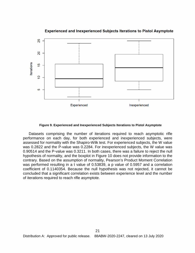
Figure 9. Experienced and Inexperienced Subjects Iterations to Pistol Asymptote
Datasets comprising the number of iterations required to reach asymptotic rifle performance on each day, for both experienced and inexperienced subjects, were assessed for normality with the Shapiro-Wilk test. For experienced subjects, the W value was 0.2822 and the P-value was 0.2284. For inexperienced subjects, the W value was 0.90514 and the P-value was 0.3211. In both cases, there was a failure to reject the null hypothesis of normality, and the boxplot in Figure 10 does not provide information to the contrary. Based on the assumption of normality, Pearson’s Product Moment Correlation was performed resulting in a t value of 0.53839, a p value of 0.5957 and a correlation coefficient of 0.1140354. Because the null hypothesis was not rejected, it cannot be concluded that a significant correlation exists between experience level and the number of iterations required to reach rifle asymptote.

22 Distribution A: Approved for public release. 88ABW-2020-2247, cleared on 13 July 2020
Figure 10. Experienced and Inexperienced Subjects Iterations to Rifle Asymptote 4.1.1.2 Hypothesis 2: Iterations to Reach Asymptote Will Decrease Over Time
As Table 1 indicates, the null hypothesis of a normal distribution was not rejected for any days. The boxplot in Figure 11 is not, however, indicative of a normal distribution. When Bartlett’s Test was performed, the resulting K2 was 1.5517 and the p-value was 0.6704, which failed to reject the null hypothesis of homoscedasticity. The Kruskal-Wallis test yielded a Χ2 value of 1.2683 and a p-value of 0.7367, which failed to reject the null hypothesis of equality of dataset location. Because the null hypothesis was rejected, there is no evidence of any change in the number of iterations required to achieve asymptotic performance with the M9 over 4 days of data collection. Therefore, it cannot be concluded that the number of iterations required to achieve asymptotic performance with the M9 has decreased.
Table 1. Iterations to Reach Pistol Asymptote Shapiro-Wilk Test Results Day W P-value
2 0.93559 0.62389 3 0.91989 0.50454 4 0.89534 0.34713 5 0.81029 0.07259

23 Distribution A: Approved for public release. 88ABW-2020-2247, cleared on 13 July 2020
Figure 11. Pistol Iterations to Asymptote
As Table 2 indicates, the null hypothesis of a normal distribution was not rejected for any days. The boxplot in Figure 12 is not, however, indicative of a normal distribution. A closer examination of the boxplot shows that the Day 4 dataset has a much smaller interquartile range with two outliers. This was not caused by lost data or computational error and is only a reflection of the data collected on that day. When Bartlett’s Test was performed, the resulting K2 was 9.0481 and the p-value was 0.02866, which rejected the null hypothesis of homoscedasticity. The Brunner-Dette-Munk test yielded an F value of 1.095642 and a p-value of 0.37161, which failed to reject the null hypothesis of equality of distribution functions. Because the null hypothesis was not rejected, there is no evidence of a change in the number of iterations required to achieve asymptotic performance with the M4A1 over 4 days of data collection. Therefore, it cannot be concluded that the number of iterations required to achieve asymptotic performance with the M4A1 has decreased.

24 Distribution A: Approved for public release. 88ABW-2020-2247, cleared on 13 July 2020
Table 2. Iterations to Reach Rifle Asymptote Shapiro-Wilk Test Results Day W P-value
2 0.90016 0.37489 3 0.947 0.71593 4 0.92409 0.53531 5 0.87271 0.23722
Figure 12. Rifle Iterations to Asymptote
4.1.1.3 Hypothesis 3: Iterations to Reach Asymptote Differ Significantly for Pistol and Rifle
As Table 3 indicates, the null hypothesis of a normal distribution was not rejected for any days. The boxplot in Figure 13 is not, however, indicative of a normal distribution. When Bartlett’s Test was performed, the resulting K2 was 10.683 and the p-value was 0.153, which failed to reject the null hypothesis of homoscedasticity. The Kruskal-Wallis test yielded a Χ2 value of 4.0455 and a p-value of 0.7745, which failed to reject the null hypothesis of equality of dataset medians. Because the null hypothesis was not rejected, there is no evidence indicative of a significant difference between the number of iterations required to achieve asymptotic performance with the M9 and M4A1.
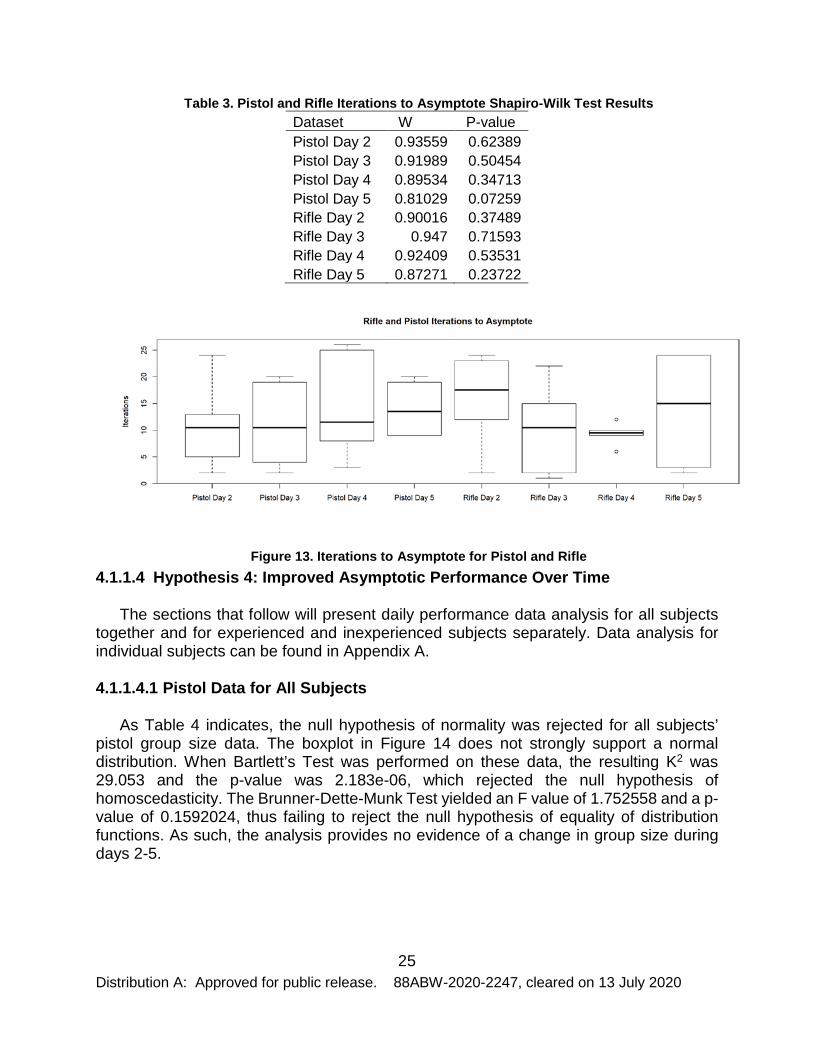
25 Distribution A: Approved for public release. 88ABW-2020-2247, cleared on 13 July 2020
Table 3. Pistol and Rifle Iterations to Asymptote Shapiro-Wilk Test Results Dataset W P-value Pistol Day 2 0.93559 0.62389 Pistol Day 3 0.91989 0.50454 Pistol Day 4 0.89534 0.34713 Pistol Day 5 0.81029 0.07259 Rifle Day 2 0.90016 0.37489 Rifle Day 3 0.947 0.71593 Rifle Day 4 0.92409 0.53531 Rifle Day 5 0.87271 0.23722
Figure 13. Iterations to Asymptote for Pistol and Rifle 4.1.1.4 Hypothesis 4: Improved Asymptotic Performance Over Time
The sections that follow will present daily performance data analysis for all subjects together and for experienced and inexperienced subjects separately. Data analysis for individual subjects can be found in Appendix A.
4.1.1.4.1 Pistol Data for All Subjects
As Table 4 indicates, the null hypothesis of normality was rejected for all subjects’ pistol group size data. The boxplot in Figure 14 does not strongly support a normal distribution. When Bartlett’s Test was performed on these data, the resulting K2 was 29.053 and the p-value was 2.183e-06, which rejected the null hypothesis of homoscedasticity. The Brunner-Dette-Munk Test yielded an F value of 1.752558 and a p-value of 0.1592024, thus failing to reject the null hypothesis of equality of distribution functions. As such, the analysis provides no evidence of a change in group size during days 2-5.

26 Distribution A: Approved for public release. 88ABW-2020-2247, cleared on 13 July 2020
Table 4. All Subjects Pistol Group Size Shapiro-Wilk Test Results Day W P-Value
2 0.79662 3.76E-06 3 0.93475 0.0188 4 0.91268 0.003527 5 0.88292 0.000461
Figure 14. Pistol Group Size for All Subjects
As Table 5 indicates, the null hypothesis of normality was rejected for all subjects’ pistol MPI to CZP distance data. The boxplot in Figure 15 does not strongly support a normal distribution. When Bartlett’s Test was performed on these data, the resulting K2 was 11.542 and the p-value was 0.009129, which rejected the null hypothesis of homoscedasticity. The Brunner-Dette-Munk Test yielded an F value of 1.545646 and a p-value of 0.205295, thus failing to reject the null hypothesis of equality of distribution functions. As such, the analysis provides no evidence of a change in MPI to CZP distance during days 2-5.

27 Distribution A: Approved for public release. 88ABW-2020-2247, cleared on 13 July 2020
Table 5. All Subjects Pistol MPI to CZP Distance Shapiro-Wilk Test Results Day W P-Value
2 0.87741 0.000325 3 0.91425 0.003954 4 0.88482 0.000521 5 0.94701 0.05051
Figure 15. Pistol MPI to CZP Distance for All Subjects
As Table 6 indicates, the null hypothesis of normality was rejected for all subjects’ pistol DCMS data. The boxplot in Figure 16 does not strongly support a normal distribution. When Bartlett’s Test was performed on these data, the resulting K2 was 17.504 and the p-value was 0.0005565, which rejected the null hypothesis of homoscedasticity. The Brunner-Dette-Munk Test yielded an F value of 1.912974 and a p-value of 0.1305129, thus failing to reject the null hypothesis of equality of distribution functions. As such, the analysis provides no evidence of a change in DCMS during days 2-5.

28 Distribution A: Approved for public release. 88ABW-2020-2247, cleared on 13 July 2020
Table 6. All Pistol Subjects DCMS Shapiro-Wilk Test Results Day W P-Value
2 0.84205 3.99E-05 3 0.93378 0.01741 4 0.86399 0.000142 5 0.93562 0.02014
Figure 16. Pistol DCMS for all Subjects
As Table 7 indicates, the null hypothesis of normality was rejected for all subjects’ pistol mean radius data. The boxplot in Figure 17 does not strongly support a normal distribution. When Bartlett’s Test was performed on these data, the resulting K2 was 20.514 and the p-value was 0.0001328, which rejected the null hypothesis of homoscedasticity. The Brunner-Dette-Munk Test yielded an F value of 1.667709 and a p-value of 0.1768368, thus failing to reject the null hypothesis of equality of distribution functions. As such, the analysis provides no evidence of a change in mean radius during days 2-5.

29 Distribution A: Approved for public release. 88ABW-2020-2247, cleared on 13 July 2020
Table 7. All Subjects Pistol Mean Radius Shapiro-Wilk Test Results Day W P-Value
2 0.83763 3.12E-05 3 0.92717 0.01041 4 0.88819 0.00065 5 0.85113 6.67E-05
Figure 17. Pistol Mean Radius Data for All Subjects
4.1.1.4.2 Rifle Data for All Subjects
As Table 8 indicates, the null hypothesis of normality was rejected for days 4 and 5 of all subjects’ rifle group size data. The boxplot in Figure 18 does not strongly support a normal distribution. When Bartlett’s Test was performed on these data, the resulting K2 was 13.069 and the p-value was 0.004489, which rejected the null hypothesis of homoscedasticity. The Brunner-Dette-Munk Test yielded an F value of 1.069877 and a p-value of 0.3630315, thus failing to reject the null hypothesis of equality of distribution functions. As such, the analysis provides no evidence of a change in group size during days 2-5.

30 Distribution A: Approved for public release. 88ABW-2020-2247, cleared on 13 July 2020
Table 8. All Subjects Rifle Group Size Shapiro-Wilk Test Results Day W P-Value
2 0.97743 0.564 3 0.97697 0.5472 4 0.92054 0.006298 5 0.94075 0.03034
Figure 18. Rifle Group Size Data for All Subjects
As Table 9 indicates, the null hypothesis of normality was rejected for day 3 all subjects’ MPI to CZP Distance data. The boxplot in Figure 19 does not strongly support a normal distribution. When Bartlett’s Test was performed on these data, the resulting K2 was 10.432 and the p-value was 0.01523, which rejected the null hypothesis of homoscedasticity. The Brunner-Dette-Munk Test yielded an F value of 0.790427 and a p-value of 0.4976514, thus failing to reject the null hypothesis of equality of distribution functions. As such, the analysis provides no evidence of a change in MPI to CZP distance during days 2-5.

31 Distribution A: Approved for public release. 88ABW-2020-2247, cleared on 13 July 2020
Table 9. All Subjects Rifle MPI to CZP Distance Shapiro-Wilk Test Results Day W P-Value
2 0.97527 0.4875 3 0.87729 0.000322 4 0.9568 0.1133 5 0.97969 0.6495
Figure 19. Rifle MPI to CZP Distance Data for All Subjects
As Table 10 indicates, the null hypothesis of normality was rejected for day 2 of all subjects’ rifle DCMS data. The boxplot in Figure 20 does not strongly support a normal distribution. When Bartlett’s Test was performed on these data, the resulting K2 was 7.5169 and the p-value was 0.05713, which failed to reject the null hypothesis of homoscedasticity. The Kruskal-Wallis Test yielded a Χ2 value of 3.1981 and a p-value of 0.3621, thus failing to reject the null hypothesis of equality of dataset medians. As such, the analysis provides no evidence of a change in DCMS during days 2-5.

32 Distribution A: Approved for public release. 88ABW-2020-2247, cleared on 13 July 2020
Table 10. All Subjects Rifle DCMS Shapiro-Wilk Test Results Day W P-Value
2 0.95101 0.07022 3 0.83626 2.90E-05 4 0.9816 0.7361 5 0.98257 0.7601
Figure 20. Rifle DCMS Data for All Subjects
As Table 11 indicates, the null hypothesis of normality was rejected for days 4 and 5 of all subjects’ rifle mean radius data. The boxplot in Figure 21 does not strongly support a normal distribution. When Bartlett’s Test was performed on these data, the resulting K2 was 11.447 and the p-value was 0.009538, which rejected the null hypothesis of homoscedasticity. The Brunner-Dette-Munk test yielded an F value of 1.662118 and a p-value of 0.1791376, thus failing to reject the null hypothesis of equality of distribution functions. As such, the analysis provides no evidence of change in mean radius during days 2-5.

33 Distribution A: Approved for public release. 88ABW-2020-2247, cleared on 13 July 2020
Table 11. All Subjects Rifle Mean Radius Shapiro-Wilk Test Results Day W P-Value
2 0.98344 0.7926 3 0.97779 0.5775 4 0.90713 0.00271 5 0.92074 0.006393
Figure 21. Rifle Mean Radius Data for All Subjects
4.1.1.4.3 Pistol Data for Experienced Subjects
As Table 12 indicates, the null hypothesis of normality was rejected for days 4 and 5. The boxplot in Figure 22 does not provide information to the contrary. When Bartlett’s Test was performed on these data, the resulting K2 was 2.9197 and the p-value was 0.4042, which failed to reject the null hypothesis of homoscedasticity. The Kruskal-Wallis test yielded a Χ2 value of 5.919 and a p-value of 0.1156, thus failing to reject the null hypothesis of equality of dataset medians. As such, the analysis provides no evidence of a change in group size during days 2-5.

34 Distribution A: Approved for public release. 88ABW-2020-2247, cleared on 13 July 2020
Table 12. Experienced Subjects Pistol Group Size Shapiro-Wilk Test Results Day W P-Value
2 0.9751557 0.7927767 3 0.96484 0.5430018 4 0.9166054 0.0491648 5 0.8466614 0.0018966
Figure 22. Experienced Subjects Pistol Group Size
As Table 13 indicates, the null hypothesis of normality was rejected for days 3 and 4. The boxplot in Figure 23 does not provide information to the contrary. When Bartlett’s Test was performed on these data, the resulting K2 was 2.4336 and the p-value was 0.4874, which failed to reject the null hypothesis of homoscedasticity. The Kruskal-Wallis test yielded a Χ2 value of 9.8918 and a p-value of 0.01951, rejecting the null hypothesis of equality of dataset medians. As Table 14 shows, the only significant differences are between days 3 and 4 and days 4 and 5. These differences are not, however, indicative of a trend because they are not progressive in nature.

35 Distribution A: Approved for public release. 88ABW-2020-2247, cleared on 13 July 2020
Table 13. Experienced Subjects Pistol MPI to CZP Distance Shapiro-Wilk Test Results Day W P-Value
2 0.9255554 0.0775822 3 0.883796 0.0099173 4 0.8876942 0.0119141 5 0.9262214 0.0802784
Figure 23. Experienced Subjects Pistol MPI to CZP Distance Table 14. Experienced Subjects Pistol MPI to CZP Distance Dunn's Test Results
Days Z P-Value 2 & 3 1.19173 0.11668 2 & 4 -1.8705 0.03071 2 & 5 0.26425 0.39579 3 & 4 -3.06224 0.0011 3 & 5 -0.92748 0.17684 4 & 5 2.13476 0.01639
As Table 15 indicates, the null hypothesis of normality was rejected for days 4 and 5. The boxplot in Figure 24 does not provide information to the contrary. When Bartlett’s Test was performed on these data, the resulting K2 was 1.5108 and the p-value was 0.6798, which failed to reject the null hypothesis of homoscedasticity. The Kruskal-Wallis

36 Distribution A: Approved for public release. 88ABW-2020-2247, cleared on 13 July 2020
test yielded a Χ2 value of 6.638 and a p-value of 0.08438, failing to reject the null hypothesis of equality of dataset medians. As such, the analysis does not provide evidence of a change in DCMS during days 2-5.
Table 15. Experienced Subjects Pistol DCMS Shapiro-Wilk Test Results Day W P-Value
2 0.9701117 0.6697473 3 0.9784591 0.8658544 4 0.8256095 0.0007965 5 0.9104593 0.0360888
Figure 24. Experienced Subjects Pistol DCMS
As Table 16 indicates, the null hypothesis of normality was rejected for days 4 and 5. The boxplot in Figure 25 does not provide information to the contrary. When Bartlett’s Test was performed on these data, the resulting K2 was 3.7943 and the p-value was 0.2847, which failed to reject the null hypothesis of homoscedasticity. The Kruskal-Wallis test yielded a Χ2 value of 5.5405 and a p-value of 0.1362, failing to reject the null hypothesis of equality of dataset medians. As such, the analysis does not provide evidence of a change in mean radius during days 2-5.

37 Distribution A: Approved for public release. 88ABW-2020-2247, cleared on 13 July 2020
Table 16. Experienced Subjects Pistol Mean Radius Shapiro-Wilk Test Results Day W P-Value
2 0.9681227 0.6209021 3 0.9796195 0.88875 4 0.9097156 0.0347727 5 0.8336741 0.0011043
Figure 25. Experienced Subjects Pistol Mean Radius
4.1.1.4.4 Pistol Data for Inexperienced Subjects
As Table 17 indicates, the null hypothesis of normality was rejected for days 2 and 3. The boxplot in Figure 26 does not provide information to the contrary. When Bartlett’s Test was performed on these data, the resulting K2 was 10.479 and the p-value was 0.0149, which rejected the null hypothesis of homoscedasticity. The Brunner-Dette-Munk test yielded an F value of 3.402117 and a p-value of 0.02814133, rejecting the null hypothesis of equality of distribution functions. Despite this rejection of the null hypothesis, the REGWQ test failed to reject the null hypothesis for any of its pairwise comparisons. There is therefore no evidence of statistically significant differences. As such, the analysis provides no evidence of a change in group size during days 2-5.
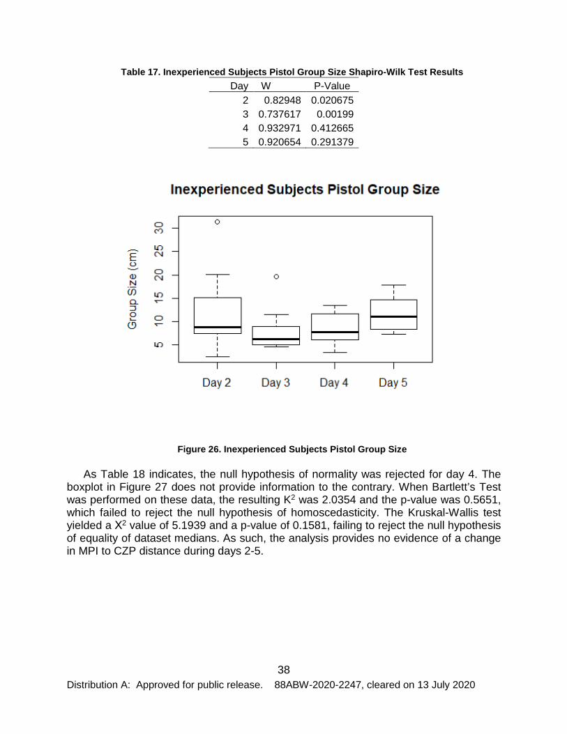
38 Distribution A: Approved for public release. 88ABW-2020-2247, cleared on 13 July 2020
Table 17. Inexperienced Subjects Pistol Group Size Shapiro-Wilk Test Results Day W P-Value
2 0.82948 0.020675 3 0.737617 0.00199 4 0.932971 0.412665 5 0.920654 0.291379
Figure 26. Inexperienced Subjects Pistol Group Size
As Table 18 indicates, the null hypothesis of normality was rejected for day 4. The boxplot in Figure 27 does not provide information to the contrary. When Bartlett’s Test was performed on these data, the resulting K2 was 2.0354 and the p-value was 0.5651, which failed to reject the null hypothesis of homoscedasticity. The Kruskal-Wallis test yielded a Χ2 value of 5.1939 and a p-value of 0.1581, failing to reject the null hypothesis of equality of dataset medians. As such, the analysis provides no evidence of a change in MPI to CZP distance during days 2-5.

39 Distribution A: Approved for public release. 88ABW-2020-2247, cleared on 13 July 2020
Table 18. Inexperienced Subjects Pistol MPI to CZP Distance Shapiro-Wilk Test Results Day W P-Value
2 0.917713 0.267537 3 0.931357 0.394723 4 0.745672 0.002409 5 0.922575 0.307967
Figure 27. Inexperienced Subjects Pistol MPI to CZP Distance
As Table 19 indicates, the null hypothesis of normality was rejected for day 4. The boxplot in Figure 28 does not provide information to the contrary. When Bartlett’s Test was performed on these data, the resulting K2 was 3.8412 and the p-value was 0.2791, which failed to reject the null hypothesis of homoscedasticity. The Kruskal-Wallis test yielded a Χ2 value of 4.7713 and a p-value of 0.1893, failing to reject the null hypothesis of equality of dataset medians. As such, the analysis provides no evidence of a change in DCMS during days 2-5.

40 Distribution A: Approved for public release. 88ABW-2020-2247, cleared on 13 July 2020
Table 19. Inexperienced Subjects Pistol DCMS Shapiro-Wilk Test Results Day W P-Value
2 0.919963 0.285604 3 0.899037 0.154142 4 0.831262 0.021716 5 0.92411 0.321824
Figure 28. Inexperienced Subjects Pistol DCMS
As Table 20 indicates, the null hypothesis of normality was rejected for days 2 and 3. The boxplot in Figure 29 does not provide information to the contrary. When Bartlett’s Test was performed on these data, the resulting K2 was 6.2437 and the p-value was 0.1003, which failed to reject the null hypothesis of homoscedasticity. The Kruskal-Wallis test yielded a Χ2 value of 7.1403 and a p-value of 0.06756, failing to reject the null hypothesis of equality of dataset medians. As such, the analysis provides no evidence of a change in mean radius during days 2-5.
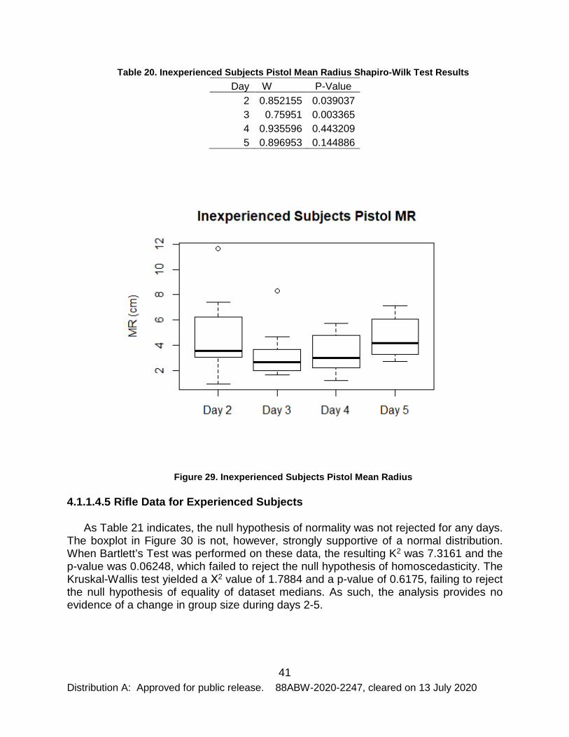
41 Distribution A: Approved for public release. 88ABW-2020-2247, cleared on 13 July 2020
Table 20. Inexperienced Subjects Pistol Mean Radius Shapiro-Wilk Test Results Day W P-Value
2 0.852155 0.039037 3 0.75951 0.003365 4 0.935596 0.443209 5 0.896953 0.144886
Figure 29. Inexperienced Subjects Pistol Mean Radius
4.1.1.4.5 Rifle Data for Experienced Subjects
As Table 21 indicates, the null hypothesis of normality was not rejected for any days. The boxplot in Figure 30 is not, however, strongly supportive of a normal distribution. When Bartlett’s Test was performed on these data, the resulting K2 was 7.3161 and the p-value was 0.06248, which failed to reject the null hypothesis of homoscedasticity. The Kruskal-Wallis test yielded a Χ2 value of 1.7884 and a p-value of 0.6175, failing to reject the null hypothesis of equality of dataset medians. As such, the analysis provides no evidence of a change in group size during days 2-5.

42 Distribution A: Approved for public release. 88ABW-2020-2247, cleared on 13 July 2020
Table 21. Experienced Subjects Rifle Group Size Shapiro-Wilk Test Results Day W P-Value
2 0.9713224 0.6996952 3 0.9713297 0.6998757 4 0.9704841 0.6789547 5 0.9772814 0.8409726
Figure 30. Experienced Subjects Rifle Group Size
As Table 22 indicates, the null hypothesis of normality was rejected for day 3. The boxplot in Figure 31 does not provide information to the contrary. When Bartlett’s Test was performed on these data, the resulting K2 was 10.127 and the p-value was 0.01751, which rejected the null hypothesis of homoscedasticity. The Brunner-Dette-Munk test yielded an F value of 1.589893 and a p-value of 0.1985974, failing to reject the null hypothesis of equality of distribution functions. As such, the analysis provides no evidence of a change in MPI to CZP distance during days 2-5.

43 Distribution A: Approved for public release. 88ABW-2020-2247, cleared on 13 July 2020
Table 22. Experienced Subjects Rifle MPI to CZP Distance Shapiro-Wilk Test Results Day W P-Value
2 0.9534984 0.3220215 3 0.8162298 0.0005493 4 0.9725273 0.7294149 5 0.9771882 0.8389415
Figure 31. Experienced Subjects Rifle MPI to CZP Distance
As Table 23 indicates, the null hypothesis of normality was rejected for days 2 and 3. The boxplot in Figure 32 does not provide information to the contrary. When Bartlett’s Test was performed on these data, the resulting K2 was 9.7794 and the p-value was 0.02054, which rejected the null hypothesis of homoscedasticity. The Brunner-Dette-Munk test yielded an F value of 1.50276 and a p-value of 0.2195349, failing to reject the null hypothesis of equality of distribution functions. As such, the analysis provides no evidence of a change in DCMS during days 2-5.

44 Distribution A: Approved for public release. 88ABW-2020-2247, cleared on 13 July 2020
Table 23. Experienced Subjects Rifle DCMS Shapiro-Wilk Test Results Day W P-Value
2 0.8356841 0.0011993 3 0.7680956 0.0000926 4 0.9694445 0.6532832 5 0.9722728 0.7231561
Figure 32. Experienced Subjects Rifle DCMS
As Table 24 indicates, the null hypothesis of normality was not rejected for any days. The boxplot in Figure 33 does not provide information to the contrary. When Bartlett’s Test was performed on these data, the resulting K2 was 7.7411 and the p-value was 0.05168, which failed to reject the null hypothesis of homoscedasticity. When an ANOVA was performed, the resulting F value was 0.265 and the p-value was 0.851, which failed to reject the null hypothesis of equality of dataset means. As the graph in Figure 34 shows, however, the ANOVA residuals exhibit some deviation from normality in the top quantiles. Since normally distributed residuals are an assumption required for ANOVA, the Kruskal-Wallis test was performed, yielding a Χ2 value of 0.83988 and a p-value of 0.8399, failing to reject the null hypothesis of equality of dataset medians. As such, the analysis provides no evidence of a change in mean radius during days 2-5.

45 Distribution A: Approved for public release. 88ABW-2020-2247, cleared on 13 July 2020
Table 24. Experienced Subjects Rifle Mean Radius Shapiro-Wilk Test Results Day W P-Value
2 0.9702943 0.6742597 3 0.9759051 0.8101756 4 0.978982 0.876385 5 0.9801422 0.8984698
Figure 33. Experienced Subjects Rifle Mean Radius
46 Distribution A: Approved for public release. 88ABW-2020-2247, cleared on 13 July 2020
Figure 34. Experienced Subjects Rifle MR ANOVA Residuals QQ Plot
4.1.1.4.6 Rifle Data for Inexperienced Subjects
As Table 25 indicates, the null hypothesis of normality was not rejected for any days. The boxplot in Figure 35 is not, however, indicative of a normal distribution. When Bartlett’s Test was performed on these data, the resulting K2 was 8.3773 and the p-value was 0.003882, which rejected the null hypothesis of homoscedasticity. The Brunner-Dette-Munk test yielded an F value of 2.508499 and a p-value of 0.0737523, failing to reject the null hypothesis of equality of distribution functions. As such, the analysis provides no evidence of a change in group size during days 2-5.
Table 25. Inexperienced Subjects Rifle Group Size Shapiro-Wilk Test Results Day W P-Value
2 0.926821 0.347626 3 0.908272 0.202728 4 0.943159 0.540047 5 0.936879 0.458725

47 Distribution A: Approved for public release. 88ABW-2020-2247, cleared on 13 July 2020
Figure 35. Inexperienced Subjects Rifle Group Size
As Table 26 indicates, the null hypothesis of normality was not rejected for any days. The boxplot in Figure 36 is not, however, indicative of a normal distribution. When Bartlett’s Test was performed on these data, the resulting K2 was 4.3878 and the p-value was 0.2225, which failed to reject the null hypothesis of homoscedasticity. The Kruskal-Wallis test yielded an F value of 1.2764 and a p-value of 0.7348, failing to reject the null hypothesis of equality of dataset medians. As such, the analysis provides no evidence of a change in MPI to CZP distance during days 2-5.
Table 26. Inexperienced Subjects Rifle MPI to CZP Distance Shapiro-Wilk Test Results Day W P-Value
2 0.940044 0.498641 3 0.884976 0.101531 4 0.864742 0.056075 5 0.942258 0.527872

48 Distribution A: Approved for public release. 88ABW-2020-2247, cleared on 13 July 2020
Figure 36. Inexperienced Subjects Rifle MPI to CZP Distance
As Table 27 indicates, the null hypothesis of normality was not rejected for any days. The boxplot in Figure 37 is not, however, indicative of a normal distribution. When Bartlett’s Test was performed on these data, the resulting K2 was 5.0823 and the p-value was 0.1659, which failed to reject the null hypothesis of homoscedasticity. The Kruskal-Wallis test yielded a Χ2 value of 5.0354 and a p-value of 0.1348, failing to reject the null hypothesis of equality of dataset medians. As such, the analysis provides no evidence of a change in DCMS during days 2-5.
Table 27. Inexperienced Subjects Rifle DCMS Shapiro-Wilk Test Results Day W P-Value
2 0.952379 0.67198 3 0.914546 0.24388 4 0.963411 0.83119 5 0.912813 0.23178

49 Distribution A: Approved for public release. 88ABW-2020-2247, cleared on 13 July 2020
Figure 37. Inexperienced Subjects Rifle DCMS
As Table 28 indicates, the null hypothesis of normality was not rejected for any days. The boxplot in Figure 38 is not, however, indicative of a normal distribution. When Bartlett’s Test was performed on these data, the resulting K2 was 8.9485 and the p-value was 0.02998, which rejected the null hypothesis of homoscedasticity. The Brunner-Dette-Munk test yielded an F value of 4.798265 and a p-value of 0.006580139, rejecting the null hypothesis of equality of distribution functions. As Table 29 shows, the only significant differences were between days 2 and 5 and days 4 and 5. These differences are not, however, indicative of a trend because they are not progressive in nature.
Table 28. Inexperienced Subjects Rifle Mean Radius Shapiro-Wilk Test Results Day W P-Value
2 0.931077 0.391672 3 0.976702 0.966993 4 0.97 0.910807 5 0.950791 0.648578

50 Distribution A: Approved for public release. 88ABW-2020-2247, cleared on 13 July 2020
Figure 38. Inexperienced Subjects Rifle Mean Radius Table 29. Inexperienced Subjects Rifle Mean Radius REGWQ Test Results
Days Statistic Adj. P-Values CI 2 & 3 2.1855 0.1294 0.9864 2 & 4 1.1894 0.4049 0.5368 2 & 5 3.58 0.0391 1.6158 3 & 4 3.3749 0.0547 1.5232 3 & 5 1.3945 0.3295 0.6294 4 & 5 4.7694 0.0082 2.1526
4.1.1.4.7 Experienced and Inexperienced Pistol Data Comparison
As Table 30 indicates, the null hypothesis of normality was rejected for experienced subjects on days 4 and 5 and for inexperienced subjects on days 2 and 3. The boxplot in Figure 39 does not provide information to the contrary. When Bartlett’s Test was performed on these data, the resulting K2 was 30.68 and the p-value was 7.122e-05, which rejected the null hypothesis of homoscedasticity. The Brunner-Dette-Munk test yielded an F value of 3.325502 and a p-value of 0.005955575, rejecting the null hypothesis of equality of distribution functions.

51 Distribution A: Approved for public release. 88ABW-2020-2247, cleared on 13 July 2020
Table 30. Experienced and Inexperienced Subjects Pistol Group Size Shapiro-Wilk Test Results
Dataset W P-Value Exp. Day 2 0.97516 0.79278 Inexp. Day 2 0.82948 0.02067 Exp. Day 3 0.96484 0.543 Inexp. Day 3 0.73762 0.00199 Exp. Day 4 0.91661 0.04916 Inexp. Day 4 0.93297 0.41266 Exp. Day 5 0.84666 0.0019 Inexp. Day 5 0.92065 0.29138
Figure 39. Experienced and Inexperienced Subjects Pistol Group Size
As Table 31 indicates, there were statistically significant differences between experienced and inexperienced subjects only on day 5.
Table 31. Experienced and Inexperienced Subjects Pistol Group Size REGWQ Test Results Day Statistic Adj. P-Value CI
2 3.2142 0.0631 3.0679 3 0.3548 0.8023 0.3387 4 0.9492 0.9078 0.906 5 4.6675 0.0206 4.455
As Table 32 indicates, the null hypothesis of normality was rejected for experienced subjects on days 3 and 4 and for inexperienced subjects on days 4 and 5. The boxplot in Figure 40 does not provide information to the contrary. When Bartlett’s Test was performed on these data, the resulting K2 was 13.73 and the p-value was 0.05619, which failed to reject the null hypothesis of homoscedasticity. The Kruskal-Wallis test yielded a Χ2 value of 21.727 and a p-value of 0.0002831 rejecting the null hypothesis of equality of dataset medians. While this null hypothesis was rejected, the results of Dunn’s test in Table 33 indicate that there were significant differences between experienced and inexperienced subjects only on days 2 and 3.
52 Distribution A: Approved for public release. 88ABW-2020-2247, cleared on 13 July 2020
Table 32. Experienced and Inexperienced Subjects Pistol MPI to CZP Distance Shapiro-Wilk Test Results
Dataset W P-Value Exp. Day 2 0.92556 0.07758 Inexp. Day 2 0.91771 0.26754 Exp. Day 3 0.8838 0.00992 Inexp. Day 3 0.93136 0.39472 Exp. Day 4 0.88769 0.01191 Inexp. Day 4 0.74567 0.00241 Exp. Day 5 0.92622 0.08028 Inexp. Day 5 0.74567 0.00241
Figure 40. Experienced and Inexperienced Subjects Pistol MPI to CZP Distance Table 33. Experienced and Inexperienced Subjects Pistol MPI to CZP Distance Dunn's Test
Results Days Z P-Value
2 -2.7179 0.0033 3 -2.814 0.0024 4 0.45487 0.3246 5 -0.5425 0.2938
As Table 34 indicates, the null hypothesis of normality was rejected for experienced subjects on days 4 and 5 and for inexperienced subjects on day 4. The boxplot in Figure 41 does not provide information to the contrary. When Bartlett’s Test was performed on these data, the resulting K2 was 19.723 and the p-value was 0.001408, which rejected the null hypothesis of homoscedasticity. The Brunner-Dette-Munk test yielded an F value of 1.995968 and a p-value of 0.106942 failing to reject the null hypothesis of equality of distribution functions. As such, the analysis provides no evidence of a change in DCMS during days 2-5.

53 Distribution A: Approved for public release. 88ABW-2020-2247, cleared on 13 July 2020
Table 34. Experienced and Inexperienced Subjects Pistol DCMS Shapiro-Wilk Test Results Dataset W P-Value Exp. Day 2 0.97011 0.66975 Inexp. Day 2 0.91996 0.2856 Exp. Day 3 0.97846 0.86585 Inexp. Day 3 0.89904 0.15414 Exp. Day 4 0.82561 0.0008 Inexp. Day 4 0.83126 0.02172 Exp. Day 5 0.91046 0.03609 Inexp. Day 5 0.92411 0.32182
Figure 41. Experienced and Inexperienced Subjects Pistol DCMS
As Table 35 indicates, the null hypothesis of normality was rejected for experienced subjects on days 4 and 5 and for inexperienced subjects on days 2 and 3. The boxplot in Figure 42 does not provide information to the contrary. When Bartlett’s Test was performed on these data, the resulting K2 was 27.578 and the p-value was 0.0002622, which rejected the null hypothesis of homoscedasticity. The Brunner-Dette-Munk test yielded an F value of 2.868689 and a p-value of 0.01472509 rejecting the null hypothesis of equality of distribution functions. While this null hypothesis was rejected, the results of the REGWQ test in Table 36 indicate that significant differences between experienced and inexperienced subjects were present only on day 5.

54 Distribution A: Approved for public release. 88ABW-2020-2247, cleared on 13 July 2020
Table 35. Experienced and Inexperienced Subjects Pistol Mean Radius Shapiro-Wilk Test Results
Dataset W P-Value Exp. Day 2 0.96812 0.6209 Inexp. Day 2 0.85216 0.03904 Exp. Day 3 0.97962 0.88875 Inexp. Day 3 0.75951 0.00336 Exp. Day 4 0.90972 0.03477 Inexp. Day 4 0.9356 0.44321 Exp. Day 5 0.83367 0.0011 Inexp. Day 5 0.89695 0.14489
Figure 42. Experienced and Inexperienced Subjects Pistol Mean Radius Table 36. Experienced and Inexperienced Subjects Pistol Mean Radius REGWQ Test Results
Day Statistic P-Value CI 2 2.9779 0.0924 1.126 3 0.0963 0.9458 0.0364 4 0.9062 0.9186 0.3426 5 4.5458 0.0266 1.7188
4.1.1.4.8 Experienced and Inexperienced Rifle Data Comparison
As Table 37 indicates, the null hypothesis of normality was not rejected for experienced or inexperienced subjects on any days. The boxplot in Figure 43 is not, however, indicative of a normal distribution. When Bartlett’s Test was performed on these data, the resulting K2 was 22.999 and the p-value was 0.001705, which rejected the null hypothesis of homoscedasticity. The Brunner-Dette-Munk test yielded an F value of 1.970595 and a p-value of 0.08144472 failing to reject the null hypothesis of equality of distribution functions. As such, the analysis provides no evidence of a change in group size during days 2-5.
55 Distribution A: Approved for public release. 88ABW-2020-2247, cleared on 13 July 2020
Table 37. Experienced and Inexperienced Subjects Rifle Group Size Shapiro-Wilk Test Results Dataset W P-Value Exp. Day 2 0.9713224 0.6997 Inexp. Day 2 0.9268205 0.34763 Exp. Day 3 0.9713297 0.69988 Inexp. Day 3 0.9082719 0.20273 Exp. Day 4 0.9704841 0.67895 Inexp. Day 4 0.9431590 0.54005 Exp. Day 5 0.9772814 0.84097 Inexp. Day 5 0.9368787 0.45873
Figure 43. Experienced and Inexperienced Subjects Rifle Group Size
As Table 38 indicates, the null hypothesis of normality was rejected for experienced subjects on days 4 and 5 and for inexperienced subjects on days 2 and 3. The boxplot in Figure 44 does not provide information to the contrary. When Bartlett’s Test was performed on these data, the resulting K2 was 14.888 and the p-value was 0.03746, which rejected the null hypothesis of homoscedasticity. The Brunner-Dette-Munk test yielded an F value of 0.7060654 and a p-value of 0.6359203 failing to reject the null hypothesis of equality of distribution functions. As such, the analysis provides no evidence of a change in MPI to CZP distance during days 2-5.

56 Distribution A: Approved for public release. 88ABW-2020-2247, cleared on 13 July 2020
Table 38. Experienced and Inexperienced Subjects Rifle MPI to CZP Distance Shapiro-Wilk Test Results
Dataset W P-Value Exp. Day 2 0.9751557 0.79278 Inexp. Day 2 0.8294795 0.02067 Exp. Day 3 0.9648400 0.543 Inexp. Day 3 0.7376168 0.00199 Exp. Day 4 0.9166054 0.04916 Inexp. Day 4 0.9329706 0.41266 Exp. Day 5 0.8466614 0.0019 Inexp. Day 5 0.9206544 0.29138
Figure 44. Experienced and Inexperienced Subjects Rifle MPI to CZP Distance
As Table 39 indicates, the null hypothesis of normality was rejected for experienced subjects on days 2 and 3. The boxplot in Figure 45 does not provide information to the contrary. When Bartlett’s Test was performed on these data, the resulting K2 was 15.092 and the p-value was 0.03484, which rejected the null hypothesis of homoscedasticity. The Brunner-Dette-Munk test yielded an F value of 1.607432 and a p-value of 0.1569926 failing to reject the null hypothesis of equality of distribution functions. As such, the analysis provides no evidence of a change in DCMS during days 2-5.

57 Distribution A: Approved for public release. 88ABW-2020-2247, cleared on 13 July 2020
Table 39. Experienced and Inexperienced Subjects Rifle DCMS Shapiro-Wilk Test Results Dataset W P-Value Exp. Day 2 0.8356841 0.0012 Inexp. Day 2 0.9523788 0.67198 Exp. Day 3 0.7680956 9.3E-05 Inexp. Day 3 0.9145457 0.24388 Exp. Day 4 0.9694445 0.65328 Inexp. Day 4 0.9634113 0.83119 Exp. Day 5 0.9722728 0.72316 Inexp. Day 5 0.9128128 0.23178
Figure 45. Experienced and Inexperienced Subjects Rifle DCMS
As Table 40 indicates, the null hypothesis of normality was not rejected for any subjects on any days. The boxplot in Figure 46 is not, however, indicative of a normal distribution. When Bartlett’s Test was performed on these data, the resulting K2 was 25.538 and the p-value was 0.0006089, which rejected the null hypothesis of homoscedasticity. The Brunner-Dette-Munk test yielded an F value of 3.14643 and a p-value of 0.007721839 rejecting the null hypothesis of equality of distribution functions. While this null hypothesis was rejected, the results of the REGWQ test in Table 41 indicate that significant differences between experienced and inexperienced subjects were present only on day 4.

58 Distribution A: Approved for public release. 88ABW-2020-2247, cleared on 13 July 2020
Table 40. Experienced and Inexperienced Subjects Rifle Mean Radius Shapiro-Wilk Test Results
Dataset W P-Value Exp. Day 2 0.9702943 0.67426 Inexp. Day 2 0.9310774 0.39167 Exp. Day 3 0.9759051 0.81018 Inexp. Day 3 0.9767017 0.96699 Exp. Day 4 0.9789820 0.87639 Inexp. Day 4 0.9700003 0.91081 Exp. Day 5 0.9801422 0.89847 Inexp. Day 5 0.9507910 0.64858
Figure 46. Experienced and Inexperienced Subjects Rifle Mean Radius Table 41. Experienced and Inexperienced Subjects Rifle Mean Radius REGWQ Test Results
Day Statistic Adj. P-Value CI 2 3.2857 0.0978 1.0293 3 0.2555 0.8569 0.08 4 5.324 0.0033 1.6678 5 1.4778 0.2979 0.4629
4.1.2 Marksmanship Speed-Accuracy Experiment
In this experiment, the hypothesis tested was that the level of asymptotic performance will improve to a small, but significant, extent over time. In the sections that follow, the analyzed data used to test this hypothesis are presented for both all subjects combined. Data analysis for individual subjects can be found in Appendix B.
4.1.2.1 IES Scoring Results
The MPI to CZP distance based IES results shown in Figure 47 are indicative of similar trends for radii of 5 and 4 cm. The trend for 3 cm was similar to those trends, but was greater in amplitude on days 4 and 5.
59 Distribution A: Approved for public release. 88ABW-2020-2247, cleared on 13 July 2020
Figure 47. All Subjects IES - MPI to CZP Distance Based
The MPI to CZP distance based RT results in Figure 48 show very similar trends for all radii, with no extreme changes. The amplitude of each curve, however, is different, with the 5 cm curve having the largest amplitude and the 2 cm curve having the smallest. This result is unexpected, as accurate shots at a smaller sized target would be expected to require more time.
Figure 48. All Subjects RT - MPI to CZP Distance Based
MPI to CZP distance based proportion correct results, illustrated in Figure 49, show
0
20
40
60
80
100
120
Day 2 Day 3 Day 4 Day 5
IES
All Subjects IES - MPI to CZP Distance Based
5 cm
4 cm
3 cm
2 cm
0
1
2
3
4
5
6
7
Day 2 Day 3 Day 4 Day 5
RT (s
)
All Subjects RT - MPI to CZP Distance Based
5 cm
4 cm
3 cm
2 cm

60 Distribution A: Approved for public release. 88ABW-2020-2247, cleared on 13 July 2020
more hits at greater radii, although the hit proportions for the 5 cm and 4 cm radii on day 3 are relatively close, due to the significant decrease in the 5 cm results. Overall, the trend among all radii was a decrease from day 2 to day 5.
Figure 49. All Subjects Proportion Correct - MPI to CZP Distance Based
The DCMS based IES results, illustrated in Figure 50, show nearly identical trends for radii of 5 and 4 cm. The 3 cm results show an increase from day 2 to day 3 and greater overall values. The 2 cm results are greater overall and show an extreme increase from day 2 to day 3, followed by large decreases.
0
0.1
0.2
0.3
0.4
0.5
0.6
0.7
0.8
Day 2 Day 3 Day 4 Day 5
Prop
ortio
n Co
rrec
t
All Subjects Proportion Correct - MPI to CZP Distance Based
5 cm
4 cm
3 cm
2 cm

61 Distribution A: Approved for public release. 88ABW-2020-2247, cleared on 13 July 2020
Figure 50. All Subjects IES - DCMS Based The DCMS based RT results illustrated in Figure 51 show trends similar to those of
the MPI to CZP distance based RT results, with the curves having a similar shape and the unexpected result of larger RT values being associated with larger radii.
Figure 51. All Subjects RT - DCMS Based
The DCMS based proportion correct results illustrated in Figure 52 show patterns similar to those of the MPI to CZP distance based results, with greater radii having greater overall proportions correct. Additionally, the 2 and 3 cm radii curves showed decreases from day 2 to day 3.
0
10
20
30
40
50
60
70
Day 2 Day 3 Day 4 Day 5
DCM
S
All Subjects IES - DCMS Based
5 cm
4 cm
3 cm
2 cm
0
1
2
3
4
5
6
Day 2 Day 3 Day 4 Day 5
RT (s
)
All Subjects RT - DCMS Based
5 cm
4 cm
3 cm
2 cm

62 Distribution A: Approved for public release. 88ABW-2020-2247, cleared on 13 July 2020
Figure 52. All Subjects Proportion Correct - DCMS Based 4.1.2.2 Conditional Accuracy Function Results
As Table 42 indicates, the null hypothesis of a normal distribution was rejected for all quantiles. The boxplot in Figure 53 does not provide information to the contrary. Bartlett’s test produced a K2 value of 12.94 and a p value of 0.01157, rejecting the null hypothesis of homoscedasticity. The Brunner-Dette-Munk test produced an F value of 0.1432361 and a p value of 0.9642724, failing to reject the null hypothesis of equality of distribution functions. Because this null hypothesis was not rejected, it cannot be concluded that accuracy, as measured by 1/MPI to CZP distance, differed by time quantile on day 2.
Table 42. All Subjects Day 2 Five Quantile 1/MPI to CZP Distance Shapiro-Wilk Test Results Quantile W P-Value
1 0.90448 0.02681 2 0.83262 0.00106 3 0.81975 0.00063 4 0.87244 0.00588 5 0.77883 0.00014
0
0.1
0.2
0.3
0.4
0.5
0.6
0.7
0.8
Day 2 Day 3 Day 4 Day 5
Prop
ortio
n Co
rrec
t
All Subjects Proportion Correct - DCMS Based
5 cm
4 cm
3 cm
2 cm
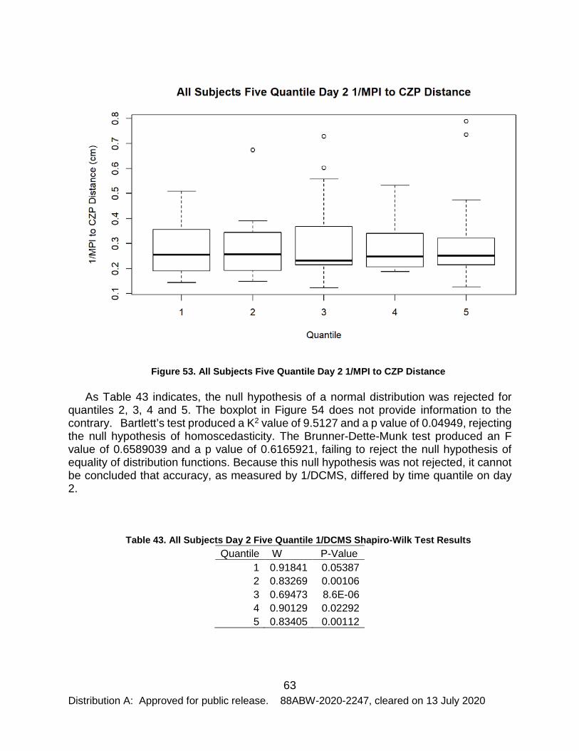
63 Distribution A: Approved for public release. 88ABW-2020-2247, cleared on 13 July 2020
Figure 53. All Subjects Five Quantile Day 2 1/MPI to CZP Distance
As Table 43 indicates, the null hypothesis of a normal distribution was rejected for quantiles 2, 3, 4 and 5. The boxplot in Figure 54 does not provide information to the contrary. Bartlett’s test produced a K2 value of 9.5127 and a p value of 0.04949, rejecting the null hypothesis of homoscedasticity. The Brunner-Dette-Munk test produced an F value of 0.6589039 and a p value of 0.6165921, failing to reject the null hypothesis of equality of distribution functions. Because this null hypothesis was not rejected, it cannot be concluded that accuracy, as measured by 1/DCMS, differed by time quantile on day 2.
Table 43. All Subjects Day 2 Five Quantile 1/DCMS Shapiro-Wilk Test Results Quantile W P-Value
1 0.91841 0.05387 2 0.83269 0.00106 3 0.69473 8.6E-06 4 0.90129 0.02292 5 0.83405 0.00112

64 Distribution A: Approved for public release. 88ABW-2020-2247, cleared on 13 July 2020
Figure 54. All Subjects Five Quantile Day 2 1/DCMS As Table 44 indicates, the null hypothesis of a normal distribution was rejected for all
quantiles. The boxplot in Figure 55 does not provide information to the contrary. Bartlett’s test produced a K2 value of 62.746, and a p value of 7.676e-13, rejecting the null hypothesis of homoscedasticity. The Brunner-Dette-Munk test produced an F value of 0.8241289 and a p value of 0.5081353, failing to reject the null hypothesis of equality of distribution functions. Because this null hypothesis was not rejected, it cannot be concluded that accuracy, as measured by 1/MPI to CZP distance, differed by time quantile on day 3.
Table 44. All Subjects Day 3 Five Quantile 1/MPI to CZP Distance Shapiro-Wilk Test Results
Quantile W P-Value 1 0.6485 2.30E-06 2 0.68261 6.00E-06 3 0.76645 8.75E-05 4 0.60452 7.00E-07 5 0.69618 1.25E-05
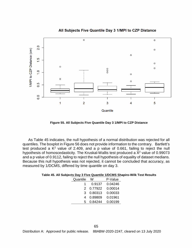
65 Distribution A: Approved for public release. 88ABW-2020-2247, cleared on 13 July 2020
Figure 55. All Subjects Five Quantile Day 3 1/MPI to CZP Distance
As Table 45 indicates, the null hypothesis of a normal distribution was rejected for all quantiles. The boxplot in Figure 56 does not provide information to the contrary. Bartlett’s test produced a K2 value of 2.409, and a p value of 0.661, failing to reject the null hypothesis of homoscedasticity. The Kruskal-Wallis test produced a Χ2 value of 0.99073 and a p value of 0.9112, failing to reject the null hypothesis of equality of dataset medians. Because this null hypothesis was not rejected, it cannot be concluded that accuracy, as measured by 1/DCMS, differed by time quantile on day 3.
Table 45. All Subjects Day 3 Five Quantile 1/DCMS Shapiro-Wilk Test Results
Quantile W P-Value 1 0.9137 0.04246 2 0.77922 0.00014 3 0.80313 0.00033 4 0.89809 0.01961 5 0.84244 0.00199

66 Distribution A: Approved for public release. 88ABW-2020-2247, cleared on 13 July 2020
Figure 56. All Subjects Five Quantile Day 3 1/DCMS As Table 46 indicates, the null hypothesis of a normal distribution was rejected for
quantiles 2, 4 and 5. The boxplot in Figure 57 does not provide information to the contrary. Bartlett’s test produced a K2 value of 93.523, and a p value of 2.2e-16, rejecting the null hypothesis of homoscedasticity. The Brunner-Dette-Munk test produced an F value of 0.589869 and a p value of 0.6673954, failing to reject the null hypothesis of equality of distribution functions. Because this null hypothesis was not rejected, it cannot be concluded that accuracy, as measured by 1/MPI to CZP distance, differed by time quantile on day 4.
Table 46. All Subjects Day 4 Five Quantile 1/MPI to CZP Distance Shapiro-Wilk Test Results
Quantile W P-Value 1 0.93201 0.10812 2 0.90101 0.02261 3 0.9413 0.17434 4 0.52151 1E-07 5 0.62581 1.2E-06

67 Distribution A: Approved for public release. 88ABW-2020-2247, cleared on 13 July 2020
Figure 57. All Subjects Five Quantile Day 41/MPI to CZP Distance As Table 47 indicates, the null hypothesis of a normal distribution was rejected for
quantile 1. The boxplot in Figure 58 does not provide information to the contrary. Bartlett’s test produced a K2 value of 11.469, and a p value of 0.02177, rejecting the null hypothesis of homoscedasticity. The Brunner-Dette-Munk test produced an F value of 1.100987 and a p value of 0.3593446, failing to reject the null hypothesis of equality of distribution functions. Because this null hypothesis was not rejected, it cannot be concluded that accuracy, as measured by 1/DCMS, differed by time quantile on day 4.
Table 47. All Subjects Day 4 Five Quantile 1/DCMS Shapiro-Wilk Test Results
Quantile W P-Value 1 0.81437 0.00051 2 0.92716 0.08425 3 0.94521 0.21285 4 0.97598 0.81193 5 0.92895 0.09234

68 Distribution A: Approved for public release. 88ABW-2020-2247, cleared on 13 July 2020
Figure 58. All Subjects Five Quantile Day 4 1/DCMS As Table 48 indicates, the null hypothesis of a normal distribution was rejected for
quantile 4. The boxplot in Figure 59 does not provide information to the contrary. Bartlett’s test produced a K2 value of 9.8443, and a p value of 0.04313, rejecting the null hypothesis of homoscedasticity. The Brunner-Dette-Munk test produced an F value of 0.5221038 and a p value of 0.7190319, failing to reject the null hypothesis of equality of distribution functions. Because this null hypothesis was not rejected, it cannot be concluded that accuracy, as measured by 1/MPI to CZP distance, differed by time quantile on day 5.
Table 48. All Subjects Day 5 Five Quantile 1/MPI to CZP Distance Shapiro-Wilk Test Results
Quantile W P-Value 1 0.93149 0.10527 2 0.9557 0.35821 3 0.92185 0.06417 4 0.73381 2.9E-05 5 0.92926 0.09383

69 Distribution A: Approved for public release. 88ABW-2020-2247, cleared on 13 July 2020
Figure 59. All Subjects Five Quantile Day 5 1/MPI to CZP Distance As Table 49 indicates, the null hypothesis of a normal distribution was rejected for
quantiles 1, 2, 3 and 5. The boxplot in Figure 60 does not provide information to the contrary. Bartlett’s test produced a K2 value of 7.5399, and a p value of 0.11, failing to reject the null hypothesis of homoscedasticity. The Kruskal-Wallis test produced a Χ2 value of 11.139 and a p value of 0.02504, rejecting the null hypothesis of equality of dataset medians. Because this null hypothesis was rejected, it can be concluded that accuracy, as measured by 1/DCMS, differed by time quantile on day 5. As Table 50 indicates, differences were found between quantiles 1 and 4 and 5 and quantiles 3 and 4 and 5.
Table 49. All Subjects Day 5 Five Quantile 1/DCMS Shapiro-Wilk Test Results
Quantile W P-Value 1 0.88662 0.01133 2 0.83541 0.00119 3 0.80791 0.0004 4 0.94908 0.2588 5 0.8594 0.00328

70 Distribution A: Approved for public release. 88ABW-2020-2247, cleared on 13 July 2020
Figure 60. All Subjects Five Quantile Day 5 1/DCMS
Table 50. All Subjects Five Quantile Day 5 1/DCMS Distance Dunn’s Test Results Quantiles Z P-Value 1 & 2 -0.83818 0.201 1 & 3 0.07054 0.4719 1 & 4 -2.4938 0.0063 1 & 5 -2.0913 0.0183 2 & 3 0.90872 0.1817 2 & 4 -1.65562 0.0489 2 & 5 -1.25312 0.1051 3 & 4 -2.56434 0.0052 3 & 5 -2.16184 0.0153 4 & 5 0.40249 0.3437
As Table 51 indicates, the null hypothesis of a normal distribution was rejected for
quantiles 2, 3, 4, 5 and 6. The boxplot in Figure 61 does not provide information to the contrary. Bartlett’s test produced a K2 value of 8.8693, and a p value of 0.1144, failing to reject the null hypothesis of homoscedasticity. The Kruskal-Wallis test produced a Χ2 value of 1.5771 and a p value of 0.904, rejecting the null hypothesis of equality of dataset medians. Because this null hypothesis was not rejected, it cannot be concluded that accuracy, as measured by 1/MPI to CZP distance, differed by time quantile on day 2.

71 Distribution A: Approved for public release. 88ABW-2020-2247, cleared on 13 July 2020
Table 51. All Subjects Day 2 Six Quantile 1/MPI to CZP Distance Shapiro-Wilk Test Results Quantile W P-Value
1 0.91455 0.07786 2 0.81386 0.0014 3 0.79268 0.00067 4 0.79073 0.00063 5 0.89508 0.03338 6 0.75182 0.00018
Figure 61. All Subjects Six Quantile Day 2 1/MPI to CZP Distance As Table 52 indicates, the null hypothesis of a normal distribution was rejected for
quantiles 3, 4, 5 and 6. The boxplot in Figure 62 does not provide information to the contrary. Bartlett’s test produced a K2 value of 21.669, and a p value of 0.0006052, rejecting the null hypothesis of homoscedasticity. The Brunner-Dette-Munk test produced an F value of 0.6613966 and a p value of 0.6464815, failing to reject the null hypothesis of equality of distribution functions. Because this null hypothesis was not rejected, it cannot be concluded that accuracy, as measured by 1/DCMS, differed by time quantile on day 2.

72 Distribution A: Approved for public release. 88ABW-2020-2247, cleared on 13 July 2020
Table 52. All Subjects Day 2 Six Quantile 1/DCMS Shapiro-Wilk Test Results Quantile W P-Value
1 0.91378 0.07525 2 0.93683 0.20879 3 0.75231 0.00018 4 0.84797 0.00493 5 0.86068 0.00809 6 0.86795 0.01082
Figure 62. All Subjects Six Quantile Day 2 1/DCMS
As Table 53 indicates, the null hypothesis of a normal distribution was rejected for all quantiles. The boxplot in Figure 63 does not provide information to the contrary. Bartlett’s test produced a K2 value of 68.843, and a p value of 1.784e-13, rejecting the null hypothesis of homoscedasticity. The Brunner-Dette-Munk test produced an F value of 0.4942797 and a p value of 0.7733031, failing to reject the null hypothesis of equality of distribution functions. Because this null hypothesis was not rejected, it cannot be concluded that accuracy, as measured by 1/MPI to CZP distance, differed by time quantile on day 3.
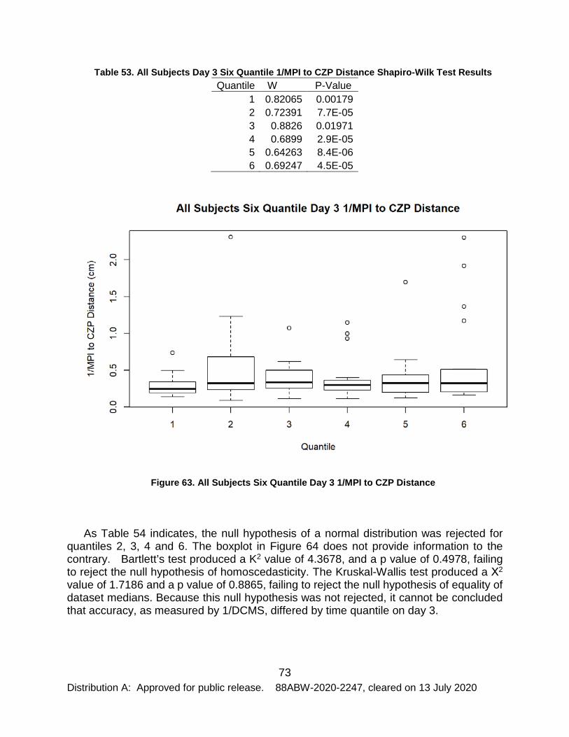
73 Distribution A: Approved for public release. 88ABW-2020-2247, cleared on 13 July 2020
Table 53. All Subjects Day 3 Six Quantile 1/MPI to CZP Distance Shapiro-Wilk Test Results Quantile W P-Value
1 0.82065 0.00179 2 0.72391 7.7E-05 3 0.8826 0.01971 4 0.6899 2.9E-05 5 0.64263 8.4E-06 6 0.69247 4.5E-05
Figure 63. All Subjects Six Quantile Day 3 1/MPI to CZP Distance
As Table 54 indicates, the null hypothesis of a normal distribution was rejected for quantiles 2, 3, 4 and 6. The boxplot in Figure 64 does not provide information to the contrary. Bartlett’s test produced a K2 value of 4.3678, and a p value of 0.4978, failing to reject the null hypothesis of homoscedasticity. The Kruskal-Wallis test produced a Χ2 value of 1.7186 and a p value of 0.8865, failing to reject the null hypothesis of equality of dataset medians. Because this null hypothesis was not rejected, it cannot be concluded that accuracy, as measured by 1/DCMS, differed by time quantile on day 3.

74 Distribution A: Approved for public release. 88ABW-2020-2247, cleared on 13 July 2020
Table 54. All Subjects Day 3 Six Quantile 1/DCMS Shapiro-Wilk Test Results Quantile W P-Value
1 0.91008 0.06395 2 0.83327 0.00283 3 0.82343 0.00197 4 0.72446 7.9E-05 5 0.9304 0.15717 6 0.86478 0.01178
Figure 64. All Subjects Six Quantile Day 3 1/DCMS
As Table 55 indicates, the null hypothesis of a normal distribution was rejected for quantiles 3, 5, and 6. The boxplot in Figure 65 does not provide information to the contrary. Bartlett’s test produced a K2 value of 105.82, and a p value of 2.2e-16, rejecting the null hypothesis of homoscedasticity. The Brunner-Dette-Munk test produced an F value of 0.3614712 and a p value of 0.8711046, failing to reject the null hypothesis of equality of distribution functions. Because this null hypothesis was not rejected, it cannot be concluded that accuracy, as measured by 1/MPI to CZP distance, differed by time quantile on day 4.

75 Distribution A: Approved for public release. 88ABW-2020-2247, cleared on 13 July 2020
Table 55. All Subjects Day 4 Six Quantile 1/MPI to CZP Distance Shapiro-Wilk Test Results Quantile W P-Value
1 0.94203 0.26181 2 0.95983 0.54046 3 0.8908 0.02782 4 0.98927 0.99712 5 0.50129 3E-07 6 0.66824 1.6E-05
Figure 65. All Subjects Six Quantile Day 41/MPI to CZP Distance
As Table 56 indicates, the null hypothesis of a normal distribution was rejected for quantiles 2, 3, 4, and 6. The boxplot in Figure 66 does not provide information to the contrary. Bartlett’s test produced a K2 value of 12.856, and a p value of 0.02476, rejecting the null hypothesis of homoscedasticity. The Brunner-Dette-Munk test produced an F value of 1.364962 and a p value of 0.2432773, failing to reject the null hypothesis of equality of distribution functions. Because this null hypothesis was not rejected, it cannot be concluded that accuracy, as measured by 1/DCMS, differed by time quantile on day 4.

76 Distribution A: Approved for public release. 88ABW-2020-2247, cleared on 13 July 2020
Table 56. All Subjects Day 4 Six Quantile 1/DCMS Shapiro-Wilk Test Results Quantile W P-Value
1 0.91008 0.06395 2 0.83327 0.00283 3 0.82343 0.00197 4 0.72446 7.9E-05 5 0.9304 0.15717 6 0.86478 0.01178
Figure 66. All Subjects Six Quantile Day 4 1/DCMS
As Table 57 indicates, the null hypothesis of a normal distribution was rejected for quantile 5. The boxplot in Figure 67 does not provide information to the contrary. Bartlett’s test produced a K2 value of 11.223, and a p value of 0.04713, rejecting the null hypothesis of homoscedasticity. The Brunner-Dette-Munk test produced an F value of 0.3310675 and a p value of 0.8919332, failing to reject the null hypothesis of equality of distribution functions. Because this null hypothesis was not rejected, it cannot be concluded that accuracy, as measured by 1/MPI to CZP distance, differed by time quantile on day 5.

77 Distribution A: Approved for public release. 88ABW-2020-2247, cleared on 13 July 2020
Table 57. All Subjects Day 5 Six Quantile 1/MPI to CZP Distance Shapiro-Wilk Test Results Quantile W P-Value
1 0.94481 0.29512 2 0.92467 0.1219 3 0.9274 0.13759 4 0.92383 0.11743 5 0.67357 1.9E-05 6 0.95022 0.37049
Figure 67. All Subjects Six Quantile Day 5 1/MPI to CZP Distance
As Table 58 indicates, the null hypothesis of a normal distribution was rejected for quantiles 1, 2, 3 and 6. The boxplot in Figure 68 does not provide information to the contrary. Bartlett’s test produced a K2 value of 18.119, and a p value of 0.002801, rejecting the null hypothesis of homoscedasticity. The Brunner-Dette-Munk test produced an F value of 1.441457 and a p value of 0.2179119, failing to reject the null hypothesis of equality of distribution functions. Because this null hypothesis was not rejected, it cannot be concluded that accuracy, as measured by 1/DCMS, differed by time quantile on day 5.
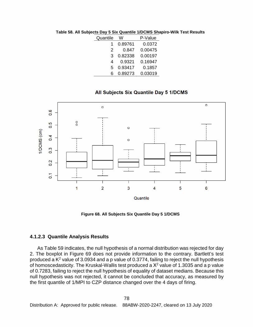
78 Distribution A: Approved for public release. 88ABW-2020-2247, cleared on 13 July 2020
Table 58. All Subjects Day 5 Six Quantile 1/DCMS Shapiro-Wilk Test Results Quantile W P-Value
1 0.89761 0.0372 2 0.847 0.00475 3 0.82338 0.00197 4 0.9321 0.16947 5 0.93417 0.1857 6 0.89273 0.03019
Figure 68. All Subjects Six Quantile Day 5 1/DCMS
4.1.2.3 Quantile Analysis Results
As Table 59 indicates, the null hypothesis of a normal distribution was rejected for day 2. The boxplot in Figure 69 does not provide information to the contrary. Bartlett’s test produced a K2 value of 3.0934 and a p value of 0.3774, failing to reject the null hypothesis of homoscedasticity. The Kruskal-Wallis test produced a Χ2 value of 1.3035 and a p value of 0.7283, failing to reject the null hypothesis of equality of dataset medians. Because this null hypothesis was not rejected, it cannot be concluded that accuracy, as measured by the first quantile of 1/MPI to CZP distance changed over the 4 days of firing.

79 Distribution A: Approved for public release. 88ABW-2020-2247, cleared on 13 July 2020
Table 59. All Subjects Quantile 1 of 5 1/MPI to CZP Distance Shapiro-Wilk Test Results Day W P-Value
2 0.90448 0.02681 3 0.92021 0.05904 4 0.95868 0.41249 5 0.93149 0.10527
Figure 69. All Subjects Quantile 1 of 5 1/MPI to CZP Distance
As Table 60 indicates, the null hypothesis of a normal distribution was rejected for days 2 and 3. The boxplot in Figure 70 does not provide information to the contrary. Bartlett’s test produced a K2 value of 46.056 and a p value of 5.517e-10, rejecting the null hypothesis of homoscedasticity. The Brunner-Dette-Munk test produced an F value of 0.4992092 and a p value of 0.6689532 failing to reject the null hypothesis of equality of distribution functions. Because this null hypothesis was not rejected, it cannot be concluded that accuracy, as measured by the second quantile of 1/MPI to CZP distance changed over the 4 days of firing.
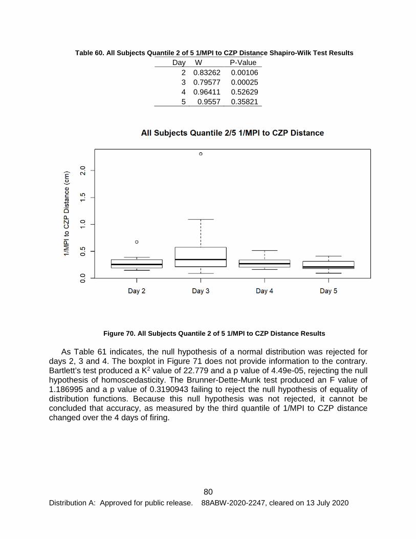
80 Distribution A: Approved for public release. 88ABW-2020-2247, cleared on 13 July 2020
Table 60. All Subjects Quantile 2 of 5 1/MPI to CZP Distance Shapiro-Wilk Test Results Day W P-Value
2 0.83262 0.00106 3 0.79577 0.00025 4 0.96411 0.52629 5 0.9557 0.35821
Figure 70. All Subjects Quantile 2 of 5 1/MPI to CZP Distance Results
As Table 61 indicates, the null hypothesis of a normal distribution was rejected for days 2, 3 and 4. The boxplot in Figure 71 does not provide information to the contrary. Bartlett’s test produced a K2 value of 22.779 and a p value of 4.49e-05, rejecting the null hypothesis of homoscedasticity. The Brunner-Dette-Munk test produced an F value of 1.186995 and a p value of 0.3190943 failing to reject the null hypothesis of equality of distribution functions. Because this null hypothesis was not rejected, it cannot be concluded that accuracy, as measured by the third quantile of 1/MPI to CZP distance changed over the 4 days of firing.

81 Distribution A: Approved for public release. 88ABW-2020-2247, cleared on 13 July 2020
Table 61. All Subjects Quantile 3 of 5 1/MPI to CZP Distance Shapiro-Wilk Test Results Day W P-Value
2 0.81975 0.00063 3 0.75963 6.9E-05 4 0.76013 7E-05 5 0.92185 0.06417
Figure 71. All Subjects Quantile 3 of 5 1/MPI to CZP Distance Results
As Table 62 indicates, the null hypothesis of a normal distribution was rejected for all days. The boxplot in Figure 72 does not provide information to the contrary. Bartlett’s test produced a K2 value of 41.275 and a p value of 5.718e-09, rejecting the null hypothesis of homoscedasticity. The Brunner-Dette-Munk test produced an F value of 0.7322615 and a p value of 0.5347482 failing to reject the null hypothesis of equality of distribution functions. Because this null hypothesis was not rejected, it cannot be concluded that accuracy, as measured by the fourth quantile of 1/MPI to CZP distance changed over the 4 days of firing.

82 Distribution A: Approved for public release. 88ABW-2020-2247, cleared on 13 July 2020
Table 62. All Subjects Quantile 4 of 5 1/MPI to CZP Distance Shapiro-Wilk Test Results Day W P-Value
2 0.87244 0.00588 3 0.52941 1E-07 4 0.79729 0.00027 5 0.73381 2.9E-05
Figure 72. All Subjects Quantile 4 of 5 1/MPI to CZP Distance Results
As Table 63 indicates, the null hypothesis of a normal distribution was rejected for days 2, 3 and 4. The boxplot in Figure 73 does not provide information to the contrary. Bartlett’s test produced a K2 value of 86.146 and a p value of 2.2e-16, rejecting the null hypothesis of homoscedasticity. The Brunner-Dette-Munk test produced an F value of 0.860738 and a p value of 0.462061 failing to reject the null hypothesis of equality of distribution functions. Because this null hypothesis was not rejected, it cannot be concluded that accuracy, as measured by the fifth quantile of 1/MPI to CZP distance changed over the 4 days of firing.

83 Distribution A: Approved for public release. 88ABW-2020-2247, cleared on 13 July 2020
Table 63. All Subjects Quantile 5 of 5 1/MPI to CZP Distance Shapiro-Wilk Test Results Day W P-Value
2 0.77883 0.00014 3 0.546 2E-07 4 0.78885 0.00019 5 0.92926 0.09383
Figure 73. All Subjects Quantile 5 of 5 1/MPI to CZP Distance Results
As Table 64 indicates, the null hypothesis of a normal distribution was rejected for days 4 and 5. The boxplot in Figure 74 does not provide information to the contrary. Bartlett’s test produced a K2 value of 2.062 and a p value of 0.5596, failing to reject the null hypothesis of homoscedasticity. The Kruskal-Wallis test produced a Χ2 value of 2.4319 and a p value of 0.4877 failing to reject the null hypothesis of equality of dataset medians. Because this null hypothesis was not rejected, it cannot be concluded that accuracy, as measured by the first quantile of 1/DCMS changed over the 4 days of firing.

84 Distribution A: Approved for public release. 88ABW-2020-2247, cleared on 13 July 2020
Table 64. All Subjects Quantile 1 of 5 1/DCMS Shapiro-Wilk Test Results Day W P-Value
2 0.91841 0.05387 3 0.95246 0.30604 4 0.85214 0.0024 5 0.86047 0.00344
Figure 74. All Subjects Quantile 1 of 5 1/DCMS Results
As Table 65 indicates, the null hypothesis of a normal distribution was rejected for days 2, 3 and 5. The boxplot in Figure 75 does not provide information to the contrary. Bartlett’s test produced a K2 value of 9.0251 and a p value of 0.02896, rejecting the null hypothesis of homoscedasticity. The Brunner-Dette-Munk test produced an F value of 0.3048699 and a p value of 0.8193313 failing to reject the null hypothesis of equality of distribution functions. Because this null hypothesis was not rejected, it cannot be concluded that accuracy, as measured by the second quantile of 1/DCMS changed over the 4 days of firing.

85 Distribution A: Approved for public release. 88ABW-2020-2247, cleared on 13 July 2020
Table 65. All Subjects Quantile 2 of 5 1/DCMS Shapiro-Wilk Test Results Day W P-Value
2 0.83269 0.00106 3 0.82822 0.00088 4 0.93036 0.09931 5 0.83541 0.00119
Figure 75. All Subjects Quantile 2 of 5 1/DCMS Results
As Table 66 indicates, the null hypothesis of a normal distribution was rejected for days 2, 3 and 5. The boxplot in Figure 76 does not provide information to the contrary. Bartlett’s test produced a K2 value of 22.238 and a p value of 5.819e-05, rejecting the null hypothesis of homoscedasticity. The Brunner-Dette-Munk test produced an F value of 0.6551942 and a p value of 0.5801358 failing to reject the null hypothesis of equality of distribution functions. Because this null hypothesis was not rejected, it cannot be concluded that accuracy, as measured by the third quantile of 1/DCMS changed over the 4 days of firing.

86 Distribution A: Approved for public release. 88ABW-2020-2247, cleared on 13 July 2020
Table 66. All Subjects Quantile 3 of 5 1/DCMS Shapiro-Wilk Test Results Day W P-Value
2 0.69473 8.6E-06 3 0.8788 0.00786 4 0.94582 0.21953 5 0.80791 0.0004
Figure 76. All Subjects Quantile 3 of 5 1/DCMS Results
As Table 67 indicates, the null hypothesis of a normal distribution was rejected for day 2. The boxplot in Figure 77 does not provide information to the contrary. Bartlett’s test produced a K2 value of 8.0069 and a p value of 0.04587, rejecting the null hypothesis of homoscedasticity. The Brunner-Dette-Munk test produced an F value of 0.9929416 and a p value of 0.3986247 failing to reject the null hypothesis of equality of distribution functions. Because this null hypothesis was not rejected, it cannot be concluded that accuracy, as measured by the fourth quantile of 1/DCMS changed over the 4 days of firing.

87 Distribution A: Approved for public release. 88ABW-2020-2247, cleared on 13 July 2020
Table 67. All Subjects Quantile 4 of 5 1/DCMS Shapiro-Wilk Test Results Day W P-Value
2 0.90129 0.02292 3 0.92038 0.05953 4 0.97598 0.81193 5 0.94908 0.2588
Figure 77. All Subjects Quantile 4 of 5 1/DCMS Results
As Table 68 indicates, the null hypothesis of a normal distribution was rejected for days 2, 3 and 5. The boxplot in Figure 78 does not provide information to the contrary. Bartlett’s test produced a K2 value of 1.9017 and a p value of 0.593, failing to reject the null hypothesis of homoscedasticity. The Kruskal-Wallis test produced a Χ2 value of 1.5907 and a p value of 0.6615 failing to reject the null hypothesis of equality of dataset medians. Because this null hypothesis was not rejected, it cannot be concluded that accuracy, as measured by the fifth quantile of 1/DCMS changed over the 4 days of firing.

88 Distribution A: Approved for public release. 88ABW-2020-2247, cleared on 13 July 2020
Table 68. All Subjects Quantile 5 of 5 1/DCMS Shapiro-Wilk Test Results Day W P-Value
2 0.83405 0.00112 3 0.78417 0.00022 4 0.93117 0.10351 5 0.8594 0.00328
Figure 78. All Subjects Quantile 5 of 5 1/DCMS Results
As Table 69 indicates, the null hypothesis of a normal distribution was not rejected for any days. The boxplot in Figure 79 is not, however, strongly supportive of a normal distribution. Bartlett’s test produced a K2 value of 2.4733 and a p value of 0.4801, failing to reject the null hypothesis of homoscedasticity. The Kruskal-Wallis test produced a Χ2 value of 1.5208 and a p value of 0.6775 failing to reject the null hypothesis of equality of dataset medians. Because this null hypothesis was not rejected, it cannot be concluded that accuracy, as measured by the first quantile of 1/MPI to CZP distance changed over the 4 days of firing.

89 Distribution A: Approved for public release. 88ABW-2020-2247, cleared on 13 July 2020
Table 69. All Subjects Quantile 1 of 6 1/MPI to CZP Distance Shapiro-Wilk Test Results Day W P-Value
2 0.91455 0.07786 3 0.91789 0.09025 4 0.96494 0.64638 5 0.94481 0.29512
Figure 79. All Subjects Quantile 1 of 6 1/MPI to CZP Distance Results
As Table 70 indicates, the null hypothesis of a normal distribution was rejected for days 2 and 3. The boxplot in Figure 80 does not provide information to the contrary. Bartlett’s test produced a K2 value of 28.779 and a p value of 2.492e-06, rejecting the null hypothesis of homoscedasticity. The Brunner-Dette-Munk test produced an F value of 0.5761924 and a p value of 0.6282732 failing to reject the null hypothesis of equality of distrubiton functions. Because this null hypothesis was not rejected, it cannot be concluded that accuracy, as measured by the second quantile of 1/MPI to CZP distance changed over the 4 days of firing.

90 Distribution A: Approved for public release. 88ABW-2020-2247, cleared on 13 July 2020
Table 70. All Subjects Quantile 2 of 6 1/MPI to CZP Distance Shapiro-Wilk Test Results Day W P-Value
2 0.81386 0.0014 3 0.74961 0.00017 4 0.98496 0.98128 5 0.92467 0.1219
Figure 80. All Subjects Quantile 2 of 6 1/MPI to CZP Distance Results
As Table 71 indicates, the null hypothesis of a normal distribution was rejected for days 2 and 4. The boxplot in Figure 81 does not provide information to the contrary. Bartlett’s test produced a K2 value of 5.3959 and a p value of 0.145, failing to reject the null hypothesis of homoscedasticity. The Kruskal-Wallis test produced a Χ2 value of 2.118 and a p value of 0.5483 failing to reject the null hypothesis of equality of dataset medians. Because this null hypothesis was not rejected, it cannot be concluded that accuracy, as measured by the third quantile of 1/MPI to CZP distance changed over the 4 days of firing.

91 Distribution A: Approved for public release. 88ABW-2020-2247, cleared on 13 July 2020
Table 71. All Subjects Quantile 3 of 6 1/MPI to CZP Distance Shapiro-Wilk Test Results Day W P-Value
2 0.79268 0.00067 3 0.91698 0.08667 4 0.87746 0.01593 5 0.9274 0.13759
Figure 81. All Subjects Quantile 3 of 6 1/MPI to CZP Distance Results
As Table 72 indicates, the null hypothesis of a normal distribution was rejected for days 2, 3 and 4. The boxplot in Figure 82 does not provide information to the contrary. Bartlett’s test produced a K2 value of 22.313 and a p value of 5.614e-05, rejecting the null hypothesis of homoscedasticity. The Brunner-Dette-Munk test produced an F value of 1.00391 and a p value of 0.3955436 failing to reject the null hypothesis of equality of distribution functions. Because this null hypothesis was not rejected, it cannot be concluded that accuracy, as measured by the fourth quantile of 1/MPI to CZP distance changed over the 4 days of firing.

92 Distribution A: Approved for public release. 88ABW-2020-2247, cleared on 13 July 2020
Table 72. All Subjects Quantile 4 of 6 1/MPI to CZP Distance Shapiro-Wilk Test Results Day W P-Value
2 0.79073 0.00063 3 0.6387 7.6E-06 4 0.60746 3.5E-06 5 0.92383 0.11743
Figure 82. All Subjects Quantile 4 of 6 1/MPI to CZP Distance Results
As Table 73 indicates, the null hypothesis of a normal distribution was rejected for days 2, 3 and 4. The boxplot in Figure 83 does not provide information to the contrary. Bartlett’s test produced a K2 value of 36.349 and a p value of 6.317e-08, rejecting the null hypothesis of homoscedasticity. The Brunner-Dette-Munk test produced an F value of 1.198046 and a p value of 0.3161735 failing to reject the null hypothesis of equality of dataset medians. Because this null hypothesis was not rejected, it cannot be concluded that accuracy, as measured by the fifth quantile of 1/MPI to CZP distance changed over the 4 days of firing.

93 Distribution A: Approved for public release. 88ABW-2020-2247, cleared on 13 July 2020
Table 73. All Subjects Quantile 5 of 6 1/MPI to CZP Distance Shapiro-Wilk Test Results Day W P-Value
2 0.89508 0.03338 3 0.62259 5.1E-06 4 0.78324 0.00049 5 0.67357 1.9E-05
Figure 83. All Subjects Quantile 5 of 6 1/MPI to CZP Distance Results
As Table 74 indicates, the null hypothesis of a normal distribution was rejected for days 2, 3 and 4. The boxplot in Figure 84 does not provide information to the contrary. Bartlett’s test produced a K2 value of 73.623 and a p value of 7.149e-16, rejecting the null hypothesis of homoscedasticity. The Brunner-Dette-Munk test produced an F value of 0.3627782 and a p value of 0.778951 failing to reject the null hypothesis of equality of distribution functions. Because this null hypothesis was not rejected, it cannot be concluded that accuracy, as measured by the sixth quantile of 1/MPI to CZP distance changed over the 4 days of firing.

94 Distribution A: Approved for public release. 88ABW-2020-2247, cleared on 13 July 2020
Table 74. All Subjects Quantile 6 of 6 1/MPI to CZP Distance Shapiro-Wilk Test Results Day W P-Value
2 0.75182 0.00018 3 0.53648 1.1E-06 4 0.77581 0.00038 5 0.95022 0.37049
Figure 84. All Subjects Quantile 6 of 6 1/MPI to CZP Distance Results
As Table 75 indicates, the null hypothesis of a normal distribution was rejected for days 3 and 4. The boxplot in Figure 85 does not provide information to the contrary. Bartlett’s test produced a K2 value of 1.8111 and a p value of 0.6125, failing to reject the null hypothesis of homoscedasticity. The Kruskal-Wallis test produced a Χ2 value of 0.62796 and a p value of 0.89 failing to reject the null hypothesis of equality of dataset medians. Because this null hypothesis as not rejected, it cannot be concluded that accuracy, as measured by the first quantile of 1/DCMS changed over the 4 days of firing.

95 Distribution A: Approved for public release. 88ABW-2020-2247, cleared on 13 July 2020
Table 75. All Subjects Quantile 1 of 6 1/DCMS Shapiro-Wilk Test Results Day W P-Value
2 0.91378 0.07525 3 0.94506 0.29827 4 0.81101 0.00127 5 0.89761 0.0372
Figure 85. All Subjects Quantile 1 of 6 1/DCMS Results
As Table 76 indicates, the null hypothesis of a normal distribution was rejected for days 3 and 5. The boxplot in Figure 86 does not provide information to the contrary. Bartlett’s test produced a K2 value of 7.2022 and a p value of 0.06573, failing to reject the null hypothesis of homoscedasticity. The Kruskal-Wallis test produced a Χ2 value of 1.6213 and a p value of 0.6546 failing to reject the null hypothesis of equality of dataset medians. Because this null hypothesis as not rejected, it cannot be concluded that accuracy, as measured by the second quantile of 1/DCMS changed over the 4 days of firing.

96 Distribution A: Approved for public release. 88ABW-2020-2247, cleared on 13 July 2020
Table 76. All Subjects Quantile 2 of 6 1/DCMS Shapiro-Wilk Test Results Day W P-Value
2 0.93683 0.20879 3 0.81569 0.0015 4 0.93448 0.18821 5 0.847 0.00475
Figure 86. All Subjects Quantile 2 of 6 1/DCMS Results
As Table 77 indicates, the null hypothesis of a normal distribution was rejected for days 2, 3 and 5. The boxplot in Figure 87 does not provide information to the contrary. Bartlett’s test produced a K2 value of 33.711 and a p value of 2.28e-07, rejecting the null hypothesis of homoscedasticity. The Brunner-Dette-Munk test produced an F value of 1.6185 and a p value of 0.1934844 failing to reject the null hypothesis of equality of distribution functions. Because this null hypothesis as not rejected, it cannot be concluded that accuracy, as measured by the third quantile of 1/DCMS changed over the 4 days of firing.

97 Distribution A: Approved for public release. 88ABW-2020-2247, cleared on 13 July 2020
Table 77. All Subjects Quantile 3 of 6 1/DCMS Shapiro-Wilk Test Results Day W P-Value
2 0.75231 0.00018 3 0.88554 0.02229 4 0.94534 0.30186 5 0.82338 0.00197
Figure 87. All Subjects Quantile 3 of 6 1/DCMS Results
As Table 78 indicates, the null hypothesis of a normal distribution was rejected for days 2 and 3. The boxplot in Figure 88 does not provide information to the contrary. Bartlett’s test produced a K2 value of 4.6072 and a p value of 0.2029, failing to reject the null hypothesis of homoscedasticity. The Kruskal-Wallis test produced a Χ2 value of 0.46463 and a p value of 0.9266 failing to reject the null hypothesis of equality of dataset medians. Because this null hypothesis as not rejected, it cannot be concluded that accuracy, as measured by the fourth quantile of 1/DCMS changed over the 4 days of firing.

98 Distribution A: Approved for public release. 88ABW-2020-2247, cleared on 13 July 2020
Table 78. All Subjects Quantile 4 of 6 1/DCMS Shapiro-Wilk Test Results Day W P-Value
2 0.84797 0.00493 3 0.78856 0.00059 4 0.96566 0.66183 5 0.9321 0.16947
Figure 88. All Subjects Quantile 4 of 6 1/DCMS Results
As Table 79 indicates, the null hypothesis of a normal distribution was rejected for day 2. The boxplot in Figure 89 does not provide information to the contrary. Bartlett’s test produced a K2 value of 10.619 and a p value of 0.01398, rejecting the null hypothesis of homoscedasticity. The Brunner-Dette-Munk test produced an F value of 0.7840732 and a p value of 0.5028214 failing to reject the null hypothesis of equality of distribution functions. Because this null hypothesis as not rejected, it cannot be concluded that accuracy, as measured by the fifth quantile of 1/DCMS changed over the 4 days of firing.

99 Distribution A: Approved for public release. 88ABW-2020-2247, cleared on 13 July 2020
Table 79. All Subjects Quantile 5 of 6 1/DCMS Shapiro-Wilk Test Results Day W P-Value
2 0.86068 0.00809 3 0.97576 0.86847 4 0.97102 0.77627 5 0.93417 0.1857
Figure 89. All Subjects Quantile 5 of 6 1/DCMS Results
As Table 80 indicates, the null hypothesis of a normal distribution was rejected for days 2, 3 and 5. The boxplot in Figure 90 does not provide information to the contrary. Bartlett’s test produced a K2 value of 2.2302 and a p value of 0.526, failing to reject the null hypothesis of homoscedasticity. The Kruskal-Wallis test produced a Χ2 value of 1.6134 and a p value of 0.6564 failing to reject the null hypothesis of equality of dataset medians. Because this null hypothesis as not rejected, it cannot be concluded that accuracy, as measured by the sixth quantile of 1/DCMS changed over the 4 days of firing.
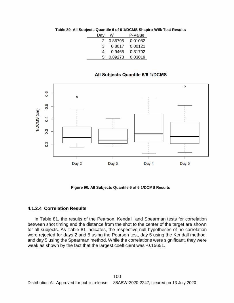
100 Distribution A: Approved for public release. 88ABW-2020-2247, cleared on 13 July 2020
Table 80. All Subjects Quantile 6 of 6 1/DCMS Shapiro-Wilk Test Results Day W P-Value
2 0.86795 0.01082 3 0.8017 0.00121 4 0.9465 0.31702 5 0.89273 0.03019
Figure 90. All Subjects Quantile 6 of 6 1/DCMS Results
4.1.2.4 Correlation Results
In Table 81, the results of the Pearson, Kendall, and Spearman tests for correlation between shot timing and the distance from the shot to the center of the target are shown for all subjects. As Table 81 indicates, the respective null hypotheses of no correlation were rejected for days 2 and 5 using the Pearson test, day 5 using the Kendall method, and day 5 using the Spearman method. While the correlations were significant, they were weak as shown by the fact that the largest coefficient was -0.15651.

101 Distribution A: Approved for public release. 88ABW-2020-2247, cleared on 13 July 2020
Table 81. All Subjects Correlation Results Pearson Kendall Spearman
Day T P-Value Coefficient Z P-Value Tau S P-Value Rho 2 -2.4955 0.01303 -0.1308 -1.5289 0.1263 -0.05415 8396200 0.1309 -0.07976 3 -1.4147 0.158 -0.07487 -0.58189 0.5606 -0.0207 7807300 0.5778 -0.02955 4 0.5758 0.5651 0.030418 1.7879 0.07378 0.063358 7014300 0.0634 0.097943 5 -2.939 0.003507 -0.15349 -2.9114 0.003598 -0.10319 8992900 0.002906 -0.15651
4.1.3 Marksmanship Visual Search Experiment
The analysis presented in this section was performed on the pooled data of all subjects. Individual subject data analyses are available in Appendix C of this document. As indicated in Table 82, the null hypothesis of equality of proportions was not rejected for any of the visual acuities over the 4 days of firing. As indicated in Table 83, performance did not differ to a significant extent at any of the visual acuities on any individual day of firing. Hit proportions and 95% confidence intervals for each acuity over the days of firing are provided in Figures 91-94.
Table 82. Subjects VS01-VS10 Acuity Hit Proportions Acuity Day 2 Day 3 Day 4 Day 5 Chi-Squared P-Value A 0.95938 0.95283 0.95313 0.96386 0.57811 0.9014 B 0.95938 0.95925 0.95938 0.95968 0.00069 1 C 0.94375 0.96238 0.94688 0.95968 1.7439 0.6272 D 0.92813 0.925 0.9375 0.92771 0.43322 0.9333
Table 83. Subjects VS01-VS10 Daily Hit Proportions Day Acuity A Acuity B Acuity C Acuity D Chi-Squared P-Value
2 0.95938 0.95938 0.94375 0.92813 4.3312 0.2279 3 0.94984 0.95925 0.96238 0.925 5.6958 0.1274 4 0.95313 0.95938 0.94688 0.9375 1.7342 0.6294 5 0.96386 0.95968 0.95968 0.92771 4.6755 0.1972

102 Distribution A: Approved for public release. 88ABW-2020-2247, cleared on 13 July 2020
Figure 91. Subjects VS01-VS10 Acuity A Hit Proportions
Figure 92. Subjects VS01-VS10 Acuity B Hit Proportions
0.88
0.9
0.92
0.94
0.96
0.98
1
Hit P
ropo
rtio
ns
Subjects VS01-VS10 Acuity A Hit Proportions with 95% Confidence Intervals
Day 2
Day 3
Day 4
Day 5
0.89
0.9
0.91
0.92
0.93
0.94
0.95
0.96
0.97
0.98
0.99
Hit P
ropo
rtio
ns
Subjects VS01-VS10 Acuity B Hit Proportions with 95% Confidence Intervals
Day 2
Day 3
Day 4
Day 5
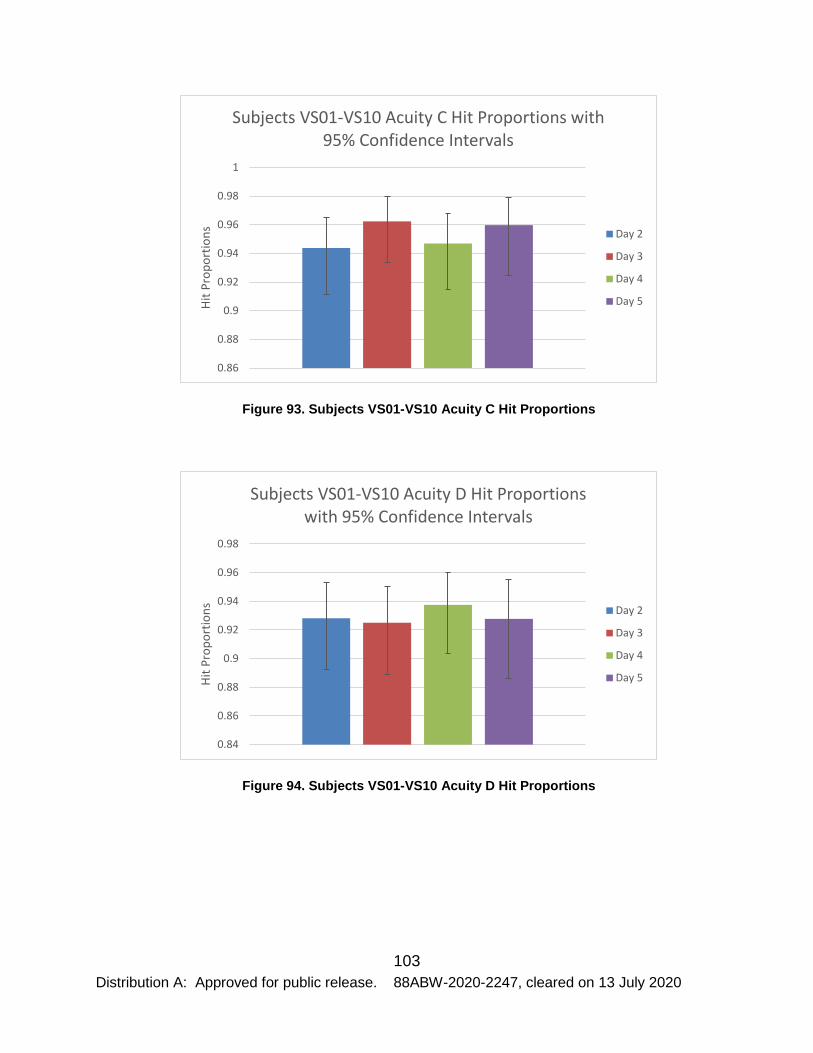
103 Distribution A: Approved for public release. 88ABW-2020-2247, cleared on 13 July 2020
Figure 93. Subjects VS01-VS10 Acuity C Hit Proportions
Figure 94. Subjects VS01-VS10 Acuity D Hit Proportions
0.86
0.88
0.9
0.92
0.94
0.96
0.98
1
Hit P
ropo
rtio
ns
Subjects VS01-VS10 Acuity C Hit Proportions with 95% Confidence Intervals
Day 2
Day 3
Day 4
Day 5
0.84
0.86
0.88
0.9
0.92
0.94
0.96
0.98
Hit P
ropo
rtio
ns
Subjects VS01-VS10 Acuity D Hit Proportions with 95% Confidence Intervals
Day 2
Day 3
Day 4
Day 5

104 Distribution A: Approved for public release. 88ABW-2020-2247, cleared on 13 July 2020
4.2 Discussion 4.2.1 Marksmanship Accuracy and Precision Experiment 4.2.1.1 Hypothesis 1: Experience Level and Iterations to Reach Asymptote
As presented in section 4.1.1.1, there was no significant correlation found between the experience level of the test subjects and the number of iterations required to reach asymptotic performance during each day of firing. One potential issue with the experiment and its results lies with the sample sizes, which were 4 for experienced subjects and 2 for inexperienced subjects. Since such small and disparate sample sizes have the potential to be problematic when using hypothesis tests that compare two samples, data were pooled and tested for a correlation between experience level and the number of iterations to reach asymptote. By pooling the data and performing the analysis in this manner, the total dataset size was 24 days of firing, with 16 experienced days and 8 inexperienced days.
While the failure to reject the null hypothesis of a correlation between the level of test subject experience and the number of iterations required to reach asymptote does not prove the nonexistence of such a correlation, it does not provide any evidence in support of such a relationship. In practical terms, these results imply that the number of iterations in the experimental design was able to accommodate both experienced and inexperienced subjects. As such, the authors see no reason to change the number of iterations in follow on investigations.
4.2.1.2 Hypothesis 2: Iterations to Reach Asymptote Will Decrease Over Time
In the results presented in section 4.1.1.2, the datasets for all subjects were pooled by day and compared for both pistol and rifle. In the case of the pistol data, testing failed to reject the null hypothesis of normality. The boxplot in Figure 11, however, was indicative of potential bias in the data and did not lend strong support to the assumption of normality. Further analysis, via the Kruskal-Wallis test, resulted in a failure to reject the null hypothesis of equality of dataset location. Since the analyses do not provide evidence of any change in dataset location, it cannot be concluded that the number of iterations required to reach pistol asymptote decreased over the four days of data collection. As with the pistol data, the assumption of normality could not be satisfied for the rifle data in section 4.1.1.2. In addition, it was determined that the assumption of homoscedasticity could not be met. As a result, the Brunner-Dette-Munk test was performed, and the null hypothesis of equality of distribution functions was not rejected. Failure to reject this null hypothesis does not provide evidence of a significant change in the distribution functions, to include measures of central tendency and extremes, over the duration of the experiment. Because there is no evidence in support of such changes, it cannot be concluded that the number of iterations required to reach rifle asymptote decreased during the experiment.
For both the pistol and rifle datasets, the failure to reject the respective null hypotheses does not prove that the number of iterations required to reach asymptote did not change,

105 Distribution A: Approved for public release. 88ABW-2020-2247, cleared on 13 July 2020
but it does not provide sufficient evidence to state that there was a change. While these results imply that the number of iterations required to reach asymptote will not significantly change over four days of firing, the principal practical implication is that there is no need to change the present design, as the number of iterations is adequate and not excessive when subjects have a basic level of proficiency.
4.2.1.3 Hypothesis 3: Iterations to Reach Asymptote Differ Significantly for Pistol and Rifle
Several marksmanship practices, such as proper sight alignment and picture and a smooth and controlled trigger squeeze, are common to both pistols and rifles. Significant differences in the weight of the weapon, the grip and the increased stability provided by resting a rifle against the shoulder, however, compelled the investigators to infer that there may be differences in the number of iterations required to reach asymptotic performance with each weapon. In section 4.1.1.3, the results of the analysis of differences in the number of iterations required to reach asymptote with each weapon were presented. While the null hypothesis of normality was not rejected, the boxplot in Figure 13 was indicative of potential bias in the data. Since the null hypothesis of homoscedasticity was not rejected, the Kruskal-Wallis test was performed, resulting a in a failure to reject the null hypothesis of equality of dataset means. Based on the failure to reject this null hypothesis, the investigators do not have evidence to support any assertion that there is a difference in the number of iterations required to reach asymptotic performance with a pistol or rifle under the conditions of the experiments. The practical implication for these results is that the number of iterations is suitable for both weapons and there is therefore no reason to change it for follow on experiments.
4.2.1.4 Hypothesis 4: Improved Asymptotic Performance Over Time
The investigation of the improvement of asymptotic marksmanship performance over time was of particular interest to the investigators, due to the potential for such improvements to mask the effects of treatment with a pilocarpine solution in follow on studies. In section 4.1.1.4, data for all subjects and for experienced and inexperienced subjects were analyzed. The results of this analysis indicated that there were no significant differences between any days for firing for either the rifle or the pistol. When data for experienced and inexperienced subjects were considered separately, there were 3 instances in which significant differences were found between metrics on two or more days of firing. As with the previously discussed results, these results were not indicative of a trend, and no continuous improvement was found for either group with the pistol or the rifle. The practical implications for these results are profound for the design and execution of further marksmanship studies with treatments that include pilocarpine and various combinations of CBRN protective equipment. Since there is no evidence to support the assertion that statistically significant improvements to accuracy and precision in pistol and rifle marksmanship will occur over 4 days of simulated firing, provided the subjects have a basic level of proficiency, future experiments may be designed with one day of firing to collect control data, followed by three days of firing to collect experimental data with one or more treatments. Such experiments would allow for more meaningful

106 Distribution A: Approved for public release. 88ABW-2020-2247, cleared on 13 July 2020
data collection, and analyses such as the combined effects of pilocarpine induced miosis and the use of a full CBRN protective suit could be investigated. One such potential design would call for a training and orientation day, as in the present study, followed by a day to collect control data. Data collected on the third day would be the same as that of the control day, but with the addition of a pilocarpine treatment. On the fourth day, subjects would complete the same course of fire while wearing a full CBRN protective suit, while on the fifth day subjects would wear the CBRN protective suit and receive the pilocarpine treatment.
4.2.2 Marksmanship Speed-Accuracy Experiment
During the speed-accuracy experiment, the only hypothesis tested was that the level of asymptotic performance would improve over time. In sections 4.1.2.1 through 4.1.2.4, this hypothesis was tested using four distinct methods. In the first method, the IES was evaluated. The IES, as shown in Equation 9, is defined by the mean response time for correct responses and the proportion of responses that were correct. Such scoring is a simple matter in experiments with a relatively small number of discrete outcomes, but was significantly more complicated in the present study because of the continuous nature of the outcomes (i.e. measurements in cm) and because those measurements were derived using two distinct methods and four target sizes. Target sizes ranged from 2 to 5 cm and these distances were measured in terms of both MPI to CZP distance and DCMS. Target sizes of 5 and 4 cm showed minor changes over the four days of firing, but the changes were not indicative of a trend. Target sizes of 3 and 2 cm showed no trends, but significantly greater changes.
One limitation of IES scores is the fact that they are difficult to compare with statistical rigor. In order to address this limitation, and potentially provide evidence to support conclusions implied by the IES scores, CAF analysis was performed for each subject and for all subjects’ pooled data. In a CAF analysis, the responses are evenly divided into quantiles based on response time, and the accuracy measurements of each quantile are compared. Because datasets included 30 observations, CAF analysis was performed on 5 quantiles of 6 observations and 6 quantiles of 5 observations. Accuracy was measured in terms of 1/MPI to CZP distance and 1/DCMS, and quantiles were compared both within and between days. As the results of these analyses indicated, no significant differences indicative of trends were noted in any quantiles. The fact that no significant differences indicative of trends were noted between quantiles on any day of firing, implied that greater time did not result in greater accuracy as evaluated by either metric. The fact that no significant differences were noted within quantiles over the four days of firing implied that no improvement took place. While the implication that no improvement took place would seem to indicate that no learning took place, the lack of a difference between the quantiles during each day of firing indicates that the experimental conditions may not have induced a speed-accuracy tradeoff.
In order to investigate the existence of a speed-accuracy tradeoff in the data, all shot time and shot distance data were subject to correlation analysis, both for each individual subject and for all data pooled. As the results of these analyses indicated, any correlations

107 Distribution A: Approved for public release. 88ABW-2020-2247, cleared on 13 July 2020
that were statistically significant were weak. Due to this lack of correlation between the time required to take each shot and the distance of each shot from the target, there was no evidence of a tradeoff between speed and accuracy, let alone an asymptotic level of performance associated with the tradeoff. The most likely causes of the failure to observe the tradeoff were insufficient temporal and spatial resolution. Since neither can be improved on the ISMT M100 system, the practical implication of this experiment is that the speed-accuracy tradeoff aspect of marksmanship will not be measured in subsequent experiments involving the ISMT and pilocarpine treatments.
4.2.3 Marksmanship Visual Search Experiment
During the visual search experiment, the only hypothesis tested was that the level of asymptotic performance would improve. In testing this hypothesis, data were evaluated for individual subjects and pooled to evaluate the sample as a whole. The metric of performance was the proportion of targets successfully hit at each of 4 visual acuity sizes, which were 20/204, 20/165, 20/114 and 20/84 for sizes A, B, C and D respectively. As the results in section Appendix C indicated, statistically significant differences were found in 3 of the 10 subjects’ data. In two of these subjects, VS01 and VS08, the differences showed no distinct pattern and consisted of lower hit proportions at a single visual acuity size on one day. Subject VS10’s data, however, showed a slightly different pattern in which hit proportions for acuity size D (20/84) were significantly lower on days 2 and 3 than they were on days 4 and 5. Examination of experimental records provided no specific reasons for this improvement, and there was no information given regarding any change in health, vision, diet or sleep. When the data for all subjects were pooled and analyzed, the null hypothesis of equal proportions was not rejected for any of the days and acuity sizes compared. As a result of this failure to reject any of the null hypotheses, there is no evidence to support any significant improvement in performance over the four days of firing. The principal practical implication of these findings is that in future marksmanship visual search testing that includes a treatment with pilocarpine and the use of CBRN protective equipment, any changes in subject performance are unlikely to be due to learning effects or any other phenomena caused by repeated performance of a visual search task. Furthermore, this analysis demonstrated that each acuity size produced a stable control condition that will be useful in similar future studies.

108 Distribution A: Approved for public release. 88ABW-2020-2247, cleared on 13 July 2020
5 CONCLUSIONS
Performance in marksmanship, as in many other tasks, has a tendency to improve with practice. Improvement of this nature has the potential to introduce error into human performance studies of marksmanship because it could mask the effects of a treatment that is expected to degrade performance or amplify the effects of a treatment that is expected to enhance performance. When multiple treatments, such as the addition of a pilocarpine treatment to induce miosis and accommodative spasm and the wearing of CBRN protective equipment, are introduced the potential for learning effects to introduce error increases because data must be collected for each condition, typically over multiple days.
This study investigated the degree to which learning effects may be encountered in marksmanship performance experiments conducted with a Meggitt Training Systems ISMT M100 system. The investigation was accomplished through three experiments, each of which addressed a different aspect of marksmanship. In the first experiment, accuracy and precision were assessed with static targets. The results of this experiment indicated that the experience level is not likely to influence the number of iterations required to reach asymptotic pistol or rifle performance and that the number of iterations required to reach asymptotic pistol or rifle performance is unlikely to decrease due to learning effects. The first experiment’s results also implied that there is not a significant difference between the number of iterations required to reach pistol or rifle asymptote, and that pistol and rifle asymptotic performance is not likely to improve over four days of simulated firing. The second experiment investigated the degree to which speed-accuracy performance improved over four days of simulated firing. While initial results using IES scores and target radii of 5 and 4 cm were indicative of relatively stable performance, further analysis of the data using the CAF and simple correlation indicated that the speed-accuracy tradeoff was not observed in the experiment. As a result of the inability to observe a tradeoff between time and shot accuracy, no asymptotic level of performance could be determined. The third experiment investigated the degree to which marksmanship visual search performance improved over four days of simulated firing. Analysis of both individual data and pooled data indicated that no significant change was observed.
Based on these results, the principal conclusion from the present study is that the experimental designs used for the evaluation of marksmanship accuracy and precision and for marksmanship visual search are adequate for the evaluation of marksmanship performance evaluation with single level treatments of pilocarpine and CBRN protective equipment. While the principal benefit of these findings will specifically benefit future studies of a similar nature, the reliable methods used to determine asymptotic marksmanship and visual search performance developed in the course of this study also have strong potential utility in future studies that compare training methods, ammunition, and even weapons.

109 Distribution A: Approved for public release. 88ABW-2020-2247, cleared on 13 July 2020
6 REFERENCES
1 Womer, N. K. & Patterson, J. W. (1983). Estimation and testing of learning curves. Journal of Business & Economic Statistics, 1(4), 265-272.
2 Tilindis, J., Kleiza, V. (2017). Learning curve parameter estimation beyond traditional statistics. Applied Mathematical Modeling, 45, 768-783.
3 Malyusz, L., & Pem, A. (2014). Predicting future performance by learning curves. Procedia – Social & Behavioral Sciences, 119,368-376.
4 Howard, R. W. (2014). Learning curves in highly skilled chess players: A test of the generality of the power law of practice. Acta Psychologica, 151(1), 16-23.
5 Franceschini, G., Terzini, M., & Zanetti, E. M., (2017). Learning curves of elite car racers. International Journal of Sports Science & Coaching, 12(2), 245-251.
6 Feldman, L. S., Cao, J., Andalib, A., Fraser, S., Fried, G. M. (2009). A method to characterize the learning curve for performance of a fundamental laproscopic simulator task: Defining “learning plateau” and “learning rate”. Surgery, 146(2), 381-386.
7 Liu, C. C., Watanabe, T. (2012). Accounting for speed-accuracy tradeoff in perceptual learning. Vision Research, 61, 107-114.
8 Wickelgren, W. A. (1976). Speed-accuracy tradeoff and information processing dynamics. Acta Psychologica, 41, 67-85.
9 Pusic, M. V., Boutis, K., Pecaric, M. R., Savenkov, O., Beckstead, J. W., & Jaber, M. Y. (2017). A primer on the statistical modelling of learning curves in health professions education. Advances in Health Science Education, 22, 741-759.
10 Papachristofi, O., Jenkins, D., & Sharples, L. D. (2016). Assessment of learning curves in complex surgical interventions: a consecutive case-series study. Trials, 17, 266-275.
11 Heathcote, A., Brown, S., & Mewhort, D. J. K. (2000). The power law repealed: The case for an exponential law of practice. Psychonomic Bulletin & Review, 7(2), 185-207.
12 Brown, S. & Heathcote, A. (2003). Averaging learning curves across and within participants. Behavior Research Methods, Instruments, & Computers, 35(1), 11-21.

110 Distribution A: Approved for public release. 88ABW-2020-2247, cleared on 13 July 2020
13 Donner, Y. & Hardy, J. L. (2015). Piecewise power laws in individual learning curves. Psychonomic Bulletin & Review, 22, 1308-1319.
14 R Core Team (2018). R: A language and environment for statistical computing. R Foundation for Statistical Computing, Vienna, Austria. URL https://www.R-project.org/.
15 Alexis Dinno (2017). Dunn.test: Dunn's Test of Multiple Comparisons Using Rank
Sums. R package version 1.3.5. https://CRAN.R-project.org/package=dunn.test
16 Ken Aho (2018). Asbio: A Collection of Statistical Tools for Biologists. R package
version 1.5-3. https://CRAN.R-project.org/package=asbio
17 Peters G (2018). Userfriendlyscience: Quantitative analysis made accessible., R
package version 0.7.2, <URL: https://userfriendlyscience.com>.
18 Johnson, R. F. (2001). USARIEM Technical Note TN-01/2: Statistical Measures of
Marksmanship. U. S. Army Institute of Environmental Medicine, Natick, MA.
19 Heitz, R. P. (2014). The speed-accuracy tradeoff: history, physiology,
methodology, and behavior. Frontiers in Neuroscience, 8, 1-19.
20 Vandierendonck, A. (2017). A comparison of methods to combine speed and
accuracy measures of performance: A rejoinder on the binning procedure. Behavioral
Research, 49, 653-673.

111 Distribution A: Approved for public release. 88ABW-2020-2247, cleared on 13 July 2020
LIST OF SYMBOLS, ABBREVIATIONS, AND ACRONYMS
AD Area of Dispersion
AFRL Air Force Research Laboratory
ANOVA Analysis of Variance
BCVA Best Corrected Visual Acuity
BZO Battlesight Zero
CAF Conditional Accuracy Function
CI Confidence Interval
Cm Centimeters
CZP Center Zone Point
DCMS Shot Distance from Center Mass
EDTRS Early Treatment Diabetic Retinopathy Study
Ft Feet
Hg Mercury
IES Inverse Efficiency Score
In inches
ISMT Indoor Simulated Marksmanship Trainer
M meters
MPI to CZP Mean Point of Impact
MR Mean radius
NAMRU-D Naval Medical Research Unit Dayton
R The R statistical programming language
REGWQ The Ryan, Einot, Gabriel, and Welsch test procedure
Stdev Standard Deviation
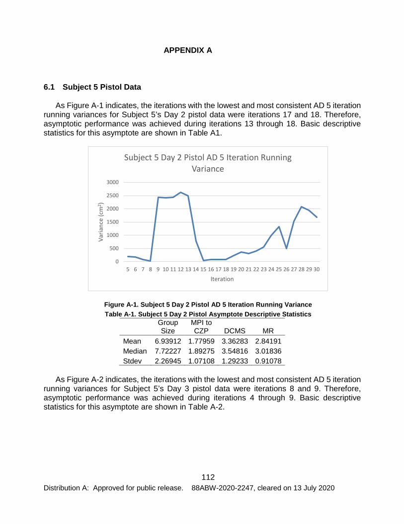
112 Distribution A: Approved for public release. 88ABW-2020-2247, cleared on 13 July 2020
APPENDIX A
6.1 Subject 5 Pistol Data
As Figure A-1 indicates, the iterations with the lowest and most consistent AD 5 iteration running variances for Subject 5’s Day 2 pistol data were iterations 17 and 18. Therefore, asymptotic performance was achieved during iterations 13 through 18. Basic descriptive statistics for this asymptote are shown in Table A1.
Figure A-1. Subject 5 Day 2 Pistol AD 5 Iteration Running Variance Table A-1. Subject 5 Day 2 Pistol Asymptote Descriptive Statistics
Group Size
MPI to CZP DCMS MR
Mean 6.93912 1.77959 3.36283 2.84191 Median 7.72227 1.89275 3.54816 3.01836 Stdev 2.26945 1.07108 1.29233 0.91078
As Figure A-2 indicates, the iterations with the lowest and most consistent AD 5 iteration running variances for Subject 5’s Day 3 pistol data were iterations 8 and 9. Therefore, asymptotic performance was achieved during iterations 4 through 9. Basic descriptive statistics for this asymptote are shown in Table A-2.
0
500
1000
1500
2000
2500
3000
5 6 7 8 9 10 11 12 13 14 15 16 17 18 19 20 21 22 23 24 25 26 27 28 29 30
Varia
nce
(cm
2 )
Iteration
Subject 5 Day 2 Pistol AD 5 Iteration Running Variance

113 Distribution A: Approved for public release. 88ABW-2020-2247, cleared on 13 July 2020
Figure A-2. Subject 5 Day 3 Pistol AD 5 Iteration Running Variance Table A-2. Subject 5 Day 3 Pistol Asymptote Descriptive Statistics
Group Size
MPI to CZP DCMS MR
Mean 7.61719 2.91069 3.75273 3.06485 Median 7.24227 2.73644 3.53861 2.79029 Stdev 4.07899 1.73644 1.72373 1.65776
As Figure A-3 indicates, the iterations with the lowest and most consistent AD 5 iteration running variances for Subject 5’s Day 4 pistol data were iterations 13 and 14. Therefore, asymptotic performance was achieved during iterations 9 through 14. Basic descriptive statistics for this asymptote are shown in Table A-3.
0200400600800
100012001400160018002000
5 6 7 8 9 10 11 12 13 14 15 16 17 18 19 20 21 22 23 24 25 26 27 28 29 30
Varia
nce
(cm
2 )
Iteration
Subject 5 Day 3 Pistol AD 5 Iteration Running Variance

114 Distribution A: Approved for public release. 88ABW-2020-2247, cleared on 13 July 2020
Figure A-3. Subject 5 Day 4 Pistol AD 5 Iteration Running Variance Table A-3. Subject 5 Day 4 Pistol Asymptote Descriptive Statistics
Group Size
MPI to CZP DCMS MR
Mean 6.56982 4.23775 4.8311 2.67117 Median 6.84682 3.91348 4.41366 2.77521 Stdev 2.12156 1.3395 1.0221 0.79142
As Figure A-4 indicates, the iterations with the lowest and most consistent AD 5 iteration running variances for Subject 5’s Day 5 pistol data were iterations 21 and 22. Therefore, asymptotic performance was achieved during iterations 17 through 22. Basic descriptive statistics for this asymptote are shown in Table A-4.
0
100
200
300
400
500
600
700
800
5 6 7 8 9 10 11 12 13 14 15 16 17 18 19 20 21 22 23 24 25 26 27 28 29 30
Varia
nce
(cm
2 )
Iteration
Subject 5 Day 4 Pistol AD 5 Iteration Running Variance

115 Distribution A: Approved for public release. 88ABW-2020-2247, cleared on 13 July 2020
Figure A-4. Subject 5 Pistol Day 5 AD 5 Iteration Running Variance Table A-4. Subject 5 Pistol Day 5 Pistol Asymptote Descriptive Statistics
Group Size
MPI to CZP DCMS MR
Mean 4.977 1.89324 2.63902 1.98048 Median 5.10147 2.14889 2.65626 1.95926 Stdev 1.00569 0.93648 0.28479 0.40062
As Table A-5 indicates, the assumption of normality could not be met for all of Subject 5’s pistol group size data. The boxplot in Figure A-5 does not provide evidence to the contrary. When Bartlett’s Test was performed on these data, the resulting K2 was 7.9205 and the p-value was 0.04769, which rejected the null hypothesis of homoscedasticity. The Brunner-Dette-Munk test yielded an F value of 1.143181 and a p-value of 0.3555183, failing to reject the null hypothesis of equality of distribution functions. As such, the analysis does not find a statistically significant difference in Subject 5’s pistol group sizes during days 2-5.
Table A-5. Subject 5 Pistol Group Size Shapiro-Wilk Test Results Day W P-Value
2 0.7901931 0.0478809 3 0.9781372 0.9419320 4 0.8240255 0.0955915 5 0.8999845 0.3738382
0100200300400500600700800900
5 6 7 8 9 10 11 12 13 14 15 16 17 18 19 20 21 22 23 24 25 26 27 28 29 30
Vara
ince
(cm
2 )
Iteration
Subject 5 Pistol Day 5 AD 5 Iteration Running Variance

116 Distribution A: Approved for public release. 88ABW-2020-2247, cleared on 13 July 2020
Figure A-5. Subject 5 Pistol Group Size Data by Day
As Table A-6 indicates, the null hypothesis of normality was rejected for day 5 of Subject 5’s pistol MPI to CZP distance data. The boxplot in Figure A-6 does not provide information to the contrary. When Bartlett’s Test was performed on these data, the resulting K2 was 2.0674 and the p-value was 0.5585, which failed to reject the null hypothesis of homoscedasticity. The Kruskal-Wallis Test yielded a Χ2 value of 9.2733 and a p-value of 0.02587, rejecting the null hypothesis of equality of dataset medians.
Table A-6. Subject 5 Pistol MPI to CZP Distance Shapiro-Wilk Test Results Day W P-Value
2 0.9793661 0.9483635 3 0.8714395 0.2320035 4 0.9209002 0.5118683 5 0.7366391 0.0146952

117 Distribution A: Approved for public release. 88ABW-2020-2247, cleared on 13 July 2020
Figure A-6. Subject 5 Pistol MPI to CZP Distance Data by Day
As Table A-7 indicates, statistically significant differences were found between days 2 and 4 and between days 4 and 5. While these differences are significant, they are not indicative of a trend, as there was no progressive change over the days of firing.
Table A-7. Subject 5 Pistol MPI to CZP Distance Dunn's Test Results Days Z P-Value 2 & 3 -1.265569 0.1543 2 & 4 -2.735263 0.0187 2 & 5 -0.244948 0.4032 3 & 4 -1.469693 0.1416 3 & 5 1.020620 0.1845 4 & 5 2.490314 0.0191
As Table A-8 indicates, the null hypothesis of normality was not rejected for Subject 5’s pistol DCMS data. The boxplot in Figure A-7, however, is not indicative of a normal distribution. When Bartlett’s Test was performed on these data, the resulting K2 was 10.754 and the p-value was 0.01314, which rejected the null hypothesis of homoscedasticity. The Brunner-Dette-Munk test yielded an F value of 4.850609 and a p-value of 0.02491593, rejecting the null hypothesis of equality of distribution functions.
Table A-8. Subject 5 Pistol DCMS Shapiro-Wilk Test Results
Day W P-Value 2 0.9573299 0.7989437 3 0.9770942 0.9362357 4 0.8254901 0.0983940 5 0.9131735 0.4576012
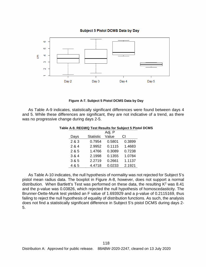
118 Distribution A: Approved for public release. 88ABW-2020-2247, cleared on 13 July 2020
Figure A-7. Subject 5 Pistol DCMS Data by Day
As Table A-9 indicates, statistically significant differences were found between days 4 and 5. While these differences are significant, they are not indicative of a trend, as there was no progressive change during days 2-5.
Table A-9. REGWQ Test Results for Subject 5 Pistol DCMS
Days Statistic Adj. P Value CI
2 & 3 0.7954 0.5801 0.3899 2 & 4 2.9952 0.1115 1.4683 2 & 5 1.4766 0.3089 0.7238 3 & 4 2.1998 0.1355 1.0784 3 & 5 2.2719 0.2661 1.1137 4 & 5 4.4718 0.0233 2.1921
As Table A-10 indicates, the null hypothesis of normality was not rejected for Subject 5’s pistol mean radius data. The boxplot in Figure A-8, however, does not support a normal distribution. When Bartlett’s Test was performed on these data, the resulting K2 was 8.41 and the p-value was 0.03826, which rejected the null hypothesis of homoscedasticity. The Brunner-Dette-Munk test yielded an F value of 1.693929 and a p-value of 0.2115169, thus failing to reject the null hypothesis of equality of distribution functions. As such, the analysis does not find a statistically significant difference in Subject 5’s pistol DCMS during days 2-5.

119 Distribution A: Approved for public release. 88ABW-2020-2247, cleared on 13 July 2020
Table A-10. Subject 5 Pistol Mean Radius Shapiro-Wilk Test Results Day W P-Value
2 0.8509817 0.1603058 3 0.9566744 0.7937793 4 0.8698722 0.2257159 5 0.8590973 0.1860907
Figure A-8. Subject 5 Pistol Mean Radius Data by Day
6.2 Subject 5 Rifle Data
As Figure A-9 indicates, the iterations with the lowest and most consistent AD 5 iteration running variances for Subject 5’s Day 2 rifle data were iterations 27 and 28. Therefore, asymptotic performance was achieved during iterations 23 through 28. Basic descriptive statistics for this asymptote are shown in Table A-11.

120 Distribution A: Approved for public release. 88ABW-2020-2247, cleared on 13 July 2020
Figure A-9. Subject 5 Day 2 Rifle AD 5 Iteration Running Variance Table A-11. Subject 5 Day 2 Rifle Asymptote Descriptive Statistics
Group Size
MPI to CZP DCMS MR
Mean 11.4613 3.64871 5.85835 4.61387 Median 12.1677 3.43198 5.55803 4.77957 Stdev 3.69824 1.33404 0.88138 1.61776
As Figure A-10 indicates, the iterations with the lowest and most consistent AD 5 iteration running variances for Subject 5’s Day 3 rifle data were iterations 19 and 20. Therefore, asymptotic performance was achieved during iterations 15 through 20. Basic descriptive statistics for this asymptote are shown in Table A-12.
0
1000
2000
3000
4000
5000
6000
7000
5 6 7 8 9 10 11 12 13 14 15 16 17 18 19 20 21 22 23 24 25 26 27 28 29 30
Varia
nce
(cm
2 )
Iteration
Subject 5 Day 2 Rifle AD 5 Iteration Running Variance

121 Distribution A: Approved for public release. 88ABW-2020-2247, cleared on 13 July 2020
Figure A-10. Subject 5 Day 3 Rifle AD 5 Iteration Running Variance Table A-12. Subject 5 Day 3 Rifle Asymptote Descriptive Statistics
Group Size
MPI to CZP DCMS MR
Mean 12.996 3.60212 5.38495 5.26779 Median 13.2033 3.41343 5.34008 5.29703 Stdev 2.0676 0.62512 0.64486 0.66754
As Figure A-11 indicates, the iterations with the lowest and most consistent AD 5 iteration running variances for Subject 5’s Day 4 rifle data were iterations 10 and 11. Therefore, asymptotic performance was achieved during iterations 6 through 11. Basic descriptive statistics for this asymptote are shown in Table A-13.
0
1000
2000
3000
4000
5000
6000
5 6 7 8 9 10 11 12 13 14 15 16 17 18 19 20 21 22 23 24 25 26 27 28 29 30
Varia
nce
(cm
2 )
Iteration
Subject 5 Day 3 Rifle AD 5 Iteration Running Variance

122 Distribution A: Approved for public release. 88ABW-2020-2247, cleared on 13 July 2020
Figure A-11. Subject 5 Day 4 Rifle AD 5 Iteration Running Variance Table A-13. Subject 5 Rifle Day 4 Asymptote Descriptive Statistics
Group Size
MPI to CZP DCMS MR
Mean 10.9855 4.27981 5.94107 4.40252 Median 10.5291 4.82597 6.57562 4.43125 Stdev 1.75601 2.55345 1.83874 0.68128
As Figure A-12 indicates, the iterations with the lowest and most consistent AD 5 iteration running variances for Subject 5’s Day 5 rifle data were iterations 16 and 17. Therefore, asymptotic performance was achieved during iterations 12 through 17. Basic descriptive statistics for this asymptote are shown in Table A-14.
0
1000
2000
3000
4000
5000
6000
5 6 7 8 9 10 11 12 13 14 15 16 17 18 19 20 21 22 23 24 25 26 27 28 29 30
Varia
nce
(cm
2 )
Iteration
Subject 5 Day 4 Rifle AD 5 Iteration Running Variance

123 Distribution A: Approved for public release. 88ABW-2020-2247, cleared on 13 July 2020
Figure A-12. Subject 5 Rifle Day 5 AD 5 Iteration Running Variance Table A-14. Subject 5 Rifle Day 5 Asymptote Descriptive Statistics
Group Size
MPI to CZP DCMS MR
Mean 10.3725 6.76124 7.68512 4.03282 Median 10.6778 6.70488 7.38607 4.16448 Stdev 1.01778 1.59484 1.62941 0.61185
As Table A-15 indicates, the null hypothesis of normality was not rejected for Subject 5’s rifle group size data. The boxplot in Figure A-13, however, does not support a normal distribution. When Bartlett’s Test was performed on these data, the resulting K2 was 7.3944 and the p-value was 0.06034, which failed to reject the null hypothesis of homoscedasticity. The Kruskal-Wallis Test yielded a Χ2 value of 6.46 and a p-value of 0.09125, thus failing to reject the null hypothesis of equality of dataset medians. As such, the analysis does not find any significant differences in rifle group size data during days 2-5.
Table A-15. Subject 5 Rifle Group Size Shapiro-Wilk Test Results Day W P-Value
2 0.8177373 0.0843533 3 0.9609670 0.8271616 4 0.9155670 0.4740200 5 0.9149908 0.4700343
0
500
1000
1500
2000
2500
3000
3500
4000
5 6 7 8 9 10 11 12 13 14 15 16 17 18 19 20 21 22 23 24 25 26 27 28 29 30
Varia
nce
(cm
2 )
Iteration
Subject 5 Rifle Day 5 AD 5 Iteration Running Variance

124 Distribution A: Approved for public release. 88ABW-2020-2247, cleared on 13 July 2020
Figure A-13. Subject 5 Rifle Group Size by Day
As Table A-16 indicates, the null hypothesis of normality was not rejected for Subject 5’s rifle MPI to CZP distance data. The boxplot in Figure A-14, however, does not support a normal distribution. When Bartlett’s Test was performed on these data, the resulting K2 was 7.7787 and the p-value was 0.0581, which failed to reject the null hypothesis of homoscedasticity. The Kruskal-Wallis Test yielded a Χ2 value of 8.98 and a p-value of 0.02956, thus rejecting the null hypothesis of equality of dataset medians.
Table A-16. Subject 5 Rifle MPI to CZP Distance Shapiro-Wilk Test Results Day W P-Value
2 0.9268055 0.5556678 3 0.8976043 0.3599627 4 0.8972969 0.3581990 5 0.9157210 0.4750886

125 Distribution A: Approved for public release. 88ABW-2020-2247, cleared on 13 July 2020
Figure A-14. Subject 5 Rifle MPI to CZP Distance by Day
As Table A-17 indicates, statistically significant differences were found only between days 2 and 5 and 3 and 5. While significant, the differences are not indicative of a progressive trend.
Table A-17. Subject 5 Rifle MPI to CZP Distance Dunn's Test Results Days Z P-Value 2 & 3 -0.040824 0.4837 2 & 4 -0.775671 0.2190 2 & 5 -2.612789 0.0045 3 & 4 -0.734846 0.2312 3 & 5 -2.571964 0.0051 4 & 5 -1.837117 0.331
As Table A-18 indicates, the null hypothesis of normality was not rejected for Subject 5’s rifle DCMS data. The boxplot in Figure A-15, however, does not support a normal distribution. When Bartlett’s Test was performed on these data, the resulting K2 was 6.011 and the p-value was 0.1111, which failed to reject the null hypothesis of homoscedasticity. The Kruskal-Wallis Test yielded a Χ2 value of 7.38 and a p-value of 0.0672, thus failing to reject the null hypothesis of equality of dataset medians. As such, the analysis does not find significant differences in rifle DCMS during days 2-5.
Table A-18. Subject 5 Rifle DCMS Shapiro-Wilk Test Results Day W P-Value

126 Distribution A: Approved for public release. 88ABW-2020-2247, cleared on 13 July 2020
2 0.8905644 0.3211556 3 0.9571090 0.7972062 4 0.8552487 0.1734517 5 0.9383441 0.6458863
Figure A-15. Subject 5 Rifle DCMS Data by Day
As Table A-19 indicates, the null hypothesis of normality was not rejected for Subject 5’s rifle mean radius data. The boxplot in Figure A-16, however, does not support a normal distribution. When Bartlett’s Test was performed on these data, the resulting K2 was 6.9062 and the p-value was 0.07495, which failed to reject the null hypothesis of homoscedasticity. The Kruskal-Wallis Test yielded a Χ2 value of 7.5 and a p-value of 0.05756, thus failing to reject the null hypothesis of equality of dataset medians. As such, the analysis is not indicative of differences in mean radius during days 2-5.
Table A-19. Subject 5 Rifle Mean Radius Shapiro-Wilk Test Results Day W P-Value
2 0.8546942 0.1716928 3 0.9435186 0.6876581 4 0.9486914 0.7296724 5 0.9507745 0.7465497

127 Distribution A: Approved for public release. 88ABW-2020-2247, cleared on 13 July 2020
Figure A-16. Subject 5 Rifle Mean Radius Data by Day
6.3 Subject 7 Pistol Data
As Figure A-17 indicates, the iterations with the lowest and most consistent AD 5 iteration running variances for Subject 7’s Day 2 pistol data were iterations 17 and 18. Therefore, asymptotic performance was achieved during iterations 13 through 18. Basic descriptive statistics for this asymptote are shown in Table A-20.
Figure A-17. Subject 7 Day 2 Pistol AD 5 Iteration Running Variance
Table A-20. Subject 7 Day 2 Pistol Asymptote Descriptive Statistics
0500
10001500200025003000350040004500
5 6 7 8 9 10 11 12 13 14 15 16 17 18 19 20 21 22 23 24 25 26 27 28 29 30
Varia
nce
(cm
2 )
Iteration
Subject 7 Day 2 Pistol AD 5 Iteration Running Variance
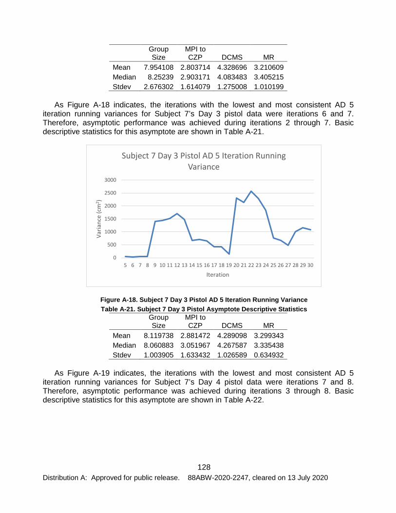
128 Distribution A: Approved for public release. 88ABW-2020-2247, cleared on 13 July 2020
Group Size
MPI to CZP DCMS MR
Mean 7.954108 2.803714 4.328696 3.210609 Median 8.25239 2.903171 4.083483 3.405215 Stdev 2.676302 1.614079 1.275008 1.010199
As Figure A-18 indicates, the iterations with the lowest and most consistent AD 5 iteration running variances for Subject 7’s Day 3 pistol data were iterations 6 and 7. Therefore, asymptotic performance was achieved during iterations 2 through 7. Basic descriptive statistics for this asymptote are shown in Table A-21.
Figure A-18. Subject 7 Day 3 Pistol AD 5 Iteration Running Variance Table A-21. Subject 7 Day 3 Pistol Asymptote Descriptive Statistics
Group Size
MPI to CZP DCMS MR
Mean 8.119738 2.881472 4.289098 3.299343 Median 8.060883 3.051967 4.267587 3.335438 Stdev 1.003905 1.633432 1.026589 0.634932
As Figure A-19 indicates, the iterations with the lowest and most consistent AD 5 iteration running variances for Subject 7’s Day 4 pistol data were iterations 7 and 8. Therefore, asymptotic performance was achieved during iterations 3 through 8. Basic descriptive statistics for this asymptote are shown in Table A-22.
0
500
1000
1500
2000
2500
3000
5 6 7 8 9 10 11 12 13 14 15 16 17 18 19 20 21 22 23 24 25 26 27 28 29 30
Varia
nce
(cm
2 )
Iteration
Subject 7 Day 3 Pistol AD 5 Iteration Running Variance

129 Distribution A: Approved for public release. 88ABW-2020-2247, cleared on 13 July 2020
Figure A-19. Subject 7 Day 4 Pistol AD 5 Iteration Running Variance Table A-22. Subject 7 Day 4 Pistol Asymptote Descriptive Statistics
Group Size
MPI to CZP DCMS MR
Mean 9.03656 5.111083 6.024767 3.513911 Median 7.701577 3.775 4.705936 2.983699 Stdev 3.187585 3.483673 2.962279 1.099067
As Figure A-20 indicates, the iterations with the lowest and most consistent AD 5 iteration running variances for Subject 7’s Day 5 pistol data were iterations 13 and 14. Therefore, asymptotic performance was achieved during iterations 9 through 14. Basic descriptive statistics for this asymptote are shown in Table A-23.
0500
10001500200025003000350040004500
5 6 7 8 9 10 11 12 13 14 15 16 17 18 19 20 21 22 23 24 25 26 27 28 29 30
Varia
nce
(cm
2 )
Iteration
Subject 7 Day 4 Pistol AD 5 Iteration Running Variance

130 Distribution A: Approved for public release. 88ABW-2020-2247, cleared on 13 July 2020
Figure A-20. Subject 7 Day 5 Pistol AD 5 Iteration Running Variance Table A-23. Subject 7 Day 5 Pistol Asymptote Descriptive Statistics
Group Size
MPI to CZP DCMS MR
Mean 12.58997 3.899054 6.059344 5.048491 Median 12.5225 4.003576 5.855018 4.887903 Stdev 1.428049 1.634954 1.063054 0.469551
As Table A-24 indicates, the null hypothesis of normality was not rejected for Subject 7’s pistol group size data. The boxplot in Figure A-21, however, does not support a normal distribution. When Bartlett’s Test was performed on these data, the resulting K2 was 6.9385 and the p-value was 0.07388, which failed to reject the null hypothesis of homoscedasticity. The Kruskal-Wallis Test yielded a Χ2 value of 10.327 and a p-value of 0.01598, thus rejecting the null hypothesis of equality of dataset medians.
Table A-24. Subject 7 Pistol Group Size Shapiro-Wilk Test Results Day W P-Value
2 0.9298284 0.5787773 3 0.9371605 0.6364137 4 0.8083995 0.0698494 5 0.9482988 0.7264860
0
1000
2000
3000
4000
5000
6000
7000
8000
5 6 7 8 9 10 11 12 13 14 15 16 17 18 19 20 21 22 23 24 25 26 27 28 29 30
Varia
nce
(cm
2 )
Iteration
Subject 7 Day 5 Pistol AD 5 Iteration Running Variance

131 Distribution A: Approved for public release. 88ABW-2020-2247, cleared on 13 July 2020
Figure A-21. Subject 7 Pistol Group Size Data by Day
As Table A-25 indicates, significant differences were found between days 2 and 5; days 3 and 5; and days 4 and 5. These differences imply an increase in group size on day 5, but not a progressive increase throughout the days of firing. As such, the analysis does not support a trend.
Table A-25. Dunn's Test Results for Subject 7 Pistol Group Size Data Days Z P-Value 2 & 3 0.24124 0.4191 2 & 4 -0.081649 0.4675 2 & 5 -2.571964 0.0051 3 & 4 -0.285773 0.3875 3 & 5 -2.776088 0.0028 4 & 5 -2.490314 0.0064
As Table A-26 indicates, the null hypothesis of normality was not rejected for Subject 7’s pistol MPI to CZP distance data. The boxplot in Figure A-22, however, does not support a normal distribution. When Bartlett’s Test was performed on these data, the resulting K2 was 4.7811 and the p-value was 0.1885, which failed to reject the null hypothesis of homoscedasticity. The Kruskal-Wallis Test yielded a Χ2 value of 2.6333 and a p-value of 0.4517, thus failing to reject the null hypothesis of equality of dataset medians. As such, the analysis did not find any significant differences in pistol MPI to CZP distance during days 2-5.
Table A-26. Subject 7 Pistol MPI to CZP Distance Shapiro-Wilk Test Results
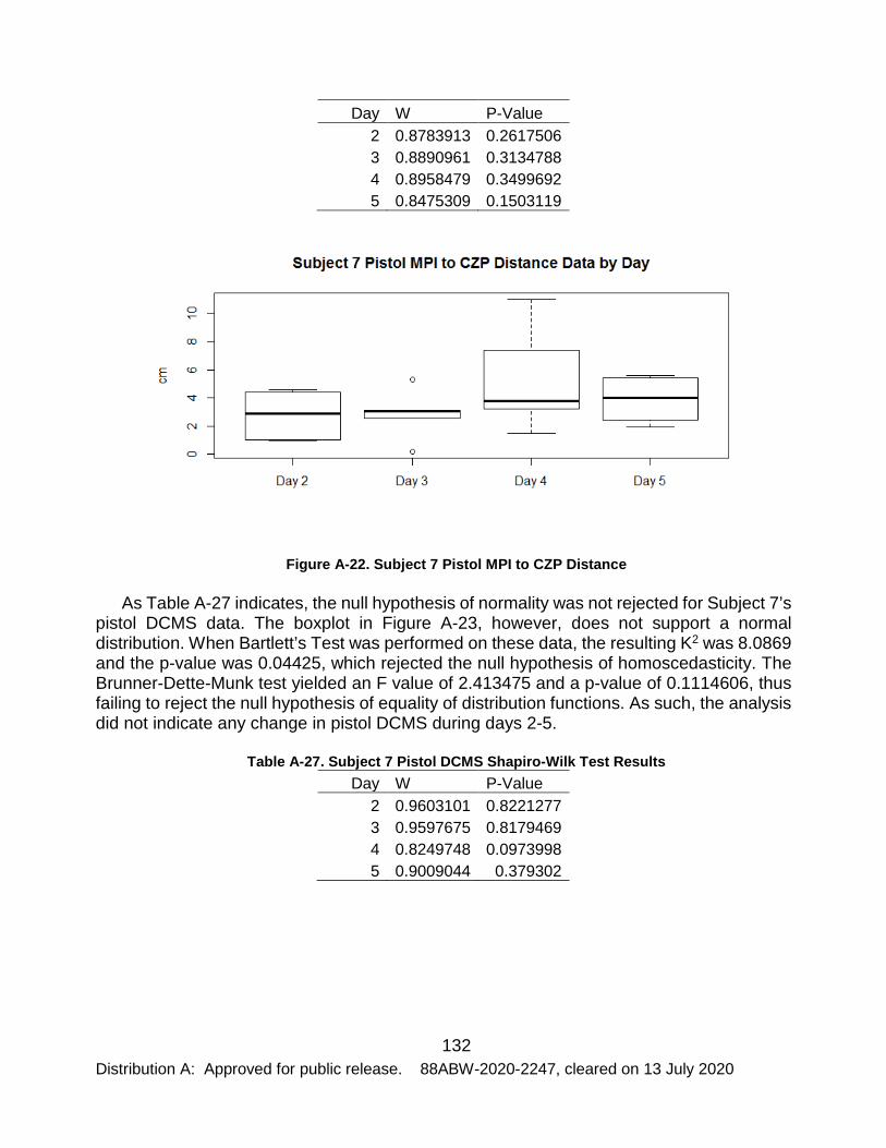
132 Distribution A: Approved for public release. 88ABW-2020-2247, cleared on 13 July 2020
Day W P-Value 2 0.8783913 0.2617506 3 0.8890961 0.3134788 4 0.8958479 0.3499692 5 0.8475309 0.1503119
Figure A-22. Subject 7 Pistol MPI to CZP Distance
As Table A-27 indicates, the null hypothesis of normality was not rejected for Subject 7’s pistol DCMS data. The boxplot in Figure A-23, however, does not support a normal distribution. When Bartlett’s Test was performed on these data, the resulting K2 was 8.0869 and the p-value was 0.04425, which rejected the null hypothesis of homoscedasticity. The Brunner-Dette-Munk test yielded an F value of 2.413475 and a p-value of 0.1114606, thus failing to reject the null hypothesis of equality of distribution functions. As such, the analysis did not indicate any change in pistol DCMS during days 2-5.
Table A-27. Subject 7 Pistol DCMS Shapiro-Wilk Test Results Day W P-Value
2 0.9603101 0.8221277 3 0.9597675 0.8179469 4 0.8249748 0.0973998 5 0.9009044 0.379302

133 Distribution A: Approved for public release. 88ABW-2020-2247, cleared on 13 July 2020
Figure A-23. Subject 7 Pistol DCMS Data
As Table A-28 indicates, the null hypothesis of normality was rejected for day 4 of Subject 7’s pistol MR data. The boxplot in Figure A-24 does not provide information to the contrary. When Bartlett’s Test was performed on these data, the resulting K2 was 3.961 and the p-value was 0.2657, which failed to reject the null hypothesis of homoscedasticity. The Kruskal-Wallis Test yielded a Χ2 value of 11.14 and a p-value of 0.01099, thus rejecting the null hypothesis of equality of dataset medians.
Table A-28. Subject 7 Pistol Mean Radius Shapiro-Wilk Test Results Day W P-Value
2 0.9409305 0.6667052 3 0.9603439 0.8223869 4 0.7889306 0.0466216 5 0.9012553 0.3814032

134 Distribution A: Approved for public release. 88ABW-2020-2247, cleared on 13 July 2020
Figure A-24. Subject 7 Pistol Mean Radius Data
As Table A-29 indicates, statistically significant differences were found between days 2 and 5; days 3 & 5; and days 4 & 5. While significant, the differences are not indicative of a progressive trend. Rather, these differences imply that the day 5 pistol mean radius data were different from all others.
Table A-29. Dunn's Test Results for Subject 7 Pistol Mean Radius Data Days Z P-Value 2 & 3 0.122474 0.5415 2 & 4 -0.040824 0.4837 2 & 5 -2.694438 0.0106 3 & 4 -0.163299 0.6527 3 & 5 -2.816913 0.0145 4 & 5 -2.653613 0.0080
6.4 Subject 7 Rifle Data
As Figure A-25 indicates, the iterations with the lowest and most consistent AD 5 iteration running variances for Subject 7’s Day 2 rifle data were iterations 28 and 29. Therefore, asymptotic performance was achieved during iterations 24 through 29. Basic descriptive statistics for this asymptote are shown in Table A-30.

135 Distribution A: Approved for public release. 88ABW-2020-2247, cleared on 13 July 2020
Figure A-25. Subject 7 Day 2 Rifle AD 5 Iteration Running Variance Table A-30. Subject 7 Day 2 Rifle Descriptive Statistics
Group Size
MPI to CZP DCMS MR
Mean 8.519608 4.202523 5.295696 3.256228 Median 9.091357 3.76449 5.024529 3.564073 Stdev 2.264408 1.639684 1.218939 0.767568
As Figure A-26 indicates, the iterations with the lowest and most consistent AD 5 iteration running variances for Subject 7’s Day 3 rifle data were iterations 26 and 27. Therefore, asymptotic performance was achieved during iterations 22 through 27. Basic descriptive statistics for this asymptote are shown in Table A-31.
0
500
1000
1500
2000
2500
5 6 7 8 9 10 11 12 13 14 15 16 17 18 19 20 21 22 23 24 25 26 27 28 29 30
Varia
nce
(cm
2 )
Iteration
Subject 7 Day 2 Rifle AD 5 Iteration Running Variance
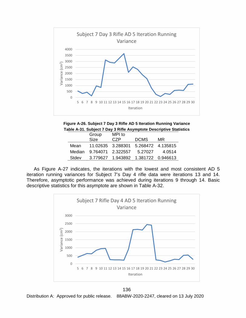
136 Distribution A: Approved for public release. 88ABW-2020-2247, cleared on 13 July 2020
Figure A-26. Subject 7 Day 3 Rifle AD 5 Iteration Running Variance Table A-31. Subject 7 Day 3 Rifle Asymptote Descriptive Statistics
Group Size
MPI to CZP DCMS MR
Mean 11.02635 3.288301 5.268472 4.135815 Median 9.764071 2.322557 5.27027 4.0514 Stdev 3.779627 1.943892 1.381722 0.946613
As Figure A-27 indicates, the iterations with the lowest and most consistent AD 5 iteration running variances for Subject 7’s Day 4 rifle data were iterations 13 and 14. Therefore, asymptotic performance was achieved during iterations 9 through 14. Basic descriptive statistics for this asymptote are shown in Table A-32.
0
500
1000
1500
2000
2500
3000
3500
4000
5 6 7 8 9 10 11 12 13 14 15 16 17 18 19 20 21 22 23 24 25 26 27 28 29 30
Varia
nce
(cm
2 )
Iteration
Subject 7 Day 3 Rifle AD 5 Iteration Running Variance
0
500
1000
1500
2000
2500
3000
5 6 7 8 9 10 11 12 13 14 15 16 17 18 19 20 21 22 23 24 25 26 27 28 29 30
Varia
nce
(cm
2 )
Iteration
Subject 7 Rifle Day 4 AD 5 Iteration Running Variance

137 Distribution A: Approved for public release. 88ABW-2020-2247, cleared on 13 July 2020
Figure A-27. Subject 7 Day 4 Rifle AD 5 Iteration Running Variance Table A-32. Subject 7 Day 4 Rifle Asymptote Descriptive Statistics
Group Size
MPI to CZP DCMS MR
Mean 7.456837 5.555495 6.462483 3.412461 Median 6.780601 5.55595 6.149925 3.064773 Stdev 2.310561 2.312154 2.413908 0.958594
As Figure A-28 indicates, the iterations with the lowest and most consistent AD 5 iteration running variances for Subject 7’s Day 5 rifle data were iterations 22 and 23. Therefore, asymptotic performance was achieved during iterations 18 through 23. Basic descriptive statistics for this asymptote are shown in Table A-33.
Figure A-28. Subject 7 Day 5 Rifle AD 5 Iteration Running Variance Table A-33. Subject 7 Day 5 Rifle Asymptote Descriptive Statistics
Group Size
MPI to CZP DCMS MR
Mean 10.30668 4.024082 5.538946 4.22214 Median 9.715975 3.676416 5.747358 4.068113 Stdev 2.501751 1.494772 1.030822 1.071511
As Table A-34 indicates, the null hypothesis of normality was not rejected for Subject 7’s rifle group size data. The boxplot in Figure A-29, however, does not support a normal distribution. When Bartlett’s Test was performed on these data, the resulting K2 was 1.7967 and the p-value was 0.6156, which failed to reject the null hypothesis of homoscedasticity. The Kruskal-Wallis Test yielded a Χ2 value of 4.86 and a p-value of 0.1823, thus failing to reject the null hypothesis of equality of dataset medians. As such, the analysis does not provide evidence indicative of a change in rifle group size during days 2-5.
0200400600800
100012001400160018002000
5 6 7 8 9 10 11 12 13 14 15 16 17 18 19 20 21 22 23 24 25 26 27 28 29 30
Varia
nce
(cm
2 )
Iteration
Subject 7 Day 5 Rifle AD 5 Iteration Running Variance

138 Distribution A: Approved for public release. 88ABW-2020-2247, cleared on 13 July 2020
Table A-34. Subject 7 Rifle Group Size Shapiro-Wilk Test Results Day W P-Value
2 0.8910881 0.3239282 3 0.8496104 0.1562676 4 0.8918936 0.3282288 5 0.9144715 0.4664601
Figure A-29. Subject 7 Rifle Group Size Data
As Table A-35 indicates, the null hypothesis of normality was not rejected for Subject 7’s rifle MPI to CZP distance data. The boxplot in Figure A-30, however, does not support a normal distribution. When Bartlett’s Test was performed on these data, the resulting K2 was 1.0429 and the p-value was 0.7909, which failed to reject the null hypothesis of homoscedasticity. The Kruskal-Wallis Test yielded a Χ2 value of 3.3 and a p-value of 0.3476, thus failing to reject the null hypothesis of equality of dataset medians. As such, the analysis does not provide evidence indicative of a change in rifle MPI to CZP distance during days 2-5.
Table A-35. Subject 7 Rifle MPI to CZP Distance Shapiro-Wilk Test Results Day W P-Value
2 0.9362513 0.6291636 3 0.7975908 0.0559066 4 0.9528649 0.7634062 5 0.9483983 0.7272937

139 Distribution A: Approved for public release. 88ABW-2020-2247, cleared on 13 July 2020
Figure A-30. Subject 7 Rifle MPI to DZP Distance Data
As Table A-36 indicates, the null hypothesis of normality was not rejected for Subject 7’s rifle DCMS data. The boxplot in Figure A-31 does not, however, support a normal distribution. When Bartlett’s test was performed on these data, the resulting K2 was 3.7346 and the p-value was 0.2916, which failed to reject the null hypothesis of homoscedasticity. The Kruskal-Wallis Test yielded a Χ2 value of 1.2797 and a p-value of 0.734, thus failing to reject the null hypothesis of equality of dataset medians. As such, the analysis does not provide evidence indicative of a change in rifle DCMS during days 2-5.
Table A-36. Subject 7 Rifle DCMS Shapiro-Wilk Test Results Day W P-Value
2 0.9401225 0.6601863 3 0.9508667 0.7472956 4 0.9871317 0.9687162 5 0.9095361 0.4333514

140 Distribution A: Approved for public release. 88ABW-2020-2247, cleared on 13 July 2020
Figure A-31. Subject 7 Rifle DCMS Data
As Table A-37 indicates, the null hypothesis of normality was not rejected for Subject 7’s rifle mean radius data. The boxplot in Figure A-32 does not, however, support a normal distribution. When Bartlett’s Test was performed on these data, the resulting K2 was 0.50649 and the p-value was 0.9175, which failed to reject the null hypothesis of homoscedasticity. The Kruskal-Wallis Test yielded a Χ2 value of 3.1986 and a p-value of 0.362, thus failing to reject the null hypothesis of equality of dataset medians. As such, the analysis does not provide evidence indicative of a change in rifle mean radius during days 2-5.
Table A-37. Subject 7 Rifle Mean Radius Shapiro-Wilk Test Results Day W P-Value
2 0.8456079 0.1449089 3 0.9207980 0.5111273 4 0.8944972 0.3802228 5 0.9393051 0.6536049

141 Distribution A: Approved for public release. 88ABW-2020-2247, cleared on 13 July 2020
Figure A-32. Subject 7 Rifle Mean Radius Data
6.5 Subject 8 Pistol Data
As Figure A-33 indicates, the iterations with the lowest and most consistent AD 5 iteration running variances for Subject 8’s Day 2 pistol data were iterations 28 and 29. Therefore, asymptotic performance was achieved during iterations 24 through 29. Basic descriptive statistics for this asymptote are shown in Table A-38.
Figure A-33. Subject 8 Pistol Day 2 AD 5 Iteration Running Variance
Table A-38. Subject 8 Pistol Day 2 Asymptote Descriptive Statistics
02000400060008000
100001200014000160001800020000
5 6 7 8 9 10 11 12 13 14 15 16 17 18 19 20 21 22 23 24 25 26 27 28 29 30
Varia
nce
(cm
2 )
Iteration
Subject 8 Pistol Day 2 AD 5 Iteration Running Variance

142 Distribution A: Approved for public release. 88ABW-2020-2247, cleared on 13 July 2020
Group Size
MPI to CZP DCMS MR
Mean 8.43723 3.6904 5.09241 3.47533 Median 8.97857 3.30571 5.02982 3.62457 Stdev 3.6019 2.3936 1.53353 1.64906
As Figure A-34 indicates, the iterations with the lowest and most consistent AD 5 iteration running variances for Subject 8’s Day 3 pistol data were iterations 13 and 14. Therefore, asymptotic performance was achieved during iterations 9 through 14. Basic descriptive statistics for this asymptote are shown in Table A-39.
Figure A-34. Subject 8 Pistol Day 3 AD 5 Iteration Running Variance Table A-39. Subject 8 Pistol Day 3 Asymptote Descriptive Statistics
Group Size
MPI to CZP DCMS MR
Mean 9.61127 2.76553 4.85536 3.7802 Median 9.50962 2.48838 5.49886 3.90329 Stdev 3.68784 2.14848 1.74345 1.34752
As Figure A-35 indicates, the iterations with the lowest and most consistent AD 5 iteration running variances for Subject 8’s Day 4 pistol data were iterations 18 and 19. Therefore, asymptotic performance was achieved during iterations 14 through 19. Basic descriptive statistics for this asymptote are shown in Table A-40.
0500
100015002000250030003500400045005000
5 6 7 8 9 10 11 12 13 14 15 16 17 18 19 20 21 22 23 24 25 26 27 28 29 30
Varia
nce
(cm
2 )
Iteration
Subject 8 Pistol Day 3 AD 5 Iteration Running Variance
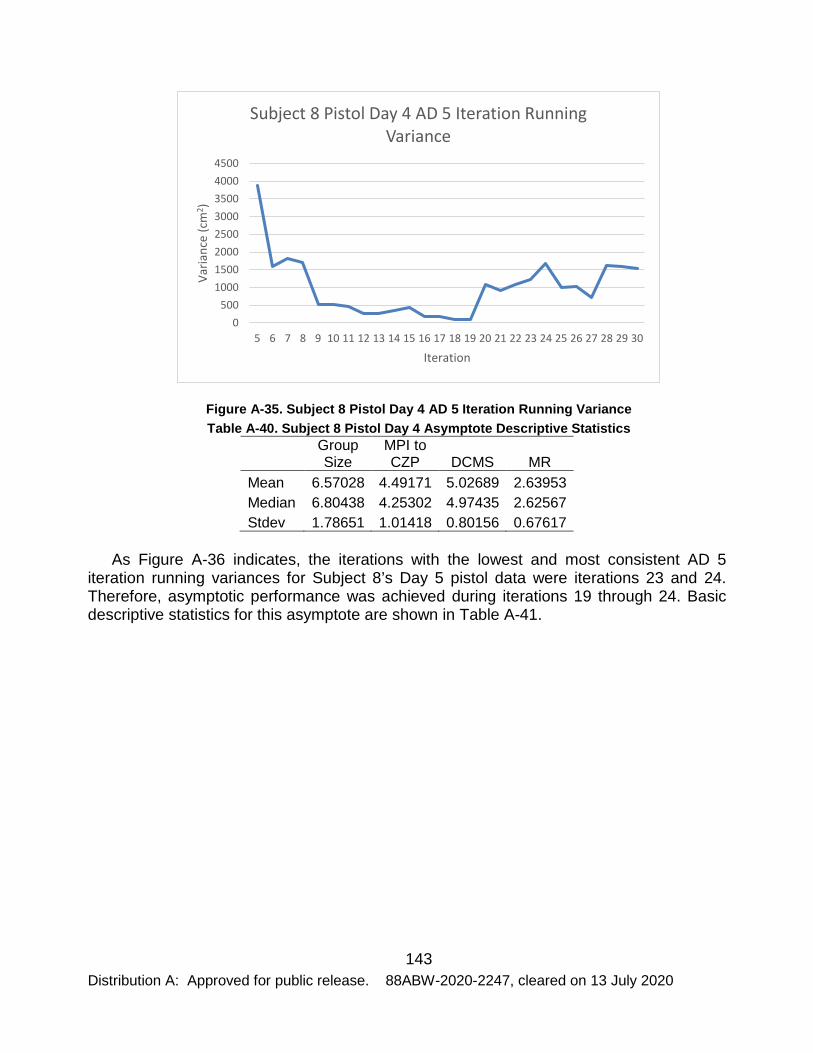
143 Distribution A: Approved for public release. 88ABW-2020-2247, cleared on 13 July 2020
Figure A-35. Subject 8 Pistol Day 4 AD 5 Iteration Running Variance Table A-40. Subject 8 Pistol Day 4 Asymptote Descriptive Statistics
Group Size
MPI to CZP DCMS MR
Mean 6.57028 4.49171 5.02689 2.63953 Median 6.80438 4.25302 4.97435 2.62567 Stdev 1.78651 1.01418 0.80156 0.67617
As Figure A-36 indicates, the iterations with the lowest and most consistent AD 5 iteration running variances for Subject 8’s Day 5 pistol data were iterations 23 and 24. Therefore, asymptotic performance was achieved during iterations 19 through 24. Basic descriptive statistics for this asymptote are shown in Table A-41.
0500
10001500200025003000350040004500
5 6 7 8 9 10 11 12 13 14 15 16 17 18 19 20 21 22 23 24 25 26 27 28 29 30
Varia
nce
(cm
2 )
Iteration
Subject 8 Pistol Day 4 AD 5 Iteration Running Variance

144 Distribution A: Approved for public release. 88ABW-2020-2247, cleared on 13 July 2020
Figure A-36. Subject 8 Pistol Day 5 AD 5 Iteration Running Variance Table A-41. Subject 8 Pistol Day 5 Asymptote Descriptive Statistics
Group Size
MPI to CZP DCMS MR
Mean 6.01746 3.97873 4.68379 2.52623 Median 6.27041 3.56488 4.61761 2.59699 Stdev 1.99604 1.97952 1.65352 0.84855
As Table A-42 indicates, the null hypothesis of normality was not rejected for Subject 8’s pistol group size data. The boxplot in Figure A-37 does not, however, support a normal distribution. When Bartlett’s Test was performed on these data, the resulting K2 was 3.7608 and the p-value was 0.2885, which failed to reject the null hypothesis of homoscedasticity. The Kruskal-Wallis Test yielded a Χ2 value of 4.2067 and a p-value of 0.243, thus failing to reject the null hypothesis of equality of dataset medians. As such, the analysis does not provide evidence indicative of a change in pistol group size during days 2-5.
Table A-42. Subject 8 Pistol Group Size Shapiro-Wilk Test Results Day W P-Value
2 0.9243959 0.5375699 3 0.8738546 0.2420068 4 0.9584184 0.8074723 5 0.9261312 0.5505734
0
200
400
600
800
1000
1200
1400
5 6 7 8 9 10 11 12 13 14 15 16 17 18 19 20 21 22 23 24 25 26 27 28 29 30
Varia
nce
(cm
2 )
Iteration
Subject 8 Pistol Day 5 AD 5 Iteration Running Variance

145 Distribution A: Approved for public release. 88ABW-2020-2247, cleared on 13 July 2020
Figure A-37. Subject 8 Pistol Group Size Data
As Table A-43 indicates, the null hypothesis of normality was not rejected for Subject 8’s pistol MPI to CZP distance data. The boxplot in Figure A-38 does not, however, support a normal distribution. When Bartlett’s Test was performed on these data, the resulting K2 was 3.2088 and the p-value was 0.3605, which failed to reject the null hypothesis of homoscedasticity. The Kruskal-Wallis Test yielded a Χ2 value of 3.7133 and a p-value of 0.29, thus failing to reject the null hypothesis of equality of dataset medians. As such, the analysis does not provide evidence of a change in pistol MPI to CZP distance during days 2-5.
Table A-43. Subject 8 Pistol MPI to CZP Distance Shapiro-Wilk Test Results Day W P-Value
2 0.9491215 0.7331616 3 0.8655021 0.2088570 4 0.9410110 0.6673552 5 0.8938872 0.3396086

146 Distribution A: Approved for public release. 88ABW-2020-2247, cleared on 13 July 2020
Figure A-38. Subject 8 Pistol MPI to CZP Distance Data
As Table A-44 indicates, the null hypothesis of normality was not rejected for Subject 8’s pistol DCMS data. The boxplot in Figure A-39 does not, however, support a normal distribution. When Bartlett’s Test was performed on these data, the resulting K2 was 2.8105 and the p-value was 0.4218, which failed to reject the null hypothesis of homoscedasticity. The Kruskal-Wallis Test yielded a Χ2 value of 0.20667 and a p-value of 0.9765, thus failing to reject the null hypothesis of equality of dataset medians. As such, the analysis does not provide evidence of a change in pistol DCMS during days 2-5.
Table A-44. Subject 8 Pistol DCMS Shapiro-Wilk Test Results Day W P-Value
2 0.9458603 0.7066748 3 0.9030025 0.3919813 4 0.8397393 0.1297179 5 0.9876601 0.9827030

147 Distribution A: Approved for public release. 88ABW-2020-2247, cleared on 13 July 2020
Figure A-39. Subject 8 Pistol DCMS Data
As Table A-45 indicates, the null hypothesis of normality was not rejected for Subject 8’s pistol mean radius data. The boxplot in Figure A-40 does not, however, support a normal distribution. When Bartlett’s Test was performed on these data, the resulting K2 was 4.3364 and the p-value was 0.2274, which failed to reject the null hypothesis of homoscedasticity. The Kruskal-Wallis Test yielded a Χ2 value of 3.26 and a p-value of 0.3532, thus failing to reject the null hypothesis of equality of dataset medians. As such, the analysis does not provide evidence of a change in mean radius during days 2-5.
Table A-45. Subject 8 Pistol Mean Radius Shapiro-Wilk Test Results Day W P-Value
2 0.8783494 0.2615627 3 0.8899330 0.3178369 4 0.9549667 0.7802312 5 0.9345606 0.6157518

148 Distribution A: Approved for public release. 88ABW-2020-2247, cleared on 13 July 2020
Figure A-40. Subject 8 Pistol Mean Radius Data
6.6 Subject 8 Rifle Data
As Figure A-41 indicates, the iterations with the lowest and most consistent AD 5 iteration running variances for Subject 8’s Day 2 rifle data were iterations 6 and 7. Therefore, asymptotic performance was achieved during iterations 2 through 7. Basic descriptive statistics for this asymptote are shown in Table A-46.
Figure A-41. Subject 8 Day 2 Rifle AD 5 Iteration Running Variances
Table A-46. Subject 8 Day 2 Rifle Asymptote Descriptive Statistics
0100020003000400050006000700080009000
10000
5 6 7 8 9 10 11 12 13 14 15 16 17 18 19 20 21 22 23 24 25 26 27 28 29 30
Varia
nce
(cm
2 )
Iteration
Subject 8 Day 2 Rifle AD 5 Iteration Running Variance

149 Distribution A: Approved for public release. 88ABW-2020-2247, cleared on 13 July 2020
Group Size
MPI to CZP DCMS MR
Mean 12.53417 5.93198 7.503408 5.067068 Median 11.45876 6.212117 7.127643 4.623409 Stdev 3.018505 3.419964 3.519961 1.256017
As Figure A-42 indicates, the iterations with the lowest and most consistent AD 5 iteration running variances for Subject 8’s Day 3 rifle data were iterations 6 and 7. Therefore, asymptotic performance was achieved during iterations 2 through 7. Basic descriptive statistics for this asymptote are shown in Table A-47.
Figure A-42. Subject 8 Day 3 Rifle AD 5 Iteration Running Variance Table A-47. Subject 8 Day 3 Rifle Asymptote Descriptive Statistics
Group Size
MPI to CZP DCMS MR
Mean 10.22995 9.484427 10.14195 4.12187 Median 9.692537 8.974528 9.58891 3.938469 Stdev 2.65252 4.777667 4.35794 1.232474
As Figure A-43 indicates, the iterations with the lowest and most consistent AD 5 iteration running variances for Subject 8’s Day 4 rifle data were iterations 13 and 14. Therefore, asymptotic performance was achieved during iterations 9 through 14. Basic descriptive statistics for this asymptote are shown in Table A-48.
0100020003000400050006000700080009000
10000
5 6 7 8 9 10 11 12 13 14 15 16 17 18 19 20 21 22 23 24 25 26 27 28 29 30
Varia
nce
(cm
2 )
Iteration
Subject 8 Day 3 Rifle AD 5 Iteration Running Variance

150 Distribution A: Approved for public release. 88ABW-2020-2247, cleared on 13 July 2020
Figure A-43. Subject 8 Day 4 Rifle AD 5 Iteration Running Variance Table A-48. Subject 8 Day 4 Rifle Asymptote Descriptive Statistics
Group Size
MPI to CZP DCMS MR
Mean 10.86444 7.83432 8.856091 4.422953 Median 9.856523 8.886165 9.195886 4.150009 Stdev 3.483495 3.216469 2.017545 1.134533
As Figure A-44 indicates, the iterations with the lowest and most consistent AD 5 iteration running variances for Subject 8’s Day 2 rifle data were iterations 28 and 29. Therefore, asymptotic performance was achieved during iterations 24 through 29. Basic descriptive statistics for this asymptote are shown in Table A-49.
0
2000
4000
6000
8000
10000
12000
5 6 7 8 9 10 11 12 13 14 15 16 17 18 19 20 21 22 23 24 25 26 27 28 29 30
Varia
nce
(cm
2 )
Iteration
Subject 8 Day 4 Rifle AD 5 Iteration Running Variance

151 Distribution A: Approved for public release. 88ABW-2020-2247, cleared on 13 July 2020
Figure A-44. Subject 8 Day 5 Rifle AD 5 Iteration Running Variance Table A-49. Subject 8 Day 5 Rifle Asymptote Descriptive Statistics
Group Size
MPI to CZP DCMS MR
Mean 10.34722 6.805636 7.77708 4.065884 Median 11.05756 6.441898 7.525453 4.124809 Stdev 2.398319 1.271123 0.927718 0.8052
As Table A-50 indicates, the null hypothesis of normality was rejected for day 4 of Subject 8’s rifle group size data. The boxplot in Figure A-45 does not provide information to the contrary. When Bartlett’s Test was performed on these data, the resulting K2 was 0.72969 and the p-value was 0.8662, which failed to reject the null hypothesis of homoscedasticity. The Kruskal-Wallis Test yielded a Χ2 value of 2.82 and a p-value of 0.4202, thus failing to reject the null hypothesis of equality of dataset medians. As such, the analysis does not provide evidence of a change in group size during days 2-5.
Table A-50. Subject 8 Rifle Group Size Shapiro-Wilk Test Results Day W P-Value
2 0.9108802 0.4422123 3 0.8949721 0.3450634 4 0.7780648 0.0369750 5 0.9258933 0.5487817
0
1000
2000
3000
4000
5000
6000
7000
5 6 7 8 9 10 11 12 13 14 15 16 17 18 19 20 21 22 23 24 25 26 27 28 29 30
Varia
nce
(cm
2 )
Iteration
Subject 8 Day 5 Rifle AD 5 Iteration Running Variance
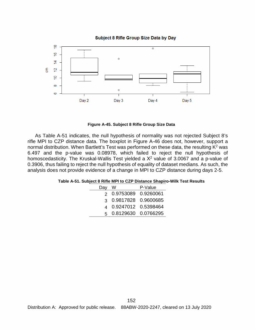
152 Distribution A: Approved for public release. 88ABW-2020-2247, cleared on 13 July 2020
Figure A-45. Subject 8 Rifle Group Size Data
As Table A-51 indicates, the null hypothesis of normality was not rejected Subject 8’s rifle MPI to CZP distance data. The boxplot in Figure A-46 does not, however, support a normal distribution. When Bartlett’s Test was performed on these data, the resulting K2 was 6.497 and the p-value was 0.08978, which failed to reject the null hypothesis of homoscedasticity. The Kruskal-Wallis Test yielded a Χ2 value of 3.0067 and a p-value of 0.3906, thus failing to reject the null hypothesis of equality of dataset medians. As such, the analysis does not provide evidence of a change in MPI to CZP distance during days 2-5.
Table A-51. Subject 8 Rifle MPI to CZP Distance Shapiro-Wilk Test Results Day W P-Value
2 0.9753089 0.9260061 3 0.9817828 0.9600685 4 0.9247012 0.5398464 5 0.8129630 0.0766295
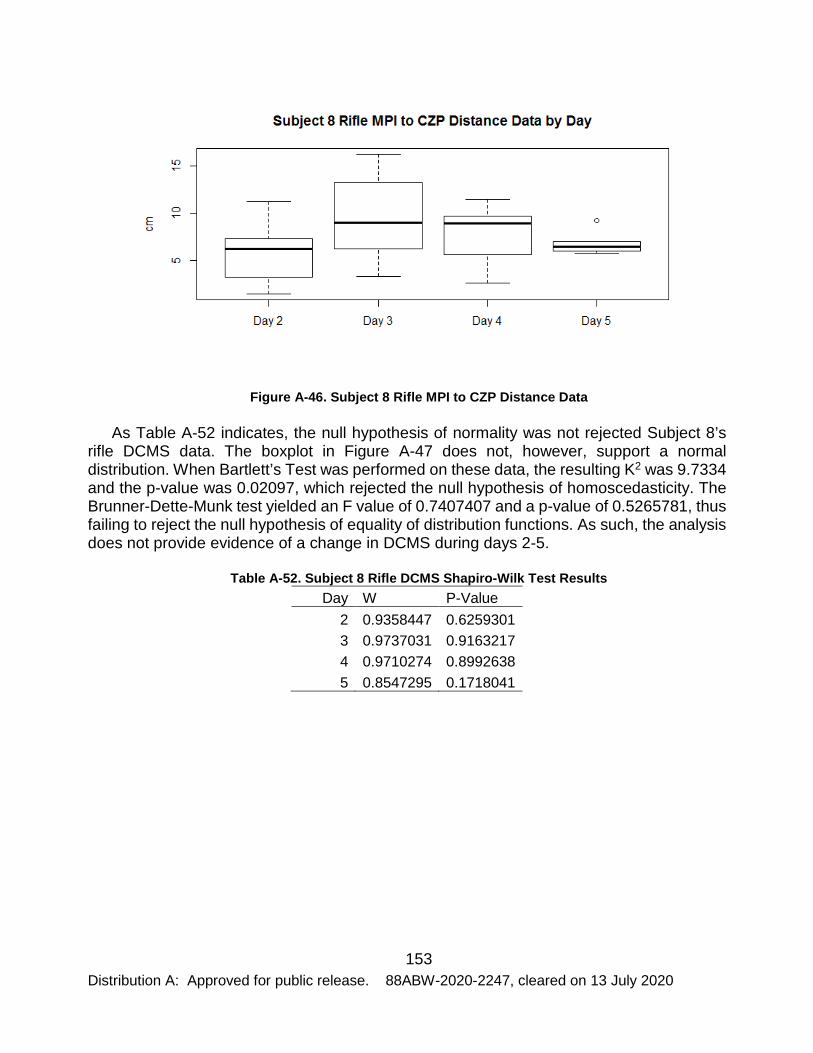
153 Distribution A: Approved for public release. 88ABW-2020-2247, cleared on 13 July 2020
Figure A-46. Subject 8 Rifle MPI to CZP Distance Data
As Table A-52 indicates, the null hypothesis of normality was not rejected Subject 8’s rifle DCMS data. The boxplot in Figure A-47 does not, however, support a normal distribution. When Bartlett’s Test was performed on these data, the resulting K2 was 9.7334 and the p-value was 0.02097, which rejected the null hypothesis of homoscedasticity. The Brunner-Dette-Munk test yielded an F value of 0.7407407 and a p-value of 0.5265781, thus failing to reject the null hypothesis of equality of distribution functions. As such, the analysis does not provide evidence of a change in DCMS during days 2-5.
Table A-52. Subject 8 Rifle DCMS Shapiro-Wilk Test Results Day W P-Value
2 0.9358447 0.6259301 3 0.9737031 0.9163217 4 0.9710274 0.8992638 5 0.8547295 0.1718041

154 Distribution A: Approved for public release. 88ABW-2020-2247, cleared on 13 July 2020
Figure A-47. Subject 8 Rifle DCMS Data
As Table A-53 indicates, the null hypothesis of normality was not rejected for Subject 8’s rifle mean radius data. The boxplot in Figure A-48 does not, however, support a normal distribution. When Bartlett’s Test was performed on these data, the resulting K2 was 1.039 and the p-value was 0.7918, which failed to reject the null hypothesis of homoscedasticity. The Kruskal-Wallis Test yielded a Χ2 value of 2.94 and a p-value of 0.401, thus failing to reject the null hypothesis of equality of dataset medians. As such, the analysis does not provide evidence of a change in mean radius during days 2-5.
Table A-53. Subject 8 Rifle Mean Radius Shapiro-Wilk Test Results Day W P-Value
2 0.8953439 0.3471397 3 0.9306888 0.5854312 4 0.7995011 0.581695 5 0.9857828 0.9764321
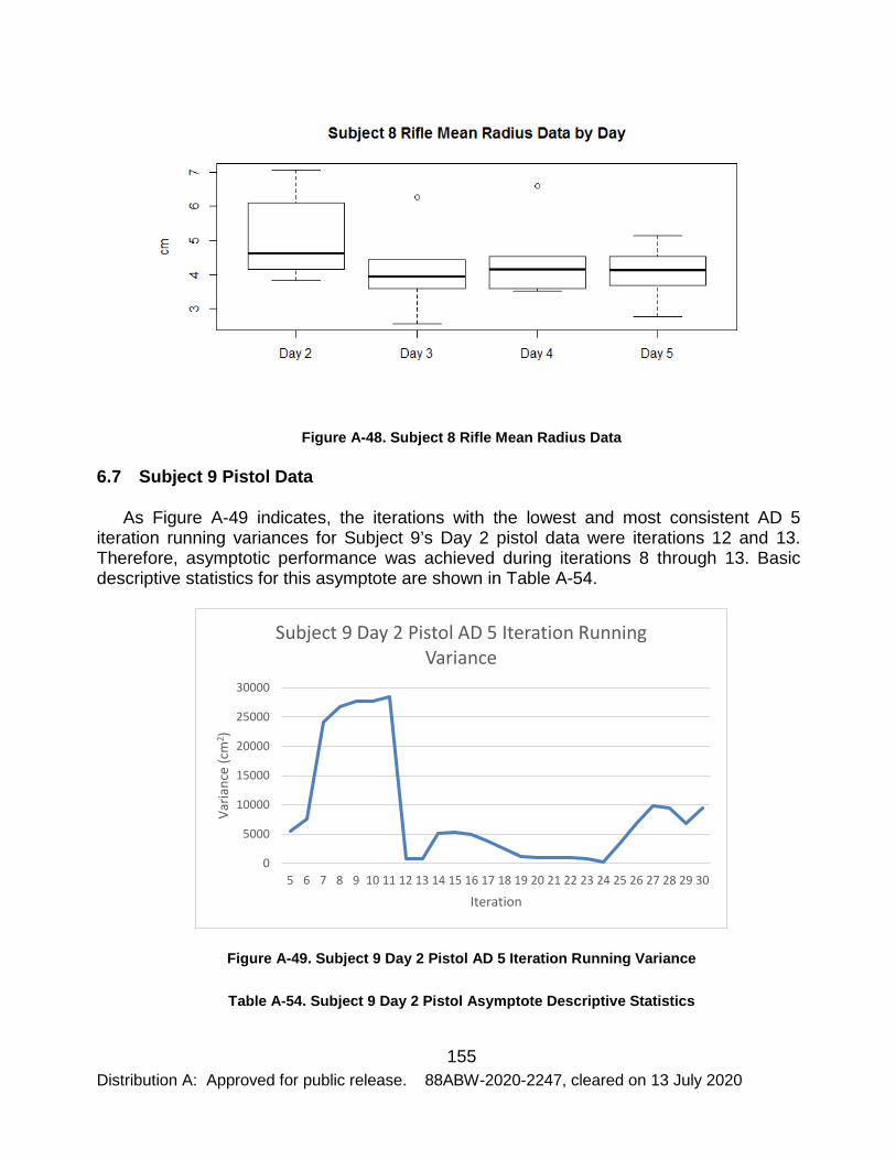
155 Distribution A: Approved for public release. 88ABW-2020-2247, cleared on 13 July 2020
Figure A-48. Subject 8 Rifle Mean Radius Data
6.7 Subject 9 Pistol Data
As Figure A-49 indicates, the iterations with the lowest and most consistent AD 5 iteration running variances for Subject 9’s Day 2 pistol data were iterations 12 and 13. Therefore, asymptotic performance was achieved during iterations 8 through 13. Basic descriptive statistics for this asymptote are shown in Table A-54.
Figure A-49. Subject 9 Day 2 Pistol AD 5 Iteration Running Variance
Table A-54. Subject 9 Day 2 Pistol Asymptote Descriptive Statistics
0
5000
10000
15000
20000
25000
30000
5 6 7 8 9 10 11 12 13 14 15 16 17 18 19 20 21 22 23 24 25 26 27 28 29 30
Varia
nce
(cm
2 )
Iteration
Subject 9 Day 2 Pistol AD 5 Iteration Running Variance

156 Distribution A: Approved for public release. 88ABW-2020-2247, cleared on 13 July 2020
Group Size
MPI to CZP DCMS MR
Mean 16.3769 8.67452 10.8418 6.35279 Median 15.0585 9.04423 9.98241 6.26341 Stdev 8.74869 2.65293 2.14104 3.15648
As Figure A-50 indicates, the iterations with the lowest and most consistent AD 5 iteration running variances for Subject 9’s Day 3 pistol data were iterations 16 and 17. Therefore, asymptotic performance was achieved during iterations 12 through 17. Basic descriptive statistics for this asymptote are shown in Table A-55.
Figure A-50. Subject 9 Day 3 Pistol AD 5 Iteration Running Variance Table A-55. Subject 9 Day 3 Pistol Asymptote Descriptive Statistics
Group Size
MPI to CZP DCMS MR
Mean 9.43583 5.90781 6.51505 3.88172 Median 7.63154 5.42995 5.8039 3.17751 Stdev 5.53337 3.02575 3.10794 2.38673
As Figure A-51 indicates, the iterations with the lowest and most consistent AD 5 iteration running variances for Subject 9’s Day 4 pistol data were iterations 29 and 30. Therefore, asymptotic performance was achieved during iterations 25 through 30. Basic descriptive statistics for this asymptote are shown in Table A-56.
0
5000
10000
15000
20000
25000
5 6 7 8 9 10 11 12 13 14 15 16 17 18 19 20 21 22 23 24 25 26 27 28 29 30
Varia
nce
(cm
2 )
Iteration
Subject 9 Day 3 Pistol AD 5 Iteration Running Variance

157 Distribution A: Approved for public release. 88ABW-2020-2247, cleared on 13 July 2020
Figure A-51. Subject 9 Day 4 Pistol AD 5 Iteration Running Variance Table A-56. Subject 9 Day 4 Pistol Asymptote Descriptive Statistics
Group Size
MPI to CZP DCMS MR
Mean 11.2538 5.46427 6.87856 4.58969 Median 11.6393 4.40753 6.29918 4.79171 Stdev 2.14391 3.17753 2.63769 1.00758
As Figure A-52 indicates, the iterations with the lowest and most consistent AD 5 iteration running variances for Subject 9’s Day 4 pistol data were iterations 13 and 14. Therefore, asymptotic performance was achieved during iterations 9 through 14. Basic descriptive statistics for this asymptote are shown in Table A-57.
0
2000
4000
6000
8000
10000
12000
14000
16000
5 6 7 8 9 10 11 12 13 14 15 16 17 18 19 20 21 22 23 24 25 26 27 28 29 30
Varia
nce
(cm
2 )
Iteration
Subject 9 Day 4 Pistol AD 5 Iteration Running Variance
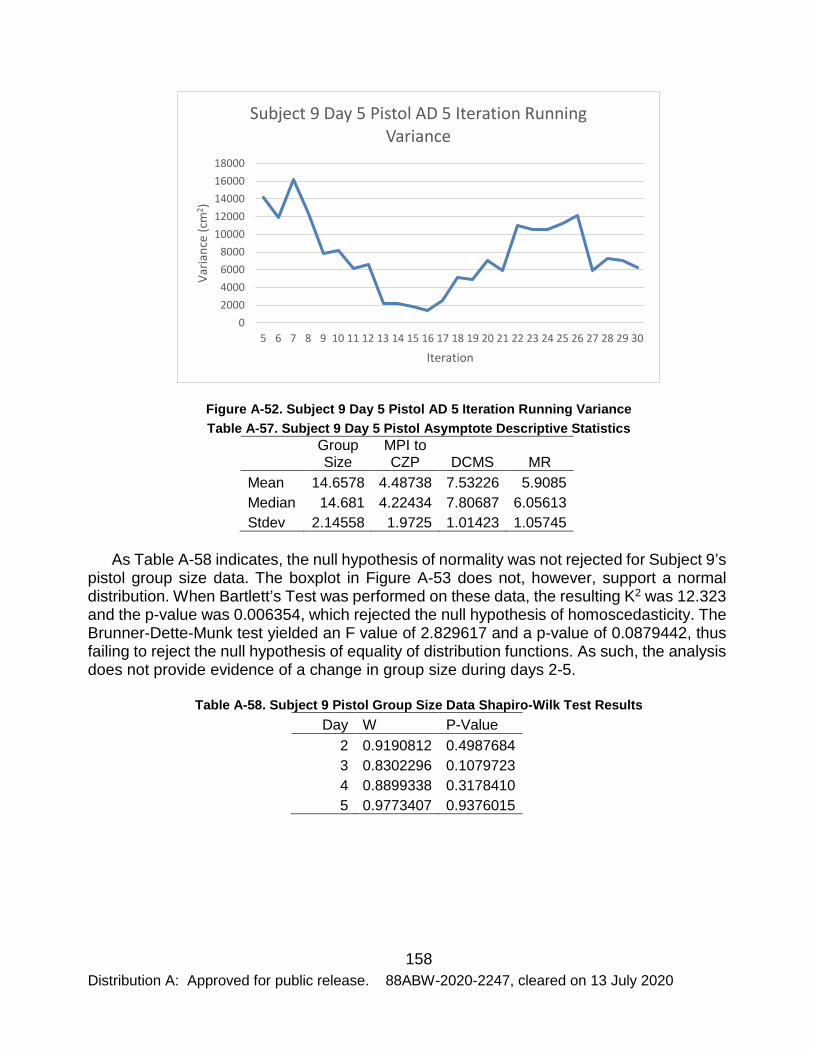
158 Distribution A: Approved for public release. 88ABW-2020-2247, cleared on 13 July 2020
Figure A-52. Subject 9 Day 5 Pistol AD 5 Iteration Running Variance Table A-57. Subject 9 Day 5 Pistol Asymptote Descriptive Statistics
Group Size
MPI to CZP DCMS MR
Mean 14.6578 4.48738 7.53226 5.9085 Median 14.681 4.22434 7.80687 6.05613 Stdev 2.14558 1.9725 1.01423 1.05745
As Table A-58 indicates, the null hypothesis of normality was not rejected for Subject 9’s pistol group size data. The boxplot in Figure A-53 does not, however, support a normal distribution. When Bartlett’s Test was performed on these data, the resulting K2 was 12.323 and the p-value was 0.006354, which rejected the null hypothesis of homoscedasticity. The Brunner-Dette-Munk test yielded an F value of 2.829617 and a p-value of 0.0879442, thus failing to reject the null hypothesis of equality of distribution functions. As such, the analysis does not provide evidence of a change in group size during days 2-5.
Table A-58. Subject 9 Pistol Group Size Data Shapiro-Wilk Test Results Day W P-Value
2 0.9190812 0.4987684 3 0.8302296 0.1079723 4 0.8899338 0.3178410 5 0.9773407 0.9376015
02000400060008000
1000012000140001600018000
5 6 7 8 9 10 11 12 13 14 15 16 17 18 19 20 21 22 23 24 25 26 27 28 29 30
Varia
nce
(cm
2 )
Iteration
Subject 9 Day 5 Pistol AD 5 Iteration Running Variance

159 Distribution A: Approved for public release. 88ABW-2020-2247, cleared on 13 July 2020
Figure A-53. Subject 9 Pistol Group Size Data
As Table A-59 indicates, the null hypothesis of normality was rejected for day 4 of Subject 9’s pistol MPI to CZP distance. The boxplot in Figure A-54 does not provide information to the contrary. When Bartlett’s Test was performed on these data, the resulting K2 was 1.1408 and the p-value was 0.7672, which failed to reject the null hypothesis of homoscedasticity. The Kruskal-Wallis Test yielded a Χ2 value of 6.58 and a p-value of 0.08656, thus failing to reject the null hypothesis of equality of dataset medians. As such, the analysis does not provide evidence of a change in MPI to CZP distance during days 2-5.
Table A-59. Subject 9 Pistol MPI to CZP Distance Shapiro-Wilk Test Results Day W P-Value
2 0.9618024 0.8335189 3 0.9564445 0.7919626 4 0.7915947 0.0493153 5 0.9556574 0.7857258

160 Distribution A: Approved for public release. 88ABW-2020-2247, cleared on 13 July 2020
Figure A-54. Subject 9 Pistol MPI to CZP Distance Data
As Table A-60 indicates, the null hypothesis of normality was not rejected for Subject 9’s pistol DCMS. The boxplot in Figure A-55 does not, however, support a normal distribution. When Bartlett’s Test was performed on these data, the resulting K2 was 5.0587 and the p-value was 0.1656, which failed to reject the null hypothesis of homoscedasticity. The Kruskal-Wallis Test yielded a Χ2 value of 10.3 and a p-value of 0.01618, thus rejecting the null hypothesis of equality of dataset medians.
Table A-60. Subject 9 Pistol DCMS Shapiro-Wilk Test Results Day W P-Value
2 0.8526823 0.1654385 3 0.9357896 0.6254922 4 0.8447170 0.1425677 5 0.9452874 0.7020197

161 Distribution A: Approved for public release. 88ABW-2020-2247, cleared on 13 July 2020
Figure A-55. Subject 9 Pistol DCMS Data
As Table A-61 indicates, significant differences were found between days 2 and 3 and days 2 and 4. These differences imply a reduction in DCMS over the course of the days of firing. The difference between days 2 and 5 is not significant because the P-value must be less than half of the alpha value of 0.05 in order to reject the null hypothesis for Dunn’s test.
Table A-61. Subject 9 Pistol DCMS Dunn's Test Results Days Z P-Value 2 & 3 2.816913 0.0024 2 & 4 2.735263 0.0031 2 & 5 1.95591 0.0250 3 & 4 -0.081649 0.4675 3 & 5 0.857321 0.1956 4 & 5 -0.775671 0.2190
As Table A-62 indicates, the null hypothesis of normality was rejected for day 4 of Subject 9’s pistol mean radius data. The boxplot in Figure A-56 does not provide information to the contrary. When Bartlett’s Test was performed on these data, the resulting K2 was 8.3285 and the p-value was 0.03969, which rejected the null hypothesis of homoscedasticity. The Brunner-Dette-Munk test yielded an F value of 1.912222 and a p-value of 0.1768024, thus failing to reject the null hypothesis of equality of distribution functions. As such, the analysis provides no evidence of a change in mean radius during days 2-5.
Table A-62. Subject 9 Pistol Mean Radius Shapiro-Wilk Test Results Day W P-Value

162 Distribution A: Approved for public release. 88ABW-2020-2247, cleared on 13 July 2020
2 0.9618024 0.8335189 3 0.9564445 0.7919626 4 0.7915947 0.0493153 5 0.9556574 0.7857258
Figure A-56. Subject 9 Pistol Mean Radius Data
6.8 Subject 9 Rifle Data
As Figure A-57 indicates, the iterations with the lowest and most consistent AD 5 iteration running variances for Subject 9’s Day 2 rifle data were iterations 25 and 26. Therefore, asymptotic performance was achieved during iterations 21 through 26. Basic descriptive statistics for this asymptote are shown in Table A-63.
0
2000
4000
6000
8000
10000
12000
5 6 7 8 9 10 11 12 13 14 15 16 17 18 19 20 21 22 23 24 25 26 27 28 29 30
Varia
nce
(cm
2 )
Iteration
Subject 9 Day 2 Rifle AD 5 Iteration Running Variance

163 Distribution A: Approved for public release. 88ABW-2020-2247, cleared on 13 July 2020
Figure A-57. Subject 9 Day 2 Rifle AD 5 Iteration Running Variance Table A-63. Subject 9 Day 2 Rifle Asymptote Descriptive Statistics
Group Size
MPI to CZP DCMS MR
Mean 13.1061 6.36123 7.96399 5.36892 Median 12.8406 6.42102 8.02803 5.48377 Stdev 3.2368 2.21585 1.6535 1.21717
As Figure A-58 indicates, the iterations with the lowest and most consistent AD 5 iteration running variances for Subject 9’s Day 3 rifle data were iterations 12 and 13. Therefore, asymptotic performance was achieved during iterations 8 through 13. Basic descriptive statistics for this asymptote are shown in Table A-64.
Figure A-58. Subject 9 Day 3 Rifle AD 5 Iteration Running Variance Table A-64. Subject 9 Day 3 Rifle Asymptote Descriptive Statistics
Group Size
MPI to CZP DCMS MR
Mean 9.95233 7.19032 8.05226 4.04167 Median 9.55282 8.34874 8.74475 3.90543 Stdev 3.0756 2.87562 2.41274 1.31104
As Figure A-59 indicates, the iterations with the lowest and most consistent AD 5 iteration running variances for Subject 9’s Day 4 rifle data were iterations 14 and 15. Therefore, asymptotic performance was achieved during iterations 10 through 15. Basic descriptive statistics for this asymptote are shown in Table A-65.
0
1000
2000
3000
4000
5000
6000
7000
5 6 7 8 9 10 11 12 13 14 15 16 17 18 19 20 21 22 23 24 25 26 27 28 29 30
Varia
nce
(cm
2 )
Iteration
Subject 9 Day 3 Rifle AD 5 Iteration Running Variance

164 Distribution A: Approved for public release. 88ABW-2020-2247, cleared on 13 July 2020
Figure A-59. Subject 9 Day 4 Rifle AD 5 Iteration Running Variance Table A-65. Subject 9 Day 4 Rifle Asymptote Descriptive Statistics
Group Size
MPI to CZP DCMS MR
Mean 15.7618 5.31969 8.28939 6.33058 Median 15.6687 4.58481 9.29084 6.43304 Stdev 6.42208 3.32312 2.571 2.38859
As Figure A-60 indicates, the iterations with the lowest and most consistent AD 5 iteration running variances for Subject 9’s Day 5 rifle data were iterations 6 and 7. Therefore, asymptotic performance was achieved during iterations 2 through 7. Basic descriptive statistics for this asymptote are shown in Table A-66.
0
10000
20000
30000
40000
50000
60000
5 6 7 8 9 10 11 12 13 14 15 16 17 18 19 20 21 22 23 24 25 26 27 28 29 30
Varia
nce
(cm
2 )
Iteration
Subject 9 Day 4 Rifle AD 5 Iteration Running Variance

165 Distribution A: Approved for public release. 88ABW-2020-2247, cleared on 13 July 2020
Figure A-60. Subject 9 Day 5 Rifle AD 5 Iteration Running Variance Table A-66. Subject 9 Day 5 Rifle Asymptote Descriptive Statistics
Group Size
MPI to CZP DCMS MR
Mean 10.2498 5.10767 6.11807 3.88296 Median 11.0276 5.43192 6.12707 4.23942 Stdev 3.29816 1.68532 0.7474 1.15631
As Table A-67 indicates, the null hypothesis of normality was not rejected for Subject 9’s rifle group size data. The boxplot in Figure A-61 does not, however, support a normal distribution. When Bartlett’s Test was performed on these data, the resulting K2 was 3.9797 and the p-value was 0.2637, which failed to reject the null hypothesis of homoscedasticity. The Kruskal-Wallis Test yielded a Χ2 value of 4.4933 and a p-value of 0.2129, thus failing to reject the null hypothesis of equality of dataset medians. As such, the analysis does not provide evidence of a change in group size during days 2-5.
Table A-67. Subject 9 Rifle Group Size Shapiro-Wilk Test Results Day W P-Value
2 0.9563986 0.7915995 3 0.9269800 0.5569898 4 0.8721177 0.2347776 5 0.9511664 0.7497173
0
2000
4000
6000
8000
10000
12000
5 6 7 8 9 10 11 12 13 14 15 16 17 18 19 20 21 22 23 24 25 26 27 28 29 30
Varia
nce
(cm
2 )
Iteration
Subject 9 Day 5 Rifle AD 5 Iteration Running Variance

166 Distribution A: Approved for public release. 88ABW-2020-2247, cleared on 13 July 2020
Figure A-61. Subject 9 Rifle Group Size Data
As Table A-68 indicates, the null hypothesis of normality was not rejected for Subject 9’s rifle MPI to CZP distance data. The boxplot in Figure A-62 does not, however, support a normal distribution. When Bartlett’s Test was performed on these data, the resulting K2 was 2.298 and the p-value was 0.5129, which failed to reject the null hypothesis of homoscedasticity. The Kruskal-Wallis Test yielded a Χ2 value of 3.1067 and a p-value of 0.3755, thus failing to reject the null hypothesis of equality of dataset medians. As such, the analysis does not provide evidence of a change in MPI to CZP distance during days 2-5.
Table A-68. Subject 9 Rifle MPI to CZP Distance Shapiro-Wilk Test Results Day W P-Value
2 0.9700026 0.8924518 3 0.8482531 0.1523577 4 0.8449839 0.1432868 5 0.9084121 0.4260326

167 Distribution A: Approved for public release. 88ABW-2020-2247, cleared on 13 July 2020
Figure A-62. Subject 9 Rifle MPI to CZP Distance Data
As Table A-69 indicates, the null hypothesis of normality was not rejected for Subject 9’s rifle DCMS data. The boxplot in Figure A-63 does not, however, support a normal distribution. When Bartlett’s Test was performed on these data, the resulting K2 was 6.4707 and the p-value was 0.09082, which failed to reject the null hypothesis of homoscedasticity. The Kruskal-Wallis Test yielded a Χ2 value of 4.3687 and a p-value of 0.2226, thus failing to reject the null hypothesis of equality of dataset medians. As such, the analysis does not provide evidence of a change in DCMS during days 2-5.
Table A-69. Subject 9 Rifle DCMS Shapiro-Wilk Test Results Day W P-Value
2 0.9880740 0.9839582 3 0.9356728 0.6245639 4 0.8758939 0.2507261 5 0.9373848 0.6382061

168 Distribution A: Approved for public release. 88ABW-2020-2247, cleared on 13 July 2020
Figure A-63. Subject 9 Rifle DCMS Data
As Table A-70 indicates, the null hypothesis of normality was not rejected for Subject 9’s rifle mean radius data. The boxplot in Figure A-64 does not, however, support a normal distribution. When Bartlett’s Test was performed on these data, the resulting K2 was 3.667 and the p-value was 0.2997, which failed to reject the null hypothesis of homoscedasticity. The Kruskal-Wallis Test yielded a Χ2 value of 5.9867 and a p-value of 0.1123, thus failing to reject the null hypothesis of equality of dataset medians. As such, the analysis does not provide evidence of a change in mean radius during days 2-5.
Table A-70. Subject 9 Rifle Mean Radius Shapiro-Wilk Test Results Day W P-Value
2 0.9494742 0.7360217 3 0.9464109 0.7111493 4 0.9341543 0.6125436 5 0.9387538 0.6491744

169 Distribution A: Approved for public release. 88ABW-2020-2247, cleared on 13 July 2020
Figure A-64. Subject 9 Rifle Mean Radius Data
6.9 Subject 11 Pistol Data
As Figure A-65 indicates, the iterations with the lowest and most consistent AD 5 iteration running variances for Subject 11’s Day 2 pistol data were iterations 9 and 10. Therefore, asymptotic performance was achieved during iterations 5 through 10. Basic descriptive statistics for this asymptote are shown in Table A-71.
Figure A-65. Subject 11 Day 2 Pistol AD 5 Iteration Running Variance
Table A-71. Subject 11 Day 2 Pistol Asymptote Descriptive Statistics
0
200
400
600
800
1000
1200
1400
1600
5 6 7 8 9 10 11 12 13 14 15 16 17 18 19 20 21 22 23 24 25 26 27 28 29 30
Varia
nce
(cm
2 )
Iteration
Subject 11 Day 2 Pistol AD 5 Iteration Running Variance

170 Distribution A: Approved for public release. 88ABW-2020-2247, cleared on 13 July 2020
Group Size
MPI to CZP DCMS MR
Mean 7.15527 3.63336 4.65609 2.91517 Median 7.4849 2.96364 4.03787 3.04063 Stdev 2.50688 1.78536 1.69643 1.05672
As Figure A-66 indicates, the iterations with the lowest and most consistent AD 5 iteration running variances for Subject 11’s Day 3 pistol data were iterations 23 and 24. Therefore, asymptotic performance was achieved during iterations 19 through 24. Basic descriptive statistics for this asymptote are shown in Table A-72.
Figure A-66. Subject 11 Day 3 Pistol AD 5 Iteration Running Variance Table A-72. Subject 11 Day 3 Pistol Asymptote Descriptive Statistics
Group Size
MPI to CZP DCMS MR
Mean 6.16792 3.84975 4.42925 2.54273 Median 5.37172 3.50721 4.24211 2.30597 Stdev 1.87994 1.89468 1.6972 0.81985
As Figure A-67 indicates, the iterations with the lowest and most consistent AD 5 iteration running variances for Subject 11’s Day 4 pistol data were iterations 20 and 21. Therefore, asymptotic performance was achieved during iterations 16 through 21. Basic descriptive statistics for this asymptote are shown in Table A-73.
0
500
1000
1500
2000
2500
3000
5 6 7 8 9 10 11 12 13 14 15 16 17 18 19 20 21 22 23 24 25 26 27 28 29 30
Varia
nce
(cm
2 )
Iteration
Subject 11 Day 3 Pistol AD 5 Iteration Running Variance

171 Distribution A: Approved for public release. 88ABW-2020-2247, cleared on 13 July 2020
Figure A-67. Subject 11 Day 4 Pistol AD 5 Iteration Running Variance Table A-73. Subject 11 Day 4 Pistol Asymptote Descriptive Statistics
Group Size
MPI to CZP DCMS MR
Mean 5.51637 2.70493 3.34271 2.11396 Median 6.0198 2.60101 3.24739 2.23818 Stdev 1.46683 0.8396 0.65114 0.58488
As Figure A-68 indicates, the iterations with the lowest and most consistent AD 5 iteration running variances for Subject 11’s Day 5 pistol data were iterations 24 and 25. Therefore, asymptotic performance was achieved during iterations 20 through 25. Basic descriptive statistics for this asymptote are shown in Table A-74.
0
200
400
600
800
1000
1200
5 6 7 8 9 10 11 12 13 14 15 16 17 18 19 20 21 22 23 24 25 26 27 28 29 30
Varia
nce
(cm
2 )
Iteration
Subject 11 Day 4 Pistol AD 5 Iteration Running Variance

172 Distribution A: Approved for public release. 88ABW-2020-2247, cleared on 13 July 2020
Figure A-68. Subject 11 Day 5 Pistol AD 5 Iteration Running Variance Table A-74. Subject 11 Day 5 Pistol Asymptote Descriptive Statistics
Group Size
MPI to CZP DCMS MR
Mean 8.63847 2.42089 4.21673 3.30971 Median 8.36373 1.84816 4.0666 3.29522 Stdev 1.07151 2.09073 1.36257 0.40813
As Table A-75 indicates, the null hypothesis of normality was not rejected for Subject 11’s pistol group size data. The boxplot in Figure A-69 does not, however, support a normal distribution. When Bartlett’s Test was performed on these data, the resulting K2 was 6.5937 and the p-value was 0.08604, which failed to reject the null hypothesis of homoscedasticity. The Kruskal-Wallis Test yielded a Χ2 value of 6.4286 and a p-value of 0.09252, thus failing to reject the null hypothesis of equality of dataset medians. As such, the analysis does not provide evidence of a change in group size during days 2-5.
Table A-75. Subject 11 Pistol Group Size Shapiro-Wilk Test Results Day W P-Value
2 0.8614754 0.1942854 3 0.84138666 0.1338532 4 0.8497372 0.1566371 5 0.9461541 0.7090624
0
200
400
600
800
1000
1200
1400
1600
5 6 7 8 9 10 11 12 13 14 15 16 17 18 19 20 21 22 23 24 25 26 27 28 29 30
Varia
nce
(cm
2 )
Iteration
Subject 11 Day 5 Pistol AD 5 Iteration Running Variance

173 Distribution A: Approved for public release. 88ABW-2020-2247, cleared on 13 July 2020
Figure A-69. Pistol Group Size Data
As Table A-76 indicates, the null hypothesis of normality was not rejected for Subject 11’s pistol MPI to CZP distance data. The boxplot, however, in Figure A-70 does not support a normal distribution. When Bartlett’s Test was performed on these data, the resulting K2 was 3.6119 and the p-value was 0.3065, which failed to reject the null hypothesis of homoscedasticity. The Kruskal-Wallis Test yielded a Χ2 value of 3.5467 and a p-value of 0.3148, thus failing to reject the null hypothesis of equality of dataset medians. As such, the analysis does not provide evidence of a change in MPI to CZP distance during days 2-5.
Table A-76. Subject 11 Pistol MPI to CZP Distance Shapiro-Wilk Test Results Day W P-Value
2 0.8117827 0.0748212 3 0.8851062 0.2933349 4 0.9683237 0.8809905 5 0.8597353 0.1882599

174 Distribution A: Approved for public release. 88ABW-2020-2247, cleared on 13 July 2020
Figure A-70. Subject 11 Pistol MPI to CZP Distance Data
As Table A-77 indicates, the null hypothesis of normality was not rejected for Subject 11’s pistol DCMS data. The boxplot in Figure A-71 does not, however, support a normal distribution. When Bartlett’s Test was performed on these data, the resulting K2 was 4.2292 and the p-value was 0.2378, which failed to reject the null hypothesis of homoscedasticity. The Kruskal-Wallis Test yielded a Χ2 value of 3.3467 and a p-value of 0.3412, thus failing to reject the null hypothesis of equality of dataset medians. As such, the analysis does not provide evidence of a change in DCMS during days 2-5.
Table A-77. Subject 11 Pistol DCMS Shapiro-Wilk Test Results Day W P-Value
2 0.8241451 0.0958176 3 0.8988912 0.3674173 4 0.8889379 0.3126601 5 0.8639224 0.2030345

175 Distribution A: Approved for public release. 88ABW-2020-2247, cleared on 13 July 2020
Figure A-71. Subject 11 Pistol DCMS Data
As Table A-78 indicates, the null hypothesis of normality was not rejected for Subject 11’s pistol mean radius data. The boxplot in Figure A-72 does not, however, support a normal distribution. When Bartlett’s Test was performed on these data, the resulting K2 was 4.3109 and the p-value was 0.2298, which failed to reject the null hypothesis of homoscedasticity. The Kruskal-Wallis Test yielded a Χ2 value of 5.905 and a p-value of 0.12, thus failing to reject the null hypothesis of equality of dataset medians. As such, the analysis does not provide evidence of a change in mean radius during days 2-5.
Table A-78. Subject 11 Pistol Mean Radius Shapiro-Wilk Test Results Day W P-Value
2 0.8367888 0.1225911 3 0.9187759 0.4965885 4 0.9111453 0.4439738 5 0.9800773 0.9519415

176 Distribution A: Approved for public release. 88ABW-2020-2247, cleared on 13 July 2020
Figure A-72. Subject 11 Pistol Mean Radius Data
6.10 Subject 11 Rifle Data
As Figure A-73 indicates, the iterations with the lowest and most consistent AD 5 iteration running variances for Subject 11’s Day 2 rifle data were iterations 16 and 17. Therefore, asymptotic performance was achieved during iterations 12 through 17. Basic descriptive statistics for this asymptote are shown in Table A-79.
Figure A-73. Subject 11 Day 2 Rifle AD 5 Iteration Running Variance
Table A-79. Subject 11 Day 2 Rifle Asymptote Descriptive Statistics
0200400600800
10001200140016001800
5 6 7 8 9 10 11 12 13 14 15 16 17 18 19 20 21 22 23 24 25 26 27 28 29 30
Varia
nce
(cm
2 )
Iteration
Subject 11 Day 2 Rifle AD 5 Iteration Running Variance
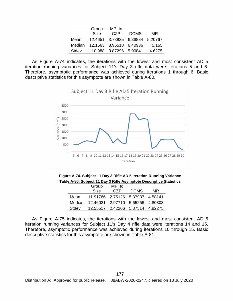
177 Distribution A: Approved for public release. 88ABW-2020-2247, cleared on 13 July 2020
Group Size
MPI to CZP DCMS MR
Mean 12.4651 3.78825 6.36834 5.20767 Median 12.1563 3.95518 6.40936 5.165 Stdev 10.988 3.87296 5.90841 4.6275
As Figure A-74 indicates, the iterations with the lowest and most consistent AD 5 iteration running variances for Subject 11’s Day 3 rifle data were iterations 5 and 6. Therefore, asymptotic performance was achieved during iterations 1 through 6. Basic descriptive statistics for this asymptote are shown in Table A-80.
Figure A-74. Subject 11 Day 3 Rifle AD 5 Iteration Running Variance Table A-80. Subject 11 Day 3 Rifle Asymptote Descriptive Statistics
Group Size
MPI to CZP DCMS MR
Mean 11.91766 2.75126 5.37937 4.58141 Median 12.46021 2.97710 5.65256 4.80303 Stdev 12.55517 2.42206 5.37514 4.82275
As Figure A-75 indicates, the iterations with the lowest and most consistent AD 5 iteration running variances for Subject 11’s Day 4 rifle data were iterations 14 and 15. Therefore, asymptotic performance was achieved during iterations 10 through 15. Basic descriptive statistics for this asymptote are shown in Table A-81.
0
500
1000
1500
2000
2500
3000
3500
5 6 7 8 9 10 11 12 13 14 15 16 17 18 19 20 21 22 23 24 25 26 27 28 29 30
Varia
nce
(cm
2 )
Iteration
Subject 11 Day 3 Rifle AD 5 Iteration Running Variance

178 Distribution A: Approved for public release. 88ABW-2020-2247, cleared on 13 July 2020
Figure A-75. Subject 11 Day 4 Rifle AD 5 Iteration Running Variance Table A-81. Subject 11 Day 4 Rifle Asymptote Descriptive Statistics
Group Size
MPI to CZP DCMS MR
Mean 13.53679 4.06425 6.57191 5.31965 Median 13.82902 4.31737 6.74133 5.43480 Stdev 13.54917 4.47249 6.7745 5.37368
As Figure A-76 indicates, the iterations with the lowest and most consistent AD 5 iteration running variances for Subject 11’s Day 5 rifle data were iterations 28 and 29. Therefore, asymptotic performance was achieved during iterations 24 through 29. Basic descriptive statistics for this asymptote are shown in Table A-82.
0100020003000400050006000700080009000
10000
5 6 7 8 9 10 11 12 13 14 15 16 17 18 19 20 21 22 23 24 25 26 27 28 29 30
Varia
nce
(cm
2 )
Iteration
Subject 11 Day 4 Rifle AD 5 Iteration Running Variance

179 Distribution A: Approved for public release. 88ABW-2020-2247, cleared on 13 July 2020
Figure A-76. Subject 11 Day 5 Rifle AD 5 Iteration Running Variance Table A-82. Subject 11 Day 5 Rifle Asymptote Descriptive Statistics
Group Size
MPI to CZP DCMS MR
Mean 9.10589 2.89864 4.61395 3.46209 Median 9.76041 3.10308 4.97515 3.72107 Stdev 10.1848 3.17526 5.14109 3.86039
As Table A-83 indicates, the null hypothesis of normality was not rejected for Subject 11’s rifle group size data. The boxplot in Figure A-77 does not, however, support a normal distribution. When Bartlett’s Test was performed on these data, the resulting K2 was 4.1682 and the p-value was 0.2439, which failed to reject the null hypothesis of homoscedasticity. The Kruskal-Wallis Test yielded a Χ2 value of 4.2302 and a p-value of 0.2377, thus failing to reject the null hypothesis of equality of dataset medians. As such, the analysis does not provide evidence of a change in group size during days 2-5.
Table A-83. Subject 11 Rifle Group Size Shapiro-Wilk Test Results Day W P-Value
2 0.8784599 0.2620592 3 0.8726064 0.2367936 4 0.9629918 0.8424755 5 0.9518377 0.7551357
0
2000
4000
6000
8000
10000
12000
5 6 7 8 9 10 11 12 13 14 15 16 17 18 19 20 21 22 23 24 25 26 27 28 29 30
Varia
nce
(cm
2 )
Iteration
Subject 11 Day 5 Rifle AD 5 Iteration Running Variance

180 Distribution A: Approved for public release. 88ABW-2020-2247, cleared on 13 July 2020
Figure A-77. Subject 11 Rifle Group Size Data
As Table A-84 indicates, the null hypothesis of normality was not rejected for Subject 11’s rifle MPI to CZP distance data. The boxplot in Figure A-78 does not, however, support a normal distribution. When Bartlett’s Test was performed on these data, the resulting K2 was 2.2141 and the p-value was 0.5292, which failed to reject the null hypothesis of homoscedasticity. The Kruskal-Wallis Test yielded a Χ2 value of 2.58 and a p-value of 0.461 thus failing to reject the null hypothesis of equality of dataset medians. As such, the analysis does not provide evidence of a change in MPI to CZP distance during days 2-5.
Table A-84. Subject 11 Rifle MPI to CZP Distance Shapiro-Wilk Test Results Day W P-Value
2 0.9046271 0.4020024 3 0.9584172 0.8074622 4 0.8632732 0.2006818 5 0.9152376 0.4717391

181 Distribution A: Approved for public release. 88ABW-2020-2247, cleared on 13 July 2020
Figure A-78. Subject 11 Rifle MPI to CZP Distance Data
As Table A-85 indicates, the null hypothesis of normality was not rejected for Subject 11’s rifle DCMS data. The boxplot in Figure A-79 does not, however, support a normal distribution. When Bartlett’s Test was performed on these data, the resulting K2 was 4.6871 and the p-value was 0.1962, which failed to reject the null hypothesis of homoscedasticity. The Kruskal-Wallis Test yielded a Χ2 value of 3.3867 and a p-value of 0.3358, thus failing to reject the null hypothesis of equality of dataset medians. As such, the analysis does not provide evidence of a change in DCMS during days 2-5.
Table A-85. Subject 11 Rifle DCMS Shapiro-Wilk Test Results Day W P-Value
2 0.8663433 0.2120140 3 0.9620732 0.8355676 4 0.9434074 0.6867562 5 0.9038350 0.3970943

182 Distribution A: Approved for public release. 88ABW-2020-2247, cleared on 13 July 2020
Figure A-79. Subject 11 Rifle DCMS Data
As Table A-86 indicates, the null hypothesis of normality was not rejected for Subject 11’s rifle mean radius data. The boxplot in Figure A-80 does not, however, support a normal distribution. When Bartlett’s Test was performed on these data, the resulting K2 was 5.1969 and the p-value was 0.1579, which failed to reject the null hypothesis of homoscedasticity. The Kruskal-Wallis Test yielded a Χ2 value of 5.9267 and a p-value of 0.1152, thus failing to reject the null hypothesis of equality of dataset medians. As such, the analysis does not provide evidence of a change in mean radius during days 2-5.
Table A-86. Subject 11 Rifle Mean Radius Shapiro-Wilk Test Results Day W P-Value
2 0.8182026 0.0851422 3 0.9411293 0.6683108 4 0.9310219 0.5880162 5 0.9730923 0.9125258

183 Distribution A: Approved for public release. 88ABW-2020-2247, cleared on 13 July 2020
Figure A-80. Subject 11 Rifle Mean Radius Data
6.11 Subject 12 Pistol Data
As Figure A-81 indicates, the iterations with the lowest and most consistent AD 5 iteration running variances for Subject 12’s Day 2 pistol data were iterations 5 and 6. Therefore, asymptotic performance was achieved during iterations 2 through 7. Basic descriptive statistics for this asymptote are shown in Table A-87.
Figure A-81. Subject 12 Day 2 Pistol AD 5 Iteration Running Variance
Table A-87. Subject 12 Day 2 Pistol Asymptote Descriptive Statistics
0
200
400
600
800
1000
1200
1400
1600
5 6 7 8 9 10 11 12 13 14 15 16 17 18 19 20 21 22 23 24 25 26 27 28 29 30
Varia
nce
(cm
2 )
Iteration
Subject 12 Day 2 Pistol AD 5 Iteration Running Variance

184 Distribution A: Approved for public release. 88ABW-2020-2247, cleared on 13 July 2020
Group Size
MPI to CZP DCMS MR
Mean 11.46206 4.52751 6.31355 4.50411 Median 11.4944 4.41306 6.45308 4.49330 Stdev 2.055605 2.26867 1.96834 0.745362
As Figure A-82 indicates, the iterations with the lowest and most consistent AD 5 iteration running variances for Subject 12’s Day 3 pistol data were iterations 24 and 25. Therefore, asymptotic performance was achieved during iterations 20 through 25. Basic descriptive statistics for this asymptote are shown in Table A-88.
Figure A-82. Subject 12 Day 3 Pistol AD 5 Iteration Running Variance Table A-88. Subject 12 Day 3 Pistol Asymptote Descriptive Statistics
Group Size
MPI to CZP DCMS MR
Mean 7.21407 1.75719 3.20431 2.85102 Median 6.78011 1.82423 3.17843 2.70711 Stdev 2.64131 0.57739 0.72781 0.93526
As Figure A-83 indicates, the iterations with the lowest and most consistent AD 5 iteration running variances for Subject 12’s Day 4 pistol data were iterations 12 and 13. Therefore, asymptotic performance was achieved during iterations 8 through 13. Basic descriptive statistics for this asymptote are shown in Table A-89.
0
100
200
300
400
500
600
700
5 6 7 8 9 10 11 12 13 14 15 16 17 18 19 20 21 22 23 24 25 26 27 28 29 30
Varia
nce
(cm
2 )
Iteration
Subject 12 Day 3 Pistol AD 5 Iteration Running Variance

185 Distribution A: Approved for public release. 88ABW-2020-2247, cleared on 13 July 2020
Figure A-83. Subject 12 Day 4 Pistol AD 5 Iteration Running Variance Table A-89. Subject 12 Day 4 Pistol Asymptote Descriptive Statistics
Group Size
MPI to CZP DCMS MR
Mean 7.73968 3.08062 4.52472 3.21211 Median 7.58259 2.57267 4.10526 3.12088 Stdev 2.04372 1.55789 1.58895 0.98603
As Figure A-84 indicates, the iterations with the lowest and most consistent AD 5 iteration running variances for Subject 12’s Day 5 pistol data were iterations 14 and 15. Therefore, asymptotic performance was achieved during iterations 10 through 15. Basic descriptive statistics for this asymptote are shown in Table A-90.
0
200
400
600
800
1000
1200
1400
5 6 7 8 9 10 11 12 13 14 15 16 17 18 19 20 21 22 23 24 25 26 27 28 29 30
Varia
nce
(cm
2 )
Iteration
Subject 12 Day 4 Pistol AD 5 Iteration Running Variance

186 Distribution A: Approved for public release. 88ABW-2020-2247, cleared on 13 July 2020
Figure A-84. Subject 12 Day 5 Pistol AD 5 Iteration Running Variance Table A-90. Subject 12 Day 5 Pistol Asymptote Descriptive Statistics
Group Size
MPI to CZP DCMS MR
Mean 5.18809 2.33313 3.10707 2.00586 Median 4.98697 2.15959 2.99439 1.95267 Stdev 1.18424 1.13367 1.06745 0.40397
As Table A-91 indicates, the null hypothesis of normality was not rejected for Subject 12’s pistol group size data. The boxplot in Figure A-85 does not, however, support a normal distribution. When Bartlett’s Test was performed on these data, the resulting K2 was 4.7574 and the p-value was 0.1905, which failed to reject the null hypothesis of homoscedasticity. The Kruskal-Wallis Test yielded a Χ2 value of 13.771 and a p-value of 0.003234, thus rejecting the null hypothesis of equality of dataset medians.
Table A-91. Subject 12 Pistol Group Size Shapiro-Wilk Test Results Day W P-Value
2 0.926223 0.519251 3 0.961259 0.829459 4 0.880475 0.228567 5 0.917231 0.448194
0
2000
4000
6000
8000
10000
12000
5 6 7 8 9 10 11 12 13 14 15 16 17 18 19 20 21 22 23 24 25 26 27 28 29 30
Varia
nce
(cm
2 )
Iteration
Subject 12 Day 5 Pistol AD 5 Iteration Running Variance

187 Distribution A: Approved for public release. 88ABW-2020-2247, cleared on 13 July 2020
Figure A-85. Subject 12 Pistol Group Size
As Table A-92 indicates, the only statistically significant difference was between Subject 12’s day 2 and day 5 pistol group sizes. While the difference is statistically significant, it is not indicative of a trend, as there is not a statistically significant difference between days 3 and 4.
Table A-92. Subject 12 Pistol Group Size Dunn's Test Results Days Z P-Value 2 & 3 2.274294 0.0344 2 & 4 1.559515 0.0892 2 & 5 3.63887 0.0008 3 & 4 0.714778 0.2374 3 & 5 1.364576 0.1034 4 & 5 2.079354 0.0376
As Table A-93 indicates, the null hypothesis of normality was not rejected for Subject 12’s MPI to CZP distance data. The boxplot in Figure A-86 does not, however, support a normal distribution. When Bartlett’s Test was performed on these data, the resulting K2 was 8.5619 and the p-value was 0.03572, which rejected the null hypothesis of homoscedasticity. The Brunner-Dette-Munk test yielded an F value of 2.641306 and a p-value of 0.0833049, thus rejecting the null hypothesis of equality of distribution functions. As such, the analysis does not provide evidence of a change in MPI to CZP distance during days 2-5.
Table A-93. Subject 12 Pistol MPI to CZP Distance Shapiro-Wilk Test Results

188 Distribution A: Approved for public release. 88ABW-2020-2247, cleared on 13 July 2020
Day W P-Value 2 0.920141 0.470489 3 0.941438 0.651708 4 0.876989 0.213417 5 0.948686 0.717721
Figure A-86. Subject 12 Pistol MPI to CZP Distance
As Table A-94 indicates, the null hypothesis of normality was not rejected for Subject 12’s pistol DCMS data. The boxplot in Figure A-87 does not, however, support a normal distribution. When Bartlett’s Test was performed on these data, the resulting K2 was 5.4985 and the p-value was 0.1387, which failed to reject the null hypothesis of homoscedasticity. The Kruskal-Wallis Test yielded a Χ2 value of 12.399 and a p-value of 0.006134, thus rejecting the null hypothesis of equality of dataset medians.
Table A-94. Subject 12 Pistol DCMS Shapiro-Wilk Test Results Day W P-Value
2 0.895809 0.306353 3 0.978311 0.950947 4 0.953601 0.762319 5 0.959463 0.814116

189 Distribution A: Approved for public release. 88ABW-2020-2247, cleared on 13 July 2020
Figure A-87. Subject 12 Pistol DCMS Data
As indicated in Table A-95, the only statistically significant differences in Subject 12’s pistol DCMS data are between days 2 and 3 and days 2 and 5. These results imply that day 2’s DCMS was greater than that of 3 or 5, but do not necessarily imply a trend.
Table A-95. Subject 12 Pistol DCMS Dunn's Test Results Days Z P-Value 2 & 3 3.086542 0.0061 2 & 4 1.299596 0.1162 2 & 5 2.826622 0.0071 3 & 4 1.786945 0.0739 3 & 5 0.259919 0.3975 4 & 5 1.527026 0.0951
As Table A-96 indicates, the null hypothesis of normality was not rejected for Subject 12’s pistol mean radius data. The boxplot in Figure A-88 does not, however, support a normal distribution. When Bartlett’s Test was performed on these data, the resulting K2 was 5.6126 and the p-value was 0.1321, which failed to reject the null hypothesis of homoscedasticity. The Kruskal-Wallis Test yielded a Χ2 value of 14.552 and a p-value of 0.002242, thus rejecting the null hypothesis of equality of dataset medians.
Table A-96. Subject 12 Pistol Mean Radius Shapiro-Wilk Test Results Day W P-Value

190 Distribution A: Approved for public release. 88ABW-2020-2247, cleared on 13 July 2020
2 0.959619 0.815459 3 0.920784 0.475507 4 0.839415 0.098117 5 0.966668 0.873471
Figure A-88. Subject 12 Pistol Mean Radius Data
As Table A-97 indicates, the only statistically significant difference in Subject 12’s pistol mean radius data is between days 2 and 5.
Table A-97. Subject 12 Pistol Mean Radius Dunn's Test Results Days Z P-Value 2 & 3 2.111844 0.0347 2 & 4 1.364576 0.1034 2 & 5 3.73634 0.0006 3 & 4 0.747268 0.2275 3 & 5 1.624495 0.0782 4 & 5 2.371763 0.0266
6.12 Subject 12 Rifle Data
As Figure A-89 indicates, the iterations with the lowest and most consistent AD 5 iteration running variances for Subject 12’s Day 2 rifle data were iterations 18 and 19. Therefore, asymptotic performance was achieved during iterations 14 through 19. Basic descriptive statistics for this asymptote are shown in Table A-98.
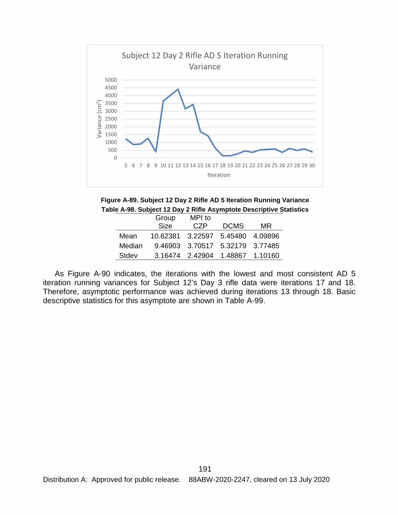
191 Distribution A: Approved for public release. 88ABW-2020-2247, cleared on 13 July 2020
Figure A-89. Subject 12 Day 2 Rifle AD 5 Iteration Running Variance Table A-98. Subject 12 Day 2 Rifle Asymptote Descriptive Statistics
Group Size
MPI to CZP DCMS MR
Mean 10.62381 3.22597 5.45480 4.09896 Median 9.46903 3.70517 5.32179 3.77485 Stdev 3.16474 2.42904 1.48867 1.10160
As Figure A-90 indicates, the iterations with the lowest and most consistent AD 5 iteration running variances for Subject 12’s Day 3 rifle data were iterations 17 and 18. Therefore, asymptotic performance was achieved during iterations 13 through 18. Basic descriptive statistics for this asymptote are shown in Table A-99.
0500
100015002000250030003500400045005000
5 6 7 8 9 10 11 12 13 14 15 16 17 18 19 20 21 22 23 24 25 26 27 28 29 30
Varia
nce
(cm
2 )
Iteration
Subject 12 Day 2 Rifle AD 5 Iteration Running Variance

192 Distribution A: Approved for public release. 88ABW-2020-2247, cleared on 13 July 2020
Figure A-90. Subject 12 Day 3 Rifle AD 5 Iteration Running Variance Table A-99. Subject 12 Day 3 Rifle Asymptote Descriptive Statistics
Group Size
MPI to CZP DCMS MR
Mean 11.00041 4.29972 6.12184 4.00236 Median 11.28481 4.38704 5.91103 4.20631 Stdev 2.74123 2.09810 1.35194 0.82185
As Figure A-91 indicates, the iterations with the lowest and most consistent AD 5 iteration running variances for Subject 12’s Day 4 rifle data were iterations 16 and 17. Therefore, asymptotic performance was achieved during iterations 12 through 17. Basic descriptive statistics for this asymptote are shown in Table A-100.
0
1000
2000
3000
4000
5000
6000
7000
5 6 7 8 9 10 11 12 13 14 15 16 17 18 19 20 21 22 23 24 25 26 27 28 29 30
Varia
nce
(cm
2 )
Iteration
Subject 12 Day 3 Rifle AD 5 Iteration Running Variance

193 Distribution A: Approved for public release. 88ABW-2020-2247, cleared on 13 July 2020
Figure A-91. Subject 12 Day 4 Rifle AD 5 Iteration Running Variance Table A-100. Subject 12 Day 4 Rifle Asymptote Descriptive Statistics
Group Size
MPI to CZP DCMS MR
Mean 11.22525 4.30128 5.99900 4.63699 Median 11.50244 3.58660 6.36189 4.65920 Stdev 2.84439 2.10056 1.54132 1.12990
As Figure A-92 indicates, the iterations with the lowest and most consistent AD 5 iteration running variances for Subject 12’s Day 5 rifle data were iterations 7 and 8. Therefore, asymptotic performance was achieved during iterations 3 through 8. Basic descriptive statistics for this asymptote are shown in Table A-101.
0
1000
2000
3000
4000
5000
6000
7000
5 6 7 8 9 10 11 12 13 14 15 16 17 18 19 20 21 22 23 24 25 26 27 28 29 30
Varia
nce
(cm
2 )
Iteration
Subject 12 Day 4 Rifle AD 5 Iteration Running Variance

194 Distribution A: Approved for public release. 88ABW-2020-2247, cleared on 13 July 2020
Figure A-92. Subject 12 Day 5 Rifle AD 5 Iteration Running Variance Table A-101. Subject 12 Day 5 Rifle Asymptote Descriptive Statistics
Group Size
MPI to CZP DCMS MR
Mean 10.56052 4.22686 5.75580 4.22095 Median 11.05873 4.27478 6.09339 4.28571 Stdev 1.59644 1.30330 1.24918 0.52811
As Table A-102 indicates, the null hypothesis of normality was not rejected for Subject 12’s rifle group size data. The boxplot in Figure A-93 does not, however, support a normal distribution. When Bartlett’s Test was performed on these data, the resulting K2 was 2.3681 and the p-value was 0.4996, which failed to reject the null hypothesis of homoscedasticity. The Kruskal-Wallis Test yielded a Χ2 value of 1.9866 and a p-value of 0.5722, thus failing to reject the null hypothesis of equality of dataset medians. As such, the analysis provides no evidence of a change in group size during days 2-5.
Table A-102. Subject 12 Rifle Group Size Shapiro-Wilk Test Results Day W P-Value
2 0.877552 0.2158 3 0.993422 0.997901 4 0.947699 0.708719 5 0.880901 0.23048
0
200
400
600
800
1000
1200
5 6 7 8 9 10 11 12 13 14 15 16 17 18 19 20 21 22 23 24 25 26 27 28 29 30
Varia
nce
(cm
2 )
Iteration
Subject 12 Day 5 Rifle AD 5 Iteration Running Variance

195 Distribution A: Approved for public release. 88ABW-2020-2247, cleared on 13 July 2020
Figure A-93. Subject 12 Rifle Group Size Data
As Table A-103 indicates, the null hypothesis of normality was not rejected for Subject 12’s rifle MPI to CZP distance data. The boxplot in Figure A-94 does not, however, support a normal distribution. When Bartlett’s Test was performed on these data, the resulting K2 was 0.5 and the p-value was 0.9189, which failed to reject the null hypothesis of homoscedasticity. The Kruskal-Wallis Test yielded a Χ2 value of 0.74 and a p-value of 0.8638, thus failing to reject the null hypothesis of equality of dataset medians. As such, the analysis provides no evidence of a change in MPI to CZP distance during days 2-5.
Table A-103. Subject 12 Rifle MPI to CZP Distance Shapiro-Wilk Test Results Day W P-Value
2 0.909011 0.389068 3 0.944948 0.683608 4 0.86931 0.183063 5 0.94738 0.705804
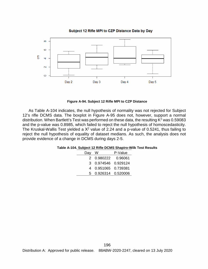
196 Distribution A: Approved for public release. 88ABW-2020-2247, cleared on 13 July 2020
Figure A-94. Subject 12 Rifle MPI to CZP Distance
As Table A-104 indicates, the null hypothesis of normality was not rejected for Subject 12’s rifle DCMS data. The boxplot in Figure A-95 does not, however, support a normal distribution. When Bartlett’s Test was performed on these data, the resulting K2 was 0.59083 and the p-value was 0.8985, which failed to reject the null hypothesis of homoscedasticity. The Kruskal-Wallis Test yielded a Χ2 value of 2.24 and a p-value of 0.5241, thus failing to reject the null hypothesis of equality of dataset medians. As such, the analysis does not provide evidence of a change in DCMS during days 2-5.
Table A-104. Subject 12 Rifle DCMS Shapiro-Wilk Test Results Day W P-Value
2 0.980222 0.96061 3 0.974546 0.929124 4 0.951065 0.739381 5 0.926314 0.520006
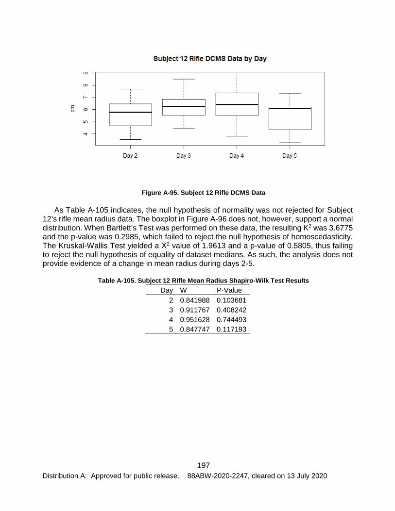
197 Distribution A: Approved for public release. 88ABW-2020-2247, cleared on 13 July 2020
Figure A-95. Subject 12 Rifle DCMS Data
As Table A-105 indicates, the null hypothesis of normality was not rejected for Subject 12’s rifle mean radius data. The boxplot in Figure A-96 does not, however, support a normal distribution. When Bartlett’s Test was performed on these data, the resulting K2 was 3.6775 and the p-value was 0.2985, which failed to reject the null hypothesis of homoscedasticity. The Kruskal-Wallis Test yielded a Χ2 value of 1.9613 and a p-value of 0.5805, thus failing to reject the null hypothesis of equality of dataset medians. As such, the analysis does not provide evidence of a change in mean radius during days 2-5.
Table A-105. Subject 12 Rifle Mean Radius Shapiro-Wilk Test Results Day W P-Value
2 0.841988 0.103681 3 0.911767 0.408242 4 0.951628 0.744493 5 0.847747 0.117193

198 Distribution A: Approved for public release. 88ABW-2020-2247, cleared on 13 July 2020
Figure A-96. Subject 12 Rifle Mean Radius Data

199 Distribution A: Approved for public release. 88ABW-2020-2247, cleared on 13 July 2020
APPENDIX B
6.1 Subject CSA02 Results 6.1.1 IES Scoring Results
As Figure B-1 indicates, when correct response radii were 5 and 4 cm, based on MPI to CZP distance calculations, the trends were similar. Significant changes occurred when radii were reduced to 3 and 2 cm. At a radius of 3 cm, Subject CSA02 showed a decrease in IES on day 4, followed by a large increase on day 5. At a radius of 2 cm, however, the trend is reversed with a large increase on day 4 followed by a large decrease on day 5.
Figure B-1. Subject CSA02 IES - MPI to CZP Distance Based
As Figure B-2 indicates, MPI to CZP distance based RT showed a similar trend for radii ranging from 5 to 3 cm. At a radius of 2 cm, however, there is a dramatic change on day 5 where the RT value was 0 because no shot groups were observed within a 2 cm radius of the center of the target.
0
20
40
60
80
100
120
140
160
180
200
Day 2 Day 3 Day 4 Day 5
IES
CSA02 IES - MPI to CZP Distance Based
5cm
4cm
3cm
2cm

200 Distribution A: Approved for public release. 88ABW-2020-2247, cleared on 13 July 2020
Figure B-2. Subject CSA02 RT - MPI to CZP Distance Based
As Figure B-3 indicates, the larger radii resulted in larger proportions of hits during each day of firing. At a radius of 4 cm three was an improvement from day 2 to day 4 of firing, while at a radius of 3 cm there was an improvement from day 3 to day 4. Overall, however, the most noteworthy trend was the large decline in performance on day 5 of firing.
Figure B-3. Subject CSA02 Proportion Correct - MPI to CZP Distance Based
When IES was calculated at multiple radii based on DCMS measurements, the trends for 5 and 4 cm radii were very similar, as shown in Figure B-4. The overall 3 cm trend showed slightly higher overall scores and a slight decrease on day 4 of firing. The 2 cm trend, however, was markedly different in both overall IES value and the trend, which was
0
1
2
3
4
5
6
7
Day 2 Day 3 Day 4 Day 5
RT (s
)
CSA02 RT - MPI to CZP Distance Based
5 cm
4 cm
3 cm
2 cm
0
0.1
0.2
0.3
0.4
0.5
0.6
0.7
0.8
0.9
Day 2 Day 3 Day 4 Day 5
Prop
ortio
n Co
rrec
t
CSA02 Proportion Correct - MPI to CZP Distance Based
5 cm
4 cm
3 cm
2 cm

201 Distribution A: Approved for public release. 88ABW-2020-2247, cleared on 13 July 2020
relatively constant from day 2 to day 3, but increased on day 4 before drastically decreasing on day 5.
Figure B-4. Subject CSA02 IES - DCMS Based
An examination of trends in DCMS based RT values, as shown in Figure B-5, indicates highly similar results for radii from 5 to 3 cm, with an increase on day 4 followed by a significant decrease on day 5. This decrease was due to the fact that the no shot groups fell within the 2 cm radius on that day of firing.
Figure B-5. Subject CSA02 RT – DCMS Based
0
20
40
60
80
100
120
140
160
180
200
Day 2 Day 3 Day 4 Day 5
IES
CSA02 IES - DCMS Based
5cm
4cm
3cm
2cm
0
1
2
3
4
5
6
7
Day 2 Day 3 Day 4 Day 5
RT (s
)
CSA02 RT - DCMS Based
5 cm
4 cm
3 cm
2 cm

202 Distribution A: Approved for public release. 88ABW-2020-2247, cleared on 13 July 2020
The DCMS based proportion correct results, as shown in Figure B-6, follow the expected trend of greater value with greater radius. Each radius, however, follows a slightly different trend from day to day, with 5 cm showing a slight decrease from day 2 to day 3, but 4 and 3 cm showing increases while 2 cm remains relatively stable. Overall, proportion correct showed an improvement from day 2 to day 5 only for a radius of 5 cm.
Figure B-6. Subject CSA02 Proportion Correct - DCMS Based
6.1.2 Conditional Accuracy Function Results
As Table B-1 indicates, the null hypothesis of a normal distribution was rejected for some quantiles. The boxplot in Figure B-7 does not provide information to the contrary. Bartlett’s test produced a K2 value of 8.5268 and a p value of 0.07408, failing to reject the null hypothesis of homoscedasticity. The Kruskal-Wallis test produced a Χ2 value of 0.43011 and a p value of 0.9799, failing to reject the null hypothesis of equality of dataset medians. Because this null hypothesis was not rejected, it cannot be concluded that accuracy, as measured by 1/MPI to CZP distance, differed by time quantile on day 2.
Table B-1. Subject CSA02 Day 2 Five Quantile 1/MPI to CZP Distance Shapiro-Wilk Test Results Quantile W P-Value
1 0.9314 0.5907 2 0.9164 0.4801 3 0.654 0.002 4 0.8258 0.0989 5 0.6853 0.0043
0
0.1
0.2
0.3
0.4
0.5
0.6
0.7
0.8
0.9
Day 2 Day 3 Day 4 Day 5
Prop
ortio
n Co
rrec
t
CSA02 Proportion Correct - DCMS Based
5 cm
4 cm
3 cm
2 cm
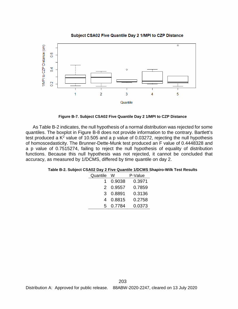
203 Distribution A: Approved for public release. 88ABW-2020-2247, cleared on 13 July 2020
Figure B-7. Subject CSA02 Five Quantile Day 2 1/MPI to CZP Distance
As Table B-2 indicates, the null hypothesis of a normal distribution was rejected for some quantiles. The boxplot in Figure B-8 does not provide information to the contrary. Bartlett’s test produced a K2 value of 10.505 and a p value of 0.03272, rejecting the null hypothesis of homoscedasticity. The Brunner-Dette-Munk test produced an F value of 0.4448328 and a p value of 0.7515274, failing to reject the null hypothesis of equality of distribution functions. Because this null hypothesis was not rejected, it cannot be concluded that accuracy, as measured by 1/DCMS, differed by time quantile on day 2.
Table B-2. Subject CSA02 Day 2 Five Quantile 1/DCMS Shapiro-Wilk Test Results Quantile W P-Value
1 0.9038 0.3971 2 0.9557 0.7859 3 0.8891 0.3136 4 0.8815 0.2758 5 0.7784 0.0373

204 Distribution A: Approved for public release. 88ABW-2020-2247, cleared on 13 July 2020
Figure B-8. Subject CSA02 Five Quantile Day 2 1/DCMS
As Table B-3 indicates, the null hypothesis of a normal distribution was rejected for some quantiles. The boxplot in Figure B-9 does not provide information to the contrary. Bartlett’s test produced a K2 value of 11.646 and a p value of 0.02019, rejecting the null hypothesis of homoscedasticity. The Brunner-Dette-Munk test produced an F value of 1.336754 and a p value of 0.2935303, failing to reject the null hypothesis of equality of distribution functions. Because this null hypothesis was not rejected, it cannot be concluded that accuracy, as measured by 1/MPI to CZP distance, differed by time quantile on day 3.
Table B-3. Subject CSA02 Day 3 Five Quantile 1/MPI to CZP Distance Shapiro-Wilk Test Results Quantile W P-Value
1 0.8976 0.3601 2 0.7456 0.0181 3 0.6115 0.0006 4 0.685 0.0043 5 0.8648 0.2063

205 Distribution A: Approved for public release. 88ABW-2020-2247, cleared on 13 July 2020
Figure B-9. Subject CSA02 Five Quantile Day 3 1/MPI to CZP Distance
As Table B-4 indicates, the null hypothesis of a normal distribution was rejected for some quantiles. The boxplot in Figure B-10 does not provide information to the contrary. Bartlett’s test produced a K2 value of 2.0804 and a p value of 0.721, failing to reject the null hypothesis of homoscedasticity. The Kruskal-Wallis test produced a Χ2 value of 2.3097 and a p value of 0.679, failing to reject the null hypothesis of equality of dataset medians. Because this null hypothesis was not rejected, it cannot be concluded that accuracy, as measured by 1/DCMS, differed by time quantile on day 3.
Table B-4. Subject CSA02 Day 3 Five Quantile 1/DCMS Shapiro-Wilk Test Results Quantile W P-Value
1 0.7783 0.0371 2 0.7591 0.0244 3 0.7246 0.0111 4 0.9242 0.536 5 0.801 0.06

206 Distribution A: Approved for public release. 88ABW-2020-2247, cleared on 13 July 2020
Figure B-10. Subject CSA02 Five Quantile Day 3 1/DCMS
As Table B-5 indicates, the null hypothesis of a normal distribution was rejected for some quantiles. The boxplot in Figure B-11 does not provide information to the contrary. Bartlett’s test produced a K2 value of 35.103 and a p value of 4.424e-07, rejecting the null hypothesis of homoscedasticity. The Brunner-Dette-Munk test produced an F value of 2.127025 and a p value of 0.1187848, failing to reject the null hypothesis of equality of distribution functions. Because this null hypothesis was not rejected, it cannot be concluded that accuracy, as measured by 1/MPI to CZP distance, differed by time quantile on day 4.
Table B-5. Subject CSA02 Day 4 Five Quantile 1/MPI to CZP Distance Shapiro-Wilk Test Results Quantile W P-Value
1 0.9122 0.4513 2 0.9166 0.4811 3 0.9331 0.6042 4 0.6493 0.0017 5 0.9428 0.6815

207 Distribution A: Approved for public release. 88ABW-2020-2247, cleared on 13 July 2020
Figure B-11. Subject CSA02 Five Quantile Day 4 1/MPI to CZP Distance
As Table B-6 indicates, the null hypothesis of a normal distribution was not rejected for any quantiles. The boxplot in Figure B-12 is not, however, indicative of a normal distribution for all datasets. Bartlett’s test produced a K2 value of 2.8966 and a p value of 0.5753, failing to reject the null hypothesis of homoscedasticity. The Kruskal-Wallis test produced a Χ2 value of 9.8323 and a p value of 0.04335, rejecting the null hypothesis of equality of dataset medians. Because this null hypothesis was rejected, it can be concluded that accuracy, as measured by 1/DCMS, differed by time quantile on day 4.
Table B-6. Subject CSA02 Day 4 Five Quantile 1/DCMS Shapiro-Wilk Test Results Quantile W P-Value
1 0.9143 0.4655 2 0.9814 0.9581 3 0.8996 0.3716 4 0.8043 0.0643 5 0.9922 0.9939

208 Distribution A: Approved for public release. 88ABW-2020-2247, cleared on 13 July 2020
Figure B-12. Subject CSA02 Five Quantile Day 4 1/DCMS
As Table B-7 indicates, significant differences were found between quantiles 1 and 2; 1 and 5; and 4 and 5. These differences are not progressive, however, and do not appear to be indicative of a trend.
Table B-7. Subject CSA02 Day 4 Five Quantile 1/DCMS Dunn's Test Results Quantiles Z P-Value
1 & 2 -1.96748 0.0246 1 & 3 -1.1149 0.1324 1 & 4 -0.32791 0.3715 1 & 5 -2.65609 0.0040 2 & 3 0.852573 0.1969 2 & 4 1.639564 0.0505 2 & 5 -0.68862 0.2455 3 & 4 0.786991 0.2156 3 & 5 -1.54119 0.0616 4 & 5 -2.32818 0.0100
As Table B-8 indicates, the null hypothesis of a normal distribution was not rejected for any quantiles. The boxplot in Figure B-13 is not, however, indicative of a normal distribution for all datasets. Bartlett’s test produced a K2 value of 1.7437 and a p value of 0.7828, failing to reject the null hypothesis of homoscedasticity. The Kruskal-Wallis test produced a Χ2 value of 1.9542 and a p value of 0.7442, failing to reject the null hypothesis of equality of dataset medians. Because this null hypothesis was not rejected, it cannot be concluded that accuracy, as measured by 1/MPI to CZP distance, differed by time quantile on day 5.
Table B-8. Subject CSA02 Day 5 Five Quantile 1/MPI to CZP Distance Shapiro-Wilk Test Results Quantile W P-Value

209 Distribution A: Approved for public release. 88ABW-2020-2247, cleared on 13 July 2020
1 0.9421 0.6761 2 0.9797 0.9499 3 0.8994 0.3706 4 0.8928 0.3332 5 0.889 0.3128
Figure B-13. Subject CSA02 Five Quantile Day 5 1/MPI to CZP Distance
As Table B-9 indicates, the null hypothesis of a normal distribution was not rejected for any quantiles. The boxplot in Figure B-14 is not, however, indicative of a normal distribution for all datasets. Bartlett’s test produced a K2 value of 4.3976 and a p value of 0.3549, failing to reject the null hypothesis of homoscedasticity. The Kruskal-Wallis test produced a Χ2 value of 2.628 and a p value of 0.6219, failing to reject the null hypothesis of equality of dataset medians. Because this null hypothesis was not rejected, it cannot be concluded that accuracy, as measured by 1/DCMS, differed by time quantile on day 5.
Table B-9. Subject CSA02 Day 5 Five Quantile 1/DCMS Shapiro-Wilk Test Results Quantile W P-Value
1 0.9906 0.9906 2 0.9314 0.5912 3 0.9191 0.4986

210 Distribution A: Approved for public release. 88ABW-2020-2247, cleared on 13 July 2020
4 0.8933 0.3357 5 0.8681 0.2189
Figure B-14. Subject CSA02 Five Quantile Day 5 1/DCMS
As Table B-10 indicates, the null hypothesis of a normal distribution was rejected for some quantiles. The boxplot in Figure B-15 does not provide information to the contrary. Bartlett’s test produced a K2 value of 10.624 and a p value of 0.05936, failing to reject the null hypothesis of homoscedasticity. The Kruskal-Wallis test produced a Χ2 value of 2.8787 and a p value of 0.7187, failing to reject the null hypothesis of equality of dataset medians. Because this null hypothesis was not rejected, it cannot be concluded that accuracy, as measured by 1/MPI to CZP distance, differed by time quantile on day 2.
Table B-10. Subject CSA02 Day 2 Six Quantile 1/MPI to CZP Distance Shapiro-Wilk Test Results Quantile W P-Value
1 0.8957 0.3867 2 0.8849 0.3322 3 0.905 0.4381 4 0.7803 0.0555

211 Distribution A: Approved for public release. 88ABW-2020-2247, cleared on 13 July 2020
5 0.7133 0.0131 6 0.7374 0.0226
Figure B-15. Subject CSA02 Six Quantile Day 2 1/MPI to CZP Distance
As Table B-11 indicates, the null hypothesis of a normal distribution was not rejected for any quantiles. The boxplot in Figure B-16 is not, however, indicative of a normal distribution for all datasets. Bartlett’s test produced a K2 value of 10.606 and a p value of 0.05978, failing to reject the null hypothesis of homoscedasticity. The Kruskal-Wallis test produced a Χ2 value of 3.0387 and a p value of 0.694, failing to reject the null hypothesis of equality of dataset medians. Because this null hypothesis was not rejected, it cannot be concluded that accuracy, as measured by 1/DCMS, differed by time quantile on day 2.
Table B-11. Subject CSA02 Day 2 Six Quantile 1/DCMS Shapiro-Wilk Test Results Quantile W P-Value
1 0.9075 0.4525 2 0.952 0.7516 3 0.9698 0.8738 4 0.7947 0.0733 5 0.8744 0.2845 6 0.8346 0.1506

212 Distribution A: Approved for public release. 88ABW-2020-2247, cleared on 13 July 2020
Figure B-16. Subject CSA03 Six Quantile Day 2 1/DCMS
As Table B-12 indicates, the null hypothesis of a normal distribution was rejected for some quantiles. The boxplot in Figure B-17 is not, however, indicative of a normal distribution for all datasets. Bartlett’s test produced a K2 value of 12.866 and a p value of 0.02467, rejecting the null hypothesis of homoscedasticity. The Brunner-Dette-Munk test produced an F value of 1.10129 and a p value of 0.3821321, failing to reject the null hypothesis of equality of distribution functions. Because this null hypothesis was not rejected, it cannot be concluded that accuracy, as measured by 1/MPI to CZP distance, differed by time quantile on day 3.
Table B-12. Subject CSA02 Day 3 Six Quantile 1/MPI to CZP Distance Shapiro-Wilk Test Results Quantile W P-Value
1 0.9709 0.8807 2 0.922 0.543 3 0.8027 0.0853 4 0.6596 0.0035 5 0.8024 0.0847 6 0.825 0.1276

213 Distribution A: Approved for public release. 88ABW-2020-2247, cleared on 13 July 2020
Figure B-17. Subject CSA02 Six Quantile Day 3 1/MPI to CZP Distance
As Table B-13 indicates, the null hypothesis of a normal distribution was rejected for some quantiles. The boxplot in Figure B-18 does not provide information to the contrary. Bartlett’s test produced a K2 value of 2.2291 and a p value of 0.8166, failing to reject the null hypothesis of homoscedasticity. The Kruskal-Wallis test produced a Χ2 value of 2.7342 and a p value of 0.7409, failing to reject the null hypothesis of equality of dataset medians. Because this null hypothesis was not rejected, it cannot be concluded that accuracy, as measured by 1/DCMS, differed by time quantile on day 3.
Table B-13. Subject CSA02 Day 3 Six Quantile 1/DCMS Shapiro-Wilk Test Results Quantile W P-Value
1 0.8907 0.3605 2 0.8596 0.2267 3 0.8347 0.1509 4 0.7018 0.01 5 0.8884 0.3493 6 0.7709 0.046

214 Distribution A: Approved for public release. 88ABW-2020-2247, cleared on 13 July 2020
Figure B-18. Subject CSA02 Six Quantile Day 3 1/DCMS
As Table B-14 indicates, the null hypothesis of a normal distribution was rejected for some quantiles. The boxplot in Figure B-19 does not provide information to the contrary. Bartlett’s test produced a K2 value of 28.941 and a p value of 2.382e-05, rejecting the null hypothesis of homoscedasticity. The Brunner-Dette-Munk test produced an F value of 3.212478 and a p value of 0.03385637, rejecting the null hypothesis of equality of distribution functions. Because this null hypothesis was rejected, it can be concluded that accuracy, as measured by 1/MPI to CZP distance, differed by time quantile on day 4.
Table B-14. Subject CSA02 Day 4 Six Quantile 1/MPI to CZP Distance Shapiro-Wilk Test Results Quantile W P-Value
1 0.974992 0.906219 2 0.966978 0.855524 3 0.897938 0.398592 4 0.91024 0.469036 5 0.582943 0.000367 6 0.965864 0.848103
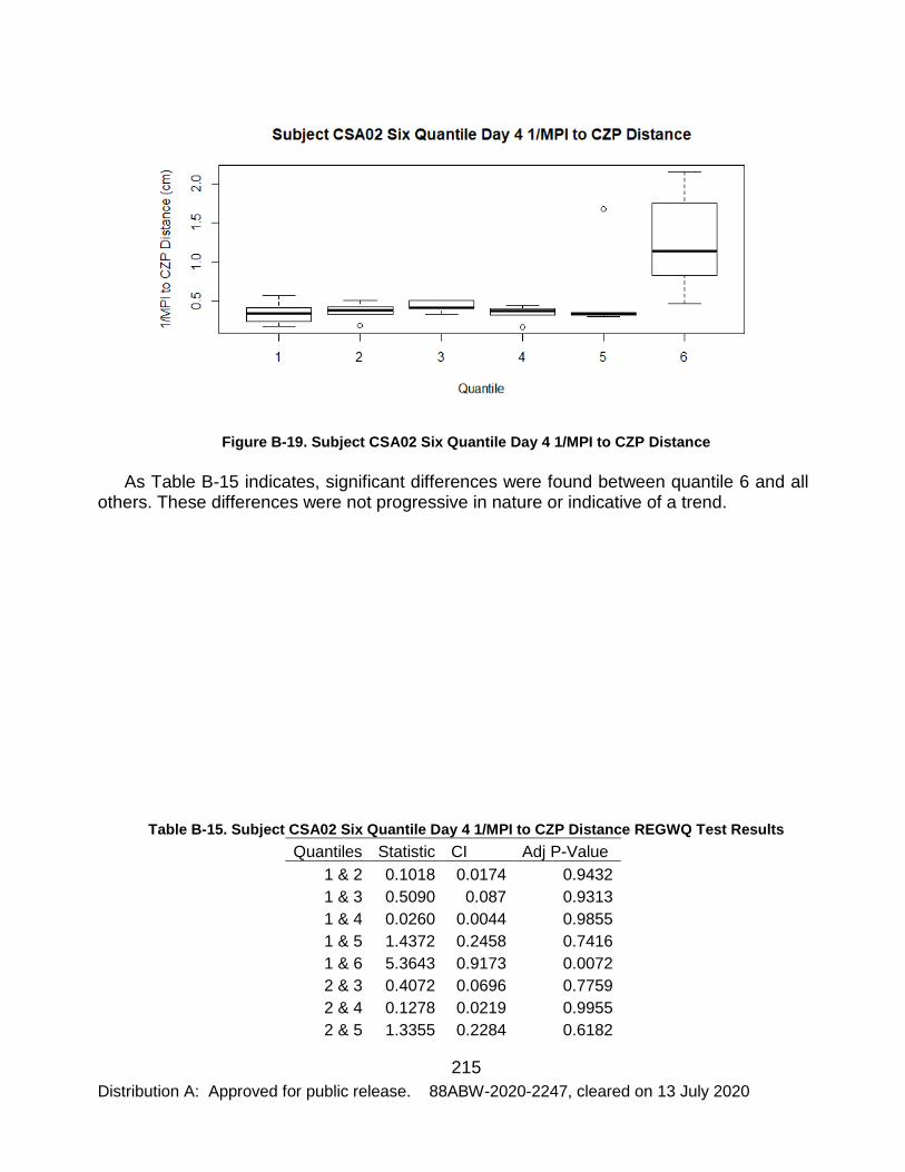
215 Distribution A: Approved for public release. 88ABW-2020-2247, cleared on 13 July 2020
Figure B-19. Subject CSA02 Six Quantile Day 4 1/MPI to CZP Distance
As Table B-15 indicates, significant differences were found between quantile 6 and all others. These differences were not progressive in nature or indicative of a trend.
Table B-15. Subject CSA02 Six Quantile Day 4 1/MPI to CZP Distance REGWQ Test Results Quantiles Statistic CI Adj P-Value
1 & 2 0.1018 0.0174 0.9432 1 & 3 0.5090 0.087 0.9313 1 & 4 0.0260 0.0044 0.9855 1 & 5 1.4372 0.2458 0.7416 1 & 6 5.3643 0.9173 0.0072 2 & 3 0.4072 0.0696 0.7759 2 & 4 0.1278 0.0219 0.9955 2 & 5 1.3355 0.2284 0.6182

216 Distribution A: Approved for public release. 88ABW-2020-2247, cleared on 13 July 2020
2 & 6 5.2625 0.8999 0.0055 3 & 4 0.5350 0.0915 0.9811 3 & 5 0.9282 0.1587 0.5179
3 & 6 4.8553 0.8303 0.0059 4 & 5 1.4632 0.2502 0.8368 4 & 6 5.3903 0.9218 0.0097 5 & 6 3.9270 0.6716 0.0105
As Table B-16 indicates, the null hypothesis of a normal distribution was rejected for some quantiles. The boxplot in Figure B-20 does not provide information to the contrary. Bartlett’s test produced a K2 value of 3.4961 and a p value of 0.624, failing to reject the null hypothesis of homoscedasticity. The Kruskal-Wallis test produced a Χ2 value of 9.031 and a p value of 0.1078, failing to reject the null hypothesis of equality of dataset medians. Because this null hypothesis was not rejected, it cannot be concluded that accuracy, as measured by 1/DCMS, differed by time quantile on day 4.
Table B-16. Subject CSA02 Day 4 Six Quantile 1/DCMS Shapiro-Wilk Test Results Quantile W P-Value
1 0.8907 0.3605 2 0.8596 0.2267 3 0.8347 0.1509 4 0.7018 0.01 5 0.8884 0.3493 6 0.7709 0.046
Figure B-20. Subject CSA02 Six Quantile Day 4 1/DCMS
As Table B-17 indicates, the null hypothesis of a normal distribution was not rejected for any quantiles. The boxplot in Figure B-21 is not, however, indicative of a normal distribution

217 Distribution A: Approved for public release. 88ABW-2020-2247, cleared on 13 July 2020
for all datasets. Bartlett’s test produced a K2 value of 2.909 and a p value of 0.714, failing to reject the null hypothesis of homoscedasticity. The Kruskal-Wallis test produced a Χ2 value of 3.3685 and a p value of 0.6434, failing to reject the null hypothesis of equality of dataset medians. Because this null hypothesis was not rejected, it cannot be concluded that accuracy, as measured by 1/MPI to CZP distance, differed by time quantile on day 4.
Table B-17. Subject CSA02 Day 5 Six Quantile 1/MPI to CZP Distance Shapiro-Wilk Test Results Quantile W P-Value
1 0.9481 0.7236 2 0.9733 0.8962 3 0.9548 0.7713 4 0.9532 0.7603 5 0.8674 0.256 6 0.9328 0.6159
Figure B-21. Subject CSA02 Six Quantile Day 5 1/MPI to CZP Distance
As Table B-18 indicates, the null hypothesis of a normal distribution was not rejected for any quantiles. The boxplot in Figure B-22 is not, however, indicative of a normal distribution for all datasets. Bartlett’s test produced a K2 value of 3.9553 and a p value of 0.5559, failing to reject the null hypothesis of homoscedasticity. The Kruskal-Wallis test produced a Χ2 value of 0.53548 and a p value of 0.9908, failing to reject the null hypothesis of equality of dataset medians. Because this null hypothesis was not rejected, it cannot be concluded that accuracy, as measured by 1/DCMS, differed by time quantile on day 5.
Table B-18. Subject CSA02 Six Quantile 1/DCMS Shapiro-Wilk Test Results Quantile W P-Value
1 0.9884 0.9737 2 0.8601 0.2285
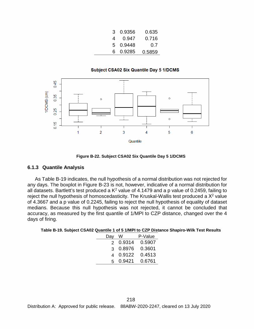
218 Distribution A: Approved for public release. 88ABW-2020-2247, cleared on 13 July 2020
3 0.9356 0.635 4 0.947 0.716 5 0.9448 0.7 6 0.9285 0.5859
Figure B-22. Subject CSA02 Six Quantile Day 5 1/DCMS
6.1.3 Quantile Analysis
As Table B-19 indicates, the null hypothesis of a normal distribution was not rejected for any days. The boxplot in Figure B-23 is not, however, indicative of a normal distribution for all datasets. Bartlett’s test produced a K2 value of 4.1479 and a p value of 0.2459, failing to reject the null hypothesis of homoscedasticity. The Kruskal-Wallis test produced a Χ2 value of 4.3667 and a p value of 0.2245, failing to reject the null hypothesis of equality of dataset medians. Because this null hypothesis was not rejected, it cannot be concluded that accuracy, as measured by the first quantile of 1/MPI to CZP distance, changed over the 4 days of firing.
Table B-19. Subject CSA02 Quantile 1 of 5 1/MPI to CZP Distance Shapiro-Wilk Test Results Day W P-Value
2 0.9314 0.5907 3 0.8976 0.3601 4 0.9122 0.4513 5 0.9421 0.6761

219 Distribution A: Approved for public release. 88ABW-2020-2247, cleared on 13 July 2020
Figure B-23. Subject CSA02 Quantile 1 of 5 1/MPI to CZP Distance
As Table B-20 indicates, the null hypothesis of a normal distribution was rejected for day 3. The boxplot in Figure B-24 is not, however, indicative of a normal distribution. Bartlett’s test produced a K2 value of 6.6059 and a p value of 0.08558, failing to reject the null hypothesis of homoscedasticity. The Kruskal-Wallis test produced a Χ2 value of 3.98 and a p value of 0.2636, failing to reject the null hypothesis of equality of dataset medians. Because this null hypothesis was not rejected, it cannot be concluded that accuracy, as measured by the second quantile of 1/MPI to CZP distance, changed over the 4 days of firing.
Table B-20. Subject CSA02 Quantile 2 of 5 1/MPI to CZP Distance Shapiro-Wilk Test Results Day W P-Value
2 0.9164 0.4801 3 0.7456 0.0181 4 0.9166 0.4811 5 0.9797 0.9499

220 Distribution A: Approved for public release. 88ABW-2020-2247, cleared on 13 July 2020
Figure B-24. Subject CSA02 Quantile 2 of 5 1/MPI to CZP Distance
As Table B-21 indicates, the null hypothesis of a normal distribution was rejected for days 2 and 3. The boxplot in Figure B-25 does not provide information to the contrary. Bartlett’s test produced a K2 value of 16.577 and a p value of 0.00008636, rejecting the null hypothesis of homoscedasticity. The Brunner-Dette-Munk test produced an F value of 1.848698 and a p value of 0.1779037, failing to reject the null hypothesis of equality of distribution functions. Because this null hypothesis was not rejected, it cannot be concluded that accuracy, as measured by the third quantile of 1/MPI to CZP distance, changed over the 4 days of firing.
Table B-21. Subject CSA02 Quantile 3 of 5 1/MPI to CZP Distance Shapiro-Wilk Test Results Day W P-Value
2 0.654 0.002 3 0.6115 0.0006 4 0.9331 0.6042 5 0.8994 0.3706

221 Distribution A: Approved for public release. 88ABW-2020-2247, cleared on 13 July 2020
Figure B-25. Subject CSA02 Quantile 3 of 5 1/MPI to CZP Distance
As Table B-22 indicates, the null hypothesis of a normal distribution was rejected for days 3 and 4. The boxplot in Figure B-26 does not provide information to the contrary. Bartlett’s test produced a K2 value of 5.9107 and a p value of 0.116, failing to reject the null hypothesis of homoscedasticity. The Kruskal-Wallis test produced a Χ2 value of 1.2467 and a p value of 0.7418, failing to reject the null hypothesis of equality of dataset medians. Because this null hypothesis was not rejected, it cannot be concluded that accuracy, as measured by the fourth quantile of 1/MPI to CZP distance, changed over the 4 days of firing.
Table B-22. Subject CSA02 Quantile 4/5 1/MPI to CZP Distance Shapiro-Wilk Test Results Day W P-Value
2 0.8258 0.0989 3 0.685 0.0043 4 0.6493 0.0017 5 0.8928 0.3332

222 Distribution A: Approved for public release. 88ABW-2020-2247, cleared on 13 July 2020
Figure B-26. Subject CSA02 Quantile 4 of 5 1/MPI to CZP Distance
As Table B-23 indicates, the null hypothesis of a normal distribution was rejected for day 2. The boxplot in Figure B-27 does not provide information to the contrary. Bartlett’s test produced a K2 value of 6.4342 and a p value of 0.09229, failing to reject the null hypothesis of homoscedasticity. The Kruskal-Wallis test produced a Χ2 value of 1.1467 and a p value of 0.7658, failing to reject the null hypothesis of equality of dataset medians. Because this null hypothesis was not rejected, it cannot be concluded that accuracy, as measured by the fifth quantile of 1/MPI to CZP distance, changed over the 4 days of firing.
Table B-23. Subject CSA02 Quantile 5 of 5 1/MPI to CZP Distance Shapiro-Wilk Test Results Day W P-Value
2 0.6853 0.0043 3 0.8648 0.2063 4 0.9428 0.6815 5 0.889 0.3128

223 Distribution A: Approved for public release. 88ABW-2020-2247, cleared on 13 July 2020
Figure B-27. Subject CSA02 Quantile 5 of 5 1/MPI to CZP Distance
As Table B-24 indicates, the null hypothesis of a normal distribution was rejected for day 3. The boxplot in Figure B-28 does not provide information to the contrary. Bartlett’s test produced a K2 value of 1.5831 and a p value of 0.6632, failing to reject the null hypothesis of homoscedasticity. The Kruskal-Wallis test produced a Χ2 value of 0.18048 and a p value of 0.9807, failing to reject the null hypothesis of equality of dataset medians. Because this null hypothesis was not rejected, it cannot be concluded that accuracy, as measured by the first quantile of 1/DCMS changed over the 4 days of firing.
Table B-24. Subject CSA02 Quantile 1 of 5 1/DCMS Shapiro-Wilk Test Results Day W P-Value
2 0.90384 0.3971 3 0.77828 0.03714 4 0.91433 0.46549 5 0.99061 0.99061

224 Distribution A: Approved for public release. 88ABW-2020-2247, cleared on 13 July 2020
Figure B-28. Subject CSA02 Quantile 1 of 5 1/DCMS
As Table B-25 indicates, the null hypothesis of a normal distribution was rejected for day 3. The boxplot in Figure B-29 does not provide information to the contrary. Bartlett’s test produced a K2 value of 9.1971 and a p value of 0.02678, rejecting the null hypothesis of homoscedasticity. The Brunner-Dette-Munk test produced an F value of 0.9416694 and a p value of 0.4371605, failing to reject the null hypothesis of equality of distribution functions. Because this null hypothesis was not rejected, it cannot be concluded that accuracy, as measured by the second quantile of 1/DCMS changed over the 4 days of firing.
Table B-25. Subject CSA02 Quantile 2 of 5 1/DCMS Shapiro-Wilk Test Results Day W P-Value
2 0.9557 0.7859 3 0.7591 0.0244 4 0.9814 0.9581 5 0.9314 0.5912

225 Distribution A: Approved for public release. 88ABW-2020-2247, cleared on 13 July 2020
Figure B-29. Subject CSA02 Quantile 2 of 5 1/DCMS
As Table B-26 indicates, the null hypothesis of a normal distribution was rejected for day 3. The boxplot in Figure B-30 does not provide information to the contrary. Bartlett’s test produced a K2 value of 4.8488 and a p value of 0.1832, failing to reject the null hypothesis of homoscedasticity. The Kruskal-Wallis test produced a Χ2 value of 1.8467 and a p value of 0.6048, failing to reject the null hypothesis of equality of dataset medians. Because this null hypothesis was not rejected, it cannot be concluded that accuracy, as measured by the third quantile of 1/DCMS changed over the 4 days of firing.
Table B-26. Subject CSA02 Quantile 3 of 5 1/DCMS Shapiro-Wilk Test Results Day W P-Value
2 0.8891 0.3136 3 0.7246 0.0111 4 0.8996 0.3716 5 0.9191 0.4986

226 Distribution A: Approved for public release. 88ABW-2020-2247, cleared on 13 July 2020
Figure B-30. Subject CSA02 Quantile 3 of 5 1/DCMS
As Table B-27 indicates, the null hypothesis of a normal distribution was not rejected for any days. The boxplot in Figure B-31 is not, however, indicative of a normal distribution. Bartlett’s test produced a K2 value of 6.241 and a p value of 0.1005, failing to reject the null hypothesis of homoscedasticity. The Kruskal-Wallis test produced a Χ2 value of 1.8333 and a p value of 0.6077, failing to reject the null hypothesis of equality of dataset medians. Because this null hypothesis was not rejected, it cannot be concluded that accuracy, as measured by the fourth quantile of 1/DCMS changed over the 4 days of firing.
Table B-27. Subject CSA02 Quantile 4 of 5 1/DCMS Shapiro-Wilk Test Results Day W P-Value
2 0.8815 0.2758 3 0.9242 0.536 4 0.8043 0.0643 5 0.8933 0.3357

227 Distribution A: Approved for public release. 88ABW-2020-2247, cleared on 13 July 2020
Figure B-31. Subject CSA02 Quantile 4 of 5 1/DCMS
As Table B-28 indicates, the null hypothesis of a normal distribution was rejected for days 2 and 3. The boxplot in Figure B-32 does not provide information to the contrary. Bartlett’s test produced a K2 value of 1.4299 and a p value of 0.6985, failing to reject the null hypothesis of homoscedasticity. The Kruskal-Wallis test produced a Χ2 value of 6.6933 and a p value of 0.08234, failing to reject the null hypothesis of equality of dataset medians. Because this null hypothesis was not rejected, it cannot be concluded that accuracy, as measured by the fifth quantile of 1/DCMS changed over the 4 days of firing.
Table B-28. Subject CSA02 Quantile 5 of 5 1/DCMS Shapiro-Wilk Test Results Day W P-Value
2 0.7784 0.0373 3 0.801 0.06 4 0.9922 0.9939 5 0.8681 0.2189

228 Distribution A: Approved for public release. 88ABW-2020-2247, cleared on 13 July 2020
Figure B-32. Subject CSA02 Quantile 5 of 5 1/DCMS
As Table B-29 indicates, the null hypothesis of a normal distribution was not rejected for any days. The boxplot in Figure B-33 is not, however, indicative of a normal distribution. Bartlett’s test produced a K2 value of 3.507 and a p value of 0.3199, failing to reject the null hypothesis of homoscedasticity. The Kruskal-Wallis test produced a Χ2 value of 3.7314 and a p value of 0.292, failing to reject the null hypothesis of equality of dataset medians. Because this null hypothesis was not rejected, it cannot be concluded that accuracy, as measured by the first quantile of 1/MPI to CZP distance changed over the 4 days of firing.
Table B-29. Subject CSA02 Quantile 1 of 6 1/MPI to CZP Distance Shapiro-Wilk Test Results Day W P-Value
2 0.8957 0.3867 3 0.9709 0.8807 4 0.97499 0.90622 5 0.9481 0.7236

229 Distribution A: Approved for public release. 88ABW-2020-2247, cleared on 13 July 2020
Figure B-33. Subject CSA02 Quantile 1 of 6 1/MPI to CZP Distance
As Table B-30 indicates, the null hypothesis of a normal distribution was not rejected for any days. The boxplot in Figure B-34 is not, however, indicative of a normal distribution. Bartlett’s test produced a K2 value of 8.0655 and a p value of 0.04468, rejecting the null hypothesis of homoscedasticity. The Brunner-Dette-Munk test produced an F value of 1.303393 and a p value of 0.3107099, failing to reject the null hypothesis of equality of distribution functions. Because this null hypothesis was not rejected, it cannot be concluded that accuracy, as measured by the second quantile of 1/MPI to CZP distance changed over the 4 days of firing.
Table B-30. Subject CSA02 Quantile 2 of 6 1/MPI to CZP Distance Shapiro-Wilk Test Results Day W P-Value
2 0.8849 0.3322 3 0.922 0.543 4 0.96698 0.85552 5 0.9733 0.8962

230 Distribution A: Approved for public release. 88ABW-2020-2247, cleared on 13 July 2020
Figure B-34. Subject CSA02 Quantile 2 of 6 1/MPI to CZP Distance
As Table B-31 indicates, the null hypothesis of a normal distribution was not rejected for any days. The boxplot in Figure B-35 is not, however, indicative of a normal distribution. Bartlett’s test produced a K2 value of 0.38342 and a p value of 0.9436, failing to reject the null hypothesis of homoscedasticity. The Kruskal-Wallis test produced a Χ2 value of 4.7371 and a p value of 0.1921, failing to reject the null hypothesis of equality of dataset medians. Because this null hypothesis was not rejected, it cannot be concluded that accuracy, as measured by the third quantile of 1/MPI to CZP distance changed over the 4 days of firing.
Table B-31. Subject CSA02 Quantile 3 of 6 1/MPI to CZP Distance Shapiro-Wilk Test Results Day W P-Value
2 0.905 0.43814 3 0.80273 0.08527 4 0.89794 0.39859 5 0.95479 0.77129

231 Distribution A: Approved for public release. 88ABW-2020-2247, cleared on 13 July 2020
Figure B-35. Subject CSA02 Quantile 3 of 6 1/MPI to CZP Distance
As Table B-32 indicates, the null hypothesis of a normal distribution was rejected for day 3. The boxplot in Figure B-36 does not provide information to the contrary. Bartlett’s test produced a K2 value of 15.393 and a p value of 0.00151, rejecting the null hypothesis of homoscedasticity. The Brunner-Dette-Munk test produced an F value of 1.771368 and a p value of 0.1985625, failing to reject the null hypothesis of equality of distribution functions. Because this null hypothesis was not rejected, it cannot be concluded that accuracy, as measured by the fourth quantile of 1/MPI to CZP distance changed over the 4 days of firing.
Table B-32. Subject CSA02 Quantile 4 of 6 1/MPI to CZP Distance Shapiro-Wilk Test Results Day W P-Value
2 0.7803 0.0555 3 0.6596 0.0035 4 0.91024 0.46904 5 0.9532 0.7603
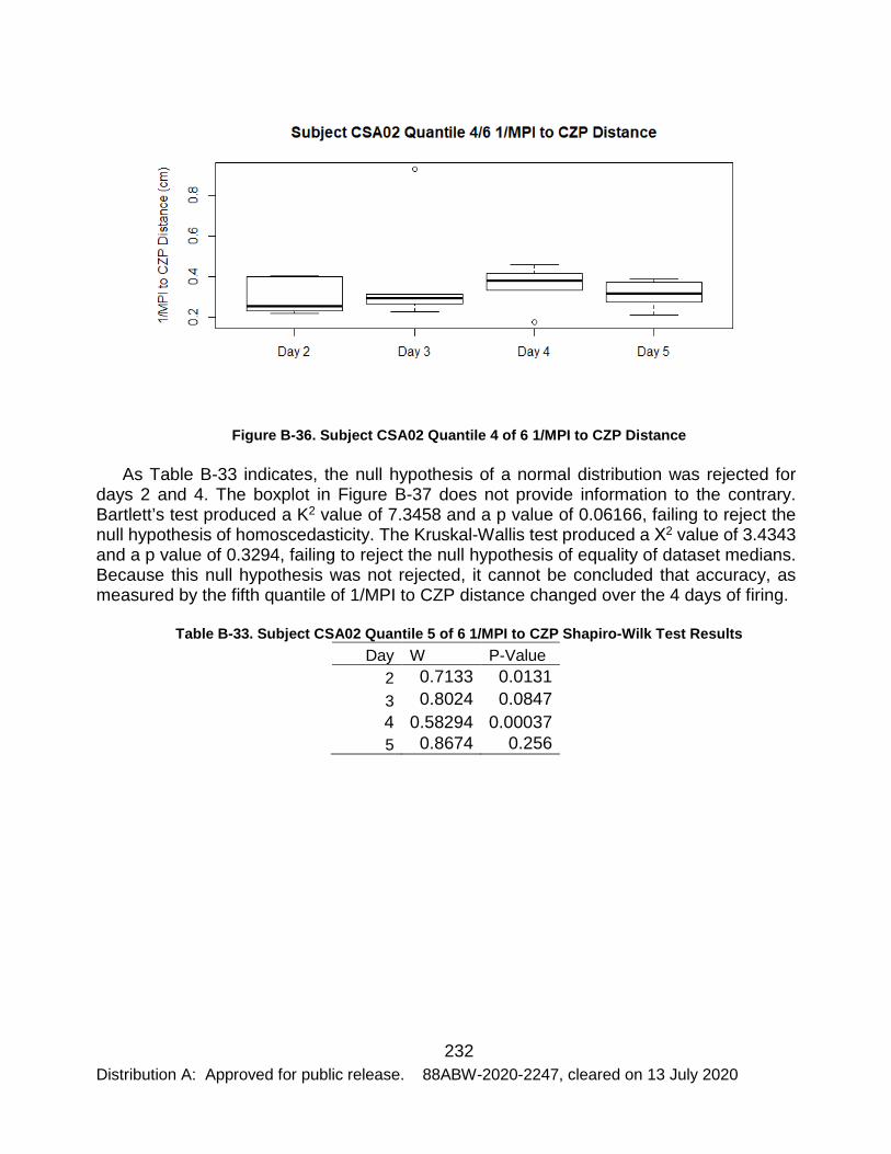
232 Distribution A: Approved for public release. 88ABW-2020-2247, cleared on 13 July 2020
Figure B-36. Subject CSA02 Quantile 4 of 6 1/MPI to CZP Distance
As Table B-33 indicates, the null hypothesis of a normal distribution was rejected for days 2 and 4. The boxplot in Figure B-37 does not provide information to the contrary. Bartlett’s test produced a K2 value of 7.3458 and a p value of 0.06166, failing to reject the null hypothesis of homoscedasticity. The Kruskal-Wallis test produced a Χ2 value of 3.4343 and a p value of 0.3294, failing to reject the null hypothesis of equality of dataset medians. Because this null hypothesis was not rejected, it cannot be concluded that accuracy, as measured by the fifth quantile of 1/MPI to CZP distance changed over the 4 days of firing.
Table B-33. Subject CSA02 Quantile 5 of 6 1/MPI to CZP Shapiro-Wilk Test Results Day W P-Value
2 0.7133 0.0131 3 0.8024 0.0847 4 0.58294 0.00037 5 0.8674 0.256

233 Distribution A: Approved for public release. 88ABW-2020-2247, cleared on 13 July 2020
Figure B-37. Subject CSA02 Quantile 5 of 6 1/MPI to CZP Distance
As Table B-34 indicates, the null hypothesis of a normal distribution was rejected for day 2. The boxplot in Figure B-38 does not provide information to the contrary. Bartlett’s test produced a K2 value of 4.8164 and a p value of 0.1857, failing to reject the null hypothesis of homoscedasticity. The Kruskal-Wallis test produced a Χ2 value of 0.34857 and a p value of 0.9506, failing to reject the null hypothesis of equality of dataset medians. Because this null hypothesis was not rejected, it cannot be concluded that accuracy, as measured by the sixth quantile of 1/MPI to CZP distance changed over the 4 days of firing.
Table B-34. Subject CSA02 Quantile 6 of 6 1/MPI to CZP Distance Shapiro-Wilk Test Results Day W P-Value
2 0.7374 0.0226 3 0.825 0.1276 4 0.9659 0.8481 5 0.9328 0.6159

234 Distribution A: Approved for public release. 88ABW-2020-2247, cleared on 13 July 2020
Figure B-38. Subject CSA02 Quantile 6 of 6 1/MPI to CZP Distance
As Table B-35 indicates, the null hypothesis of a normal distribution was not rejected for any days. The boxplot in Figure B-39 does not provide information to the contrary. Bartlett’s test produced a K2 value of 3.9437 and a p value of 0.2676, failing to reject the null hypothesis of homoscedasticity. The Kruskal-Wallis test produced a Χ2 value of 1.1486 and a p value of 0.7654, failing to reject the null hypothesis of equality of dataset medians. Because this null hypothesis was not rejected, it cannot be concluded that accuracy, as measured by the first quantile of 1/DCMS changed over the 4 days of firing.
Table B-35. Subject CSA02 Quantile 1 of 6 1/DCMS Shapiro-Wilk Test Results Day W P-Value
2 0.90747 0.4525 3 0.89067 0.3605 4 0.93225 0.6118 5 0.9884 0.9737

235 Distribution A: Approved for public release. 88ABW-2020-2247, cleared on 13 July 2020
Figure B-39. Subject CSA02 Quantile 1 of 6 1/DCMS
As Table B-36 indicates, the null hypothesis of a normal distribution was not rejected for any days. The boxplot in Figure B-40 is not, however, indicative of a normal distribution. Bartlett’s test produced a K2 value of 7.2976 and a p value of 0.06299, failing to reject the null hypothesis of homoscedasticity. The Kruskal-Wallis test produced a Χ2 value of 1.4686 and a p value of 0.6895, failing to reject the null hypothesis of equality of dataset medians. Because this null hypothesis was not rejected, it cannot be concluded that accuracy, as measured by the second quantile of 1/DCMS changed over the 4 days of firing.
Table B-36. Subject CSA02 Quantile 2 of 6 1/DCMS Shapiro-Wilk Test Results Day W P-Value
2 0.95201 0.7516 3 0.85956 0.2267 4 0.9794 0.9314 5 0.86007 0.2285

236 Distribution A: Approved for public release. 88ABW-2020-2247, cleared on 13 July 2020
Figure B-40. Subject CSA02 Quantile 2 of 6 1/DCMS
As Table B-37 indicates, the null hypothesis of a normal distribution was not rejected for any days. The boxplot in Figure B-41 is not, however, indicative of a normal distribution. Bartlett’s test produced a K2 value of 4.0939 and a p value of 0.2515, failing to reject the null hypothesis of homoscedasticity. The Kruskal-Wallis test produced a Χ2 value of 4.0514 and a p value of 0.256, failing to reject the null hypothesis of equality of dataset medians. Because this null hypothesis was not rejected, it cannot be concluded that accuracy, as measured by the third quantile of 1/DCMS changed over the 4 days of firing.
Table B-37. Subject CSA02 Quantile 3 of 6 1/DCMS Shapiro-Wilk Test Results Day W P-Value
2 0.96978 0.8738 3 0.83473 0.1509 4 0.93556 0.6347 5 0.9356 0.635

237 Distribution A: Approved for public release. 88ABW-2020-2247, cleared on 13 July 2020
Figure B-41. Subject CSA02 Quantile 3 of 6 1/DCMS
As Table B-38 indicates, the null hypothesis of a normal distribution was rejected for day 3. The boxplot in Figure B-42 does not provide information to the contrary. Bartlett’s test produced a K2 value of 1.9382 and a p value of 0.5853, failing to reject the null hypothesis of homoscedasticity. The Kruskal-Wallis test produced a Χ2 value of 0.12 and a p value of 0.9893, failing to reject the null hypothesis of equality of dataset medians. Because this null hypothesis was not rejected, it cannot be concluded that accuracy, as measured by the fourth quantile of 1/DCMS changed over the 4 days of firing.
Table B-38. Subject CSA02 Quantile 4 of 6 1/DCMS Shapiro-Wilk Test Results Day W P-Value
2 0.79468 0.07328 3 0.70179 0.009997 4 0.90294 0.4264 5 0.94704 0.716

238 Distribution A: Approved for public release. 88ABW-2020-2247, cleared on 13 July 2020
Figure B-42. Subject CSA02 Quantile 4 of 6 1/DCMS
As Table B-39 indicates, the null hypothesis of a normal distribution was not rejected for any days. The boxplot in Figure B-43 does not, however, support a normal distribution. Bartlett’s test produced a K2 value of 3.7612 and a p value of 0.2884, failing to reject the null hypothesis of homoscedasticity. The Kruskal-Wallis test produced a Χ2 value of 0.062857 and a p value of 0.9959, failing to reject the null hypothesis of equality of dataset medians. Because this null hypothesis was not rejected, it cannot be concluded that accuracy, as measured by the fifth quantile of 1/DCMS changed over the 4 days of firing.
Table B-39. Subject CSA02 Quantile 5 of 6 1/DCMS Shapiro-Wilk Test Results Day W P-Value
2 0.87435 0.2845 3 0.88843 0.3493 4 0.88211 0.319 5 0.94479 0.7
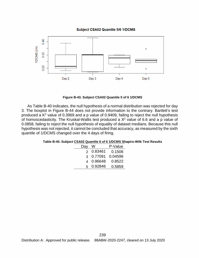
239 Distribution A: Approved for public release. 88ABW-2020-2247, cleared on 13 July 2020
Figure B-43. Subject CSA02 Quantile 5 of 6 1/DCMS
As Table B-40 indicates, the null hypothesis of a normal distribution was rejected for day 3. The boxplot in Figure B-44 does not provide information to the contrary. Bartlett’s test produced a K2 value of 0.3969 and a p value of 0.9409, failing to reject the null hypothesis of homoscedasticity. The Kruskal-Wallis test produced a Χ2 value of 6.6 and a p value of 0.0858, failing to reject the null hypothesis of equality of dataset medians. Because this null hypothesis was not rejected, it cannot be concluded that accuracy, as measured by the sixth quantile of 1/DCMS changed over the 4 days of firing.
Table B-40. Subject CSA02 Quantile 6 of 6 1/DCMS Shapiro-Wilk Test Results Day W P-Value
2 0.83461 0.1506 3 0.77091 0.04596 4 0.96648 0.8522 5 0.92846 0.5859

240 Distribution A: Approved for public release. 88ABW-2020-2247, cleared on 13 July 2020
Figure B-44. Subject CSA02 Quantile 5 of 6 1/DCMS
6.1.4 Correlation Results
In Table B-41, the results of the Pearson, Kendall, and Spearman tests for correlation between shot timing and the distance from the shot to the center of the target are shown. As Table B-41 indicates, the respective null hypotheses of no correlation for all tests were rejected on days 3 and 4. While the correlations were significant, they were weak as shown by the fact that the largest coefficient was 0.234724.
Table B-41. Subject CSA02 Correlation Results Pearson Kendall Spearman
Day T P-Value Coefficient Z P-Value Tau S P-Value Rho 2 -0.54397 0.5878 -0.05789 -0.17777 0.8589 -0.01277 124210 0.8338 -0.02242 3 2.2652 0.02596 0.234724 1.9798 0.04772 0.142125 96123 0.0483 0.208771 4 2.1935 0.03091 0.227686 2.0846 0.03711 0.149819 94077 0.03251 0.225612 5 -1.1714 0.2446 -0.1239 -1.1468 0.2515 -0.08239 137750 0.2084 -0.13386
6.2 Subject CSA03 Results 6.2.1 IES Scoring Results
As Figure B-45 indicates, MPI to CZP distanced based IES scores were relatively consistent across all days of firing for radii of 5 and 4 cm. A radius of 3 cm showed an increase from day 2 to day 4, after which it decreased to a level close to that of day 2. At a radius of 2 cm, there was a slight decrease from day 2 to day 3, after which there was a significant increase through day 5.
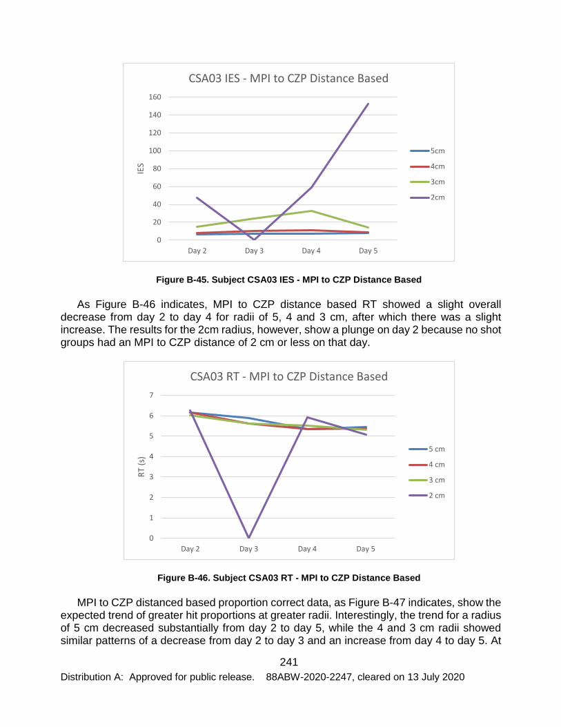
241 Distribution A: Approved for public release. 88ABW-2020-2247, cleared on 13 July 2020
Figure B-45. Subject CSA03 IES - MPI to CZP Distance Based
As Figure B-46 indicates, MPI to CZP distance based RT showed a slight overall decrease from day 2 to day 4 for radii of 5, 4 and 3 cm, after which there was a slight increase. The results for the 2cm radius, however, show a plunge on day 2 because no shot groups had an MPI to CZP distance of 2 cm or less on that day.
Figure B-46. Subject CSA03 RT - MPI to CZP Distance Based
MPI to CZP distanced based proportion correct data, as Figure B-47 indicates, show the expected trend of greater hit proportions at greater radii. Interestingly, the trend for a radius of 5 cm decreased substantially from day 2 to day 5, while the 4 and 3 cm radii showed similar patterns of a decrease from day 2 to day 3 and an increase from day 4 to day 5. At
0
20
40
60
80
100
120
140
160
Day 2 Day 3 Day 4 Day 5
IES
CSA03 IES - MPI to CZP Distance Based
5cm
4cm
3cm
2cm
0
1
2
3
4
5
6
7
Day 2 Day 3 Day 4 Day 5
RT (s
)
CSA03 RT - MPI to CZP Distance Based
5 cm
4 cm
3 cm
2 cm

242 Distribution A: Approved for public release. 88ABW-2020-2247, cleared on 13 July 2020
a radius of 2 cm, however, the trend was different with a decrease followed by an increase followed by a decrease.
Figure B-47. Subject CSA03 Proportion Correct - MPI to CZP Distance Based
As Figure B-48 shows, DCMS based IES trends were very similar for radii of 5 and 4 cm, but differed significantly for 3 and 2 cm. At a radius of 3 cm, IES increased from day 2 to day 4, after which it decreased significantly. At a radius of 2 cm, IES increased significantly from day 2 to day 3, after which it decreased through day 5.
Figure B-48. Subject CSA03 IES – DCMS Based
As Figure B-49 shows, DCMS based RT for radii of 5, 4 and 3 cm showed an overall
00.10.20.30.40.50.60.70.80.9
1
Day 2 Day 3 Day 4 Day 5
Prop
ortio
n Co
rrec
t
CSA03 Proportion Correct - MPI to CZP Distance Based
5 cm
4 cm
3 cm
2 cm
0
20
40
60
80
100
120
Day 2 Day 3 Day 4 Day 5
IES
CSA03 IES - DCMS Based
5cm
4cm
3cm
2cm

243 Distribution A: Approved for public release. 88ABW-2020-2247, cleared on 13 July 2020
decreasing trend, while the 2cm data showed a similar trend punctuated by a more dramatic decrease from day 2 to day 3.
Figure B-49. Subject CSA03 RT - DCMS Based
Figure B-50 shows the expected trend of greater hit proportions with greater DCMS based radius. At a radius of 5 cm, there was an overall decrease in proportion, while at radii of 4, 3 and 2 cm there was a decrease followed by an increase.
Figure B-50. Subject CSA03 Proportion Correct - DCMS Based
0
1
2
3
4
5
6
7
Day 2 Day 3 Day 4 Day 5
RT (s
)
CSA03 RT - DCMS Based
5 cm
4 cm
3 cm
2 cm
0
0.1
0.2
0.3
0.4
0.5
0.6
0.7
0.8
0.9
1
Day 2 Day 3 Day 4 Day 5
Prop
ortio
n Co
rrec
t
CSA03 Proportion Correct DCMS - Based
5 cm
4 cm
3 cm
2 cm

244 Distribution A: Approved for public release. 88ABW-2020-2247, cleared on 13 July 2020
6.2.2 Conditional Accuracy Function Results
As Table B-42 indicates, the null hypothesis of a normal distribution was rejected for quantile 5. The boxplot in Figure B-51 does not provide information to the contrary. Bartlett’s test produced a K2 value of 11.659 and a p value of 0.02008, rejecting the null hypothesis of homoscedasticity. The Brunner-Dette-Munk test produced an F value of 0.7113653 and a p value of 0.577957, failing to reject the null hypothesis of equality of distribution functions. Because this null hypothesis was not rejected, it cannot be concluded that accuracy, as measured by 1/MPI to CZP distance, differed by time quantile on day 2.
Table B-42. Subject CSA03 Five Quantile Day 2 1/MPI to CZP Distance Shapiro-Wilk Test Results Quantile W P-Value
1 0.8671 0.2148 2 0.897 0.3567 3 0.8717 0.2331 4 0.8672 0.2154 5 0.6632 0.0025
Figure B-51. Subject CSA03 Five Quantile Day 2 1/MPI to CZP Distance
As Table B-43 indicates, the null hypothesis of a normal distribution was rejected for quantile 5. The boxplot in Figure B-52 does not provide information to the contrary. Bartlett’s test produced a K2 value of 12.494 and a p value of 0.01403, rejecting the null hypothesis of homoscedasticity. The Brunner-Dette-Munk test produced an F value of 0.6815939 and a p value of 0.5968041, failing to reject the null hypothesis of equality of distribution functions. Because this null hypothesis was not rejected, it cannot be concluded that accuracy, as measured by 1/DCMS, differed by time quantile on day 2.
Table B-43. Subject CSA03 Five Quantile Day 2 1/DCMS Shapiro-Wilk Test Results

245 Distribution A: Approved for public release. 88ABW-2020-2247, cleared on 13 July 2020
Quantile W P-Value 1 0.9351 0.6197 2 0.9111 0.4438 3 0.8565 0.1776 4 0.9721 0.9063 5 0.762 0.026
Figure B-52. Subject CSA03 Five Quantile Day 2 1/DCMS
As Table B-44 indicates, the null hypothesis of a normal distribution was rejected for quantile 2. The boxplot in Figure B-53 does not provide information to the contrary. Bartlett’s test produced a K2 value of 2.2259 and a p value of 0.6943, failing to reject the null hypothesis of homoscedasticity. The Kruskal-Wallis test produced a Χ2 value of 3.6602 and a p value of 0.4539, failing to reject the null hypothesis of equality of dataset medians. Because this null hypothesis was not rejected, it cannot be concluded that accuracy, as measured by 1/MPI to CZP distance, differed by time quantile on day 3.
Table B-44. Subject CSA03 Five Quantile Day 3 1/MPI to CZP Distance Shapiro-Wilk Test Results Quantile W P-Value
1 0.8594 0.187 2 0.7847 0.0426 3 0.9253 0.5445 4 0.848 0.1516

246 Distribution A: Approved for public release. 88ABW-2020-2247, cleared on 13 July 2020
5 0.9441 0.6922
Figure B-53. Subject CSA03 Five Quantile Day 3 1/MPI to CZP Distance
As Table B-45 indicates, the null hypothesis of a normal distribution was rejected for quantiles 2 and 3. The boxplot in Figure B-54 does not provide information to the contrary. Bartlett’s test produced a K2 value of 5.3662 and a p value of 0.2517, failing reject the null hypothesis of homoscedasticity. The Kruskal-Wallis test produced a Χ2 value of 3.4882 and a p value of 0.4797, failing to reject the null hypothesis of equality of dataset medians. Because this null hypothesis was not rejected, it cannot be concluded that accuracy, as measured by 1/DCMS, differed by time quantile on day 3.
Table B-45. Subject CSA03 Five Quantile Day 3 1/DCMS Shapiro-Wilk Test Results Quantile W P-Value
1 0.8917 0.3271 2 0.7068 0.0073 3 0.7837 0.0417 4 0.9242 0.536 5 0.801 0.06

247 Distribution A: Approved for public release. 88ABW-2020-2247, cleared on 13 July 2020
Figure B-54. Subject CSA03 Five Quantile Day 3 1/DCMS
As Table B-46 indicates, the null hypothesis of a normal distribution was rejected for quantile 5. The boxplot in Figure B-55 does not provide information to the contrary. Bartlett’s test produced a K2 value of 10.304 and a p value of 0.03561, rejecting the null hypothesis of homoscedasticity. The Brunner-Dette-Munk test produced an F value of 0.8330532 and a p value of 0.5124386, failing to reject the null hypothesis of equality of distribution functions. Because this null hypothesis was not rejected, it cannot be concluded that accuracy, as measured by 1/MPI to CZP distance, differed by time quantile on day 4.
Table B-46. Subject CSA03 Five Quantile Day 4 1/MPI to CZP Distance Shapiro-Wilk Test Results Quantile W P-Value
1 0.9835 0.9676 2 0.8836 0.286 3 0.8001 0.0588 4 0.8783 0.2612 5 0.6162 0.0007

248 Distribution A: Approved for public release. 88ABW-2020-2247, cleared on 13 July 2020
Figure B-55. Subject CSA03 Five Quantile Day 4 1/MPI to CZP Distance
As Table B-47 indicates, the null hypothesis of a normal distribution was rejected for quantile 1. The boxplot in Figure B-56 does not provide information to the contrary. Bartlett’s test produced a K2 value of 14.334 and a p value of 0.006302, rejecting the null hypothesis of homoscedasticity. The Brunner-Dette-Munk test produced an F value of 0.7857501 and a p value of 0.5335947, failing to reject the null hypothesis of equality of distribution functions. Because this null hypothesis was not rejected, it cannot be concluded that accuracy, as measured by 1/DCMS, differed by time quantile on day 4.
Table B-47. Subject CSA03 Five Quantile Day 4 1/DCMS Shapiro-Wilk Test Results Quantile W P-Value
1 0.748 0.019 2 0.8766 0.2537 3 0.9425 0.6792 4 0.9374 0.6379 5 0.8614 0.1941

249 Distribution A: Approved for public release. 88ABW-2020-2247, cleared on 13 July 2020
Figure B-56. Subject CSA03 Five Quantile Day 4 1/DCMS
As Table B-48 indicates, the null hypothesis of a normal distribution was not rejected for any quantiles. The boxplot in Figure B-57 is not, however, indicative of a normal distribution. Bartlett’s test produced a K2 value of 15.556 and a p value of 0.008232, rejecting the null hypothesis of homoscedasticity. The Brunner-Dette-Munk test produced an F value of 0.7904519 and a p value of 0.5384977, failing to reject the null hypothesis of equality of distribution functions. Because this null hypothesis was not rejected, it cannot be concluded that accuracy, as measured by 1/MPI to CZP distance, differed by time quantile on day 5.
Table B-48. Subject CSA03 Five Quantile Day 5 1/MPI to CZP Distance Shapiro-Wilk Test Results Quantile W P-Value
1 0.8507 0.1595 2 0.8176 0.0841 3 0.937 0.635 4 0.9382 0.6449 5 0.8949 0.3449

250 Distribution A: Approved for public release. 88ABW-2020-2247, cleared on 13 July 2020
Figure B-57. Subject CSA03 Five Quantile Day 5 1/MPI to CZP Distance
As Table B-49 indicates, the null hypothesis of a normal distribution was rejected for quantile 4. The boxplot in Figure B-58 does not provide information to the contrary. Bartlett’s test produced a K2 value of 5.7509 and a p value of 0.2222, failing to reject the null hypothesis of homoscedasticity. The Kruskal-Wallis test produced a Χ2 value of 3.5871 and a p value of 0.4648, failing to reject the null hypothesis of equality of dataset medians. Because this null hypothesis was not rejected, it cannot be concluded that accuracy, as measured by 1/DCMS, differed by time quantile on day 5.
Table B-49. Subject CSA03 Five Quantile Day 5 1/DCMS Shapiro-Wilk Test Results Quantile W P-Value
1 0.794 0.0518 2 0.8917 0.3272 3 0.8717 0.2331 4 0.787 0.0448 5 0.8292 0.1059

251 Distribution A: Approved for public release. 88ABW-2020-2247, cleared on 13 July 2020
Figure B-58. Subject CSA03 Five Quantile Day 5 1/DCMS
As Table B-50 indicates, the null hypothesis of a normal distribution was rejected for quantile 6. The boxplot in Figure B-59 does not provide information to the contrary. Bartlett’s test produced a K2 value of 16.578 and a p value of 0.005373, rejecting the null hypothesis of homoscedasticity. The Brunner-Dette-Munk test produced an F value of 0.3607348 and a p value of 0.8337162, failing to reject the null hypothesis of equality of distribution functions. Because this null hypothesis was not rejected, it cannot be concluded that accuracy, as measured by 1/MPI to CZP distance, differed by time quantile on day 2.
Table B-50. Subject CSA03 Six Quantile Day 2 1/MPI to CZP Distance Shapiro-Wilk Test Results Quantile W P-Value
1 0.917 0.511 2 0.9051 0.4385 3 0.9022 0.422 4 0.948 0.7228 5 0.9052 0.4393 6 0.6996 0.0095

252 Distribution A: Approved for public release. 88ABW-2020-2247, cleared on 13 July 2020
Figure B-59. Subject CSA03 Six Quantile Day 2 1/MPI to CZP Distance
As Table B-51 indicates, the null hypothesis of a normal distribution was rejected for quantile 6. The boxplot in Figure B-60 does not provide information to the contrary. Bartlett’s test produced a K2 value of 12.291 and a p value of 0.03102, rejecting the null hypothesis of homoscedasticity. The Brunner-Dette-Munk test produced an F value of 1.563851 and a p value of 0.2128644, failing to reject the null hypothesis of equality of distribution functions. Because this null hypothesis was not rejected, it cannot be concluded that accuracy, as measured by 1/DCMS, differed by time quantile on day 2.
Table B-51. Subject CSA03 Six Quantile Day 2 1/DCMS Shapiro-Wilk Test Results Quantile W P-Value
1 0.9571 0.7877 2 0.9773 0.9195 3 0.9834 0.9521 4 0.9144 0.4944 5 0.9589 0.8004 6 0.7155 0.0138

253 Distribution A: Approved for public release. 88ABW-2020-2247, cleared on 13 July 2020
Figure B-60. Subject CSA03 Six Quantile Day 2 1/DCMS
As Table B-52 indicates, the null hypothesis of a normal distribution was rejected for quantile 2. The boxplot in Figure B-61 does not provide information to the contrary. Bartlett’s test produced a K2 value of 6.7722 and a p value of 0.2381, failing to reject the null hypothesis of homoscedasticity. The Kruskal-Wallis test produced a Χ2 value of 9.0258 and a p value of 0.108, failing to reject the null hypothesis of equality of dataset medians. Because this null hypothesis was not rejected, it cannot be concluded that accuracy, as measured by 1/MPI to CZP distance, differed by time quantile on day 3.
Table B-52. Subject CSA03 Six Quantile Day 3 1/MPI to CZP Distance Shapiro-Wilk Test Results Quantile W P-Value
1 0.9013 0.4172 2 0.715 0.0136 3 0.932 0.61 4 0.9755 0.909 5 0.8722 0.2754 6 0.9193 0.5254

254 Distribution A: Approved for public release. 88ABW-2020-2247, cleared on 13 July 2020
Figure B-61. Subject CSA03 Six Quantile Day 3 1/MPI to CZP Distance
As Table B-53 indicates, the null hypothesis of a normal distribution was rejected for quantiles 3, 4 and 6. The boxplot in Figure B-62 does not provide information to the contrary. Bartlett’s test produced a K2 value of 6.0796 and a p value of 0.2985, failing to reject the null hypothesis of homoscedasticity. The Kruskal-Wallis test produced a Χ2 value of 4.3497 and a p value of 0.5002, failing to reject the null hypothesis of equality of dataset medians. Because this null hypothesis was not rejected, it cannot be concluded that accuracy, as measured by 1/DCMS, differed by time quantile on day 3.
Table B-53. Subject CSA03 Six Quantile Day 3 1/DCMS Shapiro-Wilk Test Results Quantile W P-Value
1 0.8111 0.0995 2 0.8031 0.0858 3 0.7635 0.0395 4 0.7552 0.0332 5 0.8884 0.3493 6 0.7708 0.0459

255 Distribution A: Approved for public release. 88ABW-2020-2247, cleared on 13 July 2020
Figure B-62. Subject CSA03 Six Quantile Day 3 1/DCMS
As Table B-54 indicates, the null hypothesis of a normal distribution was rejected for quantile 6. The boxplot in Figure B-63 does not provide information to the contrary. Bartlett’s test produced a K2 value of 15.556 and a p value of 0.008232, rejecting the null hypothesis of homoscedasticity. The Brunner-Dette-Munk test produced an F value of 0.860021 and a p value of 0.5154562, failing to reject the null hypothesis of equality of distribution functions. Because this null hypothesis was not rejected, it cannot be concluded that accuracy, as measured by 1/MPI to CZP distance, differed by time quantile on day 4.
Table B-54. Subject CSA03 Six Quantile Day 4 1/MPI to CZP Distance Shapiro-Wilk Test Results Quantile W P-Value
1 0.964 0.8357 2 0.9066 0.4475 3 0.8752 0.288 4 0.8638 0.2421 5 0.9686 0.8664 6 0.6724 0.0048

256 Distribution A: Approved for public release. 88ABW-2020-2247, cleared on 13 July 2020
Figure B-63. Subject CSA03 Six Quantile Day 4 1/MPI to CZP Distance
As Table B-55 indicates, the null hypothesis of a normal distribution was rejected for quantiles 3, 4 and 6. The boxplot in Figure B-64 does not provide information to the contrary. Bartlett’s test produced a K2 value of 14.837 and a p value of 0.01108, rejecting the null hypothesis of homoscedasticity. The Brunner-Dette-Munk test produced an F value of 0.6573047 and a p value of 0.6346021, failing to reject the null hypothesis of equality of distribution functions. Because this null hypothesis was not rejected, it cannot be concluded that accuracy, as measured by 1/DCMS, differed by time quantile on day 4.
Table B-55. Subject CSA03 Six Quantile Day 4 1/DCMS Shapiro-Wilk Test Results Quantile W P-Value
1 0.8111 0.0995 2 0.8031 0.0858 3 0.7635 0.0395 4 0.7552 0.0332 5 0.8884 0.3493 6 0.7708 0.0459

257 Distribution A: Approved for public release. 88ABW-2020-2247, cleared on 13 July 2020
Figure B-64. Subject CSA03 Six Quantile Day 4 1/DCMS
As Table B-56 indicates, the null hypothesis of a normal distribution was not rejected for any quantiles. The boxplot in Figure B-65 is not, however, indicative of a normal distribution. Bartlett’s test produced a K2 value of 0.58913 and a p value of 0.9885, failing to reject the null hypothesis of homoscedasticity. The Kruskal-Wallis test produced a Χ2 value of 2.8684 and a p value of 0.7203, failing to reject the null hypothesis of equality of dataset medians. Because this null hypothesis was not rejected, it cannot be concluded that accuracy, as measured by 1/MPI to CZP distance, differed by time quantile on day 5.
Table B-56. Subject CSA03 Six Quantile Day 5 1/MPI to CZP Distance Shapiro-Wilk Test Results Quantile W P-Value
1 0.8894 0.3542 2 0.8261 0.1299 3 0.8272 0.1326 4 0.8883 0.3489 5 0.9936 0.9906 6 0.9287 0.5872

258 Distribution A: Approved for public release. 88ABW-2020-2247, cleared on 13 July 2020
Figure B-65. Subject CSA03 Six Quantile Day 5 1/MPI to CZP Distance
As Table B-57 indicates, the null hypothesis of a normal distribution was not rejected for any quantiles. The boxplot in Figure B-66 is not, however, indicative of a normal distribution. Bartlett’s test produced a K2 value of 16.741 and a p value of 0.005017, rejecting the null hypothesis of homoscedasticity. The Brunner-Dette-Munk test produced an F value of 1.698795 and a p value of 0.198044, failing to reject the null hypothesis of equality of distribution functions. Because this null hypothesis was not rejected, it cannot be concluded that accuracy, as measured by 1/DCMS, differed by time quantile on day 5.
Table B-57. Subject CSA03 Six Quantile Day 5 1/DCMS Shapiro-Wilk Test Results Quantile W P-Value
1 0.8086 0.095 2 0.9482 0.7246 3 0.9074 0.4519 4 0.9827 0.9486 5 0.9146 0.4958 6 0.8771 0.2964

259 Distribution A: Approved for public release. 88ABW-2020-2247, cleared on 13 July 2020
Figure B-66. Subject CSA034 Six Quantile Day 5 1/DCMS
6.2.3 Quantile Analysis
As Table B-58 indicates, the null hypothesis of a normal distribution was not rejected for any days. The boxplot in Figure B-67 is not, however, indicative of a normal distribution. Bartlett’s test produced a K2 value of 0.60462 and a p value of 0.8954, failing to reject the null hypothesis of homoscedasticity. The Kruskal-Wallis test produced a Χ2 value of 0.42 and a p value of 0.9361, failing to reject the null hypothesis of equality of dataset medians. Because this null hypothesis was not rejected, it cannot be concluded that accuracy, as measured by the first quantile of 1/MPI to CZP distance changed over the 4 days of firing.
Table B-58. Subject CSA03 Quantile 1 of 5 1/MPI to CZP Distance Shapiro-Wilk Test Results Day W P-Value
2 0.86709 0.21484 3 0.85938 0.18703 4 0.98349 0.96755 5 0.85071 0.15951

260 Distribution A: Approved for public release. 88ABW-2020-2247, cleared on 13 July 2020
Figure B-67. Subject CSA03 Quantile 1 of 5 1/MPI to CZP Distance
As Table B-59 indicates, the null hypothesis of a normal distribution was rejected for day 3. The boxplot in Figure B-68 does not provide information to the contrary. Bartlett’s test produced a K2 value of 5.3374 and a p value of 0.1487, failing to reject the null hypothesis of homoscedasticity. The Kruskal-Wallis test produced a Χ2 value of 3.98 and a p value of 0.2636, failing to reject the null hypothesis of equality of dataset medians. Because this null hypothesis was not rejected, it cannot be concluded that accuracy, as measured by the second quantile of 1/MPI to CZP distance changed over the 4 days of firing.
Table B-59. Subject CSA03 Quantile 2 of 5 1/MPI to CZP Distance Shapiro-Wilk Test Results Day W P-Value
2 0.89704 0.35675 3 0.78471 0.04263 4 0.88359 0.28595 5 0.81759 0.0841

261 Distribution A: Approved for public release. 88ABW-2020-2247, cleared on 13 July 2020
Figure B-68. Subject CSA03 Quantile 2 of 5 1/MPI to CZP Distance
As Table B-60 indicates, the null hypothesis of a normal distribution was not rejected for any days. The boxplot in Figure B-69 is not, however, indicative of a normal distribution. Bartlett’s test produced a K2 value of 5.143 and a p value of 0.1616, failing to reject the null hypothesis of homoscedasticity. The Kruskal-Wallis test produced a Χ2 value of 1.5933 and a p value of 0.6609, failing to reject the null hypothesis of equality of dataset medians. Because this null hypothesis was not rejected, it cannot be concluded that accuracy, as measured by the third quantile of 1/MPI to CZP distance changed over the 4 days of firing.
Table B-60. Subject CSA03 Quantile 3 of 5 1/MPI to CZP Distance Shapiro-Wilk Test Results Day W P-Value
2 0.87171 0.23313 3 0.92533 0.54454 4 0.80006 0.05885 5 0.93699 0.63503

262 Distribution A: Approved for public release. 88ABW-2020-2247, cleared on 13 July 2020
Figure B-69. Subject CSA03 Quantile 3 of 5 1/MPI to CZP Distance
As Table B-61 indicates, the null hypothesis of a normal distribution was not rejected for any days. The boxplot in Figure B-70 is not, however, indicative of a normal distribution. Bartlett’s test produced a K2 value of 3.8544 and a p value of 0.2776, failing to reject the null hypothesis of homoscedasticity. The Kruskal-Wallis test produced a Χ2 value of 5.66 and a p value of 0.1294, failing to reject the null hypothesis of equality of dataset medians. Because this null hypothesis was not rejected, it cannot be concluded that accuracy, as measured by the fourth quantile of 1/MPI to CZP distance changed over the 4 days of firing.
Table B-61. Subject CSA03 Quantile 4 of 5 1/MPI to CZP Distance Shapiro-Wilk Test Results Day W P-Value
2 0.86723 0.21538 3 0.84799 0.1516 4 0.87827 0.26122 5 0.93822 0.64492

263 Distribution A: Approved for public release. 88ABW-2020-2247, cleared on 13 July 2020
Figure B-70. Subject CSA03 Quantile 4 of 5 1/MPI to CZP Distance
As Table B-62 indicates, the null hypothesis of a normal distribution was rejected for days 2 and 4. The boxplot in Figure B-71 does not provide information to the contrary. Bartlett’s test produced a K2 value of 4.8688 and a p value of 0.1817, failing to reject the null hypothesis of homoscedasticity. The Kruskal-Wallis test produced a Χ2 value of 3.0867 and a p value of 0.3785, failing to reject the null hypothesis of equality of dataset medians. Because this null hypothesis was not rejected, it cannot be concluded that accuracy, as measured by the fifth quantile of 1/MPI to CZP distance changed over the 4 days of firing.
Table B-62. Subject CSA03 Quantile 5 of 5 1/MPI to CZP Distance Shapiro-Wilk Test Results Day W P-Value
2 0.66324 0.00248 3 0.94408 0.69224 4 0.61624 0.00072 5 0.89494 0.34489

264 Distribution A: Approved for public release. 88ABW-2020-2247, cleared on 13 July 2020
Figure B-71. Subject CSA03 Quantile 5 of 5 1/MPI to CZP Distance
As Table B-63 indicates, the null hypothesis of a normal distribution was rejected for day 4. The boxplot in Figure B-72 does not provide information to the contrary. Bartlett’s test produced a K2 value of 5.5446 and a p value of 0.136, failing to reject the null hypothesis of homoscedasticity. The Kruskal-Wallis test produced a Χ2 value of 2.26 and a p value of 0.5202, failing to reject the null hypothesis of equality of dataset medians. Because this null hypothesis was not rejected, it cannot be concluded that accuracy, as measured by the first quantile of 1/DCMS changed over the 4 days of firing.
Table B-63. Subject CSA03 Quantile 1 of 5 1/DCMS Shapiro-Wilk Test Results Day W P-Value
2 0.93506 0.61967 3 0.89168 0.32708 4 0.748 0.01904 5 0.79395 0.05182

265 Distribution A: Approved for public release. 88ABW-2020-2247, cleared on 13 July 2020
Figure B-72. Subject CSA03 Quantile 1/5 1/DCMS
As Table B-64 indicates, the null hypothesis of a normal distribution was rejected for day 3. The boxplot in Figure B-73 does not provide information to the contrary. Bartlett’s test produced a K2 value of 5.299 and a p value of 0.1512, failing to reject the null hypothesis of homoscedasticity. The Kruskal-Wallis test produced a Χ2 value of 3.84 and a p value of 0.2793, failing to reject the null hypothesis of equality of dataset medians. Because this null hypothesis was not rejected, it cannot be concluded that accuracy, as measured by the second quantile of 1/DCMS changed over the 4 days of firing.
Table B-64. Subject CSA03 Quantile 2 of 5 1/DCMS Shapiro-Wilk Test Results Day W P-Value
2 0.91112 0.44378 3 0.70678 0.00728 4 0.87659 0.25375 5 0.8917 0.32717

266 Distribution A: Approved for public release. 88ABW-2020-2247, cleared on 13 July 2020
Figure B-73. Subject CSA03 Quantile 2 of 5 1/DCMS
As Table B-65 indicates, the null hypothesis of a normal distribution was rejected for day 3. The boxplot in Figure B-74 does not provide information to the contrary. Bartlett’s test produced a K2 value of 14.909 and a p value of 0.001897, rejecting the null hypothesis of homoscedasticity. The Brunner-Dette-Munk test produced an F value of 0.9416694 and a p value of 0.4327972, failing to reject the null hypothesis of equality of distribution functions. Because this null hypothesis was not rejected, it cannot be concluded that accuracy, as measured by the third quantile of 1/DCMS changed over the 4 days of firing.
Table B-65. Subject CSA03 Quantile 3 of 5 1/DCMS Shapiro-Wilk Test Results Day W P-Value
2 0.85653 0.17757 3 0.78371 0.04173 4 0.94247 0.67918 5 0.87171 0.2331

267 Distribution A: Approved for public release. 88ABW-2020-2247, cleared on 13 July 2020
Figure B-74. Subject CSA03 Quantile 3 of 5 1/DCMS
As Table B-66 indicates, the null hypothesis of a normal distribution was rejected for day 5. The boxplot in Figure B-75 does not provide information to the contrary. Bartlett’s test produced a K2 value of 2.7396 and a p value of 0.4335, failing to reject the null hypothesis of homoscedasticity. The Kruskal-Wallis test produced a Χ2 value of 8.58 and a p value of 0.03543, rejecting the null hypothesis of equality of dataset medians. Because this null hypothesis was rejected, it can be concluded that accuracy, as measured by the fourth quantile of 1/DCMS differed over the 4 days of firing. The differences, as shown in Table B-67, were between day 2 and day 4 and between day 4 and day 5. While significant, they are not progressive in nature and do not appear to be indicative of a trend.
Table B-66. Subject CSA03 Quantile 4 of 5 1/DCMS Shapiro-Wilk Test Results Day W P-Value
2 0.97211 0.90628 3 0.92419 0.53603 4 0.93735 0.63794 5 0.78704 0.04479

268 Distribution A: Approved for public release. 88ABW-2020-2247, cleared on 13 July 2020
Figure B-75. Subject CSA03 Quantile 4 of 5 1/DCMS Table B-67. Subject CSA03 Quantile 4 of 5 1/DCMS Dunn's Test Results
Days Z Adj. P-Value
2 & 3 0.4899 0.3121 2 & 4 2.32702 0.01 2 & 5 -0.3674 0.3567 3 & 4 1.83712 0.0331 3 & 5 -0.8573 0.1956 4 & 5 -2.6944 0.0035
As Table B-68 indicates, the null hypothesis of a normal distribution was rejected for day 2. The boxplot in Figure B-76 does not provide information to the contrary. Bartlett’s test produced a K2 value of 0.17181 and a p value of 0.982, failing to reject the null hypothesis of homoscedasticity. The Kruskal-Wallis test produced a Χ2 value of 0.066667 and a p value of 0.9955, failing to reject the null hypothesis of equality of dataset medians. Because this null hypothesis was not rejected, it cannot be concluded that accuracy, as measured by the fifth quantile of 1/DCMS changed over the 4 days of firing.
Table B-68. Subject CSA03 Quantile 5 of 5 1/DCMS Shapiro-Wilk Test Results Day W P-Value
2 0.76198 0.02603

269 Distribution A: Approved for public release. 88ABW-2020-2247, cleared on 13 July 2020
3 0.80096 0.05996 4 0.86141 0.19406 5 0.82923 0.10588
Figure B-76. Subject CSA03 Quantile 5 of 5 1/DCMS
As Table B-69 indicates, the null hypothesis of a normal distribution was not rejected for any days. The boxplot in Figure B-77 is not, however, indicative of a normal distribution. Bartlett’s test produced a K2 value of 0.93417 and a p value of 0.8172, failing to reject the null hypothesis of homoscedasticity. The Kruskal-Wallis test produced a Χ2 value of 0.097143 and a p value of 0.9922, failing to reject the null hypothesis of equality of dataset medians. Because this null hypothesis was not rejected, it cannot be concluded that accuracy, as measured by the first quantile of 1/MPI to CZP distance changed over the 4 days of firing.
Table B-69. Subject CSA03 Quantile 1 of 6 1/MPI to CZP Distance Shapiro-Wilk Test Results Day W P-Value
2 0.91703 0.51096 3 0.90131 0.41719 4 0.96403 0.83573 5 0.88941 0.35415

270 Distribution A: Approved for public release. 88ABW-2020-2247, cleared on 13 July 2020
Figure B-77. Subject CSA03 Quantile 1 of 6 1/MPI to CZP Distance
As Table B-70 indicates, the null hypothesis of a normal distribution was rejected for day 3. The boxplot in Figure B-78 does not provide information to the contrary. Bartlett’s test produced a K2 value of 4.7996 and a p value of 0.1871, failing to reject the null hypothesis of homoscedasticity. The Kruskal-Wallis test produced a Χ2 value of 3.08 and a p value of 0.3795, failing to reject the null hypothesis of equality of dataset medians. Because this null hypothesis was not rejected, it cannot be concluded that accuracy, as measured by the second quantile of 1/MPI to CZP distance changed over the 4 days of firing.
Table B-70. Subject CSA03 Quantile 2 of 6 1/MPI to CZP Distance Shapiro-Wilk Test Results Day W P-Value
2 0.90507 0.43852 3 0.71496 0.01364 4 0.90661 0.44749 5 0.82607 0.12994

271 Distribution A: Approved for public release. 88ABW-2020-2247, cleared on 13 July 2020
Figure B-78. Subject CSA03 Quantile 2 of 6 1/MPI to CZP Distance
As Table B-71 indicates, the null hypothesis of a normal distribution was not rejected for any days. The boxplot in Figure B-79 is not, however, indicative of a normal distribution. Bartlett’s test produced a K2 value of 6.4364 and a p value of 0.0922, failing to reject the null hypothesis of homoscedasticity. The Kruskal-Wallis test produced a Χ2 value of 5.1714 and a p value of 0.1597, failing to reject the null hypothesis of equality of dataset medians. Because this null hypothesis was not rejected, it cannot be concluded that accuracy, as measured by the third quantile of 1/MPI to CZP distance changed over the 4 days of firing.
Table B-71. Subject CSA03 Quantile 3 of 6 1/MPI to CZP Distance Shapiro-Wilk Test Results Day W P-Value
2 0.90217 0.422 3 0.93199 0.60999 4 0.87517 0.28801 5 0.82724 0.13263

272 Distribution A: Approved for public release. 88ABW-2020-2247, cleared on 13 July 2020
Figure B-79. Subject CSA03 Quantile 3 of 6 1/MPI to CZP Distance
As Table B-72 indicates, the null hypothesis of a normal distribution was not rejected for any days. The boxplot in Figure B-80 is not, however, indicative of a normal distribution. Bartlett’s test produced a K2 value of 1.2628 and a p value of 0.738, failing to reject the null hypothesis of homoscedasticity. The Kruskal-Wallis test produced a Χ2 value of 1.7429 and a p value of 0.6274, failing to reject the null hypothesis of equality of dataset medians. Because this null hypothesis was not rejected, it cannot be concluded that accuracy, as measured by the fourth quantile of 1/MPI to CZP distance changed over the 4 days of firing.
Table B-72. Subject CSA03 Quantile 4 of 6 1/MPI to CZP Distance Shapiro-Wilk Test Results Day W P-Value
2 0.94799 0.72282 3 0.97547 0.90903 4 0.86376 0.24207 5 0.88835 0.34886

273 Distribution A: Approved for public release. 88ABW-2020-2247, cleared on 13 July 2020
Figure B-80. Subject CSA03 Quantile 4 of 6 1/MPI to CZP Distance
As Table B-73 indicates, the null hypothesis of a normal distribution was not rejected for any days. The boxplot in Figure B-81 is not, however, indicative of a normal distribution. Bartlett’s test produced a K2 value of 8.401 and a p value of 0.03841, rejecting the null hypothesis of homoscedasticity. The Brunner-Dette-Munk test produced an F value of 4.5625 and a p value of 0.03809867, rejecting the null hypothesis of equality of distribution functions. As Table B-74 shows, significant differences were found between days 3 and 4. These differences were not significant or indicative of a trend.
Table B-73. Subject CSA03 Quantile 5 of 6 1/MPI to CZP Distance Shapiro-Wilk Test Results Day W P-Value
2 0.90521 0.43935 3 0.87219 0.27541 4 0.96863 0.86638 5 0.99357 0.99059

274 Distribution A: Approved for public release. 88ABW-2020-2247, cleared on 13 July 2020
Figure B-81. Subject CSA03 Quantile 5 of 6 1/MPI to CZP Distance Table B-74. Subject CSA03 Quantile 5 of 6 1/MPI to CZP Distance REGWQ Test Results
Days Statistic Adj. P-Value CI 2 & 3 1.1258 0.4376 0.0357 2 & 4 3.573 0.0554 0.1133 2 & 5 1.4227 0.3294 0.0451 3 & 4 4.6987 0.0202 0.149 3 & 5 2.5485 0.2005 0.0808 4 & 5 2.1502 0.1479 0.0682
As Table B-75 indicates, the null hypothesis of a normal distribution was rejected for days 2 and 4. The boxplot in Figure B-82 does not provide information to the contrary. Bartlett’s test produced a K2 value of 6.2416 and a p value of 0.1004, failing to reject the null hypothesis of homoscedasticity. The Kruskal-Wallis test produced a Χ2 value of 3.0229 and a p value of 0.3881, failing to reject the null hypothesis of equality of dataset medians. Because this null hypothesis was not rejected, it cannot be concluded that accuracy, as measured by the sixth quantile of 1/MPI to CZP distance changed over the 4 days of firing.
Table B-75. Subject CSA03 Quantile 6 of 6 1/MPI to CZP Distance Shapiro-Wilk Test Results Day W P-Value
2 0.6996 0.00948 3 0.9193 0.52543 4 0.67239 0.00482 5 0.92865 0.58719

275 Distribution A: Approved for public release. 88ABW-2020-2247, cleared on 13 July 2020
Figure B-82. Subject CSA03 Quantile 6 of 6 1/MPI to CZP Distance
As Table B-76 indicates, the null hypothesis of a normal distribution was not rejected for any days. The boxplot in Figure B-83 does not provide information to the contrary. Bartlett’s test produced a K2 value of 4.2899 and a p value of 0.2318, failing to reject the null hypothesis of homoscedasticity. The Kruskal-Wallis test produced a Χ2 value of 0.82857 and a p value of 0.8426, failing to reject the null hypothesis of equality of dataset medians. Because this null hypothesis was not rejected, it cannot be concluded that accuracy, as measured by the first quantile of 1/DCMS changed over the 4 days of firing.
Table B-76. Subject CSA03 Quantile 1 of 6 1/DCMS Shapiro-Wilk Test Results Day W P-Value
2 0.9571 0.78765 3 0.81112 0.09952 4 0.80928 0.09624 5 0.8086 0.09504

276 Distribution A: Approved for public release. 88ABW-2020-2247, cleared on 13 July 2020
Figure B-83. Subject CSA03 Quantile 1 of 6 1/DCMS
As Table B-77 indicates, the null hypothesis of a normal distribution was rejected for day 4. The boxplot in Figure B-84 does not provide information to the contrary. Bartlett’s test produced a K2 value of 2.6248 and a p value of 0.4532, failing to reject the null hypothesis of homoscedasticity. The Kruskal-Wallis test produced a Χ2 value of 2.4507 and a p value of 0.4926, failing to reject the null hypothesis of equality of dataset medians. Because this null hypothesis was not rejected, it cannot be concluded that accuracy, as measured by the second quantile of 1/DCMS changed over the 4 days of firing.
Table B-77. Subject CSA03 Quantile 2 of 6 1/DCMS Shapiro-Wilk Test Results Day W P-Value
2 0.97726 0.91947 3 0.80307 0.08582 4 0.75058 0.03013 5 0.94824 0.72459

277 Distribution A: Approved for public release. 88ABW-2020-2247, cleared on 13 July 2020
Figure B-84. Subject CSA03 Quantile 2 of 6 1/DCMS
As Table B-78 indicates, the null hypothesis of a normal distribution was rejected for days 3 and 4. The boxplot in Figure B-85 does not provide information to the contrary. Bartlett’s test produced a K2 value of 18.254 and a p value of 0.0003898, rejecting the null hypothesis of homoscedasticity. The Brunner-Dette-Munk test produced an F value of 5.000777 and a p value of 0.01642005, rejecting the null hypothesis of equality of distribution functions. Because this null hypothesis was rejected, it can be concluded that accuracy, as measured by the third quantile of 1/DCMS changed over the 4 days of firing. As Table B-79 shows, 1/DCMS was significantly greater on day 2 than on any other day.
Table B-78. Subject CSA03 Quantile 3 of 6 1/DCMS Shapiro-Wilk Test Results Day W P-Value
2 0.98343 0.95211 3 0.7635 0.0395 4 0.92614 0.5703 5 0.90737 0.45195

278 Distribution A: Approved for public release. 88ABW-2020-2247, cleared on 13 July 2020
Figure B-85. Subject CSA03 Quantile 3 of 6 1/DCMS Table B-79. Subject CSA03 Quantile 3 of 6 1/DCMS REGWQ Test Results
Days Statistic Adj. P-Values CI
2 & 3 5.1192 0.0061 0.3558 2 & 4 5.0471 0.0026 0.3507 2 & 5 6.1081 0.0027 0.4245 3 & 5 0.989 0.4944 0.0687 3 & 4 0.0721 0.96 0.005 4 & 5 1.061 0.7378 0.0737
As Table B-80 indicates, the null hypothesis of a normal distribution was rejected for day 3. The boxplot in Figure B-86 does not provide information to the contrary. Bartlett’s test produced a K2 value of 3.7785 and a p value of 0.2864, failing to reject the null hypothesis of homoscedasticity. The Kruskal-Wallis test produced a Χ2 value of 3.32 and a p value of 0.3449, failing to reject the null hypothesis of equality of dataset medians. Because this null hypothesis was not rejected, it cannot be concluded that accuracy, as measured by the fourth quantile of 1/DCMS changed over the 4 days of firing.
Table B-80. Subject CSA03 Quantile 4 of 6 1/DCMS Shapiro-Wilk Test Results Day W P-Value
2 0.91438 0.49437

279 Distribution A: Approved for public release. 88ABW-2020-2247, cleared on 13 July 2020
3 0.75515 0.03319 4 0.87735 0.2975 5 0.98271 0.94857
Figure B-86. Subject CSA03 Quantile 4 of 6 1/DCMS
As Table B-81 indicates, the null hypothesis of a normal distribution was not rejected for any days. The boxplot in Figure B-87 is not, however, indicative of a normal distribution. Bartlett’s test produced a K2 value of 4.4276 and a p value of 0.2188, failing to reject the null hypothesis of homoscedasticity. The Kruskal-Wallis test produced a Χ2 value of 7 and a p value of 0.0719, failing to reject the null hypothesis of equality of dataset medians. Because this null hypothesis was not rejected, it cannot be concluded that accuracy, as measured by the fifth quantile of 1/DCMS changed over the 4 days of firing.
Table B-81. Subject CSA03 Quantile 5 of 6 1/DMCS Shapiro-Wilk Test Results Day W P-Value
2 0.95892 0.80041 3 0.88843 0.34928 4 0.94716 0.7169 5 0.91461 0.4958

280 Distribution A: Approved for public release. 88ABW-2020-2247, cleared on 13 July 2020
Figure B-87. Subject CSA03 Quantile 5 of 6 1/DCMS
As Table B-82 indicates, the null hypothesis of a normal distribution was rejected for days 2 and 3. The boxplot in Figure B-88 does not provide information to the contrary. Bartlett’s test produced a K2 value of 0.1592 and a p value of 0.9839, failing to reject the null hypothesis of homoscedasticity. The Kruskal-Wallis test produced a Χ2 value of 0.12 and a p value of 0.9893, failing to reject the null hypothesis of equality of dataset medians. Because this null hypothesis was not rejected, it cannot be concluded that accuracy, as measured by the sixth quantile of 1/DCMS changed over the 4 days of firing.
Table B-82. Subject CSA03 6 of 6 1/DCMS Shapiro-Wilk Test Results Day W P-Value
2 0.71554 0.01383 3 0.77082 0.04587 4 0.89206 0.3675 5 0.87711 0.29644

281 Distribution A: Approved for public release. 88ABW-2020-2247, cleared on 13 July 2020
Figure B-88. Subject CSA03 Quantile 6 of 6 1/DCMS
6.2.4 Correlation Results
In Table B-83, the results of the Pearson, Kendall, and Spearman tests for correlation between shot timing and the distance from the shot to the center of the target are shown. As Table B-83 indicates, the respective null hypotheses of no correlation were rejected for day 4 using the Pearson test, days 3 and 4 using the Kendall method, and day 4 using the Spearman method. While the correlations were significant, they were weak as shown by the fact that the largest coefficient was 0.263937.
Table B-83. Subject CSA03 Correlation Results Pearson Kendall Spearman
Day T P-Value Coefficient Z P-Value Tau S P-Value Rho 2 0.87382 0.3846 0.092748 0.7181 0.4727 0.051623 111200 0.4273 0.084701 3 1.5714 0.1197 0.165208 1.7744 0.076 0.127634 99454 0.08716 0.181349 4 2.2733 0.02544 0.235522 2.6286 0.008575 0.189139 89421 0.01195 0.263937 5 1.5852 0.1165 0.166623 1.1678 0.2429 0.083939 107000 0.2631 0.119216
6.3 Subject CSA04 Results 6.3.1 IES Scoring Results
As Figure B-89 shows, MPI to CZP distance IES shows similar, slightly increasing trends for radii of 5 and 4 cm. At a radius of 3 cm, there is a significant increase from day 3 to day 4, followed by a decrease. At a radius of 2 cm, there is a decrease from day 2 to day 4, when no shot groups were within 2 cm of the center of the target, flowed by a significant increase to day 5.

282 Distribution A: Approved for public release. 88ABW-2020-2247, cleared on 13 July 2020
Figure B-89. Subject CSA04 IES – MPI to CZP Distance Based
As Figure B-90 shows, the MPI to CZP distance based RT trends were very similar for radii of 5 and 4 cm. The trends for 3 and 2 cm were similar, but more extreme, in shape, with a value of 0 for 2 cm on day 4 because no shot groups were within 2 cm of the center of the target.
Figure B-90. Subject CSA04 RT - MPI to CZP Distance Based
The MPI to CZP distance based proportion correct results, as shown in Figure B-91, show the expected trend of a greater proportion with a greater radius. At radii of 5, 4 and 3 cm, there is an early increase, followed by a decrease, with the highest proportion being on day 3. At a radius of 2 cm, there were no shot groups within that distance of the center of
0
20
40
60
80
100
120
140
160
180
200
Day 2 Day 3 Day 4 Day 5
IES
CSA04 IES - MPI to CZP Distance Based
5cm
4cm
3cm
2cm
0
1
2
3
4
5
6
7
Day 2 Day 3 Day 4 Day 5
RT (s
)
CSA04 RT - MPI to CZP Distance Based
5 cm
4 cm
3 cm
2 cm

283 Distribution A: Approved for public release. 88ABW-2020-2247, cleared on 13 July 2020
the target.
Figure B-91. Subject CSA04 Proportion Correct – MPI to CZP Distance Based
The DCMS based IES results in Figure B-92 show a similar slightly increasing trend for radii of 5 and 4 cm. At a radius of 3 cm, there is an increase on day 3, followed by a decrease on day 4, with little change through day 5. At a radius of 2 cm, there was an overall decrease, punctuated by an IES of zero on days 3 and 4, due to the fact that no shot groups were within 2 cm of the center of the target.
Figure B-92. Subject CSA04 IES – DCMS Based
DCMS based RT, as illustrated in Figure B-93, showed similar trends for radii of 5 and
0
0.1
0.2
0.3
0.4
0.5
0.6
0.7
0.8
0.9
Day 2 Day 3 Day 4 Day 5
Prop
ortio
n Co
rrec
t
CSA04 Proportion Correct - MPI to CZP Distance Based
5 cm
4 cm
3 cm
2 cm
0
20
40
60
80
100
120
140
160
180
Day 2 Day 3 Day 4 Day 5
IES
CSA04 IES - DCMS Based
5cm
4cm
3cm
2cm

284 Distribution A: Approved for public release. 88ABW-2020-2247, cleared on 13 July 2020
4 cm with a decrease from day 2 to day 4, followed by an increase from day 4 to day 5. At a radius of day 3, the trend is similar, but with little change between day 3 and day 4. The trend at 2 cm is marked by a very steep drop from day 2 to day 3 and a very steep increase from day 4 to day 5, due to the fact that no shot groups on days 3 or 4 were within 2 cm of the center of the target.
Figure B-93. Subject CSA04 RT - DCMS Based
The DCMS based proportion correct results in Figure B-94 show the familiar trend of grater hit proportions with greater radius. At a radius of 5 cm, the hit proportion rose to a peak at day 3, after which it declined steadily. All other radii showed an overall decrease without such a peak.
0
1
2
3
4
5
6
7
Day 2 Day 3 Day 4 Day 5
RT (s
)
CSA04 RT - DCMS Based
5 cm
4 cm
3 cm
2 cm
0
0.1
0.2
0.3
0.4
0.5
0.6
0.7
0.8
0.9
Day 2 Day 3 Day 4 Day 5
Prop
ortio
n Co
rrec
t
CSA04 Proportion Correct DCMS Based
5 cm
4 cm
3 cm
2 cm

285 Distribution A: Approved for public release. 88ABW-2020-2247, cleared on 13 July 2020
Figure B-94. Subject CSA04 Proportion Correct - DCMS Based
6.3.2 Conditional Accuracy Function Results
As Table B-84 indicates, the null hypothesis of a normal distribution was rejected for quantiles 1 and 4. The boxplot in Figure B-95 does not provide information to the contrary. Bartlett’s test produced a K2 value of 17.344 and a p value of 0.001657, rejecting the null hypothesis of homoscedasticity. The Brunner-Dette-Munk test produced an F value of 0.4919606 and a p value of 0.7066425, failing to reject the null hypothesis of equality of distribution functions. Because this null hypothesis was not rejected, it cannot be concluded that accuracy, as measured by 1/MPI to CZP distance, differed by time quantile on day 2.
Table B-84. Subject CSA04 Five Quantile Day 2 1/MPI to CZP Distance Shapiro-Wilk Test Results Quantile W P-Value
1 0.765 0.0278 2 0.9557 0.7858 3 0.8971 0.357 4 0.7871 0.0448 5 0.8457 0.1451
Figure B-95. Subject CSA04 Five Quantile Day 2 1/MPI to CZP Distance
As Table B-85 indicates, the null hypothesis of a normal distribution was rejected for quantiles 1, 3 and 4. The boxplot in Figure B-96 does not provide information to the contrary. Bartlett’s test produced a K2 value of 3.6059 and a p value of 0.462, failing to reject the null hypothesis of homoscedasticity. The Kruskal-Wallis test produced a Χ2 value of 4.2882 and a p value of 0.3684, failing to reject the null hypothesis of equality of dataset medians.

286 Distribution A: Approved for public release. 88ABW-2020-2247, cleared on 13 July 2020
Because this null hypothesis was not rejected, it cannot be concluded that accuracy, as measured by 1/DCMS, differed by time quantile on day 2.
Table B-85. Subject CSA04 Day 2 Five Quantile 1/DCMS Shapiro-Wilk Test Results Quantile W P-Value
1 0.7747 0.0344 2 0.9279 0.5637 3 0.7874 0.0452 4 0.7433 0.0171 5 0.9613 0.8296
Figure B-96. Subject CSA04 Five Quantile Day 2 1/DCMS
As Table B-86 indicates, the null hypothesis of a normal distribution was rejected for quantile 4. The boxplot in Figure B-97 does not provide information to the contrary. Bartlett’s test produced a K2 value of 19.937 and a p value of 0.0005139, rejecting the null hypothesis of homoscedasticity. The Brunner-Dette-Munk test produced an F value of 2.71404 and a p value of 0.05972412, failing to reject the null hypothesis of equality of distribution functions. Because this null hypothesis was not rejected, it cannot be concluded that accuracy, as measured by 1/MPI to CZP distance, differed by time quantile on day 3.
Table B-86. Subject CSA04 Day 3 Five Quantile 1/MPI to CZP Distance Shapiro-Wilk Test Results Quantile W P-Value
1 0.9213 0.5146 2 0.8013 0.0604 3 0.9127 0.4544 4 0.5451 9E-05 5 0.7994 0.0802

287 Distribution A: Approved for public release. 88ABW-2020-2247, cleared on 13 July 2020
Figure B-97. Subject CSA04 Five Quantile Day 3 1/MPI to CZP Distance
As Table B-87 indicates, the null hypothesis of a normal distribution was not rejected for any quantiles. The boxplot in Figure B-98 is not, however, indicative of a normal distribution. Bartlett’s test produced a K2 value of 2.3293 and a p value of 0.6754, failing to reject the null hypothesis of homoscedasticity. The Kruskal-Wallis test produced a Χ2 value of 4.3766 and a p value of 0.3574, failing to reject the null hypothesis of equality of dataset medians. Because this null hypothesis was not rejected, it cannot be concluded that accuracy, as measured by 1/DCMS, differed by time quantile on day 3.
Table B-87. Subject CSA04 Day 3 Five Quantile 1/DCMS Shapiro-Wilk Test Results Quantile W P-Value
1 0.9167 0.4821 2 0.9778 0.9402 3 0.8846 0.2909 4 0.8637 0.2022 5 0.846 0.1821

288 Distribution A: Approved for public release. 88ABW-2020-2247, cleared on 13 July 2020
Figure B-98. Subject CSA04 Five Quantile Day 3 1/DCMS
As Table B-88 indicates, the null hypothesis of a normal distribution was not rejected for any quantiles. The boxplot in Figure B-99 is not, however, indicative of a normal distribution. Bartlett’s test produced a K2 value of 3.7954 and a p value of 0.4344, failing to reject the null hypothesis of homoscedasticity. The Kruskal-Wallis test produced a Χ2 value of 1.071 and a p value of 0.8989, failing to reject the null hypothesis of equality of dataset medians. Because this null hypothesis was not rejected, it cannot be concluded that accuracy, as measured by 1/MPI to CZP distance, differed by time quantile on day 4.
Table B-88. Subject CSA04 Day 4 Five Quantile 1/MPI to CZP Distance Shapiro-Wilk Test Results Quantile W P-Value
1 0.9967 0.9992 2 0.8916 0.3266 3 0.9741 0.9188 4 0.8898 0.3173 5 0.9666 0.869
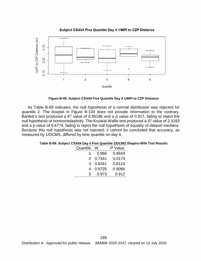
289 Distribution A: Approved for public release. 88ABW-2020-2247, cleared on 13 July 2020
Figure B-99. Subject CSA04 Five Quantile Day 4 1/MPI to CZP Distance
As Table B-89 indicates, the null hypothesis of a normal distribution was rejected for quantile 2. The boxplot in Figure B-100 does not provide information to the contrary. Bartlett’s test produced a K2 value of 0.95186 and a p value of 0.917, failing to reject the null hypothesis of homoscedasticity. The Kruskal-Wallis test produced a Χ2 value of 2.3183 and a p value of 0.6774, failing to reject the null hypothesis of equality of dataset medians. Because this null hypothesis was not rejected, it cannot be concluded that accuracy, as measured by 1/DCMS, differed by time quantile on day 4.
Table B-89. Subject CSA04 Day 4 Five Quantile 1/DCMS Shapiro-Wilk Test Results Quantile W P-Value
1 0.966 0.8644 2 0.7441 0.0174 3 0.9341 0.6124 4 0.9725 0.9086 5 0.973 0.912
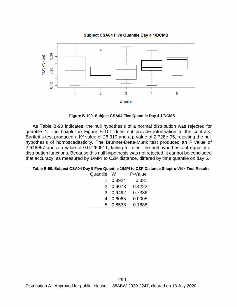
290 Distribution A: Approved for public release. 88ABW-2020-2247, cleared on 13 July 2020
Figure B-100. Subject CSA04 Five Quantile Day 4 1/DCMS
As Table B-90 indicates, the null hypothesis of a normal distribution was rejected for quantile 4. The boxplot in Figure B-101 does not provide information to the contrary. Bartlett’s test produced a K2 value of 26.319 and a p value of 2.728e-05, rejecting the null hypothesis of homoscedasticity. The Brunner-Dette-Munk test produced an F value of 2.646997 and a p value of 0.07260911, failing to reject the null hypothesis of equality of distribution functions. Because this null hypothesis was not rejected, it cannot be concluded that accuracy, as measured by 1/MPI to CZP distance, differed by time quantile on day 5.
Table B-90. Subject CSA04 Day 5 Five Quantile 1/MPI to CZP Distance Shapiro-Wilk Test Results Quantile W P-Value
1 0.8924 0.331 2 0.9078 0.4222 3 0.9492 0.7336 4 0.6065 0.0005 5 0.8538 0.1688
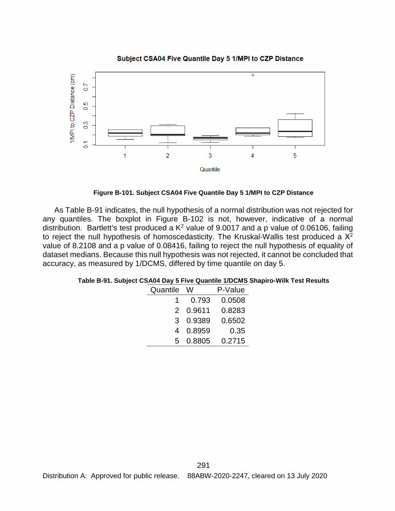
291 Distribution A: Approved for public release. 88ABW-2020-2247, cleared on 13 July 2020
Figure B-101. Subject CSA04 Five Quantile Day 5 1/MPI to CZP Distance
As Table B-91 indicates, the null hypothesis of a normal distribution was not rejected for any quantiles. The boxplot in Figure B-102 is not, however, indicative of a normal distribution. Bartlett’s test produced a K2 value of 9.0017 and a p value of 0.06106, failing to reject the null hypothesis of homoscedasticity. The Kruskal-Wallis test produced a Χ2 value of 8.2108 and a p value of 0.08416, failing to reject the null hypothesis of equality of dataset medians. Because this null hypothesis was not rejected, it cannot be concluded that accuracy, as measured by 1/DCMS, differed by time quantile on day 5.
Table B-91. Subject CSA04 Day 5 Five Quantile 1/DCMS Shapiro-Wilk Test Results Quantile W P-Value
1 0.793 0.0508 2 0.9611 0.8283 3 0.9389 0.6502 4 0.8959 0.35 5 0.8805 0.2715

292 Distribution A: Approved for public release. 88ABW-2020-2247, cleared on 13 July 2020
Figure B-102. Subject CSA04 Five Quantile Day 5 1/DCMS
As Table B-92 indicates, the null hypothesis of a normal distribution was rejected for quantile 4. The boxplot in Figure B-103 does not provide information to the contrary. Bartlett’s test produced a K2 value of 10.43 and a p value of 0.06392, failing to reject the null hypothesis of homoscedasticity. The Kruskal-Wallis test produced a Χ2 value of 6.2181 and a p value of 0.2856, failing to reject the null hypothesis of equality of dataset medians. Because this null hypothesis was not rejected, it cannot be concluded that accuracy, as measured by 1/MPI to CZP distance, differed by time quantile on day 2.
Table B-92. Subject CSA04 Day 2 Six Quantile 1/MPI to CZP Distance Shapiro-Wilk Test Results Quantile W P-Value
1 0.7792 0.0543 2 0.8993 0.4059 3 0.8056 0.0899 4 0.6828 0.0063 5 0.8757 0.2905 6 0.8627 0.2381

293 Distribution A: Approved for public release. 88ABW-2020-2247, cleared on 13 July 2020
Figure B-103. Subject CSA04 Day 2 Six Quantile 1/MPI to CZP Distance
As Table B-93 indicates, the null hypothesis of a normal distribution was rejected for quantiles 4 and 5. The boxplot in Figure B-104 does not provide information to the contrary. Bartlett’s test produced a K2 value of 3.7629 and a p value of 0.584, failing to reject the null hypothesis of homoscedasticity. The Kruskal-Wallis test produced a Χ2 value of 6.3419 and a p value of 0.2744, failing to reject the null hypothesis of equality of dataset medians. Because this null hypothesis was not rejected, it cannot be concluded that accuracy, as measured by 1/DCMS, differed by time quantile on day 2.
Table B-93. Subject CSA04 Day 2 Six Quantile 1/DCMS Shapiro-Wilk Test Results Quantile W P-Value
1 0.827 0.1321 2 0.8648 0.2459 3 0.9275 0.5797 4 0.7049 0.0108 5 0.7331 0.0206 6 0.9081 0.4563

294 Distribution A: Approved for public release. 88ABW-2020-2247, cleared on 13 July 2020
Figure B-104. Subject CSA04 Day 2 Six Quantile 1/DCMS
As Table B-94 indicates, the null hypothesis of a normal distribution was rejected for quantiles 2, 4 and 5. The boxplot in Figure B-105 does not provide information to the contrary. Bartlett’s test produced a K2 value of 19.587 and a p value of 0.001493, rejecting the null hypothesis of homoscedasticity. The Brunner-Dette-Munk test produced an F value of 1.406089 and a p value of 0.2724887, failing to reject the null hypothesis of equality of distribution functions. Because this null hypothesis was not rejected, it cannot be concluded that accuracy, as measured by 1/MPI to CZP distance, differed by time quantile on day 3.
Table B-94. Subject CSA04 Day 3 Six Quantile 1/MPI to CZP Distance Shapiro-Wilk Test Results Quantile W P-Value
1 0.8633 0.2403 2 0.6362 0.0018 3 0.8543 0.2084 4 0.7573 0.0347 5 0.6372 0.0019 6 0.8624 0.2688
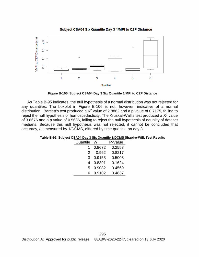
295 Distribution A: Approved for public release. 88ABW-2020-2247, cleared on 13 July 2020
Figure B-105. Subject CSA04 Day 3 Six Quantile 1/MPI to CZP Distance
As Table B-95 indicates, the null hypothesis of a normal distribution was not rejected for any quantiles. The boxplot in Figure B-106 is not, however, indicative of a normal distribution. Bartlett’s test produced a K2 value of 2.8862 and a p value of 0.7175, failing to reject the null hypothesis of homoscedasticity. The Kruskal-Wallis test produced a Χ2 value of 3.8676 and a p value of 0.5686, failing to reject the null hypothesis of equality of dataset medians. Because this null hypothesis was not rejected, it cannot be concluded that accuracy, as measured by 1/DCMS, differed by time quantile on day 3.
Table B-95. Subject CSA04 Day 3 Six Quantile 1/DCMS Shapiro-Wilk Test Results Quantile W P-Value
1 0.8672 0.2553 2 0.962 0.8217 3 0.9153 0.5003 4 0.8391 0.1624 5 0.9082 0.4569 6 0.9102 0.4837

296 Distribution A: Approved for public release. 88ABW-2020-2247, cleared on 13 July 2020
Figure B-106. Subject CSA04 Day 3 Six Quantile 1/DCMS
As Table B-96 indicates, the null hypothesis of a normal distribution was not rejected for any quantiles. The boxplot in Figure B-107 is not, however, indicative of a normal distribution. Bartlett’s test produced a K2 value of 2.4544 and a p value of 0.7833, failing to reject the null hypothesis of homoscedasticity. The Kruskal-Wallis test produced a Χ2 value of 3.3071 and a p value of 0.6528, failing to reject the null hypothesis of equality of dataset medians. Because this null hypothesis was not rejected, it cannot be concluded that accuracy, as measured by 1/MPI to CZP distance, differed by time quantile on day 4.
Table B-96. Subject CSA04 Six Quantile Day 4 1/MPI to CZP Distance Shapiro-Wilk Test Results Quantile W P-Value
1 0.9843 0.9562 2 0.8841 0.3282 3 0.989 0.976 4 0.9482 0.724 5 0.9229 0.549 6 0.9938 0.9911

297 Distribution A: Approved for public release. 88ABW-2020-2247, cleared on 13 July 2020
Figure B-107. Subject CSA04 Six Quantile Day 4 1/MPI to CZP Distance Shapiro-Wilk Test Results
As Table B-97 indicates, the null hypothesis of a normal distribution was not rejected for any quantiles. The boxplot in Figure B-108 is not, however, indicative of a normal distribution. Bartlett’s test produced a K2 value of 8.5213 and a p value of 0.1298, failing to reject the null hypothesis of homoscedasticity. The Kruskal-Wallis test produced a Χ2 value of 3.7406 and a p value of 0.5873, failing to reject the null hypothesis of equality of dataset medians. Because this null hypothesis was not rejected, it cannot be concluded that accuracy, as measured by 1/DCMS, differed by time quantile on day 4.
Table B-97. Subject CSA04 Six Quantile Day 4 1/DCMS Shapiro-Wilk Test Results Quantile W P-Value
1 0.8672 0.2553 2 0.962 0.8217 3 0.9153 0.5003 4 0.8391 0.1624 5 0.9082 0.4569 6 0.9102 0.4837
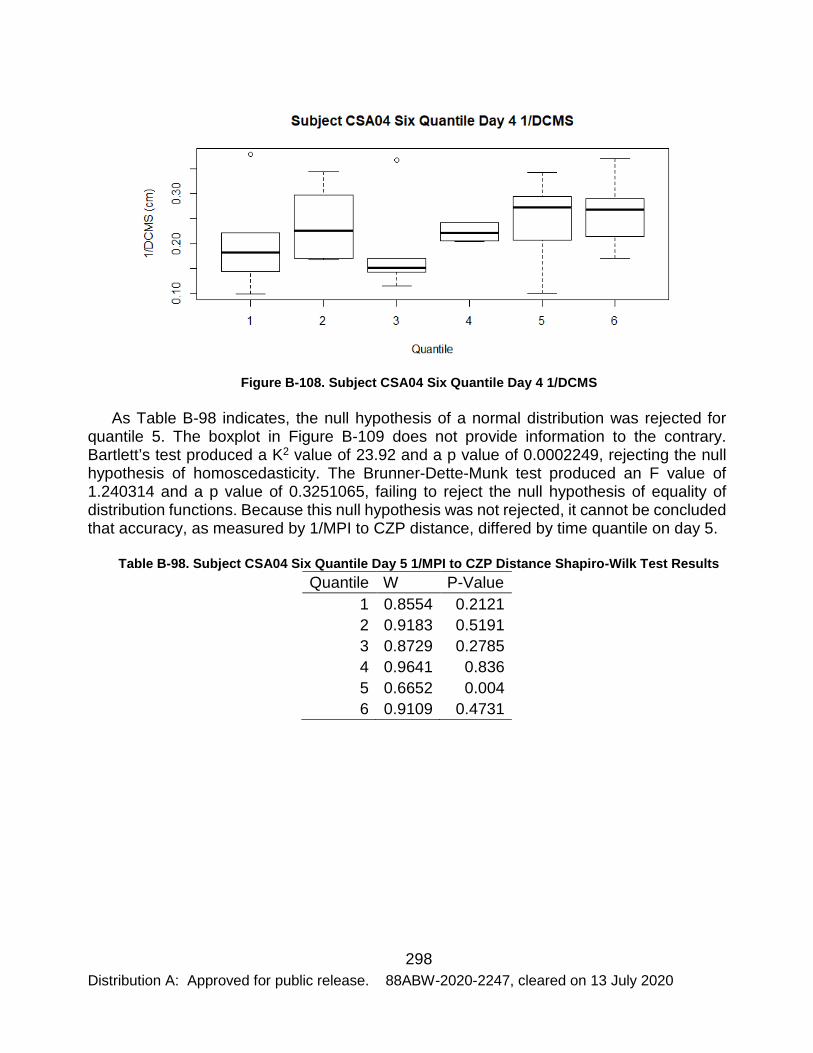
298 Distribution A: Approved for public release. 88ABW-2020-2247, cleared on 13 July 2020
Figure B-108. Subject CSA04 Six Quantile Day 4 1/DCMS
As Table B-98 indicates, the null hypothesis of a normal distribution was rejected for quantile 5. The boxplot in Figure B-109 does not provide information to the contrary. Bartlett’s test produced a K2 value of 23.92 and a p value of 0.0002249, rejecting the null hypothesis of homoscedasticity. The Brunner-Dette-Munk test produced an F value of 1.240314 and a p value of 0.3251065, failing to reject the null hypothesis of equality of distribution functions. Because this null hypothesis was not rejected, it cannot be concluded that accuracy, as measured by 1/MPI to CZP distance, differed by time quantile on day 5.
Table B-98. Subject CSA04 Six Quantile Day 5 1/MPI to CZP Distance Shapiro-Wilk Test Results Quantile W P-Value
1 0.8554 0.2121 2 0.9183 0.5191 3 0.8729 0.2785 4 0.9641 0.836 5 0.6652 0.004 6 0.9109 0.4731

299 Distribution A: Approved for public release. 88ABW-2020-2247, cleared on 13 July 2020
Figure B-109. Subject CSA04 Six Quantile Day 5 1/MPI to CZP Distance
As Table B-99 indicates, the null hypothesis of a normal distribution was not rejected for any quantiles. The boxplot in Figure B-110 is not, however, indicative of a normal distribution. Bartlett’s test produced a K2 value of 5.9849 and a p value of 0.3077, failing to reject the null hypothesis of homoscedasticity. The Kruskal-Wallis test produced a Χ2 value of 5.935 and a p value of 0.3478, failing to reject the null hypothesis of equality of dataset medians. Because this null hypothesis was not rejected, it cannot be concluded that accuracy, as measured by 1/DCMS, differed by time quantile on day 5.
Table B-99. Subject CSA04 Six Quantile Day 5 1/DCMS Shapiro-Wilk Test Results Quantile W P-Value
1 0.8432 0.174 2 0.9363 0.64 3 0.9178 0.5161 4 0.8139 0.1048 5 0.8499 0.1942 6 0.9274 0.5789

300 Distribution A: Approved for public release. 88ABW-2020-2247, cleared on 13 July 2020
Figure B-110. Subject CSA04 Six Quantile Day 5 1/DCMS
6.3.3 Quantile Analysis
As Table B-100 indicates, the null hypothesis of a normal distribution was rejected for day 2. The boxplot in Figure B-111 is not in agreement, but does not provide strong support for a normal distribution for all datasets. Bartlett’s test produced a K2 value of 3.0844 and a p value of 0.3788, failing to reject the null hypothesis of homoscedasticity. The Kruskal-Wallis test produced a Χ2 value of 3.0867 and a p value of 0.3785, failing to reject the null hypothesis of equality of dataset medians. Because this null hypothesis was not rejected, it cannot be concluded that accuracy, as measured by the first quantile of 1/MPI to CZP distance changed over the 4 days of firing.
Table B-100. Subject CSA04 Quantile 1 of 5 1/MPI to CZP Distance Shapiro-Wilk Test Results Day W P-Value
2 0.76501 0.02783 3 0.92128 0.51464 4 0.99668 0.99918 5 0.89241 0.33101

301 Distribution A: Approved for public release. 88ABW-2020-2247, cleared on 13 July 2020
Figure B-111. Subject CSA04 Quantile 1 of 5 1/MPI to CZP Distance
As Table B-101 indicates, the null hypothesis of a normal distribution was not rejected for any days. The boxplot in Figure B-112 is not, however, indicative of a normal distribution. Bartlett’s test produced a K2 value of 25.017 and a p value of 1.532e-05, rejecting the null hypothesis of homoscedasticity. The Brunner-Dette-Munk test produced an F value of 5.665773 and a p value of 0.00850945, rejecting the null hypothesis of equality of distribution functions. Because this null hypothesis was rejected, it can be concluded that accuracy, as measured by the second quantile of 1/MPI to CZP distance changed over the 4 days of firing. As Table B-102 shows, day 3’s 1/MPI to CZP distance for this quantile was significantly greater than the other days.
Table B-101. Subject CSA04 Quantile 2 of 5 1/MPI to CZP Distance Shapiro-Wilk Test Results Day W P-Value
2 0.95566 0.78577 3 0.80128 0.06035 4 0.89159 0.32659 5 0.90782 0.42219

302 Distribution A: Approved for public release. 88ABW-2020-2247, cleared on 13 July 2020
Figure B-112. Subject CSA04 Quantile 2 of 5 1/MPI to CZP Distance Table B-102. Subject CSA04 Quantile 2 of 5 1/MPI to CZP Distance REGWQ Test Results
Days Statistic Adj. P-Value CI
2 & 3 4.3641 0.0274 0.2909 2 & 4 0.3241 0.9715 0.0216 2 & 5 0.099 0.9449 0.0066 3 & 4 4.04 0.0098 0.2693 3 & 5 4.2651 0.0179 0.2843 4 & 5 0.2251 0.8751 0.015
As Table B-103 indicates, the null hypothesis of a normal distribution was not rejected for any days. The boxplot in Figure B-113 is not, however, indicative of a normal distribution. Bartlett’s test produced a K2 value of 25.94 and a p value of 9.815e-06, rejecting the null hypothesis of homoscedasticity. The Brunner-Dette-Munk test produced an F value of 5.718901 and a p value of 0.01520875, rejecting the null hypothesis of equality of distribution functions. Because this null hypothesis was rejected, it can be concluded that accuracy, as measured by the third quantile of 1/MPI to CZP distance changed over the 4 days of firing. As Figure B-113 and Table B-104 show, day 3’s 1/MPI to CZP distance for this quantile was significantly greater than days 4 and 5.
Table B-103. Subject CSA04 Quantile 3 of 5 1/MPI to CZP Distance Shapiro-Wilk Test Results Day W P-Value
2 0.89709 0.35699

303 Distribution A: Approved for public release. 88ABW-2020-2247, cleared on 13 July 2020
3 0.9127 0.45438 4 0.97411 0.91881 5 0.94918 0.7336
Figure B-113. Subject CSA04 Quantile 3 of 5 1/MPI to CZP Distance Table B-104. Subject CSA04 Quantile 3 of 5 1/MPI to CZP Distance REGWQ Test Results
Days
Test Stat.
Adj. P-Value
Conf. Int.
2 3 2.8093 0.0609 0.2598 2 4 1.5763 0.2782 0.1458 2 5 2.1972 0.2883 0.2032 3 4 4.3856 0.0149 0.4056 3 5 5.0065 0.0102 0.4631 4 5 0.6209 0.6653 0.0574
As Table B-105 indicates, the null hypothesis of a normal distribution was rejected for days 2, 3 and 5. The boxplot in Figure B-114 does not provide information to the contrary. Bartlett’s test produced a K2 value of 29.496 and a p value of 1.761e-06, rejecting the null hypothesis of homoscedasticity. The Brunner-Dette-Munk test produced an F value of 0.5006752 and a p value of 0.6844, failing to reject the null hypothesis of equality of distribution functions. Because this null hypothesis was not rejected, it cannot be concluded that accuracy, as measured by the fourth quantile of 1/MPI to CZP distance changed over the 4 days of firing.
Table B-105. Subject CSA04 Quantile 4 of 5 1/MPI to CZP Distance Shapiro-Wilk Test Results Day W P-Value
2 0.78707 0.044824 3 0.54509 9.42E-05 4 0.88983 0.317319

304 Distribution A: Approved for public release. 88ABW-2020-2247, cleared on 13 July 2020
5 0.60655 0.00055
Figure B-114. Subject CSA04 Quantile 4 of 5 1/MPI to CZP Distance
As Table B-106 indicates, the null hypothesis of a normal distribution was not rejected for any days. The boxplot in Figure B-115 is not, however, indicative of a normal distribution. Bartlett’s test produced a K2 value of 39.845 and a p value of 1.149e-08, rejecting the null hypothesis of homoscedasticity. The Brunner-Dette-Munk test produced an F value of 4.949106 and a p value of 0.01619872, rejecting the null hypothesis of equality of distribution functions. Because this null hypothesis not rejected, it can be concluded that accuracy, as measured by the fifth quantile of 1/MPI to CZP distance changed over the 4 days of firing. As shown in Table B-107, day 3 has a significantly greater 1/MPI to CZP distance than days 2, 4 and 5.
Table B-106. Subject CSA04 Quantile 5 of 5 1/MPI to CZP Distance Shapiro-Wilk Test Results Day W P-Value
2 0.84567 0.14514 3 0.79944 0.08018 4 0.96661 0.86896 5 0.85376 0.16876

305 Distribution A: Approved for public release. 88ABW-2020-2247, cleared on 13 July 2020
Figure B-115. Subject CSA04 Quantile 5 of 5 1/MPI to CZP Distance Table B-107. Subject CSA04 Quantile 5 of 5 1/MPI to CZP Distance REGWQ Test Results
Days Statistic Adj. P-Value CI
2 & 3 4.1318 0.0088 0.7815 2 & 4 0.5 0.9337 0.0902 2 & 5 0.2045 0.8865 0.0369 3 & 4 4.6086 0.0197 0.8717 3& 5 4.3268 0.0169 0.8184 4 & 5 0.2955 0.8367 0.0533
As Table B-108 indicates, the null hypothesis of a normal distribution was rejected for day 2. The boxplot in Figure B-116 does not provide information to the contrary. Bartlett’s test produced a K2 value of 1.3562 and a p value of 0.7158, failing to reject the null hypothesis of homoscedasticity. The Kruskal-Wallis test produced a Χ2 value of 2.7133 and a p value of 0.438, failing to reject the null hypothesis of equality of dataset medians. Because this null hypothesis not rejected, it can be concluded that accuracy, as measured by the first quantile of 1/DCMS did not change over the 4 days of firing.
Table B-108. Subject CSA04 Quantile 1 of 5 1/DCMS Shapiro-Wilk Test Results Day W P-Value
2 0.77468 0.03437 3 0.91673 0.4821 4 0.96597 0.86435 5 0.79303 0.05083

306 Distribution A: Approved for public release. 88ABW-2020-2247, cleared on 13 July 2020
Figure B-116. Subject CSA04 Quantile 1 of 5 1/DCMS
As Table B-109 indicates, the null hypothesis of a normal distribution was rejected for day 4. The boxplot in Figure B-117 does not provide information to the contrary. Bartlett’s test produced a K2 value of 1.967 and a p value of 0.5793, failing to reject the null hypothesis of homoscedasticity. The Kruskal-Wallis test produced a Χ2 value of 2.7467 and a p value of 0.4324, failing to reject the null hypothesis of equality of dataset medians. Because this null hypothesis not rejected, it can be concluded that accuracy, as measured by the second quantile of 1/DCMS did not change over the 4 days of firing.
Table B-109. Subject CSA04 Quantile 2 of 5 1/DCMS Shapiro-Wilk Test Results Day W P-Value
2 0.92786 0.5637 3 0.97781 0.94019 4 0.74414 0.01745 5 0.96112 0.82834

307 Distribution A: Approved for public release. 88ABW-2020-2247, cleared on 13 July 2020
Figure B-117. Subject CSA04 Quantile 2 of 5 1/DCMS
As Table B-110 indicates, the null hypothesis of a normal distribution was rejected for day 2. The boxplot in Figure B-118 does not provide information to the contrary. Bartlett’s test produced a K2 value of 11.358 and a p value of 0.009938, rejecting the null hypothesis of homoscedasticity. The Brunner-Dette-Munk test produced an F value of 0.4872991 and a p value of 0.6854672, failing to reject the null hypothesis of equality of distribution functions. Because this null hypothesis was not rejected, it can be concluded that accuracy, as measured by the third quantile of 1/DCMS did not change over the 4 days of firing.
Table B-110. Subject CSA04 Quantile 3 of 5 1/DCMS Shapiro-Wilk Test Results Day W P-Value
2 0.78743 0.04516 3 0.88461 0.29091 4 0.93414 0.61241 5 0.93888 0.65023

308 Distribution A: Approved for public release. 88ABW-2020-2247, cleared on 13 July 2020
Figure B-118. Subject CSA04 Quantile 3 of 5 1/DCMS
As Table B-111 indicates, the null hypothesis of a normal distribution was rejected for day 2. The boxplot in Figure B-119 does not provide information to the contrary. Bartlett’s test produced a K2 value of 3.8515 and a p value of 0.278, failing to reject the null hypothesis of homoscedasticity. The Kruskal-Wallis test produced a Χ2 value of 0.073333 and a p value of 0.9948, failing to reject the null hypothesis of equality of dataset medians. Because this null hypothesis was not rejected, it can be concluded that accuracy, as measured by the fourth quantile of 1/DCMS did not change over the 4 days of firing.
Table B-111. Subject CSA04 Quantile 4 of 5 1/DCMS Shapiro-Wilk Test Results Day W P-Value
2 0.74327 0.017104 3 0.86369 0.202193 4 0.97247 0.90857 5 0.89585 0.349982

309 Distribution A: Approved for public release. 88ABW-2020-2247, cleared on 13 July 2020
Figure B-119. Subject CSA04 Quantile 4 of 5 1/DCMS
As Table B-112 indicates, the null hypothesis of a normal distribution was not rejected for any days. The boxplot in Figure B-120 is not, however, indicative of a normal distribution. Bartlett’s test produced a K2 value of 6.8354 and a p value of 0.07733, failing to reject the null hypothesis of homoscedasticity. The Kruskal-Wallis test produced a Χ2 value of 2.1522 and a p value of 0.5414, failing to reject the null hypothesis of equality of dataset medians. Because this null hypothesis was not rejected, it can be concluded that accuracy, as measured by the fifth quantile of 1/DCMS did not change over the 4 days of firing.
Table B-112. Subject CSA04 Quantile 5 of 5 1/DCMS Shapiro-Wilk Test Results Day W P-Value
2 0.96129 0.8296 3 0.84595 0.18206 4 0.97301 0.912 5 0.88053 0.2715

310 Distribution A: Approved for public release. 88ABW-2020-2247, cleared on 13 July 2020
Figure B-120. Subject CSA04 Quantile 5 of 5 1/DCMS
As Table B-113 indicates, the null hypothesis of a normal distribution was not rejected for any days. The boxplot in Figure B-121 is not, however, indicative of a normal distribution. Bartlett’s test produced a K2 value of 1.8391 and a p value of 0.6065, failing to reject the null hypothesis of homoscedasticity. The Kruskal-Wallis test produced a Χ2 value of 3.0457 and a p value of 0.3846, failing to reject the null hypothesis of equality of dataset medians. Because this null hypothesis was not rejected, it can be concluded that accuracy, as measured by the first quantile of 1/MPI to CZP distance did not change over the 4 days of firing.
Table B-113. Subject CSA04 Quantile 1 of 6 1/MPI to CZP Distance Shapiro-Wilk Test Results Day W P-Value
2 0.77921 0.05427 3 0.86329 0.24032 4 0.9843 0.95624 5 0.85536 0.21207
311 Distribution A: Approved for public release. 88ABW-2020-2247, cleared on 13 July 2020
Figure B-121. Subject CSA04 Quantile 1 of 6 1/MPI to CZP Distance
As Table B-114 indicates, the null hypothesis of a normal distribution was rejected for day 3. The boxplot in Figure B-122 does not provide information to the contrary. Bartlett’s test produced a K2 value of 18.643 and a p value of 0.000324, rejecting the null hypothesis of homoscedasticity. The Brunner-Dette-Munk test produced an F value of 7.015785 and a p value of 0.006520171, rejecting the null hypothesis of equality of distribution functions. As Table B-115 shows, significant differences were found only between days 3 and 4.
Table B-114. Subject CSA04 Quantile 2 of 6 1/MPI to CZP Distance Shapiro-Wilk Test Results Day W P-Value
2 0.89929 0.40595 3 0.63625 0.00182 4 0.88407 0.32817 5 0.91831 0.51913

312 Distribution A: Approved for public release. 88ABW-2020-2247, cleared on 13 July 2020
Figure B-122. Subject CSA04 Quantile 2 of 6 1/MPI to CZP Distance Table B-115. Subject CSA04 Quantile 2 of 6 1/MPI to CZP Distance REGWQ Test Results
Days Statistic Adj. P-Value CI
2 & 3 3.7908 0.0704 0.298 2 & 4 0.6903 0.8779 0.0543 2 & 5 0.0264 0.9853 0.0021 3 & 4 3.1005 0.0435 0.2438 3 & 5 3.7645 0.05 0.296 4 & 5 0.6639 0.6451 0.0522
As Table B-116 indicates, the null hypothesis of a normal distribution was not rejected for any days. The boxplot in Figure B-123 is not, however, indicative of a normal distribution. Bartlett’s test produced a K2 value of 5.9618 and a p value of 0.1135, failing to reject the null hypothesis of homoscedasticity. The Kruskal-Wallis test produced a Χ2 value of 8.6571 and a p value of 0.03471, rejecting the null hypothesis of equality of dataset medians. Because this null hypothesis was rejected, it can be concluded that accuracy, as measured by the third quantile of 1/MPI to CZP distance changed over the 4 days of firing. As Table B-117 shows, there were significant differences between day 3 and days 4 and 5.
Table B-116. Subject CSA04 Quantile 3 of 6 1/MPI to CZP Distance Shapiro-Wilk Test Results Day W P-Value
2 0.80556 0.08987

313 Distribution A: Approved for public release. 88ABW-2020-2247, cleared on 13 July 2020
3 0.85427 0.2084 4 0.98897 0.97595 5 0.87294 0.27851
Figure B-123. Subject CSA04 Quantile 3 of 6 1/MPI to CZP Distance Table B-117. Subject CSA04 Quantile 3 of 6 1/MPI to CZP Distance Dunn's Test Results
Days Z P-Value 2 & 3 -0.8552 0.1962 2 & 4 1.38976 0.0823 2 & 5 1.71047 0.0436 3 & 4 2.24499 0.0124 3 & 5 2.56571 0.0051 4 & 5 0.32071 0.3742
As Table B-118 indicates, the null hypothesis of a normal distribution was rejected for days 2 and 3. The boxplot in Figure B-124 does not provide information to the contrary. Bartlett’s test produced a K2 value of 25.948 and a p value of 9.782e-06, rejecting the null hypothesis of homoscedasticity. The Brunner-Dette-Munk test produced an F value of 5.260056 and a p value of 0.02417996 rejecting the null hypothesis of equality of distribution functions. Because this null hypothesis was rejected, it can be concluded that accuracy, as measured by the fourth quantile of 1/MPI to CZP distance changed over the 4 days of firing. As Table B-119 shows, however, no statistically significant differences were found.
Table B-118. Subject CSA04 Quantile 4 of 6 1/MPI to CZP Distance Shapiro-Wilk Test Results Day W P-Value
2 0.68275 0.006266 3 0.75731 0.034735 4 0.94816 0.724011 5 0.96408 0.836037

314 Distribution A: Approved for public release. 88ABW-2020-2247, cleared on 13 July 2020
Figure B-124. Subject CSA04 Quantile 4 of 6 1/MPI to CZP Distance Table B-119. Subject CSA04 Quantile 4 of 6 1/MPI to CZP Distance REGWQ Test Results
Days Statistic Adj. P-Value CI
2 & 3 2.2747 0.1273 0.2731 2 & 4 0.129 0.9285 0.0155 2 & 5 0.9403 0.7867 0.1129 3 & 4 2.4037 0.2357 0.2886 3 & 5 3.215 0.1461 0.3859 4 & 5 0.8113 0.5742 0.0974
As Table B-120 indicates, the null hypothesis of a normal distribution was rejected for days 3 and 5. The boxplot in Figure B-125 does not provide information to the contrary. Bartlett’s test produced a K2 value of 17.909 and a p value of 0.0004593, rejecting the null hypothesis of homoscedasticity. The Brunner-Dette-Munk test produced an F value of 0.637486 and a p value of 0.5953076, failing to reject the null hypothesis of equality of dataset medians. Because this null hypothesis was not rejected, it cannot be concluded that accuracy, as measured by the fifth quantile of 1/MPI to CZP distance changed over the 4 days of firing.
Table B-120. Subject CSA04 Quantile 5 of 6 1/MPI to CZP Distance Shapiro-Wilk Test Results Day W P-Value
2 0.87574 0.29046 3 0.63721 0.00187 4 0.92292 0.54895 5 0.66521 0.004

315 Distribution A: Approved for public release. 88ABW-2020-2247, cleared on 13 July 2020
Figure B-125. Subject CSA04 Quantile 5 of 6 1/MPI to CZP Distance
As Table B-121 indicates, the null hypothesis of a normal distribution was not rejected for any days. The boxplot in Figure B-126 is not, however, indicative of a normal distribution. Bartlett’s test produced a K2 value of 31.904 and a p value of 5.482e-07, rejecting the null hypothesis of homoscedasticity. The Brunner-Dette-Munk test produced an F value of 4.920495 and a p value of 0.0200959 rejecting the null hypothesis of equality of distribution functions. Because this null hypothesis was rejected, it can be concluded that accuracy, as measured by the sixth quantile of 1/MPI to CZP distance changed over the 4 days of firing. As Table B-122 shows, there were significant differences between day 2 and days 3; 3 and 4 4 and 5.
Table B-121. Subject CSA04 Quantile 6 of 6 1/MPI to CZP Shapiro-Wilk Test Results Day W P-Value
2 0.86269 0.23808 3 0.86238 0.2688 4 0.99377 0.99109 5 0.91092 0.47314

316 Distribution A: Approved for public release. 88ABW-2020-2247, cleared on 13 July 2020
Figure B-126. Subject CSA04 Quantile 6 of 6 1/MPI to CZP Distance Table B-122. Subject CSA04 Quantile 6/6 1/MPI to CZP Distance REGWQ Test Results
Days Statistic Adj. P-Value CI
2 & 3 4.603 0.0139 0.9875 2 & 4 0.3013 0.8342 0.0609 2 & 5 0.0656 0.9636 0.0133 3 & 4 4.8871 0.0166 1.0484 3 & 5 4.5412 0.0058 0.9742 4 & 5 0.3669 0.9637 0.0742
As Table B-123 indicates, the null hypothesis of a normal distribution was not rejected for any days. The boxplot in Figure B-127 is not, however, indicative of a normal distribution. Bartlett’s test produced a K2 value of 0.93501 and a p value of 0.817, failing to reject the null hypothesis of homoscedasticity. The Kruskal-Wallis test produced a Χ2 value of 1.4686 and a p value of 0.6895, failing to reject the null hypothesis of equality of dataset medians. Because this null hypothesis was not rejected, it cannot be concluded that accuracy, as measured by the first quantile of 1/DCMS changed over the 4 days of firing.
Table B-123. Subject CSA04 Quantile 1 of 6 1/DCMS Shapiro-Wilk Test Results Day W P-Value
2 0.82703 0.13214 3 0.86722 0.25535 4 0.91035 0.4697 5 0.84322 0.17402

317 Distribution A: Approved for public release. 88ABW-2020-2247, cleared on 13 July 2020
Figure B-127. Subject CSA04 Quantile 1 of 6 1/DCMS
As Table B-124 indicates, the null hypothesis of a normal distribution was not rejected for any days. The boxplot in Figure B-128 is not, however, indicative of a normal distribution. Bartlett’s test produced a K2 value of 2.6483 and a p value of 0.4491, failing to reject the null hypothesis of homoscedasticity. The Kruskal-Wallis test produced a Χ2 value of 1.2629 and a p value of 0.738, failing to reject the null hypothesis of equality of dataset medians. Because this null hypothesis was not rejected, it cannot be concluded that accuracy, as measured by the second quantile of 1/DCMS changed over the 4 days of firing.
Table B-124. Subject CSA04 Quantile 2 of 6 1/DCMS Shapiro-Wilk Test Results Day W P-Value
2 0.86478 0.24594 3 0.96198 0.8217 4 0.89751 0.3963 5 0.93631 0.63999

318 Distribution A: Approved for public release. 88ABW-2020-2247, cleared on 13 July 2020
Figure B-128. Subject CSA04 Quantile 2 of 6 1/DCMS
As Table B-125 indicates, the null hypothesis of a normal distribution was rejected for day 4. The boxplot in Figure B-129 is not, however, indicative of a normal distribution. Bartlett’s test produced a K2 value of 0.98158 and a p value of 0.8057, failing to reject the null hypothesis of homoscedasticity. The Kruskal-Wallis test produced a Χ2 value of 4.8629 and a p value of 0.1821, failing to reject the null hypothesis of equality of dataset medians. Because this null hypothesis was not rejected, it cannot be concluded that accuracy, as measured by the third quantile of 1/DCMS changed over the 4 days of firing.
Table B-125. Subject CSA04 Quantile 3 of 6 1/DCMS Shapiro-Wilk Test Results Day W P-Value
2 0.92754 0.57972 3 0.91533 0.50026 4 0.74306 0.02563 5 0.91785 0.51615

319 Distribution A: Approved for public release. 88ABW-2020-2247, cleared on 13 July 2020
Figure B-129. Subject CSA04 Quantile 3 of 6 1/DCMS
As Table B-126 indicates, the null hypothesis of a normal distribution was rejected for day 2. The boxplot in Figure B-130 does not provide information to the contrary. Bartlett’s test produced a K2 value of 14.537 and a p value of 0.002259, rejecting the null hypothesis of homoscedasticity. The Brunner-Dette-Munk test produced an F value of 0.3613787 and a p value of 0.7538462, failing to reject the null hypothesis of equality of distribution functions. Because this null hypothesis was not rejected, it cannot be concluded that accuracy, as measured by the fourth quantile of 1/DCMS changed over the 4 days of firing.
Table B-126. Subject CSA04 Quantile 4 of 6 1/DCMS Shapiro-Wilk Test Results Day W P-Value
2 0.70488 0.010764 3 0.83906 0.162352 4 0.83889 0.1619 5 0.81394 0.10475

320 Distribution A: Approved for public release. 88ABW-2020-2247, cleared on 13 July 2020
Figure B-130. Subject CSA04 Quantile 4 of 6 1/DCMS
As Table B-127 indicates, the null hypothesis of a normal distribution was rejected for day 2. The boxplot in Figure B-131 does not provide information to the contrary. Bartlett’s test produced a K2 value of 3.3775 and a p value of 0.337, failing to reject the null hypothesis of homoscedasticity. The Kruskal-Wallis test produced a Χ2 value of 0.55429 and a p value of 0.9068, failing to reject the null hypothesis of equality of dataset medians. Because this null hypothesis was not rejected, it cannot be concluded that accuracy, as measured by the fifth quantile of 1/DCMS changed over the 4 days of firing.
Table B-127. Subject CSA04 Quantile 5 of 6 1/DCMS Shapiro-Wilk Test Results Day W P-Value
2 0.73313 0.02061 3 0.90821 0.4569 4 0.94489 0.7007 5 0.84991 0.19424

321 Distribution A: Approved for public release. 88ABW-2020-2247, cleared on 13 July 2020
Figure B-131. Subject CSA04 Quantile 5 of 6 1/DCMS
As Table B-128 indicates, the null hypothesis of a normal distribution was not rejected for any days. The boxplot in Figure B-132 is not, however, indicative of a normal distribution. Bartlett’s test produced a K2 value of 6.0155 and a p value of 0.1109, failing to reject the null hypothesis of homoscedasticity. The Kruskal-Wallis test produced a Χ2 value of 3.1263 and a p value of 0.3726, failing to reject the null hypothesis of equality of dataset medians. Because this null hypothesis was not rejected, it cannot be concluded that accuracy, as measured by the sixth quantile of 1/DCMS changed over the 4 days of firing.
Table B-128. Subject CSA04 Quantile 6 of 6 1/DCMS Shapiro-Wilk Test Results Day W P-Value
2 0.90811 0.45632 3 0.91024 0.4837 4 0.98411 0.9553 5 0.92742 0.57889

322 Distribution A: Approved for public release. 88ABW-2020-2247, cleared on 13 July 2020
Figure B-132. Subject CSA04 Quantile 6 of 6 1/DCMS
6.3.4 Correlation Results
In Table B-129, the results of the Pearson, Kendall, and Spearman tests for correlation between shot time and the distance from the shot to the center of the target are shown. As Table B-129 indicates, the respective null hypotheses of no correlation were not rejected for any days using any of the tests. As such, it cannot be concluded that there is a significant correlation between shot time and shot distance.
Table B-129. Subject CSA04 Correlation Results Pearson Kendall Spearman
Day T P-Value Coefficient Z P-Value Tau S P-Value Rho 2 -0.88478 0.3787 -0.0939 -0.54377 0.5866 -0.03905 129470 0.5381 -0.06575 3 -1.6998 0.09283 -0.18131 -1.0342 0.301 -0.07582 121330 0.3302 -0.10562 4 -0.75112 0.4546 -0.07981 -0.47063 0.6379 -0.03385 126550 0.6965 -0.04168 5 -1.6931 0.09398 -0.17761 -1.0214 0.3071 -0.07347 134450 0.3167 -0.10672
6.4 Subject CSA05 Results 6.4.1 IES Scoring Results
The MPI to CZP distance based IES results shown in Figure B-133 are indicative of similar trends for radii of 5 and 4 cm. The trend for 3 cm was similar to those trends, but was greater in amplitude. The trend for 2 cm had extreme changes due to the fact that no shot groups were within 2 cm of the center of the target on day 3 or day 5.
323 Distribution A: Approved for public release. 88ABW-2020-2247, cleared on 13 July 2020
Figure B-133. Subject CSA05 IES - MPI to CZP Distance Based
The MPI to CZP distance based RT results in Figure B-134 show very similar trends for radii from 5 to 3 cm, with the 5 cm data showing an overall decrease. The 2 cm data showed a trend of extreme changes caused by the fact that no shot groups were within 2 cm of the center of the target on days 3 and 5.
Figure B-134. Subject CSA05 RT – MPI to CZP Distance Based
MPI to CZP distance based proportion correct results, illustrated in Figure B-135, show more hits at greater radii, although the hit proportions for the 5 cm and 4 cm radii on day 3 are relatively close, due to the significant decrease in the 5 cm results. Overall, the trend among all radii was a decrease from day 2 to day 5.
0
20
40
60
80
100
120
140
160
180
Day 2 Day 3 Day 4 Day 5
IES
CSA05 IES - MPI to CZP Distance Based
5cm
4cm
3cm
2cm
0
1
2
3
4
5
6
Day 2 Day 3 Day 4 Day 5
RT (s
)
CSA05 RT - MPI to CZP Distance Based
5 cm
4 cm
3 cm
2 cm

324 Distribution A: Approved for public release. 88ABW-2020-2247, cleared on 13 July 2020
Figure B-135. Subject CSA05 Proportion Correct - MPI to CZP Distance Based
The DCMS based IES results, illustrated in Figure B-136, show similar trends for radii of 5 and 4 cm, while the 3 cm results show greater overall values and more extreme changes. The 2 cm results show extreme changes due to the fact that no shot groups were within 2 cm of the center of the target on days 3 and 5.
Figure B-136. Subject CSA05 IES – DCMS Based
The DCMS based RT results illustrated in Figure B-137 show similar trends for radii of 5 and 4 cm. The trend for 3 cm differs, showing a decrease followed by an increase from day 3 to day 5. The 2 cm results have extreme changes due to the fact that no shot groups were within 2 cm of the center of the target.
0
0.1
0.2
0.3
0.4
0.5
0.6
Day 2 Day 3 Day 4 Day 5
Prop
ortio
n Co
rrec
t
CSA05 Proportion Correct - MPI to CZP Distance Based
5 cm
4 cm
3 cm
2 cm
0
20
40
60
80
100
120
140
160
180
Day 2 Day 3 Day 4 Day 5
IES
CSA05 IES - DCMS Based
5cm
4cm
3cm
2cm

325 Distribution A: Approved for public release. 88ABW-2020-2247, cleared on 13 July 2020
Figure B-137. Subject CSA05 RT - DCMS Based
The DCMS based proportion correct results illustrated in Figure B-138 show similar patterns for the 5 cm and 4 cm radii. The 3 cm results show less extreme changes, while the 2 cm results were indicative of little change except for values of 0 on day 3 and day 5.
Figure B-138. Subject CSA05 Proportion Correct - DCMS Based
6.4.2 Conditional Accuracy Function Results
As Table B-130 indicates, the null hypothesis of a normal distribution was rejected for quantiles 1 and 4. The boxplot in Figure B-139 does not provide information to the contrary. Bartlett’s test produced a K2 value of 6.3617 and a p value of 0.1737, failing to reject the
0
1
2
3
4
5
6
Day 2 Day 3 Day 4 Day 5
RT (s
)
CSA05 RT - DCMS Based
5 cm
4 cm
3 cm
2 cm
0
0.1
0.2
0.3
0.4
0.5
0.6
0.7
Day 2 Day 3 Day 4 Day 5
Prop
ortio
n Co
rrec
t
CSA05 Proportion Correct - DCMS Based
5 cm
4 cm
3 cm
2 cm

326 Distribution A: Approved for public release. 88ABW-2020-2247, cleared on 13 July 2020
null hypothesis of homoscedasticity. The Kruskal-Wallis test produced a Χ2 value of 1.071 and a p value of 0.8989, failing to reject the null hypothesis of equality of dataset medians. Because this null hypothesis was not rejected, it cannot be concluded that accuracy, as measured by 1/MPI to CZP distance, differed by time quantile on day 2.
Table B-130. Subject CSA05 Day 2 Five Quantile 1/MPI to CZP Distance Shapiro-Wilk Test Results
Quantile W P-Value 1 0.7546 0.0221 2 0.8586 0.1843 3 0.8428 0.1374 4 0.735 0.0141 5 0.9484 0.7274
Figure B-139. Subject CSA05 Five Quantile Day 2 1/MPI to CZP Distance
As Table B-131 indicates, the null hypothesis of a normal distribution was rejected for quantiles 1 and 5. The boxplot in Figure B-140 does not provide information to the contrary. Bartlett’s test produced a K2 value of 7.0812 and a p value of 0.1317, failing to reject the null hypothesis of homoscedasticity. The Kruskal-Wallis test produced a Χ2 value of 4.4387 and a p value of 0.3499, failing to reject the null hypothesis of equality of dataset medians. Because this null hypothesis was not rejected, it cannot be concluded that accuracy, as measured by 1/DCMS, differed by time quantile on day 2.
Table B-131. Subject CSA05 Five Quantile Day 2 Five Quantile 1/DCMS Shapiro-Wilk Test Results Quantile W P-Value
1 0.7487 0.0193 2 0.9431 0.6841 3 0.9353 0.6214

327 Distribution A: Approved for public release. 88ABW-2020-2247, cleared on 13 July 2020
4 0.8798 0.2683 5 0.7878 0.0455
Figure B-140. Subject CSA05 Five Quantile Day 2 1/DCMS
As Table B-132 indicates, the null hypothesis of a normal distribution was rejected for quantiles 1 and 5. The boxplot in Figure B-141 does not provide information to the contrary. Bartlett’s test produced a K2 value of 8.6197 and a p value of 0.07134, failing to reject the null hypothesis of homoscedasticity. The Kruskal-Wallis test produced a Χ2 value of 8.2194 and a p value of 0.08387, failing to reject the null hypothesis of equality of dataset medians. Because this null hypothesis was not rejected, it cannot be concluded that accuracy, as measured by 1/MPI to CZP distance, differed by time quantile on day 3.
Table B-132. Subject CSA05 Five Quantile Day 3 1/MPI to CZP Distance Shapiro-Wilk Test Results Quantile W P-Value
1 0.7828 0.0409 2 0.93 0.5801 3 0.8157 0.081 4 0.8599 0.1889 5 0.7435 0.0172

328 Distribution A: Approved for public release. 88ABW-2020-2247, cleared on 13 July 2020
Figure B-141. Subject CSA05 Five Quantile Day 3 1/MPI to CZP Distance
As Table B-133 indicates, the null hypothesis of a normal distribution was not rejected for any quantiles. The boxplot in Figure B-142 is not, however, indicative of a normal distribution. Bartlett’s test produced a K2 value of 2.0189 and a p value of 0.7323, failing to reject the null hypothesis of homoscedasticity. The Kruskal-Wallis test produced a Χ2 value of 3.9527 and a p value of 0.4124, failing to reject the null hypothesis of equality of dataset medians. Because this null hypothesis was not rejected, it cannot be concluded that accuracy, as measured by 1/DCMS, differed by time quantile on day 3.
Table B-133. Subject CSA05 Five Quantile Day 3 1/DCMS Shapiro-Wilk Test Results Quantile W P-Value
1 0.8165 0.0822 2 0.9612 0.8291 3 0.9204 0.5084 4 0.8405 0.1316 5 0.831 0.1096

329 Distribution A: Approved for public release. 88ABW-2020-2247, cleared on 13 July 2020
Figure B-142. Subject CSA05 Five Quantile Day 3 1/DCMS
As Table B-134 indicates, the null hypothesis of a normal distribution was rejected for quantiles 1, 3 and 5. The boxplot in Figure B-143 does not provide information to the contrary. Bartlett’s test produced a K2 value of 7.0844 and a p value of 0.1315, failing to reject the null hypothesis of homoscedasticity. The Kruskal-Wallis test produced a Χ2 value of 3.686 and a p value of 0.4502, failing to reject the null hypothesis of equality of dataset medians. Because this null hypothesis was not rejected, it cannot be concluded that accuracy, as measured by 1/MPI to CZP distance, differed by time quantile on day 4.
Table B-134. Subject CSA05 Five Quantile Day 4 1/MPI to CZP Distance Shapiro-Wilk Test Results
Quantile W P-Value 1 0.7626 0.0264 2 0.8697 0.225 3 0.7907 0.0484 4 0.8704 0.2279 5 0.7707 0.0315

330 Distribution A: Approved for public release. 88ABW-2020-2247, cleared on 13 July 2020
Figure B-143. Subject CSA05 Five Quantile Day 4 1/MPI to CZP Distance
As Table B-135 indicates, the null hypothesis of a normal distribution was not rejected for any quantiles. The boxplot in Figure B-144 is not, however, indicative of a normal distribution. Bartlett’s test produced a K2 value of 7.3426 and a p value of 0.1189, failing to reject the null hypothesis of homoscedasticity. The Kruskal-Wallis test produced a Χ2 value of 2.7398 and a p value of 0.6023, failing to reject the null hypothesis of equality of dataset medians. Because this null hypothesis was not rejected, it cannot be concluded that accuracy, as measured by 1/DCMS, differed by time quantile on day 4.
Table B-135. Subject CSA05 Five Quantile Day 4 1/DCMS Shapiro-Wilk Test Results Quantile W P-Value
1 0.957294 0.798659 2 0.927353 0.55982 3 0.847831 0.151158 4 0.910643 0.440642 5 0.862223 0.196923
331 Distribution A: Approved for public release. 88ABW-2020-2247, cleared on 13 July 2020
Figure B-144. Subject CSA05 Five Quantile Day 4 1/DCMS
As Table B-136 indicates, the null hypothesis of a normal distribution was not rejected for any quantiles. The boxplot in Figure B-145 is not, however, indicative of a normal distribution. Bartlett’s test produced a K2 value of 9.062 and a p value of 0.0597, failing to reject the null hypothesis of homoscedasticity. The Kruskal-Wallis test produced a Χ2 value of 2.2753 and a p value of 0.6853, failing to reject the null hypothesis of equality of dataset medians. Because this null hypothesis was not rejected, it cannot be concluded that accuracy, as measured by 1/MPI to CZP distance, differed by time quantile on day 5.
Table B-136. Subject CSA05 Day 5 1/MPI to CZP Distance Shapiro-Wilk Test Results Quantile W P-Value
1 0.8985 0.365 2 0.8943 0.3414 3 0.9097 0.4344 4 0.9492 0.7336 5 0.9156 0.4745

332 Distribution A: Approved for public release. 88ABW-2020-2247, cleared on 13 July 2020
Figure B-145. Subject CSA05 Five Quantile Day 5 1/MPI to CZP Distance
As Table B-137 indicates, the null hypothesis of a normal distribution was not rejected for any quantiles. The boxplot in Figure B-146 is not, however, indicative of a normal distribution. Bartlett’s test produced a K2 value of 2.3775 and a p value of 0.6667, failing to reject the null hypothesis of homoscedasticity. The Kruskal-Wallis test produced a Χ2 value of 8.1333 and a p value of 0.08681, failing to reject the null hypothesis of equality of dataset medians. Because this null hypothesis was not rejected, it cannot be concluded that accuracy, as measured by 1/DCMS, differed by time quantile on day 5.
Table B-137. Subject CSA05 Five Quantile Day 5 1/DCMS Shapiro-Wilk Test Results Quantile W P-Value
1 0.8982 0.3632 2 0.8929 0.3338 3 0.8661 0.211 4 0.8722 0.2351 5 0.9714 0.9017
333 Distribution A: Approved for public release. 88ABW-2020-2247, cleared on 13 July 2020
Figure B-146. Subject CSA05 Five Quantile Day 5 1/DCMS
As Table B-138 indicates, the null hypothesis of a normal distribution was rejected for quantile 4. The boxplot in Figure B-147 does not provide information to the contrary. Bartlett’s test produced a K2 value of 9.635 and a p value of 0.08626, failing to reject the null hypothesis of homoscedasticity. The Kruskal-Wallis test produced a Χ2 value of 4.1381 and a p value of 0.5297, failing to reject the null hypothesis of equality of dataset medians. Because this null hypothesis was not rejected, it cannot be concluded that accuracy, as measured by 1/MPI to CZP distance, differed by time quantile on day 2.
Table B-138. Subject CSA05 Six Quantile Day 2 1/MPI to CZP Distance Shapiro-Wilk Test Results Quantile W P-Value
1 0.8049 0.0888 2 0.806 0.0906 3 0.8787 0.3036 4 0.6931 0.0081 5 0.8439 0.1759 6 0.8798 0.3084

334 Distribution A: Approved for public release. 88ABW-2020-2247, cleared on 13 July 2020
Figure B-147. Subject CSA05 Six Quantile Day 2 1/MPI to CZP Distance
As Table B-139 indicates, the null hypothesis of a normal distribution was rejected for quantile 1. The boxplot in Figure B-148 does not provide information to the contrary. Bartlett’s test produced a K2 value of 10.932 and a p value of 0.05274, failing to reject the null hypothesis of homoscedasticity. The Kruskal-Wallis test produced a Χ2 value of 7.8232 and a p value of 0.1663, failing to reject the null hypothesis of equality of dataset medians. Because this null hypothesis was not rejected, it cannot be concluded that accuracy, as measured by 1/DCMS, differed by time quantile on day 2.
Table B-139. Subject CSA05 Six Quantile Day 2 1/DCMS Shapiro-Wilk Test Results Quantile W P-Value
1 0.7443 0.0264 2 0.9565 0.7834 3 0.8959 0.3874 4 0.8476 0.1869 5 0.8878 0.3462 6 0.8487 0.1904

335 Distribution A: Approved for public release. 88ABW-2020-2247, cleared on 13 July 2020
Figure B-148. Subject CSA05 Six Quantile Day 2 1/DCMS
As Table B-140 indicates, the null hypothesis of a normal distribution was rejected for quantiles 3, 5 and 6. The boxplot in Figure B-149 does not provide information to the contrary. Bartlett’s test produced a K2 value of 5.694 and a p value of 0.3371, failing to reject the null hypothesis of homoscedasticity. The Kruskal-Wallis test produced a Χ2 value of 6.8477 and a p value of 0.2332, failing to reject the null hypothesis of equality of dataset medians. Because this null hypothesis was not rejected, it cannot be concluded that accuracy, as measured by 1/MPI to CZP distance, differed by time quantile on day 3.
Table B-140. Subject CSA05 Six Quantile Day 3 1/MPI to CZP Distance Shapiro-Wilk Test Results Quantile W P-Value
1 0.8191 0.1149 2 0.9049 0.4373 3 0.6888 0.0073 4 0.9398 0.6649 5 0.7099 0.0121 6 0.7519 0.031

336 Distribution A: Approved for public release. 88ABW-2020-2247, cleared on 13 July 2020
Figure B-149. Subject CSA05 Six Quantile Day 3 1/MPI to CZP Distance
As Table B-141 indicates, the null hypothesis of a normal distribution was rejected for quantile 6. The boxplot in Figure B-150 does not provide information to the contrary. Bartlett’s test produced a K2 value of 4.1164 and a p value of 0.5328, failing to reject the null hypothesis of homoscedasticity. The Kruskal-Wallis test produced a Χ2 value of 6.3574 and a p value of 0.273, failing to reject the null hypothesis of equality of dataset medians. Because this null hypothesis was not rejected, it cannot be concluded that accuracy, as measured by 1/DCMS, differed by time quantile on day 3.
Table B-141. Subject CSA05 Six Quantile Day 3 1/DCMS Shapiro-Wilk Test Results Quantile W P-Value
1 0.8683 0.2596 2 0.9497 0.7351 3 0.9016 0.419 4 0.9511 0.7449 5 0.8871 0.3429 6 0.7597 0.0365

337 Distribution A: Approved for public release. 88ABW-2020-2247, cleared on 13 July 2020
Figure B-150. Subject CSA05 Six Quantile Day 3 1/DCMS
As Table B-142 indicates, the null hypothesis of a normal distribution was rejected for quantile 3. The boxplot in Figure B-151 does not provide information to the contrary. Bartlett’s test produced a K2 value of 6.4759 and a p value of 0.2626, failing to reject the null hypothesis of homoscedasticity. The Kruskal-Wallis test produced a Χ2 value of 4.2413 and a p value of 0.5152, failing to reject the null hypothesis of equality of dataset medians. Because this null hypothesis was not rejected, it cannot be concluded that accuracy, as measured by 1/MPI to CZP distance, differed by time quantile on day 4.
Table B-142. Subject CSA05 Six Quantile Day 4 1/MPI to CZP Distance Shapiro-Wilk Test Results Quantile W P-Value
1 0.8248 0.1272 2 0.9992 0.9998 3 0.6399 0.002 4 0.9503 0.739 5 0.8077 0.0935 6 0.8117 0.1006

338 Distribution A: Approved for public release. 88ABW-2020-2247, cleared on 13 July 2020
Figure B-151. Subject CSA05 Six Quantile Day 4 1/MPI to CZP Distance
As Table B-143 indicates, the null hypothesis of a normal distribution was rejected for quantile 6. The boxplot in Figure B-152 does not provide information to the contrary. Bartlett’s test produced a K2 value of 7.2274 and a p value of 0.2043, failing to reject the null hypothesis of homoscedasticity. The Kruskal-Wallis test produced a Χ2 value of 1.6968 and a p value of 0.8893, failing to reject the null hypothesis of equality of dataset medians. Because this null hypothesis was not rejected, it cannot be concluded that accuracy, as measured by 1/DCMS, differed by time quantile on day 4.
Table B-143. Subject CSA05 Six Quantile Day 4 1/DCMS Shapiro-Wilk Test Results Quantile W P-Value
1 0.8683 0.2596 2 0.9497 0.7351 3 0.9016 0.419 4 0.9511 0.7449 5 0.8871 0.3429 6 0.7597 0.0365

339 Distribution A: Approved for public release. 88ABW-2020-2247, cleared on 13 July 2020
Figure B-152. Subject CSA05 Six Quantile Day 4 1/DCMS
As Table B-144 indicates, the null hypothesis of a normal distribution was not rejected for any quantiles. The boxplot in Figure B-153 is not, however, indicative of a normal distribution. Bartlett’s test produced a K2 value of 8.4847 and a p value of 0.1315, failing to reject the null hypothesis of homoscedasticity. The Kruskal-Wallis test produced a Χ2 value of 2.3161 and a p value of 0.8039, failing to reject the null hypothesis of equality of dataset medians. Because this null hypothesis was not rejected, it cannot be concluded that accuracy, as measured by 1/MPI to CZP distance, differed by time quantile on day 5.
Table B-144. Subject CSA05 Six Quantile Day 5 1/MPI to CZP Distance Shapiro-Wilk Test Results Quantile W P-Value
1 0.8661 0.2508 2 0.9408 0.6716 3 0.9868 0.9672 4 0.9356 0.635 5 0.9832 0.9509 6 0.9431 0.6878

340 Distribution A: Approved for public release. 88ABW-2020-2247, cleared on 13 July 2020
Figure B-153. Subject CSA05 Six Quantile Day 5 1/MPI to CZP Distance
As Table B-145 indicates, the null hypothesis of a normal distribution was not rejected for any quantiles. The boxplot in Figure B-154 is not, however, indicative of a normal distribution. Bartlett’s test produced a K2 value of 2.8789 and a p value of 0.7186, failing to reject the null hypothesis of homoscedasticity. The Kruskal-Wallis test produced a Χ2 value of 7.6426 and a p value of 0.1771, failing to reject the null hypothesis of equality of dataset medians. Because this null hypothesis was not rejected, it cannot be concluded that accuracy, as measured by 1/DCMS, differed by time quantile on day 5.
Table B-145. Subject CSA05 Six Quantile Day 5 1/DCMS Shapiro-Wilk Test Results Quantile W P-Value
1 0.8767 0.2948 2 0.8832 0.3242 3 0.8939 0.3769 4 0.9312 0.6043 5 0.9035 0.4292 6 0.9926 0.9881

341 Distribution A: Approved for public release. 88ABW-2020-2247, cleared on 13 July 2020
Figure B-154. Subject CSA05 Six Quantile Day 5 1/DCMS
6.4.3 Quantile Analysis
As Table B-146 indicates, the null hypothesis of a normal distribution was rejected for days 2, 3 and 4. The boxplot in Figure B-155 does not provide information to the contrary. Bartlett’s test produced a K2 value of 7.8333 and a p value of 0.04959, rejecting the null hypothesis of homoscedasticity. The Brunner-Dette-Munk test produced an F value of 1.207349 and a p value of 0.3339989, failing to reject the null hypothesis of equality of distribution functions. Because this null hypothesis was not rejected, it cannot be concluded that accuracy, as measured by the first quantile of 1/MPI to CZP distance changed over the 4 days of firing.
Table B-146. Subject CSA05 Quantile 1 of 5 1/MPI to CZP Distance Shapiro-Wilk Test Results Day W P-Value
2 0.75456 0.02207 3 0.78278 0.04091 4 0.76263 0.02641 5 0.89848 0.36502

342 Distribution A: Approved for public release. 88ABW-2020-2247, cleared on 13 July 2020
Figure B-155. Subject CSA05 Quantile 1 of 5 1/MPI to CZP Distance
As Table B-147 indicates, the null hypothesis of a normal distribution was not rejected for any days. The boxplot in Figure B-156 is not, however, indicative of a normal distribution. Bartlett’s test produced a K2 value of 9.161 and a p value of 0.02722, rejecting the null hypothesis of homoscedasticity. The Brunner-Dette-Munk test produced an F value of 3.054382 and a p value of 0.08327041, failing to reject the null hypothesis of equality of distribution functions. Because this null hypothesis was not rejected, it cannot be concluded that accuracy, as measured by the second quantile of 1/MPI to CZP distance changed over the 4 days of firing.
Table B-147. Subject CSA05 Quantile 2 of 5 1/MPI to CZP Distance Shapiro-Wilk Test Results Day W P-Value
2 0.85856 0.18427 3 0.93 0.58007 4 0.86971 0.22503 5 0.89431 0.34137

343 Distribution A: Approved for public release. 88ABW-2020-2247, cleared on 13 July 2020
Figure B-156. Subject CSA05 Quantile 2 of 5 1/MPI to CZP Distance
As Table B-148 indicates, the null hypothesis of a normal distribution was rejected for day 4. The boxplot in Figure B-157 does not provide information to the contrary. Bartlett’s test produced a K2 value of 5.318 and a p value of 0.1499, failing to reject the null hypothesis of homoscedasticity. The Kruskal-Wallis test produced a Χ2 value of 1.7133 and a p value of 0.634, failing to reject the null hypothesis of equality of distribution functions. Because this null hypothesis was not rejected, it cannot be concluded that accuracy, as measured by the third quantile of 1/MPI to CZP distance changed over the 4 days of firing.
Table B-148. Subject CSA05 Quantile 3 of 5 1/MPI to CZP Distance Shapiro-Wilk Test Results Day W P-Value
2 0.84278 0.13744 3 0.81572 0.08101 4 0.79073 0.04843 5 0.9097 0.4344

344 Distribution A: Approved for public release. 88ABW-2020-2247, cleared on 13 July 2020
Figure B-157. Subject CSA05 Quantile 3 of 5 1/MPI to CZP Distance
As Table B-149 indicates, the null hypothesis of a normal distribution was rejected for day 2. The boxplot in Figure B-158 does not provide information to the contrary. Bartlett’s test produced a K2 value of 6.612 and a p value of 0.08535 failing to reject the null hypothesis of homoscedasticity. The Kruskal-Wallis test produced a Χ2 value of 1.2333 and a p value of 0.745, failing to reject the null hypothesis of equality of dataset medians. Because this null hypothesis was not rejected, it cannot be concluded that accuracy, as measured by the fourth quantile of 1/MPI to CZP distance changed over the 4 days of firing.
Table B-149. Subject CSA05 Quantile 4 of 5 1/MPI to CZP Distance Shapiro-Wilk Test Results Day W P-Value
2 0.73495 0.01414 3 0.85992 0.18887 4 0.87041 0.22786 5 0.94918 0.7336

345 Distribution A: Approved for public release. 88ABW-2020-2247, cleared on 13 July 2020
Figure B-158. Subject CSA05 Quantile 4/5 1/MPI to CZP Distance
As Table B-150 indicates, the null hypothesis of a normal distribution was rejected for days 3 and 4. The boxplot in Figure B-159 does not provide information to the contrary. Bartlett’s test produced a K2 value of 1.3833 and a p value of 0.7095 failing to reject the null hypothesis of homoscedasticity. The Kruskal-Wallis test produced a Χ2 value of 1.7133 and a p value of 0.634, failing to reject the null hypothesis of equality of dataset medians. Because this null hypothesis was not rejected, it cannot be concluded that accuracy, as measured by the fifth quantile of 1/MPI to CZP distance changed over the 4 days of firing.
Table B-150. Quantile 5 of 5 1/MPI to CZP Distance Shapiro-Wilk Test Results Day W P-Value
2 0.94842 0.72744 3 0.74347 0.01718 4 0.77069 0.03152 5 0.91563 0.47446

346 Distribution A: Approved for public release. 88ABW-2020-2247, cleared on 13 July 2020
Figure B-159. Subject CSA05 Quantile 5 of 5 1/MPI to CZP Distance
As Table B-151 indicates, the null hypothesis of a normal distribution was rejected for day 2. The boxplot in Figure B-160 does not provide information to the contrary. Bartlett’s test produced a K2 value of 7.226 and a p value of 0.06503 failing to reject the null hypothesis of homoscedasticity. The Kruskal-Wallis test produced a Χ2 value of 4.9667 and a p value of 0.1743, failing to reject the null hypothesis of equality of dataset medians. Because this null hypothesis was not rejected, it cannot be concluded that accuracy, as measured by the first quantile of 1/DCMS changed over the 4 days of firing.
Table B-151. Subject CSA05 Quantile 1 of 5 1/DCMS Shapiro-Wilk Test Results Day W P-Value
2 0.7487 0.01934 3 0.81648 0.08225 4 0.95729 0.79866 5 0.89816 0.36317

347 Distribution A: Approved for public release. 88ABW-2020-2247, cleared on 13 July 2020
Figure B-160. Subject CSA05 Quantile 1 of 5 1/DCMS
As Table B-152 indicates, the null hypothesis of a normal distribution was not rejected for any days. The boxplot in Figure B-161 is not, however, strongly indicative of a normal distribution. Bartlett’s test produced a K2 value of 0.75445 and a p value of 0.8603 failing to reject the null hypothesis of homoscedasticity. The Kruskal-Wallis test produced a Χ2 value of 2.3667 and a p value of 0.4999, failing to reject the null hypothesis of equality of dataset medians. Because this null hypothesis was not rejected, it cannot be concluded that accuracy, as measured by the second quantile of 1/DCMS changed over the 4 days of firing.
Table B-152. Subject CSA05 Quantile 2 of 5 1/DCMS Shapiro-Wilk Test Results Day W P-Value
2 0.94308 0.6841 3 0.96123 0.82915 4 0.92735 0.55982 5 0.89292 0.33375

348 Distribution A: Approved for public release. 88ABW-2020-2247, cleared on 13 July 2020
Figure B-161. Subject CSA05 Quantile 2 of 5 1/DCMS
As Table B-153 indicates, the null hypothesis of a normal distribution was not rejected for any days. The boxplot in Figure B-162 is not, however, indicative of a normal distribution. Bartlett’s test produced a K2 value of 5.3402 and a p value of 0.1485 failing to reject the null hypothesis of homoscedasticity. The Kruskal-Wallis test produced a Χ2 value of 0.92667 and a p value of 0.819, failing to reject the null hypothesis of equality of dataset medians. Because this null hypothesis was not rejected, it cannot be concluded that accuracy, as measured by the third quantile of 1/DCMS changed over the 4 days of firing.
Table B-153. Subject CSA05 Quantile 3 of 5 1/DCMS Shapiro-Wilk Test Results Day W P-Value
2 0.93528 0.62143 3 0.92042 0.50842 4 0.84783 0.15116 5 0.86608 0.21103

349 Distribution A: Approved for public release. 88ABW-2020-2247, cleared on 13 July 2020
Figure B-162. Subject CAS05 Quantile 3 of 5 1/DCMS
As Table B-154 indicates, the null hypothesis of a normal distribution was not rejected for any days. The boxplot in Figure B-163 is not, however, indicative of a normal distribution. Bartlett’s test produced a K2 value of 0.74799 and a p value of 0.8619 failing to reject the null hypothesis of homoscedasticity. The Kruskal-Wallis test produced a Χ2 value of 2.5 and a p value of 0.4753, failing to reject the null hypothesis of equality of dataset medians. Because this null hypothesis was not rejected, it cannot be concluded that accuracy, as measured by the fourth quantile of 1/DCMS changed over the 4 days of firing.
Table B-154. Subject CSA05 Quantile 4 of 5 1/DCMS Shapiro-Wilk Test Results Day W P-Value
2 0.87983 0.26826 3 0.84049 0.13158 4 0.91064 0.44064 5 0.87218 0.23505

350 Distribution A: Approved for public release. 88ABW-2020-2247, cleared on 13 July 2020
Figure B-163. Subject CSA05 Quantile 4 of 5 1/DCMS
As Table B-155 indicates, the null hypothesis of a normal distribution was rejected for day 2. The boxplot in Figure B-164 does not provide information to the contrary. Bartlett’s test produced a K2 value of 4.6261 and a p value of 0.213 failing to reject the null hypothesis of homoscedasticity. The Kruskal-Wallis test produced a Χ2 value of 0.28667 and a p value of 0.9625, failing to reject the null hypothesis of equality of dataset medians. Because this null hypothesis was not rejected, it cannot be concluded that accuracy, as measured by the fifth quantile of 1/DCMS changed over the 4 days of firing.
Table B-155. Subject CSA05 Quantile 5 of 5 1/DCMS Shapiro-Wilk Test Results Day W P-Value
2 0.78778 0.0455 3 0.10957 0.10957 4 0.86222 0.19692 5 0.97139 0.90167

351 Distribution A: Approved for public release. 88ABW-2020-2247, cleared on 13 July 2020
Figure B-164. Subject CSA05 Quantile 5 of 5 1/DCMS
As Table B-156 indicates, the null hypothesis of a normal distribution was not rejected for any days. The boxplot in Figure B-165 is not, however, indicative of a normal distribution. Bartlett’s test produced a K2 value of 5.5883 and a p value of 0.1335 failing to reject the null hypothesis of homoscedasticity. The Kruskal-Wallis test produced a Χ2 value of 2.68 and a p value of 0.4436, failing to reject the null hypothesis of equality of dataset medians. Because this null hypothesis was not rejected, it cannot be concluded that accuracy, as measured by the first quantile of 1/MPI to CZP distance changed over the 4 days of firing.
Table B-156. Subject CSA05 Quantile 1 of 6 1/MPI to CZP Distance Shapiro-Wilk Test Results Day W P-Value
2 0.80488 0.08876 3 0.8191 0.11491 4 0.82483 0.12716 5 0.86606 0.25083
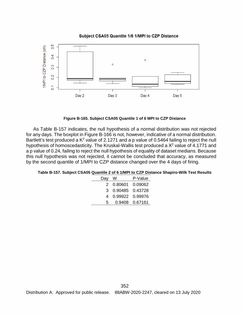
352 Distribution A: Approved for public release. 88ABW-2020-2247, cleared on 13 July 2020
Figure B-165. Subject CSA05 Quantile 1 of 6 MPI to CZP Distance
As Table B-157 indicates, the null hypothesis of a normal distribution was not rejected for any days. The boxplot in Figure B-166 is not, however, indicative of a normal distribution. Bartlett’s test produced a K2 value of 2.1271 and a p value of 0.5464 failing to reject the null hypothesis of homoscedasticity. The Kruskal-Wallis test produced a Χ2 value of 4.1771 and a p value of 0.24, failing to reject the null hypothesis of equality of dataset medians. Because this null hypothesis was not rejected, it cannot be concluded that accuracy, as measured by the second quantile of 1/MPI to CZP distance changed over the 4 days of firing.
Table B-157. Subject CSA05 Quantile 2 of 6 1/MPI to CZP Distance Shapiro-Wilk Test Results Day W P-Value
2 0.80601 0.09062 3 0.90485 0.43728 4 0.99922 0.99976 5 0.9408 0.67161
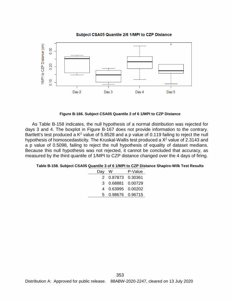
353 Distribution A: Approved for public release. 88ABW-2020-2247, cleared on 13 July 2020
Figure B-166. Subject CSA05 Quantile 2 of 6 1/MPI to CZP Distance
As Table B-158 indicates, the null hypothesis of a normal distribution was rejected for days 3 and 4. The boxplot in Figure B-167 does not provide information to the contrary. Bartlett’s test produced a K2 value of 5.8528 and a p value of 0.119 failing to reject the null hypothesis of homoscedasticity. The Kruskal-Wallis test produced a Χ2 value of 2.3143 and a p value of 0.5098, failing to reject the null hypothesis of equality of dataset medians. Because this null hypothesis was not rejected, it cannot be concluded that accuracy, as measured by the third quantile of 1/MPI to CZP distance changed over the 4 days of firing.
Table B-158. Subject CSA05 Quantile 3 of 6 1/MPI to CZP Distance Shapiro-Wilk Test Results Day W P-Value
2 0.87873 0.30361 3 0.68881 0.00729 4 0.63995 0.00202 5 0.98676 0.96715

354 Distribution A: Approved for public release. 88ABW-2020-2247, cleared on 13 July 2020
Figure B-167. Subject CSA05 Quantile 3 of 6 1/MPI to CZP Distance
As Table B-159 indicates, the null hypothesis of a normal distribution was rejected for day 2. The boxplot in Figure B-168 does not provide information to the contrary. Bartlett’s test produced a K2 value of 5.0622 and a p value of 0.1673 failing to reject the null hypothesis of homoscedasticity. The Kruskal-Wallis test produced a Χ2 value of 3.8686 and a p value of 0.276, failing to reject the null hypothesis of equality of dataset medians. Because this null hypothesis was not rejected, it cannot be concluded that accuracy, as measured by the fourth quantile of 1/MPI to CZP distance changed over the 4 days of firing.
Table B-159. Subject CSA05 Quantile 4 of 6 1/MPI to CZP Distance Shapiro-Wilk Test Results Day W P-Value
2 0.6931 0.0081 3 0.93985 0.66487 4 0.95026 0.73903 5 0.93559 0.63498

355 Distribution A: Approved for public release. 88ABW-2020-2247, cleared on 13 July 2020
Figure B-168. Subject CSA05 Quantile 4 of 6 1/MPI to CZP Distance
As Table B-160 indicates, the null hypothesis of a normal distribution was rejected for day 3. The boxplot in Figure B-169 does not provide information to the contrary. Bartlett’s test produced a K2 value of 7.328 and a p value of 0.0625 failing to reject the null hypothesis of homoscedasticity. The Kruskal-Wallis test produced a Χ2 value of 3.8914 and a p value of 0.2734, failing to reject the null hypothesis of equality of dataset medians. Because this null hypothesis was not rejected, it cannot be concluded that accuracy, as measured by the fifth quantile of 1/MPI to CZP distance changed over the 4 days of firing.
Table B-160. Subject CSA05 Quantile 5 of 6 1/MPI to CZP Distance Shapiro-Wilk Test Results Day W P-Value
2 0.84387 0.1759 3 0.70989 0.01212 4 0.80772 0.09354 5 0.98318 0.95089
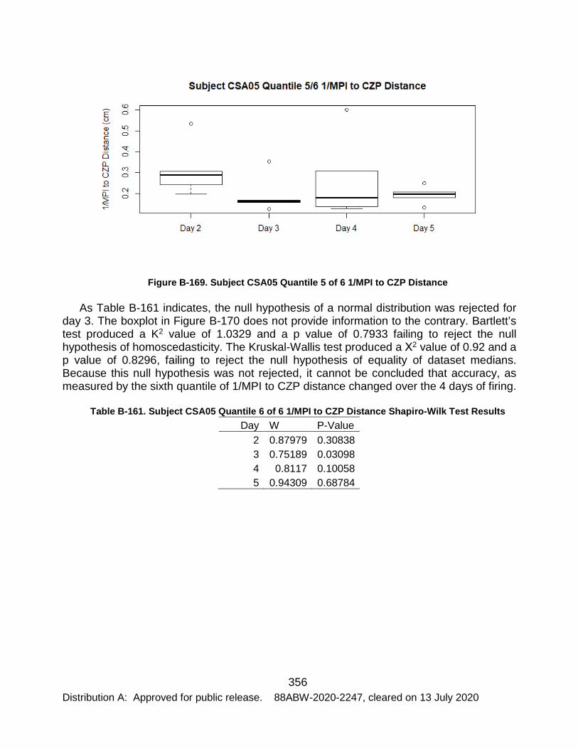
356 Distribution A: Approved for public release. 88ABW-2020-2247, cleared on 13 July 2020
Figure B-169. Subject CSA05 Quantile 5 of 6 1/MPI to CZP Distance
As Table B-161 indicates, the null hypothesis of a normal distribution was rejected for day 3. The boxplot in Figure B-170 does not provide information to the contrary. Bartlett’s test produced a K2 value of 1.0329 and a p value of 0.7933 failing to reject the null hypothesis of homoscedasticity. The Kruskal-Wallis test produced a Χ2 value of 0.92 and a p value of 0.8296, failing to reject the null hypothesis of equality of dataset medians. Because this null hypothesis was not rejected, it cannot be concluded that accuracy, as measured by the sixth quantile of 1/MPI to CZP distance changed over the 4 days of firing.
Table B-161. Subject CSA05 Quantile 6 of 6 1/MPI to CZP Distance Shapiro-Wilk Test Results Day W P-Value
2 0.87979 0.30838 3 0.75189 0.03098 4 0.8117 0.10058 5 0.94309 0.68784

357 Distribution A: Approved for public release. 88ABW-2020-2247, cleared on 13 July 2020
Figure B-170. Subject CSA05 Quantile 6 of 6 1/MPI to CZP Distance
As Table B-162 indicates, the null hypothesis of a normal distribution was rejected for day 2. The boxplot in Figure B-171 does not provide information to the contrary. Bartlett’s test produced a K2 value of 5.9855 and a p value of 0.1123 failing to reject the null hypothesis of homoscedasticity. The Kruskal-Wallis test produced a Χ2 value of 3.08 and a p value of 0.3795, failing to reject the null hypothesis of equality of dataset medians. Because this null hypothesis was not rejected, it cannot be concluded that accuracy, as measured by the first quantile of 1/DCMS changed over the 4 days of firing.
Table B-162. Subject CSA05 Quantile 1 of 6 1/DCMS Shapiro-Wilk Test Results Day W P-Value
2 0.74434 0.02636 3 0.8683 0.25962 4 0.90676 0.4484 5 0.87674 0.29482

358 Distribution A: Approved for public release. 88ABW-2020-2247, cleared on 13 July 2020
Figure B-171. Subject CSA05 Quantile 1 of 6 1/DCMS
As Table B-163 indicates, the null hypothesis of a normal distribution was not rejected for any days. The boxplot in Figure B-172 is not, however, indicative of a normal distribution. Bartlett’s test produced a K2 value of 0.47779 and a p value of 0.9237 failing to reject the null hypothesis of homoscedasticity. The Kruskal-Wallis test produced a Χ2 value of 8.1086 and a p value of 0.04382, rejecting the null hypothesis of equality of dataset medians. Because this null hypothesis was rejected, it can be concluded that accuracy, as measured by the second quantile of 1/DCMS changed over the 4 days of firing. As Table B-164 shows, the differences were between days 2 and 3 and days 3 and 4. While there were differences in dataset location, these differences were not indicative of a trend.
Table B-163. Subject CSA05 Quantile 2 of 6 1/DCMS Shapiro-Wilk Test Results Day W P-Value
2 0.9565 0.78341 3 0.94971 0.73515 4 0.9416 0.6773 5 0.88324 0.32424

359 Distribution A: Approved for public release. 88ABW-2020-2247, cleared on 13 July 2020
Figure B-172. Subject CSA05 Quantile 2 of 6 1/DCMS Table B-164. Subject CSA05 Quantile 2 of 6 1/DCMS Dunn's Test Results
Days Z P-Value 2 & 3 2.24499 0.0124 2 & 4 0 0.5 2 & 5 1.71047 0.0436 3 & 4 -2.245 0.0124 3 & 5 -0.5345 0.2965 4 & 5 1.71047 0.0436
As Table B-165 indicates, the null hypothesis of a normal distribution was not rejected for any days. The boxplot in Figure B-173 is not, however, indicative of a normal distribution. Bartlett’s test produced a K2 value of 0.34011 and a p value of 0.9523 failing to reject the null hypothesis of homoscedasticity. The Kruskal-Wallis test produced a Χ2 value of 1.9486 and a p value of 0.5831, failing to reject the null hypothesis of equality of dataset medians. Because this null hypothesis was not rejected, it cannot be concluded that accuracy, as measured by the third quantile of 1/DCMS changed over the 4 days of firing.
Table B-165. Subject CSA05 Quantile 3 of 6 1/DCMS Shapiro-Wilk Test Results Day W P-Value
2 0.89586 0.38743

360 Distribution A: Approved for public release. 88ABW-2020-2247, cleared on 13 July 2020
3 0.90164 0.41904 4 0.89618 0.3891 5 0.89387 0.37692
Figure B-173. Subject CSA05 Quantile 3 of 6 1/DCMS
As Table B-166 indicates, the null hypothesis of a normal distribution was not rejected for any days. The boxplot in Figure B-174 is not, however, indicative of a normal distribution. Bartlett’s test produced a K2 value of 3.2626 and a p value of 0.3529 failing to reject the null hypothesis of homoscedasticity. The Kruskal-Wallis test produced a Χ2 value of 1.3771 and a p value of 0.7109, failing to reject the null hypothesis of equality of dataset medians. Because this null hypothesis was not rejected, it cannot be concluded that accuracy, as measured by the fourth quantile of 1/DCMS changed over the 4 days of firing.
Table B-166. Subject CSA05 Quantile 4 of 6 1/DCMS Shapiro-Wilk Test Results Day W P-Value
2 0.84756 0.18694 3 0.95108 0.74491 4 0.87102 0.2706 5 0.93115 0.60426
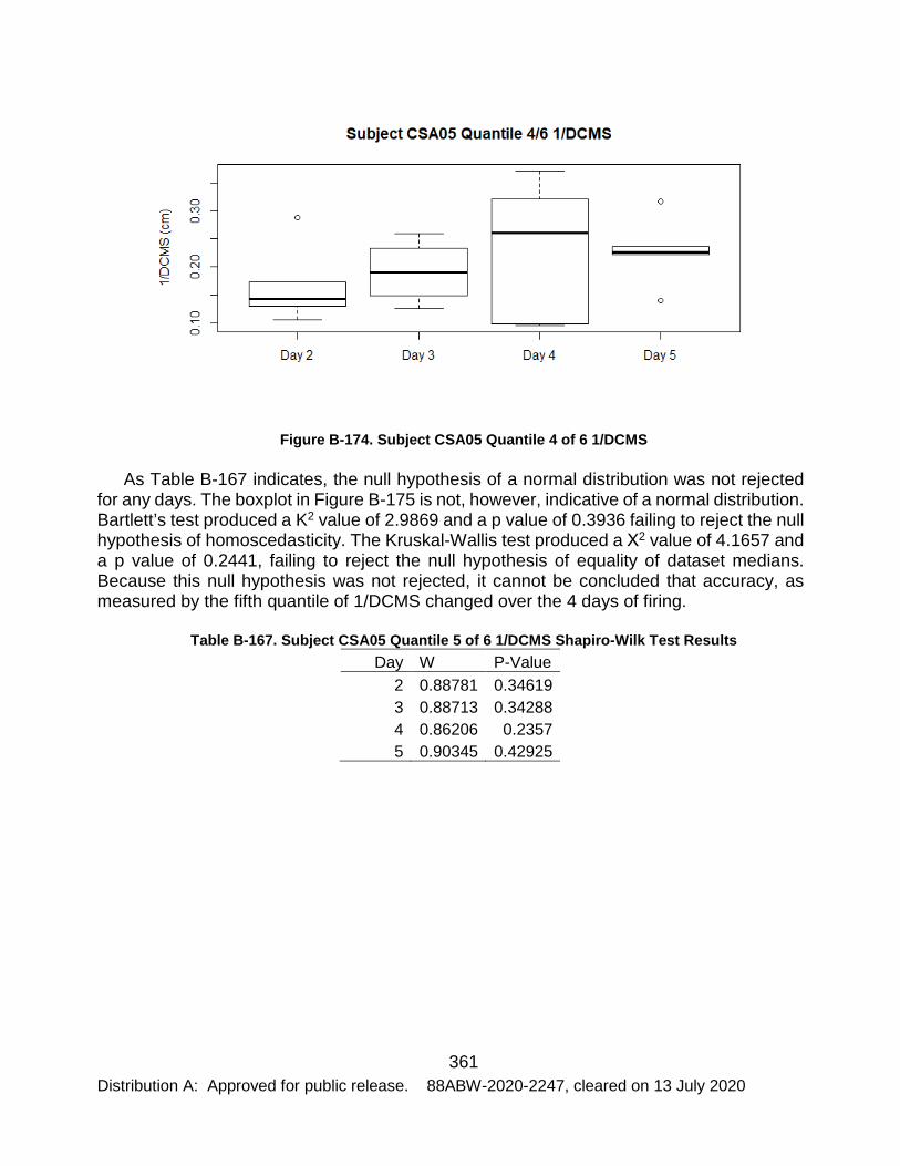
361 Distribution A: Approved for public release. 88ABW-2020-2247, cleared on 13 July 2020
Figure B-174. Subject CSA05 Quantile 4 of 6 1/DCMS
As Table B-167 indicates, the null hypothesis of a normal distribution was not rejected for any days. The boxplot in Figure B-175 is not, however, indicative of a normal distribution. Bartlett’s test produced a K2 value of 2.9869 and a p value of 0.3936 failing to reject the null hypothesis of homoscedasticity. The Kruskal-Wallis test produced a Χ2 value of 4.1657 and a p value of 0.2441, failing to reject the null hypothesis of equality of dataset medians. Because this null hypothesis was not rejected, it cannot be concluded that accuracy, as measured by the fifth quantile of 1/DCMS changed over the 4 days of firing.
Table B-167. Subject CSA05 Quantile 5 of 6 1/DCMS Shapiro-Wilk Test Results Day W P-Value
2 0.88781 0.34619 3 0.88713 0.34288 4 0.86206 0.2357 5 0.90345 0.42925

362 Distribution A: Approved for public release. 88ABW-2020-2247, cleared on 13 July 2020
Figure B-175. Subject CSA05 Quantile 5 of 6 1/DCMS
As Table B-168 indicates, the null hypothesis of a normal distribution was rejected for day 3. The boxplot in Figure B-176 is not, however, indicative of a normal distribution. Bartlett’s test produced a K2 value of 2.479 and a p value of 0.4791 failing to reject the null hypothesis of homoscedasticity. The Kruskal-Wallis test produced a Χ2 value of 0.48571 and a p value of 0.922, failing to reject the null hypothesis of equality of dataset medians. Because this null hypothesis was not rejected, it cannot be concluded that accuracy, as measured by the sixth quantile of 1/DCMS changed over the 4 days of firing.
Table B-168. Subject CSA05 Quantile 6 of 6 1/DCMS Shapiro-Wilk Test Results Day W P-Value
2 0.84869 0.19042 3 0.75967 0.03649 4 0.89148 0.3646 5 0.99264 0.98808
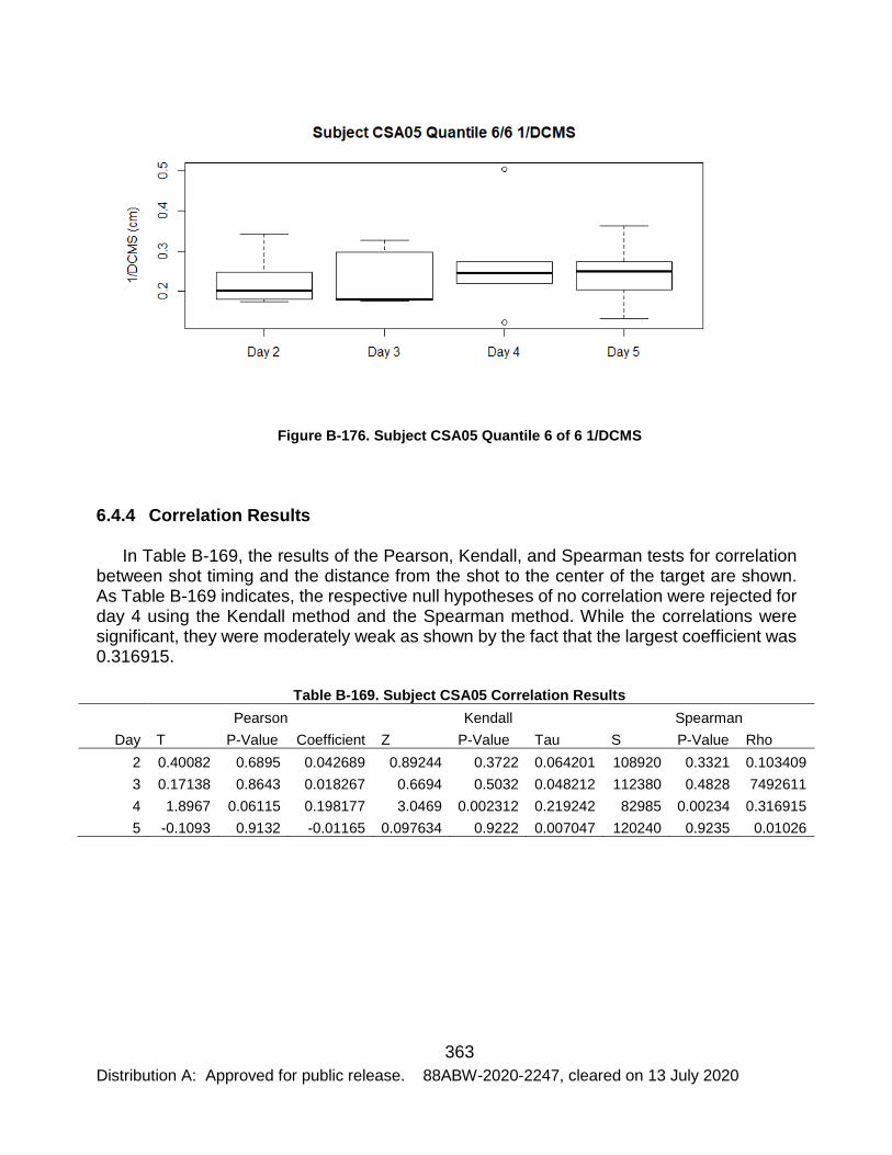
363 Distribution A: Approved for public release. 88ABW-2020-2247, cleared on 13 July 2020
Figure B-176. Subject CSA05 Quantile 6 of 6 1/DCMS
6.4.4 Correlation Results
In Table B-169, the results of the Pearson, Kendall, and Spearman tests for correlation between shot timing and the distance from the shot to the center of the target are shown. As Table B-169 indicates, the respective null hypotheses of no correlation were rejected for day 4 using the Kendall method and the Spearman method. While the correlations were significant, they were moderately weak as shown by the fact that the largest coefficient was 0.316915.
Table B-169. Subject CSA05 Correlation Results Pearson Kendall Spearman
Day T P-Value Coefficient Z P-Value Tau S P-Value Rho 2 0.40082 0.6895 0.042689 0.89244 0.3722 0.064201 108920 0.3321 0.103409 3 0.17138 0.8643 0.018267 0.6694 0.5032 0.048212 112380 0.4828 7492611 4 1.8967 0.06115 0.198177 3.0469 0.002312 0.219242 82985 0.00234 0.316915 5 -0.1093 0.9132 -0.01165 0.097634 0.9222 0.007047 120240 0.9235 0.01026

364 Distribution A: Approved for public release. 88ABW-2020-2247, cleared on 13 July 2020
APPENDIX C
6.1 Subject VS01 Data
As indicated in Table C-1, the null hypothesis of equality of proportions was not rejected for any of the visual acuities over the 3 days of firing. As indicated in Table C-2, Subject VS01’s performance at visual acuity A was lower than the other visual acuities on day 3 of firing, but the difference was not statistically significant. Hit proportions and 95% confidence intervals for each acuity over the days of firing are provided in Figures C-1 through C-4.
Table C-1. Subject VS01 Acuity Hit Proportions Acuity Day 2 Day 3 Day 4 Chi-Squared P-Value A 0.96875 0.875 0.90625 1.9091 0.385 B 1 0.90625 0.9375 2.9538 0.2283 C 0.9375 1 1 4.0851 0.1297 D 1 1 1 NA NA
Table C-2. Subject VS01 Daily Hit Proportions Day Acuity A Acuity B Acuity C Acuity D Chi-Squared P-Value
2 0.96875 1 0.9375 1 3.7547 0.2892 3 0.875 0.90625 1 1 7.7072 0.05247 4 0.90625 0.9375 1 1 5.6195 0.1317

365 Distribution A: Approved for public release. 88ABW-2020-2247, cleared on 13 July 2020
Figure C-1. Subject VS01 Acuity A Hit Proportions
Figure C-2. Subject VS01 Acuity B Hit Proportions
0
0.2
0.4
0.6
0.8
1
1.2
Hit P
ropo
rtio
ns
Subject VS01 Acuity A Hit Proportions with 95% Confidence Intervals
Day 2
Day 3
Day 4
0
0.2
0.4
0.6
0.8
1
1.2
Hit P
ropo
rtio
ns
Subject VS01 Acuity B Hit Proportions with 95% Confidence Intervals
Day 2
Day 3
Day 4

366 Distribution A: Approved for public release. 88ABW-2020-2247, cleared on 13 July 2020
Figure C-3. Subject VS01 Acuity C Hit Proportions
Figure C-4. Subject VS01 Acuity D Hit Proportions
6.2 Subject VS02 Data
As indicated in Table C-3, the null hypothesis of equality of proportions was not rejected for any of the visual acuities over the 4 days of firing. As indicated in Table C-4, Subject VS02’s performance did not differ to a significant extent at any of the visual acuities on any
0
0.2
0.4
0.6
0.8
1
1.2
Hit P
ropo
rtio
ns
Subject VS01 Acuity C Hit Proportions with 95% Confidence Intervals
Day 2
Day 3
Day 4
0.75
0.8
0.85
0.9
0.95
1
1.05
Hit P
ropo
rtio
ns
Subject VS01 Acuity D Hit Proportions with 95% Confidence Intervals
Day 2
Day 3
Day 4
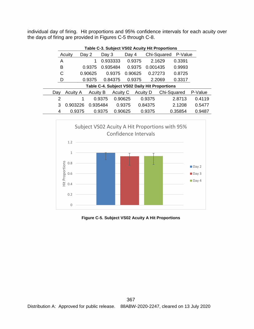
367 Distribution A: Approved for public release. 88ABW-2020-2247, cleared on 13 July 2020
individual day of firing. Hit proportions and 95% confidence intervals for each acuity over the days of firing are provided in Figures C-5 through C-8.
Table C-3. Subject VS02 Acuity Hit Proportions Acuity Day 2 Day 3 Day 4 Chi-Squared P-Value A 1 0.933333 0.9375 2.1629 0.3391 B 0.9375 0.935484 0.9375 0.001435 0.9993 C 0.90625 0.9375 0.90625 0.27273 0.8725 D 0.9375 0.84375 0.9375 2.2069 0.3317
Table C-4. Subject VS02 Daily Hit Proportions Day Acuity A Acuity B Acuity C Acuity D Chi-Squared P-Value
2 1 0.9375 0.90625 0.9375 2.8713 0.4119 3 0.903226 0.935484 0.9375 0.84375 2.1208 0.5477 4 0.9375 0.9375 0.90625 0.9375 0.35854 0.9487
Figure C-5. Subject VS02 Acuity A Hit Proportions
0
0.2
0.4
0.6
0.8
1
1.2
Hit P
ropo
rtio
ns
Subject VS02 Acuity A Hit Proportions with 95% Confidence Intervals
Day 2
Day 3
Day 4

368 Distribution A: Approved for public release. 88ABW-2020-2247, cleared on 13 July 2020
Figure C-6. Subject VS02 Acuity B Hit Proportions
Figure C-7. Subject VS02 Acuity C Hit Proportions
0
0.2
0.4
0.6
0.8
1
1.2
Hit P
ropo
rtio
ns
Subject VS02 Acuity B Hit Proportions with 95% Confidence Intervals
Day 2
Day 3
Day 4
0
0.2
0.4
0.6
0.8
1
1.2
Hit P
ropo
rtio
ns
Subject VS02 Acuity C Hit Proportions with 95% Confidence Intervals
Day 2
Day 3
Day 4

369 Distribution A: Approved for public release. 88ABW-2020-2247, cleared on 13 July 2020
Figure C-8. Subject VS02 Acuity D Hit Proportions
6.3 Subject VS03 Data
As indicated in Table C-5, the null hypothesis of equality of proportions was not rejected for any of the visual acuities over the 4 days of firing. As indicated in Table C-6, Subject VS03’s performance did not differ to a significant extent at any of the visual acuities on any individual day of firing. Hit proportions and 95% confidence intervals for each acuity over the days of firing are provided in Figures C-9 through C-12.
Table C-5. Subject VS03 Acuity Hit Proportions Acuity Day 2 Day 3 Day 4 Day 5 Chi-Squared P-Value A 0.96875 1 1 1 2.8044 0.4228 B 0.9375 1 1 1 5.5932 0.1332 C 0.96875 1 1 1 2.7731 0.4279 D 0.96875 0.9375 1 1 3.386 0.3358
Table C-6. Subject VS03 Daily Hit Proportions Day Acuity A Acuity B Acuity C Acuity D Chi-Squared P-Value
2 0.96875 0.9375 0.96875 0.96875 0.62439 0.8908 3 1 1 1 0.9375 6.0952 0.1071 4 1 1 1 1 NA NA 5 1 1 1 1 NA NA
0
0.2
0.4
0.6
0.8
1
1.2
Hit P
ropo
rtio
ns
Subject VS02 Acuity D Hit Proportions with 95% Confidence Intervals
Day 2
Day 3
Day 4

370 Distribution A: Approved for public release. 88ABW-2020-2247, cleared on 13 July 2020
Figure C-9. Subject VS03 Acuity A Hit Proportions
Figure C-10. Subject VS03 Acuity B Hit Proportions
0
0.2
0.4
0.6
0.8
1
1.2
Hit P
ropo
rtio
ns
Subject VS03 Acuity A Hit Proportions with 95% Confidence Intervals
Day 2
Day 3
Day 4
Day 5
0
0.2
0.4
0.6
0.8
1
1.2
Hit P
ropo
rtio
ns
Subject VS03 Acuity B Hit Proportions with 95% Confidence Intervals
Day 2
Day 3
Day 4
Day 5

371 Distribution A: Approved for public release. 88ABW-2020-2247, cleared on 13 July 2020
Figure C-11. Subject VS03 Acuity C Hit Proportions
Figure C-12. Subject VS03 Acuity D Hit Proportions
6.4 Subject VS04 Data
As indicated in Table C-7, the null hypothesis of equality of proportions was not rejected for any of the visual acuities over the 4 days of firing. As indicated in Table C-8, Subject VS04’s performance did not differ to a significant extent at any of the visual acuities on any
0
0.2
0.4
0.6
0.8
1
1.2
Hit P
ropo
rtio
ns
Subject VS03 Acuity C Hit Proportions with 95% Confidence Intervals
Day 2
Day 3
Day 4
Day 5
0
0.2
0.4
0.6
0.8
1
1.2
Hit P
ropo
rtio
ns
Subject VS03 Acuity D Hit Proportions with 95% Confidence Intervals
Day 2
Day 3
Day 4
Day 5

372 Distribution A: Approved for public release. 88ABW-2020-2247, cleared on 13 July 2020
individual day of firing. Hit proportions and 95% confidence intervals for each acuity over the days of firing are provided in Figures C-13 through C-16.
Table C-7. Subject VS04 Acuity Hit Proportions Acuity Day 2 Day 3 Day 4 Day 5 Chi-Squared P-Value A 0.84375 0.84375 0.75 0.78125 1.3421 0.7192 B 0.9375 0.78125 0.78125 0.6875 6.371 0.09489 C 0.90625 0.8125 0.75 0.78125 2.8718 0.4118 D 0.78125 0.8125 0.6875 0.625 3.5785 0.3107
Table C-8. Subject VS04 Daily Hit Proportions Day Acuity A Acuity B Acuity C Acuity D Chi-Squared P-Value
2 0.84375 0.9375 0.90625 0.78125 4.0021 0.2612 3 0.84375 0.78125 0.8125 0.8125 0.41026 0.9381 4 0.75 0.78125 0.75 0.6875 0.77576 0.8553 5 0.78125 0.6875 0.78125 0.625 2.7826 0.4264
Figure C-13. Subject VS04 Acuity A Hit Proportions
0
0.1
0.2
0.3
0.4
0.5
0.6
0.7
0.8
0.9
1
Hit P
ropo
rtio
ns
Subject VS04 Acuity A Hit Proportions with 95% Confidence Intervals
Day 2
Day 3
Day 4
Day 5

373 Distribution A: Approved for public release. 88ABW-2020-2247, cleared on 13 July 2020
Figure C-14. Subject VS04 Acuity B Hit Proportions
Figure C-15. Subject VS04 Acuity C Hit Proportions
0
0.2
0.4
0.6
0.8
1
1.2
Hit P
ropo
rtio
ns
Subject VS04 Acuity B Hit Proportions with 95% Confidence Intervals
Day 2
Day 3
Day 4
Day 5
0
0.2
0.4
0.6
0.8
1
1.2
Hit P
ropo
rtio
ns
Subject VS04 Acuity C Hit Proportions with 95% Confidence Intervals
Day 2
Day 3
Day 4
Day 5
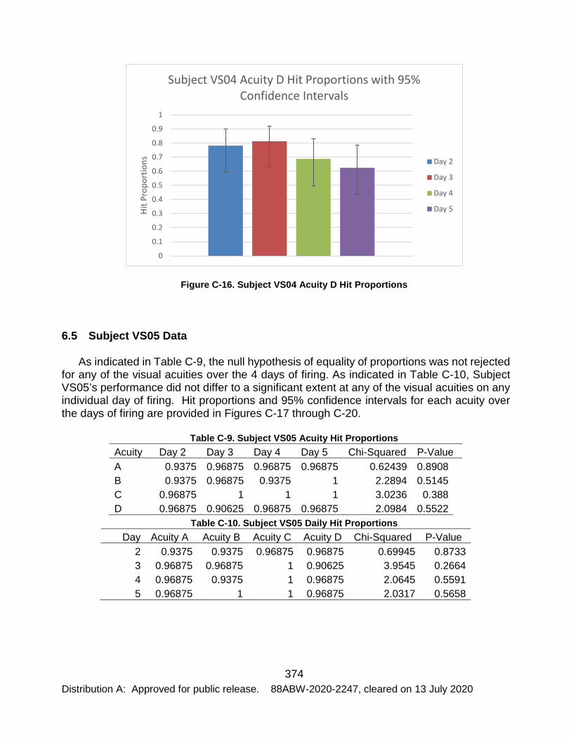
374 Distribution A: Approved for public release. 88ABW-2020-2247, cleared on 13 July 2020
Figure C-16. Subject VS04 Acuity D Hit Proportions
6.5 Subject VS05 Data
As indicated in Table C-9, the null hypothesis of equality of proportions was not rejected for any of the visual acuities over the 4 days of firing. As indicated in Table C-10, Subject VS05’s performance did not differ to a significant extent at any of the visual acuities on any individual day of firing. Hit proportions and 95% confidence intervals for each acuity over the days of firing are provided in Figures C-17 through C-20.
Table C-9. Subject VS05 Acuity Hit Proportions Acuity Day 2 Day 3 Day 4 Day 5 Chi-Squared P-Value A 0.9375 0.96875 0.96875 0.96875 0.62439 0.8908 B 0.9375 0.96875 0.9375 1 2.2894 0.5145 C 0.96875 1 1 1 3.0236 0.388 D 0.96875 0.90625 0.96875 0.96875 2.0984 0.5522
Table C-10. Subject VS05 Daily Hit Proportions Day Acuity A Acuity B Acuity C Acuity D Chi-Squared P-Value
2 0.9375 0.9375 0.96875 0.96875 0.69945 0.8733 3 0.96875 0.96875 1 0.90625 3.9545 0.2664 4 0.96875 0.9375 1 0.96875 2.0645 0.5591 5 0.96875 1 1 0.96875 2.0317 0.5658
0
0.1
0.2
0.3
0.4
0.5
0.6
0.7
0.8
0.9
1
Hit P
ropo
rtio
ns
Subject VS04 Acuity D Hit Proportions with 95% Confidence Intervals
Day 2
Day 3
Day 4
Day 5

375 Distribution A: Approved for public release. 88ABW-2020-2247, cleared on 13 July 2020
Figure C-17. Subject VS05 Acuity A Hit Proportions
Figure C-18. Subject VS05 Acuity B Hit Proportions
0
0.2
0.4
0.6
0.8
1
1.2
Hit P
ropo
rtio
ns
Subject VS05 Acuity A Hit Proportions with 95% Confidence Intervals
Day 2
Day 3
Day 4
Day 5
0
0.2
0.4
0.6
0.8
1
1.2
Hit P
ropo
rtio
ns
Subject VS05 Acuity B Hit Proportions with 95% Confidence Intervals
Day 2
Day 3
Day 4
Day 5

376 Distribution A: Approved for public release. 88ABW-2020-2247, cleared on 13 July 2020
Figure C-19. Subject VS05 Acuity C Hit Proportions
Figure C-20. Subject VS05 Acuity D Hit Proportions
6.6 Subject VS06 Data
As indicated in Table C-11, the null hypothesis of equality of proportions was not rejected
0
0.2
0.4
0.6
0.8
1
1.2
Hit P
ropo
rtio
ns
Subject VS05 Acuity C Hit Proportions with 95% Confidence Intervals
Day 2
Day 3
Day 4
Day 5
0
0.2
0.4
0.6
0.8
1
1.2
Hit P
ropo
rtio
ns
Subject VS05 Acuity D Hit Proportions with 95% Confidence Intervals
Day 2
Day 3
Day 4
Day 5

377 Distribution A: Approved for public release. 88ABW-2020-2247, cleared on 13 July 2020
for any of the visual acuities over the 4 days of firing. As indicated in Table C-12, Subject VS06’s performance did not differ to a significant extent at any of the visual acuities on any individual day of firing. Hit proportions and 95% confidence intervals for each acuity over the days of firing are provided in Figures C-21 through C-24.
Table C-11. Subject VS06 Acuity Hit Proportions Acuity Day 2 Day 3 Day 4 Day 5 Chi-Squared P-Value A 1 1 1 1 NA NA B 1 1 1 1 NA NA C 1 1 1 1 NA NA D 0.96875 1 1 1 3.0236 0.388
Table C-12. Subject VS06 Daily Hit Proportions Day Acuity A Acuity B Acuity C Acuity D Chi-Squared P-Value
2 1 1 1 0.96875 2.8984 0.4076 3 1 1 1 1 NA NA 4 1 1 1 1 NA NA 5 1 1 1 1 NA NA
Figure C-21. Subject VS06 Acuity A Hit Proportions
0.75
0.8
0.85
0.9
0.95
1
1.05
Hit P
ropo
rtio
ns
Subject VS06 Acuity A Hit Proportions with 95% Confidence Intervals
Day 2
Day 3
Day 4
Day 5

378 Distribution A: Approved for public release. 88ABW-2020-2247, cleared on 13 July 2020
Figure C-22. Subject VS06 Acuity B Hit Proportions
Figure C-23. Subject VS06 Acuity C Hit Proportions
0.75
0.8
0.85
0.9
0.95
1
1.05
Hit P
ropo
rtio
ns
Subject VS06 Acuity B Hit Proportions with 95% Confidence Intervals
Day 2
Day 3
Day 4
Day 5
0.75
0.8
0.85
0.9
0.95
1
1.05
Hit P
ropo
rtio
ns
Subject VS06 Acuity C Hit Proportions with 95% Confidence Intervals
Day 2
Day 3
Day 4
Day 5

379 Distribution A: Approved for public release. 88ABW-2020-2247, cleared on 13 July 2020
Figure C-24. Subject VS06 Acuity D Hit Proportions
6.7 Subject VS07 Data
As indicated in Table C-13, the null hypothesis of equality of proportions was not rejected for any of the visual acuities over the 4 days of firing. As indicated in Table C-14, Subject VS07’s performed did not differ to a significant extent at any of the visual acuities on any individual day of firing. Hit proportions and 95% confidence intervals for each acuity over the days of firing are provided in Figures C-25 through C-28.
Table C-13. Subject VS07 Acuity Hit Proportions Acuity Day 2 Day 3 Day 4 Day 5 Chi-Squared P-Value A 1 0.96875 0.96875 1 2.0317 0.5658 B 0.96875 1 1 1 30.236 0.388 C 1 1 1 1 NA NA D 1 1 1 1 NA NA
Table C-14. Subject VS07 Daily Hit Proportions Day Acuity A Acuity B Acuity C Acuity D Chi-Squared P-Value
2 1 0.96876 1 1 3.0236 0.388 3 0.96875 1 1 1 2.9923 0.3928 4 0.96875 1 1 1 3.0236 0.388 5 1 1 1 1 NA NA
0
0.2
0.4
0.6
0.8
1
1.2
Hit P
ropo
rtio
ns
Subject VS06 Acuity D Hit Proportions with 95% Confidence Intervals
Day 2
Day 3
Day 4
Day 5
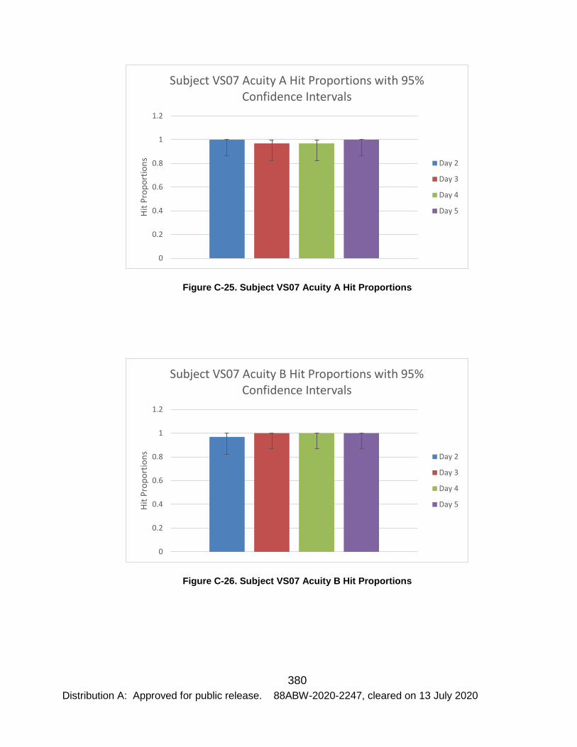
380 Distribution A: Approved for public release. 88ABW-2020-2247, cleared on 13 July 2020
Figure C-25. Subject VS07 Acuity A Hit Proportions
Figure C-26. Subject VS07 Acuity B Hit Proportions
0
0.2
0.4
0.6
0.8
1
1.2
Hit P
ropo
rtio
ns
Subject VS07 Acuity A Hit Proportions with 95% Confidence Intervals
Day 2
Day 3
Day 4
Day 5
0
0.2
0.4
0.6
0.8
1
1.2
Hit P
ropo
rtio
ns
Subject VS07 Acuity B Hit Proportions with 95% Confidence Intervals
Day 2
Day 3
Day 4
Day 5

381 Distribution A: Approved for public release. 88ABW-2020-2247, cleared on 13 July 2020
Figure C-27. Subject VS07 Acuity C Hit Proportions
Figure C-28. Subject VS07 Acuity D Hit Proportions
6.8 Subject VS08 Data
As indicated in Table C-15, the null hypothesis of equality of proportions was rejected
0.75
0.8
0.85
0.9
0.95
1
1.05
Hit P
ropo
rtio
ns
Subject VS07 Acuity C Hit Proportions with 95% Confidence Intervals
Day 2
Day 3
Day 4
Day 5
0.75
0.8
0.85
0.9
0.95
1
1.05
Hit P
ropo
rtio
ns
Subject VS07 Acuity D Hit Proportions with 95% Confidence Intervals
Day 2
Day 3
Day 4
Day 5

382 Distribution A: Approved for public release. 88ABW-2020-2247, cleared on 13 July 2020
for visual acuity B on day 2 of firing. As indicated in Table C-16, Subject VS08’s performance at acuity C was significantly lower than the other acuities on day 3 of firing. Hit proportions and 95% confidence intervals for each acuity over the days of firing are provided in Figures C-29 through C-32.
Table C-15. Subject VS08 Acuity Hit Proportions Acuity Day 2 Day 3 Day 4 Day 5 Chi-Squared P-Value A 1 1 1 1 NA NA B 0.90625 1 1 1 9.216 0.02655 C 0.96875 0.90625 0.90625 0.96875 2.1333 0.5452 D 0.9375 1 0.96875 0.9375 2.2894 0.5145
Table C-16. Subject VS08 Daily Hit Proportions Day Acuity A Acuity B Acuity C Acuity D Chi-Squared P-Value
2 1 0.90625 0.96875 0.9375 3.4973 0.3211 3 1 1 0.90625 1 9.216 0.02655 4 1 1 0.90625 0.96875 6.1935 0.1026 5 1 1 0.96875 0.9375 3.7547 0.2892
Figure C-29. Subject VS08 Acuity A Hit Proportions
0.75
0.8
0.85
0.9
0.95
1
1.05
Hit P
ropo
rtio
ns
Subject VS08 Acuity A Hit Proportions with 95% Confidence Intervals
Day 2
Day 3
Day 4
Day 5

383 Distribution A: Approved for public release. 88ABW-2020-2247, cleared on 13 July 2020
Figure C-30. Subject VS08 Acuity B Hit Proportions
Figure C-31. Subject VS08 Acuity C Hit Proportions
0
0.2
0.4
0.6
0.8
1
1.2
Hit P
ropo
rtio
ns
Subject VS08 Acuity B Hit Proportions with 95% Confidence Intervals
Day 2
Day 3
Day 4
Day 5
0
0.2
0.4
0.6
0.8
1
1.2
Hit P
ropo
rtio
ns
Subject VS08 Acuity C Hit Proportions with 95% Confidence Intervals
Day 2
Day 3
Day 4
Day 5

384 Distribution A: Approved for public release. 88ABW-2020-2247, cleared on 13 July 2020
Figure C-32. Subject VS08 Acuity D Hit Proportions
6.9 Subject VS09 Data
As indicated in Table C-17, the null hypothesis of equality of proportions was not rejected for any of the visual acuities over the 4 days of firing. As indicated in Table C-18, Subject VS09’s performance did not differ to a significant extent at any of the visual acuities on any individual day of firing. Hit proportions and 95% confidence intervals for each acuity over the days of firing are provided in Figures C-33 through C-36.
Table C-17. Subject VS09 Acuity Hit Proportions Acuity Day 2 Day 3 Day 4 Day 5 Chi-Squared P-Value A 0.96875 1 1 0.96875 2.0317 0.5658 B 1 1 1 1 NA NA C 0.9375 1 0.96875 0.96875 2.0645 0.5591 D 1 0.96875 0.90625 1 6.1935 0.1026
Table C-18. Subject VS09 Daily Hit Proportions Day Acuity A Acuity B Acuity C Acuity D Chi-Squared P-Value
2 0.96875 1 0.9375 1 3.7547 0.2892 3 1 1 1 0.96875 3.0236 0.388 4 1 1 0.96875 0.90624 6.1935 0.1026 5 0.96875 1 0.96875 1 2.0317 0.5658
0
0.2
0.4
0.6
0.8
1
1.2
Hit P
ropo
rtio
ns
Subject VS08 Acuity D Hit Proportions with 95% Confidence Intervals
Day 2
Day 3
Day 4
Day 5

385 Distribution A: Approved for public release. 88ABW-2020-2247, cleared on 13 July 2020
Figure C-33. Subject VS09 Acuity A Hit Proportions
Figure C-34. Subject VS09 Acuity B Hit Proportions
0
0.2
0.4
0.6
0.8
1
1.2
Hit P
ropo
rtio
ns
Subject VS09 Acuity A Hit Proportions with 95% Confidence Intervals
Day 2
Day 3
Day 4
Day 5
0.75
0.8
0.85
0.9
0.95
1
1.05
Hit P
ropo
rtio
ns
Subject VS09 Acuity B Hit Proportions with 95% Confidence Intervals
Day 2
Day 3
Day 4
Day 5

386 Distribution A: Approved for public release. 88ABW-2020-2247, cleared on 13 July 2020
Figure C-35. Subject VS09 Acuity C Hit Proportions
Figure C-36. Subject VS09 Acuity D Hit Proportions
6.10 Subject VS10 Data
As indicated in Table C-19, the null hypothesis of equality of proportions was not rejected
0
0.2
0.4
0.6
0.8
1
1.2
Hit P
ropo
rtio
ns
Subject VS09 Acuity C Hit Proportions with 95% Confidence Intervals
Day 2
Day 3
Day 4
Day 5
0
0.2
0.4
0.6
0.8
1
1.2
Hit P
ropo
rtio
ns
Subject VS09 Acuity D Hit Proportions with 95% Confidence Intervals
Day 2
Day 3
Day 4
Day 5

387 Distribution A: Approved for public release. 88ABW-2020-2247, cleared on 13 July 2020
for any of the visual acuities over the 4 days of firing. While the null hypothesis was not rejected for acuity D, Table C-19 does provide evidence that indicates that Subject VS10 does appear to have had difficulty at acuity D, and that this difficulty was more pronounced on days 2 and 3 of firing. As indicated in Table C-20, Subject VS10’s performance at acuity D on day 3 was significantly lower than performance at the other acuities. Hit proportions and 95% confidence intervals for each acuity over the days of firing are provided in Figures C-37 through C-40.
Table C-19. Subject VS10 Acuity Hit Proportions Acuity Day 2 Day 3 Day 4 Day 5 Chi-Squared P-Value A 0.90625 0.9375 1 1 5.6195 0.1317 B 0.96875 1 1 1 3.0236 0.388 C 0.84375 0.96875 0.9375 0.96875 5.1391 0.1619 D 0.71875 0.78125 0.90625 0.90625 5.928 0.1152
Table C-20. Subject VS10 Daily Hit Proportions Day Acuity A Acuity B Acuity C Acuity D Chi-Squared P-Value
2 0.90625 0.96875 0.84375 0.71875 9.0505 0.02863 3 0.9375 1 0.96875 0.78125 12.583 0.005631 4 1 1 0.9375 0.90625 5.6195 0.1317 5 1 1 0.96875 0.90625 6.1935 0.1026
Figure C-37. Subject VS10 Acuity A Hit Proportions
0
0.2
0.4
0.6
0.8
1
1.2
Hit P
ropo
rtio
ns
Subject VS10 Acuity A Hit Proportions with 95% Confidence Intervals
Day 2
Day 3
Day 4
Day 5

388 Distribution A: Approved for public release. 88ABW-2020-2247, cleared on 13 July 2020
Figure C-38. Subject VS10 Acuity B Hit Proportions
Figure C-39. Subject VS10 Acuity C Hit Proportions
0
0.2
0.4
0.6
0.8
1
1.2
Hit P
ropo
rtio
ns
Subject VS10 Acuity B Hit Proportions with 95% Confidence Intervals
Day 2
Day 3
Day 4
Day 5
0
0.2
0.4
0.6
0.8
1
1.2
Hit P
ropo
rtio
ns
Subject VS10 Acuity C Hit Proportions with 95% Confidence Intervals
Day 2
Day 3
Day 4
Day 5
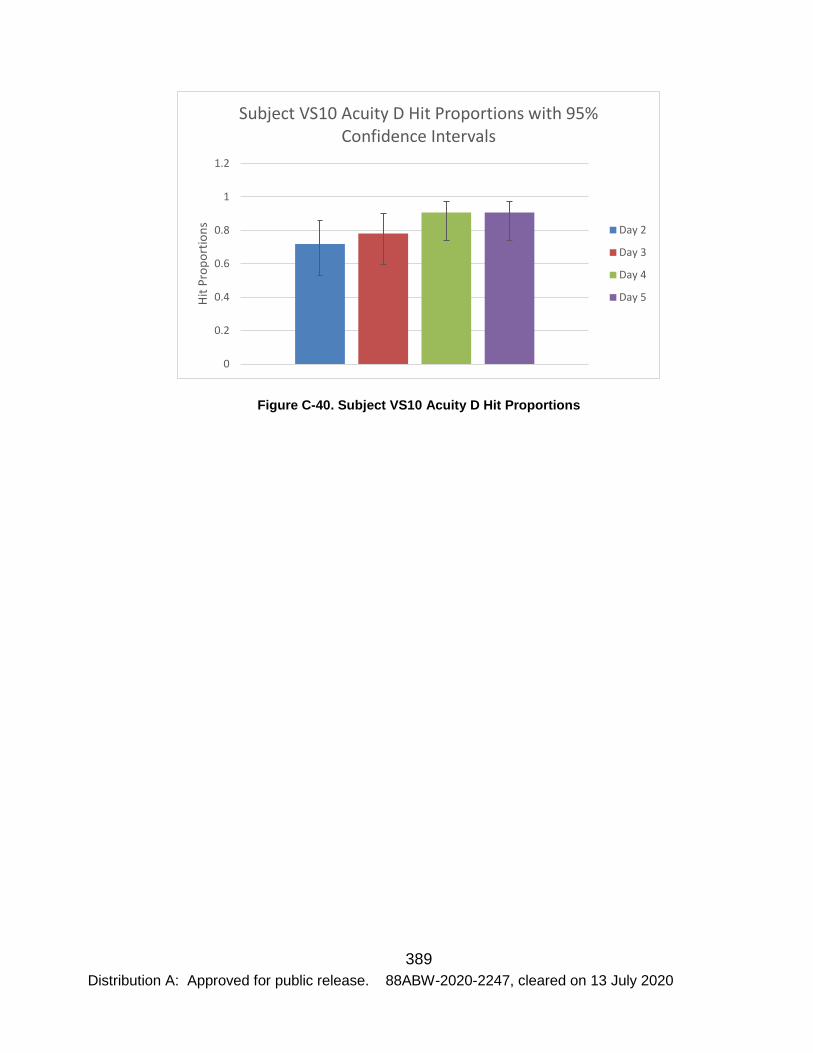
389 Distribution A: Approved for public release. 88ABW-2020-2247, cleared on 13 July 2020
Figure C-40. Subject VS10 Acuity D Hit Proportions
0
0.2
0.4
0.6
0.8
1
1.2
Hit P
ropo
rtio
ns
Subject VS10 Acuity D Hit Proportions with 95% Confidence Intervals
Day 2
Day 3
Day 4
Day 5