Market Externalities of Large Unemployment

Insurance Extension Programs∗

Rafael Lalive†

University of Lausanne

Camille Landais‡

London School of Economics

Josef Zweimuller§

University of Zurich.

July 29, 2015

Abstract

We provide evidence that unemployment insurance affects equilibrium conditions

in the labor market, which creates significant “market externalities. We provide a

framework for identification of such equilibrium effects and implement it using the

Regional Extension Benefit Program in Austria which extended the duration of UI

benefits for a large group of eligible workers in selected regions of Austria. We

show that non-eligible workers in REBP regions have higher job finding rates, lower

unemployment durations, and a lower risk of long-term unemployment. We discuss

the implications of our results for optimal UI policy.

JEL Classification: J64, H23

Keywords: Unemployment insurance

∗We would like to thank Josh Angrist, Henrik Kleven, Pascal Michaillat, Johannes Spinnewijn, Em-manuel Saez, Andrea Weber, Rudolf Winter-Ebmer, four anonymous referees as well as seminar audiencesat Columbia University, UC Davis, Northwestern University, Harvard University, NBER, London Schoolof Economics, Paris School of Economics, CIREQ workshop in Montreal, Uppsala, CAGE/Warwick 2014workshop in Venice, Bergen-Stavanger 2014 workshop at NHH Bergen, CREST-INSEE, PUC-Rio, PEUKWarwick, Bristol, University of British Columbia, CEMFI, the 2014 Bruchi Luchino workshop and theEuropean Summer Symposium in Labor Economics (ESSLE) for very helpful comments. Philippe Ruhprovided excellent research assistance. We are particularly grateful to Manfred Zauner for his support inacquiring the vacancy data. Rafael Lalive acknowledges financial support by the Swiss National Centerof Competence in Research LIVES. Josef Zweimuller acknowledges funding from the Austrian NationalScience Research Network Labor Market and Welfare State of the Austrian FWF. The authors declarethat they have no relevant or material financial interests that relate to the research described in thispaper†Department of Economics, University of Lausanne, CH-1015 Lausanne-Dorigny,

Rafael.Lalive@unil.ch. R.Lalive is also associated with CEPR, CESifo, IFAU, IZA, IfW and Uni-versity of Zurich.‡Dept of Economics, Houghton Street London, WC2A 2AE +44(0)20-7955-7864, c.landais@lse.ac.uk§Department of Economics, Schonberggasse 1, CH-8001 Zurich; josef.zweimueller@econ.uzh.ch.

J.Zweimuller is also associated with CEPR, CESifo and IZA

The probability that an unemployed individual finds a job depends on her job search

strategy and on labor market conditions determining how easy (or difficult) it is to be

matched to a potential employer.1 Changes in unemployment insurance (UI) policies

affect the search strategy of unemployed workers which in turn affects their job search

outcomes. This is the micro effect of UI. Changes in UI policies also affect equilibrium

labor market conditions which in turn will affect the job finding probability for any given

search strategy. We call this second effect market externalities of UI.

The micro effect can be identified by comparing two individuals with different levels of

UI generosity in the same labor market. A large number of well-identified estimates of the

micro effect have shown that more generous UI benefits tend to increase unemployment

duration.2 In contrast, evidence on market externalities is scarce. The aim of this paper

is to bridge this gap.

Market externalities of UI are important for at least two reasons. First, the overall

effect of variations in UI on search outcomes, the macro effect, consists of both the micro

effect and market externalities. Studies comparing individuals subject to differential UI

benefit generosity within the same labor market identify the micro effect. These studies

cannot shed light on the true effect of UI if externalities are important. Second, market

externalities have first order welfare effects, as shown in Landais, Michaillat and Saez

[2010]. This implies that the sign and magnitude of market externalities is critical to

determine the optimal level of UI.

There is no theoretical consensus on the sign and magnitude of market externalities

of UI. And it is empirically challenging to estimate market externalities because general

equilibrium effects are typically hard to identify. Recent papers have tried to directly

estimate equilibrium effects of active labor market policies such as randomized programs

of counselling for job seekers without reaching a clear consensus (Blundell et al. [2004],

Ferracci, Jolivet and van den Berg [2010], Gautier et al. [2012]).3 More recently, Crepon

et al. [2013] analyze a job search assistance program for young educated unemployed in

France with two levels of randomization: the share of treated was randomly assigned across

labor markets, and within each labor market individual treatment was also randomized.

1Setting a job search strategy involves decisions such as: how hard to search, what jobs to search for,how to set one’s reservation wage, etc. Labor market conditions depend on the number of job searchers(and the intensity with which they search), on the number of available jobs, and on the extent to whichlabor market frictions inhibit immediate matching of job searchers to open vacancies.

2See for instance Krueger and Meyer [2002] for a survey of early studies. More recent studies includeLandais [2013] for the US, Schmieder, von Wachter and Bender [2012b] for Germany or Lalive andZweimuller [2004a,b] for Austria.

3Blundell et al. [2004] study the effect of a counselling program for young unemployed in the UK andfind little evidence of displacement effects. Ferracci, Jolivet and van den Berg [2010] study a programfor young employed workers in France and find that the direct effect of the program is smaller in labormarkets where a larger fraction of the labor force is treated. Gautier et al. [2012] analyze a randomizedjob search assistance program organized in 2005 in two Danish counties. Comparing control individualsin experimental counties to job seekers in some similar non-participating counties, their results suggestthe presence of substantial negative spillovers.

1

They find evidence of significant displacement effects for unemployed men who were not

in the program. But take-up of the training program was low (35%) and many job seekers

were already employed at the time of the experiment, substantially limiting the statistical

power to detect displacement effects.

Contrary to UI, active labor market programs do not directly affect outside options

of workers in the wage bargaining process, and miss a potentially important element

of equilibrium adjustments through wages. Active labor market programs are therefore

only partially informative about the market externalities of UI. We are aware of only one

paper that studies market externalities of UI. Levine [1993] finds that increases in the

replacement rate of UI decreases unemployment duration among the unemployed who are

ineligible for UI. Hagedorn et al. [2013] estimate a macro elasticity of unemployment with

respect to UI variations for the U.S. by comparing counties on the border of states with

different potential benefit duration. Our estimates are compatible with the macro elas-

ticity they find. Our results complement their findings in suggesting that the micro effect

is larger than the macro effect, due to the existence of significant market externalities.

In this paper we shed new light on market externalities of UI. First, we show how

market externalities can be identified in a quasi-experimental setting by looking at the

effect of a UI benefit variation in a given labor market on job search outcomes of workers

who are not eligible to the UI benefit variation but who search in the same labor market.

We define the relevant labor market as the place where workers are competing for the same

vacancies, and propose a new method to determine the scope of a labor market using

vacancy data. Second, we implement this strategy and offer evidence of the existence

of market externalities of UI benefit extensions using the Regional Extension Benefit

Program (REBP) in Austria. This program extended unemployment benefits drastically

for a large subset of workers in selected regions of Austria from June 1988 until August

1993. We focus on unemployed workers in REBP regions who are similar to the eligible

unemployed, compete for the same vacancies, but are not eligible for REBP because they

fail to meet the eligibility requirements of the REBP program. Using a difference-in-

difference identification strategy, we compare these non-eligible unemployed to similar

non-eligible unemployed in non-REBP regions to identify the effect of REBP on duration

of job search of non-eligible unemployed in treated markets.

The REBP is a compelling empirical setting to study market externalities of UI. First,

treated workers received an extra three years of covered unemployment with an unchanged

benefit level. This large UI extension generated a strong increase in unemployment dura-

tion of treated workers thereby manipulating equilibrium labor market conditions [Lalive,

2008]. Second, REBP was enacted only in a subset of regions (28 of about 100 regions)

and, within treated regions, 90% of workers above 50 years old were eligible to the pro-

gram. This allows us to study how ineligible job seekers in REBP regions compare to

similar workers in non-REBP regions. While the choice of treated regions and workers

2

is partially endogenous, we use specific features of the REBP program to build a credi-

ble identification strategy. Finally, administrative data on the universe of unemployment

spells is available in Austria since the 1980s. By matching data from the unemployment

register with social security data on the universe of employment spells in Austria since

1949, we can determine eligibility status for the REBP program along all eligibility dimen-

sions. Our data also enable us to look at many different outcomes, from unemployment

and non-employment durations, to reemployment characteristics and wages. As the data

cover sufficiently long periods before and after the REBP program, we are able to study

whether externalities appear during the program and whether they disappear after the

program is repealed.

Our results demonstrate the presence of sizable market externalities of UI. REBP

induced a 2 to 4 weeks decrease in the average unemployment duration of all non-eligible

workers aged 46 to 54 compared to similar workers from non REBP regions. For non-

eligible workers aged 50 to 54, who are competing for similar vacancies as treated workers,

unemployment duration decreases by 6 to 8 weeks. These effects are the largest when the

program intensity reaches its highest level, then decrease and disappear as the program

is scaled down and finally interrupted. In our robustness analysis, we address the two

main potential confounders for our results. First, we provide evidence that our results are

unlikely to be driven by region-specific shocks contemporaneous with the REBP program.

Second, we show that our results are unlikely to be confounded by selection, i.e. a change

in unobserved characteristics of non-eligible workers contemporaneous with the REBP

program. We also show evidence that the magnitude of the externalities on non-eligible

workers increases with the intensity of the REBP treatment across local labor markets.

We finally identify the presence of geographical spillovers of the REBP program on non-

REBP regions that have labor markets that are highly integrated to REBP regions.

Our empirical findings have important policy implications. First, the presence of sig-

nificant market externalities implies that the micro and the macro effect of UI extensions

will differ. Our estimates imply a significant wedge between the micro (em) and the macro

(eM) effect of UI extensions on the job finding rate of workers in labor markets that were

treated by REBP: W = 1 − eM/em ≈ .21. In the REBP setting, a segment only of the

labor force was treated, and substitution opportunities to treated workers were potentially

available in non-treated labor markets. We show that our estimated wedge is therefore

a lower bound on the magnitude of the wedge when the whole labor force is treated by

a change in UI benefits. Second, our results bear important implications for the design

of optimal UI policies. Our results imply that more generous UI benefits increase labor

market tightness and the job finding rate per unit of search effort. As a consequence,

the optimal level of UI will be larger than suggested by the partial equilibrium Baily-

Chetty formula (Chetty [2006]), as explained in Landais, Michaillat and Saez [2010]. This

means that temporary extensions enacted in reaction to business cycles downturns are

3

less socially costly than what a partial equilibrium representation would suggest.

The remainder of the paper is organized as follows. Section I presents our theoretical

framework, explains the concept of market externalities and how they can be identi-

fied. Section II presents the institutional background of the REBP program. Section

III presents the data and our empirical strategy. It also shows how we can use vacancy

data to identify groups of non-treated workers competing with treated workers for jobs

in the same labor market. Section IV presents the results as well as our robustness and

heterogeneity analysis. Section V draws welfare and policy implications.

I Market externalities of UI and their identification

The probability that an individual finds a job depends on how hard that individual

searches for a job and/or on how selective she is in her acceptance decisions. It also

depends on the labor market conditions that determine how easy it is to locate jobs or to

be matched to a potential employer. These two forces are usually represented in equilib-

rium search and matching models by the stylized decomposition: hi = ei · f(θ). h is the

hazard rate out of unemployment. ei captures the search effort / selectiveness component.

θ is the ratio of job vacancies to total search effort, and represents the tightness of the

labor market. f(θ) therefore captures the effect of labor market conditions on the job

finding probability per unit of effort.4 If there are no job vacancies created by employers,

then f(θ) = 0 and no amount of search effort by an unemployed worker would yield a

positive probability of obtaining a job.

Changes in unemployment benefit policies affect the search intensity and selectiveness

of unemployed workers. We call this effect the micro effect of UI. It can be identified by

comparing two individuals with different levels of UI generosity in the same labor market.

However, changes in UI generosity also affect labor market conditions and the job finding

rate per unit of search effort. We call this second effect market externalities. It stems

from equilibrium adjustments in labor market tightness θ in response to a change in UI

generosity. The overall effect on the job finding rate of a change in UI, the macro effect

of UI, is therefore the sum of the micro effect and market externalities.

There are at least two reasons why we care about identifying the presence of market

externalities of UI. First, when the generosity of UI varies, for instance due to UI benefit

extensions such as the recent EUC program in the US, the total effect on unemployment

will be the sum of the micro effect and of market externalities. Studies comparing in-

dividuals with different UI benefits within the same labor market will typically identify

only the micro effect, and cannot shed light on the true effect of such UI extensions.

Second, as shown in Landais, Michaillat and Saez [2010], market externalities have first

4Note that f, f ′ > 0, f ′′ < 0 characterizes the matching process in a labor market with frictions.

4

order welfare effects whenever the Hosios condition is not met. The sign and magnitude

of market externalities is therefore critical to determine the optimal level of UI.

As explained in Landais, Michaillat and Saez [2010], using the framework developed by

Michaillat [2012], the sign and magnitude of market externalities depends on two forces:

the rat race effect and the wage effect. Appendix A gives a detailed theoretical presenta-

tion of the framework, derives the formula for market externalities and the decomposition

into the rat race effect and the wage effect.

The rat race effect arises when labor demand is not perfectly elastic and does not fully

adjust to variations in search effort of unemployed workers, which will be the case when

technology exhibits diminishing returns to labor.5 Intuitively, in the extreme case when

there is a fixed number of jobs, an increase in an individual’s search effort will increase her

probability of finding a job. However, this must come at the expense of the probability

of all other unemployed to find a job as the total number of jobs remains unchanged.

Hence an increase in UI generosity, by decreasing aggregate search effort, increases the

probability of finding a job per unit of search effort f(θ). The rat race effect creates a

positive market externality.

The wage effect arises when wages are determined through a bargaining process. An

increase in UI generosity improves workers’ outside option and tend to increase wages.

This decreases the return from opening vacancies for firms, leading to a decrease in labor

demand. Thus the wage effect creates a negative market externality.

The overall effect of a change in UI benefits on equilibrium labor market tightness will

therefore depend on the relative magnitude of these two effects. When wages do not react

to a particular policy, the rat race effect will be the only driver of labor market tightness

adjustments to the policy. Studies estimating spillover effects of active labor market or

training programs such as Crepon et al. [2013] therefore tend to capture a pure rat race

effect as these training programs are unlikely to affect bargained wages.

To identify market externalities, our strategy compares two groups of workers who are

searching for jobs in the same labor market. The first group is “treated” and experiences

an exogenous change of UI generosity, while the second group is not treated and does

not experience any change in UI benefits. The individual search effort of treated workers

will respond, changing their job finding probability. This change in search effort will also

affect equilibrium labor market tightness and therefore the job finding probability per

unit of search effort, creating labor market externalities. The change in the job finding

probability of non-treated workers will capture these market externalities.

In appendix A.2, we show under which conditions a change in the job finding probabil-

ity of non-treated workers can identify labor market externalities. The key identification

5Diminishing returns is a sufficient but not a necessary condition for the presence of a downwardsloping labor demand. Landais, Michaillat and Saez [2010] show for instance that an “aggregate demandmodel” with a quantity equation for money and nominal wage rigidities will feature a downward slopinglabor demand even with linear technology.

5

requirement is that treated and non-treated workers are in the same labor market, where a

labor market is defined as the market place where workers compete for the same vacancies.

From a search-theoretic standpoint, this definition is the most natural: it follows from

the law of one price, which defines one equilibrium labor market tightness for each labor

market. In practice this means that each labor market is characterized by a vacancy type,

and matching between the workers competing for these vacancies and employers posting

these vacancies exhibits randomness. In other words, when treated and non-treated work-

ers compete for these vacancies, a firm opening one such vacancy cannot know whether

it will be matched to a treated or to a non-treated worker. When this is the case, we

show in appendix A.2 that variations in the job finding probability of non-treated workers

in response to a change of UI for treated workers will identify market externalities of UI

and that, as the size of the treated group compared to the non-treated group increases,

market externalities on non-treated workers converge to identifying the equilibrium ef-

fects of treating the whole market. Importantly, market externalities identified through

the change in the job finding probability of non-treated workers will capture the wage

effect even if wages are bargained at the individual level. The intuition is that within a

labor market, because of random matching, the expected profit of opening vacancies is

the weighted average of the profits of opening vacancies for each group of workers. There-

fore the increase in bargained wages of treated workers will reduce the expected profit of

opening vacancies and will then affect overall vacancy posting in the market.

In appendix A.3, we also discuss the case when treated and non-treated workers do

not compete for the same vacancies, for instance because firms can discriminate between

treated and non-treated workers by offering them different types of vacancies. In that case,

non-treated workers will not be in the same labor market as treated workers and changes in

the job finding probability of non-treated workers will no longer directly identify variations

in labor market tightness for the treated labor market. Yet, UI variations for treated

workers may nevertheless still create externalities for non-treated workers. As shown

in appendix A.3, such externalities will arise across labor markets due to substitution

effects and are different in nature and magnitude from market externalities within a labor

market. The existence of externalities across labor markets due to substitution effects

bears implications for the interpretation of our results that we discuss in section V.

Identification of market externalities of UI extensions within a labor market requires

the ability to find two groups of workers with different UI levels within the same labor

market, i.e. competing for similar vacancies. Using vacancy data, we propose below a

simple method to determine whether two groups of workers are competing for similar job

vacancies by looking at how characteristics of job vacancies predict the group affiliation

of the individual filling the vacancy.

6

II Austrian Unemployment Insurance and the REBP

Unemployment Insurance and Wage Setting Systems The Austrian UI system

is more restrictive than many other continental European systems and closer to the U.S.

system in terms of generosity. Workers who become unemployed can draw regular un-

employment benefits (UB), the amount of which depends on previous earnings. In 1990,

the replacement ratio (UB relative to gross monthly earnings) was 40.4 % for the median

income earner; 48.2 % for a worker earning half the median; and 29.6 % for a worker

earning twice the median. UB payments are not taxed, not means-tested, and there is no

experience rating.

The maximum number of weeks that one can receive UB (potential duration) depends

on work history (the number of weeks worked prior to becoming unemployed) and age.

For the age group 50 and older, UB-duration is 52 weeks; and for the age group 40-49, UB-

duration is 39 weeks. Voluntary quitters and workers laid off for misconduct can receive

UB but are subject to a waiting period of 4 weeks. UB recipients need to search actively

for a new job within the scope of the claimant’s qualifications. After UB payments have

been exhausted, job seekers can apply for post-UB transfers (“Notstandshilfe”). These

transfers are means-tested and depend on income and wealth of other family members

and close relatives. They are granted for successive 39-week periods after which eligibility

requirements are recurrently checked and can last for an indefinite time period. Post-UB

transfers can be at most 92 % of UB. In 1990, the median post-UB transfer payment

was about 70 % of the median UB. The majority of the unemployed (59 %) received UB

whereas 26 % received post-UB transfers.

Another relevant feature of the Austrian labor market is its system of wage formation.

Almost all workers are covered by collective agreements which take place at the sectoral

(or the occupational) level. Collective agreements impose a lower bound on workers’

wages. While the Austrian wage setting process is more centralized than in the US and

many European countries (except for Scandinavia), wages are less rigid than one might

prima facie think. First, while Austrian wage setting institutions impose a lot of downward

rigidity on wages in ongoing employment relationships, wage adjustments take place when

workers change jobs or start a new job after an unemployment spell. Second, existing

evidence suggests that a substantial fraction of workers are paid above the collectively

agreed minimum wage.6 To the extent that older workers are more experienced and

achieve higher wages than the collectively agreed wages, the wage floors of collective

agreements are unlikely to contaminate our analysis.

6Leoni and Pollan [2011] study “overpayments” (the ratio of effective wages over collectively bargainedwages). They find that, in the years when the REBP was in place, effective wages of blue collar workerswere, on average, between 20 to 25 percent above the collectively bargained minimum wages. Hence alarge fraction of workers is paid above the wage floor.

7

Restructuring of the Austrian steel industry and the REBP After World War

II, Austria nationalized large parts of its heavy industries (iron, steel, etc). Firms in the

steel sector were part of a large holding company owned by the state, the Oesterreichische

Industrie AG, OeIAG. In 1986, after the steel industry was hit by an oil speculation

scandal and failure of a US steel-plant project, a new management was appointed and a

strict restructuring plan was implemented resulting in plant closures and downsizing.

To mitigate the labor market consequences of the restructuring plan, the Austrian

government enacted the Regional Extended Benefit Program (REBP) that extended UB-

entitlement to 209 weeks. To be eligible to 209 weeks of UB, the worker had to satisfy

each of the following criteria at the beginning of his or her unemployment spell: (i) age

50 or older; (ii) a continuous work history (780 employment weeks during the last 25

years prior to the current unemployment spell); (iii) location of residence in one of 28

selected labor market districts for at least 6 months prior to the claim; and (iv) start of

a new unemployment spell after June 1988 or spell in progress in June 1988. Note that

the REBP did not impose any industry requirement. All unemployed who met criteria

(i) to (iv) were eligible, irrespective of whether they previously worked in the steel sector

or not.

The REBP was in effect until December 1991 before a reform was implemented in

January 1992. This reform enacted two changes for new spells. First, the benefit exten-

sion was abolished in 6 of the originally 28 regions. We exclude from our analysis the

set of treated regions that were excluded after the 1991-reform. Second, the 1991-reform

tightened eligibility criteria for extended benefits: new beneficiaries had to be not only res-

idents, but also previously employed in a treated region. The program stopped accepting

new entrants in August 1, 1993. Job seekers who established eligibility to REBP before

August 1993 continued to be covered. We therefore set the end of the REBP program in

August 6, 1997 (209 weeks after August 1, 1993).

Apart from the REBP, the second measure to alleviate the problems associated with

mass redundancies in the steel sector was the so-called ’steel foundation’. Firms in the

steel sector could decide whether to join in order to provide their displaced workers with

re-training activities that were organized by the foundation. Member firms were obliged

to finance the foundation. Displaced individuals who decided to join this out-placement

center were entitled to regular unemployment benefits for a period of up to 3 years (later

4 years) regardless of age and experience. In 1988, the foundation consisted of 22 firms.

We exclude all workers employed or reemployed in the steel sector to make sure that the

workers in our sample did not have access to re-training activities provided by the steel

foundation. Notice further that no other labor market policies were put in place during

the REBP period that may confound the effect of the program. Lalive and Zweimuller

[2004b] provide an extensive discussion of the context and institutional background of the

REBP and discuss the validity of the REBP as a research design.

8

As the REBP was targeted to older workers it could also be used as a pathway to

early retirement, the main pathway being retirement via the disability insurance system.

The existence of these early retirement programs creates potential complementarities with

the REBP program that are susceptible to affect search effort and labor supply in non-

trivial ways (Inderbitzin, Staubli and Zweimuller [2013]). In order to minimize these

complementarity effects and concentrate on the effects of the REBP program alone, we

focus primarily our analysis on male workers aged 50-54 as they cannot use unemployment

benefits as a direct pathway to early retirement.

III Data and identification strategy

Data Our data set covers the universe of UI spells in Austria from 1980 to 2009. In

our baseline estimation sample, and for reasons that we explain below, we focus on all

unemployed men aged 46 to 54 at the start of a spell. For each spell, we observe the dates

of entry and exit into paid unemployment, as well as information on age at the start of

the spell, region of residence at the beginning of the spell, education, marital status, etc.

This information is merged at the individual level with the universe of social security

data in Austria (Austrian Social Security Database, ASSD), which contains information

on each employment spell as well as information for each spell in a benefit program and

information on pensions and retirement. We use complementary information on insurance

spells back until 1949 to compute work history in the past 25 years for each individual to

precisely determine a worker’s REBP eligibility status.7 We also use social security data

to compute wages before and after each unemployment spell, as well as the total duration

of non-employment after the end of an employment spell. Finally, the social security data

gives us useful information about previous and subsequent employers (such as industry,

location, etc.) for each unemployment spell.

Because of early retirement programs in Austria during our period of analysis, women

above 50 and men above 55 can go directly from REBP or from regular unemployment

benefits to early retirement programs. For these workers, it is therefore unclear whether

the effect of REBP can be interpreted as a reduction in search effort or as an extensive

margin decision to exit the labor market. Search responses to UI along the intensive mar-

gin and exits from the labor markets have potentially different implications for equilibrium

analysis. Because our focus is on search externalities arising from responses to UI along

7For more information about the ASSD, see Zweimuller et al. [2009]. The ASSD covers employmentspells from 1972 onwards. To measure worker’s experience during the last 25 years (necessary to de-termine REBP-eligibility), we used complementary data from the Austrian Ministry of Social Affairson employment spells back to 1949. (The UI administration used a similar source of information onindividual experience to determine REBP-eligibility.) As we do not observe final eligibility to REBP, ourapproach is an intent-to-treat approach. There are a few observations with an experience level belowthe REBP eligibility threshold who still received more than 52 weeks of paid UI. We get rid of these fewobviously misclassified observations in our estimation sample.

9

the intensive margin, we mainly focus on unemployed men aged below 55 because they

cannot go directly from unemployment to early retirement. In our robustness analysis,

we show that our results are robust to these sample restrictions, and that externalities

can be detected on women, and on all men aged up to 59.

To determine which workers are competing for the same vacancies as REBP eligible

workers, we use detailed micro data on job vacancies posted in public employment agencies

available for the period 1994-1998.8 This data has two important features. First, the

data records detailed information about the characteristics of the vacancy.9 Second, the

vacancy data contains the personal identifier of the person who was hired for the position.

We use the identifier to see whether the successful job seeker was eligible for REBP or

not.

Identification in an experimental setting We first discuss identification in an ex-

perimental framework and discuss below how we implement it in the actual REBP setting.

There are two labor markets, M = 0, 1. Labor market M = 1 is randomly selected to re-

ceive some exogenous treatment, i.e. an increase in the potential duration of UI benefits.

Labor market M = 0 does not receive treatment and acts as a control. In labor market

M = 1, a random subset of workers is treated (T = 1) and receives a larger potential du-

ration of UI benefits while the rest of the workers do not receive treatment (T = 0). There

are three potential outcomes yTiM (where i indexes individuals): y1i1, when being treated

in a treated labor market, y0i1, when being untreated in a treated labor market, and y0

i0

when being in a non-treated labor market. We are interested in the average externality

of the treatment on outcome yi, AE = E(y0i1 − y0

i0).

Following the treatment evaluation literature, we can relate observed outcomes to the

average externality on the non-treated in treated labor markets, AENTT :

E(y0i1|T = 0,M = 1)− E(y0

i0|T = 0,M = 0) =

AENTT︷ ︸︸ ︷

E(y0i1 − y0

i0|T = 0,M = 1)

+E(y0i0|T = 0,M = 1)− E(y0

i0|T = 0,M = 0)︸ ︷︷ ︸selection

(1)

Under double randomization (of treated labor markets and of treated individuals

within labor markets), the selection term in equation 1 is zero and AENTT can be identified

8We also have some crude vacancy data available for the period 1990-1994 that we use to computeinitial labor market tightness in appendix table 9. Unfortunately, we were not able to find or constructconsistent data throughout the period enabling us to analyze vacancy responses to the REBP.

9This includes the firm identifier of the firm posting the vacancy, the date (in month) at which thevacancy is opened and the date at which it is closed, the reason for closing the vacancy, the identifier ofthe public employment service where the vacancy is posted, the industry and job classifications of the job,details on the duration and type of the contract, the age requirement if any, the education requirementif any, the gender requirement if any, and the posted wage or range of wage if any.

10

by comparing observed outcomes for the non-treated in labor market M = 1 to observed

outcomes for workers in labor market M = 0.

In our case, REBP treatment was not allocated at random, neither across nor within

labor markets. Our empirical strategy identifies AENTT adopting a difference-in-difference

design. This design is valid if unobserved differences between non-treated workers in

markets M = 0 and M = 1 remain fixed over time. We discuss below whether this

assumption is plausible and probe it in the context of robustness analyses.

In our context, treated workers (T = 1) are workers who are eligible for REBP, based

on the three eligibility criteria: age, experience and geography. To implement our diff-

in-diff strategy, (i) we need to properly define treated labor markets M = 1 and (ii), we

also need to properly define control labor markets M = 0.

Defining treated labor markets Our analysis focuses on non-eligible workers within

REBP counties, i.e. on workers who both live and had previous employment in REBP

counties. However, to properly define treated labor markets, we want to focus on non-

eligible workers within REBP counties who actually compete for the same job vacancies as

treated workers. If treated and non-treated workers are competing for similar vacancies,

the effect of the REBP on non-treated workers can identify equilibrium variations in labor

market tightness in the labor market. If treated and non-treated workers are competing

for different vacancies, there are in practice two search markets for labor, and the effect

of the program on non-treated workers identify market externalities due to substitution

effects.

To determine which groups of workers within REBP counties are competing for the

same vacancies as REBP eligible workers, we propose a method based on micro data on

job vacancies. The vacancy data contain, for each individual vacancy, detailed information

about the characteristics of the vacancy and the personal identifier of the person who filled

the vacancy. Our strategy uses all the information on each vacancy, and estimates how

well the characteristics of each vacancy predict the REBP eligibility status of the worker

who fills the vacancy. (Data and empirical strategy are discussed in detail in appendix

B.)

To implement this strategy, we regress the probability that the worker filling a given

vacancy is eligible to REBP on a vector of all the characteristics of the vacancy and run

the model separately for various categories of non-eligible workers against eligible workers.

For each of the categories of non-eligible workers, we then analyze the predictive power

of the model using various goodness-of-fit measures.10

10This model aims at testing the ability of firms to direct their search towards different types ofworkers, who have different search effort due to REBP, by opening different types of vacancies. Wetherefore estimate it in REBP regions when the REBP was in place. In places or times where REBP isnot in place, workers eligible to REBP (would the REBP be in place) and non-eligible workers have thesame level of UI benefits, their search effort is likely to be very similar, and firms have therefore much

11

In figure 1 panel A, we plot the p-value of two standard goodness-of-fit tests for the logit

model, the Pearson’s χ2 goodness-of-fit test and the Hosmer-Lemeshow χ2 goodness-of-fit

test, for different categories of non-eligible workers. A low p-value for the test indicates a

poor fit of the data. Both tests suggest that the model fits the data very well for comparing

eligible workers to non-eligible workers aged 35 to 40, but tend to perform more and more

poorly as we use non-eligible workers that are older. When comparing eligible workers to

non-eligible workers aged 50 to 54, the p-value is very close to zero, and the goodness-of-fit

of the model is extremely poor. In panel B of figure 1, we plot the fraction of observations

that are incorrectly predicted by the model (i.e. the predicted eligibility status to REBP is

different from the true eligibility status of the worker filling the vacancy) for all categories

of non-eligible workers. The fraction of misclassified observations is less than 7.5% for

the model comparing eligible workers to non-eligible workers aged 30 to 40, but increases

up to more than 25% for the model comparing eligible workers to non-eligible workers

aged 50 to to 54. We also plot the fraction of type I errors, i.e. the fraction of true

non-eligible workers that are predicted as being eligible to REBP by the model.11 The

figure indicates that type I errors are very uncommon when comparing eligible workers to

non-eligible workers below 50, but they seem to be particularly severe when comparing

eligible workers to non-eligible workers aged 50 to 54.12

These results are helpful for our identification strategy as they reveal which groups

of non-eligible workers are more likely to identify UI market externalities. Workers aged

30 to 40 seem to fill vacancies that have characteristics that are very different from the

vacancies filled by eligible workers. But eligible and non-eligible workers above 50 seem

to fill vacancies that have very similar characteristics. This suggests that workers aged 30

to 40 are likely to be in a different job search market than eligible workers. As we move

towards older ages, workers seem to be in closer competition for the same vacancies as

eligible workers. For non-eligible workers aged 50 to 54, this competition seems the most

intense. As a consequence, in our baseline sample, we focus attention to workers with age

between 46 and 54 at the start of a spell.

Defining control labor markets To define control labor markets, we exploit primarily

the geographical dimension of REBP and use workers of non-REBP counties who have

similar characteristics as workers in our treated labor markets. This approach will only

be valid if labor markets in non-REBP counties are not too integrated to labor markets

less incentives to direct search differently or to discriminate between these different types of workers.11Type I errors are particularly relevant in our context. They provide information about how likely it

is that a non-eligible worker is competing for a vacancy that has been “tailored” to eligible workers basedon its characteristics. In this sense, type I errors provide direct information about the intensity of thecompetition that eligible workers receive from various groups of non-eligible workers when a vacancy isopened in “their” search market.

12Because classification is sensitive to the relative sizes of each component group, and always favorsclassification into the larger group, the classification error measures of panel B should still be interpretedwith caution. We therefore tend to prefer goodness-of-fit measures presented in panel A.

12

in REBP counties. Otherwise, workers in non-REBP counties might also be subject to

treatment externalities, which would bias towards zero the externalities estimated from

comparing non-eligible workers in REBP and non-REBP counties.

To get a sense of how geographically integrated the labor markets of REBP and non-

REBP counties are, we compute the fraction of new hires in non-REBP counties who

come from REBP counties. In figure 2 panel A, we map the average quarterly fraction

of men aged 46 to 54 coming from REBP counties in the total number of new hires of

men aged 46 to 54 in non-REBP regions for all the years when the REBP was not in

place (1980-1988 and 1998-2009). There are few counties where this fraction is above

5% and only in a handful of counties is this fraction above 20%. Most of these counties

are located in a narrow bandwidth, at a distance of 20 to 30 minutes to the border of

REBP counties. Because workers in these counties face competition from workers coming

from REBP counties, they might be affected by spillover effects of the REBP program.

Thus, in our baseline sample, we remove the few counties with more than 5% of new hires

coming from REBP regions. In our robustness analysis, we use these counties to show

that we can also detect the presence of geographical externalities in these counties highly

integrated to REBP regions.

In figure 2 panel B, we map the average quarterly fraction of men aged 46 to 54

coming from non-REBP regions in the total number of new hires of men aged 46 to 54

in REBP counties for all years when the REBP was not in place. This measures the

degree of competition from non-REBP workers faced by workers in REBP counties. The

map shows that this competition is on average limited, except for a few counties close

to the REBP border. Panel B shows that there is interesting variation in the openness

of REBP counties to non-REBP residents, which creates variation in treatment intensity

across REBP counties that we use in section IV.

Identifying assumption To identify UI externalities, our strategy relies on comparing

workers in REBP counties who are non-eligible (because of failing either the age or the

experience requirement) to similar workers in non-REBP counties. This diff-in-diff strat-

egy relies on a parallel trend assumption for non-eligible workers in REBP and non-REBP

counties.

The main concern with regard to our parallel trend assumption is the presence of

region-specific shocks in REBP vs non-REBP counties contemporaneous to the REBP

program. Indeed, as stated in section II, treated regions were chosen because of their

higher share of employment in the steel sector that was being restructured. To address

this issue, we start our analysis on a sample restricted to non-steel workers only, which

means workers who are never observed working in the steel sector, either before, during

or after the REBP. Because the steel sector only accounts for at most 15% of employment

in REBP counties, the spillover effects of the restructuring can be assumed to be small

13

on industries not directly related to the steel industry supply chain. We show compelling

graphical evidence in favor of our parallel trend assumption in the next section. We also

provide in our sensitivity analysis several robustness tests to control for region-specific

shocks and to explore the sensitivity of our results to this sample restriction.

Descriptive statistics Table 1 gives descriptive statistics of our baseline estimation

sample for the REBP and non-REBP periods. In panel A, we compare REBP and non-

REBP counties and begin by showing simple labor market indicators for REBP and

non-REBP counties. Regions participating in the REBP program are not chosen at

random, but because of the importance of their steel sector. The average quarterly fraction

of employment in the steel sector in REBP counties was 15% versus 5% in non-REBP

counties. To control for the potential endogeneity bias in the choice of REBP counties,

we remove the steel sector from our baseline estimation sample. More specifically, we

get rid of all unemployed who ever worked in the steel sector prior to or after becoming

unemployed. The monthly unemployment rate for the 46 to 54 years old was the same

on average (5.5%) in REBP and non-REBP counties during non-REBP years.

In the remainder of table 1 panel A, we show descriptive statistics on our estimation

sample of unemployed men, aged 46 to 54, who never work in the steel sector. In our

sample, the fraction of unemployed eligible to REBP (above 50 years old or with more

than 15 years of continuous work history in the past 25 years) is between 40 and 50%.

REBP and non-REBP counties are extremely similar for all non-REBP years in terms

of labor market outcomes: the duration of unemployment spells and the duration of

non-employment spells were roughly the same for unemployed in REBP and non-REBP

counties.13 Gross unconditional wages were slightly higher in REBP counties.

In table 1 panel B, we display descriptive statistics for eligible and non-eligible unem-

ployed workers in REBP counties in our estimation sample of unemployed men, aged 46

to 54 outside the steel sector. Eligible unemployed are defined as unemployed aged above

50 at the start of their spell or with more than 15 years of work history in the past 25

years, who reside in REBP counties and whose previous employer was also in a REBP

county. Non-eligible unemployed are those who were below 50 at the start of their spell

or who have worked less than 15 years out of the previous 25 years. Eligible workers are

therefore slightly older in our sample, but have similar job search outcomes. Non-eligible

unemployed have a slightly lower duration of unemployment during the non-REBP pe-

riod. Non-eligible unemployed had slightly lower unconditional gross real wages, but had

equivalent level of education, and were also similar in terms of other socio-demographic

characteristics such as education or marital status.

13All duration outcomes are expressed in weeks. Non-employment is defined as the number of weeksbetween two employment spells. Unemployment duration is the duration of paid unemployment recordedin the UI administrative data.

14

IV Empirical evidence of market externalities

Graphical evidence We begin by providing graphical evidence of the presence of ex-

ternalities of the REBP program on non-eligible unemployed workers in REBP counties.

Figure 3 plots the evolution of the difference in unemployment duration between REBP

and non-REBP counties for eligible and non-eligible workers. More specifically, for each

group of workers (eligible workers in panel A, all non-eligible workers aged 46 to 54 in panel

B, and non-eligible workers aged 50 to 54 in panel C), we run the following regression:

yit =∑

βt1[T = t] +∑

dt(1[T = t] · 1[M = 1]) +X ′γ + εit (2)

where 1[T = t] is an indicator for the start of the unemployment spell being in year t

and 1[M = 1] is an indicator for residing in a county treated with REBP. The vector of

controls X include education, 15 industry codes, family status, citizenship and tenure in

previous job. We plot in figure 3 for each group of workers the estimated coefficients dt

which gives us the difference between REBP and non-REBP regions. In all panels, the

first red vertical line denotes the beginning of the REBP program, and the two dashed

red vertical lines denote the last entry into REBP program at the end of July 1993, and

the end of the REBP program when eligible unemployed exhaust their last REBP-related

benefits.

Panel A plots the estimated difference dt each year between REBP and non-REBP

counties for workers above age 50 with more than 15 years of continuous work history, and

therefore eligible for the REBP. Figure 3 shows that the introduction of program induced a

large reduction in labor supply of eligible workers in treated regions, which translates into

a large increase in unemployment durations. This difference in unemployment duration

disappears for workers entering unemployment from 1994 on, when the REBP no longer

accepted new entrants. Year 1993 can therefore be seen as the peak of the program effect

on aggregate labor supply, since this is the moment where the stock of REBP-eligible

unemployed is the highest, and the labor supply of treated workers is the lowest.

Panel B plots the difference across REBP and non-REBP regions for all non-eligible

workers aged 46 to 54 (below 50 years old or with less than 15 years of continuous work

history in the past 25 years), we see the opposite pattern taking place. After the intro-

duction of the REBP, non-eligible workers in REBP regions tend to experience shorter

unemployment spells, and a higher exit rate out of unemployment. This effect culminates

in 1993, when the effect of the REBP on aggregate labor supply of eligible workers is at

its peak. The difference then reverts back to zero as the REBP program is scaled down.

Panel C plots the difference across REBP and non-REBP regions focusing on non-

eligible workers aged 50 to 54 (with less than 15 years of continuous work history in the

past 25 years). The exact same pattern is visible, and even more pronounced. While

they experience similar unemployment durations prior to the REBP, non-eligible workers

15

above 50 experience much shorter unemployment spells during the REBP period in REBP

regions compared to similar non-eligible workers in non-REBP regions, and the effect

culminates in 1993. The difference then quickly reverts back to zero as the REBP program

is rolled back.

Figure 4 shows the relationship between age and unemployment durations for all non-

eligible workers in REBP and non-REBP counties when REBP was not in place (panel

A), and the peak period when REBP was in action (January 1992 to December 1995,

panel B). The figure presents the average duration of unemployment in bins of age at the

start of unemployment where the bin size is two months of age. In REBP counties, to

make the distinction more visible between non-eligible workers due to age (below 50) and

due to work experience only (age 50 to 54), we plot them in different marker shapes. We

also fit the data with a third-order polynomial for REBP and non-REBP counties.

Panel A shows that during the non-REBP period, the relationship between age and

unemployment duration is almost flat and extremely similar for non-eligible workers in

REBP and non-REBP regions. Panel B shows that non-eligible workers experienced

shorter unemployment spells in REBP regions compared to non-REBP regions. Interest-

ingly, this difference in unemployment duration between REBP and non-REBP counties

is sharply increasing with age: unemployed individuals below 45 in REBP regions do

not fare very differently from similar unemployed in non-REBP regions during the REBP

period, but unemployed individuals above 50 in REBP counties experienced much shorter

spells than similar unemployed in non-REBP counties.

Baseline results In table 2, we present results summing up our graphical evidence, by

estimating models of the following form:

Yit = α +

Effect of REBP on eligible︷ ︸︸ ︷β0 ·H ·M · Tt +

Effect of REBP on non-eligible︷ ︸︸ ︷γ0 · (1−H) ·M · Tt +η0 ·M +

∑νt

+η1 ·H+ η2 ·M ·H+∑

ιt ·H+X ′itρ+ εit (3)

where Yit are different search outcomes of interest, M is an indicator for residing in a REBP

county,14 Tt is an indicator for spells starting between June 1988 and July 1997, and Tt

is an indicator for spells starting between June 1988 and July 1993. H is an indicator of

REBP-eligibility and is equal to one for unemployed individuals above 50 years old and

with more than 15 years of continuous work history in the past 25 years at the time they

become unemployed. β0 identifies the effect of the REBP on eligible workers, while γ0

identifies spillovers of the REBP on non-eligible workers in REBP regions.∑νt is a series

of year fixed effects. Because we control for eligibility fixed effects (H) interacted with

14We remove the few observations of individuals who reside in REBP counties and whose previousemployer was in a non-REBP county, since their eligibility to the REBP changed in 1991.

16

both the REBP-county indicator (M) and year fixed effects, specification (3) amounts to

pooling two diff-in-diffs together, one for the REBP effect on eligible unemployed workers

and one for the REBP effect on non-eligible unemployed workers.

In column (1) of table 2, we estimate this model without any other controls. In column

(2) we add a vector of controls X which includes education, 15 industry codes, family

status, citizenship and tenure in previous job. In column (3) to (6) we also add controls

for preexisting trends by region. Panel A displays estimates of β0, the diff-in-diff estimate

of the effect of the REBP on eligible workers. Results confirm that the REBP increased

unemployment duration by roughly 45 weeks for eligible unemployed compared to similar

unemployed workers in non-REBP counties. In column (4), we estimate the same model

using as an outcome the duration of total non-employment (conditional on finding a job at

the end of the unemployment spell). The direct effect of the REBP on eligible unemployed

is a little smaller in magnitude (+29 weeks), which suggests that some eligible workers

did exhaust their unemployment benefits and never got back to work. Columns (5) and

(6) focus on the probability of having a spell longer than 100 and 26 weeks respectively,

and confirm that the REBP shifted the whole survival function of unemployed eligible to

the REBP.

Panel B displays estimates of γ0, the REBP effect on all non-eligible workers aged 46

to 54 in REBP counties.15 Results confirm that non-eligible workers in REBP counties

experienced a significant decrease in their unemployment duration of 2 to 4 weeks com-

pared to similar workers in non-REBP counties. Column (4) shows that the effect is of

similar magnitude on the duration of total non-employment which means that the positive

REBP effect on non-eligible workers is truly about finding a job faster. Columns (5) and

(6) show that the reduction in unemployment durations for non-eligible unemployed is

due to a significant reduction in both short and long unemployment spells.

Section III has shown that we should expect heterogeneity in the magnitude of exter-

nalities across different groups of non-eligible workers. In particular, non-eligible workers

above 50 seem the most likely to compete for the same vacancies as workers eligible to

the REBP and therefore more likely to experience larger externalities. To investigate het-

erogeneity in market externalities, we split the results between non-eligible workers based

on age and non-eligible workers based on the work history requirement. In panel C, we

focus on the REBP effect for non-eligible workers age 46 to 49 who are non-eligible based

on age. Results show that the REBP significantly reduced the duration of unemployment

and of total non-employment of non-eligible workers aged 46 to 49 by 2 to 3 weeks. Panel

15To flexibly correct for the presence of temporary common random shocks that may affect the entireREBP region, or alternatively the entire non-REBP region, we cluster standard errors at the region-yearlevel. In appendix table 6, we also provide evidence of the robustness of our results to various inferencestrategies. We have checked sensitivity of inference in three ways. First, we allow for clustering bymarkets defined as county-by-industry-by-education cells. Second, we implement spatial HAC standarderrors as in Conley [1999]. Finally, we implemented permutation based standard errors as in Chetty et al.[2014] and Lalive, Wuellrich and Zweimueller [2013]. All the details are provided in appendix C.

17

D shows the REBP effect for non-eligible workers aged 50 or above who are non-eligible

based on the experience requirement. Results confirm our earlier graphical evidence show-

ing that market externalities for this group of non-eligible workers are larger. The REBP

significantly reduced the duration of unemployment and of total non-employment of non-

eligible workers above 50 by 6 to 9 weeks.

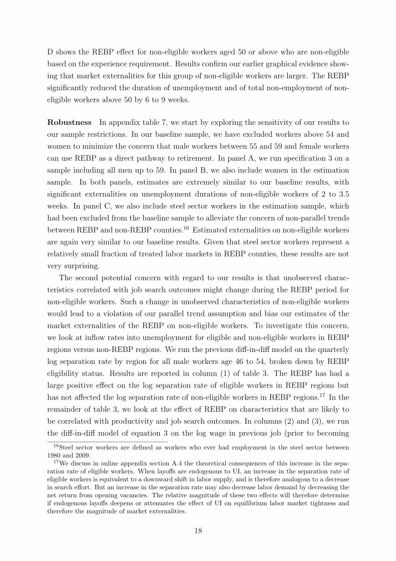
Robustness In appendix table 7, we start by exploring the sensitivity of our results to

our sample restrictions. In our baseline sample, we have excluded workers above 54 and

women to minimize the concern that male workers between 55 and 59 and female workers

can use REBP as a direct pathway to retirement. In panel A, we run specification 3 on a

sample including all men up to 59. In panel B, we also include women in the estimation

sample. In both panels, estimates are extremely similar to our baseline results, with

significant externalities on unemployment durations of non-eligible workers of 2 to 3.5

weeks. In panel C, we also include steel sector workers in the estimation sample, which

had been excluded from the baseline sample to alleviate the concern of non-parallel trends

between REBP and non-REBP counties.16 Estimated externalities on non-eligible workers

are again very similar to our baseline results. Given that steel sector workers represent a

relatively small fraction of treated labor markets in REBP counties, these results are not

very surprising.

The second potential concern with regard to our results is that unobserved charac-

teristics correlated with job search outcomes might change during the REBP period for

non-eligible workers. Such a change in unobserved characteristics of non-eligible workers

would lead to a violation of our parallel trend assumption and bias our estimates of the

market externalities of the REBP on non-eligible workers. To investigate this concern,

we look at inflow rates into unemployment for eligible and non-eligible workers in REBP

regions versus non-REBP regions. We run the previous diff-in-diff model on the quarterly

log separation rate by region for all male workers age 46 to 54, broken down by REBP

eligibility status. Results are reported in column (1) of table 3. The REBP has had a

large positive effect on the log separation rate of eligible workers in REBP regions but

has not affected the log separation rate of non-eligible workers in REBP regions.17 In the

remainder of table 3, we look at the effect of REBP on characteristics that are likely to

be correlated with productivity and job search outcomes. In columns (2) and (3), we run

the diff-in-diff model of equation 3 on the log wage in previous job (prior to becoming

16Steel sector workers are defined as workers who ever had employment in the steel sector between1980 and 2009.

17We discuss in online appendix section A.4 the theoretical consequences of this increase in the sepa-ration rate of eligible workers. When layoffs are endogenous to UI, an increase in the separation rate ofeligible workers is equivalent to a downward shift in labor supply, and is therefore analogous to a decreasein search effort. But an increase in the separation rate may also decrease labor demand by decreasing thenet return from opening vacancies. The relative magnitude of these two effects will therefore determineif endogenous layoffs deepens or attenuates the effect of UI on equilibrium labor market tightness andtherefore the magnitude of market externalities.

18

unemployed), controlling for observable characteristics. We cannot detect any effect of

the REBP program on the distribution of residual wages in previous job of non-eligible

workers in REBP regions. For eligible workers, there is a small though not significant

positive effect, which suggests that eligible unemployed who took up REBP had slightly

better wages in their previous job. In column (4) and (5) we look at the logarithm of

tenure in the previous job (prior to becoming unemployed). Again, we find almost no

effect for non-eligible workers and a small positive effect for eligible workers. Overall,

these findings alleviate the concern of an important change in unobserved characteristics

of non-eligible workers in REBP regions at the time of the REBP program.

The third concern with our baseline estimates is the possible presence of differential

region-specific shocks at the time the REBP program was in place. This concern is

valid given that REBP counties were not chosen at random but because of the relative

importance of their steel sector. Yet note that the fraction of steel sector employees never

exceeds 15% of the labor force in these counties, and we restrict our baseline sample to

individuals who never were employed in the steel sector. Also, because REBP counties

were experiencing a restructuring of the steel sector, we should expect the region-specific

shock to be negative during the REBP period for REBP counties, which would lead to

higher unemployment durations for non-eligible workers. In this sense, region-specific

shocks are likely, if anything, to bias downward the magnitude of our estimates of the

search externalities for non-eligible workers.

To further investigate the robustness of our results to the presence of region-specific

shocks, we use men below age 40 in REBP counties as a control, instead of workers from

non-REBP counties. To do so, we run on a sample restricted to unemployed aged 30 to

39 and 50 to 54 in REBP counties a diff-in-diff specification equivalent to equation (3)

where we replace M by A = 1[Age > 50]. This specification enables us to control for

shocks to the labor markets of REBP counties contemporaneous to the REBP that affect

all job seekers in the same way. Results are reported in appendix table 8. Estimated

externalities on non-eligible unemployed aged 50 to 54 are virtually unaffected compared

to table 2 panel D. This suggests that our estimated externalities are not driven by labor

market shocks specific to REBP counties and contemporaneous to the REBP period.

Treatment intensity The magnitude of market externalities depends on treatment

intensity, i.e. the relative size of the treated group of eligible unemployed compared to the

non-treated group of non-eligible workers (appendix A.2). To investigate how estimated

externalities vary with treatment intensity, we look at different measures of treatment

intensity and interact these measures with the REBP effect on non-eligible workers. The

19

estimated specification is

Yit = α + β0 ·H ·M · Tt + (γH0 · 1[Treat=High] + γL0 · 1[Treat=Low]) · (1−H) ·M · Tt+η0 ·M +

∑νt + η1 ·H+ η2 ·M ·H+

∑ιt ·H+X ′itρ+ εit

(4)

where 1[Treat=High] and 1[Treat=Low] are indicators for a proxy of treatment intensity

being above or below some threshold.

We use two methods to characterize treatment intensity. In the first method, we start

by computing the average quarterly fraction of new hires coming from non-REBP counties

among all new hires of men aged 46 to 54 for each REBP county when the REBP was

not in place as shown in figure 2 panel B. Counties that, absent REBP, had on average a

high fraction of hires coming from non-REBP regions have labor markets that are more

integrated to non-REBP regions and the REBP effect on aggregate search effort within

these counties is likely to be smaller than in counties that hardly ever hire individuals from

non-REBP regions. We define high treatment intensity counties as counties where the

fraction of new hires coming from non-REBP counties is lower than 5% which corresponds

to the median value across REBP counties. Table 4 panel A displays the results and shows

that the effect of REBP on non-eligible unemployed was significantly stronger in counties

with a low level of integration to non-REBP counties. REBP induced a reduction in non-

employment duration of non-eligible workers of only .7 weeks in low treatment counties

but of 4.2 weeks in high treatment counties. When zooming on non-eligible workers aged

50 and above, this pattern is even more striking, with a reduction in the average duration

of unemployment of 4 weeks for low treatment counties and of more than 10 weeks for

high treatment counties.

We confirm the robustness of these results using a second measure of treatment inten-

sity. We compute the average yearly fraction of eligible workers among the 50+ for each

region×industry×education cell during REBP years and define by high treatment inten-

sity a cell where the fraction of eligible 50+ unemployed was more than 90% (the median

value across all region×industry×education cells).18 Results are displayed in table 4 panel

B and confirm the pattern found using our first measure of treatment intensity. In low

treatment-intensity cells, the estimated externalities of REBP on non-eligible workers are

approximately two times smaller than in high treatment-intensity cells, and this pattern

is valid for all non-eligible workers, as well as for non-eligible workers above 50.

Landais, Michaillat and Saez [2010] show that in the presence of “job rationing”,

externalities should be larger when initial labor market tightness is low as job rationing

will be more intense, exacerbating the rat race effect. In appendix table 9 we therefore

also explore heterogeneity in estimated externalities with respect to the initial level of

18A region is defined as the first two digits of the municipality identifiers.

20

labor market tightness. Unfortunately, the first year for which we have some vacancy

information by county is 1990 and we cannot compute labor market tightness prior to

REBP. We compute initial labor market tightness as of 1990 by dividing the average

monthly number of vacancies posted in 1990 in each county×industry×education cell,

by the average monthly number of unemployed in the same county×industry×education

cell. And we define low tightness cells as county×industry×education cells where initial

tightness is below the median of initial tightness across all cells. Results, displayed in table

9, suggest that non-eligible workers in low tightness cells experienced significantly shorter

unemployment spells due to REBP than non-eligible workers in high initial tightness cells.

When focusing on non-eligible workers above 50, we also find strong suggestive evidence

that REBP externalities were significantly stronger in labor markets with low tightness

at the start of REBP.

Geographical spillovers So far, we have excluded from our sample unemployed resid-

ing in non-REBP counties that had labor markets highly integrated to REBP counties

before the REBP. These counties are likely to experience spillover effects from REBP

counties and cannot serve as a proper control in our diff-in-diff strategy. We now inves-

tigate directly whether we can detect the presence of REBP externalities on unemployed

workers residing in these counties. We begin by running a simple diff-in-diff specification

comparing unemployed workers residing in non-REBP counties with high integration to

REBP counties to unemployed workers residing in non-REBP counties with low level of

integration.19 We restrict our sample to male unemployed workers aged 50 to 54 with

more than 15 years of experience, who would be eligible to the REBP if residing in REBP

counties. Results are reported in panel A of table 5 and suggest that the REBP reduced

the duration of unemployment spells by 4 weeks for unemployed workers in non-REBP

counties with high labor market integration to REBP counties relative to similar workers

in non-REBP counties with little labor market integration to REBP counties.

In panel B of table 5, we use a finer measure of labor market integration by looking

at county×industry×education cells, and we compare unemployed workers in cells where

the average fraction of hires from REBP counties in total yearly hires was larger than

20% before the REBP to unemployed in cells where it was lower than 20%. Our estimates

show that the REBP significantly improved job search outcomes for unemployed workers

in cells where competition with REBP workers was the strongest: unemployed in these

cells experienced a decline in unemployment duration of 2.5 to 5 weeks relative to similar

workers residing in cells with low competition from REBP workers.

19High integration to REBP counties is defined as having an average quarterly fraction of new hirescoming from REBP regions in the total number of new hires above 15% for all non-REBP periods.

21

Wages The sign and magnitude of our estimated REBP market externalities suggest

that wages did not react much to outside options of eligible workers. Higher wages would

have triggered a decrease in the number of job vacancies opened by firms and would have

muted or even reversed the externalities on non-eligible workers. Here, we investigate

explicitly this question by looking at the REBP effect on reemployment wages of eligible

workers.

Analyzing the REBP effect on wages is very different from our previous market ex-

ternality analysis, as we now wish to compare eligible workers to non-eligible workers.

Identification of the effect on wages is difficult for at least three reasons. First, the REBP

increases unemployment duration for eligible workers, which may directly affect wages

through duration dependence effects. Second, REBP treatment affects the probability of

entering into unemployment and REBP recipients may therefore be selected along unob-

served characteristics that are correlated with wages. Treatment is also correlated with

the probability of ever reentering the labor force, which creates additional selection issues.

Finally, the REBP affects labor market tightness, which will in turn affect the bargaining

power of workers.

Given these difficulties, our analysis remains tentative and most of the details and

caveats are discussed more extensively in appendix section D. We start by comparing

eligible workers in REBP counties and non-REBP counties. Because eligible workers

in REBP counties experienced longer unemployment durations during the REBP than

eligible workers in non-REBP counties, reemployment wages of eligible workers in REBP

and non-REBP counties may simply differ because of variations in the distribution of wage

offers over the duration of a spell. To control for this issue, we follow the methodology

of Schmieder, von Wachter and Bender [2012a] and estimate the effect of variations in

benefits on reemployment wages holding unemployment duration constant. Identification

is based on the assumption that there is no correlation between unobserved heterogeneity

and unemployment benefits conditional on unemployment duration.

We plot in appendix figure 6 post-unemployment wages conditional on the duration of

the unemployment spell in REBP and non-REBP counties for eligible workers (aged 50 to

54 with more than 15 years of experience). The difference between REBP and non-REBP

counties at each duration point in panel B (when REBP was in place) compared to the

same difference in panel A (when REBP was not in place) gives us a diff-in-diff estimate

of the REBP effect on reemployment wages conditional on spell duration. This evidence

suggests that there was no significant REBP effect on reemployment wages.

We formally assess this result in appendix table 10 by running a simple diff-in-diff

model where we compare workers eligible to the REBP (treatment) to non-eligible workers

(control). Each panel uses a different control group. In panel A, we use workers aged 50

to 54 with more than 15 years of experience but residing in non-REBP regions. In panel

B we use workers aged 50 to 54 residing in REBP regions but with less than 15 years

22

of experience. In panel C we use workers aged 46 to 49 with 15 years of experience and

residing in REBP regions. In our preferred specification of column (4), we condition on the

duration of unemployment using a rich set of dummies for the duration of unemployment

prior to finding a new job. Irrespective of the control group we are using, we always find

no significant REBP effect on reemployment wages.20

Overall, this evidence, although tentative, suggests that wages of eligible workers did

not strongly respond to the REBP, which is in line with the market externalities that we

find. Yet, we cannot exclude that these results are confounded by selection, nor can we

exclude that wages would have adjusted in the very long run.

V Discussion and policy implications

Micro versus macro effects of UI extensions Our empirical findings have important

policy implications. The overall effect of a change in UI on the job finding rate (the

macro effect of UI), is the sum of the micro effect and of market externalities. The

presence of significant market externalities implies that the micro and the macro effect of

UI extensions are not the same. Estimates of the effects of UI benefits on search effort

using variation in UI across individuals within a labor market capture micro effects of UI

and do not provide enough information to assess the full welfare implications of variations

in UI benefits.

Importantly, our analysis also offers direct insights on the relative magnitude of micro

and macro effects of variations in benefits in a labor market. We are interested in recov-

ering the wedge between micro and macro effects when changing UI for the whole labor

market. This wedge is W = 1 − eM/em where eM is the total effect on job finding rate

of treating the whole market by an increase dB in UI benefits (“macro effect”) and em is

the “micro effect”. This wedge can be recovered from our two groups quasi-experimental

setting (appendix A.2):

W =

1pdDbdBa

dDadBa− dDb

dBa

(5)

The numerator dDbdBa

is the effect of the REBP increase in UI, dBa, for eligible workers on

the duration of unemployment of non-eligible workers, Db, and captures REBP market

externalities. Intuitively, because the effect of REBP on non-treated workers will create

externalities that are smaller than if the whole market was treated, one needs to rescale

20To complement our diff-in-diff approach, in appendix D we also exploit the age eligibility discontinuityat 50 and the experience eligibility discontinuity in REBP counties to estimate RD effects of the REBPextensions controlling for the effect of duration on reemployment wages by adding a rich set of dummiesfor the duration of the spell prior to finding the job. Results suggest the presence of no wage effectusing the experience discontinuity, and a small significant elasticity of wages with respect to UI benefitswhen using the age discontinuity. Note however that the McCrary test strongly rejects continuity in theprobability density function of age) at the cutoff (50 years) during the REBP period, which suggests thatthe estimated wage effects could partly be driven by selection (sorting) at the 50 years age cut-off.

23

estimated externalities in our experiment by 1/p where p is the fraction of eligible workers

in the market. The denominator is the micro effect of REBP. It is equal to the total effect

of REBP on the spell duration of eligible workers dDadBa

minus REBP externalities identified

by dDbdBa

.

We can now calibrate the wedge W of equation (5) for the labor market of eligible 50

to 54 in REBP regions. To calibrate the numerator dDbdBa

, we use the externalities estimate

γ0 of table 2 column (4) for non-eligible workers aged 50 to 54: γ0 = −6.91. These non-

eligible workers are the most likely to be competing in the same labor market as eligible

workers and of capturing the full extent of externalities in this labor market. For dDadBa

, we

use the estimate of the full effect of REBP on eligible workers β0 from table 2 column (4):

β0 = −29.17. For p, we use the average fraction of eligible workers among 50-54 workers

in REBP regions prior to REBP ≈ .9. This gives us a wedge of W ≈ .21.

To what extent is this wedge informative about the micro and macro effects of treat-

ing all labor markets by having a country-wide or region-wide unemployment insurance

extension? To answer this question, it is important to realize that, compared to a setting

where all labor markets would be treated, in the REBP setting, some untreated labor

markets (for workers aged below 50 for instance) are offering substitution opportunities

to treated workers. We explain in appendix section A.3 the consequences of the existence

of substitution possibilities across markets on the magnitude of market externalities of

UI. The intuition is that when the treated labor market is small, and the elasticity of

substitution with workers from other markets is large, then the treated market is like a

small open economy: its labor market tightness is close to infinitely elastic and set by the

labor market tightness of substitution markets. Labor market tightness in the treated

market will therefore not react strongly to variations in UI for workers in that market and

market externalities of UI will be small. In other words, the more substitutes are available

for firms, the smaller the market externalities of UI in the treated market. This suggests

that the wedge between the micro and macro effects of country-wide or region-wide UI

extensions could be greater than the wedge we found in the REBP context for the treated

market of male workers aged 50 to 54.

Implications for welfare effects of UI extensions Our results bear important im-

plications for optimal UI policies. As explained in Landais, Michaillat and Saez [2010], in

equilibrium search and matching models, the traditional partial equilibrium Baily-Chetty

formula for the optimal level of benefits (Chetty [2006]) needs to be extended to take

into account the difference between partial equilibrium (micro) and macro effects of UI

benefits which captures equilibrium adjustments in labor market tightness. The reason is

that, when the Hosios condition does not hold and the economy is inefficient, UI-induced

variations in labor market tightness will have first-order welfare effects by affecting work-

ers’ job-finding probability per unit of effort. When the economy is slack, more UI is

24

desirable if UI increases tightness and less UI is desirable if UI decreases tightness.

Given that we find a positive wedge between the micro and the macro effects, this

implies that more generous UI increases labor market tightness. As a consequence, the

optimal level of UI will be larger than suggested by the partial equilibrium Baily-Chetty

formula. UI extensions are less distortionary than based on estimation of micro estimates

of the effects of UI.

Our results in appendix table 9 further suggest that market externalities are larger

when initial labor market tightness is low. This would imply that the wedge between micro

and macro effects is likely to be larger during recessions (low tightness) than during booms

(high tightness). This would therefore offer a natural justification for countercyclical

extensions of UI on efficiency grounds, as hypothesized in Landais, Michaillat and Saez

[2010].

Market externalities are likely to be larger in the short run. There are two potential

reasons for this. First, in the short run, returns to labor are more likely to be decreasing

(capital not being able to adjust as quickly as labor fluctuations). Second, because of

various frictions in the wage-setting process, it might take time for wages to adjust to a

change in UI benefits. Our empirical evidence nevertheless suggests that even after three

to four years, positive REBP externalities are still detectable on non-eligible workers. Be-

cause the REBP program was only temporary, we cannot properly estimate the speed at

which externalities may decrease over time. In the long run, however, it is possible that

these externalities would have decreased. First, because, as suggested by appendix figure

7, it seems that wages started to react more to REBP extensions over time. Second, in

the long run, labor demand is likely to become more elastic to labor market tightness

as returns to labor are more likely to become constant. Eventually, it is even possible

that externalities change sign in the long run, so that the macro effect of UI variations

becomes larger than the micro effect.21 In terms of policy implications, this means that

temporary extensions enacted in reaction to business cycles downturns are less socially

costly than previously thought. And when determining the optimal time span of tempo-

rary extensions, governments should pay attention to the evolution of market externalities

over time.

21This may explain why cross-sectional estimates comparing countries or US states tend to find muchlarger elasticities than reform-based (short term) estimates. This may also explain why, European coun-tries with generous UI coverage experience high level of structural long term unemployment despite thefact that most reform-based estimates in Europe find relatively modest elasticities in the short run.

25

References

Blundell, Richard, Monica Costa Dias, Costas Meghir, and John Van Reenen.

2004. “Evaluating the Employment Impact of a Mandatory Job Search Program.” Jour-

nal of the European Economic Association, 2(4): 569–606.

Chetty, Raj. 2006. “A General Formula for the Optimal Level of Social Insurance.”

Journal of Public Economics, 90(10-11): 1879–1901.

Chetty, Raj, John N. Friedman, Soren Leth-Petersen, Torben Nielsen, and

Tore Olsen. 2014. “Active vs. Passive Decisions and Crowdout in Retirement Savings

Accounts: Evidence from Denmark.” The Quarterly Journal of Economics, forthcom-

ing.

Conley, T.G. 1999. “GMM estimation with cross sectional dependence.” Journal of

Econometrics, 92(1): 1 – 45.

Crepon, Bruno, Esther Duflo, Marc Gurgand, Roland Rathelot, and Philippe

Zamora. 2013. “Do Labor Market Policies have Displacement Effects? Evidence from a

Clustered Randomized Experiment.” The Quarterly Journal of Economics, 128(2): 531–

580.

Ferracci, Marc, Gregory Jolivet, and Gerard J. van den Berg. 2010. “Treatment

Evaluation in the Case of Interactions within Markets.” Institute for the Study of Labor

(IZA) IZA Discussion Paper 4700.

Gautier, Pieter, Paul Muller, Bas van der Klaauw, Michael Rosholm, and

Michael Svarer. 2012. “Estimating Equilibrium Effects of Job Search Assistance.”

Tinbergen Institute Tinbergen Institute Discussion Papers 12-071/3.

Hagedorn, Marcus, and Iourii Manovskii. 2008. “The Cyclical Behavior of

Equilibrium Unemployment and Vacancies Revisited.” American Economic Review,

98(4): 1692–1706.

Hagedorn, Marcus, Fatih Karahan, Iourii Manovskii, and Kurt Mitman. 2013.

“Unemployment Benefits and Unemployment in the Great Recession: The Role of

Macro Effects.” National Bureau of Economic Research, Inc NBER Working Papers

19499.

Inderbitzin, Lukas, Stefan Staubli, and Josef Zweimuller. 2013. “Extended Un-

employment Benefits and Early Retirement: Program Complementarity and Program

Substitution.” Institute for the Study of Labor (IZA) IZA Discussion Paper 7330.

Kline, Patrick, and Enrico Moretti. 2014. “Local Economic Development, Agglom-

eration Economies, and the Big Push: 100 Years of Evidence from the Tennessee Valley

Authority.” Quarterly Journal of Economics, forthcoming.

Krueger, Alan B., and Bruce D. Meyer. 2002. “Labor supply effects of social insur-

26

ance.” Elsevier Handbook of Public Economics.

Lalive, Rafael. 2007. “Unemployment Benefits, Unemployment Duration, and Post-

Unemployment Jobs: A Regression Discontinuity Approach.” American Economic Re-

view, 97(2): 108–112.

Lalive, Rafael. 2008. “How do extended benefits affect unemployment duration A re-

gression discontinuity approach.” Journal of Econometrics, 142(2): 785–806.

Lalive, Rafael, and Josef Zweimuller. 2004a. “Benefit Entitlement and the Labor

Market: Evidence from a Large-Scale Policy Change.” In Labor Market Institutions

and Public Policy. , ed. Jonas Agell, Michael Keen and Alfons Weichenrieder, 63–100.

Cambridge, Massachusetts: MIT Press.

Lalive, Rafael, and Josef Zweimuller. 2004b. “Benefit Entitlement and Unem-

ployment Duration: The Role of Policy Endogeneity.” Journal of Public Economics,

88(12): 2587–2616.

Lalive, Rafael, Jean-Philippe Wuellrich, and Josef Zweimueller. 2013. “Do Finan-

cial Incentives Affect Firms Demand For Disabled Workers?” Journal of the European

Economic Association, 11(1): 25–58.

Landais, Camille. 2013. “Assessing theWelfare Effects of Unemployment Benefits Using

the Regression Kink Design.” London School of Economics, PEP working paper.

Landais, Camille, Pascal Michaillat, and Emmanuel Saez. 2010. “Optimal Unem-

ployment Insurance over the Business Cycle.” National Bureau of Economic Research

Working Paper 16526.

Leoni, Thomas, and Wolfgang Pollan. 2011. “Lohnentwicklung und Lohnunter-

schiede in der Industrie seit 2000.” WIFO WIFO Monatsberichte.

Levine, Phillip B. 1993. “Spillover Effects between the Insured and Uninsured Unem-

ployed.” Industrial and Labor Relations Review, 47(1): pp. 73–86.

Marinescu, Ioana. 2014. “The General Equilibrium Impacts of Unemployment Insur-

ance: Evidence from a Large Online Job Board.” University of Chicago mimeo.

Michaillat, Pascal. 2012. “Do Matching Frictions Explain Unemployment? Not in Bad

Times.” American Economic Review, 102(4): 1721–50.

Schmieder, Johannes F., Till von Wachter, and Stefan Bender. 2012a. “The

Effect of Unemployment Insurance Extensions on Reemployment Wages.” Mimeo.

Schmieder, Johannes F., Till von Wachter, and Stefan Bender. 2012b. “The Ef-

fects of Extended Unemployment Insurance Over the Business Cycle: Evidence from

Regression Discontinuity Estimates Over 20 Years.” The Quarterly Journal of Eco-

nomics, 127(2): 701–752.

Shimer, Robert. 2004. “Search Intensity.” https://sites.google.com/site/

robertshimer/intensity.pdf.

27

Shimer, Robert. 2005. “The Cyclical Behavior of Equilibrium Unemployment and Va-

cancies.” American Economic Review, 95(1): 25–49.

Winter-Ebmer, Rudolf. 1996. “Benefit Duration and Unemployment Entry: Quasi-

experimental Evidence for Austria.” C.E.P.R. Discussion Papers CEPR Discussion Pa-

pers 1521.

Zweimuller, Josef, Rudolf Winter-Ebmer, Rafael Lalive, Andreas Kuhn, Jean-

Philippe Wuellrich, Oliver Ruf, and Simon Buchi. 2009. “Austrian Social Se-

curity Database.” The Austrian Center for Labor Economics and the Analysis of the

Welfare State, Johannes Kepler University Linz, Austria NRN working paper 2009-03.

28

Figure 1: Evaluating the degree of competition for identical vacancies be-tween REBP eligible workers and different groups of non-eligible work-ers:

A. Goodness-of-fit tests0

.2.4

.6.8

1P-

valu

e of

Chi

-2 te

st

35-40 vs 50-54years old

40-45 vs 50-54years old

45-50 vs 50-54years old

Non-eligible 50+vs 50-54years old

P-value of Pearson's Chi-2 testP-value of Hosmer-Lemeshow Chi-2 test

B. Fraction of misclassified observations & fraction of type I errors

0.1

.2.3

Frac

tion

of ty

pe I

erro

r

0.1

.2.3

Frac

tion

of o

bser

vatio

ns in

corre

ctly

spe

cifie

d

35-40 vs 50-54years old

40-45 vs 50-54years old

45-50 vs 50-54years old

Non-eligible 50+vs 50-54years old

Fraction of observations incorrectly specifiedFraction of type I errors

Notes:This figure reports various goodness-of-fit measures of a logit model where the REBP-eligibility status of the worker filling a vacancyis explained by all the characteristics of the vacancy. We estimate this model separately for different groups of non-eligible workers againsteligible workers. A good fit of the model indicates that non-eligible workers fill vacancies that are very different from the vacancies filled byeligible workers. A poor goodness-of-fit indicates that eligible and non-eligible workers fill vacancies that have very similar characteristics. Inpanel A, we plot the p-value of two standard goodness-of-fit tests for the logit model, the Pearson’s χ2 goodness of fit test and the Hosmer-Lemeshow χ2 goodness of fit test. A low p-value indicates poor fit and low predictive value of the model. In panel B, we plot the fractionof observations that are misclassified by our model (the predicted status is different from the true status of the worker filling the vacancy).We also plot the fraction of type I errors of the model. The classification error measures of panel B should be interpreted with caution asclassification is sensitive to the relative sizes of each group of workers. We therefore tend to prefer goodness-of-fit measures presented in panelA. All the details are given in the online appendix section B.

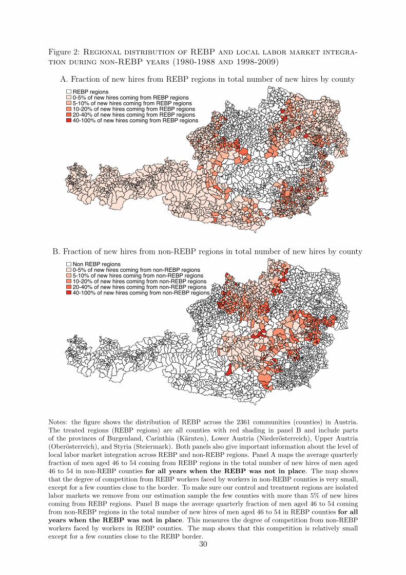
Figure 2: Regional distribution of REBP and local labor market integra-tion during non-REBP years (1980-1988 and 1998-2009)

A. Fraction of new hires from REBP regions in total number of new hires by county

REBP regions0-5% of new hires coming from REBP regions5-10% of new hires coming from REBP regions10-20% of new hires coming from REBP regions20-40% of new hires coming from REBP regions40-100% of new hires coming from REBP regions

B. Fraction of new hires from non-REBP regions in total number of new hires by county

Non REBP regions0-5% of new hires coming from non-REBP regions5-10% of new hires coming from non-REBP regions10-20% of new hires coming from non-REBP regions20-40% of new hires coming from non-REBP regions40-100% of new hires coming from non-REBP regions

Notes: the figure shows the distribution of REBP across the 2361 communities (counties) in Austria.The treated regions (REBP regions) are all counties with red shading in panel B and include partsof the provinces of Burgenland, Carinthia (Karnten), Lower Austria (Niederosterreich), Upper Austria(Oberosterreich), and Styria (Steiermark). Both panels also give important information about the level oflocal labor market integration across REBP and non-REBP regions. Panel A maps the average quarterlyfraction of men aged 46 to 54 coming from REBP regions in the total number of new hires of men aged46 to 54 in non-REBP counties for all years when the REBP was not in place. The map showsthat the degree of competition from REBP workers faced by workers in non-REBP counties is very small,except for a few counties close to the border. To make sure our control and treatment regions are isolatedlabor markets we remove from our estimation sample the few counties with more than 5% of new hirescoming from REBP regions. Panel B maps the average quarterly fraction of men aged 46 to 54 comingfrom non-REBP regions in the total number of new hires of men aged 46 to 54 in REBP counties for allyears when the REBP was not in place. This measures the degree of competition from non-REBPworkers faced by workers in REBP counties. The map shows that this competition is relatively smallexcept for a few counties close to the REBP border.

30

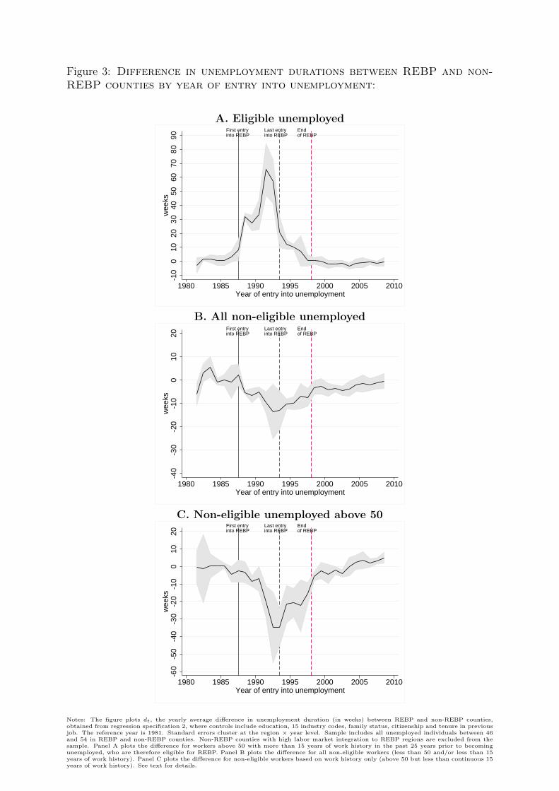
Figure 3: Difference in unemployment durations between REBP and non-REBP counties by year of entry into unemployment:

A. Eligible unemployedFirst entryinto REBP

Last entryinto REBP

Endof REBP

-10

010

2030

4050

6070

8090

wee

ks

1980 1985 1990 1995 2000 2005 2010Year of entry into unemployment

B. All non-eligible unemployedFirst entryinto REBP

Last entryinto REBP

Endof REBP

-40

-30

-20

-10

010

20w

eeks

1980 1985 1990 1995 2000 2005 2010Year of entry into unemployment

C. Non-eligible unemployed above 50First entryinto REBP

Last entryinto REBP

Endof REBP

-60

-50

-40

-30

-20

-10

010

20w

eeks

1980 1985 1990 1995 2000 2005 2010Year of entry into unemployment

Notes: The figure plots dt, the yearly average difference in unemployment duration (in weeks) between REBP and non-REBP counties,obtained from regression specification 2, where controls include education, 15 industry codes, family status, citizenship and tenure in previousjob. The reference year is 1981. Standard errors cluster at the region × year level. Sample includes all unemployed individuals between 46and 54 in REBP and non-REBP counties. Non-REBP counties with high labor market integration to REBP regions are excluded from thesample. Panel A plots the difference for workers above 50 with more than 15 years of work history in the past 25 years prior to becomingunemployed, who are therefore eligible for REBP. Panel B plots the difference for all non-eligible workers (less than 50 and/or less than 15years of work history). Panel C plots the difference for non-eligible workers based on work history only (above 50 but less than continuous 15years of work history). See text for details.

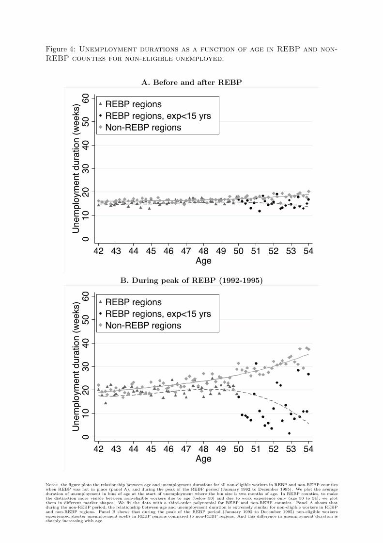
Figure 4: Unemployment durations as a function of age in REBP and non-REBP counties for non-eligible unemployed:

A. Before and after REBP0

1020

3040

5060

Une

mpl

oym

ent d

urat

ion

(wee

ks)

42 43 44 45 46 47 48 49 50 51 52 53 54Age

REBP regionsREBP regions, exp<15 yrsNon-REBP regions

B. During peak of REBP (1992-1995)

010

2030

4050

60U

nem

ploy

men

t dur

atio

n (w

eeks

)

42 43 44 45 46 47 48 49 50 51 52 53 54Age

REBP regionsREBP regions, exp<15 yrsNon-REBP regions

Notes: the figure plots the relationship between age and unemployment durations for all non-eligible workers in REBP and non-REBP countieswhen REBP was not in place (panel A), and during the peak of the REBP period (January 1992 to December 1995). We plot the averageduration of unemployment in bins of age at the start of unemployment where the bin size is two months of age. In REBP counties, to makethe distinction more visible between non-eligible workers due to age (below 50) and due to work experience only (age 50 to 54), we plotthem in different marker shapes. We fit the data with a third-order polynomial for REBP and non-REBP counties. Panel A shows thatduring the non-REBP period, the relationship between age and unemployment duration is extremely similar for non-eligible workers in REBPand non-REBP regions. Panel B shows that during the peak of the REBP period (January 1992 to December 1995) non-eligible workersexperienced shorter unemployment spells in REBP regions compared to non-REBP regions. And this difference in unemployment duration issharply increasing with age.

Table 1: Summary statistics

(1) (2) (3) (4) (5) (6) (7) (8)

A. REBP vs non-REBP countiesNon-REBP period REBP period

Non-REBP REBP Non-REBP REBPcounties counties Difference p-value counties counties Difference p-value

Fraction employed in the steel sector .055 .152 -.097 0 .057 .156 -.099 0Monthly 46-54 unemployment rate .055 .054 .001 .864 .073 .113 -.04 0Fraction eligible to REBP .382 .396 -.014 0 .449 .533 -.084 0Age 49.7 49.7 0 .343 49.8 50.1 -.3 0Unemployment duration 13.6 14.3 -.7 0 15.9 29 -13.1 0Non employment duration 22.7 21.2 1.4 0 32.9 45.4 -12.4 0Wage before U spell (e2000) 13448 14306 -857 0 13122 14498 -1375 0

B. Eligible vs non-eligible unemployed in REBP countiesNon-REBP period REBP period

Non-eligible Eligible Non-eligible Eligibleunemployed unemployed Difference p-value unemployed unemployed Difference p-value

Age 48.2 51.9 -3.7 0 48 52 -4 0Unemployment duration 17.5 20.8 -3.2 0 23.2 88.8 -65.6 0Non employment duration 21.6 24.7 -3.1 0 31.4 99.6 -68.2 0Wage before U spell (e2000) 14096 14623 -527 0 13316 15549 -2232 0Fraction with compulsory education .529 .501 .028 0 .511 .506 .005 .44Fraction married .744 .751 -.007 .076 .748 .803 -.055 0

Notes: The table displays summary statistics from the Austrian social security and unemployment insurance files. Panel A compares REBP and non-REBP counties in the non-REBP period (1980 to May 1988 andAugust 1997 to 2009) and during the REBP period (June 1988 to July 1997). P-value is for a test of equality of means for REBP and non-REBP counties. The fraction of employment in the steel sector is defined as theaverage quarterly fraction of individuals aged 46 to 54 employed in the steel industry. The unemployment rate is the average monthly number of unemployed men aged 46 to 54 recorded in the unemployment insurancefiles as a fraction of the sum of unemployed and employed male workers aged 46 to 54. All remaining rows in this table are computed for our estimation sample of unemployed workers which is restricted to men, aged46 to 54, who never work in the steel sector. Panel B compares, in REBP counties, in the non-REBP period (1980 to May 1988 and August 1997 to 2009) and during the REBP period (June 1988 to July 1997), eligibleunemployed workers (above 50 and with more than 15 years of continuous work history in the past 25 years) to non-eligible unemployed workers (with less than 15 years of continuous work history in the past 25 yearsor below 50). P-value is for a test of equality of means for these two groups. All duration outcomes are expressed in weeks. Wages are annually adjusted and expressed in constant e2000. Non-employment is defined asthe number of weeks between two employment spells. Unemployment duration is the duration of paid unemployment recorded in the UI administrative data.

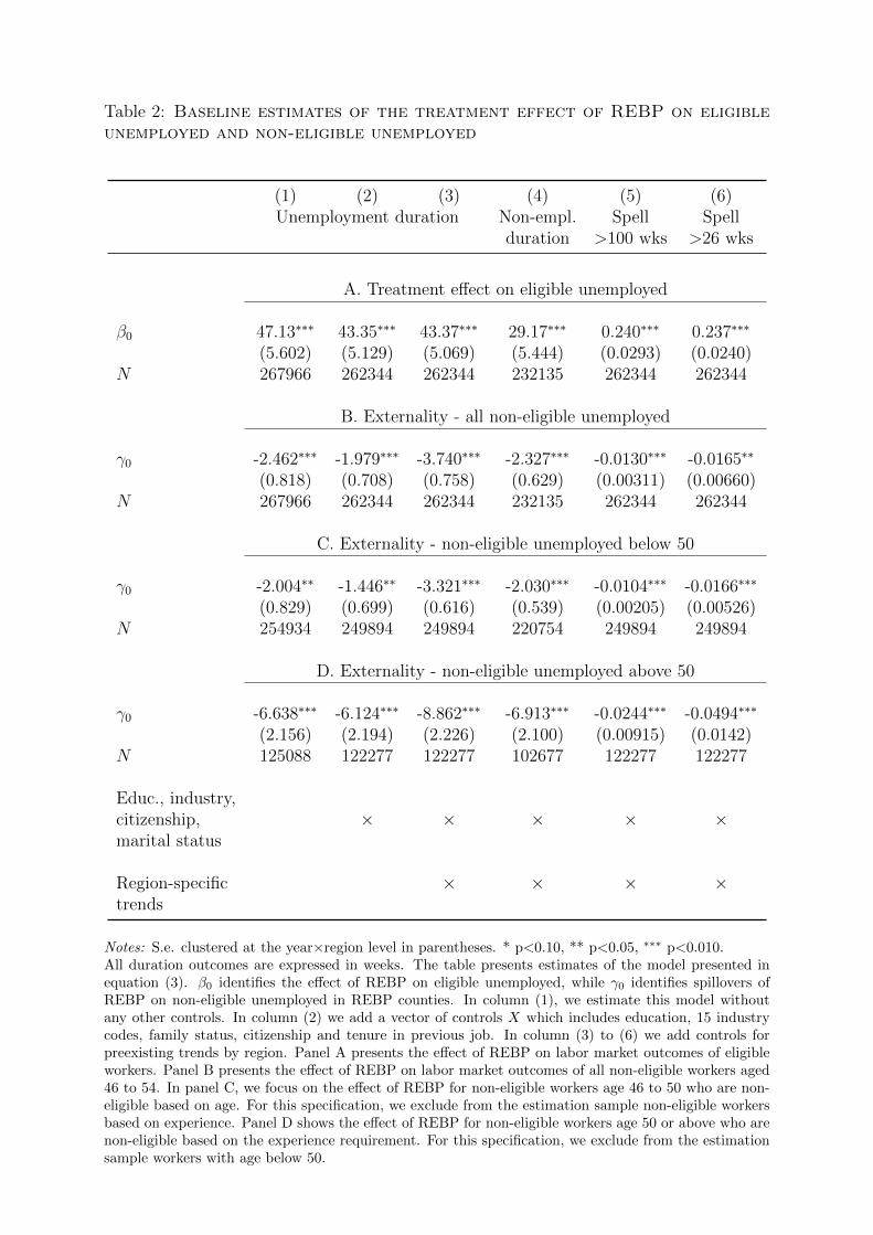
Table 2: Baseline estimates of the treatment effect of REBP on eligibleunemployed and non-eligible unemployed

(1) (2) (3) (4) (5) (6)Unemployment duration Non-empl. Spell Spell

duration >100 wks >26 wks

A. Treatment effect on eligible unemployed

β0 47.13∗∗∗ 43.35∗∗∗ 43.37∗∗∗ 29.17∗∗∗ 0.240∗∗∗ 0.237∗∗∗

(5.602) (5.129) (5.069) (5.444) (0.0293) (0.0240)N 267966 262344 262344 232135 262344 262344

B. Externality - all non-eligible unemployed

γ0 -2.462∗∗∗ -1.979∗∗∗ -3.740∗∗∗ -2.327∗∗∗ -0.0130∗∗∗ -0.0165∗∗

(0.818) (0.708) (0.758) (0.629) (0.00311) (0.00660)N 267966 262344 262344 232135 262344 262344

C. Externality - non-eligible unemployed below 50

γ0 -2.004∗∗ -1.446∗∗ -3.321∗∗∗ -2.030∗∗∗ -0.0104∗∗∗ -0.0166∗∗∗

(0.829) (0.699) (0.616) (0.539) (0.00205) (0.00526)N 254934 249894 249894 220754 249894 249894

D. Externality - non-eligible unemployed above 50

γ0 -6.638∗∗∗ -6.124∗∗∗ -8.862∗∗∗ -6.913∗∗∗ -0.0244∗∗∗ -0.0494∗∗∗

(2.156) (2.194) (2.226) (2.100) (0.00915) (0.0142)N 125088 122277 122277 102677 122277 122277

Educ., industry,citizenship, × × × × ×marital status

Region-specific × × × ×trends

Notes: S.e. clustered at the year×region level in parentheses. * p<0.10, ** p<0.05, ∗∗∗ p<0.010.All duration outcomes are expressed in weeks. The table presents estimates of the model presented inequation (3). β0 identifies the effect of REBP on eligible unemployed, while γ0 identifies spillovers ofREBP on non-eligible unemployed in REBP counties. In column (1), we estimate this model withoutany other controls. In column (2) we add a vector of controls X which includes education, 15 industrycodes, family status, citizenship and tenure in previous job. In column (3) to (6) we add controls forpreexisting trends by region. Panel A presents the effect of REBP on labor market outcomes of eligibleworkers. Panel B presents the effect of REBP on labor market outcomes of all non-eligible workers aged46 to 54. In panel C, we focus on the effect of REBP for non-eligible workers age 46 to 50 who are non-eligible based on age. For this specification, we exclude from the estimation sample non-eligible workersbased on experience. Panel D shows the effect of REBP for non-eligible workers age 50 or above who arenon-eligible based on the experience requirement. For this specification, we exclude from the estimationsample workers with age below 50.

Table 3: Testing for selection: impact of REBP on inflow rate into unem-ployment, log real wage in previous job and log tenure in previous jobof eligible and non-eligible unemployed

(1) (2) (3) (4) (5)log separation log real wage log tenure

rate in previous job in previous job

Eligible workers 0.286***(0.0356)

Non-eligible workers 0.0162(0.0218)

β0 (REBP effect on eligible) 0.109 0.128* 0.646*** 0.487***(0.0688) (0.0686) (0.0767) (0.0563)

γ0 (REBP effect on non-eligible) 0.0110 -0.00873 -0.0450 -0.0581*(0.0112) (0.0108) (0.0355) (0.0305)

Educ., marital status,industry, citizenship × ×

N 3390 240947 240923 267929 267901

Notes: For columns (2) to (5), standard errors are clustered at the year×region level. * p<0.10, **p<0.05, *** p<0.010. The table investigates the presence of selection effects of the REBP programaffecting the distribution of unobserved characteristics of non-eligible workers in REBP regions. Column(1) presents the diff-in-diff effect of the REBP program on the quarterly log separation rate of eligibleand non-eligible workers in REBP regions compared to non-REBP regions. In this column, observationsare at the eligibility group×region×quarter level. In columns (2) to (5), sample include all unemployedage 46 to 54. Columns (2) and (3) present specifications similar to that of table 2 but where the outcomevariable is the log wage in the previous job prior to becoming unemployed. Columns (4) and (5) repeatthe same regressions using the log tenure in previous job as an outcome.

35

Table 4: Externalities on non-eligible unemployed by REBP-treatment in-tensity

(1) (2) (3) (4)Unemployment Non-empl. Spell Spell

REBP effect on non-treated duration duration >100 wks >26 wks

A. Treatment intensity - Method 1:County share of hires from non-REBP counties

All non-eligibleγL0 (share of non-REBP hires > .05) -1.599** -0.676 -0.00275 -0.00289

(0.747) (0.693) (0.00224) (0.00661)γH0 (share of non-REBP hires ≤ .05) -2.866*** -4.170*** -0.00612* -0.0266***

(0.844) (0.917) (0.00324) (0.00733)F-Test γL0 = γH0 [0.0674] [0.0001] [0.138] [0.0002]

Non-eligible 50+γL0 (share of non-REBP hires > .05) -4.048** -4.191* -0.00300 -0.0119

(1.894) (2.309) (0.00788) (0.0136)γH0 (share of non-REBP hires ≤ .05) -15.24*** -10.66* -0.0519** -0.111***

(5.164) (5.831) (0.0230) (0.0372)F-Test γL0 = γH0 [0.0245] [0.310] [0.0354] [0.00566]

B. Treatment intensity - Method 2:Fraction treated in region×education×industry cell

All non-eligibleγL0 (fraction treated ≤ .9) -0.849 -1.022 0.00426 -0.00918

(0.933) (1.161) (0.00421) (0.00886)γH0 (fraction treated > .9 ) -2.238*** -1.908** -0.00560* -0.0102

(0.828) (0.802) (0.00307) (0.00725)F-Test γL0 = γH0 [0.252] [0.545] [0.104] [0.928]

Non-eligible 50+γL0 (fraction treated ≤ .9) -4.207 -3.661 -0.00126 -0.0351*

(2.807) (2.378) (0.0110) (0.0188)γH0 (fraction treated > .9) -8.831*** -8.022*** -0.0274*** -0.0235

(2.016) (2.426) (0.00952) (0.0215)F-Test γL0 = γH0 [0.0789] [0.0503] [0.0272] [0.668]

Educ., marital status,industry, citizenship × × × ×

Notes: S.e. clustered at the year×region level in parentheses. * p<0.10, ** p<0.05, *** p<0.010.Sample restricted to male workers working in non-steel related sectors. All duration outcomes are expressed in weeks. The tablepresents estimates of the effects of REBP on non-eligible workers broken down by REBP-treatment intensity. The estimatedspecification is that of equation (4). γH0 identifies spillovers of REBP on non-treated workers in high REBP-treatment intensityregions, γL0 identifies spillovers of REBP on non-treated workers in low REBP-treatment intensity regions. We use two methods tocharacterize treatment intensity. Method 1 computes the average quarterly fraction of new hires coming from non-REBP countiesfor each REBP county when the REBP was not in place and we define high treatment intensity counties as counties where thefraction of new hires coming from non-REBP counties is lower than 5%, which corresponds to the median value across REBPcounties. Method 2 computes the average yearly fraction of eligible workers among the 50+ for each region×industry×educationcell during REBP years and we define high treatment intensity as being in a cell where more than 90% of the 50+ unemployedwere eligible, which is the median value across all region×industry×education cells. A region is defined as the first two digits ofthe municipality identifiers.

Table 5: Geographical spillovers: Effect of REBP on unemployed work-ers in non-REBP counties with high labor market integration to REBPcounties

(1) (2) (3) (4) (5)Unemployment Non-empl. Spell Spell

duration duration >100 wks >26 wks

Labor market integration - Measure 1:Fraction of hires coming from REBP regions

in county cell

γ0 (geographical spillovers) -3.997*** -3.500** -1.043 -0.00658 -0.0239**(1.428) (1.440) (1.439) (0.00558) (0.0119)

Labor market integration - Measure 2:Fraction of hires coming from REBP regions

in county×industry×education cell

γ0 (geographical spillovers) -6.373*** -5.242*** -2.515*** -0.0141*** -0.0169***(1.213) (1.109) (0.659) (0.00368) (0.00603)

Educ., marital status,industry, citizenship × × × ×

N 104881 102840 88702 102840 102840

Notes: S.e. clustered at the year×region level in parentheses. * p<0.10, ** p<0.05, *** p<0.010.Sample restricted to male workers aged 50-54 working in non-steel related sectors with more than 15 yearsof experience in the past 25 years prior to becoming unemployed. All duration outcomes are expressed inweeks. The table presents estimates of a simple diff-in-diff specification comparing unemployed workersin non-REBP counties with high integration to REBP counties versus unemployed workers in non-REBPcounties with low level of integration as a control. In panel A, counties with high level of labor marketintegration are defined as counties with an average quarterly fraction of new hires coming from REBPregions in total number of new hires above 15% for all years when REBP was not in place. In panelB, we use a finer measure of labor market integration by looking at county×industry×education cells,and we compare unemployed workers in cells where the average fraction of hires from REBP counties intotal yearly hires was larger than 20% (for all years when REBP was not in place) to unemployed in cellswhere it was lower than 20%.

37

Online appendix

“Market Externalities of Large Unemployment Insur-

ance Extension Programs” by Lalive, Landais & Zweimuller

Not for publication

38

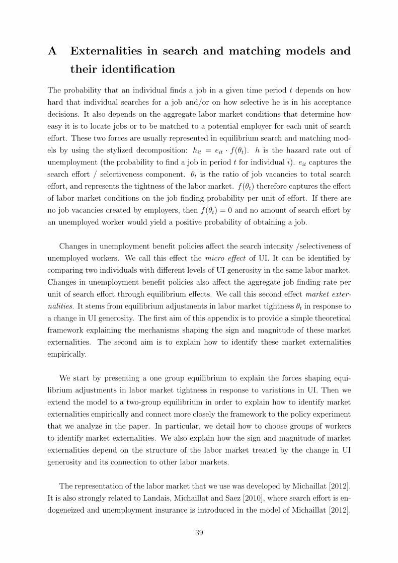
A Externalities in search and matching models and

their identification

The probability that an individual finds a job in a given time period t depends on how

hard that individual searches for a job and/or on how selective he is in his acceptance

decisions. It also depends on the aggregate labor market conditions that determine how

easy it is to locate jobs or to be matched to a potential employer for each unit of search

effort. These two forces are usually represented in equilibrium search and matching mod-

els by using the stylized decomposition: hit = eit · f(θt). h is the hazard rate out of

unemployment (the probability to find a job in period t for individual i). eit captures the

search effort / selectiveness component. θt is the ratio of job vacancies to total search

effort, and represents the tightness of the labor market. f(θt) therefore captures the effect

of labor market conditions on the job finding probability per unit of effort. If there are

no job vacancies created by employers, then f(θt) = 0 and no amount of search effort by

an unemployed worker would yield a positive probability of obtaining a job.

Changes in unemployment benefit policies affect the search intensity /selectiveness of

unemployed workers. We call this effect the micro effect of UI. It can be identified by

comparing two individuals with different levels of UI generosity in the same labor market.

Changes in unemployment benefit policies also affect the aggregate job finding rate per

unit of search effort through equilibrium effects. We call this second effect market exter-

nalities. It stems from equilibrium adjustments in labor market tightness θt in response to

a change in UI generosity. The first aim of this appendix is to provide a simple theoretical

framework explaining the mechanisms shaping the sign and magnitude of these market

externalities. The second aim is to explain how to identify these market externalities

empirically.

We start by presenting a one group equilibrium to explain the forces shaping equi-

librium adjustments in labor market tightness in response to variations in UI. Then we

extend the model to a two-group equilibrium in order to explain how to identify market

externalities empirically and connect more closely the framework to the policy experiment

that we analyze in the paper. In particular, we detail how to choose groups of workers

to identify market externalities. We also explain how the sign and magnitude of market

externalities depend on the structure of the labor market treated by the change in UI

generosity and its connection to other labor markets.

The representation of the labor market that we use was developed by Michaillat [2012].

It is also strongly related to Landais, Michaillat and Saez [2010], where search effort is en-

dogeneized and unemployment insurance is introduced in the model of Michaillat [2012].

39

Readers are referred to these two papers for further details on the set-up and equilibrium

analysis.

A.1 One group equilibrium

The labor market is characterized by the presence of matching frictions. We normalize the

size of labor force to unity. We present a simplified, static equilibrium analysis of search

and matching models and characterize the comparative static for steady state equilibria.

To keep things simple, we assume throughout that all workers within a group get the

same wage. We start by looking at a one group equilibrium, as in Landais, Michaillat

and Saez [2010], where all workers are eligible to the same unemployment benefits B, and

explain the two main mechanisms that shape the equilibrium response in labor market

tightness to a variation in unemployment benefits: the rat race effect (or labor demand

effect) and the wage effect.

Unemployed workers face v vacancies opened by firms, and the total number of matches

realized is given by an aggregate matching function m(e · u, v) = ωm · (e · u)η ·v1−η. Labor

market tightness θ = ve·u is defined as the ratio of vacancies to the aggregate search effort

in the labor market.

The individual job-finding probability is h = e · f(θ) = e ·m(1, θ), where e = e(B, θ) is

the optimal search effort of individuals given benefits and labor market tightness. Effort

is a decreasing function of unemployment benefits ∂e/∂B < 0. To further simplify the

presentation, we assume that ∂e∂θ

= 0. The assumption that the elasticity of job search

effort with respect to the job-finding rate is close to zero seems reasonable empirically.

As emphasized by Shimer [2004] labor market participation and other measures of search

intensity are, if anything, slightly countercyclical even after controlling for changing char-

acteristics of unemployed workers over the business cycle. The job-finding probability is

an increasing function of θ (f ′(θ) > 0). From the definition of the matching function

we can also define the vacancy-filling probability for each vacancy opened by the firm

q(θ) = m(1/θ, 1) which is a decreasing function of labor market tightness ∂q(θ)∂θ

< 0.

We denote by ns the probability that a worker is employed (and by u = 1 − ns the

corresponding unemployment probability). Using the steady state equality of flows in and

out of unemployment, we have that

ns =ef(θ)

λ+ ef(θ)(6)

40

where λ is the exogenous separation rate. Following Michaillat [2012], we interpret

ns = ns(θ, e(B)) as a labor supply that we can represent as an increasing function of

θ in a {n, θ} diagram.

A representative firm maximizes profit π = φ(n)−n ·w− rq(θ)·ψ ·n where φ(.) is total

output, n is employment and r is the recruiting cost of opening a vacancy. Firms take

labor market tightness as given, and for them it is equivalent to choose employment level

or the number of vacancies, given that v vacancies automatically translate into v · q(θ)job creations. The first-order condition of the firm with respect to employment level n is:

φ′(n) = w +rψ

q(θ)(7)

Equation (7) implicitly defines a labor demand function nd(θ, w) whose properties

depend in particular on the assumptions made on φ(.) and on the wage setting pro-

cess defining w. These properties are important to determine the sign and magnitude

of externalities, as explained below. In particular, note that when technology exhibits

diminishing returns to labor, with φ′(n) > 0 and φ′′(n) < 0, we have by implicit differen-

tiation of equation (7): ∂nd

∂θ< 0. So in this case, labor demand will be a downward sloping

function of θ as in Michaillat [2012]. The intuition for this negative relationship between

labor demand and labor market tightness is the following: as labor market tightness goes

up, the cost of opening vacancies goes up, as it takes longer to fill vacancies. Firms will

post fewer vacancies, bringing their level of employment down, which will increase labor

productivity and restore the profit from opening vacancies. It is also immediate to see

that when technology is linear and in the absence of aggregate demand effects, equation

(7) implicitly defines labor demand as a perfectly elastic function of labor market tightness.

Note also that, depending on the wage setting process, labor demand implicitly defined

by equation (7) can also be a function of unemployment benefits. If wages are bargained

over and workers have limited bargaining power, then wages will react to outside options

of workers and thus to variations in unemployment benefits B: w = w(B). As can be

seen from equation (7), an increase in B leading to a increase in wages w will, everything

else equal, decrease the net return from opening a vacancy and lead to a decrease in labor

demand nd.

We can now define a labor market equilibrium by the condition:

ns(θ, e(B)) = nd(θ, w(B)) (8)

Market externalities:

41

Equilibrium condition (8) defines θ as an endogenous variable, affected by the level

of benefits B of unemployed individuals in equilibrium. Because of this equilibrium ad-

justment of θ in response to a change in UI benefits, the effect of UI on the job finding

probability h = e · f(θ) can be decomposed into two parts, a micro-effect capturing the

change in search effort keeping labor market tightness constant and a “market external-

ity”, capturing the effect of the change in labor market tightness:

dh

dB=d(e · f(θ))

dB=

∂e

∂B· f(θ)︸ ︷︷ ︸

Micro effect

+

Market externality︷ ︸︸ ︷e · f ′(θ) · θ

B· εθB (9)

where εθB = dθdB

Bθ

is the elasticity of labor market tightness with respect to the generosity

of UI B. The second term on the right-hand side of equation (9) is the market externality,

which is defined as the variation in the job finding rate caused by equilibrium adjustments

in labor market tightness, keeping search effort constant.

The reason why we call this effect a “market externality” instead of a mere incidence

effect is because, as shown in Landais, Michaillat and Saez [2010], these equilibrium

adjustments in labor market tightness have first-order welfare effects when the Hosios

condition is not met.

Equilibrium adjustment of θ in response to a change in UI benefits ( dθdB

) is given by

fully differentiating equation (8).

dθ

dB=

∂nd

∂w∂w∂B− ∂ns

∂B∂ns

∂θ− ∂nd

∂θ

(10)

Equation (10) can also be rewritten in terms of elasticities:

εθB =εn

d

w · εwB − εns

B

εns

θ − εnd

θ

(11)

where the notation εXY refers to the elasticity of X w.r.t Y . From the previous equation,

we can now discuss the forces determining equilibrium adjustments of θ in response to a

change in benefits B. We focus in particular on two opposing forces: the rat-race effect

(or labor-demand effect), and the wage effect.

Rate race effect

The rate race effect is determined by the elasticity of labor-demand (εnd

θ ). If labor

demand is downward sloping (εnd

θ < 0) then the denominator in (11) is positive. Given

42

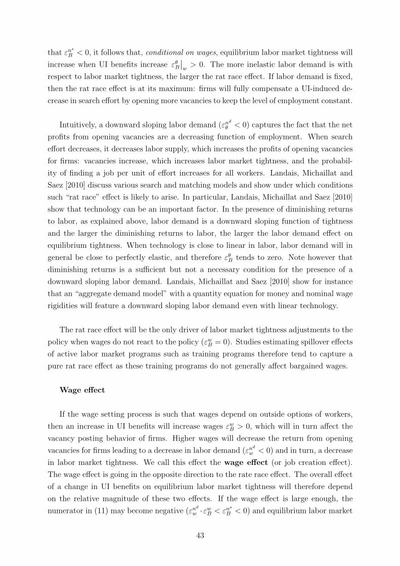
that εns

B < 0, it follows that, conditional on wages, equilibrium labor market tightness will

increase when UI benefits increase εθB∣∣w> 0. The more inelastic labor demand is with

respect to labor market tightness, the larger the rat race effect. If labor demand is fixed,

then the rat race effect is at its maximum: firms will fully compensate a UI-induced de-

crease in search effort by opening more vacancies to keep the level of employment constant.

Intuitively, a downward sloping labor demand (εnd

θ < 0) captures the fact that the net

profits from opening vacancies are a decreasing function of employment. When search

effort decreases, it decreases labor supply, which increases the profits of opening vacancies

for firms: vacancies increase, which increases labor market tightness, and the probabil-

ity of finding a job per unit of effort increases for all workers. Landais, Michaillat and

Saez [2010] discuss various search and matching models and show under which conditions

such “rat race” effect is likely to arise. In particular, Landais, Michaillat and Saez [2010]

show that technology can be an important factor. In the presence of diminishing returns

to labor, as explained above, labor demand is a downward sloping function of tightness

and the larger the diminishing returns to labor, the larger the labor demand effect on

equilibrium tightness. When technology is close to linear in labor, labor demand will in

general be close to perfectly elastic, and therefore εθB tends to zero. Note however that

diminishing returns is a sufficient but not a necessary condition for the presence of a

downward sloping labor demand. Landais, Michaillat and Saez [2010] show for instance

that an “aggregate demand model” with a quantity equation for money and nominal wage

rigidities will feature a downward sloping labor demand even with linear technology.

The rat race effect will be the only driver of labor market tightness adjustments to the

policy when wages do not react to the policy (εwB = 0). Studies estimating spillover effects

of active labor market programs such as training programs therefore tend to capture a

pure rat race effect as these training programs do not generally affect bargained wages.

Wage effect

If the wage setting process is such that wages depend on outside options of workers,

then an increase in UI benefits will increase wages εwB > 0, which will in turn affect the

vacancy posting behavior of firms. Higher wages will decrease the return from opening

vacancies for firms leading to a decrease in labor demand (εnd

w < 0) and in turn, a decrease

in labor market tightness. We call this effect the wage effect (or job creation effect).

The wage effect is going in the opposite direction to the rate race effect. The overall effect

of a change in UI benefits on equilibrium labor market tightness will therefore depend

on the relative magnitude of these two effects. If the wage effect is large enough, the

numerator in (11) may become negative (εnd

w ·εwB < εns

B < 0) and equilibrium labor market

43

tightness will decrease in response to an increase in benefits. If the wage effect is small in

magnitude, then the rat race effect will dominate: the numerator in (11) will be positive

(εns

B < εnd

w · εwB < 0) and labor market tightness will increase in response to an increase in

UI benefits.

A.2 Identification of market externalities in a two group equi-

librium

Identification of the micro effect in equation (9) is relatively straightforward. The ideal

experiment is to offer higher unemployment benefits to a randomly selected and small

subset of individuals within a labor market and compare unemployment durations be-

tween these treated individuals and the other jobseekers. In practice, the micro effect is

estimated by comparing individuals with different benefits in the same labor market at a

given time, while controlling for individual characteristics.

Identification of market externalities in equation (9) is more complicated, in large part

due to the lack of good measures of labor market tightness.22 We show here how one can

use labor market outcomes of different group of workers in the same labor market to iden-

tify market externalities of UI benefits. We introduce two groups of workers a and b and

assume there are p workers of group a who are eligible to unemployment benefits Ba and

1−p workers workers of group b who are eligible to unemployment benefit Bb. The group

shares p and 1− p are exogenously given. We start from a situation where Ba = Bb and

look at the effect on the steady state equilibrium of an increase in benefits for workers of

group a: dBa > 0.

We denote by nsa (resp. nsb) the probability that a worker of group a (resp. b) is

employed (and by ua = 1 − nsa the corresponding unemployment probability) There are

u = ua + ub unemployed workers. When unemployed, each individual worker exerts some

effort ei = e(Bi), i = (a, b), where e is a decreasing function of benefits received B.

Workers of both groups are assumed to be in the same labor market and we define a

labor market as the place where workers compete for the same job vacancies.

A labor market is therefore characterized by a unique labor market tightness in equilib-

rium, and matching is random between identical job vacancies posted by firms and all the

22A notable exception is Marinescu [2014] who uses very detailed information on vacancies and jobapplications from CareerBuilder.com, the largest American online job board, to compute the effects ofUI extensions on aggregate search effort (e · u) measured by job applications and on vacancy posting (v)at the state level. She finds a negative effect of UI extensions on job applications but no effect of UIextensions on vacancy posting. Since θ = v/(e · u), these results imply that more generous UI benefitsincrease labor market tightness.

44

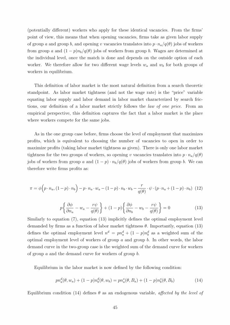
(potentially different) workers who apply for these identical vacancies. From the firms’

point of view, this means that when opening vacancies, firms take as given labor supply

of group a and group b, and opening v vacancies translates into p ·na/q(θ) jobs of workers

from group a and (1− p)nb/q(θ) jobs of workers from group b. Wages are determined at

the individual level, once the match is done and depends on the outside option of each

worker. We therefore allow for two different wage levels wa and wb for both groups of

workers in equilibrium.

This definition of labor market is the most natural definition from a search theoretic

standpoint. As labor market tightness (and not the wage rate) is the “price” variable

equating labor supply and labor demand in labor market characterized by search fric-

tions, our definition of a labor market strictly follows the law of one price. From an

empirical perspective, this definition captures the fact that a labor market is the place

where workers compete for the same jobs.

As in the one group case before, firms choose the level of employment that maximizes

profits, which is equivalent to choosing the number of vacancies to open in order to

maximize profits (taking labor market tightness as given). There is only one labor market

tightness for the two groups of workers, so opening v vacancies translates into p · na/q(θ)jobs of workers from group a and (1− p) · nb/q(θ) jobs of workers from group b. We can

therefore write firms profits as:

π = φ(p ·na, (1−p) ·nb

)−p ·na ·wa− (1−p) ·nb ·wb−

r

q(θ)·ψ · (p ·na + (1−p) ·nb) (12)

p

{∂φ

∂na− wa −

rψ

q(θ)

}+ (1− p)

{∂φ

∂nb− wb −

rψ

q(θ)

}= 0 (13)

Similarly to equation (7), equation (13) implicitly defines the optimal employment level

demanded by firms as a function of labor market tightness θ. Importantly, equation (13)

defines the optimal employment level nd = pnda + (1 − p)ndb as a weighted sum of the

optimal employment level of workers of group a and group b. In other words, the labor

demand curve in the two-group case is the weighted sum of the demand curve for workers

of group a and the demand curve for workers of group b.

Equilibrium in the labor market is now defined by the following condition:

pnda(θ, wa) + (1− p)ndb(θ, wb) = pnsa(θ, Ba) + (1− p)nsb(θ, Bb) (14)

Equilibrium condition (14) defines θ as an endogenous variable, affected by the level of

45

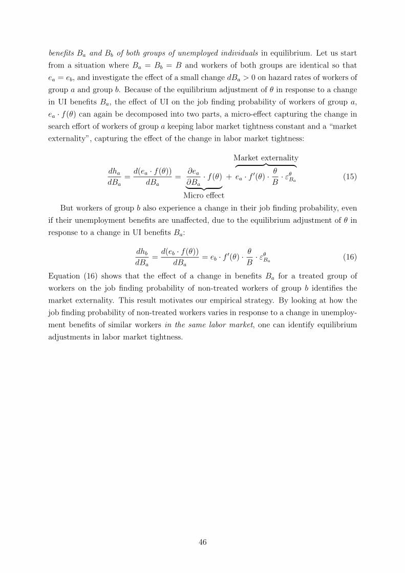
benefits Ba and Bb of both groups of unemployed individuals in equilibrium. Let us start

from a situation where Ba = Bb = B and workers of both groups are identical so that

ea = eb, and investigate the effect of a small change dBa > 0 on hazard rates of workers of

group a and group b. Because of the equilibrium adjustment of θ in response to a change

in UI benefits Ba, the effect of UI on the job finding probability of workers of group a,

ea · f(θ) can again be decomposed into two parts, a micro-effect capturing the change in

search effort of workers of group a keeping labor market tightness constant and a “market

externality”, capturing the effect of the change in labor market tightness:

dhadBa

=d(ea · f(θ))

dBa

=∂ea∂Ba

· f(θ)︸ ︷︷ ︸Micro effect

+

Market externality︷ ︸︸ ︷ea · f ′(θ) ·

θ

B· εθBa (15)

But workers of group b also experience a change in their job finding probability, even

if their unemployment benefits are unaffected, due to the equilibrium adjustment of θ in

response to a change in UI benefits Ba:

dhbdBa

=d(eb · f(θ))

dBa

= eb · f ′(θ) ·θ

B· εθBa (16)

Equation (16) shows that the effect of a change in benefits Ba for a treated group of

workers on the job finding probability of non-treated workers of group b identifies the

market externality. This result motivates our empirical strategy. By looking at how the

job finding probability of non-treated workers varies in response to a change in unemploy-

ment benefits of similar workers in the same labor market, one can identify equilibrium

adjustments in labor market tightness.

46

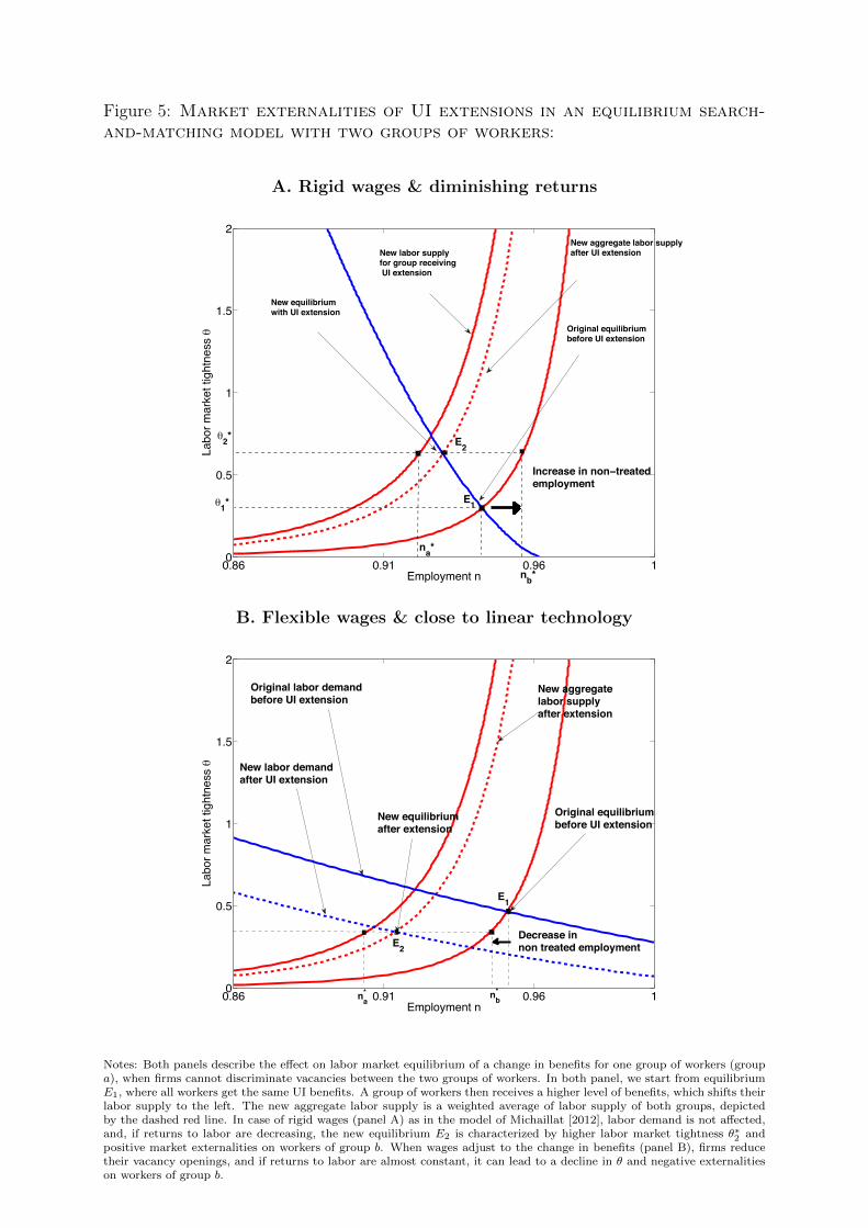
Figure 5: Market externalities of UI extensions in an equilibrium search-and-matching model with two groups of workers:

A. Rigid wages & diminishing returns

0.86 0.91 0.96 10

0.5

1

1.5

2

Employment n

Labo

r mar

ket t

ight

ness

e Original equilibriumbefore UI extension

e2*

e1*

New equilibriumwith UI extension

New labor supplyfor group receiving UI extension

New aggregate labor supplyafter UI extension

Increase in non−treatedemployment

E2

E1

na*

nb*

B. Flexible wages & close to linear technology

0.86 0.91 0.96 10

0.5

1

1.5

2

Employment n

Labo

r mar

ket t

ight

ness

e

Decrease in non treated employment

E1

E2

nb*na

*

New labor demandafter UI extension

Original labor demandbefore UI extension

New aggregate labor supply after extension

Original equilibriumbefore UI extension

New equilibriumafter extension

Notes: Both panels describe the effect on labor market equilibrium of a change in benefits for one group of workers (groupa), when firms cannot discriminate vacancies between the two groups of workers. In both panel, we start from equilibriumE1, where all workers get the same UI benefits. A group of workers then receives a higher level of benefits, which shifts theirlabor supply to the left. The new aggregate labor supply is a weighted average of labor supply of both groups, depictedby the dashed red line. In case of rigid wages (panel A) as in the model of Michaillat [2012], labor demand is not affected,and, if returns to labor are decreasing, the new equilibrium E2 is characterized by higher labor market tightness θ∗2 andpositive market externalities on workers of group b. When wages adjust to the change in benefits (panel B), firms reducetheir vacancy openings, and if returns to labor are almost constant, it can lead to a decline in θ and negative externalitieson workers of group b.

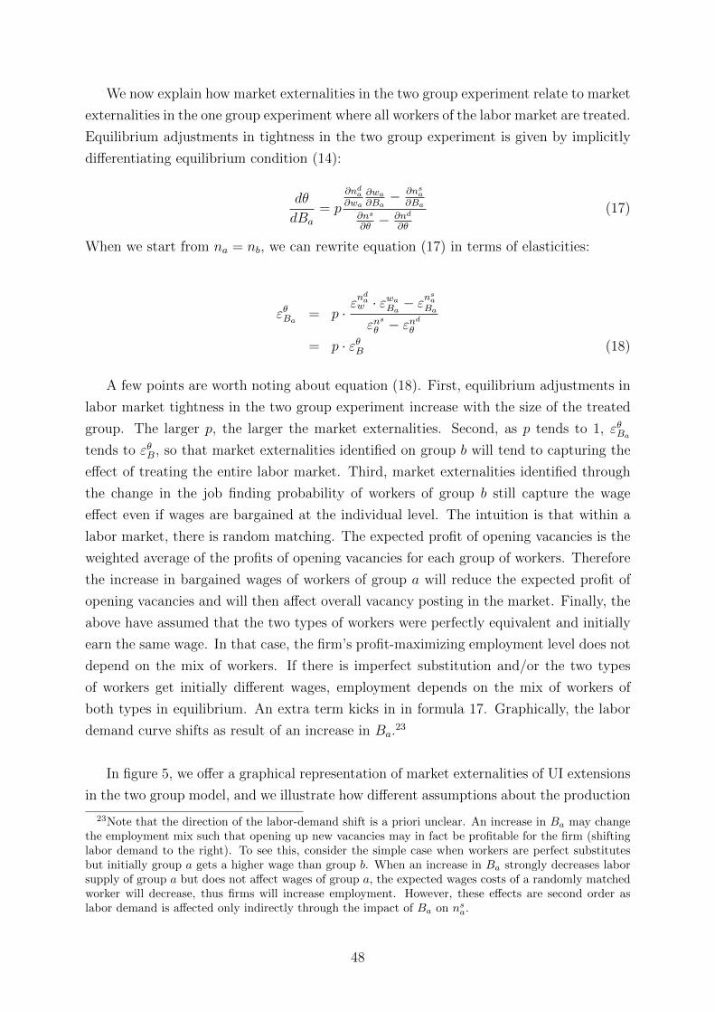
We now explain how market externalities in the two group experiment relate to market

externalities in the one group experiment where all workers of the labor market are treated.

Equilibrium adjustments in tightness in the two group experiment is given by implicitly

differentiating equilibrium condition (14):

dθ

dBa

= p

∂nda∂wa

∂wa∂Ba− ∂nsa

∂Ba∂ns

∂θ− ∂nd

∂θ

(17)

When we start from na = nb, we can rewrite equation (17) in terms of elasticities:

εθBa = p ·εndaw · εwaBa − ε

nsaBa

εns

θ − εnd

θ

= p · εθB (18)

A few points are worth noting about equation (18). First, equilibrium adjustments in

labor market tightness in the two group experiment increase with the size of the treated

group. The larger p, the larger the market externalities. Second, as p tends to 1, εθBatends to εθB, so that market externalities identified on group b will tend to capturing the

effect of treating the entire labor market. Third, market externalities identified through

the change in the job finding probability of workers of group b still capture the wage

effect even if wages are bargained at the individual level. The intuition is that within a

labor market, there is random matching. The expected profit of opening vacancies is the

weighted average of the profits of opening vacancies for each group of workers. Therefore

the increase in bargained wages of workers of group a will reduce the expected profit of

opening vacancies and will then affect overall vacancy posting in the market. Finally, the

above have assumed that the two types of workers were perfectly equivalent and initially

earn the same wage. In that case, the firm’s profit-maximizing employment level does not

depend on the mix of workers. If there is imperfect substitution and/or the two types

of workers get initially different wages, employment depends on the mix of workers of

both types in equilibrium. An extra term kicks in in formula 17. Graphically, the labor

demand curve shifts as result of an increase in Ba.23

In figure 5, we offer a graphical representation of market externalities of UI extensions

in the two group model, and we illustrate how different assumptions about the production

23Note that the direction of the labor-demand shift is a priori unclear. An increase in Ba may changethe employment mix such that opening up new vacancies may in fact be profitable for the firm (shiftinglabor demand to the right). To see this, consider the simple case when workers are perfect substitutesbut initially group a gets a higher wage than group b. When an increase in Ba strongly decreases laborsupply of group a but does not affect wages of group a, the expected wages costs of a randomly matchedworker will decrease, thus firms will increase employment. However, these effects are second order aslabor demand is affected only indirectly through the impact of Ba on nsa.

48

function and the wage setting process affect the sign and magnitude of externalities. Both

panels describe the effect on labor market equilibrium of a change in benefits for one group

of workers (group a), when firms cannot discriminate vacancies between the two groups

of workers. In both panel, we start from equilibrium E1, where all workers get the same

UI benefits. Workers of group a then receive a higher level of benefits, which shifts their

labor supply to the left. The new aggregate labor supply is a weighted average of labor

supply of both groups, depicted by the dashed red line. In case of rigid wages (panel A) as

in the model of Michaillat [2012], labor demand is not affected, and, if returns to labor are

decreasing, the new equilibrium E2 is characterized by higher labor market tightness θ∗2

and positive market externalities on workers of group b. When wages adjust to the change

in benefits (panel B), firms reduce their vacancy openings, and if returns to labor are al-

most constant, it can lead to a decline in θ and negative externalities on workers of group b.

Implications for the wedge between micro and macro effects of UI

We are interested in recovering from the two group experiment, the wedge between

micro and macro effects of treating the whole labor market. More specifically, starting

from equation (9), we are interested in the wedge W = 1 − eM/em where eM = dhdB

is

the total effect on job finding rate of treating the whole market by an increase dB in UI

benefits (“macro effect”) and em is the “micro effect” from equation (9) (i.e. the effect of

an increase dB in UI benefits on individual job finding rate).

From equation (9) we know that W = eX

em, where eX = e · f ′(θ) · θ

B· εθB is the market

externality of treating the whole labor market. From equations (16) and (18), we know

that in the two group experiments, starting from a situation where both groups have the

same benefits and search effortdhbdBa

= p · eX (19)

In other words, the effect of changing benefits for workers of group a on the job finding

rates of workers of group b identifies p times the externality of treating all workers, where

p is the fraction of workers of group a in the labor market.

In the two group experiment, again starting from a situation where both groups have

the same benefits and search effort, we also know that the micro effect em will be the

same than when treating the whole market. This means that the micro effect ∂e∂B· f(θ)

from equation (9) is equal to the micro effect from equation (15): ∂ea∂Ba· f(θ). And from

equations (15) and (16), we know that the micro effect will be identified in the two group

experiment as

em =dhadBa

− dhbdBa

(20)

49

In other words, the micro effect is identified by the effect of the change in UI benefits

on the job finding rate of workers of group a minus the effect on the job finding rate of

workers of group b. It follows from equations (19) and (20) that we can identify the wedge

W of treating the whole market in the two group experiment:

W =1

p·

dhbdBa

dhadBa− dhb

dBa

(21)

Using the fact that we start from a situation where Ba = Bb and ha = hb, and under

the approximation that hazard rates are somewhat constant over a spell so that the

duration of unemployment D ≈ 1/h we can rewrite equation 21 in terms of responses of

unemployment duration:

W =1

p·

dDbdBa

dDadBa− dDb

dBa

(22)

A.3 Market externalities across labor markets

In most quasi-experiments involving variations in the generosity of unemployment ben-

efits, treatment is restricted to some but not all labor markets. The REBP program is

no exception. The program extended the duration of UI benefits for individuals above

age 50 in specific regions meeting specific criteria. A firms can adjust to the policy not

only by changing the number of vacancy it opens in the treated labor market, but also by

changing the number of vacancies it opens in other labor markets where there exists close

substitutes to the treated population. In other words, there exist “non-treated” labor

markets that, due to their (geographic or technological) proximity to the treated labor

market, will also be affected by the policy in equilibrium. We show here how the existence

of other labor markets will affect market externalities. First, we show how (and discuss

why) equilibrium labor market conditions in other markets will be affected. Then, we

discuss how the existence of other markets affect the magnitude of market externalities

in the treated market.

How are other labor markets affected by a change in UI policy in one labor market?

We focus again on a two group model, but now group a and group b are assumed to be in

two different labor markets. This means that firms can perfectly discriminate between the

two groups of workers when they open vacancies. In practice, there will be vacancies va to

which only workers of group a will apply and vacancies vb to which only workers of group

b will apply. The ability of firms to direct their search by tailoring the characteristics of

vacancies to each group of workers means that there will be in effect two labor markets

50

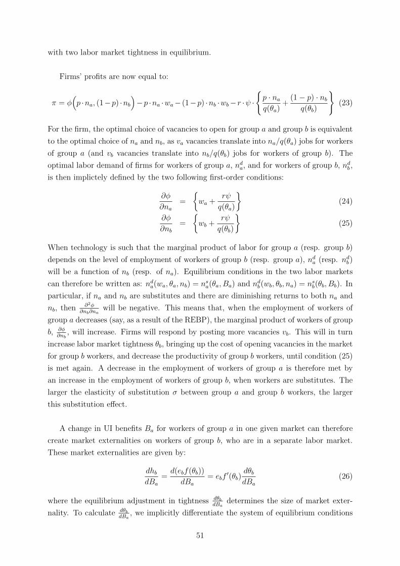
with two labor market tightness in equilibrium.

Firms’ profits are now equal to:

π = φ(p ·na, (1−p) ·nb

)−p ·na ·wa− (1−p) ·nb ·wb− r ·ψ ·

{p · naq(θa)

+(1− p) · nb

q(θb)

}(23)

For the firm, the optimal choice of vacancies to open for group a and group b is equivalent

to the optimal choice of na and nb, as va vacancies translate into na/q(θa) jobs for workers

of group a (and vb vacancies translate into nb/q(θb) jobs for workers of group b). The

optimal labor demand of firms for workers of group a, nda, and for workers of group b, ndb ,

is then implictely defined by the two following first-order conditions:

∂φ

∂na=

{wa +

rψ

q(θa)

}(24)

∂φ

∂nb=

{wb +

rψ

q(θb)

}(25)

When technology is such that the marginal product of labor for group a (resp. group b)

depends on the level of employment of workers of group b (resp. group a), nda (resp. ndb)

will be a function of nb (resp. of na). Equilibrium conditions in the two labor markets

can therefore be written as: nda(wa, θa, nb) = nsa(θa, Ba) and ndb(wb, θb, na) = nsb(θb, Bb). In

particular, if na and nb are substitutes and there are diminishing returns to both na and

nb, then ∂2φ∂nb∂na

will be negative. This means that, when the employment of workers of

group a decreases (say, as a result of the REBP), the marginal product of workers of group

b, ∂φ∂nb

, will increase. Firms will respond by posting more vacancies vb. This will in turn

increase labor market tightness θb, bringing up the cost of opening vacancies in the market

for group b workers, and decrease the productivity of group b workers, until condition (25)

is met again. A decrease in the employment of workers of group a is therefore met by

an increase in the employment of workers of group b, when workers are substitutes. The

larger the elasticity of substitution σ between group a and group b workers, the larger

this substitution effect.

A change in UI benefits Ba for workers of group a in one given market can therefore

create market externalities on workers of group b, who are in a separate labor market.

These market externalities are given by:

dhbdBa

=d(ebf(θb))

dBa

= ebf′(θb)

dθbdBa

(26)

where the equilibrium adjustment in tightness dθbdBa

determines the size of market exter-

nality. To calculate dθbdBa

, we implicitly differentiate the system of equilibrium conditions

51

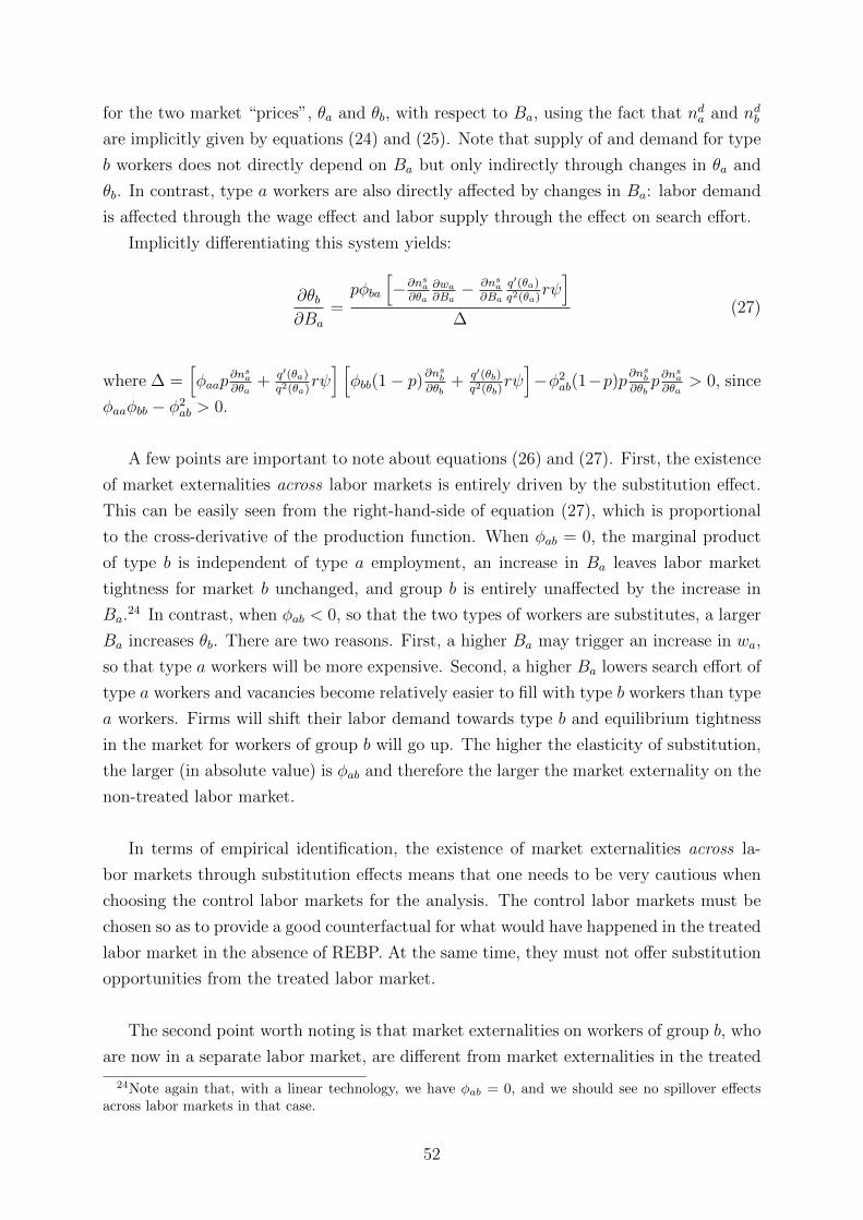
for the two market “prices”, θa and θb, with respect to Ba, using the fact that nda and ndbare implicitly given by equations (24) and (25). Note that supply of and demand for type

b workers does not directly depend on Ba but only indirectly through changes in θa and

θb. In contrast, type a workers are also directly affected by changes in Ba: labor demand

is affected through the wage effect and labor supply through the effect on search effort.

Implicitly differentiating this system yields:

∂θb∂Ba

=pφba

[−∂nsa

∂θa∂wa∂Ba− ∂nsa

∂Ba

q′(θa)q2(θa)

rψ]

∆(27)

where ∆ =[φaap

∂nsa∂θa

+ q′(θa)q2(θa)

rψ] [φbb(1− p)

∂nsb∂θb

+ q′(θb)q2(θb)

rψ]−φ2

ab(1−p)p∂nsb∂θbp∂n

sa

∂θa> 0, since

φaaφbb − φ2ab > 0.

A few points are important to note about equations (26) and (27). First, the existence

of market externalities across labor markets is entirely driven by the substitution effect.

This can be easily seen from the right-hand-side of equation (27), which is proportional

to the cross-derivative of the production function. When φab = 0, the marginal product

of type b is independent of type a employment, an increase in Ba leaves labor market

tightness for market b unchanged, and group b is entirely unaffected by the increase in

Ba.24 In contrast, when φab < 0, so that the two types of workers are substitutes, a larger

Ba increases θb. There are two reasons. First, a higher Ba may trigger an increase in wa,

so that type a workers will be more expensive. Second, a higher Ba lowers search effort of

type a workers and vacancies become relatively easier to fill with type b workers than type

a workers. Firms will shift their labor demand towards type b and equilibrium tightness

in the market for workers of group b will go up. The higher the elasticity of substitution,

the larger (in absolute value) is φab and therefore the larger the market externality on the

non-treated labor market.

In terms of empirical identification, the existence of market externalities across la-

bor markets through substitution effects means that one needs to be very cautious when

choosing the control labor markets for the analysis. The control labor markets must be

chosen so as to provide a good counterfactual for what would have happened in the treated

labor market in the absence of REBP. At the same time, they must not offer substitution

opportunities from the treated labor market.

The second point worth noting is that market externalities on workers of group b, who

are now in a separate labor market, are different from market externalities in the treated

24Note again that, with a linear technology, we have φab = 0, and we should see no spillover effectsacross labor markets in that case.

52

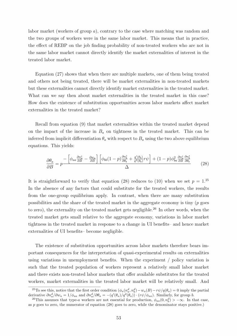
labor market (workers of group a), contrary to the case where matching was random and

the two groups of workers were in the same labor market. This means that in practice,

the effect of REBP on the job finding probability of non-treated workers who are not in

the same labor market cannot directly identify the market externalities of interest in the

treated labor market.

Equation (27) shows that when there are multiple markets, one of them being treated

and others not being treated, there will be market externalities in non-treated markets

but these externalities cannot directly identify market externalities in the treated market.

What can we say then about market externalities in the treated market in this case?

How does the existence of substitution opportunities across labor markets affect market

externalities in the treated market?

Recall from equation (9) that market externalities within the treated market depend

on the impact of the increase in Ba on tightness in the treated market. This can be

inferred from implicit differentiation θa with respect to Ba using the two above equilibrium

equations. This yields:

∂θa∂B

= p−[φaa

∂nsa∂B− ∂wa

∂B

] [φbb(1− p)

∂nsb∂θb

+ q′(θb)q2(θb)

rψ]

+ (1− p)φ2ba∂nsa∂B

∂nsb∂θb

∆(28)

It is straightforward to verify that equation (28) reduces to (10) when we set p = 1.25

In the absence of any factors that could substitute for the treated workers, the results

from the one-group equilibrium apply. In contrast, when there are many substitution

possibilities and the share of the treated market in the aggregate economy is tiny (p goes

to zero), the externality on the treated market gets negligible.26 In other words, when the

treated market gets small relative to the aggregate economy, variations in labor market

tightness in the treated market in response to a change in UI benefits– and hence market

externalities of UI benefits– become negligible.

The existence of substitution opportunities across labor markets therefore bears im-

portant consequences for the interpretation of quasi-experimental results on externalities

using variations in unemployment benefits. When the experiment / policy variation is

such that the treated population of workers represent a relatively small labor market

and there exists non-treated labor markets that offer available substitutes for the treated

workers, market externalities in the treated labor market will be relatively small. And

25To see this, notice that the first order condition (φa(nda, ndb)−wa(B)−rψ/q(θa) = 0 imply the partial

derivative ∂nda/∂wa = 1/φaa and ∂nda/∂θa = −(q′(θa)/q2(θa)) · (rψ/φaa). Similarly, for group b.26This assumes that type-a workers are not essential for production, φaa(0, ndb) > −∞. In that case,

as p goes to zero, the numerator of equation (28) goes to zero, while the denominator stays positive.)

53

estimated equilibrium adjustments in labor market tightness in such a context should

be interpreted as a clear lower bound on the equilibrium adjustments in labor market

tightness that would occur if the whole population of workers were to be treated.

A.4 Endogenous layoffs

The separation rate λ as been assumed exogenous. But in practice λ might be endoge-

nous to UI benefits (λ = λ(B)) and there is indeed evidence that the separation rate

increased for eligible workers during the REBP period (Winter-Ebmer [1996]), implying

that ∂λa/∂(Ba) > 0. How will the response of the separation rate to UI benefits af-

fect market externalities of UI? From the definition of labor supply given in equation 6,

ns = ef(θ)λ+ef(θ)

, which follows from the equality of flows in and out of unemployment in

the steady-state, it appears clearly that an increase in the separation rate λ will shift

labor supply downwards everything else equal. For a given search effort level, and for a

given labor market tightness, an increase in the separation rate means that the stock of

unemployed will be larger in the steady state and therefore the probability of finding a

job (ns) will be lower. An increase in the separation rate is equivalent to a downward

shift in labor supply and its effect on labor supply is comparable to that of a decrease in

search effort. If both search effort and the separation rate are responsive to UI benefits,

the effect of a change in benefit of workers of group a on labor supply of group a is the

sum of a search effort effect (e′a · λa) and of a separation rate effect (ea · λ′a):

∂nsa∂Ba

=[e′a · λa − ea · λ′a]f(θ)

(λa + eaf(θ))2

In the context of REBP, because the separation rate effect ea · λ′a > 0 is significantly

positive, the downward shift in labor supply of treated workers will be even stronger than

if only search effort had reacted to the policy.

But an increase in the separation rate λ also increases recruiting costs of firms. As

new jobs have a higher probability of being terminated, the net present value of a job

decreases. This will create a downward shift of nd that can easily be seen in equation

(7) which implicitly determines labor demand of firms nd as a decreasing function of the

layoff rate: ∂nd/∂λ ≤ 0. So the overall effect on labor market tightness of a change in

benefits for workers of group a when layoffs are endogenous is:

dθ

dBa

= p

∂nda∂wa

∂wa∂Ba

+ ∂nda∂λa

∂λa∂Ba− ∂nsa

∂Ba∂ns

∂θ− ∂nd

∂θ

(29)

where ∂nda∂λa

∂λa∂Ba

is the layoff rate effect on labor demand. The overall effect of endogenous

54

layoffs on equilibrium adjustments in labor market tightness dθdBa

is therefore ambiguous,

as can be seen by comparing equation (29) to equation (17). The presence of endogenous

layoffs creates a negative layoff rate effect on labor demand ( ∂nda∂λa

∂λa∂Ba≤ 0), which will

tend to reduce labor market tightness, but it also increases the magnitude of the shift in

labor supply ∂nsa∂Ba

as discussed earlier, which will tend to increase labor market tightness.

The relative magnitude of these two effects will therefore determine if endogenous layoffs

deepens or attenuates the effect of UI on equilibrium labor market tightness.

B Defining labor markets using vacancy data

Identifying which workers are competing for the same vacancies workers satisfying the

REBP-eligibility requirements is critical to determine and define the relevant labor mar-

kets that are affected by externalities of the REBP program. As explained in section A.2,

when treated and non-treated workers are in the same labor market, i.e. competing for

the same vacancies, the effect of the program on non-treated workers can identify equilib-

rium labor market tightness in the labor market. When treated and non-treated workers

are competing for different vacancies, there are in practice two search markets for labor,

and the effect of the program on non-treated workers cannot directly identify equilibrium

adjustments in the treated market.

To determine which workers are competing for the same vacancies as REBP eligible

workers, we use detailed micro data on the universe of job vacancies posted in public

employment agencies available for the period 1994-1998. (Vacancies posted in public em-

ployment agencies represent 30% to 40% of all posted vacancies). This data set has two

important features. First, the data records for each vacancy all the detailed information

about the characteristics of the vacancy. This includes the firm identifier of the firm post-

ing the vacancy, the date (in month) at which the vacancy is opened and the date at which

it is closed, the reason for closing the vacancy (the vacancy has been filled, search has

been abandoned, etc.), the identifier of the public employment service where the vacancy

is posted, the industry and job classifications of the job, details on the duration and type

of the contract (full-time,/part-time tenured/non-tenured, seasonal job, etc.), the age re-

quirement if any, the education requirement if any, the gender requirement if any, and the

posted wage or range of wage if any. Second, the data contains the personal identifier of

the person who filled the vacancy if the vacancy is filled. This personal identifier enables

us to match this vacancy data to the ASSD and determine the characteristics and REBP

eligibility status of the person filling the vacancy.

Our strategy consists in using all the information that we have on each vacancy, and

55

estimate how well the characteristics of each vacancy predicts the REBP eligibility status

of the worker who fills the vacancy. If there is perfect discrimination in vacancies between

eligible and non-eligible workers, then eligible and non-eligible workers will be competing

for two different sets of vacancies and will effectively be in two different labor markets

from a search-theoretic perspective. Empirically, this means that characteristics of va-

cancies for eligible and non-eligible workers are different, and therefore characteristics of

vacancies should predict very well whether the individual filling the vacancy is eligible to

REBP or not. To the contrary, if eligible and non-eligible workers are in the same job-

search market, they will compete for the same vacancies. When opening a vacancy in this

market, and conditional on search effort of eligible and non-eligible workers, a firm will be

randomly matched to an eligible or to a non-eligible worker. In other words, conditional

on search effort of eligible and non-eligible workers, matching is random across eligible

and non-eligible workers and vacancies in this market will be filled (randomly) by eligible

or non-eligible workers. In this case, the characteristics of a vacancy will have very little

predictive power on the eligibility status of the worker who fills it.

To implement this strategy, we take all vacancies opened by firms located in REBP

regions that ended up being filled (by REBP eligible or non-eligible male workers) during

1994 to 1998. (Before this period, the quality of the data is too weak and thus cannot be

used for our analysis.) We estimate the following latent variable model:

Y ∗i = X ′iβ + εi

Yi =

{0 if Y ∗i < 0

1 if Y ∗i ≥ 0

where Yi is a dummy variable indicating whether the worker filling vacancy i is eligible

to REBP or not, and Xi is a vector of all the characteristics of vacancy i. These char-

acteristics are the two-digit industry code of the firm opening the vacancy, the two-digit

occupation code of the job, the duration of the contract (temporary contract, unlimited

contract, seasonal job, holiday work, etc.), whether the job is full-time, part-time or flex-

ible hours, whether the job hours are negotiable or not, whether the job implies shift

work, whether it implies night or extra hours work, whether the job is an apprenticeship,

the size of the firm (in 5 categories), the age required for the job if any, and the level of

education required for the job (in 17 categories) if any. We estimate this model using a

logit. We run the model separately for various categories of non-eligible workers (35 to 40

years old workers, 40 to 45 years old workers, 45 to 50 years old workers, and 50-54 years

old non-eligible workers) in order to compare each of these categories of workers to REBP

eligible workers. For each of the categories of non-eligible workers, we then analyze the

predictive power of the model using various goodness-of-fit measures.

56

In figure 1 panel A, we start by plotting the p-value of two standard goodness-of-fit

tests for the logit model, the Pearson’s χ2 goodness of fit test and the Hosmer-Lemeshow

χ2 goodness of fit test, for different categories of non-eligible workers. A low p-value for

the test indicates a poor fit of the data. Both tests suggest that the model fits the data

very well for comparing eligible workers to non-eligible workers aged 35 to 40, but tend

to perform more and more poorly as we use non-eligible workers that are older. When

comparing eligible workers to non-eligible workers aged 50 to 54, the p-value is very close

to zero, and the goodness-of-fit of the model is extremely poor. This suggests that the

predictive power of vacancy characteristics on eligibility is very good when comparing

workers that are below 50 to eligible workers, but very low when comparing eligible and

non-eligible workers aged 50 to 54. In other words, workers age below 50 seem to fill

vacancies that have characteristics that are very different from the vacancies filled by

eligible workers. But eligible and non-eligible workers above 50 seem to fill vacancies that

have very similar characteristics. This suggests that workers aged below 50 are likely to

be in a different job search market than eligible workers, but non-eligible workers aged 50

to 54 are very likely to compete for the same vacancies as eligible workers.

In panel B of figure 1, we plot the fraction of observations that are incorrectly pre-

dicted by the model (i.e. the predicted eligibility status to REBP is different from the

true eligibility status of the worker filling the vacancy) for all categories of non-eligible

workers. The fraction of misclassified observations is less than 7.5% for the model com-

paring eligible workers to non-eligible workers aged 30 to 40, but increases up to more

than 25% for the model comparing eligible workers to non-eligible workers aged 50 to to

54. We also plot the fraction of type I errors, i.e. the fraction of true non-eligible workers

that are predicted as being eligible to REBP by the model. Type I errors are particularly

relevant in our context. They provide information about how likely it is that a non-eligible

worker is competing for a vacancy that has been “tailored” to eligible workers based on its

characteristics. In this sense, type I errors provide direct information about the intensity

of the competition that eligible workers receive from various groups of non-eligible work-

ers when a vacancy is opened in “their” search market. The figure indicates that type

I errors seem to be particularly severe when comparing eligible workers to non-eligible

workers aged 50 to 54. Because classification is sensitive to the relative sizes of each

component group, and always favors classification into the larger group, the classification

error measures of panel B should still be interpreted with caution. We therefore tend to

prefer goodness-of-fit measures presented in panel A.

These results help inform our identification strategy and choose the proper groups of

non-eligible workers to identify the presence of externalities. The results indicate that it

57

is much more likely for non-eligible workers aged 50 and over to compete for the same

vacancies as eligible workers than for non-eligible workers aged below 50. This means that

non-eligible workers aged 50 and above are likely to be in the same job-search market as

eligible workers, while non-eligible workers aged below 50 tend to compete for different

vacancies and are therefore in a different job-search market. This means that the effect

of REBP on job-finding probabilities of eligible workers aged 50 and above is more likely

to identify variations in labor market tightness in the job-search market of REBP-treated

workers. As explained in section A.2, these variations in labor market tightness in the

job-search market of REBP-treated workers capture both the rat race effect and the wage

effect of UI, and are the relevant variations to consider to identify the equilibrium effect

of variations in UI in a given labor market.

Non-eligible workers below 50 years old, to the contrary, seem to be competing for dif-

ferent vacancies than workers eligible to REBP. This means that they are more likely to

operate in a different search market than workers eligible to REBP. The effect of REBP on

their job finding probability is therefore more likely to identify externalities across search

markets. In section A.3, we have shown that such externalities stem from substitution

effects, and cannot directly identify the effect of REBP on the labor market tightness in

the search market of treated workers.

Overall, the vacancy data is useful to determine the scope of the different job search

markets. This analysis indicates that the externalities that we may find on non-eligible

workers may be very different in nature and in magnitude across different groups of

non-eligible workers. Non-eligible workers aged 50+ are more likely to experience larger

externalities stemming from equilibrium adjustments in labor market tightness in the

search market of workers eligible to REBP. Non-eligible workers that are younger than

50 are more likely to experience externalities stemming from substitution effects across

search markets.

C Additional tables and figures

Standard errors To correct for the presence of common random effects, we cluster stan-

dard errors at the region-year level. We have checked sensitivity of inference in three ways.

First, we allow for clustering by markets defined as county-by-industry-by-education cells

(see appendix C, table 6). Results indicate that standard errors are robust to clustering

by markets. Second, clustering by market is fully flexible in terms of clustering in time but

assumes no correlation across markets or space. Conley [1999] proposes a more flexible

approach to inference that allows for arbitrary tempo-spatial dependence in shocks within

58

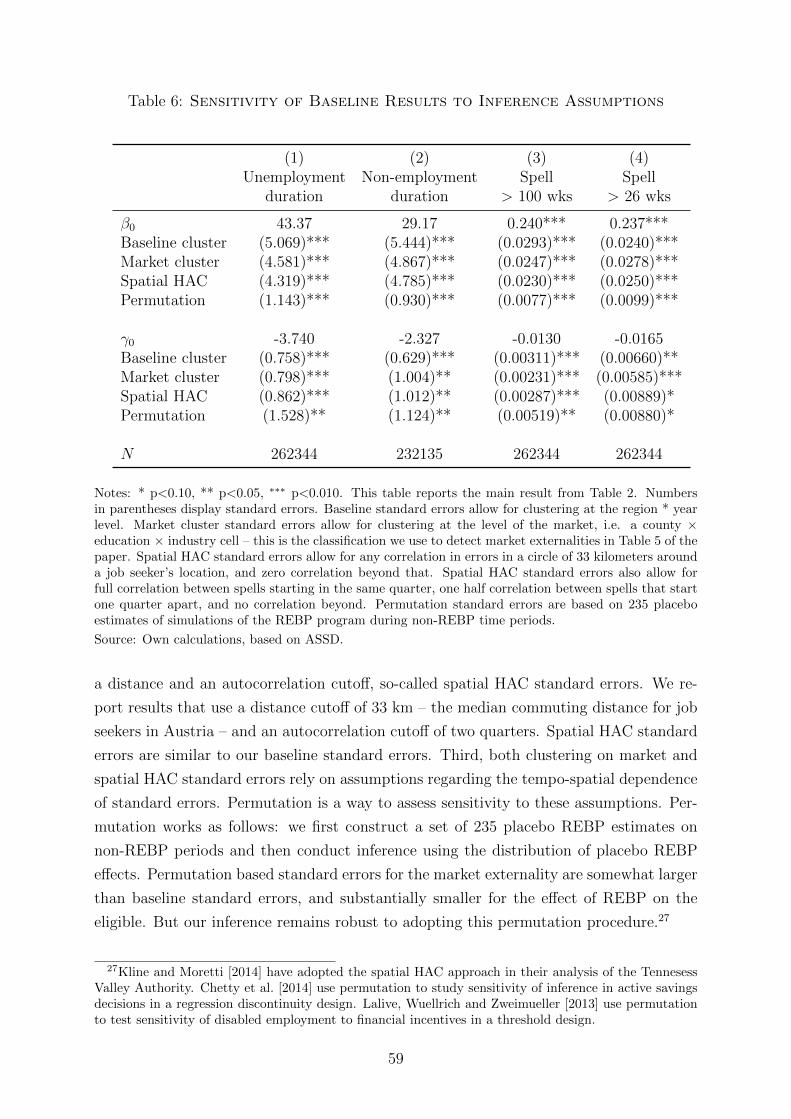
Table 6: Sensitivity of Baseline Results to Inference Assumptions

(1) (2) (3) (4)Unemployment Non-employment Spell Spell

duration duration > 100 wks > 26 wks

β0 43.37 29.17 0.240*** 0.237***Baseline cluster (5.069)*** (5.444)*** (0.0293)*** (0.0240)***Market cluster (4.581)*** (4.867)*** (0.0247)*** (0.0278)***Spatial HAC (4.319)*** (4.785)*** (0.0230)*** (0.0250)***Permutation (1.143)*** (0.930)*** (0.0077)*** (0.0099)***

γ0 -3.740 -2.327 -0.0130 -0.0165Baseline cluster (0.758)*** (0.629)*** (0.00311)*** (0.00660)**Market cluster (0.798)*** (1.004)** (0.00231)*** (0.00585)***Spatial HAC (0.862)*** (1.012)** (0.00287)*** (0.00889)*Permutation (1.528)** (1.124)** (0.00519)** (0.00880)*

N 262344 232135 262344 262344

Notes: * p<0.10, ** p<0.05, ∗∗∗ p<0.010. This table reports the main result from Table 2. Numbersin parentheses display standard errors. Baseline standard errors allow for clustering at the region * yearlevel. Market cluster standard errors allow for clustering at the level of the market, i.e. a county ×education × industry cell – this is the classification we use to detect market externalities in Table 5 of thepaper. Spatial HAC standard errors allow for any correlation in errors in a circle of 33 kilometers arounda job seeker’s location, and zero correlation beyond that. Spatial HAC standard errors also allow forfull correlation between spells starting in the same quarter, one half correlation between spells that startone quarter apart, and no correlation beyond. Permutation standard errors are based on 235 placeboestimates of simulations of the REBP program during non-REBP time periods.

Source: Own calculations, based on ASSD.

a distance and an autocorrelation cutoff, so-called spatial HAC standard errors. We re-

port results that use a distance cutoff of 33 km – the median commuting distance for job

seekers in Austria – and an autocorrelation cutoff of two quarters. Spatial HAC standard

errors are similar to our baseline standard errors. Third, both clustering on market and

spatial HAC standard errors rely on assumptions regarding the tempo-spatial dependence

of standard errors. Permutation is a way to assess sensitivity to these assumptions. Per-

mutation works as follows: we first construct a set of 235 placebo REBP estimates on

non-REBP periods and then conduct inference using the distribution of placebo REBP

effects. Permutation based standard errors for the market externality are somewhat larger

than baseline standard errors, and substantially smaller for the effect of REBP on the

eligible. But our inference remains robust to adopting this permutation procedure.27

27Kline and Moretti [2014] have adopted the spatial HAC approach in their analysis of the TennesessValley Authority. Chetty et al. [2014] use permutation to study sensitivity of inference in active savingsdecisions in a regression discontinuity design. Lalive, Wuellrich and Zweimueller [2013] use permutationto test sensitivity of disabled employment to financial incentives in a threshold design.

59

Table 7: Sensitivity analysis to sample restrictions

(1) (2) (3) (4) (5) (6)Unemployment duration Non-empl. Spell Spell

duration >100 wks >26 wks

A. Men, 46 to 59, excluding steel sector

β0 50.20∗∗∗ 44.84∗∗∗ 43.82∗∗∗ 33.60∗∗∗ 0.254∗∗∗ 0.222∗∗∗

(3.607) (3.300) (3.210) (5.165) (0.0192) (0.0155)

γ0 -2.680∗∗∗ -2.133∗∗∗ -3.222∗∗∗ -2.514∗∗∗ -0.00912∗∗∗ -0.0139∗∗

(0.782) (0.657) (0.608) (0.527) (0.00240) (0.00545)

N 378556 369477 369477 304664 369477 369477

B. Men and women, 46 to 54, excluding steel sector

β0 55.93∗∗∗ 52.28∗∗∗ 51.80∗∗∗ 40.59∗∗∗ 0.297∗∗∗ 0.238∗∗∗

(3.549) (3.472) (3.319) (5.147) (0.0192) (0.0163)

γ0 -2.241∗∗∗ -1.307∗∗ -3.217∗∗∗ -1.892∗∗∗ -0.0103∗∗∗ -0.0106∗∗

(0.781) (0.648) (0.682) (0.608) (0.00297) (0.00522)

N 359901 351433 351433 296768 351433 351433

C. Men, 46 to 54, including steel sector

β0 47.33∗∗∗ 43.82∗∗∗ 43.85∗∗∗ 30.58∗∗∗ 0.242∗∗∗ 0.238∗∗∗

(5.534) (5.108) (5.045) (5.603) (0.0290) (0.0237)

γ0 -2.248∗∗∗ -1.809∗∗ -3.581∗∗∗ -2.228∗∗∗ -0.0119∗∗∗ -0.0158∗∗

(0.825) (0.730) (0.785) (0.632) (0.00304) (0.00700)

N 284099 278021 278021 245621 278021 278021

Educ., industry,citizenship, × × × × ×marital status

Region-specific × × × ×trends

Notes: S.e. clustered at the year×region level in parentheses. * p<0.10, ** p<0.05, ∗∗∗ p<0.010.All duration outcomes are expressed in weeks. The table presents estimates of the model presented in equation (3) wherewe explore the sensitivity of our baseline results to various sample restrictions. β0 identifies the effect of REBP on eligibleunemployed, while γ0 identifies spillovers of REBP on non-eligible unemployed in REBP counties. In column (1), we estimatethis model without any other controls. In column (2) we add a vector of controls X which includes education, 15 industrycodes, family status, citizenship and tenure in previous job. In column (3) to (6) we add controls for preexisting trends byregion. Column (5) uses as an outcome the duration of total non-employment (conditional on finding employment at theend of the unemployment spell). Columns (6) and (7) use as an outcome the probability of experiencing unemploymentspells longer than 100 weeks and 26 weeks respectively. In panel A, the estimation sample includes all men age 46 to 59. Inpanel B, the sample includes all men and women age 46 to 54. In panel C, the sample is the same as our baseline samplebut also includes workers who ever worked in the steel sector.

Table 8: Robustness to REBP-counties-specific shocks: Externalities on non-eligible aged 50 to 54 using unemployed aged 30 to 39 in REBP counties as a control

(1) (2) (3) (4) (5) (6)Unemployment Non-empl. Spell

duration duration >26 wks

β0 54.32*** 50.81*** 30.30*** 30.29*** 0.312*** 0.275***(7.480) (6.784) (7.639) (7.192) (0.0432) (0.0362)

γ0 (externality) -7.878** -6.466* -7.643*** -6.347** -0.0742*** -0.0554**(3.880) (3.437) (2.156) (2.461) (0.0222) (0.0213)

Educ., marital status,industry, citizenship × × ×

N 182689 180098 170388 168163 182689 180098

Notes: S.e. clustered at the year×county level in parentheses. * p<0.10, ** p<0.05, *** p<0.010.All duration outcomes are expressed in weeks. We use the same strategy as in table 2 but we use menaged 30 to 39 in REBP counties as a control instead of men 50 to 54 in non-REBP counties. We runon a sample restricted to unemployed aged 30 to 39 and 50 to 54 a diff-in-diff specification equivalent toequation (3) where we replace M by A = 1[Age > 50]. This specification enables us to fully control forshocks to the labor markets of REBP counties contemporaneous to REBP.

61

Table 9: Externalities on non-eligible unemployed by initial level of labormarket tightness

(1) (2) (3) (4)Unemployment Non-empl. Spell Spell

REBP effect on non-treated duration duration >100 wks >26 wks

All non-eligible

γHigh θ0 ( θ ≥ P50) 0.728 -1.650 0.00877 -0.0208

(1.411) (1.088) (0.00571) (0.0125)

γLow θ0 (θ < P50 ) -2.250*** -1.809** -0.00457* -0.00936

(0.726) (0.733) (0.00255) (0.00657)

F-Test γLow θ0 = γHigh θ

0 [0.0635] [0.910] [0.0530] [0.422]

N 262109 231940 262109 262109

Non-eligible 50+

γHigh θ0 ( θ ≥ P50) -1.317 -2.788 0.00878 -0.0309

(4.073) (2.745) (0.0181) (0.0204)

γLow θ0 (θ < P50 ) -7.539*** -5.999** -0.0167** -0.0312*

(2.334) (2.407) (0.00801) (0.0180)

F-Test γLow θ0 = γHigh θ

0 [0.0530] [0.320] [0.114] [0.992]

N 122174 102598 122174 122174

Educ., marital status,industry, citizenship × × × ×

Notes: S.e. clustered at the year×region level in parentheses. * p<0.10, ** p<0.05, *** p<0.010.Sample restricted to male workers working in non-steel related sectors. All duration outcomes are expressedin weeks. The table presents estimates of the effects of REBP on non-eligible workers broken down by theinitial level of labor market tightness in county×industry×education cells. Initial labor market tightness isobtained by dividing the average monthly number of vacancies posted in 1990 (the first year for which wehave some vacancy information by county) in each county×industry×education cell, by the average monthly

number of unemployed in the same county×industry×education cell. γHigh θ0 identifies externalities of REBP

on non-treated workers in REBP county×industry×education cells where labor market tightness was abovethe median level of tightness in 1990. γLow θ

0 identifies externalities of REBP on non-treated workers in REBPcounty×industry×education cells where labor market tightness was below the median level of tightness in1990.

D Wages

D.1 Effect of REBP on reemployment wages

As highlighted in section I and explained formally in appendix section A, one of the key

requirement for externalities to be positive on non-eligible workers is that wages do not

react much to outside options of workers. Here, we investigate explicitly this question by

looking at the effect of REBP on reemployment wages and other characteristics of jobs

at reemployment.28

The identification of the effect of REBP on wages is very different from our previous

market externality analysis, as we now wish to compare eligible workers to non-eligible

workers (rather than non-eligible in treated and non treated markets). The identification

of the effect of REBP on wages is difficult for at least three reasons. First, REBP treat-

ment is correlated with longer unemployment duration, which may directly affect wages

through duration dependence effects. If reemployment wages depend on the duration of

the unemployment spell w = w(D,B) (because of human capital depreciation, or discrim-

ination from the employers), then the effect of a change in benefits B on reemployment

wage can be decomposed into two effects:

dw

dB=

∂w

∂D· ∂D∂B︸ ︷︷ ︸

Duration effect

+

Reservation wage effect︷︸︸︷∂w

∂B

If reemployment wages decline over the duration of a spell ( ∂w∂D

< 0), the total effect of an

increase in benefits on reemployment wages might be zero or even negative even though

the reservation wage effect is positive.

The second issue is that REBP treatment affects the probability of entering into unem-

ployment and REBP recipients may therefore be selected along unobserved characteristics

that are correlated with wages. Treatment is also correlated with the probability of ever

reentering the labor force, which creates additional selection issues when looking at reem-

ployment wages.

The third issue is that REBP affects labor market tightness, which will in turn affect

the bargaining power of workers. It is thus difficult to separate what is the pure reservation

wage effect from other equilibrium effects affecting wages.

We try to address these issues in the following analysis, but we want to stress that

our analysis remains tentative. To deal with the first issue, we follow the methodology

of Schmieder, von Wachter and Bender [2012a] and estimate the effect of variations in

benefits on reemployment wages conditional on unemployment duration. We do this first

28Note that Lalive [2007] discusses the effects of benefit extension programs on re-employment wageswithout conditioning on elapsed unemployment duration.

63

in the diff-in-diff setting of equation 3, and then in a RD setting taking advantage of

the age eligibility discontinuity at 50 and experience eligibility discontinuity at 15 years.

Note that in both cases, the identifying assumption requires that there is no correlation

between unobserved heterogeneity and unemployment benefits conditional on unemploy-

ment duration which is a much stronger assumption than in the standard diff-in-diff or RD

assumptions where we only need that the correlation between unobserved heterogeneity

and unemployment benefits is zero.

We plot in appendix figure 6 post-unemployment wages conditional on the duration of

the unemployment spell in REBP and non-REBP counties for eligible workers (aged 50 to

54 with more than 15 years of experience). The difference between REBP and non-REBP

counties at each duration point in panel B (when REBP was in place) compared to the

same difference in panel A (when REBP was not in place) gives us a diff-in-diff estimate of

the effect of REBP on reemployment wages conditional on spell duration. This evidence

suggests that there was no effect of REBP on reemployment wages.

We formally assess this result in appendix table 10 by running a simple diff-in-diff

model where we compare workers eligible to REBP (treatment) to non-eligible workers

(control). Each panel uses a different control group. In panel A, we use workers aged

50 to 54 with more than 15 years of experience but residing in non-REBP regions. In

panel B we use workers aged 50 to 54 residing in REBP regions but with less than 15

years of experience. In panel C we use workers aged 46 to 49 with more than 15 years of

experience and residing in REBP regions. In column (1), we estimate the model without

further controls. In column (2) we add a vector of controls including education, 15 industry

codes, family status, citizenship and tenure in previous job. These specifications tend to

deliver a negative effect of REBP on reemployment wages. This negative effect may well

be driven by selection into unemployment. We know from table 3 that REBP has affected

the inflow rate into unemployment of eligible workers. This means that the selection of

eligible workers may be different during REBP. We try to control for this using pre-

employment wages. In column (3) we add a rich set of pre-unemployment wage dummies

to control for potential differential self-selection into unemployment due to REBP. As

explained above, the negative effect on reemployment wages found in column (1) and (2)

can also be due to duration dependence effects. In column (4) we allow for an effect of

longer unemployment spells during on reemployment wages (because of skill depreciation,

employer discrimination, etc.). Following the methodology of Schmieder, von Wachter

and Bender [2012a], we condition on the duration of unemployment using a rich set of

dummies for the duration of unemployment prior to finding a new job. In this preferred

specification of column (4), irrespective of the control group we are using, we always find

no significant effect of REBP on reemployment wages.

To complement our diff-in-diff approach, we also focus on the age eligibility disconti-

nuity at 50 in REBP counties and estimate RD effects of the REBP extensions controlling

64

for the effect of duration on reemployment wages by adding a rich set of dummies for the

duration of the spell prior to finding the job.

E[Y |A = a] =

p∑p=0

[γp(a− k)p + νp(a− k)p · 1[A ≥ k]] +T∑t=0

1[D = t] (30)

where Y is real reemployment wage, A is age at the beginning of the unemployment spell,

k = 50 is the age eligibility threshold, and D is the duration of the unemployment spell

prior to finding the new job. We use a third-order polynomial specification. Results

are displayed in appendix figure 7, where we have estimated this model for six periods

to look at the dynamics of the wage response. Before REBP, we can detect no sign of

discontinuity at age 50 in reemployment wages. But interestingly, we can detect a small

discontinuity at the beginning of REBP (1988-1990). This discontinuity increases over

time and is the largest in 1991-1993, at the peak of REBP. The implied RD estimate of

the elasticity of wages with respect to UI benefits is .14 (.04). This discontinuity then

decreases and disappears when REBP is over. This suggests that wages are relatively

rigid in the short run, but that in the longer run, wages might adjust to variations in

outside options of workers. Note, however, that the McCrary test rejects continuity of

the probability density function of the assignment variable (age) at the cutoff (50 years)

during REBP. This implies that the wage effects could also partly be driven by selection

(sorting) at the 50 years age cut-off.

We finally exploit the experience eligibility discontinuity in REBP counties using the

same methodology. Results are displayed in appendix figure 9. The figure displays for

REBP regions the relationship between experience in the past 25 years at the beginning

of unemployment spell and reemployment wages for workers aged 50 to 54. We use the

discontinuity created by the fact that workers with more than 15 years of experience are

eligible for REBP extensions while workers with less than 15 years are not eligible. The

graph shows the average reemployment wage for each bin of 6 months of past experience

for all non REBP years and for all REBP years. We also estimate a model of the form:

E[Y |E = e] =∑p

p=0 γp(a− k)p + νp(a− k)p · 1[E ≥ k] +∑T

t=0 1[D = t], where Y is real

reemployment wage, E is experience at the beginning of the unemployment spell, k = 15

is the experience eligibility threshold, and D is the duration of the unemployment spell

prior to finding the new job. The graph plots the predicted values of this regression for all

non REBP years and for all REBP years using a 3rd order polynomial for the regressions.

Here, we find no evidence of an effect of REBP on reemployment wages. Note again

however that McCrary tests rejects continuity in the probability density function of the

assignment variable (experience) at the cutoff (15 years) during REBP.

Overall, this evidence, although tentative, suggests that wages of eligible workers did

not strongly respond to REBP, which is in line with the market externalities that we find.

65

Yet, we cannot exclude that these results are confounded by selection, nor can we exclude

that wages would have adjusted in the very long run.

D.2 Implications of these results for the wage setting process

What can we learn on the wage setting process from this empirical evidence? Is this

evidence, combined with other available evidence, compatible with Nash bargaining?

Note that union membership is not extremely high in Austria, and the wage setting

process is less centralized and rigid than in most continental European countries. Austria

has (formally) a decentralized system of wage negotiations. 400 collective agreements

determine a minimum wage in the particular sector/occupation where the contract applies

and the wage growth for effective wages, leaving some room for individual bargaining.

In a standard DMP model with Nash bargaining, the wage w is a weighted average of

the productivity of the worker Π (which determines the reservation price of the employer)

and of the value of remaining unemployed z (which determines the reservation price of

the unemployed):

w = βΠ + (1− β)z

The weight β corresponds to the bargaining power of the unemployed. Therefore dwdΠ

= β

and dwdz

= 1−β. In other words, the bargaining power of the workers could be identified by

the variation of wages to a change in Π or z. The main problem is that we never observe p

nor z = z(B,X), which depends not only on unemployment benefits B but also on many

other different things such as the disutility of work, etc. The Nash bargaining model is

therefore fundamentally non-identifiable. Are there nevertheless credible values of Π, z

and β that would rationalize the empirical evidence presented here? First, all the evidence

in the macro literature (see, for instance, Shimer [2005] and Hagedorn and Manovskii

[2008]) suggests that wages do not react much to productivity shocks, so that dwdΠ

is likely

to be small. This, implies that β is small. But if β is small, then wages should react a lot

to variations in the outside options of workers, i.e. the value of remaining unemployed:dwdz

and εz = dwdz· zw

should be large. Of course, we never directly observe εz. We only

observe the variation of wages to a change in unemployment benefits dwdB· Bw

= εz · ∂z∂B ·Bz

.

Given that we found dwdB· Bw≈ 0, it is difficult to believe that εz is very large, unless

∂z∂B· Bz<< 1. In other words, it is difficult to reconcile the small elasticity of w w.r.t z

and the small elasticity of w w.r.t p in the Nash bargaining model. The only solution is

to assume that Bz<< 1 as in Hagedorn and Manovskii [2008]. But two pieces of evidence

argue against such an assumption. First, if we follow their preferred calibration for β,

our largest estimate of εz would imply29 that B ≤ .05 · z which seems absurdly low. In

other words the value of remaining unemployed would be more than 20 times larger than

the value of the unemployment benefits received by an unemployed. Second, if Bz<< 1,

29Assuming an additive specification z = B + f(X) so that ∂z∂B = 1.

66

this in turn implies that accounting profits of firms Π − w are small, so that even small

increases in w have very large effects on vacancy openings by firms, driving labor market

tightness down. This means that the “wage externality” would be very large, shocking

labor demand down as in figure 5 panel B. This would also mean that the externalities

of large unemployment extension programs like REBP would likely go in the opposite

direction compared to our estimates. Overall, it seems reasonable to think that the Nash

bargaining model is maybe not the best way to describe the data. A model of wage setting

with some wage stickiness, at least in the short to medium run seems more appropriate.

Still, it does not mean that Nash bargaining is not appropriate to describe the longer

run. Indeed, the effects of REBP on wages seems to build up slightly over time and with

treatment intensity. In the very long run, wages may adjust more to B than what we

observe in the REBP experiment, suggesting that dwdz

can be larger in the long run. This

has important implications for the design of UI policies.

67

Figure 6: Reemployment wages conditional on duration of unemploymentspell in REBP and non-REBP counties

A. Before and after REBP7.

758.

258.

759.

259.

75Lo

g re

empl

oym

ent w

age

0 2 4 6 8 10 12 14 16 18 20Unemployment spell in month

REBP regions Non-REBP regions

B. During REBP

7.75

8.25

8.75

9.25

9.75

Log

reem

ploy

men

t wag

e

0 2 4 6 8 10 12 14 16 18 20Unemployment spell in month

REBP regions Non-REBP regions

Notes: the figure plots post-unemployment wages conditional on the duration of the unemployment spell in REBP andnon-REBP counties for workers aged 50 to 54 with more than 15 years of experience in the past 25 years prior to becomingunemployed. Following the methodology of Schmieder, von Wachter and Bender [2012a], by conditioning on the durationof unemployment, we control for the fact that REBP eligible workers experienced longer unemployment spells during theREBP period, which may impact reemployment wages if the distribution of wages depend on time spent unemployed(because of skill depreciation or discrimination from employers for instance). The difference between REBP and non-REBPcounties at each duration point in panel B (when REBP was in place) compared to the same difference in panel A (whenREBP was not in place) gives us a diff-in-diff estimate of the “reservation wage” effect. This evidence suggests that therewas no significant reservation wage effect of REBP.

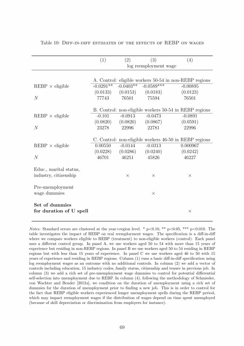
Table 10: Diff-in-diff estimates of the effects of REBP on wages

(1) (2) (3) (4)log reemployment wage

A. Control: eligible workers 50-54 in non-REBP regionsREBP × eligible -0.0291** -0.0403** -0.0589*** -0.00895

(0.0133) (0.0153) (0.0183) (0.0123)N 77743 76501 75594 76501

B. Control: non-eligible workers 50-54 in REBP regionsREBP × eligible -0.101 -0.0913 -0.0473 -0.0891

(0.0820) (0.0820) (0.0867) (0.0591)N 23278 22996 22781 22996

C. Control: non-eligible workers 46-50 in REBP regionsREBP × eligible 0.00550 -0.0144 -0.0313 0.000967

(0.0228) (0.0286) (0.0240) (0.0242)N 46701 46251 45826 46227

Educ., marital status,industry, citizenship × × ×

Pre-unemploymentwage dummies ×

Set of dummiesfor duration of U spell ×

Notes: Standard errors are clustered at the year×region level. * p<0.10, ** p<0.05, *** p<0.010. Thetable investigates the impact of REBP on real reemployment wages. The specification is a diff-in-diffwhere we compare workers eligible to REBP (treatment) to non-eligible workers (control). Each paneluses a different control group. In panel A, we use workers aged 50 to 54 with more than 15 years ofexperience but residing in non-REBP regions. In panel B we use workers aged 50 to 54 residing in REBPregions but with less than 15 years of experience. In panel C we use workers aged 46 to 50 with 15years of experience and residing in REBP regions. Column (1) runs a basic diff-in-diff specification usinglog reemployment wages as an outcome with no additional controls. In column (2) we add a vector ofcontrols including education, 15 industry codes, family status, citizenship and tenure in previous job. Incolumn (3) we add a rich set of pre-unemployment wage dummies to control for potential differentialself-selection into unemployment due to REBP. In column (4), following the methodology of Schmieder,von Wachter and Bender [2012a], we condition on the duration of unemployment using a rich set ofdummies for the duration of unemployment prior to finding a new job. This is in order to control forthe fact that REBP eligible workers experienced longer unemployment spells during the REBP period,which may impact reemployment wages if the distribution of wages depend on time spent unemployed(because of skill depreciation or discrimination from employers for instance).

69

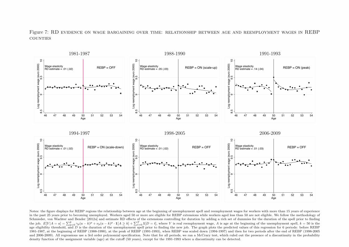
Figure 7: RD evidence on wage bargaining over time: relationship between age and reemployment wages in REBPcounties

1981-1987 1988-1990 1991-1993

Wage elasticityRD estimate = .01 (.02) REBP = OFF

8.5

99.

510

Log

reem

ploy

men

t wag

e (e

uro

2000

)

46 47 48 49 50 51 52 53 54Age

Wage elasticityRD estimate = .05 (.03) REBP = ON (scale-up)

8.5

99.

510

Log

reem

ploy

men

t wag

e (e

uro

2000

)

46 47 48 49 50 51 52 53 54Age

Wage elasticityRD estimate = .14 (.04) REBP = ON (peak)

8.5

99.

510

Log

reem

ploy

men

t wag

e (e

uro

2000

)

46 47 48 49 50 51 52 53 54Age

1994-1997 1998-2005 2006-2009

Wage elasticityRD estimate = .01 (.02) REBP = ON (scale-down)

8.5

99.

510

Log

reem

ploy

men

t wag

e (e

uro

2000

)

46 47 48 49 50 51 52 53 54Age

Wage elasticityRD estimate = .01 (.02) REBP = OFF

8.5

99.

510

Log

reem

ploy

men

t wag

e (e

uro

2000

)

46 47 48 49 50 51 52 53 54Age

Wage elasticityRD estimate = .01 (.03) REBP = OFF

8.5

99.

510

Log

reem

ploy

men

t wag

e (e

uro

2000

)

46 47 48 49 50 51 52 53 54Age

Notes: the figure displays for REBP regions the relationship between age at the beginning of unemployment spell and reemployment wages for workers with more than 15 years of experiencein the past 25 years prior to becoming unemployed. Workers aged 50 or more are eligible for REBP extensions while workers aged less than 50 are not eligible. We follow the methodology ofSchmieder, von Wachter and Bender [2012a] and estimate RD effects of the extensions controlling for duration by adding a rich set of dummies for the duration of the spell prior to finding

the job. E[Y |A = a] =∑pp=0 γp(a − k)p + νp(a − k)p · 1[A ≥ k] +

∑Tt=0 1[D = t], where Y is real reemployment wage, A is age at the beginning of the unemployment spell, k = 50 is the

age eligibility threshold, and D is the duration of the unemployment spell prior to finding the new job. The graph plots the predicted values of this regression for 6 periods: before REBP1981-1987, at the beginning of REBP (1988-1990), at the peak of REBP (1991-1993), when REBP was scaled down (1994-1997) and then for two periods after the end of REBP (1998-2005and 2006-2009). All regressions use a 3rd order polynomial specification. Note that for all periods, we ran a McCrary test, which ruled out the presence of a discontinuity in the probabilitydensity function of the assignment variable (age) at the cutoff (50 years), except for the 1991-1993 where a discontinuity can be detected.

Figure 8: Probability density function of age at the start of an unemploy-ment spell in REBP and non-REBP counties

A. Before REBP

McCrary Test:Discontinuity est.= .006 (.018)

.02

.04

.06

.08

.1.1

2Pr

obab

ility

Den

sity

Fun

ctio

n

42 43 44 45 46 47 48 49 50 51 52 53 54Age

REBP regionsNon-REBP regions

B. During REBP

McCrary Test:Discontinuity est.= .098 (.02)

.02

.04

.06

.08

.1.1

2Pr

obab

ility

Den

sity

Fun

ctio

n

42 43 44 45 46 47 48 49 50 51 52 53 54Age

REBP regionsNon-REBP regions

71

Figure 9: RD evidence on wages using experience cutoff: relationship be-tween experience and reemployment wages in REBP counties

Non-REBP period

Wage elasticityRD estimate = -.01 (.04) REBP = OFF

89

1011

Log

reem

ploy

men

t wag

e (e

uro

2000

)

7.5 10 12.5 15 17.5 20 22.5Experience

REBP period

Wage elasticityRD estimate = -.07 (.05) REBP = ON

89

1011

Log

reem

ploy

men

t wag

e (e

uro

2000

)

7.5 10 12.5 15 17.5 20 22.5Experience

Notes: the figure displays for REBP regions the relationship between experience in the past 25 years atthe beginning of unemployment spell and reemployment wages for workers aged 50 to 54. Workers withmore than 15 years of experience are eligible for REBP extensions while workers with less than 15 yearsare not eligible. We follow the methodology of Schmieder, von Wachter and Bender [2012a] and estimateRD effects of the extensions controlling for duration by adding a rich set of dummies for the duration ofthe spell prior to finding the job. E[Y |E = e] =

∑pp=0 γp(a−k)p+νp(a−k)p ·1[E ≥ k] +

∑Tt=0 1[D = t],

where Y is real reemployment wage, E is experience at the beginning of the unemployment spell, k = 15is the experience eligibility threshold, and D is the duration of the unemployment spell prior to findingthe new job. The graph plots the predicted values of this regression for all non REBP years and for allREBP years using a 3rd order polynomial for the regressions.