Embed Size (px)
Citation preview

Advances in Management & Applied Economics, vol. 6, no.1, 2016, 47-67
ISSN: 1792-7544 (print version), 1792-7552(online)
Scienpress Ltd, 2016
Market Concentration in the Grocery Retail
Industry: Application of the Basic Prisoners’
Dilemma Model
Fidel Ezeala-Harrison1 and John Baffoe-Bonnie
2
Abstract
We assess spatial concentration ratios in the grocery retail industry across four
regions of the country to determine whether there is evidence of covert collusion
among the retail chains that can explain why we do not see more price competition
among them. We apply a basic theory of the prisoners’ dilemma game model,
together with an empirical analysis that utilizes the price-concentration model
(PCM) to test both the direction and size of the effect of concentration on prices,
whilst controlling for other factors that affect the retail prices of the grocery retail
firms. The work explores whether higher concentration does enable collusive
behavior that leads to higher set prices of grocery products within and across
given spatial locations, by estimating a PCM which allows us to verify the extent
to which the grocery retail chains can manipulate and set prices uniformly among
themselves in a quasi-collusive behavior.While the theory suggests that the degree
of competition as opposed to cooperative collusive outcomes in the industry
depends on the accuracy of rival conjectures about each other's moves, the
empirical evidence indicates that the pricing patterns observed between the
companies may be largely due to covert tacit collusion among these retail firms.
JEL classification numbers: L11, L13, C5, C7
Keywords: market concentration, prisoners’ dilemma, grocery price concentration
1Professor of Economics, Jackson State University, USA
2Professor of Economics, Penn State University, Media, PA, USA
Article Info: Received : September 12, 2015. Revised : October 12, 2015 Published online : January 30, 2016.
48 Fidel Ezeala-Harrison and John Baffoe-Bonnie
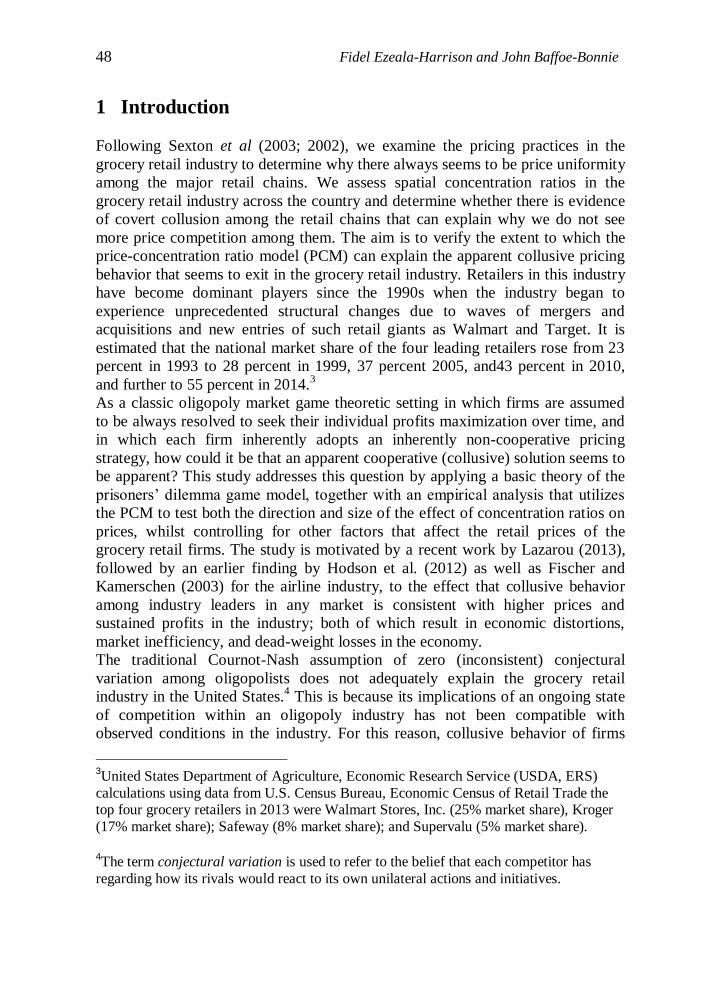
1 Introduction
Following Sexton et al (2003; 2002), we examine the pricing practices in the
grocery retail industry to determine why there always seems to be price uniformity
among the major retail chains. We assess spatial concentration ratios in the
grocery retail industry across the country and determine whether there is evidence
of covert collusion among the retail chains that can explain why we do not see
more price competition among them. The aim is to verify the extent to which the
price-concentration ratio model (PCM) can explain the apparent collusive pricing
behavior that seems to exit in the grocery retail industry. Retailers in this industry
have become dominant players since the 1990s when the industry began to
experience unprecedented structural changes due to waves of mergers and
acquisitions and new entries of such retail giants as Walmart and Target. It is
estimated that the national market share of the four leading retailers rose from 23
percent in 1993 to 28 percent in 1999, 37 percent 2005, and43 percent in 2010,
and further to 55 percent in 2014.3
As a classic oligopoly market game theoretic setting in which firms are assumed
to be always resolved to seek their individual profits maximization over time, and
in which each firm inherently adopts an inherently non-cooperative pricing
strategy, how could it be that an apparent cooperative (collusive) solution seems to
be apparent? This study addresses this question by applying a basic theory of the
prisoners’ dilemma game model, together with an empirical analysis that utilizes
the PCM to test both the direction and size of the effect of concentration ratios on
prices, whilst controlling for other factors that affect the retail prices of the
grocery retail firms. The study is motivated by a recent work by Lazarou (2013),
followed by an earlier finding by Hodson et al. (2012) as well as Fischer and
Kamerschen (2003) for the airline industry, to the effect that collusive behavior
among industry leaders in any market is consistent with higher prices and
sustained profits in the industry; both of which result in economic distortions,
market inefficiency, and dead-weight losses in the economy.
The traditional Cournot-Nash assumption of zero (inconsistent) conjectural
variation among oligopolists does not adequately explain the grocery retail
industry in the United States.4 This is because its implications of an ongoing state
of competition within an oligopoly industry has not been compatible with
observed conditions in the industry. For this reason, collusive behavior of firms
3United States Department of Agriculture, Economic Research Service (USDA, ERS)
calculations using data from U.S. Census Bureau, Economic Census of Retail Trade the top four grocery retailers in 2013 were Walmart Stores, Inc. (25% market share), Kroger
(17% market share); Safeway (8% market share); and Supervalu (5% market share).
4The term conjectural variation is used to refer to the belief that each competitor has
regarding how its rivals would react to its own unilateral actions and initiatives.

Market Concentration in the Grocery Retail Industry... 49
designed to limit competition and enable colluding members to set high prices and
thereby earn profits above the normal competitive level seems to exist in the
grocery retail industry. Although such practices are prohibited under both Federal
and State statutes in order to protect consumers, and considerable resources are
allocated each time to prosecute such antitrust violations, yet the very outcomes
that are targeted for prevention appear to often emerge.
Leading research studies on market power and collusive pricing behavior such as
Fischer and Kamerschen (2003),Baraji and Ye (2003), Baraji and Summers
(2002), or Pesendorfer (2000), have established proof for the existence of
monopoly power, and concluded that retail prices across most industries are also
influenced by the particular region of the country under consideration at any time.
Benson and Faminow (1985) had established the widely held fact that grocery
retailing had always been essentially oligopolistic in terms of pricing behavior.
More recent studies have stressed this finding; for example, Bajari and Ye (2003)
carried out an analysis that computed the probabilities that observed outcomes in
the industry are the result of competitive behaviors of firms that fail the tests for
conditional market independence. In a study of the perishable fresh produce retail
chains, using nation-wide data, Sexton et al. (2003) found that the structure of
grocery retailing necessarily gives large retailers some degree of market power in
terms of the ability to influence price; and concluded that to the extent that
retailers exercise their market power in the sense of marking up prices in excess of
full marginal costs, they exploit the unilateral monopoly power they possess
through geographic and brand differentiation. Similarly, Binkley and Connor
(1998)cited the work ofHoch et al. (1995) which developed four competitive
variables to explain store-level price-elasticities of 18 branded grocery products.
The authors examined the effects of warehouse-type stores within the given
geographical location, and found that such presence resulted in increased elasticity
of demand and therefore more competitive prices, while the distance from such
stores (including those outside the immediate trading area) negatively affected the
responsiveness of demand to price variations. The findings were supported by
Drescher and Connor (1999) which also found that the presence of warehouse-
type stores significantly reduced overall market grocery prices.
Preceding studies focussing on how truly competitive the grocery retail industry
is, and the impact of the degree of concentration on prices in the grocery retail
industry, include Connor (2001), Yu and Connor (1999), Dobson and Waterson
(1997), as well as Cotterill (1991, 1986).
Yu and Connor’s (1999) study revealed that some price competition existed in the
industry in terms of rivalry between the major industry leaders in the horizontal,
vertical, and geographic dimensions. The study applied empirical cross-sectional
analysis of retail price competition, and found that in the case of horizontal price
competition, pricing was sensitive to different degrees of firm concentration in the
industry; thus, differences in overall grocery prices across geographic markets in
the industry existed in terms of competitive intensity as measured by market
shares and/or market concentration.

50 Fidel Ezeala-Harrison and John Baffoe-Bonnie
Cotterill and Harper (1995), drawing upon an earlier study that applied highly
aggregated retail food price indexes published for 18 large U.S. metropolitan areas
by the Bureau of Labor Statistics (Lamm, 1981), which found that industry
concentration was positively related to food prices, also verified and concluded
that there existed a positive industry concentration-price relationship for a sample
of 34 local markets in and around Arkansas. Connor (2001) cited a 1999 study
(Drescher and Connor, 1999) in which, aided by a 1993 special survey of
consumer prices across 50 German cities and a comprehensive commercial data
base on grocery stores, they established a relationship between the industry 5-firm
concentration ratio (CR5) and grocery retail prices. The study found that as the
industry’s CR5 increased toward the study’s sample mean of 88 percent, prices
declined in the amount of 1.6 percentage points; but when the CR5 increased from
88 percent toward 100%, the resulting market power caused prices to increase by
about 3.4 percentage points from their lowest levels.
Drawing from the Drescher-Connor approach of exploring causality between
industry prices and concentration ratios, the present paper attempts to explain the
basis of collusive pricing patterns in the grocery retail industry, whereby we
investigate the impact of the industry’s four-firm concentration ratio (CR4)and
pricing, and use it to establish evidence of collusive pricing behavior on the part of
industry leaders. We apply the framework of basic prisoners’ dilemma game
theoretic analysis to explain grocery pricing in the context of oligopoly market
rivalry in which a competitor's conjectural variation about rival moves is strictly
non-zero with a probability of being either correct or incorrect. The analysis is
used to determine whether grocery retail pricing is based on cooperative (quasi-
collusive) or non-cooperative (competitive) strategies, depending on whether or
not rival conjectures about each others' moves and responses turn out to be
certain.5
2 Resolving the Prisoners' Dilemma in a System of Finite
Repeated Games
Being a classic case of oligopoly market rivalry in which a competitor's
conjectural variation about rival moves is strictly non-zero, the Prisoners'
Dilemma model can be used to convey the central message of this paper, namely,
the use of the probability that each competitor's conjectural variation could be
either right or wrong in devising long term strategic dispositions. This is
particularly so where the conjecture is about whether or not rivals would act
cooperatively. Moreover, the grocery retail market involves a system where
5We assume that playing cooperatively would imply raising prices, while a non-
cooperative play would imply a drastic price reduction.

Market Concentration in the Grocery Retail Industry... 51
competitors can (and do) choose to either cooperate or not cooperate with rivals --
a system of a finite repeated game setting. For this reason, the prisoner's dilemma
framework lends itself for elucidating the main theme of the present study. In
particular, it enables us apply a simple Bayesian comparative analysis of expected
profits to explore what motivates competitors to either cooperate or not cooperate
with their rivals.
We postulate that oligopolists would not choose the cooperative solution if they
could not be more trusting of their rivals, and moreover such a trusting
relationship must be necessary for any lasting cooperative outcome. Firms are
rational and know that their rivals are also rational; and each competitor's
conjecture about its rivals' moves is correct, but might be wrong; this is because
each competitor needs not be perfectly rational (under circumstances of which its
rival's conjectural variation would be wrong).
We depict the profit payoff of each competitor by π, and assuming just two
competitors, Firm 1 and Firm 2, each of who adopt either of the two strategies of
cooperative moves (coop) with possible payoff π1 if rival adopts a similar strategy,
or payoff π-1
(losses) if rival plays non-cooperatively (noncoop). Each firm
receives payoff π0 -- indicating a bare breakeven condition -- under a mutually
aggressive (noncoop) setting, a competitive “warfare” setting. A firm reaps payoff
π2 should its rival play cooperatively while it plays aggressively. This payoff
matrix is stated as follows:
Firm 2
coop noncoop
--------------------------------------------
coop π11, π2
1 π1
-1, π2
2
Firm 1 (1)
noncoop π12, π2
-1 π1
0, π2
0
--------------------------------------------
Presumably, since the competitors are involved in their respective dominant (best)
strategies, each having a profit level π0, if and whenever a competitor's conjecture
is wrong, that competitor realizes profits π2>π
0 since its rival had failed to adopt
the best strategy.
The expected value of payoffs over the relevant time horizon for a firm adopting
aggressive (non-coop) strategy, Eπinc
, is:
Eπinc
= [ρiπi0+(1-ρi)πi
2]1 + [ρiπi
0 + (1-ρi)πi
2]2 +….
...+ [ρiπi0+(1-ρi)πi
2]k-1+[ρiπi
0+(1-ρi)πi
2]k (2)
where
ρi = probability that firm i's conjecture is correct,
πi0 = normal payoff under correct conjectures,

52 Fidel Ezeala-Harrison and John Baffoe-Bonnie
πi2 = payoff if conjecture is wrong,
and πi2>πi
0,πi
-1< 0,
i = 1, 2,..n,
k = time period 1, 2, 3….k.
Expression (2) gives the sum of current and future profits weighted by the
conjectural disposition probabilities. For a player adopting an aggressive (non-
cooperative) strategy that would result in "warfare", the expected value of payoff
would be less desirable than that obtained from a cooperative stance. The
prospects of this outcome compels the competitor to adopt a cooperative stance in
the game. However, a competitor's conjecture could be wrong (i.e. its rivals may
not really match its strategic moves in a tit-for-tat fashion), in which case the
player comes off with a larger payoff πi2. But since the game is a repetitive one,
the player could be sure of the tit-for-tat reaction down the horizon should it play
aggressively at any stage. It is this possibility that compels players to play
cooperatively, resulting in a cooperative solution in an otherwise inherently non-
cooperative game setting.
The expected payoff from cooperative play, Eπic, is
Eπic = [ρiπi
1+ (1-ρi)πi
-1]1 + [ρiπi
1+ (1-ρiπi
-1]2+…
...+ [ρiπi1+(1-ρi)πi
-1]k-1+[ρiπi
1+(1-ρi)πi
-1]k, (3)
A player's disposition at any stage of the game over time can be found by
comparing Eπinc
and Eπic at that stage. This is given by:
Eπinc
-Eπic = ρiπi
0+(1-ρi)πi
2-[ρiπi
1+(1-ρiπi
-1)],
= ρiπi0+(πi
2-πi
-1)+ρi(πi
-1-πi
2)-πiΠi
1
= (πi2-πi
-1)+ρi(πi
0-πi
1)+ρi(πi
-1-πi
2)
= πi2(1-ρi)+ρiπi
0-πi
-1(1+ρi)-πi
-1> 0 (4)
since πi-1
<0
This indicates that under a given probability of the correctness of a firm's
conjectures about rival behaviors, ρi (that is, firm iis not certain about the direction
of rival responses to its own behavior), its expected payoff would be greater by
adopting an aggressive play rather than a cooperative play. Therefore, the
condition that ρi be an indicator of an ordinary chance event (ρi<1) cannot explain
the choice of cooperative solution among oligopolists. We must turn to an
alternative condition surrounding ρi. Hence, cooperative behavior among
oligopolists, a quasi-monopolistic outcome, involves a degree of certainty among
the players regarding each other's expected actions and reactions. This rules out
the uncertainty of rivals' behavior and therefore rules out the existence of the
oligopolistic competition. This is to say that the probability of accuracy of firm is
conjectures about rivals' behaviors, is one (ρi=1). In this case equation (5) would
turn out to be:

Market Concentration in the Grocery Retail Industry... 53
Eπinc
-Eπic = πi
2-πi
-1+πi
0-πi
1+πi
-1-πi
2
= πi0-πi
1< 0. (5)
This demonstrates that only if a firm has correct conjectures about rival actions
that it is profitable for it to adopt a cooperative play, under which it would have no
incentive to deviate unilaterally. In fact, cooperative solution requires that the
firm's conjectures be certain. A firm that opts out of the cooperative stance loses
the certainty (assurance) about rivals' responses (ρi<1), and would have a lower
(non-cooperative) expected profit.
In practice, the extent of collusion between independent firms is limited by laws
on restrictive practices. Clearly, this points to a policy question concerning the
operation of the country's Competition Act under the Anti-Trust Laws. But if the
profit gains from collusion are substantially high relative to the costs of operating
the collusive agreement (including fines and any other types of punitive
liabilities), then the companies have incentives to operate the collusive
agreements. We examine this question in the empirical section below by
estimating a price-concentration model for the grocery industry across four
regions in the U.S., which allows us to verify the extent to which the grocery retail
chains can manipulate and set prices uniformly among themselves in a quasi-
collusive behavior. The PCM is applied to explore whether higher concentration
does enable collusive behavior that leads to higher set prices of grocery products
within and across given spatial locations.
One central message from the preceding game theoretic analysis is that collusive
behavior within an oligopoly industry such as grocery retail, results in high
concentration; and since the payoffs in the theoretical model represent profits of
the retail firms, which are correlated with the prices, it implies that firms tend to
adopt cooperative play (collusion) because they obtain higher profit payoffs from
doing so. Thus, since prices determine profits, we apply the profit-concentration
model that uses cross-sectional data on a mix of explanatory variables such as
store-level information, market characteristics, and geographical location, to
estimate an equation system that enables us to better understand the pattern of
pricing behavior in the grocery retail industry in the empirical analysis that
follows.
3 Empirical Analysis
3.1 Model specification and estimation
For several decades various economic and business theories have been
propounded to analyze the relationships between profits, prices and market
concentration. The profit-concentration studies found a weak positive correlation
between market concentration and profits. This finding was interpreted as an
54 Fidel Ezeala-Harrison and John Baffoe-Bonnie
evidence of collusion among leading/dominant firms in highly concentrated
industry. This assertion by the profit-concentration studies has been criticized on
the grounds that efficient firms can be expected to earn both high market shares
and high profits (efficiency rents) thereby suggesting a more benign explanation
for the observed correlation (Woodrow, 1995). This superiority or efficiency
critique expressed by Demsetz (1973) and other profit-concentration problems
have given rise to price-concentration studies. There are several advantages of
using prices as op- posed to profits. First, prices are easier to obtain than economic
profits. Second, prices are not subject to accounting conventions that complicate
the study of profits. Third, price-concentration studies are not subject to the
efficiency or the competitive superiority criticism since prices are determined in
the market.6
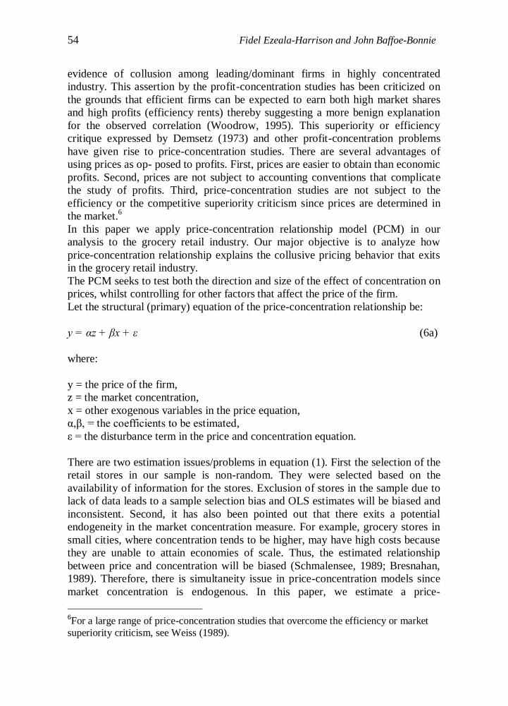
In this paper we apply price-concentration relationship model (PCM) in our
analysis to the grocery retail industry. Our major objective is to analyze how
price-concentration relationship explains the collusive pricing behavior that exits
in the grocery retail industry.
The PCM seeks to test both the direction and size of the effect of concentration on
prices, whilst controlling for other factors that affect the price of the firm.
Let the structural (primary) equation of the price-concentration relationship be:
y = αz + βx + ε (6a)
where:
y = the price of the firm,
z = the market concentration,
x = other exogenous variables in the price equation,
α,β, = the coefficients to be estimated,
ε = the disturbance term in the price and concentration equation.
There are two estimation issues/problems in equation (1). First the selection of the
retail stores in our sample is non-random. They were selected based on the
availability of information for the stores. Exclusion of stores in the sample due to
lack of data leads to a sample selection bias and OLS estimates will be biased and
inconsistent. Second, it has also been pointed out that there exits a potential
endogeneity in the market concentration measure. For example, grocery stores in
small cities, where concentration tends to be higher, may have high costs because
they are unable to attain economies of scale. Thus, the estimated relationship
between price and concentration will be biased (Schmalensee, 1989; Bresnahan,
1989). Therefore, there is simultaneity issue in price-concentration models since
market concentration is endogenous. In this paper, we estimate a price-
6For a large range of price-concentration studies that overcome the efficiency or market
superiority criticism, see Weiss (1989).

Market Concentration in the Grocery Retail Industry... 55
concentration model that addresses both the sample selection and the endogeneity
of the covariate (z).
In order to address the sample selection bias and the endogeneity of the covariate
(concentration) variable, we specify the model as:
y = αz + βx + ε (6b)
z = m + v (7)
d = w + u (8)
and
𝑑 = 1 𝑖𝑓 𝜃𝑤 + 𝑢 ≥ 00 𝑖𝑓 𝜃𝑤 + 𝑢 < 0
9
where m is the exogenous variable in equation (7), d is an indicator function, w is
the exogenous variable in equation (8), and v,u are disturbance terms in equations
(7) and (8), respectively. The first equation (6b) is the structural equation of
interest and it is the same as equation (6a). The second equation is the endogenous
concentration equation. It is the reduced form equation for the endogenous
variable z. The third equation is the selection equation; it is the probit equation
that represents the probability of being in the market or the propensity for the firm
to sell or the probability of being in the sample. The explanatory variables (w) in
equation (8) include most of the explanatory variables in equation (1a) plus other
explanatory variables that determine d. We assume that (i) (w, d) are always
observed, (ii) (y, z) are observed when d = 1, (iii) (ε, u) is independent of w with
zero mean [E(ε,u) = 0], (iv) u∼N(0,1), (v) E(w,u) = 0. Assumption (v) indicates
that we need an instrument that is correlated with z but is not correlated with or
orthogonal to the disturbance term (v). Assuming a joint multinormal distribution,
the conditional disturbance terms in equations (6b)-(8) for the entire population is
given by (ε, v, u) ∼N (0, Σ) and the variance-covariance matrix of the disturbance
term is:
= 𝐶𝑜𝑣 ℰ,𝑣,𝑢 = 𝜎𝜀
2𝜌𝜀𝑣𝜌𝜀𝑢𝜌𝑣𝜀𝜎𝑣
2𝜌𝑣𝑢𝜌𝑢𝜀 𝜌𝑢𝑣 1
From these assumptions the Heckman’s inverse Mill’s ratio (λ) can be written as:
𝜆 𝜃𝑤 = 𝜙(𝜃𝑤)
Φ(𝜃) (10)

56 Fidel Ezeala-Harrison and John Baffoe-Bonnie
where 𝜙 is the density function for standard normal distribution and Φ is the
cumulative
distribution for standard normal variable.
After adjusting for sample selection bias and using instrument for the endogenous
variable, the equation of interest is specified as:
y = 𝛼𝑧 + 𝛽𝑥 + 𝜌𝜆 + 𝜀 (11)
The ρ is the coefficient of λ and it measures the covariance between the two
residuals ε and u. Under the null hypothesis that there is no selectivity bias, we
have ρ = 0. This can be tested by means of a conventional t-test.
3.2 Data source and description
The estimation of the model discussed in section 3.1 requires store level
information, market characteristics, geographical, and other socio-economic
indicators. The model was estimated using cross-section data from different
sources. The bulk of the individual grocery retail data come from the ”Chain Store
Guide (CSG).” The CSG is a private owned U.S. company that collects
information on about 3000 grocery, supermarket and C-stores retailers across the
United States. The database has in-depth information with sales and unit history,
areas of operation, the number of employees, sales for different items, wages, cost
of operation, store location, postal area, prices of different items, and many more
variables for each grocery retail store in the database. The C-stores include Publix,
Safeway, Walmart, 7 Eleven, Costco and Whole foods. For a store to be included
in the grocery retailers and supermarket chain database, a food retailer must
operate two or more locations that generate at least 2 million dollars in grocery
sales. And for convenience stores retailer leads must operate two or more stores,
usually between 2,000-5,000 square feet with emphasis on high sales volume and
fast moving products. This indicates that the sample does not include small stores
that are unknown nationally. The regional, state and local variables such as
unemployment rate, population, and population growth were obtained from
Occupational Employment Statistics by the Bureau of Labor Statistics. The
NAICS 445100–Grocery Stores provides data for both metropolitan and non-
metropolitan areas. Other variables such as household income and household
expenditures in different areas are taken from the US Census of Retail Trade
(CRT).
Our sample consists of major grocery retail stores that operate in the United States
and that sold similar items in 2009. We selected grocery stores that operate in the
four regions. The division of states into regions is based on the Bureau of the
Census Classification-Northeast, Midwest, South and West. Each region is
Market Concentration in the Grocery Retail Industry... 57
represented by some selected cities.7 Seven parent stores are selected from each
region. We then select twenty stores from each of the seven parent stores located
in each region. This gives a total of 140 stores in each region. The selection of the
twenty stores in each region is based on the availability of information on the
variables in the model. Stores that did not have most the variables in the model
were not selected. In the Northeast and the West, many stores have a lot of
information for the variables in the model, compared to other regions, but to be
consistent with the number of firms in each region, we selected only twenty stores.
Three parent retail stores are ubiquitous in the country. These are Walmart, Target
and Sam Club. These parents stores are part of the seven parent stores in each
region. The parent grocery retail stores in each region are: (i) Northeast
(Pathmark, B.J stores, Giants, Shop Rite, Walmart, Sam Club, and Target); (ii)
Midwest (Acme, Kroger, Aldi, Save-a- lot, Walmart, Sam Club, Target); (iii)
South (Publix, Winn-Dixie, Piggly-Wiggly, Food Lion, Walmart, Sam Club, and
Target); (iv) West (Albertsons, Safeway, Costco, Whole Foods, Walmart, Sam
Club, and Target). We concentrate on two items: Food items andnon-food items of
the same brand. Food items include cereals products; Diary products; meat,
poultry, and eggs, while non-food items comprise laundry and cleaning products.
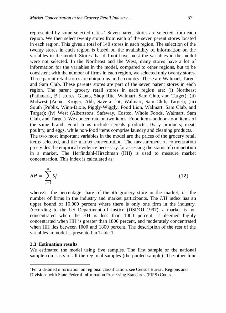
The two most important variables in the model are the prices of the grocery retail
items selected, and the market concentration. The measurement of concentration
pro- vides the empirical evidence necessary for assessing the status of competition
in a market. The Herfindahl-Hirschman (HH) is used to measure market
concentration. This index is calculated as:
𝐻𝐻 = 𝑆𝑖2
𝑛
𝑖=1
(12)
whereSi= the percentage share of the ith grocery store in the market; n= the
number of firms in the industry and market participants. The HH index has an
upper bound of 10,000 percent where there is only one firm in the industry.
According to the US Department of Justice (USDOJ 1997), a market is not
concentrated when the HH is less than 1000 percent, is deemed highly
concentrated when HH is greater than 1800 percent, and moderately concentrated
when HH lies between 1000 and 1800 percent. The description of the rest of the
variables in model is presented in Table 1.
3.3 Estimation results
We estimated the model using five samples. The first sample or the national
sample con- sists of all the regional samples (the pooled sample). The other four
7For a detailed information on regional classification, see Census Bureau Regions and
Divisions with State Federal Information Processing Standards (FIPS) Codes.

58 Fidel Ezeala-Harrison and John Baffoe-Bonnie
samples are the regional samples. Equations (6b) to (10) were estimated using the
following steps: First, we estimate a probit model using equation (8) with d as the
dependent variable and w as the explanatory variables. The estimates of the probit
model (𝜃 ) are used to calculate the inverse Mill’s ratio (λ) for each observation.
Second, using a two stage least squares approach (2SLS), we estimate the
concentration equation (7) with the exogenous variables (m) and the sample
selection variable (𝜆 ).8 Using the mean values of the explanatory variables in equation (7), we predict a
value for the concentration variable (z) and replace the concentration variable by
its corresponding predicted value.9 This imputed concentration variable (𝑧 ) serves
as an instrument for the concentration variable (z). It must be noted that the
instrumental variable technique is justified if appropriate instrument can be found.
The correlation between the actual concentration variable (HH) and the imputed
concentration variable (𝑧 ) was about 0.72. Third, we estimate the price equation
(11) by including the predicted value for the concentration variable (𝑧 ), and the
inverse Mill’s ratio (𝜆 ) as explanatory variables.10
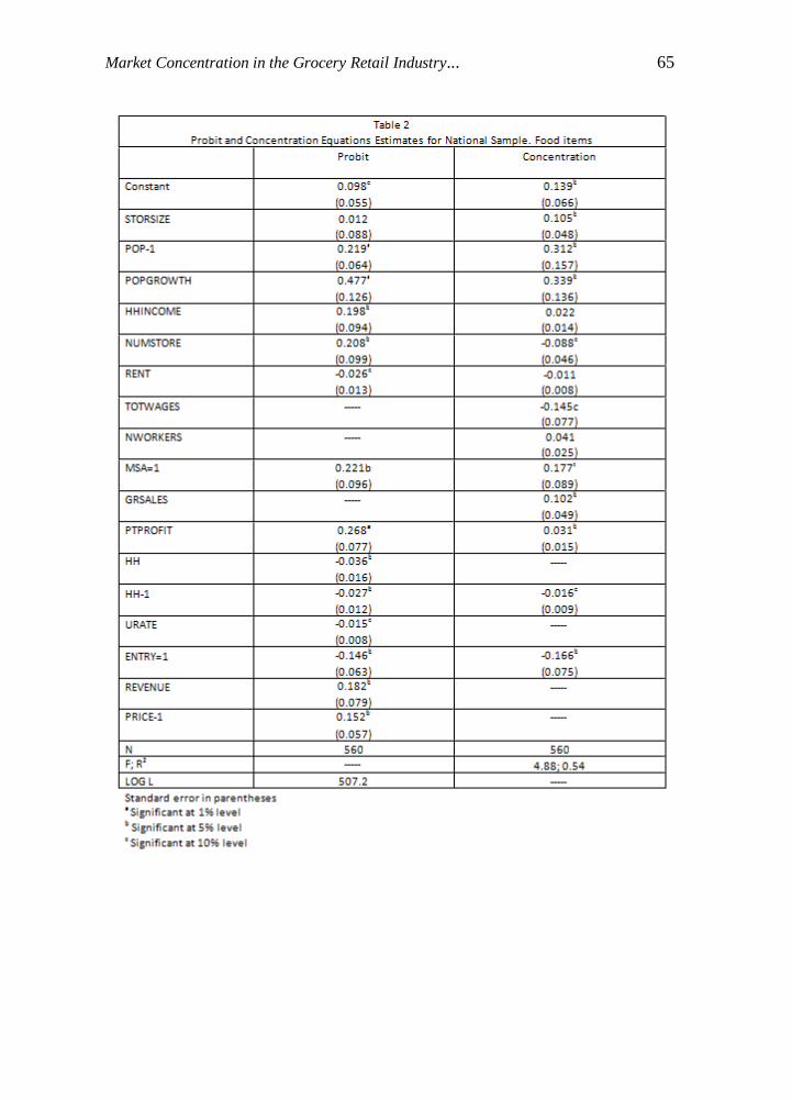
3.4 The Probit and Concentration Equations Estimates Results
Table 2 presents the probit and the concentration estimates for the national
sample.11
With the exception of the number of stores located in a particular area,
all the variables in the probit equation are statistically significant. We observe that
the population growth, the mean household income, the metropolitan area, past
profit and the market price are more likely to encourage a grocery store to engage
or be part of the grocery chain. However, past market concentration of a locality,
the entry condition, the unemployment rate may discourage a participation in the
grocery retail market. We noticed that market concentration depends positively on
8Both the order and rank conditions for identification indicates that equation (7) is over-
identified, and hence using 2SLS estimation approach is justified. 9The dependent variable of the probit equation takes a value of 1 if the firm’s profit is
greater than or equal to zero, and zero if the form’s profit is less than zero. The argument
here is that a firm will consider participating in the selling of a product in the market if
existing firms are making some profit. 10
If the instrumental variable technique is to produce consistent parameter estimate, care
must be taken in selecting instruments. First, the instruments selected must be strongly
correlated with the variable to be instrumented. In most cases, it is difficult to find such variables. Secondly, it is also almost impossible to check the assumption that the
instrumental variables are independent of the error term in the equation in which the
instrumental variables become regressors. Thirdly, one cannot be sure that the chosen variables will yield the minimum asymptotic variance. Thus the instrumental variable
technique gives priority to consistency, and pays less attention to the possibility of high
standard errors which the instrumental variables may produce. Therefore the best
instrument for a variable is the predicted value of that variable. 11
The probit and concentration results for other samples are available upon request.

Market Concentration in the Grocery Retail Industry... 59
the size of the store, population and population growth, the mean household
income, past profits of stores, and the metropolitan areas. The sample selection
bias variable is also positive and significant.
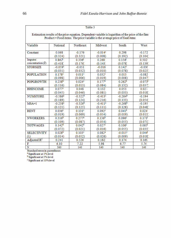
3.5 The Price Equation Estimates Results
We estimated the price equation for two groups of products -- food and non-food
items. In Table 3, the average price of the selected food is a function of some
covariates that are deemed likely to influence the prices of food. In the national
sample, the coefficient of the concentration variable is positive and significant. A
higher concentration retail food market leads to a higher average price of food.
This seems to suggest that a high concentration food market may lead to collusion.
A few grocery retail stores in a locality are more likely to collude in order to
increase the price of food in that locality. The results indicate that an increase in
population and population growth in the locality where these stores operate leads
to an increase in food prices. A plausible explanation is that an increase in the
population growth increases the demand for food and all things being equal, food
prices will rise in response to the increase in demand. Similarly, as the income of
households rise, the demand for food rises and food prices rise. We note that as
the number of stores increases in an area, the price of food decreases, probably
due to either an increase in supply of food or an increase in competition. Also
stores located in metropolitan areas have lower prices compared to non-
metropolitan areas. As expected all the cost variables have the expected signs. An
increase in rent and wages increases the cost of the stores that is likely to be
passed on to consumers in the form of higher prices. Similarly, as the store
employs more workers, the cost of the store goes up and the stores are likely to
increase food prices. The sample selection bias term is positive and significant.
This means there would have been a positive sample selection bias in the price
equation if the selection bias term was ignored.
There is a consistent result for the price-concentration relationship in all the
regions. The result indicates that as the market become more concentrated, prices
of food rise. The largest price increase is in the West as evidenced by the size of
the coefficient of the concentration variable. With the exception of the South, a
larger store size reduces food prices. Similar to the national results, an increase in
population or population growth tends to increase food prices in the Northeast,
Midwest and the South. However, the store size has an opposite effect in the West.
A larger store size reduces food prices in the West.
We observed that the magnitude of the household income, the number of stores
and the store expenditures variables (rent, wages) are quite similar to the national
results. The difference lies in the sizes of the estimated coefficients. For example,
the number of stores has the largest impact on food prices in the Midwest and least
impact in the West. Similarly, the Midwest region experiences the most price
declining effect as result of an increase in the number of stores operating in a
metropolitan area. We also found that, with the exception in the South, there was a
positive sample selection bias in the regional price equations.

60 Fidel Ezeala-Harrison and John Baffoe-Bonnie
Table 4 shows the price equation results for non-food items. The estimates of the
non- food items are quite similar to the food items results, but there are a few
differences. First, while the number of stores has mostly an inverse relationship
with the price of food, the relationship is direct in the non-food price equation.
The population variable is positive in the West region equation. Second, the size
of the coefficient of the concentration variable is larger in the non-food equations
than in the food equations for all regions. That is, market concentration has more
impact on the prices of non-food than food prices. A plausible explanation may be
that the demand for food may be price-inelastic compared to non-food items.
Third, with the exception in the Northeast, there is a negative sample selection
bias in regional price equations.
5 Conclusion
This paper has applied the prisoners’ dilemma game model together with an
empirical analysis that utilizes the price-concentration model (PCM) to determine
whether higher concentration does enable collusive behavior that leads to higher
set prices of grocery products within and across regional locations in the U.S. We
estimated a system of PCM equations to verify the extent to which the grocery
retail chains can manipulate and set prices uniformly among themselves in a
quasi-collusive behavior.The theory suggests that the degree of competition as
opposed to cooperative collusive behavior in the industry depends on the accuracy
of rival conjectures about each other's moves because oligopoly firms are less
likely to adopt any aggressive strategies that might lead to accelerated competition
that might jeopardize chances of higher profits; although, if firms believe that
rivals are less than perfectly rational (and such a belief turns out to be rightly so),
then they may resort to aggressive postures that result in non-cooperative
strategies and quasi-competitive outcomes.
The empirical analysis shows a consistent result for the price-concentration
relationship in all the regions. It indicates that as the market become more
concentrated, prices of grocery products rise, with the largest price increase
occurring in the West as evidenced by the magnitude of the coefficient of the
concentration variable; while, with the exception of the South, a larger store size
reduces grocery prices. These results may suggest that the pricing patterns
observed between the retail companies in the grocery industry may be largely due
to covert tacit collusion among these retail firms, whereby each firm seems to
adopt a strategy that results in a cooperative solution in an otherwise inherently
non-cooperative game setting. This appears to bear out evidence of a general
tendency for quasi-price fixing at best, and outright tacit collusion at worse.
ACKNOWLEDGEMENTS

Market Concentration in the Grocery Retail Industry... 61
The authors wish to gratefully acknowledge comments from their colleagues at
Penn State University Department of Economics and Jackson State University
College of Business. We also thank Maureen Fielding for her editorial assistance.
Any other remaining errors are the authors’ sole responsibility.
References
[1] Axelrod, R., The Evolution of Cooperation, New York: Basic Books, 1984.
[2] Bajari, Patrick and Garrett Summers, Detecting Collusion in Procurement
Auctions, Antitrust Law Journal, April 2002.
[3] Bajari, Patrick and Lixin Ye, Deciding Between Competition and Collusion”,
Review of Economics and Statistics, 85(4), (2003), 971-989.
[4] Benson, B. L. and M. D. Faminow, An Alternative View of Pricing in Retail
Food Markets, American Journal of Agricultural Economics, 67, (1985), 296-
305.
[5] Binkley J.K. and J.M Connor, Grocery Market Pricing and the New
Competitive Environment, Journal of Retailing, 74, (1998), 273-294.
[6] Bishop, R.L., Duopoly: Collusion or Warfare?, American Economic Review,
50, (1960), 933-961.
[7] Boyer, M. and Moreaux, M., Consistent versus Non-consistent Conjectures in
Duopoly Theory: Some Examples, Journal of Industrial Economics, 32,
(1983), 97-100.
[8] Bresnahan, Timothy F., Duopoly Models with Consistent Conjectures,
American Economic Review, 71, (1981), 934-943.
[9] Bresnahan, Timothy F., Empirical Studies in Industries with Market Power,
In, Richard Schmalensee and Robert D. Willig (eds.), Handbook of Industrial
Organization Vol. II, 1989.
[10] Connor, John M., Evolving Research on Price Competition in the Grocery
Retail Industry: An Appraisal, Purdue Journal Paper No. 16105, Department
of Agricultural Economics, Purdue University, 2001.
[11] Cotterill, R. W., Food Retailing: Mergers, Leveraged Buy-Outs, and
Performance, Food Marketing Policy Center Research Center, Report 14,
(1991), University of Connecticut.
[12] Cotterill, R. W., Market Power in the Retail Food Industry: Evidence from
Vermont, Review of Economics and Statistics, 68(1), (1986), 379–386.
[13] Demsetz, H., Industry Structure, Market Rivalry, and Public Policy, Journal
of Law and Economics, 16, (1973), 1-9.
[14] Drescher, K., and J.M. Connor, Market Power and Economies of Scale in the
German Food-Retailing Industry, Unpublished manuscript, 1999.
[15] Dobson, P. W., and M. Waterson, Countervailing Power and Consumer
Prices,Economic Journal, 197, (1997), 418-430.
62 Fidel Ezeala-Harrison and John Baffoe-Bonnie
[16] Dowrick, Steve, Union-Oligopoly Bargaining, Economic Journal, 99, (1989),
1123-1142.
[17] Fischer, Thorsten and David R. Kamerschen, Measuring Competition in the
U.S. Airline Industry Using the Rosse-Panzar Test and Cross-Sectional
Regression Analysis, Journal of Applied Economics, 6(1), (2003), 73-93.
[18] Friedman, James, Game Theory with Applications to Economics, New York:
Oxford University Press, 1986.
[19] Green, E.J. and Porter, R. H., No cooperative Collusion under Imperfect Price
Information, Econometrica, 52, 1996, 87-100.
[20] Hoch, S. J., B. Kim, A.L. Montgomery, and P.E. Rossi, Determinants of
Store-Level Price Elasticity, Journal of Marketing Research, 32, (1995), 17-
29.
[21] Hodson, Nicholas, Thom Blischok and Matthew Egol, Four Forces Shaping
Competition in Grocery Retailing, New York: Booz and Company, Inc.
(www.booz.com), 2012
[22] Holt, C. A., An Experimental Test of Consistent Conjectures, American
Economic Review, 75, (1985), 314-325.
[23] Kamien, M.I. and Schwartz, N.L., Conjectural Variations, Canadian Journal
of Economics, 16(2), (1983), 191-211.
[24] Kreps, D., Milgrom, P., Roberts J., and Wilson, J., Rational Cooperation in
the Finitely Repeated Prisoners' Dilemma Game, Journal of Economic
Theory, 27 (1982), 245-252.
[25] Lamm, R. McFall, Prices and Concentration in the Food Retailing Industry,
Journal of Industrial Economics, 30, (1981), 67-77.
[26] Lazarou, Gianna, How to Beat the Grocery Store Competition,
www.businessrise.com 2013.
[27] Pesendorfer, M. A Study of Collusion in First-Price Auctions, Review of
Economic Studies, 67(3), (2000), 7381-411.
[28] Porter, R. H., On the Incidence and Duration of Price Wars, Journal of
Industrial Economics, 33(4), (1985), 415-426.
[29] Schmalensee, R., Inter-Industry Studies of Structure and Performance, In,
Richard Schmalensee and Robert D. Willig (eds.), Handbook of Industrial
Organization Vol. I, 1989.
[30] Slade, M. E., Interfirm Rivalry in a Repeated Game: An Empirical Test of
Tacit Collusion, Journal of Industrial Economics, 35(4), (1987), 499-516.
[31] Slade, M. E., Price wars in price-setting Supergames, Economica, 56(23),
(1989), 295- 310.
[32] Sexton, Richard, M. Zhang, and James Chalfant, Grocery Retailer Behavior in
the Procurement and Sale of Perishable Fresh Produce Commodities, USDA
Economic Research Service, Contractor and Cooperator Report No. 2,
September 2003.
[33] Sexton, Richard, J., James Chalfant, Humei Wang, and Mingxia Zhang,
Grocery Retail Pricing and its Effects on Producers: Evidence from California

Market Concentration in the Grocery Retail Industry... 63
Fresh Produce, Agricultural And Resource Economics Update,5(5):
University of California Giannini Foundation, May/June2002.
[34] Yu, C., and J.M. Connor, Retesting the Price-Concentration Relationship in
Grocery Retailing, International Journal AgriBusiness,1999.

64 Fidel Ezeala-Harrison and John Baffoe-Bonnie
Market Concentration in the Grocery Retail Industry... 65
66 Fidel Ezeala-Harrison and John Baffoe-Bonnie

Market Concentration in the Grocery Retail Industry... 67