Embed Size (px)
Citation preview

Market Oriented Grid and Utility Computing, Edited by Rajkumar Buyya and Kris Bubendorfer. ISBN 0-471-XXXXX-X Copyright © 2008 Wiley[Imprint], Inc.
Chapter 13
Market Based Resource Allocation for Differentiated Quality Service Levels
H. Howie Huang, Andrew S. Grimshaw
Key words: Storage Grid, Resource Management, Quality of Service, Auction, Posted-
Price, Local Search Algorithm
13.1 Introduction
The emergence of the Grid makes it possible for researchers and scientists to access
and share computation and storage resources across the organization boundaries. In a
grid environment, individual users have their own service requirements, that is, they may
demand different levels of quality of service (QoS) in terms of availability, reliability,
capacity, performance, security, etc. Each QoS property imposes various constraints and
performance trade-offs. Because of the complexity of managing client-specific QoS
requirements and the dynamism inherent in supply and demand for resources, even
highly experienced system administrators find it difficult to manage the resource
allocation process. In the real world, markets are used to allocate resources when there

Wiley STM / Editor: Book Title, Chapter 13 / H. Howie Huang, and Andrew S. Grimshaw/ filename: ch13.doc
page 2
are competing interests, with a common currency used as the means to place a well-
understood and comparable value on items. Given the nature of distributed resource
management, it is natural to combine economic methods and resource management in
grid computing to provide differentiated quality service levels. A market based model is
appealing in grids because it matches the reality of the situation where clients are in
competition for scarce resources. It holds the hope that it will provide a simple, robust,
mechanism for determining resource allocations. However, before we can apply a market
model to a grid, there exist two challenges that we must address.
First, the model should be able to scale to a large number of machines and clients.
Traditional economic models have been studied for distributed resource brokering and
these approaches usually focus on optimizing some global system-wide metric such as
performance. In order to compute the market clear price, these approaches need to poll
or estimate the global demand and supply from providers and consumers, which
inevitably incurs high communication and computation overheads, and is inherently non-
scalable. Second, it is crucial that the model has the capability of supporting many QoS
points in the QoS space simultaneously. The model must not be one size fits all, because
a particular client will likely value one QoS property more than others. For example, a
client who analyses data or runs data mining tasks may wish to have high performance
data access to cache space of temporary data, but may not care whether data are secured
or permanently lost once the application completes. In another example, a client who
archives critical data may desire a highly reliable storage at the cost of a degraded
performance. The presence of this variety in QoS should allow the model to evaluate the

Wiley STM / Editor: Book Title, Chapter 13 / H. Howie Huang, and Andrew S. Grimshaw/ filename: ch13.doc
page 3
trade-offs and provide differentiated grid services at a level that satisfies the QoS
properties for each client with a specific budget.
In this chapter, we will present two models, an auction market model where the
providers offer resources and bid for consumers, and a posted-price market model where
providers periodically adjust the price of resources that are available for purchase. Note
that we use providers and sellers, consumers and buyers, interchangeably in this chapter.
In a grid system the resource providers typically possess dynamic characteristics such as
work load and connectivity. For example, two machines may be able to supply the same
amount of storage resources, however, the machine with higher availability and reliability
will likely charge more for the better service. Our models distinguish producers by the
resource quality they provide. Furthermore, our models deal with various QoS aspects of
storage services. This leads to a more complex cost function that can determine the cost
of a storage service from its QoS guarantees. To demonstrate the effectiveness of the
models, we present a storage grid called Storage@desk (SD) and demonstrate how they
work in SD. Storage@desk is a new virtual storage grid that can aggregate free storage
resource on distributed machines and turn it into virtual storage pool transparently
accessible by a large number of clients. We evaluate our models using a real world trace
and present the results.
The rest of the chapter is organized as follows. First, we discuss the background in
Section 13.2. Next, we present Storage@desk and its market models in Section 13.3 and
13.4. The evaluation results are presented in Section 13.5. Finally, we give some future
research directions in Section 13.6 and conclude in Section 13.7.

Wiley STM / Editor: Book Title, Chapter 13 / H. Howie Huang, and Andrew S. Grimshaw/ filename: ch13.doc
page 4
13.2 Background
A trade involves the exchange of goods, services, or both. The invention of
money allows the indirect exchange in the markets where prices can be determined in
many forms. Bargaining market was a dominating business practice for thousands of
years, where the buyer and seller continue to improvise their offers during a trading time
window and accept or reject each other’s offer at the end of the negotiation. Both parties
favor an agreement that maximizes their own utility. In this case, the buyer and seller are
in direct communication and their offers are not extended to all possibly interested
parties. Although bargaining is not disappearing, this ancient practice has given ways to
auction market and posted-price market, especially with the advance of the internet and
electronic commerce that shares the similar environment with our storage market. A few
limitations can be blamed. First, bargaining involves a time cost as the buyer and seller
negotiates for a final price to be agreed upon. In cases where time is critical, it would be
difficult for both sides to reach a consensus within a short time window. They may have
to make a compromised decision due to the time pressure. Second, as each side deals
with only one other party, the information gathered by each side could be very limited
that may also lead to a compromised decision. As a result, in both situations even if a
consensus can be made, either side may possibly dissatisfy with the result because the
utility is not maximized due to lack of time or information. Last, bargaining often needs
human involvements in each stage of the negotiation process and autonomic bargaining

Wiley STM / Editor: Book Title, Chapter 13 / H. Howie Huang, and Andrew S. Grimshaw/ filename: ch13.doc
page 5
remains an open research question. Therefore, with a few exceptions such as
priceline.com (where a customer can name a price), internet marketplace has adopted
auction and posted-price as dominant forms of practice.
Auction market [1] [2] [3] [4] has many variations depending on participants,
bids, and time limits. For example, buyers bid for goods or services in a demand auction,
sellers offer them in a supply auction, or both can participate in a double auction. For
another example, participants may reveal their bids in an open bid auction and repeatedly
bid in a continuous auction, whereas bids are kept secret in a closed auction. In this
chapter, we choose to focus our attention on sealed-bid first-place auction for the
following reasons. First, sealed-bid auction by nature prevents the buyers from knowing
each other’s bids, thus each buyer can evaluate the utility individually and make a quick
decision on bids. It simplifies the bidding process and facilities the exchange of money
and services. This is a highly desirable property in electronic commerce where minimum
human intervene is needed. Second, because the winner is required to pay the highest
price, it encourages the participants to reveal their true valuations. However, auction
market has some limitations too. From the perspective of a buyer, she can only deal with
one seller at one time and is uncertain about the result. The buyer having to commit to a
resource quantity and price without knowing whether they will receive the resource
makes it difficult to reason about how to accomplish a resource allocation. Also, the
opportunity cost is quite high when a buyer has to go through several auctions before
wining one. From the perspective of a seller, she may be forced to sell at an undesirable

Wiley STM / Editor: Book Title, Chapter 13 / H. Howie Huang, and Andrew S. Grimshaw/ filename: ch13.doc
page 6
price when there is lack of competitions, or unable to sell the desired quantity when there
is lack of bids.
Posted-price market in electronic commerce is a nature extension from our daily
experience, that is, we pay goods or services for the specified price in supermarkets, gas
stations, restaurants, etc. The most significant advantage is that posted prices facilitate
quick transactions. This makes possible by the sellers publicly announcing their prices.
Knowing the price, the buyer can reach a decision locally and other buyers’ decision has
no adverse effect if the seller has unlimited quantity of goods to offer. Furthermore, a
buyer can potentially collect the prices from many sellers and make “smart” decisions. In
the meantime, a seller can be certain about the profit when a transaction occurs.
Compared to auction market where the buyers have to decide whether to bid, to whom,
and at which price, posted-price market requires the sellers to decide at which price to
sell, for how many, and for how long. The burden is now on the sellers’ shoulders.
In addition to bid-based models, previous research on applying market methods
on distributed resource management has focused on commodity market models, where a
resource is viewed as interchangeable commodity in a commodity market, in which the
consumers buy the resource from the providers at a publicly agreed market price. G-
commerce [5] is an example of this commodity market model. In the G-commerce
model, the key is to determine the price of a resource at which supply equals demand,
i.e., market equilibrium. Therefore, G-commerce adopts a specific scheme of pricing
adjustments based upon the estimated demand functions. Commodities markets assume

Wiley STM / Editor: Book Title, Chapter 13 / H. Howie Huang, and Andrew S. Grimshaw/ filename: ch13.doc
page 7
that all resources are identical within the market and that a market-wide price can be
established that reflects the natural equilibrium between supply and demand. Some
systems, such as G-commerce, have used such an approach to resource allocation – in
their case CPU and disk for jobs. Unfortunately, as different providers naturally provide
various levels of services, the assumption of equivalent resources is not a good fit for
Storage@desk. Further, as Storage@desk exists in a dynamic environment which
consists of a large number of distributed machines, it is difficult to adopt the G-
commerce approach to analytically determine equilibrium based on supply and demand
formulas. Storage Exchange [6] mimics the stock exchange model and builds a double
auction model, in which providers and consumers submit their bids to buy and sell
storage service. As the clearing algorithm is crucial in terms of utilization and profit,
different algorithms have been investigated in Storage Exchange to meet various goals.
In this chapter, we will focus on both the auction and posted price market models where
prices or bids can be determined based on local information. The goal is to reduce the
computation and communication cost, as well as to create a scalable algorithm in a
distributed environment that consists of a large number of service providers and
consumers.
13.3 Storage@desk
Before we present our storage market model, let us introduce Storage@desk [9] from
two aspects, specifically the architecture and QoS model. In the last decade, scientific

Wiley STM / Editor: Book Title, Chapter 13 / H. Howie Huang, and Andrew S. Grimshaw/ filename: ch13.doc
page 8
advances have enabled applications, sensors, and instruments to generate vast amount of
information, which in turn creates an enormous demand for storage. We believe that
desktop PCs represent a tremendous potential in the form of available storage space that
can be utilized to relieve the increasing storage demand. To this end, we are developing
Storage@desk to harness the vast amount of unused storage available on a large number
of desktop machines and turn it into a useful resource for clients within a large
organization. Storage@desk aggregates unused storage (disk) resources in an
organization to provide virtual volumes accessible via a standard interface. The disk
resources reside in a large number of hosts with different QoS properties, such as
availability, reliability, performance, security, etc. SD clients can specify their QoS
requirements (including size) and SD provides them with a volume that meets their
requirements. The goal is to enable clients or client agents (storage consumers) to create
virtual storage volumes with well-defined QoS requirement, accessible via the ubiquitous
iSCSI standard [10] on top of storage resources on distributed machines (storage
providers).
13.3.1 Architecture
Storage@desk, shown in Figure 13.1, has five “actors” in the architecture: clients
that consume the virtual storage resources provided by Storage@desk, iSCSI servers that
serve the clients’ requests, volume controllers that monitor and manage virtual volumes,
storage machines (including pricing agents on them) that provide the physical storage

Wiley STM / Editor: Book Title, Chapter 13 / H. Howie Huang, and Andrew S. Grimshaw/ filename: ch13.doc
page 9
resources, and one or more backend databases that store the system metadata. Clients
interact with iSCSI servers via the iSCSI protocol, reading and writing blocks. Thus,
client interaction is legacy based, requiring no code changes. The iSCSI layer is the main
interface between the clients and administrators on the outside, and the Storage@desk
services inside the system. It is a standards-based rendering of the SCSI protocol, but
implemented over standard TCP/IP channels rather than a traditional SCSI bus. iSCSI
servers implement the iSCSI protocol and interact with the database to acquire the block
to storage machine mappings, with storage machines to read and write blocks, and with
volume controllers to notify them of QoS warnings and errors. As client agents, volume
controllers manage volumes on behalf of clients, mapping and remapping blocks to
storage machines, ensuring proper replication, enforcing QoS characteristics, and
responding to client hints about future use patterns. Storage machines interact with the
database, keeping it updated with current QoS properties and available storage, with
volume controllers that request block allocations, and with iSCSI servers that read and
write blocks. On each storage machine, there exists a pricing agent that makes periodic
adjustments to the local storage price. This agent will become the auctioning agent that
holds the auction for the storage machine in the auction market model. Further, storage
machines and iSCSI servers act as sensors that feed vital QoS information to both the
volume controllers and the database. Finally, the database stores the information needed
in the implementation. The database can be replicated and distributed to avoid becoming
a hotspot.

Wiley STM / Editor: Book Title, Chapter 13 / H. Howie Huang, and Andrew S. Grimshaw/ filename: ch13.doc
page 10
Figure 13.1. Architecture of the Storage@desk system. Clients interact with the system
via an iSCSI interface (thus isolating them from the distributed nature of the resources
behind the scenes). Arrows indicate internal, Storage@desk volume control
channels; Arrows indicate the iSCSI operations from clients; Arrows indicate
data interactions between iSCSI servers and machines; Arrows indicate sensors
pushing QoS data to the storage database
13.3.2 QoS Model
QoS is at the heart of Storage@desk. Storage@desk attempts to address the
individual needs of its clients on a volume-by-volume basis. QoS is specified at volume
creation and can also be updated throughout the volume’s lifetime. For example, QoS
may be changed to relax constraints that can no longer be met, to change budget or
lifetime, etc. A client is free to change the QoS, which may become necessary when a
client loses to others in a competition to a particular resource. We use a QoS vector Q =
iSCSI Server
iSCSI Server
Database
Volume Controller
Volume Controller
iSCSI Server
iSCSI Server
Client Services
Sensor
Sensor
iSC
SI
SensorClient
Sensor
StorageMachine
Sensor
Pricing Agent
StorageMachine
Sensor
Pricing Agent
StorageMachine
Sensor
Pricing Agent
StorageMachine
Sensor
Pricing Agent
Client
Client

Wiley STM / Editor: Book Title, Chapter 13 / H. Howie Huang, and Andrew S. Grimshaw/ filename: ch13.doc
page 11
[A, B, C, D, R, S, W] to represent seven QoS attributes, though we expect additions as
work progresses.
• Availability (A): we define availability as the percentage of time that all bytes of a
volume are accessible to the client. This value is calculated by dividing MTTF
(mean time to failure) by the sum of MTTF and MTTR (mean time to repair).
The specified value marks the minimum availability the client is willing to accept.
Since this is from the client’s perspective, volume controllers can create replicas,
use erasure codes, and/or dynamically migrate blocks in order to mask failures
from less available resources.
• Budget (B): we define budget as the virtual concurrency a client has to purchase
raw storage resources for each budget period. This budget will be used over a
period time of the storage volume. When a budget is exceeded, a client will have
to drop the request and release the resource.
• Capacity (C): we define capacity as the total amount of storage the client desires
in blocks. SD models raw storage as a number of blocks, whose sizes are fixed at
the volume creation time.
• Duration (D): duration defines the lifetime of a volume.
• Reliability (R): we define reliability as the probability that no data within a
volume will be permanently lost. This value defines the minimum reliability rate
the client is willing to accept.
Wiley STM / Editor: Book Title, Chapter 13 / H. Howie Huang, and Andrew S. Grimshaw/ filename: ch13.doc
page 12
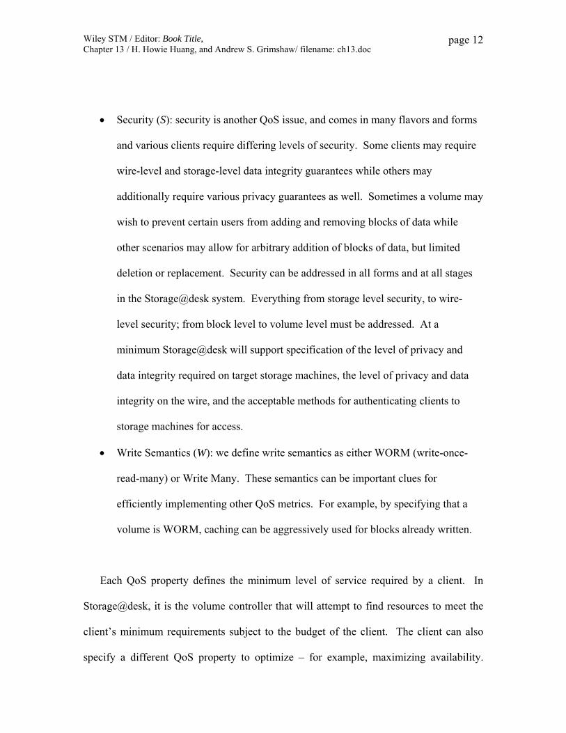
• Security (S): security is another QoS issue, and comes in many flavors and forms
and various clients require differing levels of security. Some clients may require
wire-level and storage-level data integrity guarantees while others may
additionally require various privacy guarantees as well. Sometimes a volume may
wish to prevent certain users from adding and removing blocks of data while
other scenarios may allow for arbitrary addition of blocks of data, but limited
deletion or replacement. Security can be addressed in all forms and at all stages
in the Storage@desk system. Everything from storage level security, to wire-
level security; from block level to volume level must be addressed. At a
minimum Storage@desk will support specification of the level of privacy and
data integrity required on target storage machines, the level of privacy and data
integrity on the wire, and the acceptable methods for authenticating clients to
storage machines for access.
• Write Semantics (W): we define write semantics as either WORM (write-once-
read-many) or Write Many. These semantics can be important clues for
efficiently implementing other QoS metrics. For example, by specifying that a
volume is WORM, caching can be aggressively used for blocks already written.
Each QoS property defines the minimum level of service required by a client. In
Storage@desk, it is the volume controller that will attempt to find resources to meet the
client’s minimum requirements subject to the budget of the client. The client can also
specify a different QoS property to optimize – for example, maximizing availability.

Wiley STM / Editor: Book Title, Chapter 13 / H. Howie Huang, and Andrew S. Grimshaw/ filename: ch13.doc
page 13
Clients will configure Storage@desk volumes with QoS policy documents (similar to
DESL documents) and may submit similar documents at various stages during a
volume’s lifetime for the purposes of providing hints to the system about more immediate
scheduling decisions (such as how much data to pre-fetch into a block, etc.). Example
1Example 1 shows a sample of such a document. Note that the end client may not ever
see a document of this form if proper UI tools are developed which translate more natural
client requirements into requirements the system understands.
<volume id="672362D1-06A6-45db-B4E1-A77D0B3AB4E5"> <name>UVa Volume</name> <owner>CN=Thomas Jefferson 1,[email protected],OU=UVA Standard PKI User,O=University of Virginia,C=US</owner> <availability>99%</availability> <budget>1000</budget> <capacity>524288000 bytes</capacity> <duration>infinite</duration> <reliability>99.9%</reliability> <security> <storage> <privacy-level>encrypted</privacy-level> <integrity-level>checksum</integrity-level> </storage> <on-wire> <privacy-level>encrypted</privacy-level> <integrity-level>checksum</integrity-level> </on-wire>
<authentication-mechanism>X.509</authentication-mechanism> </security>
<performance allocation="50"> <read-write-ratio>2.5</read-write-ratio> <coherence-window>5 minutes</coherence-window> </performance> <optimize>cost</optimize> </volume>

Wiley STM / Editor: Book Title, Chapter 13 / H. Howie Huang, and Andrew S. Grimshaw/ filename: ch13.doc
page 14
Example 1: Illustrative document describing some QoS properties that a volume of
storage might have. We have shown several different QoS properties, persistence,
performance, availability, and integrity. Also included is an optional “allocation” for
each. This indicates the relative importance the user attaches to different QoS elements.
13.4 Storage Market Model
In Storage@desk, competing independent clients or applications “purchase”
storage resources from competing independent machines. In the auction market, storage
machines hold auctions and solicit bids from a number of interested clients. At the
beginning of the auction, each machine will announce the quantity of storage resources
and history data on QoS properties. Because each client may receive bidding invitations
from multiple storage machines, she will independently evaluate them and make a sealed
bid to one machine. A bid includes quantity, and the price. Upon receiving bids, a
storage machine will try to select a client that is willing to offer the highest price.
In the posted-price market, competing independent clients or applications
purchase storage resources from competing independent machines. The model utilizes
pricing agents to help storage providers determine the price for local resources. With the
help of local search algorithms, pricing agents require no direct information of providers
and consumers, which makes this approach very suitable for a grid environment. Thus,

Wiley STM / Editor: Book Title, Chapter 13 / H. Howie Huang, and Andrew S. Grimshaw/ filename: ch13.doc
page 15
pricing agents only need to adjust resource prices periodically based upon locally
observed consumer demand.
In both market models, the consumers are free to use their own strategies to
choose from which provider to purchase. They, however, can’t always get what they
want due to the budget constraints. When two clients have the identical QoS
requirement, the one with larger budget should have a better chance to meet the QoS.
The use of a budget based system provides a mechanism to arbitrate between competing
and likely conflicting clients and also provides a mechanism for system administrators to
assign relative priorities between clients (or at least their purchasing power). We will use
this market approach to produce a storage grid that can 1) achieve a relatively stable
state; 2) fulfil client QoS when adequate budgets are available; and 3) degrades in
accordance with relative budget amounts.
13.4.1 Assumptions
In the Storage@desk market model, we assume that the value, or relative worth, of
a storage resource is ultimately determined by supply and demand. Traditionally, a
market is said to be in equilibrium state when there is a perfect balance of supply and
demand. In grid environment, as is often the case in real life, the balance is difficult to
achieve and maintain because of the existence of unpredictable system dynamics.
Therefore we choose to measure market dynamics by the degree to which the utilizations

Wiley STM / Editor: Book Title, Chapter 13 / H. Howie Huang, and Andrew S. Grimshaw/ filename: ch13.doc
page 16
on storage machines fluctuate. The utilization of a storage machine is defined as the
percentage of used resources. As we will see, when the utilization does not change
widely, neither does the price. Thus, if few changes to resource allocation are needed, we
say the system is in a stable state.
We assume that the storage consumers and providers are self-interested
“individuals” driven by personal goals. Obviously, a storage consumer aims to purchase
storage resources that are affordable within the budget and satisfy the QoS.
13.4.2 Virtual Volumes
Clients create virtual volumes each of which has a particular size and consists of a
number of blocks. A client will need to buy a number of blocks in the market. Each
block represents the capability of storing a fixed amount of data on a specific machine. It
is important to emphasize that we differentiate the blocks in terms of quality. For
instance, some blocks are considered to have better QoS because the underlying
machines are highly available and reliable. While the same quantity of disk storage is
provided, the blocks with better QoS properties should become more expensive for two
reasons. First, it is fair to reward a provider for a better services rendered. Second, it will
help the clients to tell a “good” block from a “bad” one, thus spend the budget efficiently
and have better chance to achieve QoS goals.
For simplicity, we say that the market consists of a finite number S of blocks,
distinguishable in terms of quality, from which a consumer may choose to create a virtual

Wiley STM / Editor: Book Title, Chapter 13 / H. Howie Huang, and Andrew S. Grimshaw/ filename: ch13.doc
page 17
volume. We use RS to denote the resource space. As a volume consists of a number of
blocks, an allocation vector x = [x1, …, xS] can represent the blocks purchased by a
consumer, where x is in RS and a non-negative number xi stands for the amount of the i-th
blocks.
13.4.3 Storage Providers
A storage provider, as a storage machine, sells a number of blocks out of the
available free disk space it has via some allocation policy, such as a fixed amount of
dedicated storage, some percentage of currently unused storage, etc. Each storage
machine is responsible for determining how many raw storage blocks it has to offer, for
how long, and at what price (with the help of a pricing agent). All of the storage
managed by a single storage machine is equivalent so that a storage machine simply has
to determine and advertise the number of blocks available and a single price point for any
of them. However, as we pointed out before, storage resources on two machines are not
necessarily equivalent. For each storage machine, the revenue is calculated as the product
of the price and the number of used blocks. There exists a software agent on each
machine, which is called the auctioning agent in the auction market and the pricing agent
in the posted-price market, respectively.
In the auction market, the auctioning agent will hold the auction for the resources
on the storage machines. When the auction starts, the agent on the i-th machine sends the

Wiley STM / Editor: Book Title, Chapter 13 / H. Howie Huang, and Andrew S. Grimshaw/ filename: ch13.doc
page 18
invitations to the potential interested buyers in the form of (yi, qi), where yi represents the
number of the blocks and qi the history data on the QoS properties. A bid from the j-th
machine can be represented as (xj, pj), where xj represents the number of the blocks the
machine needs and pi the price willing to pay. It is important to note that xj is less than or
equal to yi. When the auction ends, the agent will select the machine with the highest
price and award the requested resources. In case there is a tie, the earliest bid wins. If
there are more resources than what the machine needs, e.g., yi > xj if the j-th machine
wins, the agent will go through the buyer list in the descending order of their bidding
price and repeat the selection process.
In the posted-price market, as each machine wants to maximize the revenue, the
pricing agent will leverage the pricing power to affect the utilization and in turn the
revenue. We will discuss the pricing algorithm in details in Section 13.4.5. We define a
price vector p = [p1, …, pS] to represent the prices of the blocks, where pi is the price of
the i-th blocks. Once a client makes a purchase, this storage service will be rendered by
the storage provider for a predefined period of time. It is the machine’s job to make sure
the blocks solely available to the client.
13.4.4 Storage Consumers
Storage consumers are volume controllers which clients use as their agents. Clients
express their needs to volume controllers in the form of virtual volumes. Each volume is
specified in the form of a QoS vector q = [A, B, C, D, R]. Clients allocate portions of

Wiley STM / Editor: Book Title, Chapter 13 / H. Howie Huang, and Andrew S. Grimshaw/ filename: ch13.doc
page 19
their overall budget to each of their volumes and the volume controllers use this budget to
purchase resources from storage machines. Acting on behalf of clients, volume
controllers agree to buy blocks from storage machines to construct virtual volumes.
Figure 13.2 shows the steps of resource allocation when clients want to create a volume.
1) Storage machines advertise their current price and QoS attributes. 2) Clients specify
QoS and budget constraint. 3) Volume controllers retrieve machine information. 4)
Volume controllers purchase blocks from a number of storage machines, and 5) construct
a storage solution to meet the client-specific QoS criteria. 6) iSCSI servers serve client
requests via iSCSI protocol. 7) Volume controllers monitor service, and 8) inform clients
of up to date status on resource prices and the QoS properties.
Figure 13.2. Logical resource allocation process
The allocation problem can be formalized as follows:
Given the resource space RS and the price vector p = [p1, …, pS], a consumer
would seek an allocation vector x = [x1, …, xS] for a volume with a QoS vector q
= [A, B, C, D, R], which can
4. Create volume
.
.
.3. Purchase blocks
1. Advertise price
2. Retrieve Machine
Info
6. Monitor service
7. Inform status
5. Serve requests
Client
Database
Volume Controller
iSCSI Server 5. Serve requests
#, $ StorageMachine
Pricing Agent
#, $ StorageMachine
Pricing Agent
Wiley STM / Editor: Book Title, Chapter 13 / H. Howie Huang, and Andrew S. Grimshaw/ filename: ch13.doc
page 20
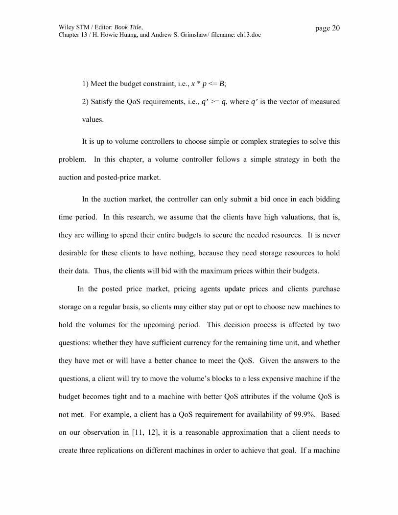
1) Meet the budget constraint, i.e., x * p <= B;
2) Satisfy the QoS requirements, i.e., q’ >= q, where q’ is the vector of measured
values.
It is up to volume controllers to choose simple or complex strategies to solve this
problem. In this chapter, a volume controller follows a simple strategy in both the
auction and posted-price market.
In the auction market, the controller can only submit a bid once in each bidding
time period. In this research, we assume that the clients have high valuations, that is,
they are willing to spend their entire budgets to secure the needed resources. It is never
desirable for these clients to have nothing, because they need storage resources to hold
their data. Thus, the clients will bid with the maximum prices within their budgets.
In the posted price market, pricing agents update prices and clients purchase
storage on a regular basis, so clients may either stay put or opt to choose new machines to
hold the volumes for the upcoming period. This decision process is affected by two
questions: whether they have sufficient currency for the remaining time unit, and whether
they have met or will have a better chance to meet the QoS. Given the answers to the
questions, a client will try to move the volume’s blocks to a less expensive machine if the
budget becomes tight and to a machine with better QoS attributes if the volume QoS is
not met. For example, a client has a QoS requirement for availability of 99.9%. Based
on our observation in [11, 12], it is a reasonable approximation that a client needs to
create three replications on different machines in order to achieve that goal. If a machine
Wiley STM / Editor: Book Title, Chapter 13 / H. Howie Huang, and Andrew S. Grimshaw/ filename: ch13.doc
page 21
becomes less reliable, it may become necessary for the client to move the replica to a
more reliable machine. If the budget becomes insufficient, the client may need to move a
replica to a less expensive machine or reduce the number of replicas. It is possible that a
client does not have sufficient budget to compete for “good” resources. As a result, the
client has to make the trade-offs between various QoS criteria – including trade-offs
between the amount of space one can get and the quality of the service one receives.
13.4.5 Storage Resource Pricing
At its heart, Storage@desk is a storage scavenging system that must deal with
machines that are typically under the direct control of desktop users. Those machines
often exist in an environment that is highly unstable and dynamic. This implies that those
machines experience dramatic changes in load, disk usage, connectivity, uptime, etc.
depending on the whims of the user sitting at the console. Additionally, administrative
domains may enforce policy leading to large, coordinated downtimes and periods of
unavailability. However, the chaotic nature of this environment should not prevent us
from delivering reasonable level of QoS. Indeed, we believe that local search pricing
agents will hold the most promise for Storage@desk. A local search pricing agent
requires no assumption or knowledge of other providers and of the consumer population.
Such an agent utilizes a local search algorithm that periodically adjusts the resource price
based upon the demands observed in the previous and current time windows.

Wiley STM / Editor: Book Title, Chapter 13 / H. Howie Huang, and Andrew S. Grimshaw/ filename: ch13.doc
page 22
We choose to employ two classes of local search algorithms, greedy algorithm and
derivative-following (DF) algorithms. A greedy pricing agent starts with a pre-defined
price and makes small changes (increase or decrease) as long as the demand increases.
Such an agent stops changing the price when it cannot see any improvement in demand.
At this point, it is considered that a good price is found. Ideally, the price is close to the
optimal value. The price moves in a small step δ, which is chosen randomly from a
specified range; in the simulation we use a uniformly random distribution between 10%
and 30%. We have found a random increment helps reduce the negative impacts from
unpredicted dynamics in a distributed environment. Algorithm 1 lists the pseudocode of
the greedy algorithm.
In contrast, a derivative-following pricing agent will not terminate the search when
there is no increase in demand. Rather, a DF agent will reverse the search direction at that
point. A DF agent starts with a pre-defined price and changes the price in the same
direction at each observation window until the most recent demand is observed to
Algorithm 1: Greedy Pricing Algorithm
Set direction as UP or DOWN based on initial observations FOR each time interval ti (i >=2) DO
IF di >= di-1 THEN IF direction == UP THEN
pi = pi-1 * (1 + δ) ELSE pi = pi-1 * (1 - δ) END IF ELSE RETURN the price pi END IF END FOR

Wiley STM / Editor: Book Title, Chapter 13 / H. Howie Huang, and Andrew S. Grimshaw/ filename: ch13.doc
page 23
decrease from the demand in the previous window. In that case, the agent reverses the
search direction and begins to make price changes in the other direction. When the
demand again decreases the price movement will be reversed again. Therefore, the agent
is able to track the changes in the observed demand and react fairly quickly to reverse the
undesirable trend. In addition, it is very intuitive and requires only local knowledge. The
latter makes it possible to develop a highly efficient solution in a grid, which involves a
large number of distributed machines. Algorithm 2 lists the pseudocode of the
derivative-following algorithm.
In conclusion, our market-based model has three advantages. First, a storage
machine is only required to know the local demand. There is no need for a storage
machine to know prices from others, although they may compete for consumers. Nor
does a storage machine need to know demands from all consumers. Second, a storage
machine is allowed to leverage independent pricing power to compete for positions in the
market. Thus, rather than one price fits all, the market recognizes the quality differences
between storage resources and enables prices to reflect those differences. Third, with the
Algorithm 2: Derivative-Following Pricing Algorithm
FOR each time interval, ti DO IF di > di-1 THEN
pi = pi-1 * (1 + δ) ELSE IF di < di-1 THEN pi = pi-1 * (1 - δ) ELSE pi = pi-1 END IF END FOR

Wiley STM / Editor: Book Title, Chapter 13 / H. Howie Huang, and Andrew S. Grimshaw/ filename: ch13.doc
page 24
feedback price signals, a client is encouraged to make trade-offs among many QoS
attributes and compose a service that maximizes QoS under a specific budget.
13.5 Evaluations
Using our market model, we want to provide two things with respect to availability
and resource allocation. First, the overall resource allocation system and pricing
performance in the system can be stable. Second, when resources are available, the
resource allocation mechanism must perform efficiently and effectively – meaning that
volume controllers make the proper decisions and can purchase the proper resources to
meet their availability goals. Additionally, the resource allocation process should
degrade such that it favors those who have allocated higher budgets to their storage when
all other things are equal.
To evaluate our model, we construct a trace-driven simulation. In this simulation,
we choose to study volume availability to demonstrate the effectiveness of our market
model. We simulate our model using trace data, which we collected from 729 public
machines in the classrooms, libraries, and laboratories at the University of Virginia. An
analysis of this data has been published as a feasibility study of Storage@desk [9].
During a time period of three months in 2005, these public machines send to a central
database a snapshot for each five-minute interval that contains statistics such as free disk
space, CPU utilization, memory usage, etc. Figure 13.3 shows the number of available
machines for each five-minute interval. Around 700 machines were reachable most of

Wiley STM / Editor: Book Title, Chapter 13 / H. Howie Huang, and Andrew S. Grimshaw/ filename: ch13.doc
page 25
the time. There were several events where large number of machines went down due to
network partition, power outage, and scheduled maintenance, etc., which are displayed as
the downward spikes in the figure.
Figure 13.4 shows the number of machines categorized by their availabilities in
terms of nines over the 10-week span. We use three-nine machines to represent the
machine group whose availability is greater than 99.9%, two-nine machines for
availability greater than 99%, and one-nine machines for availability greater than 90%.
The majority of the machines had an availability of 2 nines or 3 nines. Although more
than 500 machines started with 3 nines at the first week, their availabilities gradually
decreased as the time went by. This was expected given the unreliable nature of machine
usage on these desktops. At the same time, the number of one-nine and two-nine
machines increased significantly. The population of zero-nine machines remained steady
for 10 weeks. In the end, there were about 60 three-nine machines, 200 two-nine
machines, 400 one-nine machines, and 75 zero-nine machines.

Wiley STM / Editor: Book Title, Chapter 13 / H. Howie Huang, and Andrew S. Grimshaw/ filename: ch13.doc
page 26
Figure 13.3. Number of available machines Figure 13.4. Machine counts by availability
Each volume is assigned with a budget of 100 (low budget), 200 (medium budget)
and 300 (high budget), in a random, uniform distributed fashion. Also, a volume is
randomly given an availability requirement of 1 nine, 2 nines and 3 nines. This
assignment creates a good mix of various budgets and availabilities among the volumes.
In our simulation, we assume that each volume consists of one block and each machine
has 10 blocks available for Storage@desk, so each machine can hold up to 10 volumes.
Under a pre-defined budget and availability requirement, each client creates one
volume by purchasing blocks and makes a number of replicas for the volume in order to
satisfy the availability requirement. The number of replicas a client tries to make is
determined by how many nines the client desires. For example, a client with a
requirement of 3 nines will make three replicas of the volume. As we pointed out earlier,
this is a reasonable choice given the fact that the majority of the machines have an
availability of 90% or higher. We make sure that one machine will not hold two replicas
of the same volume, so a client will distribute three copies on three different machines.
From the trace, we know the status of each machine, in other words, whether the
machine is available, at every five-minute interval. A volume is available as long as
there is at least one replica accessible, otherwise it is unavailable. Thus, we can easily
obtain MTTF and MTTR for each volume, and compute its availability.
We simulate our model in two market settings, the over-supply and under-supply
cases. Note that 729 storage machines can hold 7,290 volumes, which is the supply in

Wiley STM / Editor: Book Title, Chapter 13 / H. Howie Huang, and Andrew S. Grimshaw/ filename: ch13.doc
page 27
the market. In the over-supply case, there are 3,500 clients, i.e., 3,500 volumes in the
system, which consume 95% of supply if each volume makes 2 copies on average. Due
to the budget constraints on some volumes, the actual consumption is much lower, about
76% at the beginning of the simulation as shown in Figure 13.7 (a). In the under-supply
case, there are 4,500 clients demanding 120% of supply.
In the auction market, each storage machine will randomly solicit bids from 60
clients. In the posted-price market, storage machines set the initial price as Priceinitial =
(budget / demand) / duration, where budget is the total amount of currency in the system
at the beginning of the simulation, demand is the number of blocks needed by all the
clients, and duration is the number of weeks in the simulation (10 weeks). We
intentionally lower the initial price by 10% to create an initial leeway for customers with
a tight budget.
.
13.5.1 Price and Allocation Stability
In this section we study the mean price and mean utilization distributions under two
demand scenarios. Figure 13.5 show the mean price distribution in the auction market
model for the oversupply case (a) and the under-supply case (b). In both cases, while the
prices increase slowly from week 2 to week 9 for machines have less than 3 nines, they
jump in the end of the simulation. The weekly increase is significantly larger for three-
nine machines. This is caused by the fact that the low-budget clients who do not have

Wiley STM / Editor: Book Title, Chapter 13 / H. Howie Huang, and Andrew S. Grimshaw/ filename: ch13.doc
page 28
sufficient funds to win bids in the beginning of the simulation are able to afford good-
quality machines later on. As we will see later, the posted-price market model can avoid
this problem, as low-budget clients manages to purchase “cheap” resources from low-
quality machines.
a) Over-supply case (b) Under-supply case
Figure 13.5. Auction - mean price distribution for 10 weeks
Now we will first look at how greedy pricing affects the price for the time period of
10 weeks. For the over-supply case (Figure 13.6 (a)), all machines start with the same
initial price of 9.17, but begin to diverge in week 3. As the simulation continues, the
clients begin to assess their volumes and resource allocations, and take appropriate
actions based on perceived availabilities and the remaining budget. Subsequently, the
machines with higher number of nines will see more demand from clients, while those
with lower nines experience diminishing demands. So, machines with 2 or 3 nines begin
to ask a higher price for its storage resources, while machines with 0 or 1 nine begin to

Wiley STM / Editor: Book Title, Chapter 13 / H. Howie Huang, and Andrew S. Grimshaw/ filename: ch13.doc
page 29
ask for a lower price. As a result, two-nine machines have a price of about 7% higher
than zero-nine machines. Since there are more two-nine machines, they have a better
chance seeing higher demand than three-nine machines and thus have a higher price in
the end of the simulation. For the under-supply case (Figure 13.6 (b)), the prices also
diverge, but to a much smaller degree. The machine groups with lower nines will not
experience a significant drop of client demands, since the demand exceeds the total
supply in the system. The clients become less quality sensitive, and pay more attention to
the quantity. As a result, machines with more than two nine have a very close mean
price, so do machines with zero or one nine. And the price gap between two-nine
machines and zero-nine machines becomes larger, about 15%, at Week 10.
Figure 13.7 illustrates the mean price distribution for derivative-following pricing
for each of the four availability classes (base on the number of nines) over the 10-week
study. For the over-supply case (Figure 13.7 (a)), all machines also start with the same
initial price of 9.17, and begin to diverge in week 3 based on their availabilities. The
price changes continue till week 8, where the prices reach a relatively stable level. At
week 10, zero-nine machines have the lowest mean price of 7.55, while three-nine
machines have the highest mean price of 10.60, or 40% higher. This gap is much bigger
than the one when using greedy pricing. Also this time, three-nine machines have a
slightly higher price than two-nine machines, reflecting the order of their availability.
For the under-supply case (Figure 13.7 (b)), similar to what happens in greedy pricing,
the prices diverges to a smaller degree. Machines with more than one nine have a very
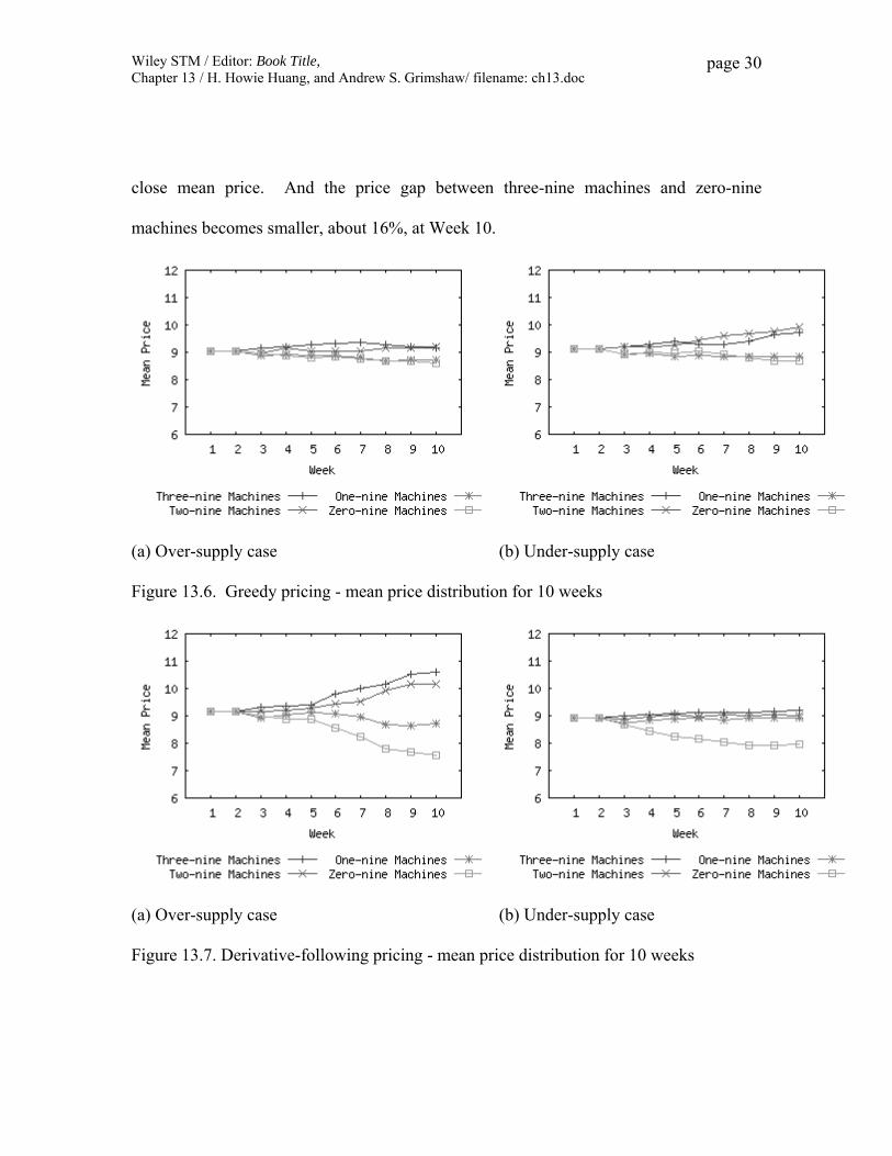
Wiley STM / Editor: Book Title, Chapter 13 / H. Howie Huang, and Andrew S. Grimshaw/ filename: ch13.doc
page 30
close mean price. And the price gap between three-nine machines and zero-nine
machines becomes smaller, about 16%, at Week 10.
(a) Over-supply case (b) Under-supply case
Figure 13.6. Greedy pricing - mean price distribution for 10 weeks
(a) Over-supply case (b) Under-supply case
Figure 13.7. Derivative-following pricing - mean price distribution for 10 weeks

Wiley STM / Editor: Book Title, Chapter 13 / H. Howie Huang, and Andrew S. Grimshaw/ filename: ch13.doc
page 31
The clients try to shy away from low available machines and pursue machines with
high availability if the budget allows. Figure13.8 show the mean utilizations in the
auction market. In the auction market, the three-nine machines at week 10 have a mean
utilization of 86% and 97% in the over-supply and under-supply case, respectively. In
contrast, the zero-nine machines at the week 10 have a mean utilization of 50% and 58%
in the over-supply and under-supply case, respectively. The utilization in the posted-
price market is higher as shown in Figure 13.9, because in this case clients can always get
what they intend to purchase. In contrast, the clients who do not win bids in the auction
market will not get another chance to purchase resources until next week. As both
pricing algorithms have similar effects on resource utilization, we choose to only present
derivative-following pricing here. For the over-supply case (Figure 13.9 (a)), three-nine
machines start with 76% utilization and become close to fully utilized at week 8; on the
other hand, zero-nine machines see the utilization decreases gradually till around 40% at
week 7. For the under-supply case (Figure 13.9 (b)), machines with 2 or 3 nines quickly
become fully utilized. The utilization on zero-nine machines and one-nine machines
remains 82% and 94%, respectively, due to the overwhelming demand in the system.

Wiley STM / Editor: Book Title, Chapter 13 / H. Howie Huang, and Andrew S. Grimshaw/ filename: ch13.doc
page 32
(a) Over-supply case (b) Under-supply case
Figure 13.8. Auction - mean utilization distribution for 10 weeks
(a) Over-supply case (b) Under-supply case
Figure 13.9. Derivative-following pricing - mean utilization distribution for 10 weeks
Figure 13.10 and 13.11 present volume migration rates in10 weeks for greedy
pricing and derivative-following pricing respectively. We can see that, for both pricing
algorithms, when volumes have a higher budget, less than 10% of them need to move
their replicas at each week to improve their availabilities. Volumes with low budget

Wiley STM / Editor: Book Title, Chapter 13 / H. Howie Huang, and Andrew S. Grimshaw/ filename: ch13.doc
page 33
migrant more frequently, because they have to consistently search for affordable
resources as a result of competitions. For the under-supply case, very few volumes
migrate due to the limited supply of resources.
(a) Over-supply case (b) Under-supply case
Figure 13.10. Greedy pricing - mean utilization distribution for 10 weeks
(a) Over-supply case (b) Under-supply case
Figure 13.11. Derivative-following pricing - mean utilization distribution for 10 weeks

Wiley STM / Editor: Book Title, Chapter 13 / H. Howie Huang, and Andrew S. Grimshaw/ filename: ch13.doc
page 34
For derivative-following pricing, 2,325 volumes, or 66.4%, do not migrate at all in
the over-supply case, and 2,858 volumes, or 81.9%, migrate less than twice. In other
words, the majority of the volumes are able to quickly find resources that can meet their
availability requirements. In total the volumes perform 3,601 migrations over 10 weeks,
of which 63% come from the low budget volume, 21% from the medium budget volume,
and 16% from the high budget volume. This is expected because, while the high budget
volumes can still afford good resources, some low budget volumes are forced to move as
the price pressure increases. In the under-supply case, with limited supply, the market
has no much room for the volumes to move around. As a result, 3,896 volumes, or
86.6%, do not migrate once, while 4,396 volumes, or 97.7%, migrate less than twice.
Among 1,045 migrations from all the volumes, 64% come from the low budget volume,
20% from the medium budget volume, and 16% from the high budget volume. These
numbers are quite close to those from the over-supply case. It indicates that the volumes
with higher budgets do have a better chance to quickly find reliable resources and meet
the availability. Therefore, we consider, in the over-supply case, the system becomes
stable when the machines reach steady utilizations at week 8 and the clients with
sufficient budgets complete the volume migrations. In the under-supply case, the large
demand has already confined the market movements to a smaller window, thus the
system becomes stable rather quickly when the machines remain steady utilizations since
week 4.

Wiley STM / Editor: Book Title, Chapter 13 / H. Howie Huang, and Andrew S. Grimshaw/ filename: ch13.doc
page 35
13.5.2 Meet Availability Goals and Adherence to Budgeted Priorities
For each client, the key is to meet the availability goal under the budget constraint.
It is expected, to a high probability, a volume should be able to meet a relatively lower
availability for a wide range of the budgets, because in this case a volume only needs a
small number of replicas that can be done with a small budget. On the other hand, when
a volume needs a high availability, the volume has to purchase a large quantity of storage
resources for replicas. This can be difficult when the budget is limited. Therefore, there
exists a contention for storage resources and the budget constraint will eventually affect
the probability of a volume can meet the availability. As the posted-price market
produces more stable prices and utilizations than the auction market, we will only show
the results from the former in the section. In the posted-price market, both pricing
algorithms can prioritize clients based on their budgets, and we will only present the
results from derivative-following algorithm here. Figure 13.12 and 13.13 show the
percentage of volumes that satisfy the availability of 1 nine and 3 nines, respectively. In
each figure, (a) illustrates the over-supply case and (b) presents the under-supply case.
From Figure 13.12, we can see that the budget plays a small role for one-nine volumes.
In the over-supply case, 88% of high budget volumes meet the 1 nine availability at week
10, while 87% of low budget volumes do. This small difference becomes even smaller in
the under-supply case. It indicates that low budget is sufficient for a volume that needs a
low availability.

Wiley STM / Editor: Book Title, Chapter 13 / H. Howie Huang, and Andrew S. Grimshaw/ filename: ch13.doc
page 36
(a) Over-supply case (b) Under-supply case
Figure 13.12. Percentage of one-nine volumes that satisfy the availability
(a) Over-supply case (b) Under-supply case
Figure 13.13. Percentage of three-nine volumes that satisfy the availability
The situation changes when a volume has an availability of 2 nines. The chance for
a low budget volume has 2 nines availability decreases from 87% at week 1 to 36% at
week 10 in the over-supply case and from 87% to 33% in the under-supply case. In

Wiley STM / Editor: Book Title, Chapter 13 / H. Howie Huang, and Andrew S. Grimshaw/ filename: ch13.doc
page 37
comparison, above 90% of the medium and high budget volumes still have a good chance
to meet the availability requirements. In this case, the budget draws a clear distinction
between low budget volumes and higher budget volumes, while medium and high budget
still can be considered equivalent. The latter can no longer hold true as shown in Figure
13.11 when the volumes demands an availability of 3 nines, where each volume needs to
purchase storage for three replicas. While about 92% of high budget volumes meet the
goal at week 10, the percentage for medium budget volumes and low budget volumes
drop to 70% and 8% in the over-supply case, and 70% and 7% in the under-supply case.
In summary, the system is able to achieve, in both cases, a partial ordering of client QoS
fulfilment matching client budget ordering, which clearly serves the purpose of the
budget constraint. This should encourage clients to make trade-offs between resource
price and various QoS attributes.
13.6 Future Research Directions
This study enhances our understanding of how market approach helps with storage
resource allocation in a new storage grid. However, much remains to be learned about
the agent behavior and market model in Storage@desk.
• We will take computing and network resources into considerations to give our
model a higher level of realism. This will inevitably introduce new research
challenges. When a client purchases various resources from multiple providers, it

Wiley STM / Editor: Book Title, Chapter 13 / H. Howie Huang, and Andrew S. Grimshaw/ filename: ch13.doc
page 38
needs to carefully make a purchase plan ahead of time in order to coordinate the
consumption of different resources at the desirable time.
• We will explore new QoS properties, e.g., security and performance, and support
them in our market model. Their impacts on resource management can be two-
fold. First, like the previous problem of multiple resource purchase, a client need
to make a good plan in order to simultaneously achieve multiple QoS properties.
It may come to a time when it is not possible to achieve all desired QoS
properties. At that time the client has to prioritize one or more most important
properties. Second, we plan to research other possible pricing algorithms, e.g.,
based on genetic algorithm or ant colony algorithm.
• We will introduce the concept of penalty to the market. A penalty will be
assessed when a resource provider cannot meet its pre-specified QoS level. For
example, for a resource provider advertising an available of 99.9%, it needs to pay
a certain amount of penalty for the time periods that it did not provide a three-nine
service. This will provide an incentive for providers to honestly announce the
quality of their services.
13.7 Conclusion
In this chapter, we present a market-based resource allocation model for
Storage@desk, a new storage grid where software agents determine local prices for
resource providers based on the derivative-following algorithm. We describe both the

Wiley STM / Editor: Book Title, Chapter 13 / H. Howie Huang, and Andrew S. Grimshaw/ filename: ch13.doc
page 39
auction market model and the posted-price market model in the Storage@desk
architecture. We use a trace-based simulation to evaluate both models and show that the
posted-price market model is able to produce a more stable market with higher
utilization.
In the posted-price market, once the price, quantity, and quality of storage resources
are advertised, storage consumers can choose from which providers to buy, and how
many. With the help of the volume controller, a client can make trade-offs among many
QoS attributes and compose a service that achieves the desirable QoS under a specific
budget. A good resource allocation can be achieved by the cooperation from two sides:
providers adjust prices for their resources in accordance with the demand they
experience, while consumers adjust their allocation as reacts to the QoS experienced and
the price changes based on the amount of currency left in the budget.
.
Acknowledgment This chapter is a substantial extension of a paper published in IEEE/WIC/ACM
International Conference on Web Intelligence (WI) in November 2007.
References

Wiley STM / Editor: Book Title, Chapter 13 / H. Howie Huang, and Andrew S. Grimshaw/ filename: ch13.doc
page 40
1. C.A. Waldspurger, T. Hogg, B.A. Huberman, J.O. Kephart, and W.S. Stornetta, Spawn: A Distributed Computational Economy, IEEE Transaction on Software Engineering, 18(2), pp. 103-117, 1992.
2. K. Lai, L. Rasmusson, E. Adar, S. Sorkin, L. Zhang, and B.A. Huberman, Tycoon: an Implementation of a Distributed Market-Based Resource Allocation System, Multiagen Grid System, 1(3), pp. 169-182, 2005.
3. A. AuYoung, B. Chun, A. Snoeren, and A. Vahdat, Resource allocation in federated distributed computing infrastructures, in Proceedings of the 1st Workshop on Operating System and Architectural Support for the Ondemand IT InfraStructure, 2004.
4. B. Chun and D. Culler, Market-based Proportional Resource Sharing for Clusters, in Technical Report CSD-1092, University of California at Berkeley, Computer Science Division, January 2000.
5. R. Wolski, J. Plank, J. Brevik, and T. Bryan, G-Commerce: Market Formulations Controlling Resource Allocation on the Computational Grid, in Proceedings of International Parallel and Distributed Processing Symposium, San Francisco, California, USA, April 23-27, 2001.
6. M. Placek and R. Buyya, Storage Exchange: A Global Trading Platform for Storage Services, in Proceedings of the 12th International European Parallel Computing Conference, Dresden, Germany, Aug. 29-Sept 1, 2006.
7. T. Eymann, M. Reinicke, O. Ardaiz, P. Artigas, F. Freitag, and L. Navarro, Decentralized resource allocation in application layer networks, in Proceedings of the 3rd International Symposium on Cluster Computing and the Grid, Tokyo, Japan, May 12-15, 2003.
8. P. Padala, C. Harrison, N. Pelfort, E. Jansen, M.P. Frank, and C. Chokkareddy, OCEAN: the open computation exchange and arbitration network, a market approach to meta computing, in Proceedings of International Symposium on Parallel and Distributed Computing, Ljubljana, Slovenia, 2003.
9. H.H. Huang, J.F. Karpovic, and A.S. Grimshaw, A Feasibility Study of a Virtual Storage System for Large Organizations, in 1st IEEE/ACM International Workshop on Virtualization Technologies in Distributed Computing (held in conjunction with SC06), Tampa, Florida, USA, November 17, 2006.
10. IETF. Internet Small Computer Systems Interface (iSCSI), http://www.ietf.org/rfc/rfc3720.txt, April 2004.
11. Jakka Sairamesh and J.O. Kephart, Price Dynamics of Vertically Differentiated Information Markets, in Proceedings of First International Conference on Information and Computation Economies, Charleston, South Carolina, USA, 1998.
12. Jeffrey O. Kephart, James E. Hanson, and A.R. Greenwald, Dynamic Pricing by Software Agents, Computer Networks, 32(6), pp. 731-752, 2000.