Resource planning and resource allocation in the

•^''"':'=-l'«:|??lS SCHOOL

RESOURCE PLANNING AND RESOURCE ALLOCATIONIN THE CONSTRUCTION INDUSTRY

BY

CHARLES E. MENDOZA

A REPORT PRESENTED TO THE GRADUATE COMMITTEEOF THE DEPARTMENT OF CIVIL ENGINEERING IN

PARTIAL FULFILLMENT OF THE REQUIREMENTSFOR THE DEGREE OF MASTERS OF ENGINEERING

UNIVERSITY OF FLORIDA

SUMMER 1995

DUDLEY KNOX LIBRARYNAVAL POSTGRADUATE SCHOOLIWOWTCREY CA 93943-5101

To my wife, Adelaida, without whose support, love, inspiration and

encouragement I would never have written this report. I also would like give special

thanks to my parents Juan and Ana Mendoza, my brothers, and sisters for all of their

love, and support they provided me throughout my graduate career here at the

University of Florida.

ACKNOWLEDGEMENTS

I would like to extend my deep gratittude to Dr. Charles Glagola, mysupervisory committee chairman, for his guidance and dedicated support that made this

report possible. I am sincerely appreciative of Dr. Zohar Herbsman and Dr. Ralph

D. Ellis for serving on my supervisory committee.

1

HI

Table of contents

Introduction 1

Chapter One - Resource Planning

1 .

1

Introduction 3

1 .2 Human Resources 3

1.2.1 Theoretical Personnel Loading Curves 4

1.2.2 Practical Personnel Loading Curves 6

1.3 Planning the Construction Project Personnel 8

1.3.1 Planning Field and Staff Personnel 12

1.3.2 Construction Subcontracting 13

1 .4 Construction Material Resources Planning 14

1.4.1 Long Delivery Materials 15

1.4.2 Special Materials and Alloys 16

1 .4.3 Common Materials in Short Supply 17

1.4.4 Services and Systems 17

1.4.5 Transportation Systems 18

1.5 Summary 18

Chapter Two - Resource Handling

2.

1

Introduction 20

2.2 An Example 21

2.3 Limited Resources 25

2.4 Resource Leveling 26

2.4.

1

Single Resource 26

2.4.2 Several Resources 29

Chapter Three - Resource Leveling

3 .

1

Introduction 31

3.2 Leveling the Work Force 31

3.3 Leveling Procedure 32

IV

3.4 Smoothing Resources 33

3.4.1 Resource Histograms 34

3.4.2 Total Effort and Average Crew Sizes 35

3.4.3 Smoothing the Daily Crew Allocations 35

3.5 Stretching out a Task 39

3.6 The Technique: Steps for Resource Leveling 40

3.6.1 Smoothing More than One Resource at a Time 41

3.6.2 Checking your Work: Bookeeping Checks 41

3.7 Summary 43

Chapter Four - Resource Constrained Scheduling

4.

1

Introduction 44

4.2 Heuristics Methods 44

4.2.

1

An example 46

4.2.2 Heuristics Techniques 50

4.3 Optimizing Methods 52

4.3.1 Mathematical Programing 53

4.4 Multi-project Scheduling and Resource Allocation 53

4.5 Summary 55

Chapter Five - Computer Application in Resource Leveling

5 .

1

Introduction 57

5.2 Allocating Resources in Primavera Ver. 1.1a for Windows ....57

5.2.1 Defining a Resource Plan 57

5.2.1.1 Assigning Resources 58

5.2.1.2 Driving Resources 59

5.2.1.3 Setting Resource Limits 60

5.2.1.4 How to Create a Resource Profile 61

5.2.1.5 Resource Tables 62

5.2.2 Refining the Resource Plan 63

5.2.2.1 Adjusting the Resource Distribution 63

5.2.2.2 Distribute Resources Non-linearly 64

5.2.2.3 Leveling Resources 65

5.3 Summary 68

Conclusion 69

References 71

Bibliography 74

VI

INTRODUCTION

Today, construction projects are more complex than ever before. Thousand of

tasks must be precisely controlled if a project is to run smoothly, on time, and in budget.

The completion of a construction project requires the judicious scheduling and allocation

of available resources. Manpower, equipment, and materials are important project

resources that require close management attention. The supply and availability of these

resources can seldom be taken for granted because of seasonal shortages, labor disputes,

equipment breakdowns, competing demands, delayed deliveries, and a host of associated

uncertainties. Nevertheless, if time schedules and cost budgets are to be met, the work

must be supply with the necessary workers, equipment, and materials when and as they

are needed on the job site.

The basic objective of resource planning and resource allocation is to supply and

support the field operations so that established time objectives can be met and costs can be

kept within the construction budget^ It is the responsibility of the project manager to

identify and schedule future job needs so that most efficient employment is made of the

resources available. The project manager must determine long-range resource

requirements for general planning and short term resources for detailed planning. He must

establish which resources will be needed, when they must be on site, and the quantities

required. The project plan and schedule may have to be modified to accommodate or

work around supply problems.

The term resource allocation is used in the case where required resources are

assigned such that available resources are not exceeded. Resource leveling is an attempt

to project activities in a manner that will improve productivity and efficiency.

This report will present an overview on resource planning and resource leveling.

Chapter 1 will will describe resource planning and explain theoretical personnel loading

curves and practical personnel loading curves, and the planning of the construction

project personnel. Chapter 2 will give an introduction on how to handle resources.

Chapter 3 will cover resource leveling and indicate how we can level the workforce.

Chapter 4 will describe resource constrained scheduling. Chapter 5 will describe the use

of computer applications in resource allocation and resource leveling. This chapter will

concentrate on how to use the resource leveling in Primavera project planner software

application.

CHAPTER 1

RESOURCE PLANNING

1.1 Introduction

Resource planning cannot be accomplished without four essential resources

necessary to accomplish the given scope of work: materials, people, equipment, and time.

If the project plan and schedule are to be achieved, it is necessary to assure that the

required material, labor, and equipment will be available when needed in the require

quantities^.

Although the resource planning phase is very inportant, many projects suffer

avoidable delays from inadequate resource planning and control. For example, large

projects get delays when a certain material is not delivered on time.

In resource planning, we need to identify the quantities of resources required to

accomplish the work and schedule these resources over the time of the project.

1.2 Human Resources Planning

Human resources for construction planning breaks down into three major

categories as follows:

Home office personnel

Construction personnel (field supervision and labor)

Construction subcontractors

•

•

Effectively manning the world's construction projects makes the construction

contractor's personnel department a key to successful contracting. Anything the

construction managers can do to facilitate staffing their projects such as personnel

planning will make their personnel departments' work easier and more effective.

1.2.1 Theoretical Personnel Loading Curves

The simplest form of a personnel loading curves is a trapezoid, as shown in figure

1.1^. The curves plot personnel required versus the scheduled time to accomplish the

work. Actually the most efficient way to staff a project would be to immediately staff the

average number of people required on day one, continue to the end ofthe work, then drop

to zero. The average number of people can be derived by dividing the total hours by the

total calendar time, and it is shown graphically by the solid horizontal line in figure 1.1.

We know that such ideal personnel loading is not feasible for many reasons, such

as not having the site ready, not having all of the materials and equipment available, and

not having enough places for the people to work. Because we have to start from zero and

assign people gradually, the next most efficient theoretical personnel loading curve is the

trapezoid. It has a uniform buildup, a level peak, and a uniform builddown. In actual

practice loading curves take the shape of a bell curve as shown in figure 1.1. Because the

bell curve tends to fall inside the trapezoid at the start and the finish, its peak must extend

above the peak of the theoretical curve to account for the lost hours. The area under the

curve is a value that is set by the total labor hours estimated to perform the work. A

good rule of thumb to remember is that the bell curve peak usually exceeds the average

personnel loading curve line by about 20 to 30 percent'*. This ratio allows you

^ 50

S 40

w« 30Ph

"S 20

H 10

Average.Loading

/ / \ \/

/ \Unit Calendar Time

Reproducefrom: Project Resource Planning

Figure J.J Theoretical Personnel Loading Curve

to make an approximation of peak craft personnel requirements as soon as the personnel

estimate has been completed.

The elapsed time for construction execution runs longer than shown on the

theoretical curves, so it's possible to get multiple peaks in certain crafts, as shown in

figure 1.4.

1.2.2 Practical Personnel Loading Curves

So far, I have discussed theoretical curves, but we need to look at some more

likely loading situations that are useful in the practical planning of our human resources.

In figure 1.2^ I have shown the theoretically ideal bell curve as a dashed line, and the

50

^ 40

30

(t> 20

10

Front Loaded Normal Loaded

/ X.// "N • - *

/

/ ^V* \ Back

Loaded

// \ \

/ /\

/

/ #

V

i^—

\\ *\ t

\ %

\ »

Calendar Time


Figure 1.2 Practical Personnel Loading Curves

forward and backward loaded curves as other dash lines also. The latter two result when

the personnel loading curves occur earlier or later than planned on a project.

The significance of these conditions becomes apparent when we look at the set of

"S" curves resulting from plotting percent of hours expended versus scheduled time as

shown in figure 1.3.^

The "S" curve for the ideally loaded project has a gradual start and finish, which

indicates smooth starting and finishing conditions. The forward loaded curve shows a

Normal Loaded100

T3 ^^^'^''''^^^

/

a> ^^^^ \^ y^

M ^0 Front Loaded x / /"Hh \ X^ /

1 60 \/ / /U y / /^*N M ^v / / / Backg 40 / / / Loadedo ^r y/ o;-H ^^ y^ ^

eiH 20 yy ^„^-'^~'

Calendar Time


Figure 1.3 "S" curvesfrom Bell Curves

rapid project start up and an even more gradual than normal phaseout at the end. The

backward-loaded project indicates a more relaxed start and a very steep finish slope on the

"S" curve. The steep finish leads to such problems as inefficient use of personnel and

overrunning the budget. The inefficiency results from having too many people working

on only a few remaining tasks.

Normally, personnel cannot be phase off the job so quickly, which means the

project will overrun the budget. The simple lesson to be learn here is that front loaded

projects may slip to a normally loaded mode and still finish on time. There is little hope

that backward-loaded will finish on time. Any slippage during execution further

aggravates the phase-out problems and makes the project finish still later and more over

the budget than planned.

Construction managers must remember, however, that front loaded projects do

not happen just by drawing only the personnel loading curves that way. All necessary

start-up requirements of design documents, facilities, personnel, and materials and

equipment must be available to support an early labor pool.

1.3 Planning the Construction Project Personnel

Personnel planning for the field involves detailed craft loading curves and the field

supervisory team. When planning for manpower, we should also consider the home

office support personnel since they play an important role in the project effort. Because

their numbers are usually relatively small, loading curves are not practical. In most

projects, the home office personnel are not under the direct administration of the

i

construction manager. However, it is important to keep track of their project activities if

they are charging time to the CM's project budget.

To estimate the total project personnel distribution for the craft labor, it is a good

idea to plot a curve for each major craft to be used in the construction. A typical example

of such a plot is shown in Figure 1.4^, which is actually a composite of all crafts required

to build a process type facility.

700 Carpenter----- Pipefitters, Welders, Instruments

_^" .^v ^vMiUrights A

600 ...—..- Electricians | \ll-/\l-l\X7/^»-lrorcj 1

^MiHaHM Laborers / \

500 1 \

/ \

1 I

400 1 \1 \1 \

1 %/ X

300 / V/ ^x/ X1 V

200

100

^^;-^g^^5^^^^^^^^^^SS^8 1 6 Time, Months


Figure 1.4. Construction Labor-Planning Curves

The basis for making the curves is the number of labor-hours for each craft

originally estimated in the construction cost estimate. Each craft supervisor (or the field

superintendent) projects the number of people required to carry out the craft's work

scheduled for that vêek. The number of people is obtained by dividing the estimated hours

to be expended that week by the hours in the work week. The craft personnel projection

can also be done on computer to generate the graph. The weekly value for each craft

curve is added to get the composite total craft personnel count. We can see that each craft

tends to peak at different times in the schedule, but that the total personnel peaks at about

1430 in about the sixteenth month of the schedule. Peaking in the last third of the project

makes this a back-end-loaded project, which is not unusual for a process-oriented project.

The main contributors to the late loading are the so-called mechanical trades of pipefitter

/instrumentation, millwrights, and electrical, which peak late in the project. That back-end

loading on process-type projects is what makes them very difficult to finish on schedule.

The nature of the work gives those key crafts a steep build-down curve at the end of the

project.

The early availability of the composite craft numbers gives the CM an indication of

the type and size of facilities needed for the project as it develops. The "S" curve, which

is developed from the total personnel plot, is used by the control people to track the

overall construction team's progress during the control phase of the project. The start and

finish dates for drawing the curves are derived from the project schedule. Thus we find the

so-called building trades of carpenters, laborers, and ironworkers starting early, and

10

building to a relatively flat peak during the site development, foundation, and steel

erection work. Piping shows an eariy start with a slow buildup during the underground

piping phase. Later, piping peaks during the installation of the process and utility

instrumentation and piping. Instrumentation and electrical crafts are generally late starters,

because they must await the installation of the process and utility equipment, buildings,

etc., before they can start their lighting and interconnection work. Their final activity of

final system checkout and calibration can be extensive and time consuming in the latter

stages ofthe fieldwork.

The most striking thing about the composite curve is its sharp peak. The sharp

peak is a definite cause for concern in a construction labor curve, because it could lead to

an overcrowded condition on a limited-access job site just when we are looking for

maximum productivity . As we said earlier, the actual curve will tend to roll to the right of

the planned curve due to scheduling problems. Unfortunately, that makes a late project

finish even more likely. That is a very good reason to consider craft personnel

peak-shaving, reducing major peaks by using eariy start and late finish dates on noncritical

activities.^

On very large construction projects, the total elapsed time is great enough to have

multiple personnel peaks. The longer elapsed time in the construction schedule also gives

the possibility of the "roll-to-the right syndrome," making an eariier peak roll over onto a

later peak and thereby creating a super peak. That is another reason why using personnel

peak-shaving is very critical in planning construction personnel loading curves.

11

Another factor to consider in the field labor curves is the use of construction

subcontractors for a substantial portion of the work. For example, steel for the project

may be purchased on a fabricate-and-erect basis, which causes the steel-erection labor to

be reflected as a subcontract. If the job involves a large amount of steel work, it may be

desirable to include the iron workers in the overall field labor planning chart in fig. 1.4.

On the other hand, if the work of a ceramic tile subcontractor is minor, it may not be

worth putting in the diagram. The important thing to remember is to account for a high

percentage of the total craft labor on the site to give the CM an idea ofjust how crowded

the work site will become.

1.3.1 Planning Field Supervisory and Staff Personnel

The field personnel break down into two groups of people: field supervision and

craft labor. Percentage wise, the field supervision labor hours are very low compared to

the craft labor hours, so personnel loading curves are not usually required for the

supervisory staff. A simple list of the staff and their proposed duration of assignment is

usually sufficient. The number and quality of the field supervisory staff are the most vital

activities contributing to the success of any construction project.

The number and type of field supervisory staff varies greatly depending on the

size, contracting plan, and type of project involved. Table 1.1 shows a range of field

supervisory staff numbers and types one might expect to see on various types of projects.9

12

TABLE 1.1 Typical Sizes ofField Supervisory Staff

Number of People

Contracting basis Process Nonprocess

Self-perform 30-50

(Direct-hire craft labor)

Construction Mgmt.. 10-20

( All subcontracted)

Third party constructor 25-40

15-25

5-10

12-30

Types of people

Manager, craft

supervisors, foremen,

administration

Managers, supervisors,

control people

Manager, craft

supervisors, foremen,

administration

Reproduce from: Project Resource Planning

The self-perform format means that the contractor is hiring most of the field craft

labor directly with a minimum of subcontracting. This results in the largest field staff,

because the prime construction contractor fiamishes most ofthe supervisory staff. A

construction management approach requires less supervision, because the subcontractors

flimish the craft labor and field supervision as parts of their contracts. The construction

management firm need only supply the management and administrative personnel to

administer and control the field work.

1.3.2 Construction Subcontracting

Such trades as insulation, painting, electrical, sheet metal, roofing, etc. normally

are subcontracted on most construction jobs. Since the subcontractor has to come to the

job site to perform the work, the problems of communications, cost control, and quality

13

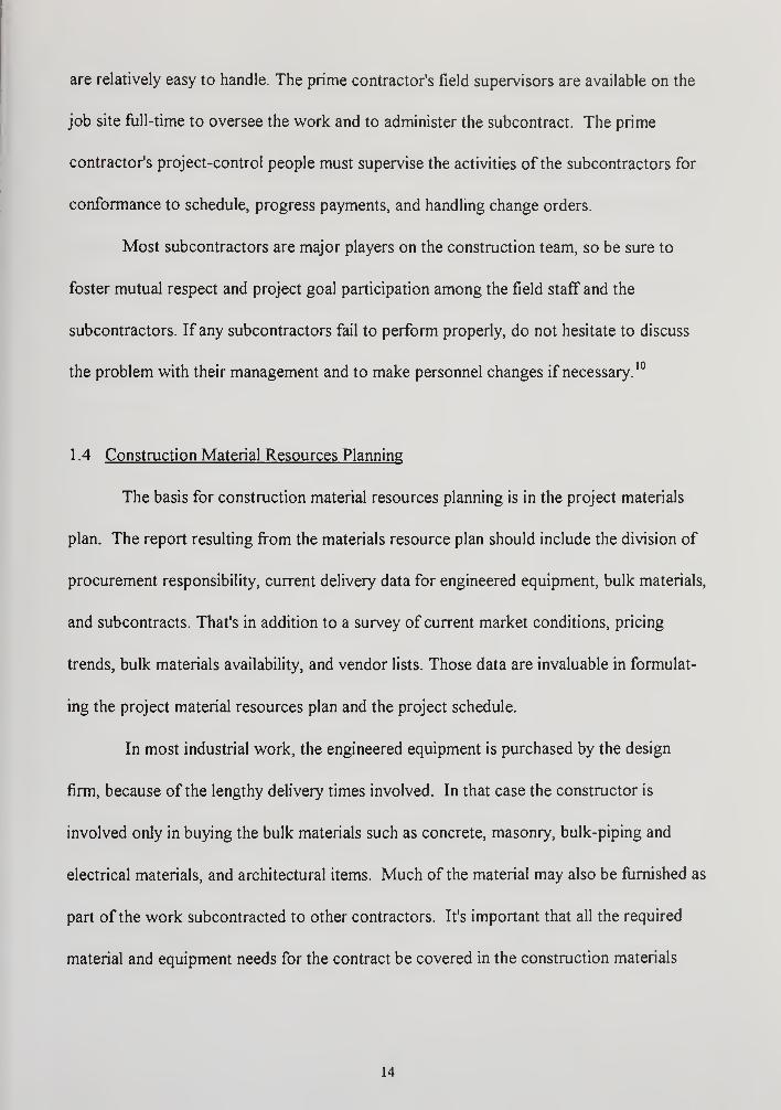
are relatively easy to handle. The prime contractor's field supervisors are available on the

job site full-time to oversee the work and to administer the subcontract. The prime

contractor's project-control people must supervise the activities of the subcontractors for

conformance to schedule, progress payments, and handling change orders.

Most subcontractors are major players on the construction team, so be sure to

foster mutual respect and project goal participation among the field staff and the

subcontractors. If any subcontractors fail to perform properiy, do not hesitate to discuss

the problem with their management and to make personnel changes if necessary.'°

1.4 Construction Material Resources Planning

The basis for construction material resources planning is in the project materials

plan. The report resulting from the materials resource plan should include the division of

procurement responsibility, current delivery data for engineered equipment, bulk materials,

and subcontracts. That's in addition to a survey of current market conditions, pricing

trends, bulk materials availability, and vendor lists. Those data are invaluable in formulat-

ing the project material resources plan and the project schedule.

In most industrial work, the engineered equipment is purchased by the design

firm, because of the lengthy delivery times involved. In that case the constructor is

involved only in buying the bulk materials such as concrete, masonry, bulk-piping and

electrical materials, and architectural items. Much of the material may also be furnished as

part of the work subcontracted to other contractors. It's important that all the required

material and equipment needs for the contract be covered in the construction materials

14

plan. It is vital to project success that the proper equipment and materials be available in

time to support the field construction schedule.''

Today's materials plan is usually a detailed document listing, by account code, the

quantities of the required materials and equipment, a description, their field-required date,

responsible supplier, and the like. A computerized spreadsheet or database is ideal for

handling the large quantity of information required to control the material on a medium- to

large-sized project. The daily update of the materials-tracking document makes

computerizing a must.

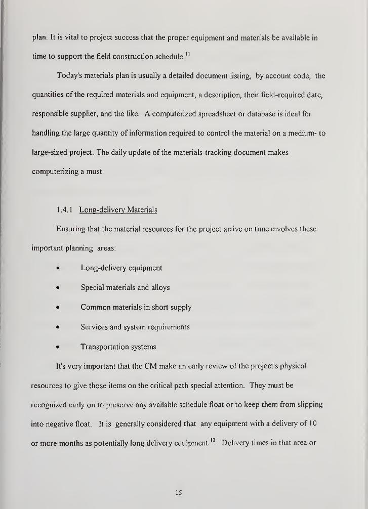
1.4.1 Long-delivery Materials

Ensuring that the material resources for the project arrive on time involves these

important planning areas:

Long-delivery equipment

Special materials and alloys

Common materials in short supply

Services and system requirements

Transportation systems

It's very important that the CM make an eariy review of the project's physical

resources to give those items on the critical path special attention. They must be

recognized early on to preserve any available schedule float or to keep them from slipping

into negative float. It is generally considered that any equipment with a delivery of 10

or more months as potentially long delivery equipment. '^ Delivery times in that area or

15

longer than 10 months usually place the equipment on the critical path. Examples of

long-delivery equipment for industrial projects include such items as sixty -ton air

conditioning units, centrifugal compressors, heavy-walled vessels, field-erected boilers, or

other complex engineered systems. We cannot assume that we do not have any of those

or similar items on your equipment list because almost every project has long-delivery

equipment. In most projects, the items with the longest delivery dates are the

long-delivery items.

Long-delivery items must be given top priority in the schedule, starting with the

first operations in the project design.

1.4.2 Special Materials and Alloys

It is a good idea to review all materials specified for the project that might not

normally be stocked because they are of a special nature. Some of these special materials

may also require special treatment such as casting, tube-bending, welding, and testing,

which tends to delay their delivery even further. Since most CMs are not strong in that

highly specialized area, it is best to have your technical staff or consultants thoroughly

investigate any potential delivery problem areas. Those long-delivery item reviews should

be made early enough that there is still time to deal with the problem. For example, the

design might call for a special aggregate in precast wall panels, special window systems, a

rare quarried and polished stone, or any one of many others that are likely to fall on the

critical path. Early planning for the delivery can get such an item off the critical path, and

that can pay a dividend of earlier job completion.^^

16

1.4.3 Common Materials in Short Supply

Common materials in short supply often include such ordinarily items as structural

steel, concrete, and reinforcing bars. For example, in a large high-rise building, the

structural steel will be high in tonnage. Eariy design and takeoff for placing mill orders

for the heavy steel is critical to maintaining the schedule. Each section of the structure

must be closely scheduled, if the steel is to be delivered at a time that suits the erection

sequence. A large dam project uses huge quantities of reinforcing steel, forms, earth fill,

and concrete over long periods of time. These relatively common materials must be

planned for and delivered on time if the schedule is to be met. These commonly used

materials sometimes tend to be overlooked on larger projects, so do not pass over them

lightly. That advice is especially valid if the project is being built in a remote location.

1.4.4. Services and Systems

Strictly speaking, project services and systems are not physical resources, but

they must be planned for at about the same time as the physical ones. Planning for them is

particularly critical on large projects.*'*

The project scheduling, accounting, cost-control, and administrative systems must

be decided on at this time, so that the necessary manual or computerized project-control

systems can be effectively implemented. If computers are to be used, the required

hardware, software, and communication resources must be planned and implemented.

Even such ordinary resources as the office service and the site facilities for construction

17

have to be planned early. Some items will fall on the critical path some will not, but the

critical items must be discovered early to allow for their resolution.

1.4.5 Transportation Svstems

Usually this category is involved only on large construction projects that may have

an international flavor, either in site location or in purchasing sources. Another special

case is construction projects that embody prefabricated modules built off site for erection

at remote locations. Any of that type of project will involve special loading,

transportation, and receiving facilities to handle unusually large pieces of equipment.

If the project involves a significant amount of foreign or imported equipment and

materials, the overall marshaling of shipments, import licenses, custom regulations,

dockside security, and invoicing should be developed by the project purchasing manager.

The traffic portion of the materials management plan must include all the legal and

quasi-legal factors involved in getting the goods to the construction site on time. The

CM must review the complete plan to assure that the field construction needs are being

fully supported. If the overall system does not function smoothly 100 percent of the time,

the field construction operations will be delayed.'^

1.5 Summary

This chapter wraps up the planning portion of the CM's activities. Effective CMs

must train themselves to plan all facets of the project, as well as their day-to-day work

activities.

18

i

We must remember, however, that a plan is only a proposed baseline for the

execution of a project. Any plan is subject to changes along the way. Although it is often

necessary to change our plans, it is not recommended making any radical changes to your

original plan. If our plans were well thought out, you should resist pressures to change

them.

19

CHAPTER TWORESOURCE HANDLING

2.1 Introduction

After we considered the timing or schedule of activities and the determination of

which activities control the project time, we have to consider questions about the

availability or most efficient usage of resources required to undertake the construction

operation. It is usually assumed that resources are available in doing the time calculations.

When activities are conducted simultaneously, it leads to simultaneous demands

for resources, producing peak resource demands at certain stages of the construction

project. Peak demands of resources, particularly over short periods of time, may be

undesirable. For example this implies, if workers are the resource, a "hire and fire"

situation. As we know, many resources in the construction industry tends to be

expensive and limited in number. Skilled labor is often difficult to obtain and costly to

fire. Resources not used effectively on site waste money.'^

Generally, it is more desirable to have approximately uniform resource

requirements. This means rescheduling certain activities such that resource requirements

are modified. The means for doing this rescheduling are to utilize the available float in the

network. A resource use graph or resource profile which is a plot of resource

requirements versus time, is found useful for regulating the resource demands. The ideal

situation would be to have a level resource use graph or a graph with a few changes in

level as possible.

20

Two distinct types of activities can be identified and can be termed intermittent

activities and continuous activities '^. With tiie former it is possible to break its operation

and restart at a later date. Resources associated with such activities are easier to handle in

the resource scheduling exercise than those associated with continuous activities.

Continuous activities, once started, must be carried on until completed. When beginning a

resource scheduling exercise, the engineer should be aware of the intermittent or

continuous nature of the project activities.

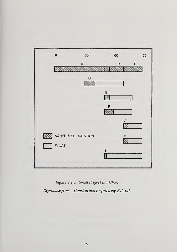
2.2 An Example

The bar chart in figure 2. 1 .a'^ and the activity information in Table 2. 1^' for a

small project can be used to plot the resource-use graph of figure 2. 1 .b ^°. The bar chart is

drawn for normal activity durations and for activities starting at their earliest date. The

resource, for example, could be workers. The resource usage graph represents the total

resource requirements for all activities over the project duration. The graph demostrates

the peak resource demand at certain stages of the construction project. Generally the

more uniform the resource demand the better. Once all the available float has been used

up, then the only recourse is to extend the total project time if fijrther resource levelling or

redistribution is required. In all cases, the starting point is the network calculation based

on normal times. These calculations are done assuming availability of resources.

21

30 60 90

Bm'ki!M!>'W.'iWki.'W'MWW'J ,lliiW,li-UMkWiil'J,Wi|'

..^^

SCHEDULED DURATION

FLOAT

H

Figure 2. 1.a Small Project Bar Chart

Reproducefrom : Construction Engineering Network

22

Resource

Level 20

10

1

E G

H

D

•

F

A 3 C

30 60

DAYS90

Figure 2. 1. b Resource Profile


Activity Dur EST LST EFT LFT TF Resource

Requirements

(/ Day)

A 50 50 50 7

B 20 50 50 70 70 4

C 20 70 70 90 90 4

D 10 30 60 40 70 30 6

E 5 50 75 55 80 25 4

F 10 50 70 60 80 20 6

G 3 70 87 73 90 17 4

H 4 70 86 74 90 16 7

1 2 50 88 52 90 38 6

Table 2.1 Activity information for example

Reproducefom : Construction Engineering Network

23

In place of plotting the resource requirements versus the time, the cummulative

resource requirements may be plotted. Figure 2.2 indicates the shape that such plots

take. Two plots are given: one corresponding to the activities starting as early as

possible, the other corresponding to the activities starting as late as possible^' . The

region between the two plots is where the final solution will and often lie. The straight

line, from project start to project completion, corresponds to uniform rersource usage.

800

600 -

Cumulative

(Resource)

Requirement

200• *

Earliest Start

Schedule

y^

.

// / Latest Start

Schedule^>y ^'

*

-^ V **

\Constant Slope Line

30 60 90

Days

Figure 2.2 Cumulative Resource Plot


24

For this example, letting workers be the resource, in a 90 day period the total

worker-days required are 702. This gives a uniform daily demand of workers of

702/90 = 8 workers.

2.3 Limited Resources

Where equipment, labor or materials (or capital) are restricted, the activities have

to be rescheduled to satisfy this form of constraint. Frequently this will imply scheduling

those activities that use such resources, in a sequential or serial fashion. And this might

create the situation where activities overrun their allowable float. This overrun situation

may also lead to an increased project completion time and the formation of a different

critical path.

If resource limitations are known at the start, for example, only one site crane is

available, then the original network plan for the project can include this constraint. In

particular this constraint determines which activities may be carried out concurrently and

which activities must wait for other activities to finish ( that is activity dependence).

In certain cases it may be possible to hire additional equipment to cover peak

requirements; in this case no rescheduling ofthe activities is called for.

As an example of a limited resource, assume that in the previous example only 10

units of the resource were available for the project. Clearly from figure 2.1.b, this

constraint is violated on a number of days. The means for resolving problems of limited

resources are similar to those for the problem in leveling and their discussion is

consequently carried over until leveling is treated.

One possible heuristic for allocating resources is as follows.

25

• For those activities whose earliest start times are the project start time,

assign the resource first to that activity with the least total float and then in

order increasing total float. This process may be terminated if all available

resources are used up or all activities have their requirements.

• Should all the resources be used up in the first step, the earliest times of

the remaining activities (yet to receive resource allocation) are increased.

Modify the subsequent parts of the network calculations accordingly.

• For those activities whose earliest start times correspond to when the

resources are next available, repeat first step.

2.4 Resource Leveling

There are major advantages involved in resource leveling, that is in reducing peak

demands for resources and creating a requirement for resources at other non-peak times.

In particular with regard to labour or plant, continuity in the workforce, in the recruitment

of labour and in the hiring or purchasing of plant are all desirable goals.

There are numerous approaches to the task of resource leveling. Some are

described below. There appears to be no one approach that has the consensus of engineers

using network programming. The case for a single resource is given first, followed by that

for multiple resources.

2.4.1 Single Resource

This approach first selects a target maximum for a resource (for example a

painting crew of 2 or 3 painters), and proceeds in time, that is from left to right in the

resource requirements versus time plot. Where this target level is exceeded, activities

contributing to this peak resource requirement are moved into their float time in such a

fashion that the peak requirement is removed or shifted. The activity duration may be

located anywhere within the interval bounded by that activity's EST and LFT.

26

There is no definitive rule as to which activities should be shifted. In one approach

those activities with the most float (preferably free float) are moved first in this

trial-and-error process, as these activities offer the most prospect for relocating the

activity to where total resource requirements are at or below the target level. Critical

activities remain untouched. Other approaches give first priority for being moved to

activities with the first-occurring latest start times and activities with the longest durations.

Small projects can often have their resources leveled by inspection.

On one pass through the resource plot, having relocated the starting times of

certain of the activities, should the target level still be exceeded, it may be necessary to

raise the target level and a second run made through the resource plot.

Example^^: For the example of Section 2.2, following priority rules of moving first

the activities with (i) the smallest total float or free float, (ii) the earliest LST or (iii) the

longest duration, the activities would be rescheduled, respectively, according to:

(i) Shift the starting dates of the activities in the following order: H, G, F, E, D, I

(ii) Shift the starting dates of the activities in the following order: D, F, E, H, G, I.

(iii) Shift the starting dates of the activities in the following order: F or D, E, H G,

and I. Some second priority rule would be necessary to distinguish between

moving F or D first.

The application of any one priority rule may not give the best leveled resource

solution and a combination of the priority rules coupled with inspection may be needed to

give the best solution. For example and by inspection, a reasonable start to the leveling

problem would shift activity D to a starting date of day 60, followed by moving the other

noncritical activities. Often a lot ofjuggling of the activity starting dates is required before

a suitable resource profile is obtained.

An alternative approach uses a resource plot based on activity start times

corresponding to their latest start times (LST). This provides a bound on the activity

27

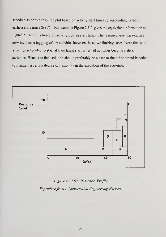
schedule as does a resource plot based on activity start times corresponding to their

earliest start times (EST). For example Figure 2.3^^ gives the equivalent information to

Figure 2. Lb but is based on activity LST as start times. The resource levelling exercise

now involves a juggling of the activities between these two limiting cases. Note that with

activities scheduled to start at their latest start times, all activities become critical

activities. Hence the final solution should preferably be closer to the other bound in order

to maintain a certain degree of flexiblility in the execution of the activities.

Resource

20

ll

Level

E G

10

D 1

F

H

A B C

30 60 90

DAYS

Figure 2.3 LST Resource Profile


28

2.4.2 Several Resources

Where the resource leveling exercise is to be carried out on several resources

simultaneously, again there are several approaches.

In one approach, the exercise is first carried out on the largest fluctuating resource

and so on down to the least fluctuating resource. This process may have to be repeated

several times, hopefully converging on a final solution.

In another approach, the resource which incurs the largest penalty, should it

fluctuate, is treated first. By implication the most costly resource is leveled first.

In another approach, first preference in resource leveling is given to equipment,

particularly the high cost items, and second preference is aimed at maintaining a

reasonably constant labour force. Whichever technique is used, there will generally be the

inevitable conflict involved in trying to satisfy all resource constraints simultaneously.

There is no real solution to this dilemma. There is no formal algorithm that covers the full

spectrum of problems that are encountered in the resource scheduling problem. Some

heuristic approaches do exist, however, that tackle parts of the resource scheduling

problem. The more successful are interactive, with the engineer doing part of the

computations.

The overall optimum resource scheduling solution may involve, as well as the

approaches above, time compression of certain activities particularly where the critical

activities are contributing to the difficulty of leveling resources. This topic is taken up in

the following chapter. Note here that optimum implies not only a consideration of the

direct costs associated with resources but also the indirect costs associated with the

29

project. Generally the idea of an optimum is a theoretical artifice and most solutions are

considered satisfactory if they are good or feasible. Where the number of activities is of a

manageable size, it is possible to use a computer graphics package to manipulate the

activities until a satisfactory resource levelled schedule is obtained.^'*

Resource leveling is treated further in Chapter 3 while resource constrained

scheduling is treated further in Chapter 4.

30

CHAPTER THREERESOURCE LEVELING

3.1 Introduction

Resource leveling is assigning resources to project activities in a manner that will

improve productivity and efficiency. In this chapter, we will deal with the labor, but the

same approach can be used for allocating other resources such as equipment and money.

Once the network diagram has been analyzed and all of the event times and activity

floats established, the scheduling of all projects activities may proceed. It is important to

realized, at this stage, that the individual activity durations used in the critical path

calculations imply a commitment to working each activity with sufficient resources to

ensure compatibility between the work volume involved in the activity and the

productivity and production rate achievable by these resources.

When developing the most up-to-date schedule, we are assuming that we had an

unlimited supply of all the resources needed for the tasks, but the real-world situation may

be very different. For example, the single crane we budgeted may be needed for two

construction tasks at the same time; or the carpentry crew may be required to work on

two or more different tasks at the same time; or the carpentry crew may be scheduled for

work on two or more overlapping tasks; or the painting crew will not be allowed to work

alongside the electricians in a confined space.

3.2 Leveling the Work Force

There are four reasons as to why we should level the work force^^

31

1. When the schedule demands more workers per day than are available or ifwe

have workers standing around without jobs, we have a problem.

2. When a new hire is trained, there is loss of productivity. So, ifwe can keep

the trained people and reduce the number of new hires, we should be better off.

3. As we know, every project suffers from start-up problems of some sort.

Superintendents and project managers are very busy trying to get every body working in

a productivity manner. Therefore, ifwe can start with a small crew and increase its size

gradually, we will eliminate some of the start-up problems.

4. Most projects suffer from congestion around project completion time because

of reduced work areas. Thus, ifwe can gradually reduce the crew size as we approach

project completion, we can improve productivity by reducing congestion.

3.3 The Leveling Procedure

The goal of any leveling procedure is to schedule all non-critical jobs so that the

resource pool is built up step by step to a peak and then allowed to drop off until the pool

is exhausted^^. This is done by:

• Scheduling all the critical jobs first.

• Starting the non-critical jobs whenever there is a drop in scheduled manpower

up to the point where the peak is reached.

• Starting the non-critical jobs whenever there is a drop so that no ups and

downs occur in the resource profile.

32

The significant factor in leveling is that the starting times for non-critical jobs only

are varied to produce a leveled schedule. The project duration is never extended.

3.4 Smoothing Resources

One goal of good management is to apply human resources in an effective and

efficient manner because on-again, off-again work periods are unsatisfactory to the

workers in a crew. We will use an example to illustrate such situations, define the

terminology, and explain the graphical aspects.

The basic Gantt Chart for a small project in Figure 3.1 shows when action is

FLOATL LABORER

4L

A12L

D

4L

F

4L

B

8L

C2L

E

2 4 6 8 10 12 14 16 18 20

Project Time in Days

Figure 3. J Daily Requirementfor Laborers: A Histogram.

being taken on each task and when specific resources are being used, in this case, laborers.

33

3.4.1 Resource Histograms

The number of workers needed by each task is written in each bar of the chart.

Using this manning data, we can construct a time-based graph showing the total number

ofworkers needed on each day of the project. This is called a resource histogram. A

separate histogram is needed for each resource, equipment utilization and labor

assignments. The histogram is based on every task starting at its Earliest Start Time and

the resource being used for the complete duration of the task. Figure 3.2 is the histogram

for laborers.

Number of

Laborers

20

18

C16

Crew Sizes

14

12

10

8

Target (12)

^^^^,^ /r\ o\' AVeidyc \v.u)

B D1

6 E

4

/\ F

2

2 4 6 8 10 12 14 16 18 20


Figure 3.2 Daily Requirementfor Laborers: A Histogram.

34

The total height of a box on the Gantt Chart indicates the total number of workers needed

from day to day, obtained by summing the number of workers from each task for that day.

It is useful to show the contribution from each task as a separate block on this histogram

because this will help later in planning where to relocate a particular task in the histogram.

3.4.2 Total Effort and Average Crew Sizes

A resource histogram provides another function as well: the area inside the graph

represents the total number of man-days required for the project. For example. Task "A"

needs four workers for 8 days; the effort required is 32 man-days (4 workers x 8 days).

Therefore, all the tasks in this small project require a total of 196 man-days over the 20

days of the project, an average of 9.8 workers per day. This gives us a target for

smoothing the workforce to less variable levels. Obviously we cannot have half-a-worker

so we must be content with a theoretical target of a constant crew often workers. After

making changes, we must ensure that the total effort is the same as before the changes,

196 man-days.

3.4.3 Smoothing the Daily Crew Allocations

In the example, we should strive to level each day's crew to the ten-person target,

but we may have to accept twelve as more realistic. At any rate, the 20 workers

scheduled for Days 8 through 12 are unacceptable. To resolve this overload, we need to

re-schedule several tasks to start later than their initially calculated Earliest Start Times.

We can accomplish this in two stages^^.

35

• "Freeze" the critical tasks (TF = 0) in their original time periods; then re-

schedule the others within their floats, starting with the task having the least

float. Note that tasks with TF = O have priority ONE. They are "fiôzen" in

time and are scheduled first (that is, in their original time period).

• If the crew size is still too large, re-schedule certain of the critical tasks to

minimize the increase in the duration of the project.

In our example, the priorities based on the Total Floats of the tasks are shown in

the table of figure 3.3. The technique works like this: Freeze tasks A, D, and F; then re-

schedule E, C, and B. With E left where it is, and C scheduled to start after D is finished,

then the original clash ofC and D is fixed but a new one is caused between C and E These

changes are displayed in Figure 3.3. Often, a "fi"ozen" task must be moved to a later time

slot to preserve the proper sequencing.

One way to satisfy the twelve-man requirement is to start E after F is finished,

causing E to become critical and extending the project by two day (see Figure 3.4). In this

case, E must be linked to both C and F to ensure that E cannot clash with either one ifC

or F slips with a longer duration. Alternatively, blindly placing C after F would solve the

overload but would lengthen the project by 4 days and cause an irregular crew size.

Projects normally start with a small crew, increase to a maximum near the middle,

and then fall off near the end. In this example, we could start Task "B" 4 days late (to

start the project "slower") with 4 workers for the first 2 days, followed by a fixed crew of

36

NumbLabor

20

18

16

14

12

10

8

6

4

2

erofers

Critical tasks are: A, D , and E (Total Float = 0)

jSecond

Target (12)

First

C/Third

DB

E

A F

2 4 6 8 10 12 14 16


18 20

Task Name A B C D

Total Float 12 8

Priority 14 3 1

E

2

2

F

1

Figure 3.3 Leveling the Histogram: Stage One

37

\

Number of

Laborers

Laborers Histogram:

Resolving Clash of

Task 'E'

14

12

10

8

6

4

2

D

C

B

A F

E

8 10 12 14 16 18 20 22

Project Days

I

Figure 5.4 Resolving the Second Clash

38

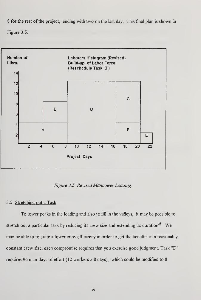
8 for the rest of the project, ending with two on the last day. This final plan is shown in

Figure 3.5.

Number of

Libra.

Laborers Histogram (Revised)

Build-up of Labor Force

(Reschedule Task 'B')

14

12

10

C8

B D6

4

/^ F

2 E

8 10 12 14 16 18 20 22

Project Days

Figure 3.5 RevisedManpower Loading.

3.5 Stretching out a Task

To lower peaks in the loading and also to fill in the valleys, it may be possible to

stretch out a particular task by reducing its crew size and extending its duration . We

may be able to tolerate a lower crew efficiency in order to get the benefits of a reasonably

constant crew size; each compromise requires that you exercise good judgment. Task "D"

requires 96 man-days of effort (12 workers x 8 days), which could be modified to 8

39

workers for 12 days or 6 workers for 16 days, each of which results in 96 man-days of

effort. This stretching technique is useful if an extended project duration is acceptable.

The small project we have been using as an example has been stretched; it is shown in

Figure 3.6.

Number of

Laborers

10

8

6

4

2

B

D CE

A F

8 10 12 14 16 18 20 22 24 26 28

Project Days

Figure 3. 6 Stretching Out a Task

3.6 The Technique: Steps for Resource Leveling

The following are the steps for resource leveling29.

• Schedule the task having the EARLIEST Late Start Time (this gives priority to

the earliest critical task—for critical tasks, LST = EST) and then reschedule the

task having the next earliest LST, and so on.

• When several tasks have the same LST, give priority to the one having the

smallest Total Float.

40

• Schedule each task as early as possible without violating any of the prece-

dence requirements for the project. When a critical task slips, any task

following it must also start later. Refer continually to the network or

Precedence Matrix to maintain the order of construction. You can ensure that

construction sequencing is not violated by adding links to the network based

on the sequencing dictated by your smoothing objectives.

• Ensure that the total amount of each resource scheduled does not exceed the

prescribed limit; it measures the total effort expended by a crew.

3.6.1 Smoothing More Than One Resource at a Time

This introduction to "smoothing" has focused on smoothing only one resource:

laborers. Realistically, there will be more than one type of manpower and equipment that

clash among themselves and must be smoothed^". Realistic multiple clashes are

practically impossible to smooth to their ideal levels because re-scheduling one could

cause a clash in another. Compromises must be made. The manager must decide which

resource should be "smoother" than the others. If smooth manpower loading is preferable

to the smooth use of machinery, then this criterion will guide the re-scheduling of tasks.

3.6.2 Checking Your Work: Bookkeeping Checks Reveal Errors

As we re-schedule a task, its resource bar will be moved along the row and

therefore the sums in the bottom row will change; the sum in the last column will not be

changed. We must remember to keep track of the effort for each resource each day and

41

record the totals in the lower rows at the bottom of the page. When we have finished, we

can check our accuracy by summing the totals of the last column and comparing it with

the sum of values in the bottom row. They should be the same. An example is shown in

Figure 3.7, which is based on the small example project described in Figure 3.1.

FLOAT

4L

L LABORERS

A 32

96

"16

~8

32

4

12L

D

4L

F

4L

B

8L

C

2L

E

8 8 8 8 4 4 4 4 20 20 20 20 12 12 12 12 6 6 4 4 1 9 6

2 4 6 8 10 12 14 16 18 20


Figure 3. 7 Checking the Worksheet

And just as important, the terms in the last column must be the same as they were before

you re-scheduled. If not, then you made mistakes. These values in the last row and the

last column represent the effort expended for each task on any given day; the total in the

lower right corner is the total effort required for the project. This is so because the

42

fundamental assumption of this method is to reschedule without changing the total

resources of any task.

3.7 Summary

There is much in this chapter about leveling resources by modifying the schedule of

individual construction tasks. We found that the critical tasks could be "frozen" in their

original schedule and that the remaining tasks might be re-scheduled within their individual

floats. It might become necessary for critical tasks to be re-scheduled, with a resulting

extension of the project.

We needed to be careful to ensure that the original precedence requirements were

not violated after some tasks were re-scheduled. It is always more challenging to try to

level several resources at once rather than only one.

43

I

CHAPTER FOURCONSTRAINED RESOURCE SCHEDULING

4.1 Introduction

The previous chapter examined the process of leveling resources in order to get

maximum utilization from the resources. No mention was made of restrictions

(constraints) on the availability of resources. However resources are often limited. This

tends to require the shifting of activities forward in time until resources are available,

leading to a consequent extension of the total project duration.

There are two fundamental approaches to constrained allocation problems:

heuristics and optimization models. Heuristic approaches employ rules that have been

found to work reasonably well in similar situations. They seek better solutions.

Optimization approaches seek the best solutions but are far more limited in their ability to

handle complex situations and large problems.

4.2 Heuristic Methods^^

Heuristic approaches to constrained resource scheduling problems are use for a

number of reasons. To begin with, they are the only feasible methods of attacking the

large, nonlinear, complex problems that tend to occur in the real world of project

management. Second, while the schedules heuristics generate may not be optimal, they

are usually quite good . Commercially available computer programs handle large problems

and have had considerable use in industry. The heuristic approach attempts to keep the

project duration at a minimum while satisfying any resource restrictions, maximizing

resource utilization and maintaining resource requirements reasonably level. As discussed

44

in chapter three, the float of non-critical activities provides the means for shifting activities

so as to shift the resource requirements. However, priority rules must be established.

The approach provides a satisfactory solution in reasonable computational time. It

also permits the tackling of networks larger than that permitted by any exact mathematical

formulation of the problem. It is seen that by allowing activities to be split, extended or

compressed, a scheduling better in resource utilization and shorter in duration may be

obtained. However, it is recognized that many construction activities do not lend

themselves to such modifications.

Most heuristic solution methods start with the CPM schedule and analyze

resource usage period by period, resource by resource. In a period when the available

supply of a resource has exceeded, the heuristic method examines the tasks in that period

and allocates the most scarce resource to them sequentially, according to some priority

rule. Some of the more common priority rules are these:

• Select resources with the shortest task first. This rule will maximize the

number oftasks that can be completed by a system during some time period.

• Select resources first that require a higher demand on scarce resources.

• Select resources with the minimum slack first. This heuristic orders activities

by the amount of slack, least slack going first.

• Select most critical followers tasks. The ones with the greatest number of

critical followers go first.

There are many such priority rules employed in scheduling heuristics. Several

researchers have conducted tests of the more commonly used schedule priority rules .

45

Although their findings vary somewhat because of slightly different assumptions, the

minimum slack rule was found to be best and almost never caused poor performance. It

usually resulted in the minimum amount of project schedule suspension .

One of two events will result as the scheduling heuristic operates . First, the

routine runs out of activities before it runs out of the resources, or it runs out of

resources before all activities have been scheduled. While it is theoretically possible for

the supply of resources to be precisely equal to the demand for such resources, even the

most careful planning rarely produces such a neat result. If the former occurs, the excess

resources are left idle, assigned elsewhere in the organization as needed during the current

period, or applied to future tasks required by the project. If one or more resources are

exhausted, however, activities requiring those resources are slowed or delayed until the

next period when resources can be reallocated.

If the minimum slack rule is used, resources would be used in critical or nearly

critical activities, and delaying those with greater slack. Delay of an activity uses some of

its slack, so the activity will have a better chance of receiving resources in the next

allocation. Repeated delays move the activity higher and higher on the priority list. We

consider later what to do in the potentially catastrophic event that we run out of resources

before all critical activities have been scheduled.

4.2.1 An Example

Consider, for example, the following project scheduling problem.

Given the network and resource demand shown in Figure 4.1, find the best schedule using

46

a constant crew size. Each day of delay beyond 15 days incurs a penalty of $2,000.

Workers cost $200 per day, and machines cost $100 per day. Workers are

interchangeable, as are machines. Task completion times vary directly with the number of

workers, and partial work days are acceptable. The critical time for the project is 15 days,

given the resource usage shown in Figure 4.1.

Reproducefrom: Project Management

Figure 4. 1 Networkfor Resource Load Simulation^\

Note: The numbers on the arcs represent, respectively, worker-days, machine-day

Figure 4.1 lists the total man-days and machines per day normally required by each activity

(below the activity arc). Because activity times are proportional to worker input, the

critical path is b-c-e-i, and this path uses 149 man-days.

47

The fact that completion times vary with the number of workers means that ac-

tivity a could be completed in 6 days with ten workers or in 10 days with six workers.

Applying some logic and trying to avoid the penalty, which is far in excess of the cost of

additional resources, we can add up the total man-days required on all activities, obtaining

319. Dividing this by the 15 days needed to complete the project results in a requirement

of slightly more than twenty-one workers. Ifwe rounded off, it would be twenty-two.

How should they be allocated to the activities? Figure 4.2 shows one way, arbitrarily

determined. Workers are shown above the "days" axis and machines below. We have 22

workers at $200 per day for 15 days ($66,000) and 128.5 machine days at $100 per day

($12,850). The total cost of this particular solution is $45,850. We could remove some

manpower from those tasks not on the critical path. If a given activity has slack, we could

trade some or all of the slack for a resource saving. Take activity j, for example. It has 1.2

days of slack. Our basic assumption is that 10 workers can do activity j in 5.5 days. Ifwe

use the slack, j can take up to 6.7 days without delaying the project. Using this slack, we

can reduce the manpower required from 10 to 8.2, saving 1.8 workers for use on a critical

task. If the manpower loading on task / is increased by 1.8 workers, the task time is cut to

3.1 days. It is reduced to 33/34.8 or 98.4 percent of its original value. The path b-c-d-j

is now critical. Activity slack in other activities can be used in a similar way. If this is not

true, the relationship must be known activity by activity, and the amounts of

workers/machines that can be shifted subject to the constraints implied by machine

flexibility.

48

i

woRKERS

MACHI

NES

24

20

16

12

8

4

2

6

8

10

12

b (12,4)c

(12,2)

a (10 workers,

6 days)

e (10,4.5)

d (3,3.7)

f(6,3)

h

(9,

i.ir

g(3,5)

j (14,3.9)

i (8.4)

12 18DAYS

Cost

Workers $66,000

Machines 12.850

Total $78,850

Reproducefrom : Project Management

Figure 4.2 Load chartfor a Simulation Problem^''

The purpose of these reassignments is not to decrease labor cost in project. This is

fixed by the base technology implied by the worker/mach usage data. The reassignments

do, however, shorten the project duration; make the resources available for other work

49

sooner than expected. If the trade ofFs are among resources, for instance, trading more

manpower for fewer machines or more machines for less material input, the problem is

handled the same way.

On small networks with simple interrelationships among the resources, it is not

difficult to perform these resource trade-offs by hand. But for networks of a realistic size,

a computer is clearly required. If the problem is programmed for computer solution, many

different solutions and their associated costs can be calculated. But, as with heuristics,

simulation does not guarantee an optimal, or even feasible, solution. It can only test those

solutions fed into it.

Another heuristic procedure for leveling resource loads is based on the concept of

minimizing the sum of the squares of the resource requirements in each period. That is,

the smooth use of a resource over a set of periods will give a smaller sum of squares than

the erratic use of the resource that averages out the same amount as the smooth use. This

approach, called Burgess's method, was applied by Woodworth and Willie^^ to a multi-

project situation involving a number of resources. The method was applied to each

resource sequential starting with the most critical resource first.

4.2.2 Heuristics Techniques'^

Since there are many problems with the analytical formulation of realistic

problems, major efforts in attacking the resource-constrained multi-project scheduling

problem have centered on heuristics. We mention earlier on some of the common general

50

criteria used for scheduling heuristics. The most commonly applied rules were discussed

in Section 4.2.

Resource Scheduling Method: This give precedence to that activity with the

minimum value of <i where

w • • ^^ increase in project duration resulting when activityy follows activity /,

y

-Max' J)

v/hQveEFT. = early finish time of activity /

LSTj = latest start time of activity^

Minimum Late Finish Time: This rule assigns priorities to activities on the basis of

activity finish times as determined by CPM. The earliest late finishers are scheduled first.

Greatest Resource Demand: This method assigns priorities on the basis of total

resource requirements, with higher priorities given for greater demands on resources.

Project or task priority is calculated as:

mPriority = a '— y r..

where u • — duration of activity

y

T' '"^ per period requirement of resource / by activityy

U

51

i

171 number of resource types

Resource requirements must be stated in common terms, usually dollars. This

heuristic is based on an attempt to give priority to potential resource bottleneck activities.

Greatest Resource Utilization: This rule gives priority to that combination of

activities that results in maximum resource utilization or minimum idle resource during

each scheduling period. This rule was found to be approximately as effective as the

minimum slack rule for multiple project scheduling, where criterion used was project

slippage.

Heuristic procedures for resource-constrained multi-project scheduling represent

the only practical means for finding workable solutions to the large, complex multi-project

problem normally found in the real world.

4.3 Optimizing Methods

The methods to find an optimal solution to the constrained resource scheduling

problem fall into two categories: mathematical programming (linear programming for the

most part) and enumeration. In the 1960s, the power ofLP improved fi"om being able to

handle three resources and fifteen activities to four resources and fifty-five activities. But

even with this capacity, LP is usually not feasible for reasonably large projects where there

may be a dozen resources and thousands of activities.^^ In the late sixties and early

seventies, limited enumeration techniques were applied to the constrained resource

problem with more success.

52

4.3.1 Mathematical Programming

Mathematical programming can be used to obtain optimal solutions to certain

types of multi-project scheduling problems. These procedures determine when an activity

should be scheduled, given resource constraints. It is important to remember that each of

the techniques can be applied to the activities in a single project, or to the projects, in a

partially or wholly interdependent set of projects. Most models are based on integer

programming that formulates the problem using 0-1 variables to indicate whether or not

an activity is scheduled in specific periods.

In spite of its ability to generate optimal solutions, mathematical programming has

some serious drawbacks when used for resource allocation and multi-project scheduling.

As noted earlier, except for the case of small problems, this approach has proved to be

extremely difficult and computationally expensive.

4.4. Multi-project Scheduling and Resource Allocation

Scheduling and allocating resources to multiple projects is much more complicated

than for the single-project case. The most common approach is to treat the several

projects as if they were each elements of a single large project. Another way of attacking

the problem is to consider all projects as completely independent. These two approaches

lead to different scheduling and allocation outcomes. For either approach, the conceptual

basis for scheduling and allocating resources is essentially the same.

When there are several projects, each has its own set of activities, due dates, and

resource requirements. In addition, the penalties for not meeting time, cost, and

53

performance goals for the several projects may differ. Usually, the multi-project problem

involves determining how to allocate resources to, and set a completion time for, a new

project that is added to an existing set of ongoing projects. This requires the development

of an efficient, dynamic multi-project scheduling system.

To describe such a system properly, standards are needed by which to measure

scheduling effectiveness. Three important parameters affected by project scheduling are^^:

(1) schedule slippage, (2) resource utilization, and (3) in-process inventory. The

organization must select the criterion most appropriate for its situation.

Schedule slippage, often considered the most important of the criteria, occurs

when the project is past its due date or delivery date. Slippage can result in paying penalty

costs; and this will reduce profits. Further, slippage may caused other projects to slip.

A second measure of effectiveness is resource utilization. This is of particular

concern to industrial firms because of the high cost of making resources available. A

resource allocation system that smoothes out the peaks and valleys of resource usage is

ideal, but it is extremely difficult to attain while maintaining scheduled performance

because all the projects in a multi-project organization are competing for the same scarce

resources^^. In particular, it is expensive to change the size of the human resource pool on

which the firm draws. While it is relatively easy to measure the costs of excess resource

usage required by less than optimal scheduling in an industrial firm, the costs of uncoor-

dinated multi-project scheduling can be high in service-producing firms.

The third standard of effectiveness is the amount of in-process inventory. It

concerns the amount of work waiting to be processed because there is a shortage of some

54

resource(s). Most industrial organizations have a large investment process inventory,

which may indicate a lack of efficiency and often represents a major source of expense for

the firm. The remedy involves a trade-off between the cost of in-process inventory and the

cost of the resources, usually capital equipment, needed to reduce the in-process inventory

levels. All these criteria cannot be optimized at the same time. As usual, trade-offs are

involved. A firm must decide which criterion is most applicable in any given situation, and

then use that criterion to evaluate its various scheduling and resource allocation options.

As noted earlier, experiments by Fendley revealed that the minimum slack-first rule

if the best overall priority rule, generally resulting in minimum project slippage, minimum

resource idle time, and minimum system occupancy time for the cases he studied^". But the

most commonly used priority rule is 'first come, first served" which has little to be said

for it except that it fits the client's idea of what is "fair". In any case, individual firms may

find a different rule more effective in their particular circumstances and should evaluate

alternative rules by their own performance measures and system objectives.

4.5 Summary

In this chapter, we have shown the two basic approaches to addressing the

constrained resources allocation problem.

Heuristic methods which are realistic approaches that may identify feasible

solutions to the problem. They essentially use simple priority rules, such as shortest task

first, to determine which task should receive resources and which task must wait.

Optimizing methods, such as linear programming, find the best allocation of resources to

55

tasks but are limited in the size of problems they can efficiently solve. Mathematical

programming models for multi-project scheduling aim either to minimize total throughput

for all projects, minimize the completion time for all projects, or minimize the total

lateness for all projects. These models are limited to small problems.

56

CHAPTER FIVECOMPUTER APPLICATIONS IN RESOURCE LEVELING

5.1 Introduction

The method of resource allocation discussed in the previous two chapters involved

simple arithmetic and data manipulation. As one can see, however, that to perform

complete resource allocation manually for even an average sized project would be

impractical and it would be almost impossible for a large project. Although there are

many software applications that do resource leveling such as Primavera, Microsoft

Project Manager, Suretrack, etc., this chapter will be entirely dedicated to Primavera

project planner since it is the most common.

5.2 Allocating Resources in Primavera version 11 for Windows

This section will give a brief introduction as to how to assign resources , designate

driving versus non-driving resources, set resource limits, and check for overloads using

on-screen histograms. It will also explain how to refine a resource plan.

5.2.1 Defining a Resource Plan

We define a resource plan by building a list of resources needed to accomplish the

project goals and assigning these resources to activities. When assigning resources, we

need to decide whether the resource drives the duration of the activity and to check

whether the schedule requires more resources than are available by producing resource

profiles.'*^

57

5.2.1.1 Assigning Resources

Here, we need to use the "Resources" form to assign resources to

activities. We display tiie "Resources form" from "the Activity form"; and size and

position them so that we can review activity details as we assign resources.

For each resource we need to enter the units per day or budget quantity. If we

enter units per day, P3 calculates the quantity to complete by multiplying the

amount you enter by the number of days required to complete the activity"*^:

Quantity to Complete = Remaining Duration x Units Per Day

At the start of a project, P3 sets the budgeted and forecasted quantities equal to

this quantity to complete. Ifwe enter the total budgeted amount for the resource,

P3 calculates its rate of use (units per day) as follows"^:

Units Per Day = Budgeted Quantity x Remaining Duration

We can also express resource units as person-days per day, quantities of

material to be installed per day (such as linear feet), or any other type of unit. We

can assign as many resources per activity as we need . We can simply accomplish

this by clicking + on the edit bar in the "Resources" form to add

assignments. When we finish, we choose the "OK" button in the Activity form

58

to save our edits. The "OK" and "Cancel" buttons change to "Previous" and

"Next" buttons so we can quickly select the previous or next activity in the table

and continue to assign resources.

5.2.1.2 Driving Resources

The duration of an activity sometimes depends on the number of resources

assigned to it. In general, the more resources assigned, the less time is required to

complete the activity. For example, ifa task the requires 1 60 mandays for

testing the software, and ifwe assign 8 person per day, P3 will schedule 20 days

to complete the activity. Ifwe were to double the resource amount reduces the

task duration to 10 days.

In P3, we can define a resource as "driving," which means that the number

of resources assigned to an activity determines its duration. To specify a resource

as driving for a specific activity, we check the "Driving" box for that resource.

Then, enter the total effort required (budget quantity) and the number of units per

time period for the resource. P3 calculates a resource duration, which is used as

the activity duration. Ifwe assign more than one driving resource to an activity,

the resource that requires the most time to complete determines the original and

remaining durations for the activity.

To assign resources we do the following'*'*:

1 . Choose "Display", "Activity Form" and click the "Res" (resources)

button to open the blank Resources form. Or select an activity and

59

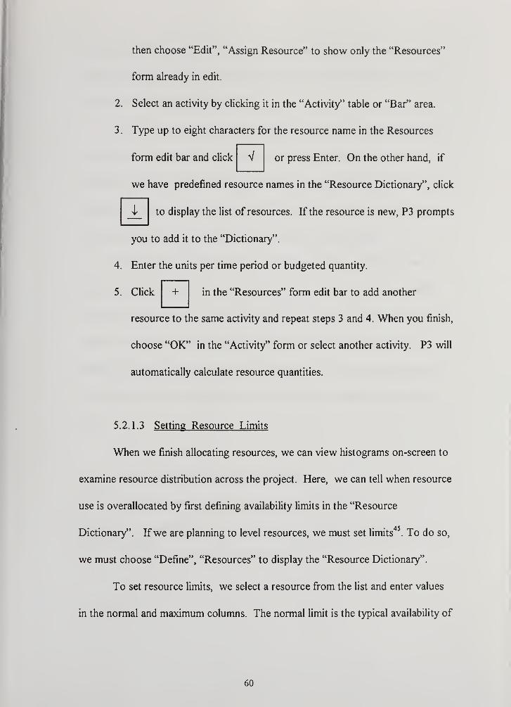
then choose "Edit", "Assign Resource" to show only the "Resources"

form already in edit.

2. Select an activity by clicking it in the "Activity" table or "Bar" area.

3. Type up to eight characters for the resource name in the Resources

form edit bar and click V or press Enter. On the other hand, if

we have predefined resource names in the "Resource Dictionary", click

to display the list of resources. If the resource is new, P3 promptsi

you to add it to the "Dictionary".

4. Enter the units per time period or budgeted quantity.

5. Click + in the "Resources" form edit bar to add another

resource to the same activity and repeat steps 3 and 4. When you finish,

choose "OK" in the "Activity" form or select another activity. P3 will

automatically calculate resource quantities.

5.2.1.3 Setting Resource Limits

When we finish allocating resources, we can view histograms on-screen to

examine resource distribution across the project. Here, we can tell when resource

use is overallocated by first defining availability limits in the "Resource

Dictionary". Ifwe are planning to level resources, we must set limits'*^ To do so,

we must choose "Define", "Resources" to display the "Resource Dictionary".

To set resource limits, we select a resource from the list and enter values

in the normal and maximum columns. The normal limit is the typical availability of

60

the resource while the maximum is the highest amount of the resource that is

available at one time. For example, the carpenter is usually available for 8 hours

but he can work up to 10 hours per day.

We can also use P3's on-screen graphics to determine whether resources

are sufficient to complete the scheduled work. If a profile shows that some

activities need more resources than are available, use P3's leveling feature to

redistribute resources across the schedule. We can also expand or compress the

timescale of a resource by adjusting the timescale on the Bar chart.

When we click the "Emphasize" overload with colors checkbox, the bar

color changes as resource use exceeds the limits. Green bars indicate use vidthin

availability, yellow bars mean that resource use exceeds the normal limit but is still

within the maximum, and red bars signal usage above the maximum limits of

availability. When choosing draw limits, P3 draws a yellow horizontal line across

the profile at the normal availability limit, and a red line to define the maximum

limit.

5.2.1.4 How to Create a Resource Profile

To create a resource profile, we must do the following'*^:

1. Choose "Display", "Resource Profile". P3 displays a profile for the first

resource in the "Resource Dictionary".

61

2. Click i and choose a resource from the list. Scroll to the

bottom of the list and choose "Total" to display a profile for all

resources defined for the project.

3. Choose the "Display" button to change options. For example, display

units or costs; choose a different time interval; choose whether to show

total (combined), peak (highest), or average (total/number of time units

in interval) use; and choose whether you want to show bars, curves, or

both.

4. Use the "Select" button to choose multiple stacked resources or

grouped resources. To stack resources, use different group numbers

and colors for each line of resource selection. To group resource usage

in one bar, assign the same group number and color to each line of

resource selection.

To close the resource profile, choose "Display", "Resource Profile" again.

5.2.1.5 Resource Tables

Resource tables show as listing of resource distribution over time. It

summarizes the total number of resources per day, week, month, quarter, or year.

We can specify whether to display peak, total, or average-use values.

To create a resource table , we must do the following :

1 . Choose "Display", "Resource Table".

62

2. Click i and choose a resource from the list. P3 creates and

displays a table for all resources, beginning with the resource you

selected.

3. Click the "Display" button to modify options.

4. To choose specific resources, click the "Select" button. Assign a

unique row number to each line of resource or cost-account selection

One can group resources in the same row by assigning them the same

row number. In this case, use the "Group Name" column to define a

title for the resource group.

5.2.2 Refining the Resource Plan

We refine the resource plan by reallocating resources or defining specific lags and

durations to reflect the actual start and end dates for resource use. If resource use is

nonlinear, we can use a resource curve to accurately define resource distribution across

the activity. If resources are still overloaded, we can level them.

5.2.2.1 Adjusting the Resource Distribution

When we assign resources in P3, their use starts when an associated

activity starts and continues until the activity completes. However, we can use

resource lags and durations to control the times resource use begins and ends. A

lag is a delay between the start of the activity and the start of the resource use";

for example, a resource may not be needed until a few days after an activity begins.

63

I

\

i

'

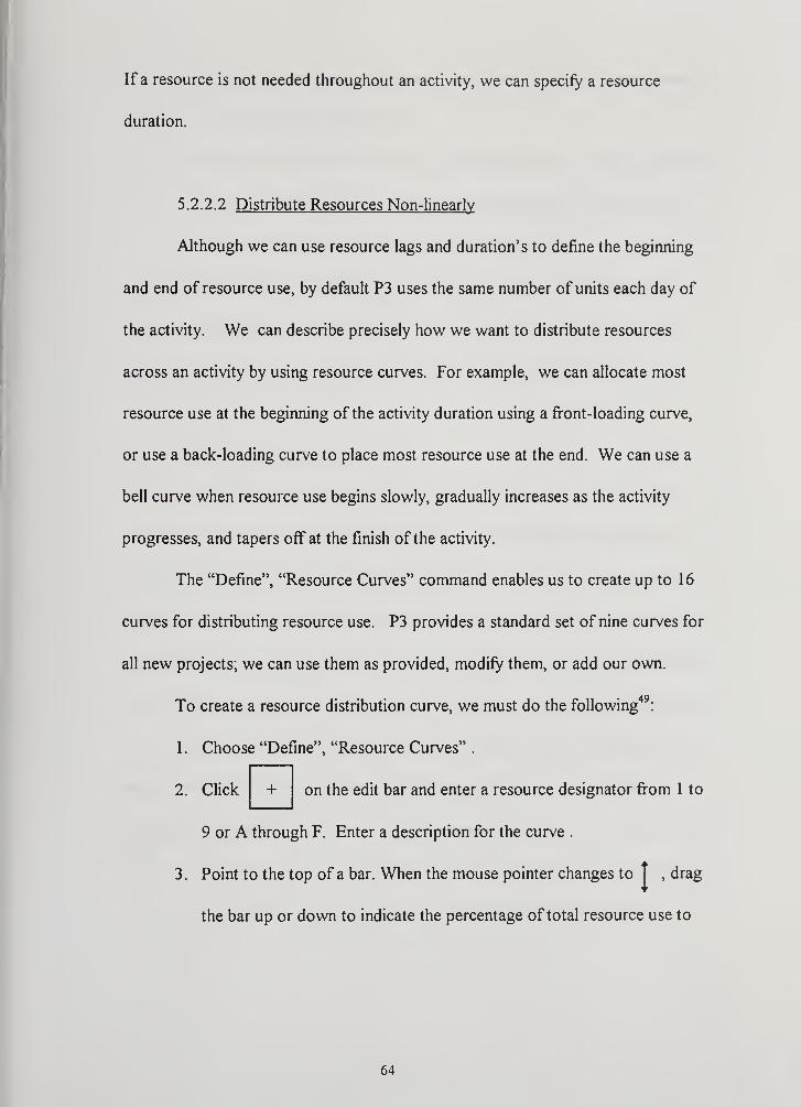
If a resource is not needed throughout an activity, we can specify a resource

duration.

5.2.2.2 Distribute Resources Non-linearlv

Although we can use resource lags and duration's to define the beginning

and end of resource use, by default P3 uses the same number of units each day of

the activity. We can describe precisely how we want to distribute resources

across an activity by using resource curves. For example, we can allocate most

resource use at the beginning of the activity duration using a fi"ont-loading curve,

or use a back-loading curve to place most resource use at the end. We can use a

bell curve when resource use begins slowly, gradually increases as the activity

progresses, and tapers off at the finish of the activity.

The "Define", "Resource Curves" command enables us to create up to 16

curves for distributing resource use. P3 provides a standard set of nine curves for

all new projects; we can use them as provided, modify them, or add our own.

To create a resource distribution curve, we must do the following :

1 . Choose "Define", "Resource Curves" .

on the edit bar and enter a resource designator fi-om 1 to2. Click +

9 or A through F. Enter a description for the curve .

3. Point to the top of a bar. When the mouse pointer changes to T , drag

the bar up or down to indicate the percentage of total resource use to

64

I

allocate for that percent of activity duration. We can also enter specific

values along the bottom row.

4. Choose the "Prorate" button to recalculate the values so they total 100

percent. Choose "OK". Use the "Restore" button to return the curve

to its original values before the changes are applied.

Check resource availability once curves are assigned; we may need to

change resource distributions to avoid overloads. We can use these curves in

conjunction with resource leveling to produce an optimal resource plan.

5.2.2.3 Level Resources

After using resource lags and curves to refine the resource plan, and if

profiles show that some activities still need more resources than are available, we

can use P3's leveling feature to redistribute critical resources across the schedule.

Resource leveling compares the allocation of resources to availability and delays

certain activities to remain within these limits. Resource leveling does not change

activity durations or resource requirements; it can, however, delay schedule dates.

During leveling, P3 reschedules activities whose combined resource needs

exceed the availability limits defined in the "Resource Dictionary". Before an

activity can be rescheduled, however, all its predecessors must be completed, and

all the necessary resources for the activity must be available for the entire duration

of the activity. P3 delays the activity until both requirements are satisfied.

65

P3 provides several options for resource leveling. We can level the entire

project or, ifwe are only concerned with resource requirements for the next 2

weeks, for example, we can save processing time by leveling only as far as the

cutoff date you specify.

We can also specify whether P3 levels forward or backward. P3 normally

levels activities according to their early schedule dates, starting with the first

activity v^th no predecessors and continuing to the last activity in the network;

this is called forward leveling. P3 can also perform backward leveling, in which

activities are leveled using their late schedule dates. In a backward-leveled

schedule we can see the latest possible dates for activities without exceeding

resource availability. When we backward level, P3 moves activities forward in

time, instead of delaying them.

P3 always produces an analysis report that shows the results of leveling

resources. When we level a project, we can produce additional reports, such as a

tabular schedule, to examine the effects of leveling on the entire schedule.

An additional option enables us to smooth resources based on time or

resource constraints. Resource smoothing uses positive float to minimize sharp

changes in resource use. During non-time-constrained smoothing, P3 makes

several attempts to schedule an activity within the maximum availability limit of the

resource, thereby reducing the possibility of delays. When time is more important

than resource availability, time-constrained resource smoothing automatically

doubles the maximum resource limit in an attempt to schedule the activity without

66

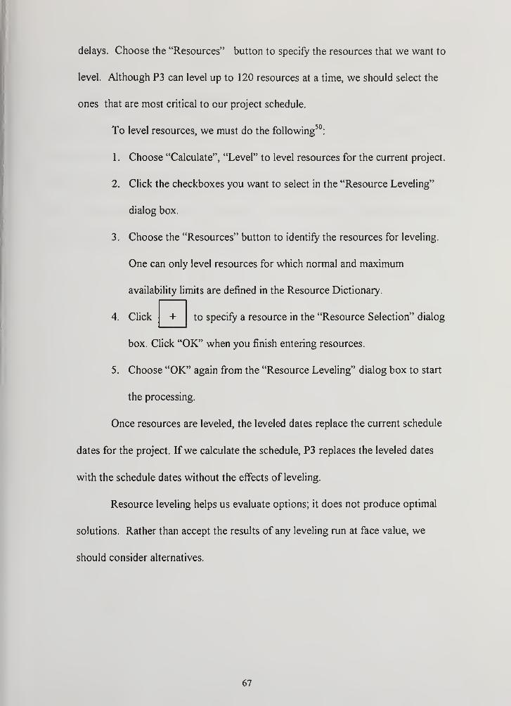
delays. Choose the "Resources" button to specify the resources that we want to

level. Although P3 can level up to 120 resources at a time, we should select the

ones that are most critical to our project schedule.

To level resources, we must do the foliowing^°:

1. Choose "Calculate", "Level" to level resources for the current project.

2. Click the checkboxes you want to select in the "Resource Leveling"

dialog box.

3. Choose the "Resources" button to identify the resources for leveling.

One can only level resources for which normal and maximum

availability limits are defined in the Resource Dictionary.

4. Click + to specify a resource in the "Resource Selection" dialog

box. Click "OK" when you finish entering resources.

5. Choose "OK" again from the "Resource Leveling" dialog box to start

the processing.

Once resources are leveled, the leveled dates replace the current schedule

dates for the project. Ifwe calculate the schedule, P3 replaces the leveled dates

with the schedule dates without the effects of leveling.

Resource leveling helps us evaluate options; it does not produce optimal

solutions. Rather than accept the results of any leveling run at face value, we

should consider alternatives.

67

I

i

i

5.3 Summary

Although there are many software applications as well as computer programs that

can help us with resource leveling, Primavera project planner is the one software

application that most project managers use today. This application has managed to

reallocate resources or juggle the schedule to resolve conflict between activities that use

the same resources. It also helps us to level our resource plan and examine the resource

use to determine whether the plan contains hard to manage peaks and valleys.

6S

CONCLUSION

The construction industry today is facing more and more challenges than ever

before. This includes increased complexity of projects, more costly projecând stricter

rules and regulations under which to operate. Without the proper resource allocation,

one will pay the price for late job completions and cost overruns.

Resource allocation as described in this report must start with a good solid plan .

It cannot be accomplish without defining four essential elements which are materials,

people, equipment, and time. Therefore, planning is very essential since many projectjzan

suffer unavoidable delays fiôm inadequate resource planning. In the planning phase, we

must identify the required resources needed to complete the project.

After we have identified the resources needed to complete the project, we must be

able to allocate them in order to undertake the construction operation. When applying

resource leveling, we assumed that we have an unlimited supply of resources required for

the tasks, but we must remember that the real world situation may be different. The goal

of resource leveling is to assign resources to project activities in a manner that will

improve productivity and efficiency.

As mentioned before, resources are often limited and this tends to shift the

activities forward in time until resources become available. In this report we have

presented two ways to approach constrained allocation problems. These were the

heuristics and optimization models. The former one jdentifies feasible solutions to the

problem using simple priority rules , such as shortest task first, to determine which task

should receive resources and which task must wait. The latter solution finds the best

69

i

allocation of resources to tasks but limits the size of problems that can be efficiently

solved.

Although there are several software computer applications such as Microsoft

project planner, suretrack, and other programs that dp resource leveling, the last chapter

of this report c'over^ resource leveling using Primavera project planner since is it the

software application that most project managers use nowadays. .

During the last two decades, the construction industry has progressed in this trend

of improving resource allocation iiot merely out of interest but as a means of survival in a

more competitive world. However, it is apparent that in the future^resource planning and

resource allocation will still present considerable challenge^nd source dt frustration to

researchers in/niathematics and operations research.

70

REFERENCES

1. Clough, Richard H. and Sears, Glenn A. , Construction Project Management . John

Wiley & Sons, Inc., New York, 1991, pp. 157-158.

2. Westney, Richard E., Managing the Engineering and Construction of Small Projects .

Marcel Decker, Inc., New York, 1985, p. 67.

3. Ritz, George J., Total Construction Project Management . McGrraw-Hill, Inc., NewYork, 1993, p. 182

4. Ritz. op. cit. . p. 183

5. Ritz. op. cit. . p. 184

6. Ibid.

7. Ritz. op. cit. . p. 186

8. Ritz. op. cit. .pp. 185-188

9. Ibid .

10. Ritz. op. cit. . p. 191

11. Ritz. op. cit. .p. 192

12. Ritz, op. cit., p. 193-194

13. Ritz. op. cit. .p. 195

14. Ritz. op. cit. . p. 196

15. Ritz. op. cit. .p. 197

16. Carmichael, D. G. , Construction Engineering Networks . John Wiley & Sons, Inc.,

1989, p. 65

17. Ibid .

18. Carmichael, op. cit. , p. 66


71

i

I

I

I

I





24. Carmichael, op. cit., p. 71

25. Stevens, James D., Techniques for Construction Network Scheduling . McGraw-Hill,

Inc., 1990, pp. 123-124

26. Ahuja, H. N. , Construction Performance Control bv Networks . John Wiley & Sons,

Inc. , 1976, pp. 241-242

27. Naylor, Henry, Construction Project Management . Delmar Publishers. 1995, pp. 145

28. Naylor, op. cit. . p. 148



3 1

.

Meredith, JackR. and Samuel J. Mantel Jr., Project Management . John Wiley &Sons, Inc., Second Edition, 1989, p. 340

32. Meredith, op. cit. . p. 341

33. Meredith, op. cit ., p. 342



36. Meredith, op. cit . , pp. 348-349

37. Ahuja, op. cit. . pp.221-225

38. Ibid.

39. Ibid.

40. Fenley, L. G. , "Towards the development of a complete Multi-project Scheduling

System", Journal of Industrial Engineering . Oct 1978

72

I

I

41. Microsoft, Primavera Project Planner . Primavera Systems, Inc., 1993, p. 120

42. Microsoft, op. cit. , p. 121

43. Ibid

44. Microsoft, op. c







.,pl22

.,p. 123

,pl27

,pl29

,p. 130

,pl33

,pp. 136-137

73

I

BIBLIOGRAPHY

Adrian, James J. , CM: The Construction Management Process , Reston Publishing

Company, Inc. , 1981, pp. 169-206

Adrian, James J. , Construction Productivity Improvement . Elsevier Science Publishing

Co., Inc., 1987, pp. 211-257

Adrian, James J. , Microcomputers in the Construction Industry . Prentice Hall Company,

1985, pp. 178-228

Ahuja, H. N., Construction Performance Control by Networks . John Wiley & Sons,

Inc., 1976, pp. 201-298

Carmichael, D. G. , Construction Engineering Networks . John Wiley & Sons, Inc.,

1989, pp. 65-97

Clough, Richard H. and Glenn A. Sears, Construction Project Management . John

Wiley & Sons, Inc., Third Edition, 1991, pp. 157-179

Frankel, Ernst G., Project Management in Engineering Services and Development .

Butterworth & Co. (Publishers) Ltd., 1990, pp. 36-39

Hendrickson, Chris and Tung Au, Project Management for Construction . Prentice Hall,

1989, pp. 297-335

Halpin, Daniel W. and Ronald W. Woodhead, Construction Management . John Wiley &Sons, Inc., 1980, pp. 313-335

Meredith, Jack R. and Samuel J. Mantel Jr., Project Management. John Wiley & Sons,

Inc., Second Edition, 1989, pp. 327-354

Microsoft, Primavera Project Planner . Primavera Systems, Inc., 1993, pp. 119-138

Naylor, Henry, Construction Project Management . Delmar Publishers, 1995, pp. 121-

160

Nunally, S. W. , Construction Methods and Management . Regents/Prentice Hall, 1993,

pp. 361-385

O'Brien, James, CPM in Construction Management . McGrawHill, Inc., Second

Edition, 1971, pp. 190-217

74

Popescu, Calin M., Project Planning. Scheduling, and control in Construction . John

Wiley & Sons, Inc., 1995, pp. 51-73

Ritz, George J., Total Construction Project Management . McGraw-Hill, Inc., 1994,

pp. 181-199

Stevens, James D., Techniques for Construction Network Scheduling . McGraw-Hill,

Inc., 1990, pp. 123-141

Westney, Richard E., Managing the engineering and Construction of Small Projects .

Marcel Decker, Inc., 1985, pp. 197-218

Willis, Edward, Scheduling Construction Projects . John Wiley & Sons, Inc., 1986, pp.

321-337.

75

I

DUD! = y KN'OX LIBRARYNAVAL POSTGRADUATE SCHOOLMONTEREY CA 93943-5101

GAYLORD S

Documents

Resource planning and resource allocation in the