Sediment interstitial waters and diagenesis

Interstitial waters are aqueous solutions that occupy the pore spaces between particles in rocks and sedi-ments. In some nearshore deposits groundwater seepages can occur, and around the ridge -crest areas circulating hydrothermal solutions (i.e. modifi ed sea-water) can enter the sediment column. For most marine sediments, however, the interstitial fl uids originated as seawater trapped from the overlying water column. The interstitial -water–sediment complex is a site of intense chemical, physical and biological reactions, which can lead both to the formation of new and altered mineral phases and to changes in the composition of waters themselves. These changes may be grouped together under the term diagenesis,which has been defi ned by Berner (1980) as ‘thesum total of processes that bring about changes in a sediment or sedimentary rock subsequent to its deposition in water ’. Many of the important diage-netic changes that affect marine sediments take place during early diagenesis, which occurs during the burial of the deposits. The highest rates of bio-logical activity occur in the top tens of cm of the sediments but biological activity is now known to continue to depths in excess of 1 km (Roussel et al., 2008).

14.1 Early diagenesis: the diageneticsequence and redox environments

14.1.1 Introduction

Many of the chemical changes that take place during early diagenesis are redox -mediated, that is, they depend on the redox (chemical reduction/oxidation reactions) environment in the sediment –interstitial-water–seawater system. In turn, this redox environ-

14

ment is largely controlled by the degree to which organic carbon is preserved, or undergoes decompo-sition, in the sediment complex. Most of the ocean water column is oxic, and hence the degradation in the water column occurs mainly with oxygen as the oxidizing agent. However, within the ocean sedi-ments oxygen can become depleted and alternative oxidizing agents become important. Oxidation of organic carbon can use alternative electron acceptor and is now chemically defi ned as the loss of electrons (See Worksheet 14.1).

14.1.2 The diagenetic sequence

Diagenetic processes in sediments are driven by redox reactions that are mediated by the decomposi-tion of organic carbon, and some of the basic con-cepts involved in sedimentary redox processes are described in Worksheet 14.1.

It is now generally recognized that there is a dia-genetic sequence of catabolic processes in sediments, the nature of which depends on the particular oxidiz-ing agent that ‘burns’ the organic matter. As sedimen-tary organic matter is metabolized it donates electrons to various oxidized components in the interstitial -water–sediment complex, and when oxygen is present it is the preferred electron acceptor. During the diagenetic sequence, however, the terminal electron-accepting species alter as the oxidants are consumed in order of decreasing energy production per mole of organic carbon oxidized. Thus, as oxygen is exhausted, microbial communities switch to a suc-cession of alternative terminal electron acceptors in order of decreasing thermodynamic advantage (see e.g. Froelich et al., 1979; Galoway and Bender, 1982;Wilson et al., 1985). Using the schemes outlined by,

290

Marine Geochemistry, Third Edition. Roy Chester and Tim Jickells. © 2012 by Roy Chester and Tim Jickells. Published 2012 by Blackwell Publishing Ltd.

Sediment interstitial waters and diagenesis 291

Worksheet 14.1: Redox r eactions in s ediments

Aqueous solutions do not contain free protons and free electrons. However, according to Stumm and Morgan (1996) it is possible to defi ne the relative proton and electron activities in these solutions. Acid – base processes involve the transfer of protons, and pH, which can be written

pH H= − +log10 a (WS14.1.1)

which measures the relative tendency of a solution to accept or transfer protons. The activity of a hypothetical hydrogen ion is high at low pH and low at high pH, and pH is a master variable in acid – base equilibria.

In a similar manner, it is also possible to defi ne a convenient parameter to describe redox intensity. Redox reactions involve the transfer of electrons, and p ε , which can be written

p aε = − −log10 e (WS14.1.2)

which measures the relative tendency of a solution to accept or transfer electrons. A high p ε indi-cates a relatively high tendency for oxidation, and p ε is a master variable in redox equilibria.

An oxidation – reduction reaction is termed a redox reaction, and can be written as two half - reactions in which a reduction is accompanied by an oxidation in terms of a redox couple. To illustrate this, Drever (1982) used the reduction of Fe 3 + by organic matter, represented by (C). Thus:

4 2 4 432

22Fe C H O Fe CO H+ + ++ ( ) + → + + . (WS14.1.3)

In this equation neither molecular oxygen nor electrons are shown explicitly. The equation can be broken down into two half - reactions, one involving only Fe and the other only C. Thus:

4 4 43 2Fe e Fe+ − ++ → (WS14.1.4)

in which Fe 3 + undergoes reduction to Fe 2 + , and

C H O CO H e( ) + → + ++ −2 4 42 2 (WS14.1.5)

in which the organic matter undergoes oxidative destruction to yield CO 2 . It must be remem-bered, however, that these half reactions do not represent complete chemical reactions because aqueous solutions do not contain free electrons.

The half - reaction concept can be related to measurements in electrochemical half - cells, and allows another parameter to be introduced into redox chemistry. This parameter is E h , in which the electron activity is expressed in volts, the h subscript indicating that the E h value is expressed relative to the standard hydrogen electrode, which is used as a zero reference. The relative activ-ity of electrons in a solution can therefore be expressed in units of electron activity ( p ε ), which is a dimensionless quantity, or in volts ( E h ), and the relation between p ε and E h is given by:

pFRT

Eε =2 3.

h (WS14.1.6)

where F is Faraday ’ s constant, R is the gas constant and T is the absolute temperature; at 25 ° C E h = 0.059 p ε . It is possible to measure E h using electrodes, analogous to the measurement of pH. However, electrode - measured E h values in oxidizing natural waters are diffi cult to relate to a specifi c redox pair, and both Stumm and Morgan (1996) and Drever (1982) have pointed out that it is important to distinguish between electrode - measured E h and E h calculated from the activities of a redox pair.

continued on p. 292

292 Chapter 14

In the present text the general concept of redox conditions will be used, in which positive E h (redox potential) values indicate oxidizing conditions and negative values indicate reducing conditions; that is, half - reactions of high E h are oxidizing, and those of low E h are reducing. Thus, a half - reaction with a lower E h will undergo oxidation when combined with a half - reaction of higher E h . This reaction combination can be used to describe redox - mediated diage-netic reactions in sediments. E h can be converted to energy units (e.g. Fig. WS14.1.1 ) and hence describes the thermodynamic, but not necessarily the kinetic, tendency for a reaction to proceed.

E h conditions in sediments are controlled mainly by the decomposition of photosynthetically produced organic matter by non - photosynthetic bacteria, and are constrained by the rate of supply of the organic matter (primary production), the rate at which it accumulates (sedimen-tation rate) and the rate of supply of oxidizing agents. The breakdown of organic matter is carried out almost exclusively by bacteria. However, this bacterial decomposition of organic matter is driven by a sequence of reactions that switch to a successive series of oxidants, or electron acceptors, which represent lower p ε levels and hence lower energy yields. During the reaction sequence, in which the organic matter is decomposed by micro - organisms, the organ-isms acquire energy for their metabolic requirements and communities able to carry out the highest energy yielding reactions will always dominate.

Only relatively abundant elements with oxidation states that can change under conditions found within the environment will play an important role in sedimentary diagenetic redox reactions. Hence, only a relatively few elements (C, N, O, S, Fe and Mn) are predominant participants in aquatic redox processes, although the redox state of other trace components may be altered. The overall relationships that involve these elements in the microbially medi-ated redox sequence have been summarized diagrammatically by Stumm and Morgan (1996) ; their scheme is reproduced in Fig. WS14.1.1 in which the energy yields associated with the various half reaction processes in the diagenetic sequence are given in the form of reaction combinations that are initiated at various E h and p ε values. These are illustrated in Fig. WS14.1.1 and Table WS14.1.1 . For example, the fi rst stage in the sequence involves the oxida-tion of organic matter by dissolved oxygen (A + L), with successive reactions following the decreased p ε and E h levels. The full ‘ diagenetic sequence ’ , and the sedimentary environments associated with the various stages in the sequence, are discussed in detail in the text. Examples

continued

Table WS14.1.1 Environmentally Important Reduction and Oxidation Reactions (Stumm and Morgan, 1996 ) at pH7, p ε values are for reactions proceeding left to right, but all are theoretically reversible. Letters refer to Fig WS14.1.1. Note M, N, O and P are the reverse of reactions G, E, D and C respectively. The energy of organic matter (simplifi ed here to CH 2 O) oxidation depends on the products for example, F and L. e represents an electron transferred in the reaction.

p ε

A + 13.75 B + 12.65 C + 8.9 D + 6.15 E − 0.8 F − 3.01 G − 3.75 H − 4.13 J − 4.68 L − 8.2

FeOOH HCO H e FeCO H Os aq aq s( ) ( ) ( ) ( )+ + + → +− +3 3 22 2

1 2 1 2 3 2 1 22 3 3 2/ Mn IV O / HCO / H e / Mn II CO Hs aq aq s( ) ( )( ) ( ) ( ) ( )+ + + → +− + OO

1 2 1 22 3/ CH O H e / CH OHaq+ + →+( )

1 8 9 8 1 8 1 242

2/ SO / H e / HS / H Oaq aq− + −+ + → +( ) ( )

1 4 212 2/ O H e H Og aq( ) ( )+ + →+

1 5 6 5 1 10 3 53 2 2/ NO / H e / N / H Oaq aq g( ) ( ) ( )− ++ + → +

1 8 5 4 1 8 3 83 4 2/ NO / H e / NH / H Oaq aq aq( ) ( ) ( )− + ++ + → +

1 8 1 8 1 42 4 2/ CO H e / CH / H Og aq g( ) ( ) ( )+ + → ++

1 6 4 3 1 32 4/ N / H e / NHaq aq+ + →+ +( ) ( )

1 4 1 4 1 42 2 2/ CH O / H O / CO H eaq g aq( ) ( ) ( )+ → + ++

Sediment interstitial waters and diagenesis 293

of the diagenetic succession are given in the box, in Fig. WS14.1.1 , where the overall energy yield of the combined reactions are given. From this it can be seen, for example, that there is a tendency for the more energy - yielding reactions to take precedence over those that are less energy - yielding. Thus, the sequence begins with aerobic respiration (A + L), followed by deni-trifi cation (B + L), and so on.

Fig. WS14.1.1 The microbially mediated diagenetic sequence in sediments (from Stumm and Morgan, 1996 ). The relative energy yield of the various redox half reactions are presented in term of decreasing energy yield (as Eh, p ε , and Δ G). Arrows point in the direction of the spontaneous reaction with the starting point representing the energy for that particular half reaction. The half reactions A to P are listed in the box.

Fe (II)Fe (III) oxide

0–5 +5–10

O2 – Formation

+10 +15 +20 pε

R

0–5 +5 p02+51+01+01– ε

0–10 +0.5 +1.0 EH Volt

N2Q

Oxidat of Mn (II)P

NO3–

NH4+O NO3

–

Oxidat of Fe (II)N

SulfideM SO42–

Oxidat org MatL

N2 Formation K

N2 JNH4+

N42– Fermentation H

SO42– Reduction G

Reduct org Mat F

E

NO3 Reduction D

M (II)Mn (IV) oxide C

Denitrification B

O2 – Reduction A

Aerobic RespirationDenitrificationNitrate ReductionFermentationSulfate ReductionMetane Fermentation

A + LB + LD + LF + LG + LH + L

– 29.9– 28.4– 19.6

–6.4–5.9–5.6

Examples

Combination ΔG°pH = 7Kcal/equiv

N – Fixation J + L – 4.8

Sulfide OxidationNitrification

A + MA + O

– 23.8– 10.3

Fereous OxidationMn (II) Oxidation

A + NA + P

– 21.0– 7.2

5 10

Kcal/equivalent

20

Reductions

Oxidations

294 Chapter 14

ferred electron acceptor, a reaction that can be represented as follows:

5 472

276 520 5 8862 106 3 16 3 4 3

2 2 3 4 2

CH O NH H PO HNO

N CO H PO H

( ) ( ) ( ) +→ + + + OO

(14.2a)

This process is termed denitrifi cation . The green-house gas N 2 O can be produced a by - product of this reaction as discussed in Section 9.1 In the reaction given above it is assumed that all organic nitrogen released is in the form of ammonia, which is then oxidized to molecular nitrogen by the reaction:

5 3 4 93 3 2 2NH HNO N H O+ → + (14.2b)

However, this is not the only possible pathway, and Froelich et al. (1979) have pointed out that the fate of the nitrogen has important consequences in diagenesis with respect to the sequence in which the secondary oxidants are used. These authors sug-gested that if all the nitrogen goes to N 2 then the use of nitrate as a secondary oxidant overlaps with that of MnO 2 , but that if the nitrogen is released as ammonia and is not oxidized to N 2 then MnO 2 should be reduced before nitrate. This emphasises that the complexities of the ocean often confound simplistic chemical representation.

The use of the other secondary oxidants can be illustrated by reactions of the type described by Froelich et al. (1979) for the use of Mn(IV), Fe(III) and sulfate as alternative electron acceptors for the degradation of organic matter with Redfi eld stoichiometry. 2 Manganese oxides

CH O NH H PO MnO H

Mn CO N H

2 106 3 16 3 4 2

22 2

236 472

236 106 8

( ) ( ) ( ) + +

→ + + +

+

+33 4 2336PO H O+

(14.3)

3 Iron oxides

CH O NH H PO Fe O H

Fe CO NH

2 106 3 16 3 4 2 3

22

212 848

424 106 16

( ) ( ) ( ) + +

→ + +

+

+33 3 4 2530+ +H PO H

(14.4)

4 Sulfate

CH O NH H PO SO

CO NH S H PO

2 106 3 16 3 4 4

2 32

3 4

55

106 16 55

106

( ) ( ) ( ) +

→ + + ++

−

HH O2

(14.5)

among others, Froelich et al. (1979) and Berner (1980) , the general diagenetic sequence in marine sediments can be outlined in the following general way.

Aerobic m etabolism. Aerobic organisms can use dissolved oxygen from the overlying or interstitial waters to ‘ burn ’ organic matter. The organic matter that undergoes early diagenesis can be considered to have the Redfi eld composition of (CH 2 O) 106 (NH 3 ) 16 (H 3 PO 4 ) (see Section 9.2 ). The oxidation of organic matter by aerobic organisms therefore can be repre-sented by a general equation such as that proposed by Galoway and Bender (1982) :

5 690

530 80 5 6102 106 3 16 3 4 2

2 3 3 4 2

CH O HN H PO O

CO HNO H PO H O

( ) ( ) ( ) +→ + + + ..

(14.1)

The CO 2 released during this reaction can lead to carbonate dissolution, and the ammonia can be oxi-dized to nitrate, a process termed nitrifi cation . Under oxic conditions most of the remains of dead animals and plankton are apparently destroyed at this stage in the diagenetic sequence. For example, according to Bender and Heggie (1984) , > 90% of the organic carbon that reaches the deep - sea fl oor is oxidized by O 2 . Oxygen therefore may be regarded as the primary oxidant involved in the destruction of organic matter, and in a closed system reaction (reaction 14.1 ) (oxic diagenesis) will continue until suffi cient oxygen has been consumed to drive the redox potential low enough to favour the next most effi cient oxidant. Thus, as dissolved oxygen becomes depleted, organic matter decomposition can continue using oxygen from secondary oxidant sources (suboxic diagenesis).

Anaerobic m etabolism. Anaerobic metabolism takes over when the content of dissolved oxygen falls to very low levels, or becomes entirely exhausted, and a series of secondary oxidants are utilized depending on their energy yields (see Worksheet 14.1 where a simpler representation of organic composition is used). These secondary oxidants include nitrate, MnO 2 , Fe 2 O 3 or FeOOH and sulfate. 1 Nitrate . According to Berner (1980) , when the dissolved oxygen levels fall to ∼ 5% of their concen-tration in aerated waters nitrate becomes the pre-

Sediment interstitial waters and diagenesis 295

3 Non - sulfi dic post - oxic environments . These envi-ronments, which contain no measurable dissolved sulfi des, are common in many deep - sea sediments, and are perhaps more often referred to in the litera-ture as suboxic environments. The condition neces-sary to set up this type of sedimentary environment is a supply of organic carbon suffi cient that diagen-esis can proceed beyond the oxic stage. Under these conditions, nitrate, manganese oxides and iron oxides are used as secondary oxidants, but the sequence does not reach the stage at which sulfate is utilized for this purpose. In suboxic sediments, there-fore, there is a relatively large, but still limited, supply of metabolizable organic matter, and the dia-genetic sequence has proceeded to the reactions in Equations 14.2 – 14.4 given previously. 4 Sulfi dic environments . These result when the dia-genetic sequence has reached the stage at which the bacterial reduction of dissolved sulfate takes place with the production of H 2 S and HS − . If a suffi cient supply of metabolizable organic matter is available, sulfate reduction can be a common feature in marine sediments as a result of the relatively high concentra-tion of sulfate in both seawater and marine sediment interstitial waters. In practice, however, constraints on the supply and preservation of organic matter mean that sulfate reduction is largely restricted to nearshore sediments where organic carbon supply is relatively high. In sulfi dic environments the diage-netic sequence has now proceeded to Equation 14.5 . The production of sulfi de is particularly important because it is toxic to many larger organisms and also because it will react with many metals to form very insoluble sulfi des. These include: iron sulfi des, such as the polysulfi de pyrite (FeS 2 ) and its diamorph mar-casite (FeS 2 ); the metastable iron sulfi des mackenaw-ite and greigite; glauconite; chamosite; manganese sulfi de (MnS). For a detailed description of these minerals the reader is referred to Calvert (1976) . 5 Non - sulfi dic methanic environments . In some sed-iments that contain a relatively large amount of metabolizable organic matter the diagenetic reac-tions can pass through the stage at which oxygen, nitrate, manganese oxides, iron oxides and sulfate are sequentially utilized. Continued decomposition of organic matter results in the formation of dis-solved methane, for example by reactions in Equa-tions 14.6a and 14.6b with methane released as bubbles from the sediment.

5 Following sulfate reduction, biogenic methane can be formed by two possible reaction pathways, which may be generalized as:

CH COOH CH CO3 4 2→ + (14.6a)

or

CO H CH H O2 2 4 28 2+ → + (14.6b)

Thus, diagenesis proceeds in a general sequence in which the oxidants are utilized in the order: oxygen > nitrate > manganese oxides > iron oxides > sulfate. In this diagenetic sequence it is assumed that in marine sediments O 2 , NO3

−, MnO 2 , Fe 2 O 3 (or FeOOH) and SO4

2− are the only electron acceptors, and that organic matter (represented by the Redfi eld composition) is the only electron donor. Further-more, it is assumed that the oxidants are limiting, that is, each reaction proceeds to completion before the next one starts. However, the diagenetic pro-cesses are not always sequential; for example, although it is usually thought that sulfate reduction precedes methane formation, Oremland and Taylor (1978) have suggested that the two processes can occur simultaneously, that is, they are not mutually exclusive.

14.1.3 Diagenetic and redox environments

As diagenesis proceeds a number of end - member sedimentary environments are set up, which Berner (1981) was able to relate to a diagenetic zone sequence. 1 Oxic environments are those in which the intersti-tial waters of the sediments contain measurable dis-solved oxygen, and diagenesis occurs via aerobic metabolism. Under these conditions in deep ocean sediments often little organic matter is preserved in the sediments, and in terms of the reactions given above the diagenetic sequence has proceeded only to the reaction in Equation 14.1 in oxic environments. Thus, the oxygen supply exceeds the degradable organic matter on, or in, the sediments. 2 Anoxic environments are those in which the sedi-ment interstitial waters contain no measurable dis-solved oxygen, that is, diagenesis here has to proceed via the secondary oxidants through anaerobic metabolism. The anoxic environments were subdi-vided into a number of types.

296 Chapter 14

there was no indication that the sediments had entered the sulfate reduction zone.

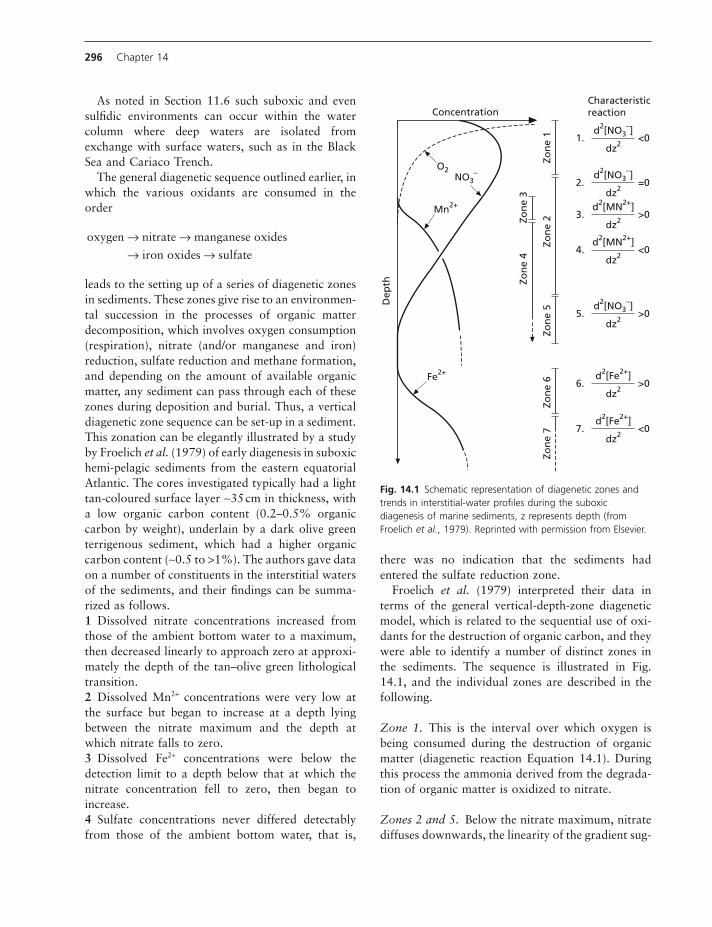
Froelich et al. (1979) interpreted their data in terms of the general vertical - depth - zone diagenetic model, which is related to the sequential use of oxi-dants for the destruction of organic carbon, and they were able to identify a number of distinct zones in the sediments. The sequence is illustrated in Fig. 14.1 , and the individual zones are described in the following.

Zone 1. This is the interval over which oxygen is being consumed during the destruction of organic matter (diagenetic reaction Equation 14.1 ). During this process the ammonia derived from the degrada-tion of organic matter is oxidized to nitrate.

Zones 2 and 5. Below the nitrate maximum, nitrate diffuses downwards, the linearity of the gradient sug-

As noted in Section 11.6 such suboxic and even sulfi dic environments can occur within the water column where deep waters are isolated from exchange with surface waters, such as in the Black Sea and Cariaco Trench.

The general diagenetic sequence outlined earlier, in which the various oxidants are consumed in the order

oxygen nitrate manganese oxides

iron oxides sulfate

→ →→ →

leads to the setting up of a series of diagenetic zones in sediments. These zones give rise to an environmen-tal succession in the processes of organic matter decomposition, which involves oxygen consumption (respiration), nitrate (and/or manganese and iron) reduction, sulfate reduction and methane formation, and depending on the amount of available organic matter, any sediment can pass through each of these zones during deposition and burial. Thus, a vertical diagenetic zone sequence can be set - up in a sediment. This zonation can be elegantly illustrated by a study by Froelich et al. (1979) of early diagenesis in suboxic hemi - pelagic sediments from the eastern equatorial Atlantic. The cores investigated typically had a light tan - coloured surface layer ∼ 35 cm in thickness, with a low organic carbon content (0.2 – 0.5% organic carbon by weight), underlain by a dark olive green terrigenous sediment, which had a higher organic carbon content ( ∼ 0.5 to > 1%). The authors gave data on a number of constituents in the interstitial waters of the sediments, and their fi ndings can be summa-rized as follows. 1 Dissolved nitrate concentrations increased from those of the ambient bottom water to a maximum, then decreased linearly to approach zero at approxi-mately the depth of the tan – olive green lithological transition. 2 Dissolved Mn 2 + concentrations were very low at the surface but began to increase at a depth lying between the nitrate maximum and the depth at which nitrate falls to zero. 3 Dissolved Fe 2 + concentrations were below the detection limit to a depth below that at which the nitrate concentration fell to zero, then began to increase. 4 Sulfate concentrations never differed detectably from those of the ambient bottom water, that is,

Fig. 14.1 Schematic representation of diagenetic zones and trends in interstitial - water profi les during the suboxic diagenesis of marine sediments, z represents depth (from Froelich et al. , 1979 ). Reprinted with permission from Elsevier.

Characteristicreaction

Dep

th

Mn2+

Concentration

NO3–

O2

d2[NO3–]

<01.dz2

Zon

e 1

Zon

e 3

Zon

e 4

d2[NO3–]

=02.dz2

d2[MN2+]>03.

dz2

d2[MN2+]<04.

dz2

d2[NO3–]

>05.dz2

d2[Fe2+]>06.

dz2

d2[Fe2+]<07.

dz2

Zon

e 2

Zon

e 5

Zon

e 6

Zon

e 7

Fe2+

Sediment interstitial waters and diagenesis 297

dissolved oxygen in the interstitial waters the sedi-ments can become reducing, and ultimately anoxic, at depth as the diagenetic sequence proceeds. The depth at which the oxic –anoxic change occurs depends largely on a combination of the magnitude of the down -column carbon fl ux, by which the carbon is supplied, and the sediment accumulation rate, by which it is buried since For example, accord-ing to Muller and Mangini (1980) a bulk sedimenta-tion rate of ≤1–4cm 10 3 yr−1 is necessary for the deposition of an oxygenated sedimentary column. Thus, the thickness of the surface sediment oxic layer will tend to increase from nearshore to pelagic regions as the accumulation rate decreases. The organic carbon content of sediments ranges from <0.25 to 20% organic C dry weight (Burdige, 2007).Seiter et al. (2004) compiled a massive data base of the organic carbon content of surface (top 5 cm)marine sediments. They estimated the average organic carbon content of deep sea ( >4000m) sedi-ments to be 0.5% dry weight and that of shallower sediments to be about 1.5%. Thus the organic carbon content of shallower sediments is markedly higher than deep seas sediments. The organic carbon contents are highest under water of relatively high primary production such as the upwelling zones off Namibia, California and in the Arabian Sea. Despite their low organic carbon content, deep sea sediments cover a vast area and so represent an important component of the global carbon system. The depth of the oxic layer (which can now be measured using thin oxygen electrodes but which is often readily identifi ed as a sharp change in sediment colour) in ocean sediments varies from less than 1 cm in shallow water sediments to greater than 20 cm in the deep ocean (Soetart et al. 1996)

An example of how the thickness of the oxic surface layer in deep -sea sediments varies has been provided by Lyle (1983) for a series of hemi -pelagicdeposits from the eastern Pacifi c. The redox bound-ary, which is indicative of the change between oxidiz-ing (oxic –positive redox potential) and reducing (anoxic–negative redox potential) conditions in sediments is often accompanied by a colour change, which generally is from red -brown (oxidized) to grey-green (reduced). Morford and Emerson (1999)created a model to estimate the depth of oxygen penetration for ocean sediments (those in waters deeper than 1 km) globally (Fig. 14.2).

gesting that nitrate is neither consumed nor pro-duced in this zone. The downward diffusing nitrate is reduced by denitrifi cation (diagenetic reaction Equation 14.2) at the depth of the nitrate zero in zone 5.

Zones 3 and 4. These overlap with zones 2 and 5. Zone 4 is the interval over which organic carbon is oxidized by manganese oxides (diagenetic reaction Equation 14.3) to release dissolved Mn 2+ into the interstitial waters. As discussed in Chapter 11, Mn is relatively soluble in the reduced Mn 2+ form but relatively insoluble as oxidized Mn(IV). This Mn 2+

then diffuses upwards to be oxidatively converted to solid MnO 2 at the top of the diffusion gradient in zone 3. This reduction –oxidation cycling results in the setting up of a ‘sedimentary manganese trap ’ (see Section 14.4.3 and Worksheet 14.4).

Zones 6 and 7. Zone 7 is the region over which organic carbon oxidation takes place via the reduc-tion of ferric oxides (diagenetic reaction 14.4). Fe 2+

is released into solution (again the reduced form of Fe is more soluble than the oxidized form see Chapter 11), and diffuses upwards to be consumed near the top of zone 7 and in zone 6.

This study therefore provided clear evidence of how the diagenetic sequence operates in hemi -pelagicsediments, and demonstrates that the oxidants are, in fact, consumed in the predicted sequence, that is, oxygen > nitrate ≅ manganese oxides > iron oxides > sulfate (although the sulfate reduction stage was not reached in these sediments).

Truly anoxic waters, where sediments are initiallydeposited under anoxic conditions, prevail over only a small area of the oceans (see Section 9.3 and 11.6).The vast majority of environments at the sea fl oor are therefore oxidizing, and there is usually a layer of oxic material at the sediment surface. While the organic matter is at, or very close, to the sediment surface it will usually have access to a very large supply of oxygen from within the water column. As sediments become buried, the degradation of the organic matter becomes isolated from water column oxygen due to the slow diffusion of water and gas in and out of sediments and oxic decomposition depends on the oxygen dissolved within the sediment interstitial water. As a result of the consumption of

298 Chapter 14

It is also apparent that there is a lateral , that is, nearshore → hemi - pelagic → pelagic, diagenetic zone sequence in the oceanic environment.

The concentration of organic matter in a sediment is a critical parameter in determining how far the diagenetic sequence progresses, and the factors con-trolling the distribution, protection and preservation of organic matter in marine sediments are discussed in the following sections.

14.2 Organic m atter in m arine s ediments

14.2.1 Introduction

The organic matter in marine sediments is important, not only because the sediments provide a signifi cant reservoir in the global carbon cycle, but also because organic matter drives early diagenesis and thus plays a major role in the chemistry of the oceans.

Burdige (2007) has reviewed the organic carbon burial in ocean sediments and his summary has been used to compile Table 14.1 . The author notes these data are rather uncertain; fi rstly because of inade-quate sampling of the ocean sediments (and the associated sedimentation rates) and also because of uncertainties in our knowledge of the effi ciency of carbon burial, particularly for shelf sediments where porous sandy sediments are common. These sandy sediments have low carbon content and are not important carbon sinks. However, with their porous nature allowing water to fl ow through them and providing a surface for bacteria to grow on, they are probably sites of very effi cient organic carbon recy-

This global map is consistent with the regional fi eld data of Lyle (1983) and shows that shallow oxygen penetration in sediments is primarily a func-tion of regions of high productivity associated with upwellings and areas of low deep water oxygen concentrations.

It is apparent, therefore, that there are a range of redox environments in marine sediments, which can be expressed, on the basis of the increasing thickness of the surface oxic layer, in the following sequence. 1 Anoxic sediments. These are usually found in coastal areas, or in isolated basins and deep - sea trenches. They have organic carbon contents in the range ∼ 5 – ≥ 10%, and are reducing throughout the sediment column if the redox boundary is found in the overlying waters. 2 Nearshore sediments. These sediments, which usually have organic carbon contents of ≤ 5%, accu-mulate at a relatively fast rate and become anoxic at shallow depths so that the brown oxic layer is usually no more than a few centimetres in thickness. 3 Hemi - pelagic sediments. These have intermediate sedimentation rates, and organic carbon contents that are typically around 2%. The thickness of the oxic layer in these deposits ranges from a few centi-metres up to around a metre. 4 Pelagic sediments. These are deposited at very slow rates and have organic carbon contents that usually are only ∼ 0.5 and usually 0.1 – 0.2% (Burdige, 2007 ). In these sediments the oxic layer extends to depths well below 1 m, and often to several tens of metres.

It was pointed out above that early diagenesis in marine sediments follows a vertical zone sequence.

Fig. 14.2 Variations in the thickness (in cm) of the surface oxic layer in sediments in ocean sediments (Morford and Emerson, 1999 ). Reprinted with permission from Elsevier.

0.0Oxygen Zero Depth in Ocean Sediments (cm)

1.0 2.0 3.0 >4.0

Sediment interstitial waters and diagenesis 299

plants, including wood in trees. As a unique tracer of land plant material which is relatively resistant to degradation, lignin along with carbon isotope com-position, has been used to follow the fate of terres-trial organic matter in the oceans which includes other plant material plus some man -made com-pounds and soot (black) carbon (Burdige, 2007).Most of the fl uvial terrestrial organic matter is buried on the continental shelf, particular in delta sediments where it may form a major component of the organic matter and be preserved with a much higher burial effi ciency ( >10%) than seen for organic matter in open ocean sediments (Burdige, 2007).

The extent to which organic matter is preserved in a sediment is critical in determining how far the diagenetic sequence (Section 14.1) progresses. There are considerable variations in the organic matter content of marine sediments. On the basis of the information summarized above, however, it is appar-ent that two major marine sedimentary organic matter reservoirs can be identifi ed, and it is impor-tant to distinguish between them because they have very different preservation characteristics.

Nearshore sediments. Fluvial inputs are delivered initially to nearshore regions, which are also the sites of much of the oceanic primary productivity. Near-shore deposits, which accumulate at relatively fast rates, usually contain ∼1–5% organic carbon, but the concentrations can be considerably higher in sedi-ments deposited in some anoxic basins and under areas of high primary production; for example, Calvert and Price (1970) reported that organic -richdiatomaceous muds on the Namibian shelf contained up to ∼25% organic carbon.

Deep-sea sediments. Here the organic carbon input is dominated by marine carbon sources and very effi cient recycling in the water column and in the sediments leads to very low organic average carbon contents (Seiter et al., 2004) of ∼0.5%.

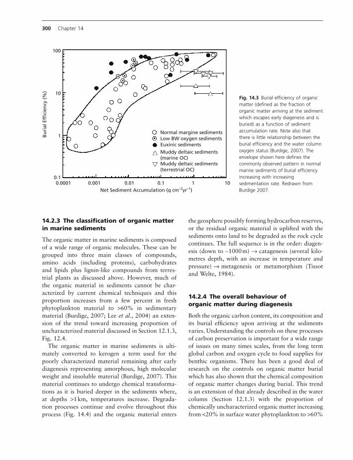
Overall organic matter burial effi ciency, that is, how much of the rain of organic matter to the sedi-ments escapes early diagenesis varies with sediment accumulation rate from <1% in slow sedimentation open ocean regimes to >50% in fast sedimentation delta regimes (Fig. 14.3).

cling. Regardless of the uncertainties in the actual values two striking features are apparent from Table 14.1.

Firstly, considering the open ocean waters ( >2km),in Table 12.3 the fl ux of organic matter through 2000m was estimated at 340 × 1012 gCyr−1, so less than 20% of the carbon passing this depth and reaching the sediments is fi nally buried, illustrating again the effi ciency of carbon recycling throughout the ocean system. Indeed Burdige suggests that the burial effi ciency in waters deeper than 4 km (63% of the ocean area) is <5%.

The second point from Table 14.1 is the domi-nance of shallow water systems, and in fact deltas in particular, in ocean carbon burial.

14.2.2 The sources and distribution of organic matter in marine sediments

The organic matter in marine sediments is derived from terrestrial, marine and anthropogenic sources.

In Chapter 6 the fl uvial and atmospheric fl uxes of organic carbon to the oceans were estimated at 216 and 180 × 1012 gyr−1 respectively, a sum that is only about 1% of the organic carbon produced within the oceans (see Chapter 9) and hence the overall carbon cycle in the oceans is dominated by internal produc-tion by photosynthesis. However, as we have seen only about 1% of ocean primary production reaches the sediments, the rest being degraded while sinking through the water column. By contrast, the external inputs to the oceans, particularly those arriving through the fl uvial system, have already been exten-sively degraded during transport and include mate-rial rather more resistant to degradation. In particular, fl uvial material includes lignin, a phenolic compound forming a major structural element in terrestrial

Table 14.1 Ocean Organic Carbon Burial 10 12 g organic C yr −1.Based on Burdige (2007).

Depth Range (km) % ocean area Organic Carbon Burial (% of total in brackets)

0–0.2 7 152 (50%) 0.2–2 9 96 (31%)

>2 84 61 (20%)

300 Chapter 14

the geosphere possibly forming hydrocarbon reserves, or the residual organic material is uplifted with the sediments onto land to be degraded as the rock cycle continues. The full sequence is in the order: diagen-esis (down to ∼ 1000 m) → catagenesis (several kilo-metres depth, with an increase in temperature and pressure) → metagenesis or metamorphism (Tissot and Welte, 1984 ).

14.2.4 The o verall b ehaviour of o rganic m atter d uring d iagenesis

Both the organic carbon content, its composition and its burial effi ciency upon arriving at the sediments varies. Understanding the controls on these processes of carbon preservation is important for a wide range of issues on many times scales, from the long term global carbon and oxygen cycle to food supplies for benthic organisms. There has been a good deal of research on the controls on organic matter burial which has also shown that the chemical composition of organic matter changes during burial. This trend is an extension of that already described in the water column (Section 12.1.3 ) with the proportion of chemically uncharacterized organic matter increasing from < 20% in surface water phytoplankton to > 60%

14.2.3 The c lassifi cation of o rganic m atter in m arine s ediments

The organic matter in marine sediments is composed of a wide range of organic molecules. These can be grouped into three main classes of compounds, amino acids (including proteins), carbohydrates and lipids plus lignin - like compounds from terres-trial plants as discussed above. However, much of the organic material in sediments cannot be char-acterized by current chemical techniques and this proportion increases from a few percent in fresh phytoplankton material to > 60% in sedimentary material (Burdige, 2007 ; Lee et al. , 2004 ) an exten-sion of the trend toward increasing proportion of uncharacterized material discussed in Section 12.1.3 , Fig. 12.4 .

The organic matter in marine sediments is ulti-mately converted to kerogen a term used for the poorly characterized material remaining after early diagenesis representing amorphous, high molecular weight and insoluble material (Burdige, 2007 ). This material continues to undergo chemical transforma-tions as it is buried deeper in the sediments where, at depths > 1 km, temperatures increase. Degrada-tion processes continue and evolve throughout this process (Fig. 14.4 ) and the organic material enters

Fig. 14.3 Burial effi ciency of organic matter (defi ned as the fraction of organic matter arriving at the sediment which escapes early diagenesis and is buried) as a function of sediment accumulation rate. Note also that there is little relationship between the burial effi ciency and the water column oxygen status (Burdige, 2007 ). The envelope shown here defi nes the commonly observed pattern in normal marine sediments of burial effi ciency increasing with increasing sedimentation rate. Redrawn from Burdige 2007 .

0.0001 0.001

Bu

rial

Eff

icie

ncy

(%

)100

10

1

0.10.01 0.1 1

Normal margine sedimentsLow BW oxygen sedimentsEuxinic sediments

Muddy deltaic sediments(marine OC)Muddy deltaic sediments(terrestrial OC)

10Net Sediment Accumulation (g cm–2yr–1)

Sediment interstitial waters and diagenesis 301

and Keil, 1995 ; Lee et al. , 2004 ). This mechanism may be particularly important in protecting organic matter from degradation (see also Section 12.1.3 ), but reactions on the surfaces of the bound organic matter may change its chemical character.

These mechanisms are not mutually exclusive and all may occur together, or in sequence, during the breakdown of organic matter and the relative impor-tance of each of them may vary between different environments or sediment types (Burdige, 2007 ).

The role of oxygen concentrations in infl uencing organic matter preservation has been extensively dis-cussed. The very limited organic matter preservation in well oxygenated oceanic abyssal sediments and the organic rich sediments underlying an anoxic environ-ment, such as the Black Sea, suggest an important role for oxygen concentration in regulating sediment organic carbon preservation. However, the data in Fig. 14.3 show that burial effi ciency is not par-ticularly closely related to oxygen concentrations.

in the sediments. As Lee et al. (2004) and Burdige (2007) note, this increase in the uncharacterized frac-tion does not necessarily imply the material is any less biodegradable. Burdige (2007) identifi es three processes that play a role in determining burial effi ciency and in this chemical evolution to an organic composition dominated by this uncharacter-ized fraction. 1 Degradation of organic matter produces reactive products that can then react to form this complex uncharacterized material. 2 The bacterial degradation may selectively remove the characterized fraction. 3 The organic matter may be physically protected within, or on, inorganic/organic substrates. The bind-ing of organic matter to surfaces such as clay parti-cles may in itself protect organic matter from degradation, or offer physical protection by trapping material in pore spaces that are suffi ciently small to prevent entry by bacteria and or enzymes (Hedges

Fig. 14.4 Stages in the diagenesis, catagenesis and metagenesis of organic matter in sediments (from Tissot and Welte, 1984 ).

Unalteredmolecules

Livingorganisms Lignin

Carbo-hydrates Proteins Lipids

Microbialdegradation

PolymerizationCondensation

Recentsediment

Fulvic acidsHumic acids

Humin

Kerogen

Geochemical fossils

Releaseof trappedmoleculesThermal

degradation

Principal zoneof oil formation

HydrocarbonsLow to medium MW

HC

High MW

Crude oil

Methane+

Light hydrocarbonsGas

Cracking

Carbon residue

Cracking

Dia

gen

esi

s

Zoneof gas formation

Cata

gen

esi

sM

eta

gen

esi

s

Minor alterationretaining carbon

skeleton

302 Chapter 14

underlain by a turbidite sequence made up of an upper light brownish grey unit and a lower green unit. The sediment had an overall accumulation rate of ∼ 10 cm 10 3 yr − 1 . The organic carbon content was ∼ 0.6% in the surface layer and rose to ∼ 1.6% around the top of the green layer. The interstitial water chemistry of the sediment at this site was consider-ably more complex than that of the exclusively pelagic deposit refl ecting the adjustment of the system to the introduction and subsequent burial of the organic rich turbidite sequence. Wilson et al. (1985) suggested that the sequence could be inter-preted in terms of two zones. Zone 1 is close to the sediment surface refl ecting normal pelagic sedimen-tation in which almost all the organic matter is con-sumed by oxic processes. Below this zone there is a second zone of high diagenetic activity refl ecting the presence of the organic rich turbidite sediments which are oxidized by oxidants diffusing from above. This creates a downward - moving oxidation front, the rate of movement of which is controlled by the rates of diffusion of oxygen and nitrate from the bottom water to the front itself. The progressive downward migration of the turbidite oxidation front is not a steady - state process; rather it implies that there is a continuing readjustment of the redox profi le after the deposition of an organic - rich unit, which initially was at the original pelagic sediment surface.

14.3 Diagenesis: s ummary

1 Early diagenesis in marine sediments follows a general pattern in which a series of oxidants are utilized for the destruction of organic carbon in the following general sequence:

oxygen nitrate manganese oxides

iron oxides sulfate

→ ≅→ → .

The consumption of these oxidants represents an important component of their global biogeochemical cycles. Thus, sedimentary denitrifi cation, particu-larly in shelf, slope and hemipelagic sediments, is responsible for about 60% of the loss of nitrogen from the oceans, with the remainder lost by water column denitrifi cation in low oxygen regions ( ∼ 30%, see Chapter 9 ) and burial of organic matter ( ∼ 10%) (Brandes et al. , 2007 ). Estimated sulfi de burial in

However, the oxygen concentrations in bottom waters are closely related to the organic carbon content of sediments because the breakdown of that organic matter can consume oxygen (Middleburg and Levin, 2009 ). In most sedimentary environ-ments, oxygen is available for the initial degradation of organic matter (Middleburg and Levin, 2009 ), and hence the organic matter degraded by alternative electron acceptors has already been modifi ed from that degraded using oxygen (Middleburg and Levin, 2009 ). Burdige (2007) concludes from an extensive review of the literature that; 1 Fresh labile organic matter is degraded under oxic and anoxic conditions, although the rates may be different. 2 Refractory organic matter may be degraded more slowly, and/or less effi ciently, under anoxic or low oxygen conditions. This may be because the break-down of such refractory material requires oxygen (Middleburg and Levin, 2009 ).

Burdige identifi es two other factors that may be potentially important in regulating organic matter burial. The fi rst is the time that organic matter is exposed to oxygen, a factor that explains the very low organic carbon burial in deep ocean sediments and the effect of burial rate (Fig. 14.3 ). The second factor is that a temporally variable redox environ-ment tends to promote organic matter degradation. Such temporal variability is most likely in shallow water systems and in sediments subject to extensive bioturbation.

The discussion to date has assumed a relatively simple conceptual model in which organic matter falls onto the sediment surface continuously and is steadily and slowly buried. This model is good approximation for most of the oceans most of the time. However, these system may not always be in steady state, and Burdidge (2007) notes that on glacial/interglacial timescales, the nature of continen-tal shelves have changed fundamentally and with that change an important change in the ocean carbon cycle can be anticipated given the current dominance of the shelf seas in organic carbon sedimentation. Wilson et al. (1985) provide another example of non - steady state conditions in a study of the inter-stitial water chemistry of a mixed - layer pelagic – turbidite sediment in the north east Atlantic. This sediment (station 10554) consisted of a thin ( ≤ 10 cm) upper light brownish grey layer of pelagic material,

Sediment interstitial waters and diagenesis 303

ocean, thus setting up a lateral gradient in the diage-netic sequence. As a consequence of this, the diagenetic stage reached drops progressively from (i) nearshore sediments with an anoxic layer close to the sediment surface sometimes only mm from the surface), to (ii) nearshore sediments having a slightly thicker oxic layer, to (iii) hemi - pelagic deep - sea sedi-ments having an oxic layer of a few centimetres followed by zones of nitrate, manganese oxide and iron oxide reduction, to (iv) truly pelagic deep - sea sediments, in which diagenesis does not progress beyond the oxic stage at which oxygen consumes virtually all the organic carbon brought to the sedi-ment surface. In shelf and slope sediments organic matter can be protected at least to some extent by association with sediment surfaces.

During diagenesis elements are mobilized into solution and so can migrate through the interstitial waters. Some of these elements (together with those already present in the interstitial waters) are incor-porated into newly formed or altered minerals.

sediments is equivalent to almost half of the input of sulfate to the oceans (Berner, 1982 ). 2 The diagenetic sequence passes through each of the oxidant utilization stages successively in a down - column direction, thus setting up a vertical gradient. 3 Most organic matter delivered to the oceans and produced within the oceans is degraded within the ocean water column or else on or within the sedi-ments and is not ultimately buried. The degree to which organic matter suffers degradation in marine sediments depends on the rate at which it is degraded versus the rate at which is it buried. Organic carbon burial in the oceans occurs predominantly in deltas and on the continental shelf as illustrated in Fig. 14.5 . 4 The extent to which the diagenetic sequence itself proceeds depends largely on the rate of supply of organic matter to the sediment surface and the rate at which it is buried. Both of these decrease away from the continental margins towards the open -

Fig. 14.5 Idealized diagram depicting estimates of organic matter burial (expressed as a percentage of the total ocean sediment organic carbon burial), in a number of marine environments types (after Hedges and Keil, 1995 ). Reprinted with permission from Elsevier.

Pelagic–5%

Shelf–45%

Abyssal Plain

Rise

Slope

Anoxicbasins<1% Upwelling

lowbottom

waterO2

High productivityzones<6%

Transport

Turbiditeflows

Bypass

Delta44%

304 Chapter 14

However, a fraction of the elements can escape capture in this way, and so be released into the over-lying seawater. In the next section, therefore, the wider aspects of diagenetic mobilization will be considered in relation both to the depletion -enrichment of elements in interstitial waters and to the potential fl uxes of the elements to the oceanic water column.

14.4 Interstitial water inputs to the oceans

14.4.1 Introduction

Early diagenesis takes place generally over the upper tens of centimetres of marine sediments involving the oxidative destruction of organic matter. Reactions continue as the sediment is buried deeper and may involve interactions with underlying basalts. However, rates of exchange of the sediment porewa-ters with the overlying seawater decrease with depth and hence the impacts on ocean water chemistry become less. These early diagentic processes can play an important role in the interstitial water chemistries and oceanic cycling of a number of components. These include the following.1 The bioactive, or labile, elements such as C, N, P, together with Ca (calcium carbonate) and Si (opal). A characteristic of these elements is that only a rela-tively small fraction of their down -column rain rates are preserved in marine sediments, with most of them being recycled. The preservation of organic carbon was discussed earlier and the preservation of carbon-ate and silica are discussed in Chapter 15 since they profoundly affect the major solid components of ocean basin sediments. 2 The oxidants used to destroy organic matter are: oxygen, nitrate, Mn and Fe oxides, and sulfate (see Section 14.1.2). The consumption of nitrate and sulfate within sediments by these reactions is a major term in the global biogeochemical cycles of these ions. 3 Trace metals. Diagenetic processes involved in the oxidative destruction of organic matter are inti-mately related to the interstitial water chemistries of many trace metals, including those transported down the water column by organic carriers and those asso-ciated with the oxidants (e.g. Mn oxides). For metals in associations such as these, the diagenetic destruc-tion of organic matter acts as a recycling term.

4 Refractory elements. Changes also occur during early diagenesis that are not related to the oxidative destruction of organic matter. These changes affect the non -bioactive, or refractory, elements (e.g. Na, K, Mg) and involve reactions with aluminosilicacte mineral phases which create biogeochemical sources for some elements and sinks for others.

The elemental composition of interstitial waters therefore is controlled by a number of interrelated factors, which include:1 the nature of the original trapped fl uid, usually seawater;2 the nature of the water transport processes, that is, convection or diffusion; 3 reactions in the underlying basement, including both high - and low -temperature basalt –seawaterinteractions;4 reactions in the sediment column; 5 reactions across the sediment –seawater interface.

As a result of these reactions, changes can be pro-duced in the composition of the interstitial waters relative to the parent seawater, and diffusion gradi-ents can be set up under which the components will migrate from high - to low -concentration regions. In contrast, under some conditions the compositions of the interstitial water and seawater will not differ signifi cantly and concentration gradients will be absent.

The transport by diffusional processes can be described mathematically and this has allowed the development of some chemical models of sediment pore water processes that are much more sophisti-cated than can be used to describe water column processes. These are illustrated in the worksheets in this chapter.

The sampling of ocean sediment pore waters is usually done by the collection of sediment cores which can be divided into section of a cm in length or less from which pore water can be extracted by fi ltration or centrifugation. Some of the key chemical reactions are very sensitive to temperature and pres-sure and others to the presence or absence of oxygen, so care is required during sampling of pore waters to minimize the effect of changes due to sampling. For a small number of sediment components it is now possible to measure the pore water chemistry in situ using for example electrodes which can be auto-matically lowered into the sediment to increasing depths (Martin and Sayles, 2003).

Sediment interstitial waters and diagenesis 305

could be identifi ed from the data obtained on this transect. 1 The interstitial waters were almost always enriched in Na + , Ca 2 + and HCO3

−, and depleted in K + and Mg 2 + , relative to seawater. In addition, SO4

2− was slightly enriched at most stations, probably refl ecting the role of sulfate as an alternative electron acceptor in organic matter oxidation. 2 The extent of these depletions or enrichments varied from element to element. For example, the enrichments in Na + were relatively small, and although the pore water concentration increased with depth the gradient was only gradual. In contrast, the other major cations had interstitial - water distribution profi les that were characterized by sharp gradients in the upper 15 – 30 cm of the sediments with only a limited change at greater depths. 3 The concentrations of Mg 2 + , K + , Ca 2 + and HCO3

− in the interstitial waters all exhibited a pronounced geographical variability, with the highest concentra-tions being found in waters from the marginal sedi-ments and the lowest in those from the central ocean areas.

It may be concluded therefore that, relative to seawater, the interstitial fl uids of the upper 1 – 2 m of oceanic sediments are generally enriched in calcium, sodium and bicarbonate and are depleted in potassium and magnesium. Some of the processes causing these interstitial - water enrichments and depletions are discussed below, and a number of the basic concepts relating to the behaviour of chemical species in interstitial water are discussed in Work-sheet 14.2 .

The depletion of K + is consistent with its incor-poration into clay minerals as proposed in the reverse weathering concept (Mackenzie and Kump, 1995 ). The formation of interstitial - water gradients can be illustrated with respect to calcium and mag-nesium. Concentration gradients, showing increases in calcium and decreases in magnesium with depth, have been reported in the interstitial waters of many deep - sea sediments. The theories advanced to explain the existence of these gradients include: 1 the formation of dolomite or high - magnesium calcite during the dissolution and recrystallization of shell carbonates, which would account for the interstitial - water gains in calcium and losses in magnesium;

14.4.2 Major e lements

Diagenesis associated with the destruction of organic matter, involving C, N and P, has been described in Section 14.1 , and with respect to the major intersti-tial water constituents, attention in the present section will be confi ned largely to the non - biogenic elements in porewaters. Interest in these components arises from trying to understand the role of chemical processes in sediment burial in creating large scale removal routes for the major ions Na + , K + and Mg 2 + from the oceans. This process is often referred to as reverse weathering and involves the formation within ocean sediments of metal - rich clay material from degraded clays and silica formed during weathering (Mackenzie and Kump, 1995 ). Such processes have now been detected in at least coastal delta sediments and may occur more widely (Michalopoulis and Aller, 1995 ). Reverse weathering was proposed to explain imbalances in global major ion budgets. However, the discovery of the large scale hydrother-mal processes at mid ocean ridges and the role of these systems as sources and sinks for many major ions, suggests that a major role for reverse weather-ing in major ion budgets may not be required, although this issue is far from settled (Mackenzie and Kump, 1995 ).

Analyses of interstitial waters were fi rst carried out more than 100 years ago (see e.g. Murray and Irvine, 1895 ). Until recently, however, data for the chemistry of interstitial water have suffered from a number of major uncertainties. According to Sayles (1979) these arose from: 1 sampling procedures, such as temperature - induced artefacts inherent in the water extraction techniques; 2 imprecise analytical techniques (especially for trace elements); and 3 a lack of detail close to the sediment – seawater interface, a region where a number of important reactions take place.

Because of factors such as these, much of the early interstitial - water data must be regarded as being unreliable. In order to rectify some of these uncer-tainties, Sayles (1979) carried out a study of the composition of interstitial waters collected using in situ techniques from the upper 1 – 2 m of a series of sediments from the North and South Atlantic on a marginal – central ocean transect. A number of trends

306 Chapter 14

Worksheet 14.2: Some b asic c oncepts r elating to the b ehaviour of c hemical s pecies in the s ediment – i nterstitial - w ater c omplex

Interstitial waters are the medium through which elements migrate during diagenetic reactions. In sediments the interstitial - water properties change very much more rapidly in the vertical than in the horizontal direction, with the result that the changes can often be described by one - dimensional models. The transport of solutes through interstitial waters takes place by convection, advection and diffusion. In the context used here advection refers to transport by the physical movement of the water phase, and diffusion refers to migration of a chemical species through the water as a result of a gradient in its concentration (or chemical potential). Diffusion in an aqueous solution can be described mathematically by Fick ’ s laws, which, for one dimension, may be written as follows (see e.g. Berner, 1980 ): 1 First law

J Dcx

i ii= −

∂∂

(WS14.2.1)

2 Second law

∂∂

=∂∂

ct

Dc

xi

ii

2

2 (WS14.2.2)

Here J i is the diffusion fl ux of component i in mass per unit area per unit time, c i is the concentration of component i in mass per unit volume, D i is the diffusion coeffi cient of i in area per unit time, and x is the direction of maximum concentration gradient; the minus sign in the fi rst law indicates that the fl ux is in the opposite direction to the concentration gradient. Fick ’ s fi rst law is applied to calculations that involve steady - state systems, and the second law is applied to non - steady - state systems. Before Fick ’ s laws can be applied directly to sediments, however, it is necessary to take account of the nature of the sediment – interstitial - water complex. Interstitial waters are dispersed throughout a sediment and the rate of diffusion of a solute through them is less than that in water alone, that is, as predicted by Fick ’ s laws, because of the solids present (the porosity effect) and because the diffusion path has to move around the grains; the term tortuosity ( θ ) is used to describe the ratio of the length of the sinuous diffusion path to its straight - line distance (Berner, 1980 ). Tortuosity is usually deter-mined indirectly from measurements of electrical resistivity of sediments and of the interstitial waters separated from them, using the relationship

θ φ2 = F (WS14.2.3)

where ϕ is the porosity and F is the formation factor ( F = R / R 0 , where R is the electrical resis-tivity of the sediment and R 0 is the resistivity of the interstitial water alone). Formation factors in marine sediments usually appear to lie in the range around 1 to around 10, so that the effective diffusion coeffi cient ( D ′ ) in sediment will be less than in the solution alone by a factor of up to around 10. The effective diffusion coeffi cient can be calculated from the relationship

′ =DDφ

θ2 (WS14.2.4)

continued

Sediment interstitial waters and diagenesis 307

where D is the diffusion coeffi cient in solution, ϕ is the porosity and θ is the tortuosity. A detailed treatment of how to apply Fick ’ s laws directly to sediments is given in Berner

(1980) , and for a comprehensive mathematical treatment of migrational processes and chemi-cal reactions in interstitial waters the reader is referred to the ‘ benchmark ’ publication by Lerman (1977) .

To illustrate this approach with an example, Gieskes (1983) has pointed out that if it is assumed that only vertical transport through interstitial waters is important, then the fl ux of a chemical constituent can be described by the equation

J pDcz

pucb b= −∂∂

+ (WS14.2.5)

where J b is the mass fl ux, p is the porosity, z is the depth coordinate in centimetres (positive downwards), u is the interstitial - water velocity relative to the sediment – water interface in cm b s − 1 (i.e. the advection rate), c is the mass concentration in mol cmp

−3 and D b is the diffusion coeffi cient in the bulk sediment (the subscript b indicates that concentrations and distances are measured over the bulk sediment (i.e. solids and interstitial waters) and the subscript p indicates the interstitial water phase only).

The mass balance of the solute is given by

∂∂

=∂∂

( ) +pct z

J Rb (WS14.2.6)

where R is a chemical source – sink term, that is, the reaction rate ( mol cm sb− −3 1).

If the interstitial - water density and the solid density do not change in a given depth horizon, then

∂∂

=∂∂

pt

puz

(WS14.2.7)

and Equation WS14.2.6 becomes

pct z

pDcz

pucz

R∂∂

=∂∂

∂∂

⎛⎝⎜

⎞⎠⎟ −

∂∂

+b (WS14.2.8)

and when steady state exists, this becomes

0 =∂∂

∂∂

⎛⎝⎜

⎞⎠⎟ −

∂∂

+z

pDcz

pucz

Rb . (WS14.2.9)

According to Gieskes (1983) if conditions (e.g. sedimentation rates, temperature gradients) have been stable during relatively recent times (the last 10 – 12 Ma), then the steady - state assumption is valid for pelagic sediments, which have accumulation rates of ∼ 20 m Ma − 1 . The author then considered how a concentration – depth gradient, such as that illustrated in Fig. WS14.2.1 , could be explained.

Gieskes (1983) considered the factors that might control the concentration – depth relation-ship in the dissolved Ca profi le illustrated in Fig. WS14.2.1 and related them to changes in three variables. These variables were diffusion ( D b ), reaction rate ( R ) and advection ( u ); that

continued on p. 308

308 Chapter 14

is, the profi les were interpreted within a diffusion – advection – reaction framework. To illustrate this approach, three cases were considered.

Case 1 , in which the rate of diffusion varies; that is, R = 0, D b = f ( z ) and u = 0. Under these conditions, there is no reaction and no signifi cant contribution from advection. Thus, only a gradual decrease in D b with depth could then explain the increased curvature with depth in the otherwise conservative profi le.

Case 2 , in which the reaction rate varies; that is, R ≠ 0, D b is constant and u = 0. Thus, the profi le implies a removal of calcium from solution, notwithstanding the signifi cant source term for dissolved Ca at the lower boundary.

Case 3 , in which the advection rate is not zero; that is, R = 0, D b is constant and u ≠ 0. Thus, under these conditions of no reaction and constant diffusion coeffi cient, the curvature in the profi le would be caused by the relatively large advective term.

Gieskes (1983) then considered two types of Ca – Mg interstitial - water concentration – depth profi les. In the fi rst type, there are linear correlations between Δ Ca and Δ Mg, that is, R = 0. Using data that included information on porosity, and diffusion coeffi cients (evaluated from a knowledge of formation factors; see above), a solution of Equation WS14.2.9 assuming R = 0 indicated that the depth profi les of Ca and Mg could be explained in terms of conservative behaviour (i.e. transport through the interstitial water column alone and no reaction), with the boundary conditions being fi xed by concentrations in the underlying basalts and the overlying seawater. In the second type, there are non - linear correlations between Δ Ca and Δ Mg, which implies reaction in the sediment column; that is, R ≠ 0. Under these conditions, derivatives of Equation WS14.2.9 must be evaluated geometrically from the concentration – depth profi les in order to model the data. These two types of Ca – Mg profi les are described in the text.

Fig. WS14.2.1 Concentration – depth profi le of dissolved Ca in interstitial waters of a DSDP core (from Gieskes, 1983 ). Reprinted with permission from Elsevier.

Dep

th (

m)

0

100

0Concentration (mM)

200

300

20 40 60

Sediment interstitial waters and diagenesis 309

2 the adsorption of magnesium on to opal phases, which would result in a decrease in magnesium in the interstitial waters of siliceous sediments.

However, in addition to changes in magnesium and calcium there is often a decrease in δ 18 O values in the interstitial waters, and according to Lawrence et al. (1975) this cannot be explained by reactions involving either carbonate or opaline diagenesis. Instead, these authors proposed that the changes in δ 18 O values result from reactions taking place during the alteration either of the basalts of the basement or of volcanic material dispersed throughout the sediment column. The problem was addressed by Gieskes (1983) , who identifi ed two types of calcium – magnesium profi les in the interstitial waters from ‘ long - core ’ oceanic sediments and linked them to reactions involving interstitial waters and volcanic rocks, either in the basalt basement or in the sedi-ment column itself, or in both.

Fig. 14.6 Interstitial water profi les at DSDP sites. Concentration – depth profi les at DSDP site 446 (24 ° 42 ′ N, 132 ° 47 ′ E). Lithology: I, brown terrigenous mud and clay; II, pelagic clay and ash, siliceous; IIIa, mudstone, clay stone, siltstone, sandstone; IIIb, calcareous clay and mudstones, turbidites; IV, calcareous claystones, glauconite, mudstones; V, basalt sills and intrusions. (From Gieskes 1983 .) Reprinted with permission from Elsevier.

200

400

600

02987 4 3020

III

IIIaIIIb

IV

V

Alkalinity(meq l–1)pH

1008060 0210410Sulphate (mM)

200Calcium and magnesium (mM)

Mg Ca

200

400

600

00.20.10 0.3

Strontium (mM)

?

840 12Potassium (mM)

400200 0080Silica (μM)

600

Δ

Ω

Dep

th (

m)

Reactions i nvolving b asement r ocks. Reactions continue deep into the sediments and these can be sampled from sediments collected from the ocean drilling project. Such data is illustrated in Fig. 14.6 . The profi les in Fig. 14.6 are interpreted as showing evidence of a range of geochemical processes. 1 the maximum in the strontium concentrations probably results from the recrystallization of carbon-ates in the nanofossil ooze, during which new mineral phases are formed that have lower strontium concen-trations than the parent material; 2 potassium concentrations decrease with depth, probably as a result of the uptake of the element during the formation of potassium - rich clays; 3 the sulfate profi le shows a decrease with depth, indicating that there has been sulfate reduction within the sediment column; 4 the calcium and magnesium profi les are inter-preted as showing a sink for Mg at depth by reaction

310 Chapter 14

is added directly to seawater. Careful sampling to avoid contamination is required for the analysis of trace metals in porewaters as with the water column (Chapter 11 ). The results of one study of trace metals in sediment pore waters is Fig. 14.7 and the distribu-tion patterns seen here have been seen in other studies. Note that all the four metals considered are enriched in pore waters to some extent relative to seawater. The solubility of manganese is much greater in the Mn(II) form than Mn(IV) and the increase in Mn in porewaters below 15 cm in Fig. 14.7 refl ects the onset of the use of Mn(IV) as an alternative electron acceptor in organic matter oxida-tion. The similar behaviour of Ni suggests that it is associated with manganese oxide phases in sedi-ments and mobilized along with Mn. Cadmium appears to be unaffected by these processes so is presumably not subject to a net fl ux to the interstitial waters through organic matter breakdown in the upper part of the sediment core or during manganese reduction. Copper by contrast is strongly enriched in surface sediment porewaters probably through organic matter degradation and this generates a fl ux of copper into the overlying ocean waters (Boyle et al. ; 1977 , see also Chapter 11 ). The modelling of such sediment pore water profi les is considered in Worksheet 14.3 .

with basalt and an associated source of calcium, although in other profi les detailed modelling suggests additional reactions of these ions occurring within the sediments as well as the deeper basalt interface.

14.4.3 Trace e lements

The fate of a component following deposition in sediments is constrained by its post - depositional mobility, since in order to be added to the interstitial water from solid sediment phases it must fi rst be solubilized to the dissolved state. For many trace metals this solubilization is intimately related to the oxidative destruction of organic matter during early diagenesis. The trace metals that are released in this process to become concentrated in interstitial waters relative to overlying seawater can follow one of two general pathways: 1 they can be released (i.e. recycled) back into sea-water via upward migration across the sediment – water interface; 2 they can be reincorporated into sediment compo-nents following upward or downward migration through the interstitial waters.

Thus, it is necessary to introduce the concept of a net interstitial water fl ux, which in the present context is the fl ux that escapes reaccumulation and

Fig. 14.7 Interstitial - water profi les of dissolved trace metals (from Klinkhammer et al. , 1982 ) from a sediment core that was in a suboxic condition below an oxic surface layer. Arrowheads indicate the bottom water concentrations. Reprinted with permission from Elsevier.

Dep

th (

cm)

Dissolved metal concentration (nmoles kg–1)

4000

30

0 200

10

20

2000Manganese

1000 50Nickel

300 15Cadmium

3000 100Copper

200

Sediment interstitial waters and diagenesis 311

Worksheet 14.3: Models for the r egeneration of t race m etals in o xic s ediments

Klinkhammer et al. (1982) reported data on the concentrations of Ni, Cd and Cu in bottom waters and oxic sediment interstitial waters at MANOP site S in the central equatorial Pacifi c, and used these to set up diagenetic models. A characteristic feature of the metal interstitial - water profi les at the oxic site (S) is that the steepest concentration gradient is found across the sediment – seawater interface, which implies that most metal regeneration in these oxic sedi-ments takes place across this interface. The concentration – depth profi les are maintained by a combination of the regeneration and the interaction between the dissolved metals and the sediment below the interface. Nickel and Cd exhibit little tendency to react with sediment components under these conditions, with the result that their interstitial water profi les are monotonic at site S and are generated by the burial of surfi cial pore water. In contrast, Cu is readily taken up by sediment components, which leads to an exponential decrease in interstitial - water dissolved Cu concentrations with depth: see Fig. WS14.3.1 .

Ni and Cd r egeneration Under conditions of oxic diagenesis the degradation of organic matter in surface sediments utilizes dissolved oxygen, and Klinkhammer et al. (1982) assumed that in the simplest case early oxic diagenesis on the sea fl oor is analogous to oxidation in the overlying water column, that is, a ‘ continuum model ’ . Nickel and Cd are nutrient - type elements in seawater so that under oxic conditions it should be possible to predict the Ni and Cd concentrations in the surfi cial interstitial waters from the interstitial nutrient concentrations. To set up a model for

Fig. WS14.3.1 Dissolved metal concentrations in the interstitial waters of oxic sediments at MANOP site S (nmol l − 1 ). Arrow heads indicate bottom - water concentrations.

Dep

th (

cm)

20

30

0

10

20

10Nickel

200 10Cadmium

500 25Copper

continued on p. 312

312 Chapter 14

this, Klinkhammer et al. (1982) assumed that both the metals and the nutrients are lost from the sediment – seawater interface by diffusion only, so that the fl ux of metal M across the inter-face is related to the corresponding fl ux of a nutrient N by a proportionality constant M/N . Thus

DMz

MN

DNz

Mz

Nz

dd

dd

⎛⎝⎜

⎞⎠⎟ = ⎛

⎝⎜⎞⎠⎟= =0 0

. (WS14.3.1)

By assuming a linear concentration gradient across the interface, Equation (WS14.3.1) reduces to the relationship

MN

M M DN N D

M

N

=−−

( )( )

.0

0

BW

BW (WS14.3.2)

In the water column Ni mimics silica and Cd is related to nitrate (see Chapter 11 ), and using data from the literature the appropriate diffusion coeffi cient ratios ( D ) were calculated to be D Cd / D NO3 = 0.36 and D Ni / D Si = 0.68. Variables M 0 and M BW are metal concentrations in the top interstitial - water interval and bottom seawater, and N 0 and N BW are the corresponding nutrient concentrations. A comparison of the results obtained from Equation WS14.3.2 with the ratios found in seawater is a test of the model. Klinkhammer et al. (1982) made such a comparison and the data from site S are reproduced in Table WS14.3.1 , and strongly support the ‘ continuum model ’ .

Cu r egeneration Copper is readily taken up by sediment components, which leads to an exponential decrease in interstitial - water dissolved Cu concentrations with depth. In addition, dissolved Cu is released into seawater at the interface. The amount of Cu released in this way, however, is considerably greater than that which would be predicted from the decomposition of organic material consisting of plankton. Thus, the model developed for Ni and Cd is inappropriate for Cu. Klinkhammer et al. (1982) therefore assumed that the interstitial - water dissolved Cu profi les are sustained by scavenging from the water column combined with vigorous recycling at the interface and uptake into the sediment. The authors then attempted to model the interstitial - water dissolved Cu profi le in the following manner.

The shape of the interstitial - water dissolved Cu profi le at site S (see Fig. WS14.3.1 ) shows a concentration gradient that indicates diffusion upwards (into seawater) and downwards (into the sediment) from the interface, and the negative curve suggests an uptake by the sediment at depth. The authors concluded that the simplest model consistent with this type of profi le

Table WS14.3.1 Metal: nutrient ratios (Ni : Si and Cd : NO 3 ) at site S calculated from Equation WS14.3.2 compared with those observed in general sea water and bottom water at the site (from Klinkhammer et al. , 1982 ).

Element ( M : N ) site S × 10 5 ( M : N ) SW × 10 5 ( M : N ) BW × 10 5

Ni 3.2 3.3 5.3 Cd 3.3 2.3 1.8

continued

Sediment interstitial waters and diagenesis 313

was a steady - state approach in which the Cu is controlled by diffusion and fi rst - order removal, which can be represented by the Equation:

DCz

kC∂∂

− =2

20. (WS14.3.3)

The solution of Equation WS14.3.3 for a one - layer sediment is given by

CC h z C Rz

Rh=

− +1 2sinh[( )] sinh( )sinh( )

(WS14.3.4)

where R = ( k/D ) 1/2 , C is the concentration predicted at depth z , C 1 and C 2 are the concentra-tions at the upper ( z = 0) and lower ( z = h ) boundaries, D is the diffusion coeffi cient corrected for porosity, tortuosity and temperature ( D = 1.4 × 10 − 6 cm s − 1 ), and k is the reaction constant in s − 1 . Values for k were calculated using a best - fi t approach. The authors modelled their data to a depth of ∼ 15 cm in the sediment, below which there is little variation. The results for site S are illustrated in Fig. WS14.3.2 . It is apparent from Fig. WS14.3.2 that there is very good agreement between the predicted and observed dissolved Cu interstitial - water profi les, that is, the profi les are adequately explained by the remobilization of Cu at the interface and its removal into the sediment below.

Fig. WS14.3.2 Dissolved Cu interstitial - water profi les in the oxic sediments at site S. Filled circles are the measured concentrations in the interstitial waters. The full curve indicates the curve derived from Equation WS14 .3.4 using the following parameters: C 1 = 47 nmol kg − 1 , C 2 = 26 nmol kg − 1 , h = 13 cm and k = 0.17 yr − 1 .

Dep

th (

cm)

50

30

0

10

20

10Copper (nmoles kg–1)

20 40300

314 Chapter 14

in the composition of the interstitial waters relative to the parent seawater, and diffusion gradients are set up via which elements migrate from high - to low - concentration regions. 4 The most intense reactions usually take place in the upper ∼ 30 – 50 cm of the sediment column. These reactions are in response to the diagenetic environ-ment, the intensity of the reactions generally decreas-ing in the order highly reducing shelf sediments > hemi - pelagic sediments > pelagic sediments refl ect-ing the supply of organic matter. 5 Data are now available on the diffusive interstitial water fl uxes of a number of major and trace compo-nents. For some of these components interstitial waters act as sinks for their removal from seawater; for others they act as sources for their addition to seawater. 6 When considering interstitial water sources it is extremely important to make a distinction between primary and secondary fl uxes. Interactions that take place between the basalt basement and interstitial waters, and between some types of dispersed vol-canic material and interstitial waters, can lead to dissolved components being introduced into seawa-ter for the fi rst time. These are the primary fl uxes in the same way as hydrothermal fl uxes are primary in nature. In contrast, a large fraction of the trace metals that are mobilized into interstitial waters from particulate material via the diagenetic sequence has already been taken out of solution in seawater in the biogeochemical cycles that operate in the water column, and so is simply being returned to the dis-solved state. These are the recycled or secondary fl uxes. The dissolved trace metals associated with these fl uxes can sometimes impose ‘ fi ngerprints ’ on the water column if they escape recapture at the sedi-ment surface. However, the important point is that they have been recycled within the ocean system, and as such do not represent an additional primary exter-nal source. Despite this, the diagenetic remobiliza-tion and release of elements that are initially removed from solution by incorporation into estuarine and coastal sediments can sometimes reverse the pro-cesses that occur in estuaries, and Bruland (1983) has suggested that for these elements such a diagenetic release can be regarded as an ‘ additional dissolved river input ’ to the oceans.

The diagenetic reactions that take place both within the sediment – interstitial - water complex and

As is clearly evident from the Mn profi le in Fig. 14.7 , the redox environment can profoundly affect the cycling of trace metals in porewaters and these affects depend on the chemical characteristics of each element. Morford and Emerson (1999) suggest for instance that Mo and V are released from sediment solid phases along with Mn, whereas overall Re, Cd and U fl ux into the sediments because either they are less soluble in the reduced form (Re and U exist as anions in oxygenated seawater see Chapter 11 ) or because they form very insoluble sulfi des.

Mobilization under reducing conditions within sediment porewaters will only result in release to the water column if the onset of reducing conditions is at or near the sediment surface.

Manganese. The sedimentary geochemistry of man-ganese has attracted considerable interest because of its role within the redox cycle and the impact of this cycle on the solubility of Mn in pore waters. The reactions involved in the diagenesis of Mn can be related to interstitial - water - phase – solid - phase changes, and can be expressed in a simple form as:

Mn soluble MnO solid hydrous oxireductionoxidation

2+ ← →⎯⎯⎯( ) (x dde) (14.7)

where x generally is less than 2. This reaction governs the diagenetic mobility of Mn in sediments, and the general conditions that control both the solid - phase and dissolved Mn in the sediments. The mobilization of Mn at depth in the sediments results in increases in pore water concentrations and upward diffusion of Mn toward the oxic layer where it can reprecipi-tate resulting in a maximum in solid phase Mn within the sediments. This process has been described by a number of models. One of which is described in Worksheet 14.4 .

14.5 Interstitial w ater i nputs to the o ceans: s ummary

1 The interstitial waters of most oceanic sediments originate as trapped seawater. 2 The external boundary conditions for the interstitial - water – sediment complex are set by the basalt basement below and the water column above. 3 Reactions take place in the sediment – interstitial - water sandwich, during which changes are produced

Sediment interstitial waters and diagenesis 315

Worksheet 14.4: The B urdige - G ieskes m odel for the s teady - s tate d iagenesis of M n in m arine s ediments

Burdige and Gieskes (1983) outlined a steady - state pore - water – solid - phase diagenetic model for Mn in marine sediments. The model has been described qualitatively in the text, and also can be used to illustrate how diagenetic equations are used. The Burdige - Gieskes steady - state diagenetic model, which involves a series of Mn reaction zones, is illustrated in Fig. WS14.4.1 .

The derivation of the diagenetic equations used to translate this into a quantitative math-ematical model is summarized in the following.

Burdige and Gieskes (1983) presented a mathematical treatment of their Mn ‘ zonation model ’ using the steady - state diagenetic equations given by Berner (1980) :

DC

zw

C

zR zb

p p∂∂

−∂∂

+ ( ) =2

20 (WS14.4.1)

−∂∂

−−

( ) =wCz

R zs φφ1

0 (WS14.4.2)

where D b is the bulk sediment diffusion coeffi cient (identical with Berner ’ s D s term), C p is the concentration of Mn in the pore waters, C s is the concentration of Mn in the solid phase, w is the sedimentation rate, ϕ is the porosity and R ( z ) is a rate expression for either oxidation or reduction. The term ϕ /(1 × ϕ ), which has units cm 3 porewater / cm 3 dry sed, is used to convert Mn concentrations between the solid and liquid phases.

With respect to the Mn model the following assumptions are implicit in the diagenetic equations. 1 Steady - state diagenesis operates. 2 Vertical gradients are much more important than horizontal gradients, to the extent that the latter can be ignored.

Fig. WS14.4.1 Manganese steady - state diagenetic zonation model (from Burdige and Gieskes, 1983 ).

Oxidized zone (Mn+2 ≈ 0)

Z = 0

Z = L1

Z = L2

sed–water interface

Sea water

Mn-oxidation zone (Mn+2 MnOx)

Mn-reduction zone (MnOx Mn+2)

Equilibrium zone (Mn+2 MnCO3(?))

Z = L3

redox boundary

continued on p. 316

316 Chapter 14

3 Diffusion in pore waters occurs via molecular processes, that is, the diffusion follows Fick ’ s laws. 4 Porosity and diffusion coeffi cients are constant with depth. 5 Advection is constant and equal to the sedimentation rate. 6 Solid - phase diffusion can be neglected. 7 The supply of solid Mn to the sediment surface is constant with time. 8 Adsorption of Mn 2 + can be neglected. 9 Bioturbation can be neglected because in most oceanic sediments it will be confi ned to the well oxygenated layer of sediments above the Mn reduction zone. The authors also drew attention to two other factors, which are detailed in the following.

Variable D b differs from the free - ion diffusion in seawater ( D ) because of tortuosity effects result-ing from the presence of sediment particles, and D b can be related to D by the following equation:

D D Fb = φ (WS14.4.3)

where F is a ‘ formation factor ’ , which is measured as the ratio of the bulk sediment resistivity to the pore - water resistivity (see Worksheet 14.3 ).

In Equations WS14.4.2 and WS14.4.3, R ( x ) is the rate expression for either oxidation or reduction. In the presence of an abundant surface area (such as that of a sediment), Mn precipitation – oxidation is a pseudo - fi rst - order process, so that

R z k Cox ox p( ) = (WS14.4.4)

and Equation WS14.4.5 therefore should be an appropriate rate expression for oxidation under these conditions, in which the reaction product is assumed to be a hydrous oxide (MnO x : see text). The authors assumed that whatever the mechanism involved, the rate of Mn reduction will be proportional to the amount of solid Mn available (which is presumed to be all hydrous oxide). Thus, R red ( z ) can be expressed as

R z k Cred red s( ) .= (WS14.4.5)

Combining the rate expressions with Equations WS14.4.1 and WS14.4.2, the following set of equations was obtained: 1 For the oxidizing zone ( L 1 ≤ z ≤ L 2 )

DC

zw

C

zk Cb

pox

pox

ox pox∂

∂−

∂∂

− =2

20 (WS14.4.6)

−∂

∂+

−=w

Cz

k Csox

ox poxφ

φ10 (WS14.4.7)

2 For the reducing zone ( L 2 ≤ z ≤ L 3 )

DC

zw

C

zk Cb

pred

pred

red sred∂

∂−

∂∂

+−

=2

2

10

φφ

(WS14.4.8)

−∂

∂− =w

Cz

k Csred

red sred 0 (WS14.4.9)

By defi ning a series of boundary conditions the solutions to Equations WS14.4.6 – WS14.4.9 were given as

continued

Sediment interstitial waters and diagenesis 317

C A z Lpox = −( )[ ]sinh α 1 (WS14.4.10)

C GEw

k Dz Lp

red

red b

= −−

− −( )[ ]1 2

2φ

φβexp (WS14.4.11)

C C z Lsox

so= −( )[ ]cosh α 1 (WS14.4.12)

C E z Lsred = − −( )[ ]exp β 2 (WS14.4.13)

where

α = ( )k Dbox1 2 (WS14.4.14)

(assuming 4 D b k ox >> w 2 , i.e. advection in pore waters is negligible compared with diffusion) and

β = k wred (WS14.4.15)

L L Lox = −2 1 (WS14.4.16)

Fig. WS14.4.2 Theoretical models for Mn diagenesis in marine sediments. (a) Model for porewater (broken curve) and solid - phase (full curve) Mn profi les (from Burdige and Gieskes, 1983 ). Profi les predicted from Equations WS14.4.10 to WS14.4.19 using the following parameters: D b = 71.6 cm 2 yr − 1 , w = 3 cm 10 3 yr − 1 , ϕ = 0.8, ρ = 2.6 cm − 3 of sediment, L 1 = 20 cm, L 2 = 30 cm, C o s = 0.1 wt%, k ox = 5 yr − 1 , and k red = 1.50 × 10 − 3 yr − 1 . (b) Schematic representation of model predicted by Froelich et al. (1979) . Reprinted with permission from Elsevier.

Dep

th (

cm)

60

20

40

0.01Mn+2, mM

0.02

0.2Mns, wt %

0.60.4

(a)

continued on p. 318

318 Chapter 14

AC w

D=

−( )so

b

1 φφα

(WS14.4.17)

E C L= ( )so

oxcosh α (WS14.4.18)

G A L L= ( ) + ( )[ ]sinh coshα α β αox ox (WS14.4.19)

There are two unknowns ( k ox and k red ) in the equation, which can be used for a least - squares fi t of the equations to actual data.

By inserting typical parameters for marine sediments into the equations the authors derived model profi les for the diagenesis of dissolved and solid - phase Mn. These are illustrated in Fig. WS14.4.2 (a), and show close agreement with the diagrammatic representation suggested by Froelich et al. (1979) : see Fig. WS14.4.2 (b).

The Mn post - depositional migration associated with this model may be summarized as follows (see text for detailed explanation). As the sediments are buried below the redox bound-ary, solid Mn oxides are reduced to Mn 2 + , which diffuses upwards along the concentration gradient to be oxidized and reprecipitated. With further sedimentation, these reprecipitated oxides are again brought to the reducing zone to be redissolved, with the net result being the Mn trap at the narrow zone at the redox boundary.

Burdige and Gieskes (1983) also applied their equations to solid and porewater data from two cores in the eastern Equatorial Atlantic and obtained very good fi ts to the data.

Dep

th

(b)

(Mn2+)AQ

Manganese concentration

(MnO2)S

Fig. WS14.4.2 Continued

Sediment interstitial waters and diagenesis 319

at the seawater –sediment interface can strongly modify the composition of the material that reaches the sediment reservoir. The nature of these reactions has now been described, and in the following chapter we will consider the composition of the components that form the oceanic sediments in terms of their genetic histories, which, for some material, includes diagenetic modifi cation.

References

Bender , M.L. and Heggie, D.T. ( 1984) Fate of organic carbon reaching the deep sea fl ow: a status report .Geochim. Cosmochim. Acta, 48, 977–986.

Berner , R.A. ( 1980) Early Diagenesis: A Theoretical Approach. Princeton, NJ : Princeton University Press .

Berner , R.A. ( 1981) A new geochemical classifi cation of sedimentary environments . J. Sed. Petrol., 51, 359–365.

Berner , B.A. ( 1982) Burial of organic carbon and pyrite sulfur in the modern ocean: its geochemical and environ-mental signifi cance . Am J. Sci., 282, 451–473.

Boyle, E.A., Sclater , F.R. and Edmond, J.M. ( 1977) Thedistribution of copper in the Pacifi c . Earth Planet. Sci. Lett., 37, 38–54.

Brandes, J.A., Devol, A.H. and Deutsch, C. ( 2007) Newdevelopments in the marine nitrogen cycle . Chem. Rev.,107, 577–589.

Bruland, K.W. ( 1983) Trace elements in sea water , in Chem-ical Oceanography, J.P. Riley and R. Chester (eds), Vol. 8, pp. 156–220. London: Academic Press .

Burdige, D.J. and Gieskes, J.M. ( 1983) A pore water/solid phase diagenetic model for manganese in marine sedi-ments. Am. J. Sci., 283, 29–47.

Burdige, D.J. ( 2007) Preservation of organic matter in marine sediments: controls, mechanisms and an imbal-ance in sediment organic carbon budgets? Chem. Rev.,107, 467–485.

Calvert, S.E. ( 1976) The mineralogy and geochemistry of near -shore sediments , in Chemical Oceanography, J.P. Riley and R. Chester (eds), Vol. 6, pp. 187–280. London:Academic Press .

Calvert, S.E. and Price, N.B. ( 1970) Minor metal contents of Recent organic -rich sediments off South West Africa .Nature, 227, 593–595.

Drever , J.I. ( 1982) The Geochemistry of Natural Waters.Englewood Cliffs, NJ : Prentice-Hall.

Froelich, P.N. , Klinkhammer , G.P. , Bender , M.L. et al.(1979) Early oxidation of organic matter in pelagic sedi-ments of the eastern equatorial Atlantic: suboxic diagen-esis. Geochim. Cosmochim. Acta, 43, 1075–1090.

Galoway , F. and Bender , M. ( 1982) Diagenetic models of interstitial nitrate profi les in deep -sea suboxic sediments .Limnol. Oceanogr., 27, 624–638.

Gieskes, J.M. ( 1983) The chemistry of interstitial waters of deep sea sediments: interpretations of deep -sea drilling data, in Chemical Oceanography, J.P. Riley and R.Chester (eds), Vol. 8, pp. 221–269. London: AcademicPress.

Hedges, J.I. and Keil, R.G. ( 1995) Sedimentary organic matter preservation: an assessment and speculative syn-thesis. Mar. Chem., 49, 81–115.

Klinkhammer , G., Heggie, D.T. and Graham, D.W. ( 1982)Metal diagenesis in oxic marine sediments . Earth Planet. Sci. Lett., 61, 211–219.

Lawrence, J.R., Gieskes, J.M. and Broecker , W.S. ( 1975)Oxygen isotope and carbon composition of DSDP pore waters and the alteration of Layer II basalts . EarthPlanet. Sci. Lett., 27, 1–10.

Lee, C., Wakeham , W. and Arnosti, C. ( 2004) Particulateorganic matter in the sea: the composition conundrum .Ambio, 33, 565–575.

Lerman, A. ( 1977) Migrational processes and chemical reactions in interstitial waters , in The Sea, E.D. Gold-berg, I.N. McCave, J.J. O’Brien and J.H. Steele (eds), Vol. 6, pp. 695–738. New York : John Wiley & Sons, Inc .

Lyle , M. ( 1983) The brown -green color transition in marine sediments: a marker of the Fe(II) –Fe(III) redox boundary .Limnol. Oceanogr., 28, 1026–1033.

Mackenzie, F.T. and Kump, L.R. ( 1995) Reverse weather-ing, clay mineral formation and oceanic element cycles .Science, 270, 586–587.

Martin, W.R. and Sayles, F.L. ( 2003) The recycling of biogenic material at the seafl oor , in Treatise on Geo-chemistry, H.D. Holland and K.K. Turekian (eds), Vol. 7, Sediments, Diagenesis, and Sedimentary Rocks,F.T. Mackenzie (ed.), pp. 37–65. Oxford: ElsevierPergamon.

Michalopoulis, P. and Aller , R.C. ( 1995) Rapid clay mineral formation in Amazon delta sediments: reverse weathering and oceanic elemental cycles . Science, 270, 614–617.

Middleburg, J.J. and Levin, L.A. ( 2009) Coastalhypoxia and sediment biogeochemistry . Biogeosciences,6, 1273–1293.

Morford, J. and Emerson, S. ( 1999) The geochemistry of redox sensitive trace metals in sediments . Geochim. Cos-mochim. Acta, 69, 521–532.

Muller , P.J. and Mangini, A. ( 1980) Organic carbon decom-position ratio in sediments of the Pacifi c manganese nodule belt dated by 230Th and 231Pa. Earth Planet. Sci. Lett., 51, 96–114.

Murray , J. and Irvine, R. ( 1895) On the chemical changes which take place in the composition of the seawater associated with blue muds on the fl oor of the ocean .Trans. R. Soc. Edinburgh, 37, 481–507.

Oremland, R.S. and Taylor , B.F. ( 1978) Sulfate reduction and methanogenesis in marine sediments . Geochim. Cos-mochim. Acta, 42, 209–214.

Roussel, E.G. et al. ( 2008) Extending the sub -sea fl oor biosphere. Science, 320, 1046.

320 Chapter 14

Sayles, F.L. ( 1979) The composition and diagenesis of inter-stitial solutions – I. Fluxes across the seawater –sedimentinterface in the Atlantic Ocean . Geochim. Cosmochim. Acta, 43, 527–545.

Seiter , K., Hensen, C., Schröter , J. and Zabel, M. ( 2004)Organic carbon content in surface sediments – defi ning regional provinces . Deep-Sea Res. I, 2001–2026.

Soetart, K., Herman, P.M.J. and Middelburg, J.J. ( 1996) Amodel of diagenetic processes from the shelf to abyssal depths. Geochim. Cosmochim. Acta., 60, 1019–1040.

Stumm, W. and Morgan, J.J. ( 1996) Aquatic Chemistry. Chemical Equilibria and Rates in Natural Waters. NewYork : John Wiley & Sons, Inc .

Tissot , B.P. and Welte , D.H. ( 1984) Petroleum Formation and Occurrence. Berlin: Springer -Verlag .

Wilson , T.R.S. , Thompson, J., Colley , S., Hydes, D.J. and Higgs, N.C. ( 1985) Early organic diagenesis: the signifi -cance of progressive subsurface oxidation fronts in pelagic sediments . Geochim. Cosmochim. Acta, 49,811–822.