Structure-Based Virtual Screening in Spark

Marco Capuccini

Degree project in bioinformatics, 2015Examensarbete i bioinformatik 45 hp till masterexamen, 2015Biology Education Centre and Department of Pharmaceutical Biosciences, Uppsala UniversitySupervisor: Ola Spjuth

MSc BIOINF 15 005

Abstract

Structure-Based Virtual Screening (SBVS) is a method used in drugdiscovery in order to search leads for certain target receptors. In thepast decades high-throughput methods were used in order to build hugemolecular libraries. ZINC and eMolecules are two high-throughput vir-tual molecular libraries that count million of molecules. Therefore, SBVSis computationally heavy for such libraries. However, SBVS is a triv-ially parallelizable task. In the past Message Passing Interface (MPI)has been used in order to parallelize SBVS. The main disadvantage ofMPI based SBVS is that organizations need High Performance Comput-ing (HPC) facilities in order to run it. Furthermore, MPI does not offermuch more than a message passing interface. Therefore, MPI-applicationsare difficult to implement and maintain. Big data analytics on inexpen-sive hardware was pioneered by Google’s MapReduce programming modeland parallel implementation. MapReduce applications have the propertyto be out of the box fault tolerant and scalable. Therefore, these appli-cations are suitable to run in the cloud, which is in general cheaper thanHPC. Even if Google’s MapReduce is legacy, many open source imple-mentations such as Apache Hadoop are available. However, MapReduceis not a general purpose programming model and does not easily apply toSBVS. The Spark framework is an open source project, and it representsan evolution of Google’s MapReduce. The Spark programming model ismore flexible than MapReduce and it gracefully applies to SBVS. Further-more, Spark-applications are still out of the box fault tolerant, scalableand cloud runnable. Using Spark we implemented a tool for massivelyparallel SBVS. Our tool allows the user to define cloud-ready pipelinesfor high-throughput SBVS with few lines of code. The tests we performedin our private cloud show that our tool is simple to use and it scales well.Therefore, here we show how Spark can be used for massively parallelpipelining, and more in general how Big Data analytics can be beneficialin life science.

Structure-Based Virtual Screening in Spark

Popular science summary

Marco Capuccini

We live in the Big Data era. While producing and storing data is becomingcheaper and faster, we still have the problem of extracting meaningful informa-tion from it in reasonable time. Internet and social networks mostly account forthe data storage and processing demand. For instance, YouTube statistics pressreports that 300 hours of new video are uploaded every minute in its infrastruc-ture. The need of processing such huge datasets represents a new challenge incomputer science, and it makes obsolete all of the data analytics methods thatwe used to adopt.

Only in 2008, Google was already able to process 20 thousand terabytes per day.In order to do so, Google introduced the MapReduce (MR) parallel computingmodel. Instead of relying on expensive hardware, MR manages hardware failuresand minimizes the network communication at software level. Therefore, the MRapplication can run on inexpensive computer clusters, reducing the cost of dataanalitycs.

Spark is an open source project that represents an evolution of Google’s MR.It provides a more flexible programming model, allowing to solve a broaderrange of problems in distributed fashion. Furthermore, Spark applications stillmanage hardware faults and minimize network communication on software level,allowing to use cheap hardware.

Structure-based virtual screening (SBVS) is an in silico method that is aimed tosearch leads for a target receptor in a virutal molecular library. High-throughputmethods in structural biology allowed to produce massive molecular libraries inthe past decade. Therefore, since those libraries contain tens of millions ofmolecules, SBVS can nowadays be seen as a Big Data analytics problem.

In this study we developed a tool for SBVS in Spark. Furthermore, perform-ing some experiments in our private cloud, we showed that Spark-based SBVSscales well. This open-ups SBVS to those organizations that do not own highperformance computer facilities. For instance, an organization could start byusing a small library and few cloud resources, and then scale to lot of cloudresources and high-throughput libraries as the business grows.

Degree project in Bioinformatics, Master of Science (2 years), 2015Biology Education Center and Department of Pharmaceutical BiosciencesSupervisor: Ola Spjuth

Contents

Abbreviations 6

1 Introduction 7

2 Aims 8

3 Background 93.1 Structure-Based Virtual Screening . . . . . . . . . . . . . . . . . 93.2 Big Data analytics . . . . . . . . . . . . . . . . . . . . . . . . . . 103.3 MapReduce . . . . . . . . . . . . . . . . . . . . . . . . . . . . . . 11

3.3.1 Consensus problem in MapReduce . . . . . . . . . . . . . 113.3.2 MR open source ecosystem . . . . . . . . . . . . . . . . . 133.3.3 MR limitations . . . . . . . . . . . . . . . . . . . . . . . . 13

3.4 Apache Hadoop . . . . . . . . . . . . . . . . . . . . . . . . . . . . 143.4.1 HDFS: Hadoop Distributed File System . . . . . . . . . . 143.4.2 YARN: Yet Another Resource Negotiator . . . . . . . . . 14

3.5 Spark . . . . . . . . . . . . . . . . . . . . . . . . . . . . . . . . . 153.5.1 RDD: Resilient Distributed Dataset . . . . . . . . . . . . 153.5.2 Shared variables . . . . . . . . . . . . . . . . . . . . . . . 163.5.3 Consensus problem in Spark . . . . . . . . . . . . . . . . . 163.5.4 Spark SQL and Spark MLlib . . . . . . . . . . . . . . . . 173.5.5 Why Spark for SBVS . . . . . . . . . . . . . . . . . . . . 18

3.6 Cheminformatics . . . . . . . . . . . . . . . . . . . . . . . . . . . 183.6.1 Molecular representations: SMILES and SDF . . . . . . . 183.6.2 Molecular libraries: ZINC and eMolecules . . . . . . . . . 193.6.3 OpenEye toolkits . . . . . . . . . . . . . . . . . . . . . . . 19

4 Implementation 214.1 Programming model . . . . . . . . . . . . . . . . . . . . . . . . . 214.2 Implementation details . . . . . . . . . . . . . . . . . . . . . . . . 22

5 Examples 235.1 Standardization pipeline . . . . . . . . . . . . . . . . . . . . . . . 235.2 Screening pipeline . . . . . . . . . . . . . . . . . . . . . . . . . . 24

6 Materials and methods 26

7 Results 28

8 Discussion and conclusion 31

References 32

Abbreviations

AM Application ManagerAPI Application Programming interfaceCLI Command Line InterfaceDBMS Database Management SystemDN Data NodeHDFS Hadoop Distributed File SystemHPC High Performance ComputingHTS High-throughput screeningMPI Message Passing InterfaceMR Map ReduceNGS Next-Generation SequencingNM Node ManagerNN Name NodePDB Protein Data BankRAM Random Access MemoryRDD Resilient Distributed Data SetRM Resource ManagerSBVS Structure-Based Virtual ScreeningUI User InterfaceVM Virtual MachineYARN Yet Another Resource Manager

6

1 Introduction

High-throughput methods in structural biology allowed to produce massive vir-tual molecular libraries in the past decades. ZINC [1] and eMolecules [2] aretwo well-known examples of that. Since these libraries contain millions ofmolecules, using them in structure-based virtual screening (SBVS) is compu-tationally heavy. However, SBVS is a trivially parallelizable task. Many toolssuch as Multilevel Parallel Autodock4.2 [3] and OEDocking [4] use MessagePassing Interface (MPI) [5] in order to parallelize SBVS. Using MPI has somemajor disadvantages. First, organizations that wish to run MPI based SBVSneed to reserve some running time on an high performance computing (HPC)cluster. This is in general more expensive than buying cloud resources. Fur-thermore, MPI does not offer much more than a message passing ApplicationProgramming Interface (API). This means that problems like data distribution,locality-aware scheduling, load balance, fault tolerance and scalability must behandled by the developers.

Big data analytics on inexpensive hardware was pioneered by Google’s MapRe-duce (MR) [6]. In MR-programming model, data distribution, locality-awarescheduling, load balance, hardware faults and scalability are handled by theMR framework. This makes MR applications able to run in the cloud, wherevirtual machines (VMs) are more likely to fail and network communication isslow. Even though Google’s MR-implementation is legacy, many other imple-mentations are available in the open source ecosystem. Apache Hadoop [7] iswith no doubt the most used open source MR-implementation. Even if Hadoopoffers all of the features of Google’s MR, it has some disadvantages. First, thereis no support for workflows in Hadoop. This means that in order to set upa pipeline some third party tools such as Spotify Luigi [8], or Apache Pig [9]need to be used. In additon, even if newer versions support dataset caching foriterative tasks, Hadoop still lacks broadcast variables support.

Spark is a cluster-computing framework that implements MR, allows in-memoryiterative tasks and has built-in workflow support [10]. Furthermore, Spark of-fers several additional features such as global variables, global sort, machinelearning, and more. We believe that MR and in particular Spark for SBVS aremore flexible and scalable solutions if compared to MPI implementations. Fur-thermore, an in-cloud solution is particularly appealing to those organizationsthat can not access HPC resources, or that just want to try out SBVS and laterscale to high-throughput molecular libraries.

7

2 Aims

The core of this project consists in the development and evaluation of a toolfor massively parallel SBVS. The tool we developed is based on Spark, andtherefore it benefits of all of the properties we discussed in the introduction:scalability, fault tolerance and cloud runnability. Different molecular librariesrequire different standardization protocols, and SBVS applies to a variety of usecases. Therefore, instead of offering a command line interface (CLI), we offer ahigh-level Scala [11] library that allows the user to define ad-hoc pipelines forits own cases. Figure 1 shows an example of usage.

1 val res = new SBVSPipeline(sc) //sc is the SparkContext

2 .readSmilesFile("/path/to/smiles-lib.smi")

3 .filter(OEFilterType.Lead) //lead-like filter

4 .generateConformers(0,1) //generate 1 conformer per SMILES

5 .saveAsTextFile("/path/to/output/leadlike-conformers.sdf")

6 .dock("/path/to/receptor.oeb", OEDockMethod.Chemgauss4,

7 OESearchResolution.Standard)

8 .sortByScore

9 .getMolecules.take(10) //take top 10 poses

Figure 1: Sample SBVS pipeline using the SBVSPipeline object. This pipelinetakes a SMILES library as input. First the input is reduced to lead-like moleculesand 3D conformers are generated. Then the resulting conformers are dockedto a receptor and the top scoring molecules are returned. In addition, theintermediate lead-like conformers data set is saved to be reused in the future.

For the moment, please take figure 1 as an assay of the capabilities of the toolwe developed, further details will be given in the following sections. In order toevaluate our tool we run a couple of real world cases using ZINC and eMoleculesmolecular libraries, along with some additional experiments that we designed inorder to produce the speedup plots. Doing so we aim to show that Spark canbe used to screen high-throughput molecular libraries, that it scales, and morein general that it is an effective solution for massively parallel pipelining.

8

3 Background

3.1 Structure-Based Virtual Screening

In drug development, organizations often test the interaction of leads to cer-tain targets for safety reasons. Companies such as AstraZeneca, GlaxoSmithK-line, Novartis and Pfizer include this stage in their drug development cycle,and typically perform this test in vitro against several targets [12]. In or-der to screen a lead against high-throughput molecular libraries wet-lab high-throughput screening (HTS) is often used [13]. Nevertheless, HTS is expensiveand it has low hit rate. On the other hand, in silico methods are often cheaperand faster.

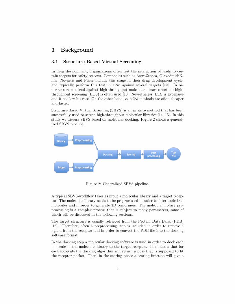
Structure-Based Virtual Screening (SBVS) is an in silico method that has beensuccessfully used to screen high-throughput molecular libraries [14, 15]. In thisstudy we discuss SBVS based on molecular docking. Figure 2 shows a general-ized SBVS pipeline.

Figure 2: Generalized SBVS pipeline.

A typical SBVS-workflow takes as input a molecular library and a target recep-tor. The molecular library needs to be preprocessed in order to filter undesiredmolecules and in order to generate 3D conformers. The molecular library pre-processing is a complex process that is subject to many parameters, some ofwhich will be discussed in the following sections.

The target structure is usually retrieved from the Protein Data Bank (PDB)[16]. Therefore, often a preprocessing step is included in order to remove aligand from the receptor and in order to convert the PDB-file into the dockingsoftware format.

In the docking step a molecular docking software is used in order to dock eachmolecule in the molecular library to the target receptor. This means that foreach molecule the docking algorithm will return a pose that is supposed to fitthe receptor pocket. Then, in the scoring phase a scoring function will give a

9

score to each pose. The higher the score the better the pose is supposed to fitthe target receptor. Finally, in the post-processing phase a group of best-scoringposes is selected and returned.

For high-throughput molecular libraries the whole process is compute-intensive.Therefore, in such case the molecular library needs to be partitioned and pro-cessed in parallel. However, the post-processing phase needs to take into accountthe whole dataset, therefore some distributed computing techniques need to beused.

3.2 Big Data analytics

Big Data analytics is a novel challenge in computer science. A fascinating studycarried out by Hilbert and Lopez [17] estimates how humankind data storagecapacity grew from 1986 to 2007.

Figure 3: Humankind storage capacity from 1986 to 2007. Retrieved from [17].

Figure 3 shows a linear growth, and digital storage overcoming analog storagein 2000s. According to Hilbert and Lopez in 2007 the humankind was able tostore 2.9 × 1020 optimally compressed bytes. While nowadays we are able tostore such a huge amount of data, we still have the problem of analyzing thatin reasonable time. Big Data analytics refers to a family of methods aimed toaddress that problem.

High-throughput methods in life science account for the growth of data size of

10

biological interest. For instance, Next-Generation Sequencing (NGS) machinescan sequence millions of reads in parallel, producing terabytes of raw data [18].Therefore, nowadays Big Data analytics is taking momentum in life science aswell. Also in SBVS, Big Data analytics applies, since we aim to screen high-throughput molecular libraries. In this study we showcased our tool with twowell-known libraries: eMolecules [2] and ZINC [1]. The free version of eMoleculescontains roughly 7 million molecules, while the whole ZINC database containsover 20 million molecules.

3.3 MapReduce

Google pioneered Big Data analytics with the Map Reduce (MR) programmingmodel, and were able to analyze twenty petabytes of data per day [6]. MRcomes with an implementation targeted to commodity computer clusters. Thismeans, as we discussed in the introduction, that MR application are out of thebox scalable, fault tolerant and cloud ready. In the MR-model, the programmerdescribe the computation with a Map and a Reduce function, and the MRframework takes care of implementation details such as locality-aware schedulingand data distribution.

The Map function takes a key/value pair in input and it returns a set of inter-mediate key/value pairs. In most MR-applications the input file contains singleline records, and the MR framework passes each line to the Map function, wherethe input key consists in the line number and the input value consists in theline content. Usually the programmer uses the Map-function in order to clusterthe input records.

The Reduce function takes a set of intermediate values with same key andreturns a final key/value pair. In the Reduce facet, the programmer usuallydiscerns something useful from each cluster generated in the Map functions. Anexample will make this more clear to the reader.

3.3.1 Consensus problem in MapReduce

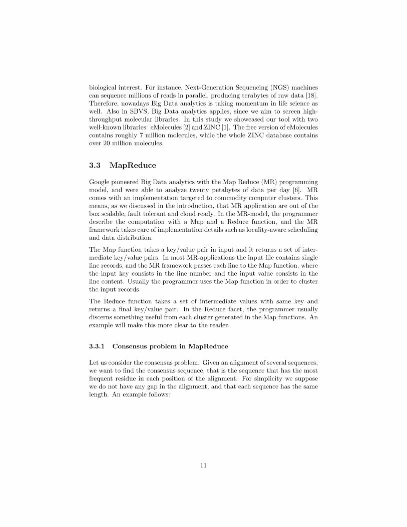
Let us consider the consensus problem. Given an alignment of several sequences,we want to find the consensus sequence, that is the sequence that has the mostfrequent residue in each position of the alignment. For simplicity we supposewe do not have any gap in the alignment, and that each sequence has the samelength. An example follows:

11

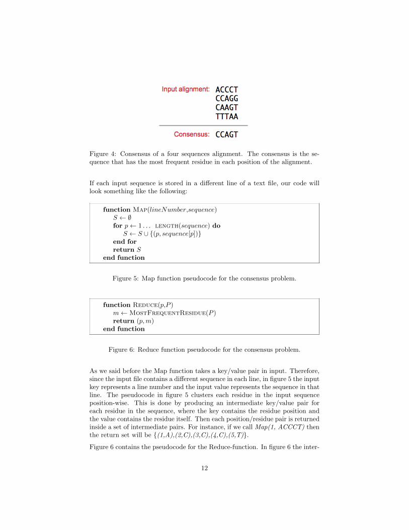
Figure 4: Consensus of a four sequences alignment. The consensus is the se-quence that has the most frequent residue in each position of the alignment.

If each input sequence is stored in a different line of a text file, our code willlook something like the following:

function Map(lineNumber,sequence)S ← ∅for p← 1 . . . length(sequence) do

S ← S ∪ {(p, sequence[p])}end forreturn S

end function

Figure 5: Map function pseudocode for the consensus problem.

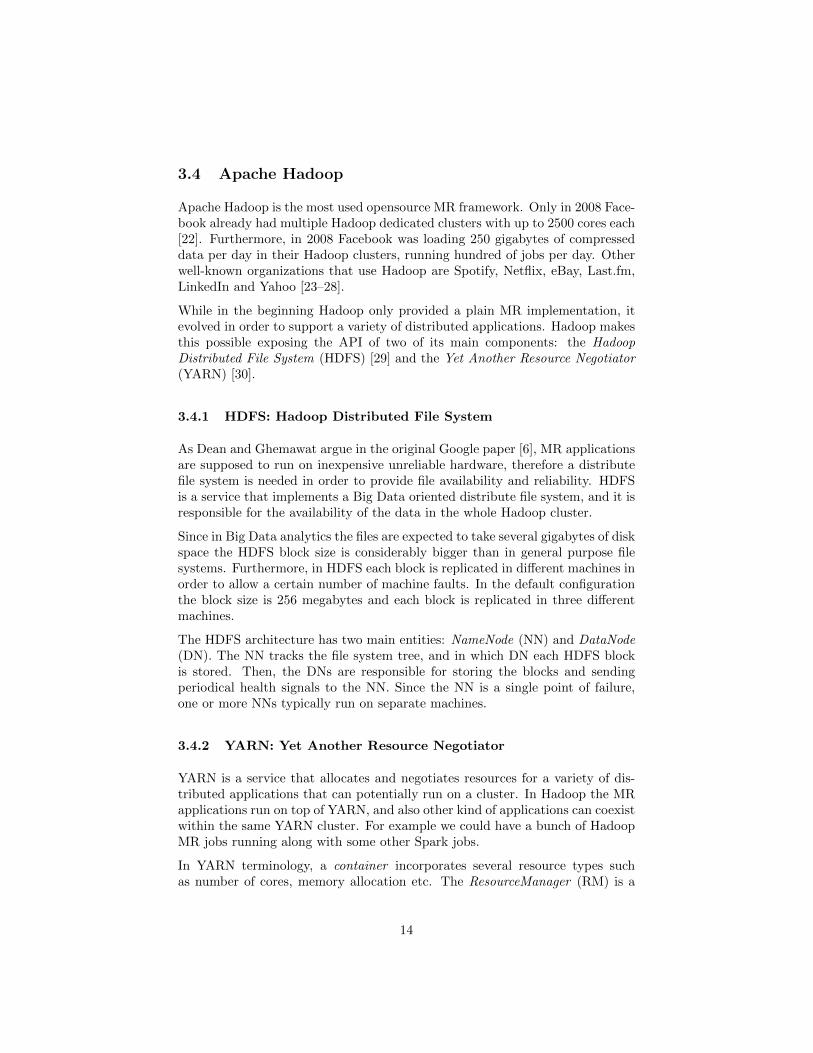
function Reduce(p,P )m←MostFrequentResidue(P )return (p,m)

end function

Figure 6: Reduce function pseudocode for the consensus problem.

As we said before the Map function takes a key/value pair in input. Therefore,since the input file contains a different sequence in each line, in figure 5 the inputkey represents a line number and the input value represents the sequence in thatline. The pseudocode in figure 5 clusters each residue in the input sequenceposition-wise. This is done by producing an intermediate key/value pair foreach residue in the sequence, where the key contains the residue position andthe value contains the residue itself. Then each position/residue pair is returnedinside a set of intermediate pairs. For instance, if we call Map(1, ACCCT) thenthe return set will be {(1,A),(2,C),(3,C),(4,C),(5,T)}.

Figure 6 contains the pseudocode for the Reduce-function. In figure 6 the inter-

12

mediate key p is a position number, and the set of intermediate values P containssome residues at that position. If the Reduce-code is defined in order to be com-mutative and associative, we can assume that P contains all of the residues atposition p. Therefore, in figure 6 the most frequent residue m is extracted, and afinal key/value pair (p,m) is returned. For example Map(1, {A,C,C,T}) returns(1, C). Finally, the MR-framework is responsable for collecting all of the finalkey/value pairs and producing the consensus sequence.

3.3.2 MR open source ecosystem

In this section we want to give a brief overview of the frameworks available inthe opensource MR ecosystem, other than Spark.

Apache Hadoop is with no doubt the most used open source MR implementa-tion. In recent versions Hadoop can run many type of distributed applicationsother than MR, and it supports dataset caching for sequential MR operations.Many distributed frameworks such as Apache Pig [9], Apache Hive [19], ApacheFlink [20] and even Spark [10] take advantage of this. Pig and Hive providea layer of abstraction on top of Hadoop. Pig is script oriented, and thereforemore appealing to scripting developers, while Hive is database oriented andmore appealing to SQL developers. Flink is a young project that is somewhatcomparable to Spark, and it has a sophisticate support for pipelining.

Another notable tool in the MR ecosystem is Spotify Luigi [8]. Luigi offers alevel of abstraction that allows the user to pipe dataset transformations writtenusing different frameworks (such as Hadoop and Spark). In addition, Luigican schedule independent jobs on different machines, and it has a nice UserInterface (UI) to monitor the overall pipeline status. Finally, MongoDB [21] isa document oriented Database Management System (DBMS) that has built-insupport to MR transformations.

3.3.3 MR limitations

Even though Google’s MR pioneered Big Data analytics, it has some limitationsthat make it not suitable for certain problems. First it has a strict life cycle.In fact, in MR a Map dataset transformation have to be followed by a Reducetransformation. Furthermore, the MR specification does not say anything aboutshared variables such as broadcast variables or accumulators. Also, third partysoftwares for pipelining need to be used, and there is no caching of the datasetfor iterative jobs. Finally, in MR there is poor support for global sorting.

13

3.4 Apache Hadoop

Apache Hadoop is the most used opensource MR framework. Only in 2008 Face-book already had multiple Hadoop dedicated clusters with up to 2500 cores each[22]. Furthermore, in 2008 Facebook was loading 250 gigabytes of compresseddata per day in their Hadoop clusters, running hundred of jobs per day. Otherwell-known organizations that use Hadoop are Spotify, Netflix, eBay, Last.fm,LinkedIn and Yahoo [23–28].

While in the beginning Hadoop only provided a plain MR implementation, itevolved in order to support a variety of distributed applications. Hadoop makesthis possible exposing the API of two of its main components: the HadoopDistributed File System (HDFS) [29] and the Yet Another Resource Negotiator(YARN) [30].

3.4.1 HDFS: Hadoop Distributed File System

As Dean and Ghemawat argue in the original Google paper [6], MR applicationsare supposed to run on inexpensive unreliable hardware, therefore a distributefile system is needed in order to provide file availability and reliability. HDFSis a service that implements a Big Data oriented distribute file system, and it isresponsible for the availability of the data in the whole Hadoop cluster.

Since in Big Data analytics the files are expected to take several gigabytes of diskspace the HDFS block size is considerably bigger than in general purpose filesystems. Furthermore, in HDFS each block is replicated in different machines inorder to allow a certain number of machine faults. In the default configurationthe block size is 256 megabytes and each block is replicated in three differentmachines.

The HDFS architecture has two main entities: NameNode (NN) and DataNode(DN). The NN tracks the file system tree, and in which DN each HDFS blockis stored. Then, the DNs are responsible for storing the blocks and sendingperiodical health signals to the NN. Since the NN is a single point of failure,one or more NNs typically run on separate machines.

3.4.2 YARN: Yet Another Resource Negotiator

YARN is a service that allocates and negotiates resources for a variety of dis-tributed applications that can potentially run on a cluster. In Hadoop the MRapplications run on top of YARN, and also other kind of applications can coexistwithin the same YARN cluster. For example we could have a bunch of HadoopMR jobs running along with some other Spark jobs.

In YARN terminology, a container incorporates several resource types suchas number of cores, memory allocation etc. The ResourceManager (RM) is a

14

component that accepts application submissions and negotiates containers forthe whole cluster. When an application is submitted the RM is responsible fornegotiating the ApplicationMaster (AM) container, and for restarting it in caseof failure. In many setups, one or more RMs run on dedicated machines alongwith HDFS NNs.

The AM is a per-application service that negotiates/restarts containers with theRM for its own application. Furthermore, the AM attempts to get containerswhere the data relevant to the application is stored, minimizing the networkcommunication.

Finally, on each compute node in the cluster runs a service called NodeManager(NM). The NM manages the containers within its node, and it reports theiravailability and health status to the RM.

3.5 Spark

Spark is a cluster computing framework that aims to overcome the limitations ofMR while still providing scalability, fault tolerance and cloud runnability. As wediscussed before, MR penalizes performance in applications where a working setundergoes successive transformations. Improving the performance for this classof problems was the aim of the original Spark implementation [10]. To achievethis goal Spark introduces a dataset abstraction called Resilient DistributedDataset (RDD) [31].

Even if it can run stand-alone, Spark gives the possibility to access HDFS andYARN services. From our experience, running Spark jobs on top of HDFS andYARN is more flexible and user-friendly.

3.5.1 RDD: Resilient Distributed Dataset

An RDD is a read-only collection of records partitioned through the nodes inthe cluster. It can be created either from stored data (e.g. HDFS), or through atransformation of a previously created RDD. While in MR only map and reducetransformations are allowed, Spark offers a broader set of transforms that canbe applied in any order. Some transformations that are offered to the userout of the box, apart form map and reduce, are: sortBy, groupBy, filter, unionand intersection. For a more detailed RDD transformations list please refer toZaharia et al. [31].

Spark exposes RDDs through a Scala, Java [32] or Python [33] API. Therefore,the user can pick its favorite programming language among the previous, inorder to define one or more RDDs. However, from our experience we noticedthat the Scala API is better maintained and it leads to better performance.This is not surprising since Spark is implemented in Scala.

15

Apart from transformations, the user can apply actions to RDDs that eitherreturn a value, or save the data in the file system. In addition, a cache methodcan be called on RDDs in order to cache the data for future transformations.This is the key feature that allows the performance improvement in successiveworking set transformations. Finally, Spark computes RDDs lazily in order topipeline transformations, and each RDD maintains enough information on howit was derived, so that in case of fault a lost partition can be recomputed.

3.5.2 Shared variables

Along with RDDs the Spark API offers to the user the possibility to define twotypes of shared variables: broadcast variables and accumulators.

Broadcast variables are read-only objects that are shipped to each node. Theycan be used in order to efficiently ship a large object that is needed in eachnode.

Accumulators are variables that can be updated only through an associativeoperation, and that become readable at the end of the computation. They areoften used in order to implement counters or sums.

Comparing with MR, shared variables make Spark suitable for a broader rangeof problems.

3.5.3 Consensus problem in Spark

In the following we solve the consensus problem in Spark under the same as-sumptions we used in the MapReduce section. We choose to use the Scala APIfor this example.

1 //Spark context initialization

2 val conf = new SparkConf()

3 .setAppName("Consensus example")

4 .setMaster("yarn-cluster")

5 val sc = new SparkContext(conf)

6 //Compute consensus

7 val rdd = sc.textFile("hdfs://path/to/sequences.txt") //read the input

8 val consensus = rdd

9 .flatMap(seq => seq.zipWithIndex.map(_.swap)) //first transformation

10 .groupByKey //second transformation

11 .map((p,P) => mostFrequentResidue(P)) //third transformation

12 .collect //action

13 println(consensus.mkString) //print the result

Figure 7: Spark code for the consensus problem.

16

In Figure 7 we fist initialize Spark. The SparkConf object is used in orderto specify an application name, and the spark master. The Spark master is aparameter that specifies if the application will be run in stand-alone mode orusing YARN. In figure 7 we set the spark master in order to run in YARN mode(line 4).

The first RDD is created reading the input sequences file from HDFS (line7), and a cascade of transformations is then applied in order to compute theconsensus sequence. The first transformation uses some “syntactic sugar” inorder to emit the intermediate key/value pairs, like we have done in figure 5.Since in Spark the map transformation does not allow to emit multiple key/valuepairs we use a flatMap instead. Then the lambda expressions we pass to theflatMap, zips each residue in the input sequence with its position (or index),producing a residue/position pair. Then, since we want the position to be thekey in the intermediate pairs, we swap residue and position.

The second transformation groups the intermediate key/values pairs by key.Since we set the residue position to be the key, Spark will cluster all of theresidues at the same position together.

The third transformation maps each group produced in the previous one tothe most frequent residues in it. The lambda expression passed to the maptransform its equivalent to the pseudocode in figure 6.

Finally, an action it is applied to the last RDD in order to collect the most fre-quent residue at each position (line 12), and the consensus is printed out.

3.5.4 Spark SQL and Spark MLlib

In this section we give a short overview of two interesting projects that are dis-tributed along with Spark. These projects enrich the Spark API and implementmany useful algorithms for big data analytics.

Spark SQL [34] introduces a level of abstraction for working with structureddata. It supports input data structured in different flavours e.g. Apache Hive,Parquet [35] files, JSON [36] files, as well as standard JDBC/ODBC [37, 38]database connections. Spark SQL’s main feature is to allow SQL [39] queriesover RDDs.

Spark MLlib [40] is a machine learning library. It defines a labelled point RDDtype that can be used in order to train a model with different kind of algorithms.Labeled point RDDs can be created from LIBSVM [41] files, from custom fileformats, and through RDD transformations. Spark MLlib offers supervised andunsupervised learning, and includes well-known algorithms such as Lasso [42],Ridge [43], SVM [44], random forest [45] and k-means [46].

17

3.5.5 Why Spark for SBVS

In this paper we discuss the applicability of big data analytic techniques inSBVS. Therefore, we first investigated which of the MR frameworks in the MRopen source ecosystem best fits the SBVS pipelines. Hadoop and Spark areboth mature projects, and have been successfully used by various organizations.However, even if it is possible to implement SBVS in Hadoop [47], the plain MR-model in it hardly fits the problem. First, in Hadoop each map transformationneeds to be followed by a reduce one. In the SBVS pipelines datasets do notneed to be reduced until the post-processing phase is reached. It is true thateach of the steps before the post-processing phase could be merged in a big maptransformation, but this would lead to poor testability and configurability. InSpark there is not such problem since the RDD transformations can be definedin any order.

In addition, there is no support for pipelines in Hadoop. This would make itmandatory to use third party products in order to define pipelines. In contrast,Spark RDDs are processed lazily, making it easy to pipeline transformationsusing Scala, Java or Python syntax.

Hadoop API does not either offer broadcast variables. This makes it tricky tosend the target receptor to each node in the docking phase. Sure, it wouldbe possible to pack the receptor in the map code as a binary array, or evenmanually copy the receptor in each node. However, this would be inefficientand in more in general tedious. Spark API offers broadcast variables that aremeant to efficiently send read-only data to each node, and therefore it gracefullysolves the problem.

Finally, the sortBy transformations in Spark, allows to sort poses by score easilyif we compare to the shuffle and sort phase in Hadoop.

To summarize, we chose Spark for SBVS because it allows configuration of theorder of the dataset transformations, it gives built-in support for pipelines, it hasbroadcast variables, and because it offers a simple way to sort the dataset.

3.6 Cheminformatics

Cheminformatics is a family of in silico methods aimed to aid the process of drugdevelopment [48]. Those include chemical representations, chemical libraries,and tools for chemical processing. In this section we give an overview of thecheminformatics methods we used in this study.

3.6.1 Molecular representations: SMILES and SDF

SMILES and SDF are two chemical structure representation formats [49, 50].While SMILES is lightweight-oriented and can be used in order to represent

18

stereochemistry and atom connections in a molecule, SDF is a considerablyheavier format and provides a way to represent atom coordinates as well. Sincewhen using the SMILES format, a molecule can be represented with a singlerelatively short string, SMILES molecules can be quickly written down by anexperienced user. However, many applications require the 3D-representationprovided by the SDF format. Hence, a typical case is to first represent a moleculeusing the SMILES format and then to go through a preprocessing phase inorder to generate the relative SDF representation. Nevertheless, SMILES canbe stereochemically ambiguous, and even if they specify stereochemistry, morethan one low energy conformer can correspond to a stereoisomer. Therefore,this preprocessing phase typically produces more than one SDF representationfor a SMILES molecule.

3.6.2 Molecular libraries: ZINC and eMolecules

ZINC and eMolecules are two molecular libraries suitable for high-throughputvirtual screening [1, 2].

ZINC is freely accessible and contains over 20 million commercially availablemolecules. Each molecule in ZINC is in ready-to-dock format, and can bedownloaded in SDF-format. For this reason, ZINC-subsets can be used in SBVSskipping the preprocessing phase.

In contrast, eMolecule is a legacy molecular library and can be fully accessedonly after subscription. However, a free version of the database containigroughly 7 million molecules can be downloaded for free in SMILES and 2D SDFformat. Since those formats do not provide a 3D-representation, a preprocessingstep is required in SBVS.

Both ZINC and eMolecules, along with the library, give a rather sophisticateweb-application that allows to search and purchase molecules.

3.6.3 OpenEye toolkits

The OpenEye toolkits are a set of cheminformatics and modelling programminglibraries [51]. Since they expose a Java API, they are suitable to work withSpark. In this study we mainly used three of the tools included in the OpenEyetoolkits package: MolProp, Omega and OEDocking.

MolProp is a tool for molecular property calculation and filtering. In SBVSfiltering is a crucial step in the molecular library preprocessing phase. In fact,we do not want to dock a target receptor to molecules that do not look likeleads. For this purpose, MolProp offers some default filter types as well as thepossibility to define a custom type. Among the ready to use filter types, thelead-like filter is particularly interesting for our case. In addition, the Mol-

19

Prop filter includes a preprocessing step that removes salts and metals from themolecules.

Omega is a molecular 3D conformer generator. As we explained before, molecu-lar libraries that do not provide 3D information need to be preprocessed in orderto be docked to a receptor. Therefore, this is a step that might be included inthe SBVS preprocessing phase of some molecular libraries. Since several con-formers may correspond to a 2D representation within Omega, two parameterscan be specified in order to control how may of them will be produced. First,we can set the number of stereocenters to be considered for stereochemicallyambiguous molecules. This means that if we decide to consider N stereocenters2N stereoisomers will be generated. Then, for each of the stereoisomers previ-ously produced we can decide the maximum number of low energy conformersto return.

OEDocking is a tool for molecular docking. It requires molecular 3D represen-tation for the ligands, and it can read them from a SDF-file. In contrast, thetarget receptor must be represented in the OpenEye legacy format. However,this is not a big deal since OEDocking provides a handy tool that can create atarget receptor file from a PDB entry. In addition, since PDB entries are oftenprovided with a ligand, the pocket can be recognized automatically. OEDockingimplements an exhaustive search algorithm in which the ligand is rotated insidethe pocket with a certain resolution. Then, each of the resulting poses is scoredwith a user specified scoring function, and only the one with highest score isreturned.

20

4 Implementation

In this project we used Spark in order to parallelize the code. Even if, Spark-based applications are relatively simple to implement, some solutions that weused are not trivial and are discussed in this section. First, we discuss theprogramming model that we developed in order to make pipeline definitioneasier. Then, we give some implementation details.

4.1 Programming model

In order to provide better configurability we implemented a scala library that canbe user in order to define ad-hoc SBVS pipelines. SBVSPipeline is the core classin our tool. When the user creates a new SBVSPipeline object, he/she specifiesa Spark context, and we say that the pipeline is in the Init state. Then, eachtime the user calls a method from the SBVSPipeline object, a transformation inthe underling RDD occurs, and there might be a state transition. The graph infigure 8 shows states and transitions a SBVSPipeline object can undergo.

Figure 8: SBVSPipeline object states and transitions graph.

Within the Init state the user can call three methods: readSmilesFile, readCon-formerFile and readPoseFile. These read a user specified text file and changesthe state respectively into SMILES, Conformer or Pose. The user is supposedto specify a SMILES-file if he/she uses the readSmilesFile, and otherwise a SDFfile. In addition, readConformerFile should be used to read conformers, andreadPoseFile should be used to read scored poses. Since the files in SBVS arebig there is no control for the correctness of the provided file.

21

The SMILES state has two main methods. The first one is filter, and it can beused in order to filter out undesired molecules from the dataset. We supportOpenEye’s default and custom filters. The other method that can be usedwithin the SMILES status is generateConformers. It takes two paramentersthat specify how many stereocenters to consider for stereochemically ambiguousmolecules, and the maximum number of low energy comformers to return foreach stereoisomer. This method causes a transition into the Pose status.

The dock method can be used within the Conformer status. It docks each ofthe conformers in the underling RDD to a user specified target receptor. Inaddition, the user specifies the ligand rotation resolution and a scoring functionto use. The dock method causes a transition into the Pose state.

Two main methods can be used within the Pose state. The sortByScore methodsorts all of the molecules in the underling RDD by score. In addition, sinceduring the conformer generation many conformers can be generated from asingle SMILES molecule, the collapse method can be used in order to reducethe poses relative to a single SMILES molecule to N best scoring poses. Noneof the methods that can be called within the Pose state cause transition.

Finally, the saveAsTextFile method can be called within SMILES, Conformeror Pose states in order to save the underling RDD into the storage system. Itdoes not cause any state transition.

4.2 Implementation details

The filter, the generateConformers and the dock methods are implemented usingOpenEye toolkits.

OEDocking requires the receptor file to be in its legacy format, and does notprovide a method to read it from HDFS. Therefore, we read the receptor oncefrom the general purpose file system and then we use a Spark broadcast variablein order to make it available in each node.

We implemented two custom Hadoop record readers in order to allow our appli-cation to read SDF and SMILES molecules from HDFS. Since OpenEye objectsrequire a considerable amount of memory we need to reuse them as much aspossible. For this reason a record size parameter in our custom record read-ers can be set in order to decide how many molecules will be read and storedin a single record. The higher the record size is, the more the OpenEye ob-jects will be reused. However, too high setting of record size could lead to loadimbalances.

The saveAsTextFile and sortByScore method were implemented with Sparkbuilt-in RDD transformations. Also the collapse method it is easy to implementin Spark. In fact, it consists in a “group by id” transformation followed by a“reduce by best score” one.

22

5 Examples

In figure 1 we already gave an example of SBVSPipeline usage. The aim of thissection is to give a couple of additional examples for real world cases.

5.1 Standardization pipeline

As we discussed before, molecular libraries usually need to undergo a preprocess-ing phase in order to be ready for docking. This process can be computationallyheavy, but once it is done there is no need to repeat it. For this reason organiza-tions that maintain their own high-throughput molecular libraries usually havea standardization pipeline aimed to preprocess new molecules before insertion.Needless to say, the standardization pipeline definition depends on the molecularlibrary purpose. A simple standardization pipeline defined using SBVSPipelinefollows.

1 new SBVSPipeline(sc)

2 .readSmilesFile("hdfs://path/to/new-molecules.smi")

3 .filter("/path/to/filter-rules.txt")

4 .generateConformers(0,1) //0 stereocenters, max 1 conformer

5 .saveAsTextFile("hdfs://path/to/standardized.sdf")

Figure 9: Simple standardization pipeline.

In figure 9 we start by reading an input SMILES file from HDFS. Then, we filterthe dataset using some custom filter rules defined in a filter-rules.txt file. Finally,we generate and save the 3D-conformers in SDF-format. Please notice that atline 4 we specified maximum one low energy conformer per stereoisomer, and weassumed that every SMILES molecule in the input file specifies stereochemistry.The last one is generally a too strong assumption. Furthermore, it is goodpractice to have some primary custom filtering rules to apply to every dataset,and then use the default OEDocking filters as a refinement for more specificcases.

1 new SBVSPipeline(sc)

2 .readSmilesFile(hdfs://path/to/new-molecules.smi")

3 .filter("/path/to/primary-rules.txt")

4 .filter(OEFilterType.Lead)

5 .repartition

6 .generateConformers(2,1) //2 stereocenters, max 1 conformer

7 .saveAsTextFile("hdfs://path/to/standardized.sdf")

Figure 10: “Ready-to-dock” standardization pipeline.

23

In figure 10 we defined a standardization pipeline that generates ready-to-dockmolecules from an input SMILES file in which some molecules might not specifystereochemistry. Here we set the maximum number of considered stereocentersfor stereochemically ambiguous molecules to 2, like suggested by Irwin et al. [1].Furthermore, we apply a primary general rules filter and then we further refinethe dataset applying the OpenEye’s lead-like default filter.

5.2 Screening pipeline

Let us suppose we have a ready-to-dock molecular library, that we either stan-dardized ourselves or we retrieved from a provider such as ZINC. A typical usecase is to screen this molecular library against a target receptor. A pipeline forsuch purpose can be defined using the SBVSPipeline as follows.

1 val res = new SBVSPipeline(sc)

2 .readConformerFile("hdfs://path/to/conformers.sdf")

3 .dock("/path/to/receptor.oeb", OEDockMethod.Chemgauss4,

4 OESearchResolution.Standard)

5 .collapse(3) //keep only 3 best scoring pose with same ID

6 .sortByScore

7 .getMolecules

8 .take(30) //take first 30

Figure 11: Screening pipeline.

In figure 11 we start by reading an SDF conformers file from HDFS. Then weproceed with the docking phase, using Chemgauss4 [52] scoring function andStandard rotation resolution. An important assumption that we make is thatin the standardization phase we set an identifier in order to recognize conformersthat were derived from the same SMILES molecule. Hence, the collapse methodis able to reduce the poses with the same identifier to only 3 best scoring poses.Finally, we sort the molecules by score and we take the top 30 hits.

Since the docking phase usually takes a lot of time, is important to checkpointthe computation after the docking phase. This consists in saving the poses backto HDFS before proceeding. This allows to postprocess the poses in a differentway later without repeating the docking phase. Line 5 in figure 12 shows howto checkpoint.

24

1 val res = new SBVSPipeline(sc)

2 .readConformerFile("hdfs://path/to/conformers.sdf")

3 .dock("/path/to/receptor.oeb", OEDockMethod.Chemgauss4,

4 OESearchResolution.Standard)

5 .saveAsTextFile("/path/to/checkpoint-poses.sdf")

6 .collapse(3) //keep only 3 best scoring pose with same ID

7 .sortByScore

8 .getMolecules

9 .take(30) //take first 30

Figure 12: Screening pipeline with checkpoint.

25

6 Materials and methods

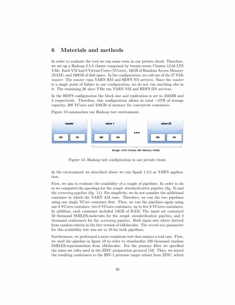
In order to evaluate the tool we run some tests in our private cloud. Therefore,we set up a Hadoop 2.5.2 cluster composed by twenty-seven Ubuntu 12.04 LTSVMs. Each VM had 8 Virtual Cores (VCores), 16GB of Random Access Memory(RAM), and 160GB of disk space. In the configuration, we call one of the 27 VMsmaster. The master runs YARN RM and HDFS NN services. Since the masteris a single point of failure in our configuration, we do not run anything else init. The remaining 26 slave VMs run YARN NM and HDFS DN services.

In the HDFS configuration the block size and replication is set to 256MB and3 respectively. Therefore, this configuration allows in total ∼4TB of storagecapacity, 208 VCores and 416GB of memory for concurrent containers.

Figure 13 summarizes our Hadoop test environment.

Figure 13: Hadoop test configuration in our private cloud.

In the environment we described above we run Spark 1.2.2 as YARN applica-tion.

First, we aim to evaluate the scalability of a couple of pipelines. In order to doso we computed the speedups for the simple standardization pipeline (fig. 9) andthe screening pipeline (fig. 11). For simplicity, we do not consider the additionalcontainer in which the YARN AM runs. Therefore, we run the two pipelinesusing one single VCore container first. Then, we run the pipelines again usingone 8 VCores container, two 8 VCores containers, up to five 8 VCores containers.In addition, each container included 14GB of RAM. The input set contained50 thousand SMILES-molecules for the simple standardization pipeline, and 2thousand conformers for the screening pipeline. Both input sets where derivedfrom random entries in the free version of eMolecules. The record size parameterfor this scalability test was set to 10 for both pipelines.

Furthermore, we performed a more consistent test that mimics a real case. First,we used the pipeline in figure 10 in order to standardize 100 thousand randomSMILES-representation from eMolecules. For the primary filter we specifiedthe same set rules used in the ZINC preparation protocol [53]. Then, we mixedthe resulting conformers to the HIV-1 protease target subset from ZINC, which

26

counts 60 conformers. Then, our aim was to use the pipeline in figure 12 inorder to find HIV-1 protease hits in the mixed dataset. For this purpose, wegenerated the HIV-1 protease receptor file from the 1AJV PDB entry [54] usingthe OpenEye’s command line tool. This more consistent test was run usingtwenty-five 7 VCores containers with 14GB of RAM, plus an additional singlecore container for the YARN AM. For this test record size was set to 80 for thestandardization part and to 30 for the screening part.

27

7 Results

Running time tables and speedup plots for the scalability test follow.

Simple standardization pipelineVCores Running time

1 3h 55’ 28”8 50’ 01”16 27’ 56”24 19’ 43”32 15’ 47”40 13’ 43”

Table 1: Running time table for the simple standardization pipeline (fig. 9)scalability test. Every row corresponds to a run over a 50 thousand SMILES-molecules input.

Screening pipelineVCores Running time

1 4h 15’ 32”8 1h 12’ 59”16 38’ 25”24 29’ 03”32 20’ 07”40 17’ 54”

Table 2: Running time table for the screening pipeline (fig. 11) scalability test.Every row corresponds to a run over a 2 thousand SDF-conformers input.

28

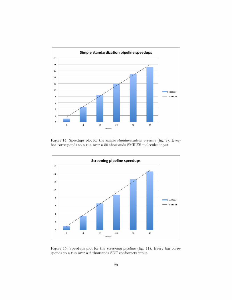
Figure 14: Speedups plot for the simple standardization pipeline (fig. 9). Everybar corresponds to a run over a 50 thousands SMILES molecules input.

Figure 15: Speedups plot for the screening pipeline (fig. 11). Every bar corre-sponds to a run over a 2 thousands SDF conformers input.

29

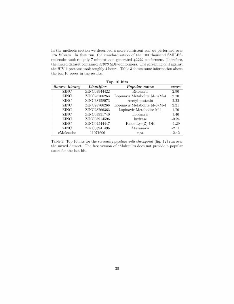
In the methods section we described a more consistent run we performed over175 VCores. In that run, the standardization of the 100 thousand SMILES-molecules took roughly 7 minutes and generated 40960 conformers. Therefore,the mixed dataset contained 41020 SDF-conformers. The screening of if againstthe HIV-1 protease took roughly 4 hours. Table 3 shows some information aboutthe top 10 poses in the results.

Top 10 hitsSource library Identifier Popular name score

ZINC ZINC03944422 Ritonavir 2.90ZINC ZINC28766263 Lopinavir Metabolite M-3/M-4 2.70ZINC ZINC38158973 Acetyl-pestatin 2.22ZINC ZINC28766266 Lopinavir Metabolite M-3/M-4 2.21ZINC ZINC28766363 Lopinavir Metabolite M-1 1.70ZINC ZINC03951740 Lopinavir 1.40ZINC ZINC03914596 Invirase -0.24ZINC ZINC04544447 Fmoc-Lys(Z)-OH -1.29ZINC ZINC03941496 Atazanavir -2.11

eMolecules 11071606 n/a -2.42

Table 3: Top 10 hits for the screening pipeline with checkpoint (fig. 12) run overthe mixed dataset. The free version of eMolecules does not provide a popularname for the last hit.

30

8 Discussion and conclusion

The simple standardization pipeline (fig. 9) and the screening pipeline (fig. 11)count 5 and 8 lines of code respectively, and can be written in a few minutesby an experienced user. Therefore, the first advantage of our tool is productiv-ity.

The results in table 2 and table 1 show how adding VCores the running timedecreases considerably. In addition, the speedup plots in figure 14 and in figure15 show a linear growth. This means that the two pipelines scale well. However,the speedup that we observe in the 40 core run is ∼17 in figure 14 and ∼15 infigure 15. In contrast, we would expect a speedup that approaches 40, thatis the level of parallelism. This happens because some load imbalance occurs.We believe that the load imbalance can be attenuated tuning the record sizeparameter. Nevertheless, in molecular libraries some molecules are bigger thanothers and therefore the dataset splits will take different time to be processed.However, this is a problem that occurs also in MPI implementations.

The more consistent run shows how, with adequate cloud resources, real worldcases can be run over night. Most of the molecules in table 3 are not surprisinglyHIV-1 protease inhibitors from the ZINC subset. The eMolecules hit might bea lead HIV-1 protease drug, but since the free version of eMolecules does notprovide enough information we cannot be sure.

The results shows that when using our tool a user can easily set up scalablemassively parallel SBVS pipelines. However, many improvements in the tool,such as better load balancing, can be done.

In this study we have shown that Spark applies to SBVS, and it is in generala suitable solution for massively parallel pipelining. In addition, we point outthat Big Data analytics is beneficial in life science datasets as well.

Finally, we want to emphasize that all our test were run in a cloud environ-ment, and this open-ups SBVS to these organizations that do not own HPCfacilities.

31

References

[1] Irwin JJ, Sterling T, Mysinger MM, Bolstad ES, and Coleman RG. ZINC:a free tool to discover chemistry for biology. J Chem Inf Model, 52(7):1757–1768, Jul 2012.

[2] eMolecules database (free version). Last update 2015-04-01. eMoleculesInc., La Jolla, CA, USA. http://www.emolecules.com.

[3] Norgan AP, Coffman PK, Kocher JP, Katzmann DJ, and Sosa CP. Multi-level Parallelization of AutoDock 4.2. J Cheminform, 3(1):12, 2011.

[4] OEDocking. Version 3.0.1. OpenEye Scientific Software, Santa Fe, NM,USA. http://www.eyesopen.com.

[5] Message Passing Interface Forum. MPI: A Message-Passing Interface Stan-dard. International Journal of Supercomputing Applications, 8(3/4):165–414, 1994.

[6] Dean J and Ghemawat S. Mapreduce: Simplified data processing on largeclusters. Commun. ACM, 51(1):107–113, January 2008.

[7] Apache Hadoop. Version 2.6.0. The Apache Software Fundation, ForestHill, MD, USA. http://hadoop.apache.org.

[8] Spotify Luigi. Commit 07efdd9. Spotify AB, Stockholm, Sweden. https:

//github.com/spotify/luigi.

[9] Apache Pig. Version 0.14.0. The Apache Software Fundation, Forest Hill,MD, USA. http://pig.apache.org.

[10] Zaharia M, Chowdhury M, Franklin MJ, Shenker S, and Stoica I. Spark:Cluster computing with working sets. In Proceedings of the 2Nd USENIXConference on Hot Topics in Cloud Computing, HotCloud’10, pages 10–10,Berkeley, CA, USA, 2010. USENIX Association.

[11] Scala programming language. Version 2.11.5. Polytechnique FA c©dA c©ralede Lausanne, Lausanne, Switzerland. http://www.scala-lang.org.

[12] Bowes J, Brown AJ, Hamon J, Jarolimek W, Sridhar A, Waldron G, andWhitebread S. Reducing safety-related drug attrition: the use of in vitropharmacological profiling. Nat Rev Drug Discov, 11(12):909–922, December2012.

[13] Cheng T, Li Q, Zhou Z, Wang Y, and Bryant SH. Structure-based virtualscreening for drug discovery: a problem-centric review. The AAPS Journal,14(1):133–141, Mar 2012.

[14] Seifert MH and Lang M. Essential factors for successful virtual screening.Mini Rev Med Chem, 8(1):63–72, Jan 2008.

32

[15] Villoutreix BO, Eudes R, and Miteva MA. Structure-based virtual ligandscreening: recent success stories. Comb. Chem. High Throughput Screen.,12(10):1000–1016, Dec 2009.

[16] Berman HM, Westbrook J, Feng Z, Gilliland G, Bhat TN, Weissig N,Shindyalov IN, and Bourne PE. The protein data bank. Nucleic AcidsRes, 28:235–242, 2000.

[17] Hilbert M and Lopez P. The world’s technological capacity to store, com-municate, and compute information. Science, 332(6025):60–65, Apr 2011.

[18] Wandelt S, RheinlAnder A, Bux M, Thalheim L, Haldemann B, and LeserU. Data management challenges in next generation sequencing. Datenbank-Spektrum, 12(3):161–171, 2012.

[19] Apache Hive. Version 1.1.0. The Apache Software Fundation, Forest Hill,MD, USA. http://hive.apache.org.

[20] Apache Flink. Version 0.9.0. The Apache Software Fundation, Forest Hill,MD, USA. http://flink.apache.org.

[21] MongoDB. Version 3.0. MongoDB Inc., Dublin, Ireland. http://www.

mongodb.org/.

[22] Sarma JS. Hadoop. http://web.archive.org/web/20080207010024/

http://www.808multimedia.com/winnt/kernel.htm, Jun 2008. Date vis-ited 15 Apr 2015.

[23] Whiting D. Data Processing with Apache Crunch at Spotify. https:

//labs.spotify.com/2014/11/27/crunch/, Nov 2014. Date visited 15Apr 2015.

[24] Krishnan S and Tse E. Hadoop Platform as a Servicein the Cloud. http://techblog.netflix.com/2013/01/

hadoop-platform-as-service-in-cloud.html, Jan 2013. Date visited15 Apr 2015.

[25] Madan A. Hadoop - The Power of the Elephant. http://www.

ebaytechblog.com/2010/10/29/hadoop-the-power-of-the-elephant/

#.VS5DHZSUeos, Oct 2010. Date visited 15 Apr 2015.

[26] Bosteels K. Python + Hadoop = Flying Circus Elephant. http://blog.

last.fm/2008/05/29/python-hadoop-flying-circus-elephant, May2008. Date visited 15 Apr 2015.

[27] Hayes M. White Elephant: The Hadoop Tool You Never KnewYou Needed. https://engineering.linkedin.com/hadoop/

white-elephant-hadoop-tool-you-never-knew-you-needed, Mar2013. Date visited 15 Apr 2015.

[28] Liu F and Singh S. White Elephant: The Hadoop Tool You NeverKnew You Needed. https://engineering.linkedin.com/hadoop/

33

white-elephant-hadoop-tool-you-never-knew-you-needed, Mar2013. Date visited 15 Apr 2015.

[29] Vavilapalli VK, Murthy AC, Douglas C, Agarwal S, Konar M, Evans R,Graves T, Lowe J, Shah H, Seth S, Saha B, Curino C, O’Malle O, RadiaS, Reed B, and Baldeschwieler E. Apache hadoop yarn: Yet another re-source negotiator. In Proceedings of the 4th Annual Symposium on CloudComputing, pages 5:1–5:16, New York, NY, USA, 2013. ACM.

[30] Rixner S Shafer J and Cox AL. The hadoop distributed filesystem: Bal-ancing portability and performance. In IEEE International Symposium onPerformance Analysis of Systems and Software, pages 122 – 133, WhitePlains, NY, USA, Mar 2010. IEEE.

[31] Zaharia M, Chowdhury M, Das T, Dave M, Ma J, McCauly M, FranklinMJ, Shenker S, and Stoica I. Resilient distributed datasets: A fault-tolerantabstraction for in-memory cluster computing. In Presented as part of the9th USENIX Symposium on Networked Systems Design and Implementa-tion (NSDI 12), pages 15–28, San Jose, CA, 2012. USENIX.

[32] Java programming language. Version 1.7. Oracle Corporation, RedwoodShores, CA, USA. http://www.java.com/.

[33] Python programming language. Version 3.4. Python Software Foundation,Delaware, USA. https://www.python.org/.

[34] Spark SQL. Version 1.3.0. The Apache Software Fundation, Forest Hill,MD, USA. http://spark.apache.org/sql/.

[35] Apache parquet. Version 2.1.0. The Apache Software Fundation, ForestHill, MD, USA. http://parquet.apache.org/.

[36] Nurseitov N, Paulson M, Reynolds R, and Izurieta C. Comparison ofJSON and XML Data Interchange Formats: A Case Study. pages 157–162. CAINE, 2009.

[37] Wehrli R. Jdbc developer’s resource. Linux Journal, 1998(45es), January1998.

[38] Nakov O and Vassilev V. Performance analyses of data bases integrationtechnologies (odbc, ole db). In Proceedings of the Conference on ComputerSystems and Technologies, CompSysTech ’00, pages 2061–2063, New York,NY, USA, 2000. ACM.

[39] Chamberlin DD and Boyce RF. Sequel: A structured english query lan-guage. In Proceedings of the 1974 ACM SIGFIDET (Now SIGMOD) Work-shop on Data Description, Access and Control, SIGFIDET ’74, pages 249–264, New York, NY, USA, 1974. ACM.

[40] Spark MLlib. Version 1.3.0. The Apache Software Fundation, Forest Hill,MD, USA. http://spark.apache.org/sql/.

34

[41] Chang CC and Lin CJ. LIBSVM: A library for support vector ma-chines. ACM Transactions on Intelligent Systems and Technology, 2:27:1–27:27, 2011. Software available at http://www.csie.ntu.edu.tw/~cjlin/libsvm.

[42] Tibshirani R. Regression shrinkage and selection via the lasso. Journal ofthe Royal Statistical Society, Series B, 58:267–288, 1994.

[43] Hoerl A E and Kennard RW. Ridge regression: Biased estimation fornonorthogonal problems. Technometrics, 12:55–67, 1970.

[44] Boser BE, Guyon IM, and Vapnik VN. A training algorithm for optimalmargin classifiers. In Proceedings of the Fifth Annual Workshop on Compu-tational Learning Theory, COLT ’92, pages 144–152, New York, NY, USA,1992. ACM.

[45] Leo Breiman. Random forests. Machine Learning, 45(1):5–32, 2001.

[46] MacQueen J. Some methods for classification and analysis of multivariateobservations. Proc. 5th Berkeley Symp. Math. Stat. Probab., Univ. Calif.1965/66, 1, 281-297 (1967)., 1967.

[47] Ellingson SR and Baudry J. High-throughput virtual molecular docking:Hadoop implementation of autodock4 on a private cloud. In Proceedings ofthe Second International Workshop on Emerging Computational Methodsfor the Life Sciences, ECMLS ’11, pages 33–38, New York, NY, USA, 2011.ACM.

[48] Brown FK. Chapter 35 - chemoinformatics: What is it and how does it im-pact drug discovery. In Annual Reports in Medicinal Chemistry, volume 33,pages 375 – 384. Academic Press, 1998.

[49] E. Anderson, G.D. Veith, D. Weininger, and Minn.) Environmental Re-search Laboratory (Duluth. SMILES, a Line Notation and ComputerizedInterpreter for Chemical Structures. Environmental research brief. U.S. En-vironmental Protection Agency, Environmental Research Laboratory, 1987.

[50] Dalby A, Nourse JG, Hounshell W D, Gushurst Ann KI, Grier David L,Leland BA, and Laufer J. Description of several chemical structure fileformats used by computer programs developed at molecular design limited.Journal of Chemical Information and Computer Sciences, 32(3):244–255,1992.

[51] OpenEye Toolkits. Version 2015.Feb.3. OpenEye Scientific Software, SantaFe, NM, USA. http://www.eyesopen.com.

[52] McGann MR, Almond HR, Nicholls A, Grant JA, and Brown FK. Gaussiandocking functions. Biopolymers, 68(1):76–90, 2003.

[53] ZINC default filtering rules. http://blaster.docking.org/filtering/

rules_default.txt. Date visited 11 May 2015.

35

[54] Backbro K, Lowgren S, Osterlund K, Atepo J, Unge T, Hulten J, BonhamNM, Schaal W, Karlen A, and Hallberg A. Unexpected binding mode of acyclic sulfamide HIV-1 protease inhibitor. J. Med. Chem., 40(6):898–902,Mar 1997.

36