Mapping Urban Permeability with ERDAS IMAGINEWhite Paper

Ute Gangkofner, Philipp Jacob, Lukas Brodsky

ERDAS | 5051 Peachtree Corners Circle, Suite 100 | Norcross, GA 30092 | +1 770 776-3400 | Fax: 770 776-3500 | www.erdas.com

www.erdas.com

Mapping Urban Permeability with ERDAS IMAGINE

 

Among city planners and urban designers, there is a growing awareness of the environmental importance of surface permeability. Within urban and suburban (built-up) areas, management of the water cycle requires a certain balance between permeable surfaces such as vegetation or soil, and impermeable surfaces such as buildings and pavement. Areas where this balance has been lost may be prone to flooding and related environmental disasters. Many city and state governments are initiating procedures to actively regulate this balance, including zoning regulations, mitigation efforts, remedial action, taxes and fines. Maintaining sufficient information to ensure regulation is sensible and successful involves a constantly evolving database requiring frequent updates. Furthermore, there is a need to monitor the rapid urban sprawl and all its negative effects on landscape (such as fragmentation) and natural resources.

At a very high level, this issue is being addressed throughout Europe as a component of the Global Monitoring for Environment and Security (GMES) program. In 2008, the first pan-European dataset of built-up areas and the degree of soil sealing was delivered by an international consortium of six European countries (Tinz 2009). This project covered 5.8 million square kilometers spanning 38 countries, based on bi-temporal IMAGE2006 data with 20-meter pixels. This constituted the processing of several thousands of SPOT and IRS images (Figure 1). Figure 2 shows an example of the resulting product.

Figure 1: IMAGE2009 datasets for the soil sealing update in Europe (island coverage not included).

www.erdas.com

In 2009, the European Environment Agency (EEA) requested that the Seventh Framework Programme (FP7)-funded geoland2 (www.gmes-geoland.info/) project update the built-up and imperviousness layers using newly acquired IMAGE2009 data. The 2010 update was performed by many of the same members of the European consortium that created the base map for 2006, including GeoVille (Austria), Gisat (Czech Republic), Infoterra (Germany), Metria (Sweden) and Planetek Italia (Italy). The results will contribute to the European Environment State and Outlook Report, supporting various reporting and management obligations and national mapping activities. Requested output products include updated status maps and change maps of the built-up area, status and change maps of imperviousness in 20-meter resolution and an updated one-hectare “European layer” of built-up areas and degrees of imperviousness.

Update Methodology OverviewThe major processing steps are listed in Table 1, along with the spatial units to which they are applied and the tools used. The overall strategy was to develop highly automated update tools that can be applied to the largest possible processing units, minimizing the level of operator interaction required. This way, the procedure is highly

Figure 2: Soil Sealing 2006 in Innsbruck, Austria. Source: Gangkofner et al. 2010

www.erdas.com

objective, yet enables visual post-editing of the automatically derived intermediate results by skilled interpreters without straining the project budget. For instance, while Austria was split into 43 non-overlapping bi-temporal data sets, or “Working Units,” for IMAGE2006, it could be treated as a whole “Working Region” for most of the 2009 update procedure.

As data providers pre-processed the IMAGE2006 and IMAGE2009 datasets, the most laborious step of the analysis was the manual generation of cloud-shadow-haze masks in Step 1. This was necessary to enable the exclusion of cloudy/hazy areas from calibration and the recording of the areas covered or not covered with image data.in 2006/2009

The most striking aspect of this process flow is the large role played by ERDAS IMAGINE’s Spatial Modeler.

Relevance of ERDAS IMAGINE’s Model Maker for the ProjectThe built-up and sealing update layers were generated with models built specifically for the project using the Model Maker in ERDAS IMAGINE 2010. The Model Maker is an enhancement to ERDAS IMAGINE’s Spatial Modeler that enables users to develop models as graphical flow charts. The graphical models are translated into

Major Steps of Built-up Area and Soil Sealing Update Processing Unit Tools/Methods1. Data preparation: quality control (geometry, acquisition time…) Generation of cloud/shadow/haze masks Mosaicking of bi-temporal 2006 cloud mask

Individual images 2009

Visual check, image interpretation, mosaicking

2. NDVI calibration using the sealing degrees of 2006 as a reference Derivation of NDVI maximum for IMAGE2006 (outside built-up areas) Calculation of difference images between sealing degrees 2006 and the new calibrated NDVIs within built-up areas

Individual images 2006 (WU –Working Units) and 2009

Spatial Modeler, Batch

3. Mosaicking of the calibrated NDVIs (2006 maximum) and difference images to sealing 2006 Mosaicking of the calibrated NDVIs (minimum and maximum) of IMAGE2009, along with difference layers (cal. NDVI 2009 – sealing 2006) and metadata w.r.t. input images used

Output: WR (Working Region) images

Spatial Modeler

4. Identify 2009 built-up candidates and commission errors 2006 by means of probability zoning (using thresholds for the differences of sealing degree, sealing degree 2009, various buffers, various object-size thresholds)

WR Spatial Modeler

5. Visual post-editing of the change candidates Tiles Visual interpretation

6. Rule-based assignment of the built-up changes to true changes and omission errors 2006 Derivation of all meta information, especially related to clouds 2006 and 2009

WR Spatial Modeler

7. Drive sealing levels (imperviousness) for 2009 and sealing changes between 2006 and 2009

WR Spatial Modeler

Table 1: Major processing steps. WU refers to a bi-temporal IMAGE2006 data set, and WR refers to larger areas (mosaicked data sets) as large as 100,000 square kilometers.

www.erdas.com

and run via the ERDAS Spatial Modeler Language (SML), a script language specially designed for GIS modelling and image processing applications (www.uwf.edu/gis/manuals/SML.pdf).

While ERDAS models can also be developed directly in SML, the graphical modeling environment is much more intuitive. Especially complex processes, such as those developed for generating the sealing layer, can be overseen, corrected, amended and modified much more effectively when represented using graphical models. They are also more easily shared, which was especially important in this case, since the same ERDAS models were applied by all production partners throughout Europe.

In addition to the single models applied to a one input dataset or one set of input datasets, some of the models have been further prepared for automatic batch runs. Therefore, processing steps that were applied to many input datasets in an identical way could be entirely automated. Figure 3 illustrates the application of the Spatial Modeler for Step 2 described in Table 1.

Mosaicking and Normalized Difference Vegetation Index (NDVI) Calibration for IMAGE2006 and IMAGE2009As a basis for all mapping of built-up areas and calculation of sealing changes, NDVIs were derived for IMAGE2006 and IMAGE2009 data and calibrated to sealing degrees between 1% and 100%.

As the NDVI calibration of IMAGE2006 had only been applied to the actual built-up area of 2006, it was now derived again for the entire area of the IMAGE2006 data sets. The sealing levels of the 2006 sealing layer were used as a reference, applying iterative histogram-matching techniques to closely reproduce the calibration, now for the entire images and both acquisition times. Likewise, all IMAGE2009 data sets were calibrated to the 2006 sealing layer.

 

The model overview shown on the left derives the NDVIs and performs an iterative histogram matching of the latter to the sealing levels of IMAGE2006. The sealing levels are scaled from 1 to 100, with 100 indicating a totally sealed surface.

Outputs of the model are calibrated NDVIs (sealing) for each image dataset, where the maximum and minimum sealing levels and the difference from the original 2006 sealing levels are derived and saved as a control file.

These results are then mosaicked into larger units called working regions (WRs) that can be as large as 100,000 square kilometers. Further processing is done at WR level.

Figure 3: ERDAS model developed for the NDVI calibration to sealing.

www.erdas.com

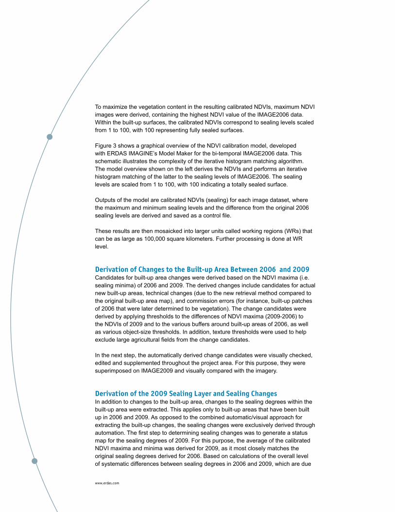
To maximize the vegetation content in the resulting calibrated NDVIs, maximum NDVI images were derived, containing the highest NDVI value of the IMAGE2006 data. Within the built-up surfaces, the calibrated NDVIs correspond to sealing levels scaled from 1 to 100, with 100 representing fully sealed surfaces.

Figure 3 shows a graphical overview of the NDVI calibration model, developed with ERDAS IMAGINE’s Model Maker for the bi-temporal IMAGE2006 data. This schematic illustrates the complexity of the iterative histogram matching algorithm.The model overview shown on the left derives the NDVIs and performs an iterative histogram matching of the latter to the sealing levels of IMAGE2006. The sealing levels are scaled from 1 to 100, with 100 indicating a totally sealed surface.

Outputs of the model are calibrated NDVIs (sealing) for each image dataset, where the maximum and minimum sealing levels and the difference from the original 2006 sealing levels are derived and saved as a control file.

These results are then mosaicked into larger units called working regions (WRs) that can be as large as 100,000 square kilometers. Further processing is done at WR level.

Derivation of Changes to the Built-up Area Between 2006 and 2009Candidates for built-up area changes were derived based on the NDVI maxima (i.e. sealing minima) of 2006 and 2009. The derived changes include candidates for actual new built-up areas, technical changes (due to the new retrieval method compared to the original built-up area map), and commission errors (for instance, built-up patches of 2006 that were later determined to be vegetation). The change candidates were derived by applying thresholds to the differences of NDVI maxima (2009-2006) to the NDVIs of 2009 and to the various buffers around built-up areas of 2006, as well as various object-size thresholds. In addition, texture thresholds were used to help exclude large agricultural fields from the change candidates.

In the next step, the automatically derived change candidates were visually checked, edited and supplemented throughout the project area. For this purpose, they were superimposed on IMAGE2009 and visually compared with the imagery.

Derivation of the 2009 Sealing Layer and Sealing ChangesIn addition to changes to the built-up area, changes to the sealing degrees within the built-up area were extracted. This applies only to built-up areas that have been built up in 2006 and 2009. As opposed to the combined automatic/visual approach for extracting the built-up changes, the sealing changes were exclusively derived through automation. The first step to determining sealing changes was to generate a status map for the sealing degrees of 2009. For this purpose, the average of the calibrated NDVI maxima and minima was derived for 2009, as it most closely matches the original sealing degrees derived for 2006. Based on calculations of the overall level of systematic differences between sealing degrees in 2006 and 2009, which are due

www.erdas.com

to different image acquisition times, the level of sealing differences that could be attributed to real changes of the sealing degree was determined. The level of sealing degree differences was applied along with spatial thresholds to derive change classes of sealing degrees. Four change classes were derived in both change directions, yielding as many as nine sealing change classes overall: four classes each for sealing increase and decrease, and one class of relatively stable areas without attributed sealing changes. Figure 3 shows an example for the result of this operation.

Conclusion An update of the built-up and impervious layers of Europe, covering 5.8 million square kilometers and spanning 38 countries was performed based on IMAGE2009 data. The update methodology was largely automated and was implemented with ERDAS IMAGINE’s Spatial Modeler, a processing engine, and its graphical component, Model Maker. The intuitive graphical interface of the Model Maker proved ideal for developing and distributing the highly interlinked sealing update workflows.

The high degree of automation and the uniform methodology applied by the consortium members ensured a spatially consistent update product with a nominal accuracy of 85 %. Upon request by EEA, the product is currently undergoing a validation through the European Topic Center (ETC). For the near future, further High Resolution (HR) layers covering forests, water, wetlands and grasslands are planned for Europe.

Furthermore, ERDAS spatial modelling technology is continually evolving to better meet user demands for future projects. The Spatial Modeler is now available as a service through ERDAS APOLLO, so models created on the desktop can be published to a server and used across an enterprise. In the future, all of ERDAS IMAGINE’s processing capabilities will be available through the Spatial Modeler. Additionally, emerging technology will enable the Spatial Modeler to expand on

 Figure 3: Example for the sealing differences between 2006 and 2009.

its raster processing capabilities to include vector processing and flow control and to leverage distributed processing. These advances will make it possible to create streamlined workflows for future permeability monitoring and other applications.

ReferencesChen, X., L. Vierling, and D. Deering, A simple and effective radiometric correction method to improve landscape change detection across sensors and across time, Remote Sensing of Environment 98 (2005), 63-79

European Environment Agency European Commission, Joint Research Center, Urban sprawl in Europe - The ignored challenge, EEA Report No 10/2006, Copenhagen, 2006. http://www.eea.europa.eu/publications/eea_report_2006_10/eea_report_10_2006.pdf

Gangkofner, U., Weichselbaum, J., Kuntz, S., Brodksy, L., Larsson. K., De Pasquale, V. (2010): Update of the European High-resolution Layer of Built-up Areas and Soil Sealing 2006 with Image Image2009 Data. Proceedings of the Earsel Symposium 2010, p. 185-192. http://www.earsel.org/symposia/2010-symposium-Paris/Proceedings/EARSeL-Symposium-2010_5-01.pdf

George, X. and C. Homer, Updating the 2001 National Land Cover Database Impervious Surface Products to 2006 using Landsat Imagery Change Detection Methods, Remote Sensing of Environment (2010), doi:10.1016/j.rse.2010.02.018, 11pp

Tinz, M., GMES Fast Track Service Precursor on Land Monitoring, Presentation held at the Geoland 5th Forum (2009). http://www.gmes-geoland.info/events/download/Tinz_ITD0490_EEA-FTSP-g2Forum-0905214_I1.pdf

Copyright © 2011 ERDAS All rights reserved.