MANUSCRIPT 1

Unlimited Sampling from Theory to Practice:Fourier-Prony Recovery and Prototype ADC

Ayush Bhandari, Felix Krahmer and Thomas Poskitt

Abstract

Following the Unlimited Sampling strategy to alleviate the omnipresent dynamic range barrier, we study theproblem of recovering a bandlimited signal from point-wise modulo samples, aiming to connect theoretical guaranteeswith hardware implementation considerations. Our starting point is a class of non-idealities that we observe inprototyping an unlimited sampling based analog-to-digital converter. To address these non-idealities, we provide anew Fourier domain recovery algorithm. Our approach is validated both in theory and via extensive experiments onour prototype analog-to-digital converter, providing the first demonstration of unlimited sampling for data arisingfrom real hardware, both for the current and previous approaches. Advantages of our algorithm include that it isagnostic to the modulo threshold and it can handle arbitrary folding times. We expect that the end-to-end realizationstudied in this paper will pave the path for exploring the unlimited sampling methodology in a number of real worldapplications.

Index Terms

Analog-to-digital, modulo, non-linear reconstruction, Shannon sampling, Prony’s method, super-resolution.

CONTENTS

I Introduction 3I-A Overview of Unlimited Sampling and Reconstruction . . . . . . . . . . . . . . . . . . . . . . 3I-B Related Work . . . . . . . . . . . . . . . . . . . . . . . . . . . . . . . . . . . . . . . . . . . 4I-C Motivation and Contributions . . . . . . . . . . . . . . . . . . . . . . . . . . . . . . . . . . . 5

II Fourier Domain Reconstruction Approach 6II-A Recovery Approach . . . . . . . . . . . . . . . . . . . . . . . . . . . . . . . . . . . . . . . . 7II-B Summary of Recovery Algorithm . . . . . . . . . . . . . . . . . . . . . . . . . . . . . . . . 9

II-B1 Implementation Strategy . . . . . . . . . . . . . . . . . . . . . . . . . . . . . . . 10

III Hardware Experiments 10

IV Conclusions and Take-Home Message 16

References 16

A. Bhandari’s work is supported by the UK Research and Innovation council’s Future Leaders Fellowship program “Sensing BeyondBarriers” (MRC Fellowship award no. MR/S034897/1) and the European Partners Fund. F. Krahmer acknowledges support by the GermanScience Foundation (DFG) in the context of the collaborative research center TR 109.

A. Bhandari and T. Poskitt are with the Dept. of Electrical and Electronic Engineering, Imperial College London, South Kensington,London SW7 2AZ, UK. (Emails: ayush@alum.mit.edu and thomas.poskitt15@imperial.ac.uk)

F. Krahmer is with the Dept. of Mathematics, TU Munich, Boltzmannstraße 3, 85748 Garching, Germany. (Email: felix.krahmer@tum.de)Manuscript Submitted: 20XX.

arX

iv:2

105.

0581

8v1

[cs

.IT

] 1

2 M

ay 2

021

MANUSCRIPT 2

FREQUENTLY USED SYMBOLS

Symbol Definitionλ Analog-to-digital converter (ADC) threshold.Mλ Centered modulo non-linearity.Mλ Generalized or non-ideal modulo non-linearity.tm Folding instant introduced by Mλ.BΩ Space of Ω-bandlimited functions.g (t) Continuous-time, Ω-bandlimited function.γ [k] Point-wise samples of a bandlimited function.y [k] Modulo samples of a bandlimited function.εg (t) Simple function taking values on a 2λ-grid.Rg (t) Simple function taking values on a general grid.∆N Finite-difference operator of order N .γ [k] First order finite-difference of γ [k].gp Fourier series coefficient of function g (t).V Discrete Fourier Transform (DFT) matrix.y [n] Sampled or discrete Fourier transform (DFT).IK Set of K contiguous integers from 0 to K − 1.

MANUSCRIPT 3

I. INTRODUCTION

IN the recent line of work [1]–[3], the authors introduced the Unlimited Sensing Framework (USF). TheUSF allows for the acquisition of signals that are orders of magnitude larger than the dynamic range of the

analog-to-digital converter (ADC) used in the sampling process. Suppose that an ADC can measure up to 2λ volts(peak-to-peak), then any signal with maximum amplitude larger than λ would result in clipped or saturated samples,for which the Nyquist-Shannon sampling theory is no longer applicable. In contrast, the USF exploits a co-designof hardware and algorithms to allow for high-dynamic-range (HDR) signal recovery beyond the threshold of λ.

• On the hardware side, a continuous-time signal is folded via a modulo non-linearity before it is sampled. InFig. 1, we show an oscilloscope screenshot of the HDR input and the modulo-folded output, obtained via ourhardware prototype. This hardware is later used in Section III of the paper to validate the theory presented inthis work.

• On the algorithmic side, one needs to solve the ill-posed inverse problem of recovering a signal from foldedmeasurements. The solution approach of [1]–[3], which capitalizes on certain commutativity properties of themodulo non-linearity, and the associated reconstruction guarantees are reviewed in the next subsection.

A. Overview of Unlimited Sampling and Reconstruction

When working with folded signals as in Fig. 1, the following result shows that a bandlimited function can berecovered from a constant factor oversampling of its modulo samples.

Theorem 1 (Unlimited Sampling Theorem [1]). Let f (t) be a continuous-time function with maximum frequencyωmax (rads/s). Then, a sufficient condition for recovery of f (t) from its modulo samples (up to an additive constant)taken every T seconds apart is T 6 1/ (2ωmaxe) where e is Euler’s constant.

Note that the sampling criterion is independent of λ and only depends on the bandwidth of the signal. This issomewhat surprising and indeed the reconstruction becomes less stable with respect to noise for large amplitudes[3]. Also, the sampling rate required for local reconstruction from a finite set of modulo samples grows in proportionto the dynamic range of the signal, relative to λ, see for example the local reconstruction theorem discussed in [4],[5].

Fig. 1. Hardware demonstration for unlimited sampling [1]–[3]. We show an oscilloscope screen shot plotting a continuous-time function(ground truth, black) and its folded version (pink). The input signal with dynamic range 20V peak-to-peak (≈ 10λ) is folded into a 4.025Vpeak-to-peak, signal. We have tested sampling and recovery of signals as large as 24λ. A live YouTube demonstration is available athttps://youtu.be/prV40WlzHh4.

MANUSCRIPT 4

How does the Unlimited Sampling algorithm [3] work? Let us formally define the centered modulo operationusing the mapping

Mλ : f 7→ 2λ

([[f

2λ+

1

2

]]− 1

2

), [[f ]]

def= f − bfc (1)

where [[f ]] and bfc define the fractional part and floor function, respectively. The recovery procedure for “inverting”the Mλ(·) operator relies on two steps, (i) isolating the higher order finite differences followed by, (ii) stably invertingthe difference operator. The modulo decomposition property (cf. Fig. 4 in [3]) allows us to write,

g (t) = Mλ(g (t)) + εg (t) , εg ∈ 2λZ (2)

where εg is a simple function. Let us fix g ∈ BΩ where BΩ denotes the space of Ω-bandlimited functions. Wedenote the conventional and modulo samples by, γ [k] = g (kT ) and y [k] = Mλ(g (kT )), respectively. Let ∆Ny =∆N−1 (∆y) denote the N th difference operator with (∆y) [k] = y [k + 1] − y [k]. Since ∆Nεg ∈ 2λZ, it followsthat,

Mλ(∆Nεg (kT )) = 0(2)

=⇒ Mλ(∆Nγ) = Mλ(∆Ny). (3)

Oversampling g ∈ BΩ results in highly correlated samples and hence,(∆Nγ

)[k] shrinks as the sampling step T

decreases. Quantitatively, the shrinking effect is explained by the bound, ‖∆Nγ‖∞ 6 (TΩe)N‖g‖∞ in [3] where‖ · ‖∞ denotes the max-norm. For a suitable N (cf. [3]), namely,

N? >

⌈log λ− log βg

log (TΩe)

⌉, βg ∈ 2λZ and βg > ‖g‖∞, (4)

choosing T 6 1/Ωe ensures that ‖∆N?

γ‖∞ 6 λ. Modular arithmetic shows that1 for any sequence s [k], it holdsthat

Mλ(∆Ns) = Mλ(∆N (Mλ(s)). (5)

By choosing N = N?, we have,

T = TUS 6 1/Ωe(5)

=⇒ ∆N?

γ = Mλ(∆N?

y). (6)

The unlimited sampling based recovery algorithm [1] recovers γ from ∆N?

γ and is also stable with respect toquantization noise [3]. The reconstruction works by estimating ∆(N?−n)εγ for n = [0, N?] thus yielding εγ , andfinally, γ = y + εγ , is the recovered signal. The approach in [1], [3],(i) is inherently stable because we are able to exploit the restriction on the range of εγ , that is, εγ ∈ 2λZ.

(ii) exploits properties of bandlimited functions2 to estimate the “unknown constant of integration” for inversion of∆N .

It is precisely this synergistic interplay between (i) and (ii) that allows our approach to treat orders N > 1,distinguishing it with seemingly similar methods3 [6] analogous to Itoh’s method for phase unwrapping [7], thatare restricted to low orders. For further details and comparisons, see [3]. Recovery with higher orders has clearadvantages in the context of applications such as HDR imaging [8], tomography [9], [10] and sensor array processing[11], [12].

B. Related Work

Following our work [1], the problem of sampling and reconstruction of bandlimited and smooth functions, frommodulo samples, has been studied in various contexts. Ordentlich et al. [13] studied recovery from quantized modulosamples, using side-information, from a rate-distortion perspective. In parallel papers, [14] and [15] proved thatbandlimted functions are uniquely characterized by modulo samples, when sampling rate is above the Nyquist rate.In [15], the authors also present a constructive approach, provided that a subset of unfolded samples is known.Unlimited sampling has also been studied in the context of finite-length signals [4], [5], random measurements of

1See Proposition 2 in [3].2In praticular, we use Bernšteın’s inequality. This allows for recovery of the unknown polynomial in the kernel of ∆N , up to a constant.3The key difficulty is that each time the operator ∆ is inverted, an unknown constant in the kernel of ∆ has to be estimated. Also for

N = 1, our method is considerably more stable as these approaches do not capitalize on the stabilizing effect described in (i).

MANUSCRIPT 5

Fig. 2. Example of reconstruction based on data acquired using our prototype US-ADC. Ground truth is shown in shaded yellow. (a) Non-ideal modulo mapping. (b) Unlike in the perfect modulo case, the residue function, or g−Mλ(g), no longer lies on a grid of 2λZ, speciallyat the locations marked by gridlines on the y-axis. The first order difference encodes both non-ideal folds and inaccuracies in terms of asparse representation. (c) By exploiting the sparse structure of the residue, our algorithm that is agnostic to λ is able to recover the residueprecisely. (d) Since g−Mλ(g) 6∈ 2λZ, (3) does not apply and unlimited sampling based recovery [3] yields an erroneous reconstruction. Incontrast, our Fourier domain approach based reconstruction is agnostic to λ and results in a near perfect reconstruction.

sparse signals [16], one-bit [17] and multi-channel sampling [18] as well as wavelet based reconstruction approaches[19]. Recovery guarantees for denoising of modulo samples with bounded and Gaussian noise models were discussedin [20].

Recently, we have have developed USF based recovery methods that are tailored to larger classes of signal spacesand inverse problems. For instance, recovery of multi-dimensional functions on arbitrary lattices was considered in[21]. Functions that belong to spline spaces (e.g. images) were studied in [8]. The modulo Radon transform wasintroduced in [9] and its application to HDR tomography was presented in [10]. Computational sensor array signalprocessing based on USF was presented in [11], [12].

C. Motivation and Contributions

The work presented in this paper is pivoted around the practical aspects of unlimited sampling and the insightsdeveloped from building a prototype USF based ADC.1) Non-Ideal Folding. When implementing the modulo circuit in hardware (see Section III for more details), we

observed that it occasionally exhibits non-ideal foldings. An example output of the circuit with such artifactsis shown Fig. 2(a). More precisely, in Fig. 2(a) some of the folding times are delayed; other types of non-idealfoldings that we have observed includes spurious jumps and inaccuracies in the folding threshold λ. In allthese cases, the residue εg in (2) is still piecewise constant, see for example Fig. 2(b), but no longer satisfiesεg ∈ 2λZ. The consequence is that Mλ(∆Nεg (kT )) 6= 0 in (3) and the reconstruction via (6) is erroneous,see Fig. 2(c)). We attribute the artifacts to electronic limitations such as the maximum rate at which an inputsignal can be folded. As this rate depends on the bandwidth of the input signal, ωmax, an exact implementationmust be carefully calibrated to match ωmax in Theorem 1. In this paper we show that this calibration is notrequired and rather, such limitations can be circumvented algorithmically.

2) Lower Sampling Rates. While TΩe 6 1 guarantees that (6) holds for some N , in practice, for stability reasons,it is desirable that we work with smaller values of the finite-difference order N . To satisfy (4), one then needshigher oversampling. Thus a natural question is whether alternative recovery approaches can allow for recoverywith both moderate oversampling and low values of N .

MANUSCRIPT 6

Contributions: The main contribution of this work is to provide the first validation the unlimited sampling approach,thus taking our theoretical ideas all the way to practice. To do so, we go beyond the conventional literature infundamental ways. On the theory front, we propose a novel, Fourier domain, recovery algorithm that can handle non-idealities and uncertainties introduced by the hardware, while operating at lower sampling rates. On the hardwareend, we develop a custom-designed, USF based prototype ADC, the US-ADC. This is the key to enabling realexperiments. Extensive hardware experiments based on the US-ADC, corroborate the effectivity of our new recoveryapproach. The upshot of our end-to-end sensing pipeline is that we can recover signals as large as 24× the ADCthreshold (λ). Furthermore, our work also validates the first approaches presented in [3].

Concretely, the advantages of our recovery method include that it1) is agnostic to λ and hence, can combat any non-idealities.2) requires computation of ∆1 only; this is specially beneficial in the case of errors. The approach in [3] requires

computation of ∆N which can be sensitive to hardware artifacts.The precise signal model that we are working with consists of periodic, bandlimited signals, i.e., trigonometricpolynomials of finite degree. Note that this model is more restrictive than the infinite dimensional model consideredin previous works; this restriction, however, reflects the practical limitation that one typically samples signals on afinite interval rather than the full real line.

Notation. The sets of real, integer, and complex-valued numbers are denoted by R, Z and C, respectively. Weuse IK = 0, . . . ,K − 1,K ∈ Z+ to denote the set of K contiguous integers while its continuous counterpart isdenoted by 1X (t) , t ∈ R, the indicator function on the domain X . For a τ -periodic function h, we consider therenormalized Fourier series coefficients as given by hm =

∫ τ0 h (t) e−mω0tdt where ω0 = 2π/τ is the fundamental

harmonic. Vectors and matrices are written in bold fonts. The mean squared error or MSE between vectors x andy of length K is defined by

E (x,y)def=

1

K

K−1∑

k=0

|x [k]− y [k] |2. (7)

II. FOURIER DOMAIN RECONSTRUCTION APPROACH

Signal Model. In our work, we consider g ∈ BΩ such that g (t) = g (t+ τ) , ∀t ∈ R. Such signals can be writtenas,

g (t) =∑

|p|6P

gpepω0t, ω0 =

2π

τ, P =

⌈Ω

ω0

⌉(8)

where gp denotes the Fourier series coefficient and g−p = g∗p (Hermitian symmetry) with∑p|gp|2 <∞. Sampling

g (t) with sampling rate T results in K samples γ [k] on the interval [0, τ). To solve for gp in (8), one requiresK > 2P + 1. Wen working with oversampled representation, we write gp in the Fourier domain as,

gp =1

τ

∫ τ0 g (t) e−ω0pt, p ∈ EP,K

0, p ∈ IK \ EP,K, (9)

where the set EP,K is given by,

EP,K = [0, P ] ∪ [K − P,K − 1] , |EP,K | = 2P + 1. (10)

With KT = τ , the critical sampling rate for a P = dΩ/ω0e bandlimited function is T 6 τ/ (2P + 1).

Generalized Modulo Non-linearity. Our non-ideal modulo non-linearity, Mλ(·), corresponds to subtracting apiecewise constant function, with finite discontinuities, from g ∈ BΩ. In formulas, Mλ(·) admits a representationof the form,

g (t) = Mλ(g (t)) + Rg (t) , t ∈ [0, τ) (11)

where the (generalized) residue function is of the form

Rg (t) =∑

m∈Mc [m]1Dm (t), ∪·m1Dm = R, c [m] ∈ R. (12)

MANUSCRIPT 7

<latexit sha1_base64="olZOdvPeDhrwI9ovqJUK4MQpWmI=">AAACbnicbVHbatwwENU6vaTbSzYN9KWUijqFPC32QmkeA33pW7bQTVLWZhnL46yIJBtp3LAIf0Vfmw/rX/QTKm8W2mw6IOlwzhnNaFQ0SjpKkl+DaOfBw0ePd58Mnz57/mJvtP/yzNWtFTgTtartRQEOlTQ4I0kKLxqLoAuF58XVp14//47Wydp8pVWDuYZLIyspgAL17TBrdOGn3eFiFCfjZB38Pkg3IGabmC72B6dZWYtWoyGhwLl5mjSUe7AkhcJumLUOGxBXcInzAA1odLlfd9zx94EpeVXbsAzxNftvhgft3EoXwamBlm5b68n/afOWquPcS9O0hEbcFqpaxanm/fN5KS0KUqsAQFgZeuViCRYEhSEN75TB1gVHQ12gLRq8FrXWYMqsAJu1pkTbD31LWwJl17LEcA5D3l/FZ2VF3XyS8xC+9/n+Ih+nXbfw8STsozjdHvh9cDYZpx/GyZdJfHK8+Yxd9pq9Y0csZR/ZCfvMpmzGBNPsB/vJbga/o1fRm+jtrTUabHIO2J2Ijv4AIxG86w==</latexit>

PPP<latexit sha1_base64="IMD5kf3WvzzT0frE+Vu4UKH6B3g=">AAACcnicbVFNb9QwEPWGr7J8beEGF0OKxIGukpUQPVbigsSBRWLbSptoNXEmXau2E+wJ1crK7+AKP4v/wQ/AWSJBt4xk++m9Gc/oTdEo6ShJfo6iGzdv3b6zd3d87/6Dh48m+49PXN1agQtRq9qeFeBQSYMLkqTwrLEIulB4Wly86/XTr2idrM1n2jSYazg3spICKFD5Qdbown84nB+m3cFqEifTZBv8OkgHELMh5qv90cesrEWr0ZBQ4NwyTRrKPViSQmE3zlqHDYgLOMdlgAY0utxvp+74y8CUvKptOIb4lv23woN2bqOLkKmB1m5X68n/acuWqqPcS9O0hEb8aVS1ilPNewt4KS0KUpsAQFgZZuViDRYEBaPGV9pg60JGQ12gLRq8FLXWYMqsAJu1pkTbG7+jrYGyS1lieMeh7q/is7KibjnLeQjf5/n+Ix+nXbfy8SzckzjdNfw6OJlN0zfT5NMsPj4alrHHnrEX7BVL2Vt2zN6zOVswwb6wb+w7+zH6FT2NnkfD5qLRUPOEXYno9W9zw73p</latexit>

K P 1K P 1K P 1<latexit sha1_base64="XRCHD+r+8j5BMzXoc1yJhd5LRNM=">AAACcHicbVHLatwwFNW4r3T6mjSbQhdV6xRKoYNtCMkykE0gi6bQSQK2GWT5OiOih5GuGwbhz+i2/a7+Rr+g8mSgzaQXJB3OOVdXHFWtFA6T5Ncounf/wcNHW4/HT54+e/5isv3yzJnOcphxI429qJgDKTTMUKCEi9YCU5WE8+rqaNDPv4F1wuivuGyhVOxSi0ZwhoHKd4tWVf7kU9bvzidxMk1WRe+CdA1isq7T+fboc1Eb3inQyCVzLk+TFkvPLAouoR8XnYOW8St2CXmAmilwpV+9uafvA1PTxtiwNNIV+2+HZ8q5paqCUzFcuE1tIP+n5R02B6UXuu0QNL8Z1HSSoqFDALQWFjjKZQCMWxHeSvmCWcYxxDS+NQY6Fxwt9oG2oOGaG6WYrouK2aLTNdgh9g1twbC4FjWEcxz6/iq+qBvs86ykofzg88NFPk77fu7jLOyTON0M/C44y6bp3jT5ksWHB+vP2CKvyTvygaRknxySY3JKZoQTQ76TH+Tn6Hf0KnoTvb2xRqN1zw65VdHHPyilvVk=</latexit>

K 2K 2K 2<latexit sha1_base64="yW/unMdGSSpKv6/y5b3ODC+A0uo=">AAADDHicbVJNb9QwEPWGr7J8dAtHLhYpEgdYJSshekGqhJDgtkhsWymJVo4z2bUaO8GeUK0sXznySzgCF8SVX8CFf4OTrlB325GiPL/3Zjz2OG8qYTCK/g6Ca9dv3Ly1c3t45+69+7ujvQdHpm41hxmvq1qf5MxAJRTMUGAFJ40GJvMKjvPT151+/Am0EbX6gKsGMskWSpSCM/TUfET300bmNi1KtCtnlaOv6PN+pbuV25+Pwmgc9UEvg3gNQrKO6Xxv8Cctat5KUMgrZkwSRw1mlmkUvAI3TFsDDeOnbAGJh4pJMJntj+LoE88UtKy1/xTSnr2YYZk0ZiVz75QMl2Zb68irtKTF8iCzQjUtguLnG5VtRbGm3b3QQmjgWK08YFwL3yvlS6YZR397w41toDXe0aDztAYFZ7yWkqkizZlOW1WA7qaxpS0ZpmeiAP/3aRcEaQCTOKM+bNr1nef2nZvbMHZuwwhXGN944/RZb92oalPzMXf/3RWUmNAwpqkWiyVmbtPrx+2SydrrG7TdSfoGujI2nPjy/h3E21O/DI4m4/jFOHo/CQ8P1i9ihzwij8lTEpOX5JC8JVMyI5x8Jl/Jd/Ij+BJ8C34Gv86twWCd85BsRPD7H6Yh9+o=</latexit>

by [n] = br [n]by [n] = br [n]by [n] = br [n]

Trigonometric Polynomial<latexit sha1_base64="m5w+WjilHg/rDM+lUR5lLxE2m4c=">AAAoN3ic7VpLcxvHER7bSOIwL9k65rIVUkVZoVggRFnKQymZFGm6REsURUoqa0kWHgtgSwsshF1SZKDNMX8j1+Qn5KfklFsq1/yDdH8zszv7Bhz7FqKI3Z3pd/d098yiM/HcIGw2//HBhx81fvDDH33846Wf/PRnP//FtU8+fRH459Ouc9z1PX/6qtMOHM8dO8ehG3rOq8nUaY86nvOy82ab519eONPA9cdH4dXEORm1B2O373bbIQ2dXbu+Yk9GndnYdsd24IT+eRitnF1bbq7/5v7nrc3PreZ6s3lvo7XBN617m3c2rQ0a4b9lof4O/E+u/1nYoid80RXnYiQcMRYh3XuiLQL6vBZ9unfEWxpfExuiKSY0fyJmND+lOxewjojEEn1sohHQ04Rmu+INfQ/oaUb/PN4lDBf4DH1DWGKX+DI/SxwSDPMM6drDbBmtobiisSEkbce07Ny4C9qzxu8bTXG7sdW4S9/6/j59/5burUar8YfGF/T0BY3y3INGs9Gi6+8A06Knrca+0m6pQsfXapR5sxUDslZPXEDfIDUa0OggNRLSfQdWZLteElWfnnyyVlRh0w5B+PQssYNKWI/kGEM6vxaO5eVIqILrElyovF4GMyD52/AIx8hlJSxLxjwl1VHs0zIp2+Rrn2bDSqocoVPAVkGdE4xXE7/sq4C4DWvsIuEC4jgin9RD9lX8V3nvNd1zpFxi9Z3EuCNE+bDGT22MV0eHpjSFRNWwHfqMjPXAq/gIq47jlX1niUd07SPi3HgdBqAZpiDZoleI+xnxYa8yjuTO0fouA3+L4LIjEY2l+ZfjZ7EXw+0VaMUUirStouPhyjZn7H3jqRynq7LBTGzjjvODh/i+qsSbAHZC/0FG6oOSmXJa8so834DCYeq5ymcOxQ5j7FAMc+xO4ophA0risY7SEmOy9Yzm3qIWRLgfwsas9Qo9daA9x2VAUOeQwqGZbFzyqgnBR3rPpm/Olx5oOpBlCAm5BvH4uvgTUYkyOIMc/DqNrVPujggvDe0ink1olyCdDLQHnjY82SPp2RIWpA5pzFKrz4KWXVWV2RoWauiYuFuxnsfEp6dqp4UISewYpLjJSq6vAaw4VhbSMAMFM6iAGYKbTV5zobd81pa/oep5n/6lf7uxzEXSlfl/Rzyj0Ygy4Abyno2MIf3OdNmLN1UM9el+meAi8Rki5kHsxTLqbOce6mFCf6giI4AnZY71MCZpR3GdKKPKUTowaO7ieZ1mHpL2WVmrJZRVPZGuo6JF1xc/JVmdXGGKlgc5QhqxyZrsp7G4TfVlnSDuInZNGOZhI/IGZCPu/8qxTKhq/frIAvPIdIe+F5cpwVpEJg+ZNi8V3/XRl/lYq8zfStHm+wSiziNfi6cpProKyz55RvOROAPXNrzNK5yfTM7VurzIcLhQeXKCnO8h459lIqiKXhs9jabHI0mnOjNycqRk1DQ5H2yhE+vCQ2HNuuec3imJjCK71/mUK10xvZuF9D7LZHQvg5OenSoeaWyp9RPYZlSj7z55JG1XHQsd5Ip9WPIMc2YeKqfo5Sg6yGNRxt/lFMZKcpk17oCOhZn3uEoaFp4lVSvWhWdb4GDF1uexO3NIrvn2wHezhO+p4Vce24y5fT/SHC1khby9/1f+xfkoK4OZid7XUG7nqouOOe4KuWa/V2sjmelirXNf8r42u32lck9LReBMVfRz8dw4B5jBspEw4/LUsFh9VXuTifM8h90M/Wq77BB2Iret9q8aey2WrIpGV0nVqs2TxRJv59b7Wsom9dzDBfjrHi5ETeip7rVMKlmTuJvrY/d2WimlmScfUw0opvw4XtGPSMY1XJ8qC0zo+S39T+fo574rq7eUPFV6cXbfwXrjtWJRreVO8Vw4Nble7pkuKyv/jpLDnOE6oDHlapdVcoZ7CTcTX8aYssZ3IbtZNeqs6OAUZvwt5ZOY3698U3Xql8iX96WWUNJNsq5N+17mm3Q70pNfKz2qzi50HL8DHR9nMoN4365nX2L2acnsAc0/LbAcj8uV9TKDcVQTywmlKXbpR4YNNY0L6Byk+HbVLviFstQwh9WbAyvx7B7wT8l+aSp7RCPf0eypFXbbyMga4xF5r3ivZysdJWQkzH2eSWFLfJPhyb7/Jsdpi3apebjDAopHtMd+TtGR/7DFi9bCMepIluMRdYTPFqLzpITOLtlpETq78Ez+ZKOYxgw7s2RHoOGlXV1kvHr7HlZAH+agtyugtwt88ggrqWptPCmILb8GZ1SA069dg/JUKYvJ70zqKtEzJaWV0y9EpxUW+PJVgTUCVcHHJR5NcqAFeTXtx/EatMSvUx2qnqn3s6Qlz+Pn4T7KcbdiKrKG8OnXdyVn8t6mrKZsYYel64neD2YjUee+rTj3mVm+umoxh4NvxWMSVyvzhFHTNTXmvRpbyjwN4nnecTOUPLsLUUFNaiOS9gKj8r2KSXcCeTSehn0Yw0YFlJJZ1pL7Jr1raYPPBeB6oHeBuOE92g2iJKOFz7nkWwv91iogHbiy2+KPRF0/WaCahuBn+RbpttLikji5Qr7XTDi40MvFezjzdHkFWA+hu5R+GWN63kaXwTrJu67qS+s68iFOXvqIa33SLveTrw1rc37oIT6W4rXDUsi82Cdd0vsxHza5wB5FntH6qI+yV5VnkUu51Ti/d2eGpnK/mqZmPldJyKfwE2WPNvYNDk68e+gvJopb4rtAyR7lYthXbxemNSua32VPcLobqn6/yAem7TuIpBMDW+NpKnVntRxNi/NlC53kKBTxrstio1xfnO65sidyh3hTEdCa4tM5zt7Jibxe0bpLn+V6Z7PK76sMz9pU7wtOU71/ntJxLSW9AyqiJPV6rvYw3Mu7as/iGO9GxhTjPvZqur+vjiSJEaWkkTnLBnW5hvg0/lJlX6lDG9yTmSbWAc+ugK6L/MG4PeS7EO+v5OdGpr728B6pGOssfgdswu9VwOf79jx+GXa27+jRWF91KUNFM7snkd2buQt7V7DbkHRGc1A6E6MSauVeHCFyzTc91Rw41swzo8X5dRfgdypuzcmziqv8xUX6tDC9fr4U+bPTjZTGfMbF11apzmVvbG8ha7dhaY/yufRsm9aZpzRnGdKj3M1V5bWkV5QamR1lutv7Ssx3xpf0lHUU9RnCAU79zK7q/z33fD13+S+DHHV+Esa/YLCEnRuXfVBbbILCBHV/DWOyE+DM+4Cg7lNuZQ+vUdQ21X2kIPVp+QP8ekZCaQoTGm2lRqOza8v6R3JW+c2L1vrG3fXms9byw/vql3Qfi1+KX4mbxOUedVB7FDXHpPOV+Iv4q/jb6t9X/7n6r9V/S9APP1A410Xqb/U//wWIVZJm</latexit>

n 2 (IK1 \ EP,K1) + (K 1) Zn 2 (IK1 \ EP,K1) + (K 1) Zn 2 (IK1 \ EP,K1) + (K 1) Z

<latexit sha1_base64="NrgtXC9N/DR46IHO+oKvkZ/B+Fw=">AAADA3icbVJNb9QwEPWGr7J8dAsHDlwsUiQOqEpWQvRYCSHBbZHYtlIcrRxnsms1doI9oVpZPvJLOAIXxJV/wYV/g7Ndoe62I0V5eu/NeDzjoq2lxST5O4hu3Lx1+87O3eG9+w8e7o72Hh3bpjMCpqKpG3NacAu11DBFiTWctga4Kmo4Kc7e9PrJZzBWNvojLlvIFZ9rWUnBMVCz0ZN91qrCsbJCx+ZcKe6d9n5/NoqTg2QV9CpI1yAm65jM9gZ/WNmIToFGUXNrszRpMXfcoBQ1+CHrLLRcnPE5ZAFqrsDmbnUDT58HpqRVY8Knka7YyxmOK2uXqghOxXFht7WevE7LOqwOcyd12yFocXFQ1dUUG9qPg5bSgMB6GQAXRoZeqVhwwwWGoQ03joHOBkeLPtAGNJyLJoxLl6zghnW6BNMvYUtbcGTnsoTwD2mXBGUBszSnIRzr+y4K997PXJx6v2GEa4xvg3HycmXdqOqY/VT4/+4aKsxonFJm5HyBud/0hp37bLz2hgZdf5NVA30ZF49D+fAO0u2tXwXH44P01UHyYRwfHa5fxA55Sp6RFyQlr8kReUcmZEoE8eQr+U5+RF+ib9HP6NeFNRqscx6TjYh+/wPo+PRi</latexit>

b [n]b [n]b [n]<latexit sha1_base64="PYSBPe/1u0pcmMDD5q7XAFN61pA=">AAADHXicbVJNixQxEM20X+v4sbN69BLsFTzo0D0g7kVYEEFvIzi7C51mSKerZ8J20m2SdhlCfodHf4lH9SJ7WhD/jemeRnZmtyDk5dWrSqUqWV1ybaLo7yC4cfPW7Ts7d4f37j94uDvae3Skq0YxmLGqrNRJRjWUXMLMcFPCSa2AiqyE4+z0bes//gJK80p+MqsaUkEXkhecUeOp+SjeJ7XILMkLY1fOSoff4O5AFlQI2jEv14xqD25/PgqjcdQZvgriHoSot+l8b3BB8oo1AqRhJdU6iaPapJYqw1kJbkgaDTVlp3QBiYeSCtCp7d7m8DPP5LiolF/S4I69HGGp0HolMq8U1Cz1tq8lr/MljSkOUstl3RiQbH1R0ZTYVLhtFM65AmbKlQeUKe5rxWxJFWXGt3O4cQ002itq4zytQMIZq3zvZE4yqkgjc1DteLZ8S2rIGc/B7z7skkNoMEmcYm+WtHVnmf3g5jaMndsQwjXCd144fdFJN7Jaoj9n7r+6hMIkOIwxUXyxNKnb1Ppxu2TSa32Btn1JV0CbxoYTn97/g3h76lfB0WQcvxpHHyfh4UH/I3bQE/QUPUcxeo0O0Xs0RTPE0Ff0Hf1Ev4JvwY/gd3C+lgaDPuYx2rDgzz/hh/8r</latexit>

by [n] = b [n] br [n]by [n] = b [n] br [n]by [n] = b [n] br [n]

<latexit sha1_base64="zp+gwx7Lcs8jjBntauTIuDSKSbA=">AAADA3icbVJNb9QwEPWGr7J8dAsHDlwsUiQOsEpWQvRYCSGBuCwS21aKo5XjTHatxk6wJ1QrK0d+CUfggrjyL7jwb3C2EepuO5Llp/fejMdjZ3UpLUbR30Fw7fqNm7d2bg/v3L13f3e09+DIVo0RMBNVWZmTjFsopYYZSizhpDbAVVbCcXb6utOPP4OxstIfcVVDqvhCy0IKjp6ajx7ts1plTjOpKQML6N6/iNt2fz4Ko3G0DnoZxD0ISR/T+d7gD8sr0SjQKEpubRJHNaaOG5SihHbIGgs1F6d8AYmHmiuwqVvfoKVPPZPTojJ+aaRr9mKG48ralcq8U3Fc2m2tI6/SkgaLg9RJXTcIWpwfVDQlxYp246C5NCCwXHnAhZG+VyqW3HCBfmjDjWOgsd5RY+tpAxrORKUU1znLuGGNzsF0j7ClLTmyM5mD333aBUH5WSdxSn041vWdZe5dO3ehn/6GEa4wvvHG6fO1daOqY/ZT1v53l1BgQsOYMiMXS0zbTW9eYJtMeq9v0HU3WTfQlXHhxJf3/yDefvXL4Ggyjl+Oow+T8PCg/xE75DF5Qp6RmLwih+QtmZIZEaQlX8l38iP4EnwLfga/zq3BoM95SDYi+P0PmPTzeg==</latexit>

n 2 EP,K1n 2 EP,K1n 2 EP,K1

<latexit sha1_base64="nvO49SkUjG/Xk5Ap7d0P3QJKYFk=">AAADG3icdVJNj9MwEHXD11K+unDkYpFF4gAlCWVbbishJBCXItHdleKocpxJa23sBNthVVn5GRz5JRyBC+IIB/4NTreLNqtlpChP770Zj2ecVgXXJgj+9LxLl69cvbZ1vX/j5q3bdwbbd/d1WSsGM1YWpTpMqYaCS5gZbgo4rBRQkRZwkB69bPWDj6A0L+V7s6ogEXQhec4ZNY6aD57ukEqk1mJJuMREaDD27ZOwwcQhwWWtMYFTsml25gM/GL6Y7EajXRwMg2AcRmELovHo2QiHjmnDR5uYzrd7v0hWslqANKygWsdhUJnEUmU4K6Dpk1pDRdkRXUDsoKQCdGLXN2vwQ8dkOC+V+6TBa/ZshqVC65VInVNQs9TntZa8SItrk08Sy2VVG5Ds5KC8LrApcTsmnHEFzBQrByhT3PWK2ZIqyowbZr9zDNTaOSrTOFqBhGNWCkFlRlKqSC0zUO1yzmlLasgxz8D9XdoZod1AHCbYhSVt32lq3zRz67vxd4xwgfGVM04fr62dqpboD2nzz11AbmLsh5govliapOl6s9w0cbTxugZte5N1A20Z60euvHsHp8vG/wf70TB8PgzeRf7eZPMittB99AA9QiEaoz30Gk3RDDH0CX1B39B377P31fvh/Tyxer1Nzj3UCe/3X3QL/Y4=</latexit>

n 2 IK1 \ EP,K1n 2 IK1 \ EP,K1n 2 IK1 \ EP,K1

<latexit sha1_base64="DUhed74/R6kyHQpj0ZywD/00xUE=">AAACbnicdVHbbtQwEPWGW1lu2yLxghAWKVKfVk5YustbJV54o0hsW7SJVo4z6Vq1ncietFpZ+Qpe4cP4Cz4Bp10EreBItkfnnPGMx0WjpEPGfgyiW7fv3L23dX/44OGjx09G2ztHrm6tgLmoVW1PCu5ASQNzlKjgpLHAdaHguDh73+vH52CdrM1nXDeQa35qZCUFx0B92c0aXXjW7S5HMRu/m+2nk33KxoxNkzTpg3Q6eTOhSWB6xGSDw+X24GNW1qLVYFAo7twiYQ3mnluUQkE3zFoHDRdn/BQWITRcg8v9ZccdfR2Ykla1DcsgvWT/zvBcO7fWRXBqjit3U+vJf2mLFqtZ7qVpWgQjrgpVraJY0/75tJQWBKp1CLiwMvRKxYpbLjAMaXitDLQuOBrsAm3BwIWoteamzApus9aUYPuh39BWHLMLWUI4hyHvj+KzssJukeY0wPc+31/k46Trlj5Owz6Kf8+Z/j84SsfJ2zH7lMYHs81nbJHn5BXZIwmZkgPygRySORFEk6/kG/k++Bk9i15EL6+s0WCT85RcQ7T3C2McvQ0=</latexit>

000<latexit sha1_base64="DUhed74/R6kyHQpj0ZywD/00xUE=">AAACbnicdVHbbtQwEPWGW1lu2yLxghAWKVKfVk5YustbJV54o0hsW7SJVo4z6Vq1ncietFpZ+Qpe4cP4Cz4Bp10EreBItkfnnPGMx0WjpEPGfgyiW7fv3L23dX/44OGjx09G2ztHrm6tgLmoVW1PCu5ASQNzlKjgpLHAdaHguDh73+vH52CdrM1nXDeQa35qZCUFx0B92c0aXXjW7S5HMRu/m+2nk33KxoxNkzTpg3Q6eTOhSWB6xGSDw+X24GNW1qLVYFAo7twiYQ3mnluUQkE3zFoHDRdn/BQWITRcg8v9ZccdfR2Ykla1DcsgvWT/zvBcO7fWRXBqjit3U+vJf2mLFqtZ7qVpWgQjrgpVraJY0/75tJQWBKp1CLiwMvRKxYpbLjAMaXitDLQuOBrsAm3BwIWoteamzApus9aUYPuh39BWHLMLWUI4hyHvj+KzssJukeY0wPc+31/k46Trlj5Owz6Kf8+Z/j84SsfJ2zH7lMYHs81nbJHn5BXZIwmZkgPygRySORFEk6/kG/k++Bk9i15EL6+s0WCT85RcQ7T3C2McvQ0=</latexit>

000

<latexit sha1_base64="olZOdvPeDhrwI9ovqJUK4MQpWmI=">AAACbnicbVHbatwwENU6vaTbSzYN9KWUijqFPC32QmkeA33pW7bQTVLWZhnL46yIJBtp3LAIf0Vfmw/rX/QTKm8W2mw6IOlwzhnNaFQ0SjpKkl+DaOfBw0ePd58Mnz57/mJvtP/yzNWtFTgTtartRQEOlTQ4I0kKLxqLoAuF58XVp14//47Wydp8pVWDuYZLIyspgAL17TBrdOGn3eFiFCfjZB38Pkg3IGabmC72B6dZWYtWoyGhwLl5mjSUe7AkhcJumLUOGxBXcInzAA1odLlfd9zx94EpeVXbsAzxNftvhgft3EoXwamBlm5b68n/afOWquPcS9O0hEbcFqpaxanm/fN5KS0KUqsAQFgZeuViCRYEhSEN75TB1gVHQ12gLRq8FrXWYMqsAJu1pkTbD31LWwJl17LEcA5D3l/FZ2VF3XyS8xC+9/n+Ih+nXbfw8STsozjdHvh9cDYZpx/GyZdJfHK8+Yxd9pq9Y0csZR/ZCfvMpmzGBNPsB/vJbga/o1fRm+jtrTUabHIO2J2Ijv4AIxG86w==</latexit>

PPP<latexit sha1_base64="IMD5kf3WvzzT0frE+Vu4UKH6B3g=">AAACcnicbVFNb9QwEPWGr7J8beEGF0OKxIGukpUQPVbigsSBRWLbSptoNXEmXau2E+wJ1crK7+AKP4v/wQ/AWSJBt4xk++m9Gc/oTdEo6ShJfo6iGzdv3b6zd3d87/6Dh48m+49PXN1agQtRq9qeFeBQSYMLkqTwrLEIulB4Wly86/XTr2idrM1n2jSYazg3spICKFD5Qdbown84nB+m3cFqEifTZBv8OkgHELMh5qv90cesrEWr0ZBQ4NwyTRrKPViSQmE3zlqHDYgLOMdlgAY0utxvp+74y8CUvKptOIb4lv23woN2bqOLkKmB1m5X68n/acuWqqPcS9O0hEb8aVS1ilPNewt4KS0KUpsAQFgZZuViDRYEBaPGV9pg60JGQ12gLRq8FLXWYMqsAJu1pkTbG7+jrYGyS1lieMeh7q/is7KibjnLeQjf5/n+Ix+nXbfy8SzckzjdNfw6OJlN0zfT5NMsPj4alrHHnrEX7BVL2Vt2zN6zOVswwb6wb+w7+zH6FT2NnkfD5qLRUPOEXYno9W9zw73p</latexit>

K P 1K P 1K P 1

<latexit sha1_base64="DUhed74/R6kyHQpj0ZywD/00xUE=">AAACbnicdVHbbtQwEPWGW1lu2yLxghAWKVKfVk5YustbJV54o0hsW7SJVo4z6Vq1ncietFpZ+Qpe4cP4Cz4Bp10EreBItkfnnPGMx0WjpEPGfgyiW7fv3L23dX/44OGjx09G2ztHrm6tgLmoVW1PCu5ASQNzlKjgpLHAdaHguDh73+vH52CdrM1nXDeQa35qZCUFx0B92c0aXXjW7S5HMRu/m+2nk33KxoxNkzTpg3Q6eTOhSWB6xGSDw+X24GNW1qLVYFAo7twiYQ3mnluUQkE3zFoHDRdn/BQWITRcg8v9ZccdfR2Ykla1DcsgvWT/zvBcO7fWRXBqjit3U+vJf2mLFqtZ7qVpWgQjrgpVraJY0/75tJQWBKp1CLiwMvRKxYpbLjAMaXitDLQuOBrsAm3BwIWoteamzApus9aUYPuh39BWHLMLWUI4hyHvj+KzssJukeY0wPc+31/k46Trlj5Owz6Kf8+Z/j84SsfJ2zH7lMYHs81nbJHn5BXZIwmZkgPygRySORFEk6/kG/k++Bk9i15EL6+s0WCT85RcQ7T3C2McvQ0=</latexit>

000

Bandlimited Part

Trigonometric Polynomial

<latexit sha1_base64="NrgtXC9N/DR46IHO+oKvkZ/B+Fw=">AAADA3icbVJNb9QwEPWGr7J8dAsHDlwsUiQOqEpWQvRYCSHBbZHYtlIcrRxnsms1doI9oVpZPvJLOAIXxJV/wYV/g7Ndoe62I0V5eu/NeDzjoq2lxST5O4hu3Lx1+87O3eG9+w8e7o72Hh3bpjMCpqKpG3NacAu11DBFiTWctga4Kmo4Kc7e9PrJZzBWNvojLlvIFZ9rWUnBMVCz0ZN91qrCsbJCx+ZcKe6d9n5/NoqTg2QV9CpI1yAm65jM9gZ/WNmIToFGUXNrszRpMXfcoBQ1+CHrLLRcnPE5ZAFqrsDmbnUDT58HpqRVY8Knka7YyxmOK2uXqghOxXFht7WevE7LOqwOcyd12yFocXFQ1dUUG9qPg5bSgMB6GQAXRoZeqVhwwwWGoQ03joHOBkeLPtAGNJyLJoxLl6zghnW6BNMvYUtbcGTnsoTwD2mXBGUBszSnIRzr+y4K997PXJx6v2GEa4xvg3HycmXdqOqY/VT4/+4aKsxonFJm5HyBud/0hp37bLz2hgZdf5NVA30ZF49D+fAO0u2tXwXH44P01UHyYRwfHa5fxA55Sp6RFyQlr8kReUcmZEoE8eQr+U5+RF+ib9HP6NeFNRqscx6TjYh+/wPo+PRi</latexit>

b [n]b [n]b [n]

<latexit sha1_base64="MgK8B5O3+lgeugBVhAk0RGxeZRY=">AAAC/nicbVJNa9wwENW6X+n2a5MeexF1Cj2UxV4ozTEQCu1tC90kYJtFlse7IpbsSuMmixD0l/TY9lJ67Q/ppf+m8saU7CYDQsN7b0ZPI+VNJQxG0d9BcOv2nbv3du4PHzx89PjJaHfv2NSt5jDjdVXr05wZqISCGQqs4LTRwGRewUl+dtTxJ59BG1Grj7hqIJNsoUQpOEMPzUd7+2kjc5sWJdqVs8q5/fkojMbROuj1JO6TkPQxne8O/qRFzVsJCnnFjEniqMHMMo2CV+CGaWugYfyMLSDxqWISTGbX5h194ZGClrX2SyFdo1crLJPGrGTulZLh0mxzHXgTl7RYHmRWqKZFUPzyoLKtKNa0mwQthAaO1conjGvhvVK+ZJpx9PMabhwDrfGKBp2HNSg457WUTBVpznTaqgJ0N/8tbskwPRcF+N2XXSGkAUzijPqwaec7z+17N7dh7NyGEG4QvvXC6au1dKOrTc2n3P1XV1BiQsOYploslpi5Ta1/bpdMeq03aLubrA10bWw48e39P4i3X/16cjwZx6/H0YdJeHjQ/4gd8ow8Jy9JTN6QQ/KOTMmMcHJBvpLv5EfwJfgW/Ax+XUqDQV/zlGxE8PsfNsbySg==</latexit>

by [n]by [n]by [n]

<latexit sha1_base64="3xnyo36TOvOwoz6JCcjlARtjzYU=">AAAC/3icbVJNb9QwEPWGj5bla0uPXCxSJA6wSlZC9FgJIcFtkdi2UhKtHGeyazV2gj1ptbJ84JdwBC6IK/+DC/8GJ12h7rYjWX6a92b87HHeVMJgFP0dBLdu37m7s3tveP/Bw0ePR3tPjk3dag4zXle1Ps2ZgUoomKHACk4bDUzmFZzkZ287/uQctBG1+oSrBjLJFkqUgjP0qflo/+BV2sjcpkWJVjurnDuYj8JoHPVBr4N4DUKyjul8b/AnLWreSlDIK2ZMEkcNZpZpFLwCN0xbAw3jZ2wBiYeKSTCZ7d07+txnClrW2i+FtM9erbBMGrOSuVdKhkuzzXXJm7ikxfIws0I1LYLilweVbUWxpt1T0EJo4FitPGBcC++V8iXTjKN/sOHGMdAar2jQ+bQGBRe8lpKpIs2ZTltVgO4GsMUtGaYXogC/+7IrhDSASZxRHzbtfOe5/eDmNoyd2xDCDcJ3Xjh92Us3utrUfM7df3UFJSY0jGmqxWKJmdvU+nG7ZLLWeoO2u0lvoGtjw4lv7/9BvD316+B4Mo5fj6OPk/DocP0jdslT8oy8IDF5Q47IezIlM8LJinwl38mP4EvwLfgZ/LqUBoN1zT7ZiOD3P7/v8no=</latexit>

br [n]br [n]br [n]

<latexit sha1_base64="GmLv7xnehuoUbgv+lGhhy0I4rCg=">AAAC/nicbVJNa9wwENW6X+n2a5MeexF1Cj2UxV4ozTEQCu1tC90kYJtFlse7IpbsSuMmixD0l/TY9lJ67Q/ppf+m8saU7CYDQsN7b0ZPI+VNJQxG0d9BcOv2nbv3du4PHzx89PjJaHfv2NSt5jDjdVXr05wZqISCGQqs4LTRwGRewUl+dtTxJ59BG1Grj7hqIJNsoUQpOEMPzUd7+2kjc5sWJVrtrHJufz4Ko3G0Dno9ifskJH1M57uDP2lR81aCQl4xY5I4ajCzTKPgFbhh2hpoGD9jC0h8qpgEk9m1eUdfeKSgZa39UkjX6NUKy6QxK5l7pWS4NNtcB97EJS2WB5kVqmkRFL88qGwrijXtJkELoYFjtfIJ41p4r5QvmWYc/byGG8dAa7yiQedhDQrOeS0lU0WaM522qgDdzX+LWzJMz0UBfvdlVwhpAJM4oz5s2vnOc/vezW0YO7chhBuEb71w+mot3ehqU/Mpd//VFZSY0DCmqRaLJWZuU+uf2yWTXusN2u4mawNdGxtOfHv/D+LtV7+eHE/G8etx9GESHh70P2KHPCPPyUsSkzfkkLwjUzIjnFyQr+Q7+RF8Cb4FP4Nfl9Jg0Nc8JRsR/P4HJOvyQw==</latexit>

br [n]br [n]br [n]

Fig. 3. Fourier domain partitioning of the bandlimited signal and the non-ideal folding instants given by (15).

Unlike in [3], we make no assumptions on the coefficients c [m] related to the residue function Rg (t). Note thatMλ(·) includes the exact modulo operation as a special case and hence our algorithm is backwards compatiblewith the sampling model in [3].

A. Recovery Approach

Letting δ denote the Dirac distribution and

y [k]def= ∆y [k] , γ [k]

def= ∆γ [k] , and r

def= ∆Rγ (kT ) , (13)

respectively, we note that (11) implies

k ∈ IK , y [k] = γ [k]− r [k]

= γ [k]−∑

m∈Mc [m] δ (kT − tm) (14)

where tm ∈ (TZ) ∩ [0, τ) are the unknown folding instants. The size of the set M depends on the dynamic rangeof the signal relative to the threshold λ. Since c [m] 6∈ 2λZ, the contribution due to Rg cannot be removed bynon-linear filtering of the amplitudes using a modulo non-linearity as in (3), which is a key ingredient of the methodin [3]. A classical alternative would be to filter out the “impulsive” component r [k] = (∆Rγ) [k] using the medianfilter. However, this yields an inexact solution due to the nature of the median filter and is not considered in thispaper.

Instead, given K modulo samples y [k] , k ∈ IK , we exploit the fact that (14) can be partitioned in the Fourierdomain as,

y [n] =

γ [n]− r [n] n ∈ (EP,K−1) + (K − 1)Z−r [n] n ∈ (IK−1 \ EP,K−1) + (K − 1)Z

(15)

where y [n], the sampled or discrete Fourier transform (DFT) of y [k], is given by,

y [n]def=

∑

k∈IK−1

y [k] e−ω0nk, ω0 =2π

K − 1. (16)

The Fourier domain partition in terms of the DFT coefficients distributed over the two sets,• n ∈ (EP,K−1) + (K − 1)Z (bandlimited part) and,• n ∈ (IK−1 \ EP,K−1) + (K − 1)Z (modulo part)

MANUSCRIPT 8

is schematically explained in Fig. 3. In vector-matrix notation, we can re-write (16) as,

ydef= Vy, [V]n,k = e−(

2π

K−1)nk, k ∈ IK−1 (17)

where V ∈ C(K−1)×(K−1) is the DFT matrix4 and y is the DFT vector corresponding to the first-order finite-difference samples y. In (15) and also as shown in Fig. 3, we have y [n] = −r [n] , ∀n ∈ IK−1 \ EP,K−1 and thissimplifies to a sum of complex exponentials,

r [n] =∑

k∈IK−1

∑

m∈Mc [m] δ (kT − tm) e−ω0nk

=∑

m∈Mc [m] e−

ω0n

Ttm (18)

with M = |M| terms. Estimating the unknown parameters in (18) boils down to the spectral estimation problem [22].In the area of error correction coding and impulse cancellation, Wolf [23] first observed that the non-bandlimitedspikes (or r [k]) being a parametric function, can be curve-fitted (e.g. using Prony’s method) on the “out-of-band”interval, namely, IK−1 \ EP,K−1 in the Fourier domain. This approach was also used for impulse noise removalfrom images [24] as well as bandlimited functions, in the context of Fourier [25] and generalized-Fourier domain[26] sampling theory.

In our case, we notice that (ω) Rg (ω) or equivalently r [n] in (18) is the contribution due to non-bandlimitedspikes. To see the approach in action, let us define a polynomial PM (z) , z ∈ Z of degree M = |M|,

PM (z) =

M−1∏

m=0

(1− ξm

z

)=

M∑

n=0

p [n]z−k (19)

with, roots (PM (z)) = ξmM−1m=0 , ξm = e−

ω0Ttm . (20)

To evaluate the roots of the polynomial PM (z), one starts with identification of the filter coefficients5 p [m]M−1m=0

using Prony’s Method. On any interval of size 2M , we note that (p ∗ r) [n] = 0, which is because,

(p ∗ r) [l] =

M∑

n=0

p [n]r [l − n]

(18)=

M−1∑

m=0

c [m]

M∑

n=0

p [n] eω0Tntme−

ω0Tltm

(19)=

M−1∑

m=0

c [m]PM

(e−

ω0Ttm)

︸ ︷︷ ︸PM (ξm)=0

e−ω0Tltm = 0. (21)

This leads to a recipe for evaluation of unknown filter p = [ p [0] , · · · , p [M ] ]> with p [M ] = 1. Algorithmically,(21) implies that the coefficients of the unknown M–tap FIR filter, p are in the kernel of a Toeplitz matrixcomprising of out-of-band samples of y [n]. More precisely, for a given vector x, let us define a Toeplitz matrix6

TM (x) ∈ CM×(M+1) as,

TM (x)def=

x [0] x [−1] · · · x [−M ]

x [1] x [0] · · · x [1−M ]...

.... . .

...x [M − 1] x [M − 2] · · · x [−1]

. (22)

4We remind the reader that starting with K modulo samples, the operation y [k] = ∆y [k] results in a loss of sample and hence the squarematrix V has a dimension (or rank) of K − 1.

5We use M unknowns of p [m] instead of M + 1 as given by (19) as we normalize p [M ] = 1.6In MATLAB, given a vector x defined by 2M contiguous samples, namely, x[-M+L] · · · x[M-1+L] where L is any integer-

valued translate, the corresponding toeplitz matrix TM (x) is conveniently obtained by defining the function handle T = @(x,M)

toeplitz(x(M+1:end),x(M+1:-1:1)).

MANUSCRIPT 9

Then, (21) amounts to,

p ∈ ker (TM (r)) ⇐⇒ TM (r)p = 0. (23)

By construction, TM (r) requires any 2M , contiguous samples for identifying M = |M| folds of the modulonon-linearity. As per our definition in (15), r [n] is isolated on the set IK−1 \ EP,K−1. For the estimation of p in(23), the requirement is that the cardinality of the set IK−1 \ EP,K−1 is larger than 2M . From Fig. 3, we see that|IK−1 \ EP,K−1| = K − 2P − 2 and this translates to the condition,

K − 2P − 2 > 2M ⇐⇒ K > 2 (P +M + 1)

With KT = τ , the sampling density criterion,

T = TFD 6τ

2 (P +M + 1), P =

⌈Ω

ω0

⌉(24)

guarantees the recovery of the M folding instants tmM−1m=0 introduced by the non-ideal operator Mλ(·). We

formalize our recovery guarantee in the following theorem.

Theorem 2 (Fourier Domain Reconstruction). Let g ∈ BΩ be a τ -periodic function. Suppose that we are given Kmodulo samples of y [k] = Mλ(g (kT )) folded at most M times. Then a sufficient condition for recovery of g (t)from y [k] (up to a constant) is that, T 6 τ/K and K > 2

(⌈Ωτ2π

⌉+M + 1

).

Proof. Note that, by (15) one has that

y [n] = −r [n] , ∀n ∈ (IK−1 \ EP,K−1) + (K − 1)Z.

Then, observing that only such n appear on the right hand side of (22), we obtain from (23) that p ∈ ker(TM

(y))

.Given that TM

(y)

has rank M (this follows from the Vandermonde decomposition of Toeplitz matrices, similarto the Carathéodory–Fejér decomposition, cf. [27]), this implies that p = νp for some ν ∈ C and p as obtainedin step 4b) of Algorithm 1. Consequently, the roots of ξm of PM (z) agree with the roots ξm of PM (z) and onehas tm = tm up to index permutation. Once the exponents have been identified, plugging (18) into (15) yields alinear system which can be solved by least-squares minimization as in Step 4e). This implies that c [m] = c [m]and hence r [k] = r [k], and therefore r [k] = r [k] (up to an additive constant). Together with the modulo samples,these residuals allow for the recovery of the unfolded samples, which completes the proof.

Reconstruction without Periodicity. Recall that the periodicity assumption made in our paper enables a practicalapproach for recovery of signals from folded measurements. A theoretical reconstruction guarantee when infinitesamples are available, however, can also be obtained for signals that are not periodic via the discrete-time Fouriertransform (DTFT). Then the requirement will be to have a sampling density high enough to ensure that in theDTFT, the shift between the aliased copies of the frequency support is at least Ω + 2M + 1.

B. Summary of Recovery Algorithm

Here, we qualitatively summarize the rationale of Algorithm 1. When the sampling criterion in (24) is satisfied,our recovery method can be applied to “unfold” the non-ideal, modulo samples. Starting with K folded samplesof the bandlimited function in (8), we compute the first-difference y = ∆y (cf. (13)). Then, we apply the DFTon the vector y consisting of K − 1 samples, yielding y in (17). According to (15), the DFT coefficients definedfor n ∈ (IK−1 \ EP,K−1) + (K − 1)Z are solely attributed to the unknown folding parameters c [m] , tmm∈Mof Rg (t) in (12). Hence, in the Fourier domain, we define [z]n =

[y]n, ∀n ∈ IK−1 \ EP,K−1 which follows the

parametric representation in (18). Given M = |M|, estimation of c [m] , tm boils down to the classical spectralestimation problem [22]. Concretely, this is implemented in step 4) of Algorithm 1 yielding estimates c [m] , tmwhich are used to estimate r [k] (cf. step 5)). To map r [k]→ r [k], we need to invert the first-difference operatorand this is carried out in (cf. step 6). Combining r [k] with modulo samples y [k] in accordance with (14) yieldsbandlimited samples γFD [k] (cf. step 7)). Low-pass filtering the same results in the continuous-time function g ∈ BΩ.

MANUSCRIPT 10

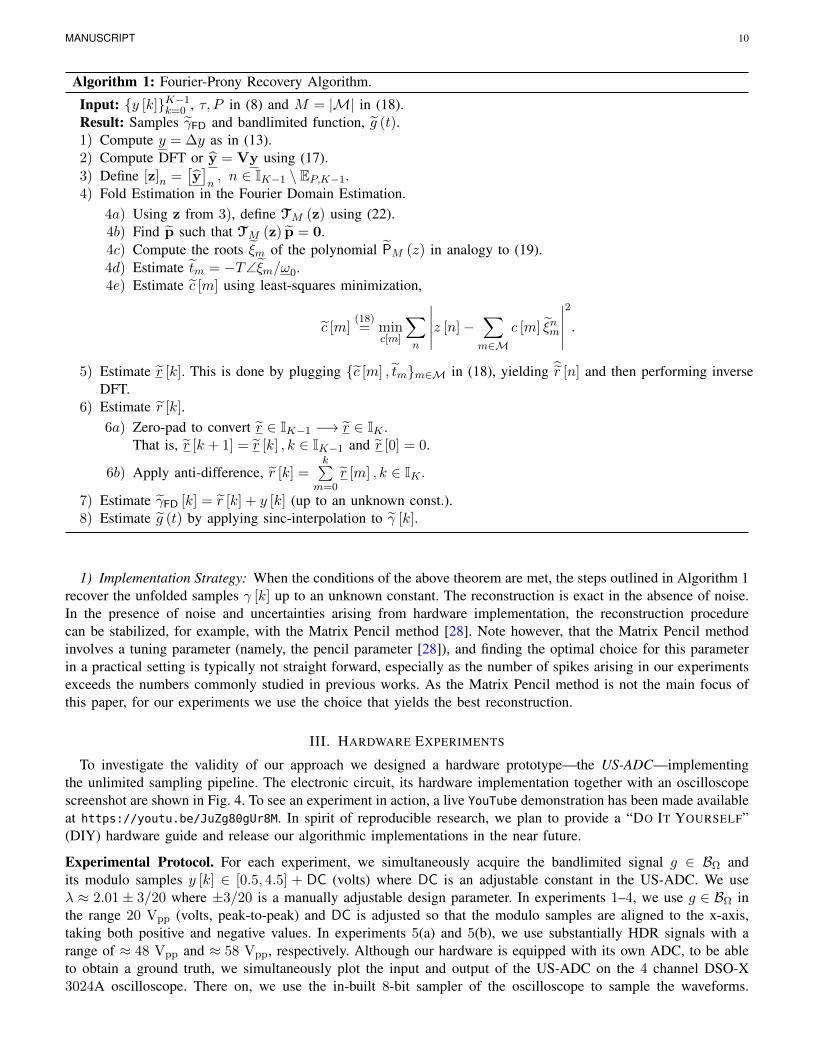
Algorithm 1: Fourier-Prony Recovery Algorithm.

Input: y [k]K−1k=0 , τ, P in (8) and M = |M| in (18).

Result: Samples γFD and bandlimited function, g (t).1) Compute y = ∆y as in (13).2) Compute DFT or y = Vy using (17).3) Define [z]n =

[y]n, n ∈ IK−1 \ EP,K−1.

4) Fold Estimation in the Fourier Domain Estimation.4a) Using z from 3), define TM (z) using (22).4b) Find p such that TM (z) p = 0.4c) Compute the roots ξm of the polynomial PM (z) in analogy to (19).4d) Estimate tm = −T∠ξm/ω0.4e) Estimate c [m] using least-squares minimization,

c [m](18)= min

c[m]

∑

n

∣∣∣∣∣z [n]−∑

m∈Mc [m] ξnm

∣∣∣∣∣

2

.

5) Estimate r [k]. This is done by plugging c [m] , tmm∈M in (18), yielding r [n] and then performing inverseDFT.

6) Estimate r [k].6a) Zero-pad to convert r ∈ IK−1 −→ r ∈ IK .

That is, r [k + 1] = r [k] , k ∈ IK−1 and r [0] = 0.

6b) Apply anti-difference, r [k] =k∑

m=0r [m] , k ∈ IK .

7) Estimate γFD [k] = r [k] + y [k] (up to an unknown const.).8) Estimate g (t) by applying sinc-interpolation to γ [k].

1) Implementation Strategy: When the conditions of the above theorem are met, the steps outlined in Algorithm 1recover the unfolded samples γ [k] up to an unknown constant. The reconstruction is exact in the absence of noise.In the presence of noise and uncertainties arising from hardware implementation, the reconstruction procedurecan be stabilized, for example, with the Matrix Pencil method [28]. Note however, that the Matrix Pencil methodinvolves a tuning parameter (namely, the pencil parameter [28]), and finding the optimal choice for this parameterin a practical setting is typically not straight forward, especially as the number of spikes arising in our experimentsexceeds the numbers commonly studied in previous works. As the Matrix Pencil method is not the main focus ofthis paper, for our experiments we use the choice that yields the best reconstruction.

III. HARDWARE EXPERIMENTS

To investigate the validity of our approach we designed a hardware prototype—the US-ADC—implementingthe unlimited sampling pipeline. The electronic circuit, its hardware implementation together with an oscilloscopescreenshot are shown in Fig. 4. To see an experiment in action, a live YouTube demonstration has been made availableat https://youtu.be/JuZg80gUr8M. In spirit of reproducible research, we plan to provide a “DO IT YOURSELF”(DIY) hardware guide and release our algorithmic implementations in the near future.

Experimental Protocol. For each experiment, we simultaneously acquire the bandlimited signal g ∈ BΩ andits modulo samples y [k] ∈ [0.5, 4.5] + DC (volts) where DC is an adjustable constant in the US-ADC. We useλ ≈ 2.01± 3/20 where ±3/20 is a manually adjustable design parameter. In experiments 1–4, we use g ∈ BΩ inthe range 20 Vpp (volts, peak-to-peak) and DC is adjusted so that the modulo samples are aligned to the x-axis,taking both positive and negative values. In experiments 5(a) and 5(b), we use substantially HDR signals with arange of ≈ 48 Vpp and ≈ 58 Vpp, respectively. Although our hardware is equipped with its own ADC, to be ableto obtain a ground truth, we simultaneously plot the input and output of the US-ADC on the 4 channel DSO-X3024A oscilloscope. There on, we use the in-built 8-bit sampler of the oscilloscope to sample the waveforms.

MANUSCRIPT 11

(a) Printed Circuit Board (b) Hardware Prototype (c) Input and Output on an Oscilloscope

Continuous-time Input SignalContinuous-time Input Signal Live Demo https://youtu.be/JuZg80gUr8MContinuous-time Modulo Output

Low Res

Fig. 4. Hardware prototype for unlimited sensing framework. Our initial design is capable of folding a signal that is as large as 24λ and asshown in Section III, we have tested recovery of signals as large as 48 Vpp and 58 Vpp, respectively. (a) Printed circuit board. (b) Electronicimplementation that transforms a continuous-time input signal into a continuous-time modulo output. (c) Live screen shot of the oscilloscopeplotting the output of a conventional ADC (yellow) and USF based ADC (pink) signal. When the input signal exceeds the oscilloscope’sdynamic range, the oscilloscope’s inbuilt ADC saturates. However, the output signal from our circuit continues to fold. A live YouTubedemonstration of this hardware experiment is available at https://youtu.be/JuZg80gUr8M.

Reflecting the 8-bit resolution, the samples are effectively quantized by an 8-bit, uniform quantizer and hence, themeasurements are corrupted by quantization noise following the model described in [3]. For each experiment, wereport the numerical values for,• the experimental sampling rate T and TFD in (24) which is the sampling criterion required by Theorem 2. Where

needed, we also report TUS that guarantees that (6) holds.• the dynamic range of the input signal (ργ) and the modulo samples (ρy) where ρz = max z [k]−min z [k]. The

ratio ργ/ρy provides a measure of hight-dynamic-range recovery, independent of threshold λ.The bandwidth parameter P in (8) is estimated from the ground truth. Since experimental data may not be exactlyperiodic, we use a slightly higher P so that the complex exponentials are well isolated in Step 3) of Algorithm 1and one obtains an accurate reconstruction. We assume that M = |M| is given and we use the matrix pencil method[28] in Step 4) of Algorithm 1 (cf. Section II-B1). For performance evaluation, we compute the mean squared error(MSE) of the reconstruction defined in (7). We compare the following metrics.• E(γ, γFD) the reconstruction MSE obtained by using our proposed approach in Algorithm 1.• E(γ, γUS), the reconstruction MSE resulting from the unlimited sampling algorithm [3] applied to modulo samples

with a hardwired threshold value of λ = 2.01.• E(γ, γUSopt), the reconstruction MSE for the identical circuit design, but resulting from the unlimited sampling

algorithm with a parameter λopt that is different from the hardwired modulo threshold λ = 2.01, namely,

λopt = minλ

K−1∑

k=0

∣∣γ [k]− USRecλ

(y) [k]∣∣2 (25)

where γUS [k] = USRecλ

(y) [k] is the reconstruction due to unlimited sampling algorithm [3], for a given λ. Therationale behind this choice is that in practice, where occasionally non-ideal folds may appear (cf. Fig. 2(a) andthe residue depicted in Fig. 2(b)), the hardwired threshold λ will not always be the optimal parameter choice;in contrast (25) will yield an optimal choice by design.

For all experiments, we use calibration to estimate the unknown offset arising from Step 6) of Algorithm 1. Theexperimental parameters and results are summarized in Table I.

Experiment 1: Backwards Compatibility with the Unlimited Sampling Approach. The goal of this experimentis to show that in its finite dimensional setting, our recovery approach is backwards compatible with the unlimitedsampling approach. For this experiment, we use modulo samples of a randomly generated trigonometric polynomialshown in Fig. 1. The experimental data and the corresponding recovery results are shown in Fig. 5. The signal

MANUSCRIPT 12

TABLE ISUMMARY OF EXPERIMENTAL PARAMETERS AND PERFORMANCE EVALUATION

Exp. Fig. No. T TFD K τ P ργ ρy M E(γ, γFD) E(γ, γUS) E(γ, γUSopt) λopt

(µs) (µs) (ms)⌈

Ωω0

⌉(V) (V) (Reconstruction MSE)

1 1, 5 132.03 517.86 455 60.07 37 19.87 3.89 20 0.384× 10−3 2.39× 10−3 0.251× 10−3 2.042 2(a), 6 4 21.652 249 0.996 15 7.71 4.12 7 0.343× 10−3 3.7 18.7× 10−3 1.483 7 1000 2426.8 199 199 14 19.61 3.99 26 5.92× 10−3 3.38 7.01 0.834 8 81.25 144.25 245 19.91 20 20.5 3.97 48 9.38× 10−3 1.416× 10−2 — —

5(a) 9 108.49 407.15 1291 140.1 7 ≈ 48 4.26 161 — — — —5(b) 10 70 260.31 357 24.99 3 57.6 5.44 44 0.3405 1.0857 0.4768 2.07

• T is the sampling rate of the ADC while TFD is the sampling rate criterion in Theorem 2. • ργ refers to the dynamic range of input signal (ground truth) and iscomputed using ργ = max γ [k]−min γ [k]. Similarly, the output signal dynamic range ρy refers to the modulo samples y [k]. • E(γ, γFD) refers to the MSE due toreconstruction using the proposed Fourier domain approach. • E(γ, γUS) refers to the MSE due to reconstruction using unlimited sampling approach with λ = 2.01.• E(γ, γUSopt

)refers to the MSE due to reconstruction using unlimited sampling approach with λopt obtained by (25).

<latexit sha1_base64="m5w+WjilHg/rDM+lUR5lLxE2m4c=">AAAoN3ic7VpLcxvHER7bSOIwL9k65rIVUkVZoVggRFnKQymZFGm6REsURUoqa0kWHgtgSwsshF1SZKDNMX8j1+Qn5KfklFsq1/yDdH8zszv7Bhz7FqKI3Z3pd/d098yiM/HcIGw2//HBhx81fvDDH33846Wf/PRnP//FtU8+fRH459Ouc9z1PX/6qtMOHM8dO8ehG3rOq8nUaY86nvOy82ab519eONPA9cdH4dXEORm1B2O373bbIQ2dXbu+Yk9GndnYdsd24IT+eRitnF1bbq7/5v7nrc3PreZ6s3lvo7XBN617m3c2rQ0a4b9lof4O/E+u/1nYoid80RXnYiQcMRYh3XuiLQL6vBZ9unfEWxpfExuiKSY0fyJmND+lOxewjojEEn1sohHQ04Rmu+INfQ/oaUb/PN4lDBf4DH1DWGKX+DI/SxwSDPMM6drDbBmtobiisSEkbce07Ny4C9qzxu8bTXG7sdW4S9/6/j59/5burUar8YfGF/T0BY3y3INGs9Gi6+8A06Knrca+0m6pQsfXapR5sxUDslZPXEDfIDUa0OggNRLSfQdWZLteElWfnnyyVlRh0w5B+PQssYNKWI/kGEM6vxaO5eVIqILrElyovF4GMyD52/AIx8hlJSxLxjwl1VHs0zIp2+Rrn2bDSqocoVPAVkGdE4xXE7/sq4C4DWvsIuEC4jgin9RD9lX8V3nvNd1zpFxi9Z3EuCNE+bDGT22MV0eHpjSFRNWwHfqMjPXAq/gIq47jlX1niUd07SPi3HgdBqAZpiDZoleI+xnxYa8yjuTO0fouA3+L4LIjEY2l+ZfjZ7EXw+0VaMUUirStouPhyjZn7H3jqRynq7LBTGzjjvODh/i+qsSbAHZC/0FG6oOSmXJa8so834DCYeq5ymcOxQ5j7FAMc+xO4ophA0risY7SEmOy9Yzm3qIWRLgfwsas9Qo9daA9x2VAUOeQwqGZbFzyqgnBR3rPpm/Olx5oOpBlCAm5BvH4uvgTUYkyOIMc/DqNrVPujggvDe0ink1olyCdDLQHnjY82SPp2RIWpA5pzFKrz4KWXVWV2RoWauiYuFuxnsfEp6dqp4UISewYpLjJSq6vAaw4VhbSMAMFM6iAGYKbTV5zobd81pa/oep5n/6lf7uxzEXSlfl/Rzyj0Ygy4Abyno2MIf3OdNmLN1UM9el+meAi8Rki5kHsxTLqbOce6mFCf6giI4AnZY71MCZpR3GdKKPKUTowaO7ieZ1mHpL2WVmrJZRVPZGuo6JF1xc/JVmdXGGKlgc5QhqxyZrsp7G4TfVlnSDuInZNGOZhI/IGZCPu/8qxTKhq/frIAvPIdIe+F5cpwVpEJg+ZNi8V3/XRl/lYq8zfStHm+wSiziNfi6cpProKyz55RvOROAPXNrzNK5yfTM7VurzIcLhQeXKCnO8h459lIqiKXhs9jabHI0mnOjNycqRk1DQ5H2yhE+vCQ2HNuuec3imJjCK71/mUK10xvZuF9D7LZHQvg5OenSoeaWyp9RPYZlSj7z55JG1XHQsd5Ip9WPIMc2YeKqfo5Sg6yGNRxt/lFMZKcpk17oCOhZn3uEoaFp4lVSvWhWdb4GDF1uexO3NIrvn2wHezhO+p4Vce24y5fT/SHC1khby9/1f+xfkoK4OZid7XUG7nqouOOe4KuWa/V2sjmelirXNf8r42u32lck9LReBMVfRz8dw4B5jBspEw4/LUsFh9VXuTifM8h90M/Wq77BB2Iret9q8aey2WrIpGV0nVqs2TxRJv59b7Wsom9dzDBfjrHi5ETeip7rVMKlmTuJvrY/d2WimlmScfUw0opvw4XtGPSMY1XJ8qC0zo+S39T+fo574rq7eUPFV6cXbfwXrjtWJRreVO8Vw4Nble7pkuKyv/jpLDnOE6oDHlapdVcoZ7CTcTX8aYssZ3IbtZNeqs6OAUZvwt5ZOY3698U3Xql8iX96WWUNJNsq5N+17mm3Q70pNfKz2qzi50HL8DHR9nMoN4365nX2L2acnsAc0/LbAcj8uV9TKDcVQTywmlKXbpR4YNNY0L6Byk+HbVLviFstQwh9WbAyvx7B7wT8l+aSp7RCPf0eypFXbbyMga4xF5r3ivZysdJWQkzH2eSWFLfJPhyb7/Jsdpi3apebjDAopHtMd+TtGR/7DFi9bCMepIluMRdYTPFqLzpITOLtlpETq78Ez+ZKOYxgw7s2RHoOGlXV1kvHr7HlZAH+agtyugtwt88ggrqWptPCmILb8GZ1SA069dg/JUKYvJ70zqKtEzJaWV0y9EpxUW+PJVgTUCVcHHJR5NcqAFeTXtx/EatMSvUx2qnqn3s6Qlz+Pn4T7KcbdiKrKG8OnXdyVn8t6mrKZsYYel64neD2YjUee+rTj3mVm+umoxh4NvxWMSVyvzhFHTNTXmvRpbyjwN4nnecTOUPLsLUUFNaiOS9gKj8r2KSXcCeTSehn0Yw0YFlJJZ1pL7Jr1raYPPBeB6oHeBuOE92g2iJKOFz7nkWwv91iogHbiy2+KPRF0/WaCahuBn+RbpttLikji5Qr7XTDi40MvFezjzdHkFWA+hu5R+GWN63kaXwTrJu67qS+s68iFOXvqIa33SLveTrw1rc37oIT6W4rXDUsi82Cdd0vsxHza5wB5FntH6qI+yV5VnkUu51Ti/d2eGpnK/mqZmPldJyKfwE2WPNvYNDk68e+gvJopb4rtAyR7lYthXbxemNSua32VPcLobqn6/yAem7TuIpBMDW+NpKnVntRxNi/NlC53kKBTxrstio1xfnO65sidyh3hTEdCa4tM5zt7Jibxe0bpLn+V6Z7PK76sMz9pU7wtOU71/ntJxLSW9AyqiJPV6rvYw3Mu7as/iGO9GxhTjPvZqur+vjiSJEaWkkTnLBnW5hvg0/lJlX6lDG9yTmSbWAc+ugK6L/MG4PeS7EO+v5OdGpr728B6pGOssfgdswu9VwOf79jx+GXa27+jRWF91KUNFM7snkd2buQt7V7DbkHRGc1A6E6MSauVeHCFyzTc91Rw41swzo8X5dRfgdypuzcmziqv8xUX6tDC9fr4U+bPTjZTGfMbF11apzmVvbG8ha7dhaY/yufRsm9aZpzRnGdKj3M1V5bWkV5QamR1lutv7Ssx3xpf0lHUU9RnCAU79zK7q/z33fD13+S+DHHV+Esa/YLCEnRuXfVBbbILCBHV/DWOyE+DM+4Cg7lNuZQ+vUdQ21X2kIPVp+QP8ekZCaQoTGm2lRqOza8v6R3JW+c2L1vrG3fXms9byw/vql3Qfi1+KX4mbxOUedVB7FDXHpPOV+Iv4q/jb6t9X/7n6r9V/S9APP1A410Xqb/U//wWIVZJm</latexit>

n 2 (IK1 \ EP,K1) + (K 1) Zn 2 (IK1 \ EP,K1) + (K 1) Zn 2 (IK1 \ EP,K1) + (K 1) Z

<latexit sha1_base64="MgK8B5O3+lgeugBVhAk0RGxeZRY=">AAAC/nicbVJNa9wwENW6X+n2a5MeexF1Cj2UxV4ozTEQCu1tC90kYJtFlse7IpbsSuMmixD0l/TY9lJ67Q/ppf+m8saU7CYDQsN7b0ZPI+VNJQxG0d9BcOv2nbv3du4PHzx89PjJaHfv2NSt5jDjdVXr05wZqISCGQqs4LTRwGRewUl+dtTxJ59BG1Grj7hqIJNsoUQpOEMPzUd7+2kjc5sWJdqVs8q5/fkojMbROuj1JO6TkPQxne8O/qRFzVsJCnnFjEniqMHMMo2CV+CGaWugYfyMLSDxqWISTGbX5h194ZGClrX2SyFdo1crLJPGrGTulZLh0mxzHXgTl7RYHmRWqKZFUPzyoLKtKNa0mwQthAaO1conjGvhvVK+ZJpx9PMabhwDrfGKBp2HNSg457WUTBVpznTaqgJ0N/8tbskwPRcF+N2XXSGkAUzijPqwaec7z+17N7dh7NyGEG4QvvXC6au1dKOrTc2n3P1XV1BiQsOYploslpi5Ta1/bpdMeq03aLubrA10bWw48e39P4i3X/16cjwZx6/H0YdJeHjQ/4gd8ow8Jy9JTN6QQ/KOTMmMcHJBvpLv5EfwJfgW/Ax+XUqDQV/zlGxE8PsfNsbySg==</latexit>

by [n]by [n]by [n] Estimated

Fig. 5. Experiment 1: Backwards compatibility with unlimited sampling. (a) Ground truth signal and modulo samples. The DC has beenadjusted so that the modulo samples are aligned with the x-axis. (b) Ground truth residue and recovered residue. (c) Fourier domain estimationof r [n]; as desired, it approximately agrees with y [n] for n ∈ IK−1 \EP,K−1. (d) Reconstruction using proposed approach agrees with theunlimited sampling method (λ = 2.01).

with τ = 60.07× 10−3 s is sampled with T = 132.03 µs yielding K = 455 samples. The sampling rate requiredfor recovery is TFD = 517.86 µs. We use P = 37. The input signal dynamic range is ργ = 19.866 Vpp and thesame for folded samples is ρy = 3.8852 Vpp. The ratio ργ/ρy = 5.1132 shows that a signal as large as ≈ 10 timesthe US-ADC threshold can be recovered. The experimental data approximately satisfies the unlimited samplinghypothesis, namely the condition in (6) and this results in a reconstruction MSE of E(γ, γUS) = 2.385 × 10−3.Quantization and system noise lead to inaccuracies specially around t = 0 where folding is concentrated. Theproposed approach, with M = 20 folds, results in E(γ, γFD) = 3.838 × 10−4 which is a factor 10 improvementin the MSE. This performance is comparable to E(γ, γUSopt) = 2.385 × 10−4 which is obtained by optimizing λusing (25), which turns out to be λopt = 2.04.

Experiment 2: Moderate Number of Non-ideal Folds; Towards of a Hybrid Reconstruction Approach. Wegenerate a Dirichlet kernel (periodized sinc function). The experimental data is shown in Fig. 2 and in this case,τ = 9.96× 10−4 s. The signal is sampled with T = 4 µs yielding K = 249 samples. The sampling rate predictedby (24) is TFD = 21.652 µs. We estimate P = 15. The input signal dynamic range is 7.7098 Vpp and the samefor folded samples is 4.1171 Vpp. The values are specifically chosen to evaluate the performance of the algorithm

MANUSCRIPT 13

Fig. 6. Experiment 2: Optimizing for λ enhances the performance of the unlimited sampling method. In this case, λopt = 1.48 and usingthis value, the reconstruction falls steeply from E(γ, γUS) = 3.7 to E(γ, γUSopt) = 18.7× 10−3. For comparison with reconstruction usingthe hardwired value λ = 2.01, see Fig. 2(d). Having obtained λopt, we note that the breaking points for unlimited sampling method are thesparse locations in Fig. 2(b) where the amplitudes deviate the largest from the grid 2λZ. These locations can be accurately estimated by theFourier approach of this paper.

with a smaller number of non-ideal folds (M = 7). Despite the non-idealities, our Algorithm 1 is able to accuratelyreconstruct the signal resulting in a reconstruction MSE of E(γ, γFD) = 3.43× 10−4. In contrast, even though thesampling rate in this experiment satisfies the condition in (6) (numerically), the reconstruction breaks down whenusing unlimited sampling algorithm [3] and E(γ, γUS) = 3.7. This performance can be enhanced by optimizingλ, in which case we observe E(γ, γUSopt) = 1.87 × 10−2 which greatly improves up on the unlimited samplingalgorithm with the hardwired parameter but remains two orders of magnitude worse than Algorithm 1. This worseperformance is mainly due to a few “breaking points” between which one encounters a temporary offset. Thesebreaking points correspond to the few locations in Fig. 2(b) where the amplitudes deviate the most from the grid2λZ. However, these locations can be exactly estimated using our Fourier domain approach that is agnostic to λ.This shows promise for a hybrid reconstruction approach where the unlimited sampling method is used to resolvemost of the folds followed by a Fourier domain approach to resolve the remaining breaking points.

Experiment 3: Recovery where Unlimited Sampling Requires Higher Order Differences. Given that the methodproposed in this paper relies only on the first order differences of the samples, one could expect that sampling rate Tneeds to be of size comparable to what is required for the unlimited sampling method with first order differences,N = 1. This experiment however confirms our theoretical finding that this is not the case. Despite a samplingrate for which the unlimited sampling method requires higher order differences, the Fourier based approach stillyields accurate recovery – as predicted by Theorem 2. The experimental parameters are listed in Table I and thereconstruction is shown in Fig. 7. Indeed, in this experiment, the choice of sampling rate T = 1 ms violates thenumerical condition |∆x| 6 λ which is necessary to allow for the choice N = 1, but satisfies the condition ofTheorem 2.

Experiment 4: Recovery of Burst Signals with Clustered Folds. In this example, we consider a “burst" signalwhich introduces clustered folds. Such signals typically arise in digital and radio communications where amplitudemodulation is used for transmitting messages. From the experimental parameters in Table I, we note that incomparison to previous setups, this case results in a relatively high number of folds, M = 48, which are alsoclustered. This is a challenge in the super-resolution step of our algorithm, as such methods work best for few,well-separated spikes (corresponding to folds in our measurements). Nevertheless, with reasonable oversampling,(TFD/T ) ≈ 1.78, our recovery approach is able to reconstruct the signal accurately with E(γ, γFD) = 9.37× 10−3.The reconstruction is shown in Fig. 8(a) and the recovered residue is shown in Fig. 8(b).

Experiment 5: High Dynamic Range Reconstruction.In the two experiments that follow, our goal is to push our hardware and the algorithm to its limits so that signalswith amplitudes as large as 24λ and folds as large as M = 161, can be reconstructed. Such HDR inputs are likely

MANUSCRIPT 14

<latexit sha1_base64="m5w+WjilHg/rDM+lUR5lLxE2m4c=">AAAoN3ic7VpLcxvHER7bSOIwL9k65rIVUkVZoVggRFnKQymZFGm6REsURUoqa0kWHgtgSwsshF1SZKDNMX8j1+Qn5KfklFsq1/yDdH8zszv7Bhz7FqKI3Z3pd/d098yiM/HcIGw2//HBhx81fvDDH33846Wf/PRnP//FtU8+fRH459Ouc9z1PX/6qtMOHM8dO8ehG3rOq8nUaY86nvOy82ab519eONPA9cdH4dXEORm1B2O373bbIQ2dXbu+Yk9GndnYdsd24IT+eRitnF1bbq7/5v7nrc3PreZ6s3lvo7XBN617m3c2rQ0a4b9lof4O/E+u/1nYoid80RXnYiQcMRYh3XuiLQL6vBZ9unfEWxpfExuiKSY0fyJmND+lOxewjojEEn1sohHQ04Rmu+INfQ/oaUb/PN4lDBf4DH1DWGKX+DI/SxwSDPMM6drDbBmtobiisSEkbce07Ny4C9qzxu8bTXG7sdW4S9/6/j59/5burUar8YfGF/T0BY3y3INGs9Gi6+8A06Knrca+0m6pQsfXapR5sxUDslZPXEDfIDUa0OggNRLSfQdWZLteElWfnnyyVlRh0w5B+PQssYNKWI/kGEM6vxaO5eVIqILrElyovF4GMyD52/AIx8hlJSxLxjwl1VHs0zIp2+Rrn2bDSqocoVPAVkGdE4xXE7/sq4C4DWvsIuEC4jgin9RD9lX8V3nvNd1zpFxi9Z3EuCNE+bDGT22MV0eHpjSFRNWwHfqMjPXAq/gIq47jlX1niUd07SPi3HgdBqAZpiDZoleI+xnxYa8yjuTO0fouA3+L4LIjEY2l+ZfjZ7EXw+0VaMUUirStouPhyjZn7H3jqRynq7LBTGzjjvODh/i+qsSbAHZC/0FG6oOSmXJa8so834DCYeq5ymcOxQ5j7FAMc+xO4ophA0risY7SEmOy9Yzm3qIWRLgfwsas9Qo9daA9x2VAUOeQwqGZbFzyqgnBR3rPpm/Olx5oOpBlCAm5BvH4uvgTUYkyOIMc/DqNrVPujggvDe0ink1olyCdDLQHnjY82SPp2RIWpA5pzFKrz4KWXVWV2RoWauiYuFuxnsfEp6dqp4UISewYpLjJSq6vAaw4VhbSMAMFM6iAGYKbTV5zobd81pa/oep5n/6lf7uxzEXSlfl/Rzyj0Ygy4Abyno2MIf3OdNmLN1UM9el+meAi8Rki5kHsxTLqbOce6mFCf6giI4AnZY71MCZpR3GdKKPKUTowaO7ieZ1mHpL2WVmrJZRVPZGuo6JF1xc/JVmdXGGKlgc5QhqxyZrsp7G4TfVlnSDuInZNGOZhI/IGZCPu/8qxTKhq/frIAvPIdIe+F5cpwVpEJg+ZNi8V3/XRl/lYq8zfStHm+wSiziNfi6cpProKyz55RvOROAPXNrzNK5yfTM7VurzIcLhQeXKCnO8h459lIqiKXhs9jabHI0mnOjNycqRk1DQ5H2yhE+vCQ2HNuuec3imJjCK71/mUK10xvZuF9D7LZHQvg5OenSoeaWyp9RPYZlSj7z55JG1XHQsd5Ip9WPIMc2YeKqfo5Sg6yGNRxt/lFMZKcpk17oCOhZn3uEoaFp4lVSvWhWdb4GDF1uexO3NIrvn2wHezhO+p4Vce24y5fT/SHC1khby9/1f+xfkoK4OZid7XUG7nqouOOe4KuWa/V2sjmelirXNf8r42u32lck9LReBMVfRz8dw4B5jBspEw4/LUsFh9VXuTifM8h90M/Wq77BB2Iret9q8aey2WrIpGV0nVqs2TxRJv59b7Wsom9dzDBfjrHi5ETeip7rVMKlmTuJvrY/d2WimlmScfUw0opvw4XtGPSMY1XJ8qC0zo+S39T+fo574rq7eUPFV6cXbfwXrjtWJRreVO8Vw4Nble7pkuKyv/jpLDnOE6oDHlapdVcoZ7CTcTX8aYssZ3IbtZNeqs6OAUZvwt5ZOY3698U3Xql8iX96WWUNJNsq5N+17mm3Q70pNfKz2qzi50HL8DHR9nMoN4365nX2L2acnsAc0/LbAcj8uV9TKDcVQTywmlKXbpR4YNNY0L6Byk+HbVLviFstQwh9WbAyvx7B7wT8l+aSp7RCPf0eypFXbbyMga4xF5r3ivZysdJWQkzH2eSWFLfJPhyb7/Jsdpi3apebjDAopHtMd+TtGR/7DFi9bCMepIluMRdYTPFqLzpITOLtlpETq78Ez+ZKOYxgw7s2RHoOGlXV1kvHr7HlZAH+agtyugtwt88ggrqWptPCmILb8GZ1SA069dg/JUKYvJ70zqKtEzJaWV0y9EpxUW+PJVgTUCVcHHJR5NcqAFeTXtx/EatMSvUx2qnqn3s6Qlz+Pn4T7KcbdiKrKG8OnXdyVn8t6mrKZsYYel64neD2YjUee+rTj3mVm+umoxh4NvxWMSVyvzhFHTNTXmvRpbyjwN4nnecTOUPLsLUUFNaiOS9gKj8r2KSXcCeTSehn0Yw0YFlJJZ1pL7Jr1raYPPBeB6oHeBuOE92g2iJKOFz7nkWwv91iogHbiy2+KPRF0/WaCahuBn+RbpttLikji5Qr7XTDi40MvFezjzdHkFWA+hu5R+GWN63kaXwTrJu67qS+s68iFOXvqIa33SLveTrw1rc37oIT6W4rXDUsi82Cdd0vsxHza5wB5FntH6qI+yV5VnkUu51Ti/d2eGpnK/mqZmPldJyKfwE2WPNvYNDk68e+gvJopb4rtAyR7lYthXbxemNSua32VPcLobqn6/yAem7TuIpBMDW+NpKnVntRxNi/NlC53kKBTxrstio1xfnO65sidyh3hTEdCa4tM5zt7Jibxe0bpLn+V6Z7PK76sMz9pU7wtOU71/ntJxLSW9AyqiJPV6rvYw3Mu7as/iGO9GxhTjPvZqur+vjiSJEaWkkTnLBnW5hvg0/lJlX6lDG9yTmSbWAc+ugK6L/MG4PeS7EO+v5OdGpr728B6pGOssfgdswu9VwOf79jx+GXa27+jRWF91KUNFM7snkd2buQt7V7DbkHRGc1A6E6MSauVeHCFyzTc91Rw41swzo8X5dRfgdypuzcmziqv8xUX6tDC9fr4U+bPTjZTGfMbF11apzmVvbG8ha7dhaY/yufRsm9aZpzRnGdKj3M1V5bWkV5QamR1lutv7Ssx3xpf0lHUU9RnCAU79zK7q/z33fD13+S+DHHV+Esa/YLCEnRuXfVBbbILCBHV/DWOyE+DM+4Cg7lNuZQ+vUdQ21X2kIPVp+QP8ekZCaQoTGm2lRqOza8v6R3JW+c2L1vrG3fXms9byw/vql3Qfi1+KX4mbxOUedVB7FDXHpPOV+Iv4q/jb6t9X/7n6r9V/S9APP1A410Xqb/U//wWIVZJm</latexit>

n 2 (IK1 \ EP,K1) + (K 1) Zn 2 (IK1 \ EP,K1) + (K 1) Zn 2 (IK1 \ EP,K1) + (K 1) Z

Estimated

<latexit sha1_base64="MgK8B5O3+lgeugBVhAk0RGxeZRY=">AAAC/nicbVJNa9wwENW6X+n2a5MeexF1Cj2UxV4ozTEQCu1tC90kYJtFlse7IpbsSuMmixD0l/TY9lJ67Q/ppf+m8saU7CYDQsN7b0ZPI+VNJQxG0d9BcOv2nbv3du4PHzx89PjJaHfv2NSt5jDjdVXr05wZqISCGQqs4LTRwGRewUl+dtTxJ59BG1Grj7hqIJNsoUQpOEMPzUd7+2kjc5sWJdqVs8q5/fkojMbROuj1JO6TkPQxne8O/qRFzVsJCnnFjEniqMHMMo2CV+CGaWugYfyMLSDxqWISTGbX5h194ZGClrX2SyFdo1crLJPGrGTulZLh0mxzHXgTl7RYHmRWqKZFUPzyoLKtKNa0mwQthAaO1conjGvhvVK+ZJpx9PMabhwDrfGKBp2HNSg457WUTBVpznTaqgJ0N/8tbskwPRcF+N2XXSGkAUzijPqwaec7z+17N7dh7NyGEG4QvvXC6au1dKOrTc2n3P1XV1BiQsOYploslpi5Ta1/bpdMeq03aLubrA10bWw48e39P4i3X/16cjwZx6/H0YdJeHjQ/4gd8ow8Jy9JTN6QQ/KOTMmMcHJBvpLv5EfwJfgW/Ax+XUqDQV/zlGxE8PsfNsbySg==</latexit>

by [n]by [n]by [n]

Fig. 7. Experiment 3: Recovery at lower sampling rates than what is prescribed by the Unlimited Sampling Theorem in Theorem 1 . (a)Ground truth and non-ideal modulo samples. (b) Ground truth and recovered residue. (c) Fourier domain estimation of r [n], again showingapproximate agreement with y [n] for n ∈ IK−1 \ EP,K−1. (d) Reconstruction using the proposed approach and the unlimited samplingmethod (λ = 2.01).

Fig. 8. Experiment 4: Burst signal with higher number of folds (M = 48). (a) Ground truth signal and non-ideal modulo samples. (b)Ground truth residue and recovered residue.

to amplify deviations and non-idealities in the US-ADC prototype and hence, the experiments serve as an edgecase test for our recovery algorithm.

(a) Uncalibrated Example (≈ 48 Vpp). In this case, we use our hardware’s internal ADC to sample the waveformand hence, we do not have access to the ground truth. That said, the signal of interest is the alternating current drawnfrom the UK mains power socket with a frequency ≈ 50 Hz. Out of K = 1291 samples are sampled at T = 108.488µs. Due to the high dynamic range, we estimate M = 161 folding instants. Our reconstruction approach gives areasonable reconstruction and to check this, we observe the Fourier spectrum of the reconstructed signal whichshows a spike at 50.018 Hz. The modulo samples and the corresponding reconstruction is shown in Fig. 9. Wealso show that recovery using unlimited sampling method fails due to non-idealities. We find it remarkable that ourapproach yields and accurate reconstruction despite the fairly large number of folds (M = 161). Our explanationfor this performance is the interplay between accurate modeling, exact knowledge of M , and oversampling thatavoids algorithmic challenges.

(b) Calibrated Example (≈ 58 Vpp). To establish that our recovery approach can indeed handle HDR signals, werepeat the experiment with access to the ground truth as we use the oscilloscope’s built-in ADC. The corresponding

MANUSCRIPT 15

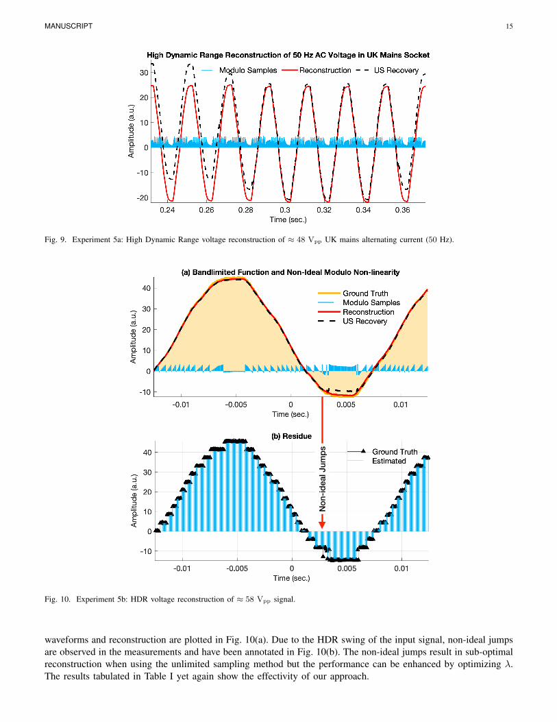
Fig. 9. Experiment 5a: High Dynamic Range voltage reconstruction of ≈ 48 Vpp UK mains alternating current (50 Hz).

Non

-idea

l Jum

ps

Fig. 10. Experiment 5b: HDR voltage reconstruction of ≈ 58 Vpp signal.

waveforms and reconstruction are plotted in Fig. 10(a). Due to the HDR swing of the input signal, non-ideal jumpsare observed in the measurements and have been annotated in Fig. 10(b). The non-ideal jumps result in sub-optimalreconstruction when using the unlimited sampling method but the performance can be enhanced by optimizing λ.The results tabulated in Table I yet again show the effectivity of our approach.

MANUSCRIPT 16

IV. CONCLUSIONS AND TAKE-HOME MESSAGE

In our previous works on unlimited sampling [1]–[3], we studied new acquisition protocols and recoveryalgorithms for high-dynamic-range sensing based on modulo measurements. In this paper, we revisited this problemand proposed a novel solution approach, which, in contrast to the first works, is robust to non-idealities, as weobserved them in experiments with a hardware prototype that we developed.

Our new algorithm is designed for finite-dimensional, folded signals and is agnostic to the sensing threshold λ.The main insight behind our approach is that the folds introduced by the modulo non-linearities can be isolated inthe Fourier domain, which gives rise to a frequency estimation problem. For recovery, we rely on high resolutionspectral estimation methods. This allows us to deal with arbitrarily close folding instants. At the cross-roads oftheory and practice, our work raises interesting questions for future research.• We currently assume that the number of folds is known. We find it very interesting to explore whether this

number can be bounded in terms of function parameters such as the amplitude. Alternatively, developing a robustcriterion for estimating the same from data would benefit the recovery procedure.

• Although we have presented empirical results based on experiments with a hardware prototype, our analysisdoes not yet consider the case of noise for the Fourier domain approach. This remains an interesting pursuit tocomplement our guarantees.

• At the core of the recovery procedure designed in this paper is a spectral estimation problem [28]. We expectthat future advances for this problem will also have interesting implications for the problem of reconstructionfrom modulo measurements. In particular, the limitations of current approaches for this problem in terms of thenumber of spikes that can be recovered will also directly translate into limitations of the approach presented inthis paper. Also viewing the problem from the perspective of super-resolution [29] may yield additional insightsand solution strategies.

• As an alternative way to overcome these limitations, in future work we aim to investigate hybrid methods that usethe Fourier domain approach only for spikes that correspond to non-idealities and combine it with the originalunlimited sampling method for the other spikes.

REFERENCES

[1] A. Bhandari, F. Krahmer, and R. Raskar, “On unlimited sampling,” in International Conference on Sampling Theory and Applications(SampTA), Jul. 2017.

[2] ——, “Methods and apparatus for modulo sampling and recovery,” US Patent US10 651 865B2, May, 2020.[3] ——, “On unlimited sampling and reconstruction,” IEEE Trans. Sig. Proc. (IEEE Xplore Early Access, arXiv:1905.03901), Dec. 2020.[4] ——, “Unlimited sampling of sparse sinusoidal mixtures,” in IEEE Intl. Sym. on Information Theory (ISIT), Jun. 2018.[5] ——, “Unlimited sampling of sparse signals,” in IEEE Intl. Conf. on Acoustics, Speech and Signal Processing (ICASSP), Apr. 2018.[6] R. Rieger and Y.-Y. Pan, “A high-gain acquisition system with very large input range,” IEEE Trans. Circuits Syst. I, vol. 56, no. 9, pp.

1921–1929, Sep. 2009.[7] K. Itoh, “Analysis of the phase unwrapping algorithm,” Applied Optics, vol. 21, no. 14, pp. 2470–2470, Jul. 1982.[8] A. Bhandari and F. Krahmer, “HDR imaging from quantization noise,” in IEEE Intl. Conf. on Image Processing (ICIP), Oct. 2020, pp.

101–105.[9] A. Bhandari, M. Beckmann, and F. Krahmer, “The Modulo Radon Transform and its inversion,” in European Sig. Proc. Conf.

(EUSIPCO), Oct. 2020, pp. 770–774.[10] M. Beckmann, F. Krahmer, and A. Bhandari, “HDR tomography via modulo Radon transform,” in IEEE Intl. Conf. on Image Processing

(ICIP), Oct. 2020, pp. 3025–3029.[11] S. Fernandez-Menduina, F. Krahmer, G. Leus, and A. Bhandari, “DoA estimation via unlimited sensing,” in European Sig. Proc. Conf.

(EUSIPCO), Oct. 2020, pp. 1866–1870.[12] ——, “Computational array signal processing via modulo non-linearities,” IEEE Trans. Sig. Proc. (under submission), Aug. 2020.[13] O. Ordentlich, G. Tabak, P. K. Hanumolu, A. C. Singer, and G. W. Wornell, “A modulo-based architecture for analog-to-digital

conversion,” IEEE J. Sel. Topics Signal Process., pp. 1–1, 2018.[14] A. Bhandari and F. Krahmer, “On identifiability in unlimited sampling,” in Intl. Conf. on Sampling Theory and Applications (SampTA),

Jul. 2019.[15] E. Romanov and O. Ordentlich, “Above the Nyquist rate, modulo folding does not hurt,” IEEE Signal Process. Lett., vol. 26, no. 8,

pp. 1167–1171, Aug. 2019.[16] O. Musa, P. Jung, and N. Goertz, “Generalized approximate message passing for unlimited sampling of sparse signals,” in IEEE Global

Conf. on Signal and Information Proc. (GlobalSIP), Nov. 2018.[17] O. Graf, A. Bhandari, and F. Krahmer, “One-bit unlimited sampling,” in IEEE Intl. Conf. on Acoustics, Speech and Signal Processing

(ICASSP), May 2019, pp. 5102–5106.[18] L. Gan and H. Liu, “High dynamic range sensing using multi-channel modulo samplers,” in IEEE Sensor Array and Multichannel Sig.

Proc. Workshop (SAM), Jun. 2020.

MANUSCRIPT 17

[19] S. Rudresh, A. Adiga, B. A. Shenoy, and C. S. Seelamantula, “Wavelet-based reconstruction for unlimited sampling,” in IEEE Intl.Conf. on Acoustics, Speech and Sig. Proc. (ICASSP), Apr. 2018.

[20] M. Cucuringu and H. Tyagi, “On denoising modulo 1 samples of a function,” in Proc. of the 21st Intl. Conf. on Artificial Intell. andStats., ser. Proc. of MLR, vol. 84. PMLR, Apr. 2018, pp. 1868–1876.

[21] V. Bouis, F. Krahmer, and A. Bhandari, “Multidimensional unlimited sampling: A geometrical perspective,” in European Sig. Proc.Conf. (EUSIPCO), Oct. 2020, pp. 2314–2318.

[22] S. Kay, Modern Spectral Estimation, Theory and Application. Prentice Hall Englewood Cliffs, 1988.[23] J. Wolf, “Redundancy, the discrete Fourier transform, and impulse noise cancellation,” IEEE Trans. Commun., vol. 31, no. 3, pp.

458–461, Mar. 1983.[24] O. Rioul, “A spectral algorithm for removing salt and pepper from images,” in 1996 IEEE Digital Signal Proc. Workshop, Sep. 1996.[25] P. Marziliano, M. Vetterli, and T. Blu, “Sampling and exact reconstruction of bandlimited signals with additive shot noise,” IEEE Trans.

Inf. Theory, vol. 52, no. 5, pp. 2230–2233, May 2006.[26] A. Bhandari, Y. Eldar, and R. Raskar, “Super-resolution in phase space,” in IEEE Intl. Conf. on Acoustics, Speech and Signal

Processing (ICASSP), Apr. 2015.[27] Z. Yang, L. Xie, and P. Stoica, “Vandermonde decomposition of multilevel Toeplitz matrices with application to multidimensional

super-resolution,” IEEE Trans. Inf. Theory, vol. 62, no. 6, pp. 3685–3701, Jun. 2016.[28] Y. Hua and T. K. Sarkar, “Matrix pencil method for estimating parameters of exponentially damped/undamped sinusoids in noise,”

IEEE Trans. Acoust., Speech, Signal Process., vol. 38, no. 5, pp. 814–824, May 1990.[29] D. L. Donoho, “Superresolution via sparsity constraints,” SIAM Journal on Mathematical Analysis, vol. 23, no. 5, pp. 1309–1331, Sep.

1992.