Manipulating, Drawing and Entangling Qubits

Marco B. Enrıquezjoint with Oscar Rosas-Ortiz

Chaos i Informacja Kwantowa

January 20, 2014

Department of PhysicsCenter for Research and Advanced Studies, Mexico

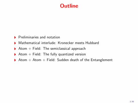
Outline

Preliminaries and notation

Mathematical interlude: Kronecker meets Hubbard

Atom + Field: The semiclassical approach

Atom + Field: The fully quantized version

Atom + Atom + Field: Sudden death of the Entanglement

2/30

Qubits

A two-level atom: Upper level: |+〉 = |e1〉 =

(1

0

), Ground level:

|−〉 = |e2〉 =

(0

1

).

The Hamiltonian: H = ~ωa2σ3. Where ωa is the tansition frequency.

Hilbert space: Ha = span|e1〉, |e2〉.Any state is written as a linear combination:

|ψ〉 = c1|e1〉+ c2|e2〉, ci ∈ C.

The dynamics

σ+ =(

0 10 0

), σ− =

(0 01 0

), σ3 =

(1 00 −1

). (1)

su(2) algebra: [σ3, σ±] = 2σ± and [σ+, σ−] = σ3.

Pauli matrices σ1 = σ+ + σ−, σ− = i(σ− − σ+).

3/30

The Bloch ball and the qubits

Density matrix of a qubit

ρa =( ρ11 ρ12

ρ21 ρ22

)é Normalized: trρa = ρ11 + ρ22 = 1.

é Hermitian: ρ11, ρ22 ∈ R and ρ12 = ρ21.

é Positive: |ρ12| = |ρ21| ≤√ρ11ρ22.

é In the Pauli matrices basis:

ρa =1

2(I + ~τ · ~σ), ~σ = (σ1, σ2, σ3). (2)

4/30

The Bloch ball and the qubits

Where

τ1 = ρ12 + ρ21, τ2 = i(ρ12 − ρ21), τ3 = ρ11 − ρ22.

Since ρa describes a pure or a mixed state: trρ2a = τ21 + τ22 + τ23 ≤ 1.

Equality holds for pure states. Surface of the sphere: S2.

Mixed states within the ball.

5/30

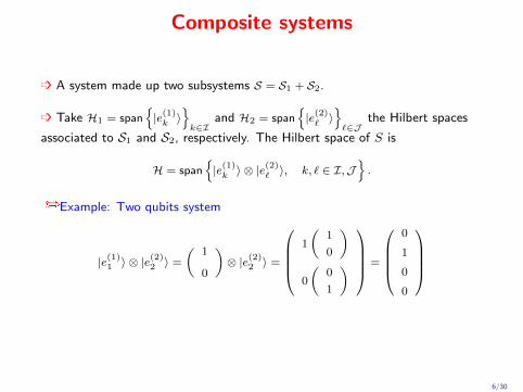
Composite systems

é A system made up two subsystems S = S1 + S2.

é Take H1 = span|e(1)k 〉

k∈I

and H2 = span|e(2)` 〉

`∈J

the Hilbert spaces

associated to S1 and S2, respectively. The Hilbert space of S is

H = span|e(1)k 〉 ⊗ |e

(2)` 〉, k, ` ∈ I,J

.

Example: Two qubits system

|e(1)1 〉 ⊗ |e(2)2 〉 =

(1

0

)⊗ |e(2)2 〉 =

1

(1

0

)0

(0

1

) =

0

1

0

0

6/30

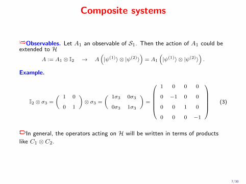
Composite systems

Observables. Let A1 an observable of S1. Then the action of A1 could beextended to H

A := A1 ⊗ I2 → A(|ψ(1)〉 ⊗ |ψ(2)〉

)= A1

(|ψ(1)〉 ⊗ |ψ(2)〉

).

Example.

I2 ⊗ σ3 =

(1 0

0 1

)⊗ σ3 =

(1σ3 0σ3

0σ3 1σ3

)=

1 0 0 0

0 −1 0 0

0 0 1 0

0 0 0 −1

(3)

In general, the operators acting on H will be written in terms of products

like C1 ⊗ C2.

7/30

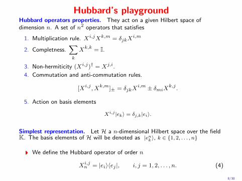
Hubbard’s playgroundHubbard operators properties. They act on a given Hilbert space ofdimension n. A set of n2 operators that satisfies

1. Multiplication rule. Xi,jXk,m = δjkXi,m

2. Completness.∑k

Xk,k = I.

3. Non-hermiticity (Xi,j)† = Xj,i.

4. Commutation and anti-commutation rules.

[Xi,j , Xk,m]± = δjkXi,m ± δmiXk,j .

5. Action on basis elements

Xi,j |ek〉 = δj,k|ei〉.

Simplest representation. Let H a n-dimensional Hilbert space over the fieldK. The basis elements of H will be denoted as |enk 〉, k ∈ 1, 2, . . . , n

We define the Hubbard operator of order n

Xi,jn = |ei〉〈ej |, i, j = 1, 2, . . . , n. (4)

8/30

Hubbard’s playground

Since Hubbard operators are complete, any operator A can be written as follows

A =∑i,j

ai,jXi,jn , ai,j ∈ K, (5)

Example. a 0 0 0

0 b c 0

0 c d 00 0 0 e

0 0 0 −1

0 0 1 00 1 0 0−1 0 0 0

= ?

Deal it with Hubbard!(aX1,1 + bX2,2 + cX2,3 + cX3,2 + dX3,3 + eX4,4

) (−X1,4 +X2,3 +X3,2 −X4,1

)= −aX4,1 + bX2,3 + cX2,2 + cX3,3 + dX3,2 − eX4,1

9/30

Kronecker product highlights

Proposition K1. Let Xi,jm and Xk,`

n be two Hubbard operators of order n

and m respectively. The Kronecker product Xi,jm ⊗Xk,`

n is the mn-Hubbard

operator Xn(i−1)+k,n(j−1)+`mn . That is,

Xi,jm ⊗Xk,`

n = Xn(i−1)+k,n(j−1)+`mn . (6)

Theorem M1. The Kronecker product of A = [ai,j ] and B = [bk,`],respectively n and m-square matrices, can be written as

A⊗B =

nm∑p,q=1

cp,qXp,qnm ≡ C, cp,q := ap′,q′bp′′,q′′

where x′ =⌈xm

⌉and x′′ = x+m−mx′

M. Enrıquez and O. Rosas-Ortiz, “The Kronecker product in terms of Hubbard

operators and the Clebsch-Gordan decomposition of SU(2)× SU(2)”, Annals

of Physics, 339 (2013) 218

10/30

Some applications

Permutation matrices: Let π a bijection of the set of natural numbersS = 1, . . . , n onto itself

π =(

1 2 · · · nπ(1) π(2) · · · π(n)

).

The corresponding permutation matrix in terms of Hubbard operators reads

Pπ =

n∑j=1

Xj,π(j)n . (7)

SU(2) irreducible representation: Let j be a integer or semi-integer

J3 =

n∑k=1

mkXk,kn , n = 2j + 1.

J+ =

n−1∑k=1

√k(2j + 1− k)Xk,k+1

n , J− =

n−1∑k=1

√k(2j + 1− k)Xk+1,k

n .

11/30

Some applications

Haddamard matrix:

H =1√

2

2∑i,j=1

(−1)(i−1)(j−1)Xi,j2 =

1√

2

(1 11 −1

), (8)

Note

H⊗k+1 =1

√2k+1

2k+1∑p,q=1

(−1)~p·~q Xp,q

2k+1 , k ≥ 1, (9)

with

~p · ~q :=

k∑s=0

(ps − 1)(qs − 1), with xs =⌈ x

2s

⌉. (10)

It can be shown that

~p · ~q =

k∑s=0

(p− 1)s(q − 1)s,

where (p− 1)s and (q − 1)s are the s-th binary coefficients of p− 1 and q − 1

respectively.

12/30

Qubit + Classical Field

Qubit Hamiltonian: H0 = ωa2 σ3

Field: E(t) = E(e−iωf t + eiωf t)ef

Interaction Hamiltonian: HI = −p ·E(t), where p = p(σ+ + σ−)ep isthe dipole operator of the atom

Moving to the rotating frame we have

H =∆

2σ3 + g(σ+ + σ−), g = pEep · ef , ∆ = 1−

ωfωa. (11)

In terms of X-operators

H =∆

2

2∑p=1

Xp,p2 + g

2∑p=1

Xp,3−p2 (12)

13/30

Qubit + Classical Field

The time evolution operator in terms of X-operators

U(t) =

2∑p,q=1

up,q(t)Xp,q2 +

i∆

2Ω

2∑p=1

(−1)pXp,3−p2 , Ω =

√Ω2/4 + g2

and the coefficients

up,q(t) =( g

Ω

)|p−q|ei π2|p−q|

cos(

Ωt−π

2|p− q|

).

Suppose the initial state is given by |ψ(0)〉 = |ek〉 with k = 1, 2. Thus

|ψ(t)〉 = U(t)|ek〉 =

2∑p=1

up,k(t)|ep〉+i∆

2Ω(−1)k+1|e3−k〉.

Any operator can be written in terms of Hubbards

σ3 =

2∑`=1

(−1)`+1X`,`2 ,

14/30

Qubit + Classical Field

Then the atomic population inversion reads

〈σ(t)〉 = (−1)k+1

[( gΩ

)2cos(2Ωt) +

(∆

2Ω

)2]. (13)

Figure: Atomic population inversion for: k = 1 the initial state is |+〉 and ∆ = 0

(black), ∆ = g (red) and ∆ = 4g (blue).

15/30

Qubit + Classical FieldThe correspondent density matrix reads

ρ(t) =∑p,q

up,kuq,kXp,q2 +

(∆

2Ω

)2

|e3−k〉〈e3−k|+

(i∆

Ω(−1)

k∑p

up,kXp,3−p

)sim

.

Figure: Bloch vectors trajectories on S2. The initial state is |+〉 and ∆ = 0 (black),

∆ = g (red) and ∆ = 4g (blue).

16/30

Qubit + Quantized Radiation Field

Electric field: E(t) = E(e−iωta+ eiωta†)

In the RWA

H =

H0︷ ︸︸ ︷ωfa†a+

ωf

2+ωa

2σ3

+ g(σ+a+ σ−a†)︸ ︷︷ ︸

HI

We will suppose ∆ = 0, (ωf = ωa)

Such a Hamiltonian acts on states like

|e1〉n := |+, n〉, |e2〉n = |−, n+ 1〉,

17/30

Qubit + Quantized Radiation Field

The following set of 4 operators is a representation of the Hubbard operatorsof order 2

X1,1 =

( I 0

0 0

), X1,2 =

(0

∑n

|n〉〈n+ 1|

0 0

),

X2,1 =

(0 0∑

n

|n+ 1〉〈n| 0

), X2,2 =

(0 0

0 I

) (14)

The Hamiltonian is written as

H0 = (N + 1)X1,1 +NX2,2, HI = γ

2∑p=1

Np Xp,3−p, Np =

√N + 2− p

The time evolution operator reads

U(t) =

2∑p,q=1

up,q(Np) Xp,q , up,q(Np) = eiπ2|p−q| cos

(γtNp −

π

2|p− q|

).

18/30

Qubit + Quantized Radiation Field

In general, a initial state could be written as a linear combination of basiselements |e1〉n, |e2〉n for any n

|ψ(0)〉 =

2∑i=1

∞∑m=0

Qim|ei〉m,∑i

∑m

|Qim|2 = 1

Hence|ψ(t)〉 =

∑p,q

∑n

Qqn up,q (gn) |ep〉n. (15)

For instance

Taking Qin = δi,kδm,n then |ψ(0)〉 = |ek〉n. The atomic populationinvertion

σ3(t) = (−1)k+1 cos [2gnt] , gn = γ√n+ 1.

The state |ψ(0)〉 =∑n αn|ek〉n is obtained by Qin = δi,2 αn. The atomic

population invertion

σ3(t) = (−1)k+12∑p=1

∑n=0

|αn|2(−1)p+1|up,2(gn)|2 = (−1)k+1∑n=0

|αn|2 cos(2gnt).

19/30

Qubit + Quantized Radiation FieldThe quantum analogy of Rabi oscillations

20/30

Qubit + Quantized Radiation Field

The reduced density matrix of the atom

ρat(t) =∑m=0

〈m|ρ(t)|m〉 =∑k,p

ak,pXk,p2 , ak,p =

2∑q,`=1

∑n=0

QqnQ`nup,q(gn)uk,`(gn)

Figure: Left: Atomic population inversion. Right: Trajectories within the Bloch ball.

21/30

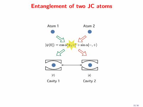
Entanglement of two JC atoms

22/30

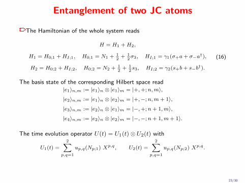
Entanglement of two JC atoms

The Hamiltonian of the whole system reads

H = H1 +H2,

H1 = H0;1 +HI;1, H0;1 = N1 + 12

+ 12σ3, HI;1 = γ1(σ+a+ σ−a†),

H2 = H0;2 +HI;2, H0;2 = N2 + 12

+ 12s3, HI;2 = γ2(s+b+ s−b†).

(16)

The basis state of the corresponding Hilbert space read|e1〉n,m := |e1〉n ⊗ |e1〉m = |+,+;n,m〉,

|e2〉n,m := |e1〉n ⊗ |e2〉m = |+,−;n,m+ 1〉,

|e3〉n,m := |e2〉n ⊗ |e1〉m = |−,+;n+ 1,m〉,

|e4〉n,m := |e2〉n ⊗ |e2〉m = |−,−;n+ 1,m+ 1〉.

The time evolution operator U(t) = U1(t)⊗ U2(t) with

U1(t) =

2∑p,q=1

up,q(Np;1) Xp,q , U2(t) =

2∑p,q=1

up,q(Np;2) Xp,q .

23/30

Entanglement of two JC atoms

Then

U(t) =

4∑p,q=1

up′,q′(Np′;1

)up′′,q′′

(Np′′;2

)Xp,q

4 .

The time evolution of any state

|ψ(t)〉 =∑p,q

∑n,m

Qqn,m wp,k(n,m) |ek〉n,m, wp,k(n,m) = up′,k′ (gn)up′′,k′′ (gm),

The reduced density matrix of the two qubits

ρat(t) =

4∑p,k=1

ap,k Xp,k4 , ap,k =

4∑q,`=1

∑n,m=0

Qqn,mQ`i,j wp,q(n,m)wk,`(i, j).

For instance, suppose the initial state is given by|ψ(0)〉 = (cosα|+,−〉+ sinα|−,+〉)⊗ |r + 1, s+ 1〉. (17)

24/30

Wootters and the ConcurrenceHow much entangled are two systems?

The concurrence C of a bipartite system whose density matrix is ρ, is givenby

C(ρ) = max 0,√λ1 −

√λ2 −

√λ3 −

√λ4,

where λ1, λ2, λ3 and λ4 are the eigenvalues of the matrix ρ(σ2 ⊗ σ2)ρ?(σ2 ⊗ σ2).Here ? means the complex conjugate. Besides, the eigenvalues λi satisfyλ1 ≥ λ2 ≥ λ3 ≥ λ4.

Example. For pure state given as|ϕ〉 = a1|+,+〉+ a2|+,−〉+ a3|−,+〉+ a4|−,−〉, (18)

the concurrence reads C (|ϕ〉〈ϕ|) = 2|a1a4 − a2a3|.

Bell state a1 = a4 = 1√2

. Then C (|ϕ〉〈ϕ|) = 1.

Separable statea1a4 − a2a3 = 0.

Thus C (|ϕ〉〈ϕ|) = 0.

25/30

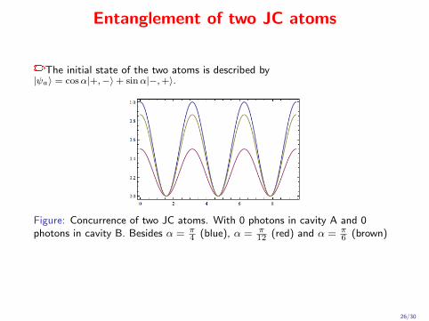
Entanglement of two JC atoms

The initial state of the two atoms is described by|ψa〉 = cosα|+,−〉+ sinα|−,+〉.

Figure: Concurrence of two JC atoms. With 0 photons in cavity A and 0photons in cavity B. Besides α = π

4 (blue), α = π12 (red) and α = π

6 (brown)

26/30

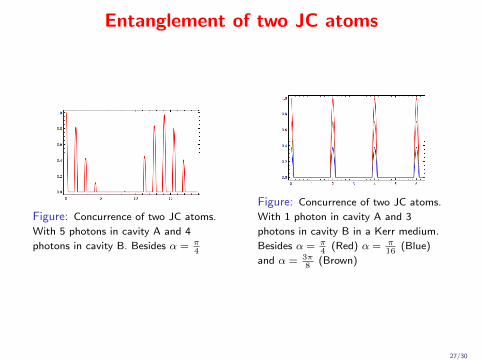
Entanglement of two JC atoms

Figure: Concurrence of two JC atoms.

With 5 photons in cavity A and 4

photons in cavity B. Besides α = π4

Figure: Concurrence of two JC atoms.

With 1 photon in cavity A and 3

photons in cavity B in a Kerr medium.

Besides α = π4

(Red) α = π16

(Blue)

and α = 3π8

(Brown)

27/30

Conclusions

We studied the dynamics of qubits using the Hubbard operators.Interacting qubits?

A geometrical representation of the qubits was given in terms of convexsets. Two qubits?

“Collapses and revivals” of Concurrence of two JC were analized.

Too much work to continue doing!

Thanks!

28/30

The Bar Quantum

QuantumFest 2013You are invited to QuantumFest 2014!!!

29/30

Mexico city and the Cinvestav

30/30