NASA-CR-393719860004808

N ASA r""' ..... 4-_",-.4-""'_ R ...... ~""'-4- 3°3/ 1 I Ii 'UUJ.J.L.I. a\...LU.I. .I. CIJUJ. L 7- / .&.

'\,,-

,(O,r'<

¥for ~ ~ :r4~ noM nns .100M

Magnetic Suspension and Balance System Advanced Study

R.W. Boom, Y. M. Eyssa, G. E. McIntosh, and M. K. Abdelsalam

CONTRACT NASl-17931 OCTOBER 1985

·NI\S/\

r-: .,. JJ 'i'

~~ t~ CUPV

LANGLEY R=:SEJ!,F?CH CENTER L!BR/!.r(';i.> :"'-JASA

_.---_.- ---,- -----

. 111\11111 llll 1111 11111 Illl\ 11111 1'111 tIll 1111 NF02284

https://ntrs.nasa.gov/search.jsp?R=19860004808 2020-05-08T12:12:34+00:00Z

NASA Contractor Report 3937

Magnetic Suspension and Balance System Advanced Study

R. W. Boom, Y. M. Eyssa, G. E. McIntosh, and M. K. Abdelsalam

Madison Magnetics, Inc. Madison, Wisconsin

Prepared for Langley Research Center under Contract NASl-17931

NI\5/\ National Aeronautics and Space Administration

Scientific and Technical Information Branch

1985

FOREWORD

The purpose of this report is to present the results of an advanced study of a Magnetic Suspension and Balance System suitable for a wind tunnel having an 8 ft. x 8 ft. test section capable of operating at speeds up to Mach 0.9 with ±0.1% control forces at 10 Hz for an F-16 model airplane.

R. W. Boom, Y. M. Eyssa, G. E. McIntosh and M. K. Abdelsalam are the major contributors to the study.

Use of trade names or names of manufacturers in this report does not constitute an official endorsement of such products or manufac­turers, either expressed or implied, by the National Aeronautics and Space Administration.

iii

j j j j j j j j j j j j j j j j j j j j j j j

j j j j j j j j j j j

j j j j j j

j j j

j

j j j j

FINAL REPORT ON NASA CONTRACT NASl-17931

"MAGNETIC SUSPENSION AND BALANCE SYSTEM ADVANCED STUDY"

PROJECT SUMMARY

The objectives of this study were to investigate advanced topics in Magnetic Suspension and Balance Systems (MSBS). The advanced topics were identified as potential improvements by Madison Magnetics, Inc. (MMI) during a 1984 study of an MSBS utilizing 14 external superconduc­tive coils and a superconductive solenoid in the airplane test model suspended in a wind tunnel. ~llien substituted in the 1984 MMI design, these improvements result in a selectively new 1985 MSBS design. SpeCifically, the objectives were to investigate test model solenoid options, dynamic force limits on the model, magnet cooling options, structure and cryogenic designs, power supply specifications, and cost and performance evaluations.

All objectives were achieved, as seen in the specification and performance chart, where each entry shows improvement for the 10 Hz ± 0.1% force requirement.

Specifications ======================================================================== MMI Cost System Coil Coil Helium Designs

($106) Weight Weight Conductor Liquefier (tonnes) (tonnes) (MAm) (liters/h)

1984 29.9 368 171 755 560 1985 21. 4 210 80.9 468 375

Performance =======================================================~================

MMI Test Coil Wing AC Loss Control Magnet System Designs Pole Magnet- at 10 Hz Freq. Stored Power

Strength ization to Helium Limit Energy (l04Am) (tesla) (W) (Hz) (MJ) (MW)

1984 3.75 0.70 2212 10 906 97.2 1985 4.45 0.98 522 30 408 31.2

The improvements are due to: magnetic holmium coil forms in the model, better rare earth permanent magnets in the wings, fiberglass-epoxy structure replacing stainless steel, better coil configuration and new saddle roll coil design.

Primary commercial application of the research is for high performance conventional and cryogenic wind tunnels. Secondary commer­cial application to other disciplines is expected for the high current density test model coil and for the low loss AC magnet designs.

v

TABLE OF CONTENTS

Foreword ••••••••• Pro j ec t Sunnnary ....•••••.•....•••.•.....•••...•.•...••...•...•.•. Table of Contents .......................... . Lis t of Figures ................................................. . List of Tables .••••••••••••••.•••••••••••••••••••••••••••••• References ••••.••

1.

II.

III.

Introduction .............................................. . 1.1 1.2 1.3

System 11.1 11.2 II.3 II.4 II.5 II.6

Magnet III. 1

III.2 III.3

Background ......................................... . Summary ••.••• 41 •• e .•••••••.••••••••••••••••••••••••••••

Phase 1.3.1 1. 3. 2

I Accomplishments ............................. . Phase I Phase I 1.3.2.1 1.3.2.2 1.3.2.3 1.3.2.4

1.3.2.5

1.3.2.6

1.3.2.7

1.3.2.8 1.3.2.9 1.3.2.10

1.3.2.11 1.3.2.12 1.3.2.13

Program ........•..•.....••.••..•••••. Obj ectives .......................... . Best Design at 4.2 K •••••••••••••••• Best Design at 1.8 K •••••••••••••••• Best Design for Forced Flow Cooling. Best Structural Design for Minimum AC Losses •••• Best Cryogenic Systems for Various Duty Cycles •• Stable Conductor Designs with Low AC Losses •••• Parameter Variation vs. Control Freque~cy.~ ••••••••••••• Improved Power Supply Specifications Series Connected Coils ••••••••• Solenoid Designs for Suspended Models ....... . ' ..........•. ' ......... . Drag Coils Elimination Study •••••••• Design Summaries and Cost Estimates. Key Items for Phase II Research and Development .. · .................. .

Des ign ....•...................•..•..•............... MSBS System Concepts ............................... . Magnetic Properties of the Model Coil ••••••••••••••• Wing Permanent Magnet Material •••••••••••••••••••• Magnetic Field Requirements ••••••••••••••••••••••• Cross Coupling ..................................... . System Configuration ............................... .

Design ............... ~ ...........•................ Magnet System ....................•......... ........ III. 1. 1 IlL!. 2 IlL!. 3

Co il Shapes •••••••••••••••••••••••••••••••• Coil Terminal Voltages •••••••••••• Magnet Control Requirement.

Conductor .......................... . Magnet System Concept ••••••••••••••• Ill. 3. 1 III. 3. 2 III. 3. 3

System Analysis ...................... . Model Core Solenoid ....................... . x, Y, Z and R Coils .....•.•...•............

vii

iii v

vii ix x

xi

1 1 2 4 4 5 5 5 5

6

6

6

7 7 8

8 8 8

9

11 11 12 17 18 19 21

23 23 23 23 24 25 25 25 29 33

IV.

V.

VI.

VII.

System IV.l IV.2

IV.3

IV.4

IV.5

Analysis ............................................ . Parametric Study ................................... . Conduc tors ......................................... . IV.2.1 IV.2.2 Cooling IV.3.1 IV.3.2 IV.3.3 IV.3.4

Conductor for Pool Boiling •••••••••••••••••• Forced Flow Cooling............... • ••••••• Methods ••.•••••••••••••••••••••••••••••••••• Pool Cooling at 4.2 K ••••••••••••••••••••••• Superfluid Helium at 1.8 K •••••••••••••••••• Forced Flow Cooling ••••••••••••••• Cone Ius ions ...................... .

AC Losses and Control Requirements •••••••••••••••••• IV.4.1 External Magnet Losses and Control

Requirements ............................... . IV.4.2 Model Coil Losses and Control Limits •••••••• Drag Coil Requirements ••.•..•....•........•••••.....

Structural and Thermal Design •••••••••••••••••••••••••••••• V.l V.2 V.3 V.4 V.5 V.6

Structure Concepts ..•••••....••••........••••.•.••.. Materials ..................................... ., .... . Forces and Torques ....••..•..........•....•••......• Structural Design...... ••••••• • •••••••••••••• Electrical Isolation •••••••••••••••••••••••••••••••• Weigh t Summary •..•.......•.••.......•••...•.•....•.•

Thermal and Cryogenic System •.•••••••••••••••••••••••••••.• VIol VIo2 VIo3 VIo4 VIo5 VI. 6 VI. 7 VI. 8 VI. 9

Cryogenic Concepts ................................. . Cryostat Heat Leak ..........••...••..•.•....•... " .•. Magne t Power Leads ..•............................... Operating Component Cryogenic

Losses ••••••.•••••••••••••••••••••••••••• " Review ................................... . System Cost Estimate ••••••••••••••••••••••

Co·oldown Analysis .........•......................... General Operating Plan .••.••...••••••....•••••••.••. Cryogenic Impact of 1.8 K Operation •••••••••••••••••

Cost Estimate ..................................•...•.......

39 39 39 40 47 49 49 49 50 50 51

51 52 54

55 55 59 65 65 67 68

69 69 69 72 72 75 78 78 79 81

83

VIrI. Appendices................................................. 87 A.

B. C. D. E. F.

Appendix A

Appendix B Appendix C Appendix D Appendix E Appendix F

Magnetic Pole Strength of a Superconducting Solenoid with Holmium Mandrel Roll Torque Analysis Forces and Torque Requirements Cross Coupling Analysis Optimizations of Drag and Roll Coils Tunnel Wall Constraints

viii

89 91 95 97

101 III

Figure Figure

11.1 11.2

LIST OF FIGURES

1984 Magnet System ................................. . 13 1985 Magnet System with Saddle Roll Coils

and In-Line Drag Coils........................... 14 Figure 11.3 Dem~gnetization Curve of Nd13.5DY1.4Fe77B8

Sl.ntered Magnet.................................. 18

Figure 111.1 Core Magnet Cryostat............................... 34

Figure IV.l Z or Y Coil Parameters vs. Gross Current Density J. 43 Figure IV.2 Z or Y Coil Outer Radius vs. Magnetic Field........ 44 Figure IV.3 Cryostable 11 kA AC Cable.......................... 45 Figure IV.4 15 kA Forced Flow Conductor........................ 48

Figure V.1 Cryostat Longitudinal Section...................... 56 Figure V.2 Cryostat Transverse Section........................ 57 Figure V.3 Structural Electric Break.......................... 60 Figure V.4 Cold Shell Electrical Break........................ 61 Figure V.5 Egg Crate Electrical Break......................... 62 Figure V.6 End Plate Assembly................................. 63 Figure V.7 Roll Coil Restraint and Structural Stiffener....... 64

Figure VI.1 MSBS Cryogenic Schematic........................... 70

Figure B.1 F16 Wing........................................... 92 Figure B.2 Wing Cross-Sectional Area.......................... 93 Figure E.1 Field Due to Current Sheet......................... 102 Figure E.2 Quadrupole Field of the Roll Coil at the

Model Wing Tip..................................... 104 Figure E.3 Field on the Axis of the X Drag Coils.............. 104

ix

Table II-I Table II-2 Table II-3 Table II-4

Table II-5 Table II-6

Table III-1 Table III-2 Table III-3 Table III-4 Table III-5 Table 1II-6

Table III-7 Table III-8 Table 1II-9 Table III-10 Table III-ll Table III-12 Table III-13 Table IV-1

Table IV-2

Table IV-3

Table IV-4

Table IV-5 Table IV-6 Table IV-7 Table IV-8

Table IV-9

Table IV-10 Table V-I Table VI-1 Table VI-2 Table VI-3 Table VI-4 Table VI-5 Table VII-1

Table C-1 Table F-1

LIST OF TABLES

Madison Magnetics MSBS 1984 and 1985 Designs ••.•••• Holmium Magnetization vs. Applied Field at 4.2 K ••• Model Coil Specifications •••••••••••••••••••••••••• Magneti~ Properties of Nd15Fe77B8 Magnetic

Materlal ........................................ . Field Requirements in Tesla at Model Coil Pole Tips X. Y and Z Coil Fields in Tesla at Zero Angle

of Pitch, Yaw and Roll ....................•...... Voltage and Power Requirements per Coil •••••••••••• Maximum Fields in Coils in Tesla .•••••••••••••••••• Forces and Torques on Z. Y and X Coils ••••••••••••• Forces on the R-Coil •••.•..............•••..•...... Inductance Matrix in Milli-Henries ••••••••••••••••• Forces and Torques on the Drag Coils due to the

Roll Coils ...................................... . Model Coil Parameters .........•.••.•..•.....•...... X Drag Coil Parameters •.......••..••........•...•.. Z or Y Col.l Pa.rameters •.••........•.......•.•.•.... Roll Coil Specifications ••••••••••••••••••••••••••• Coil Weights J kg .................................. . Coil AC Losses at 10Hz .....................•...... Eddy Current Losses in Structure and Helium Vessel. Z Coil Dimensions as Function of Field

and Gross Current Density (J = 1500 A/Cm2 ) •••••••

Z Coil Dimensions as Function of Field and Gross Current Density (J = 2500 A/cm2 ) •••••••

Z Coil Dimensions as Function of Field and Gross Current Density (J = 3500 A/cm2 ) •••••••

Z Coil Dimensions as Function of Field and Gross Current Density (J = 4500 A/cm2 ) •••••••

Characteristics of the ANL Cable Conductor ••••••••• ANL Cable Conductor for 4.2 K and 1.8 K Operation •• JAERI JF-15 Forced Flow Conductor •••••••••••••••••• MSBS Cost Differences for 1.8 K Hell or Forced

Cooling Systems Compared to 4.2 Cooling •••••••••• Maximum Control Variation of Current

vs. Control Frequency ...........•.•....•..•.•.... Model Coil Losses vs. Control Requirements ••••••••• MSBS System Estimated Weights •••••••••••••••••••••• Static Heat Leak and Cryogen Consumption ••••••••••• Predicted Lead Losses .•.••.....•....••..........•.. Magnet and Cryostat Operating Losses ••••••••••••••• Components of MSBS Cryogenic Systems ••••••••••••••• Cryogenic System Cost Estimates •••••••••••••••••••• MSBS Cost Estimate--Control Based on 0.1% I

at 10 Hz in All Coils Simultaneously ••••• ~~~ ••••• MSBS Requirements. 8' x 8' Test Section •••••••••••• Time Constants for Field Diffusion

12 16 16

17 19

20 24 26 26 27 28

29 30 33 35 35 36 37 37

40

41

42

42 45 47 49

51

52 53 68 71 72 73 75 79

85 96

Through Dewar Walls.............................. 112

x

[lJ

[2J

[3J

[4J

[5J

[6]

[7]

[8J

[9J

REFERENCES

H. 1. Bloom et al., "Design Concepts and Cost Studies for Magnetic Suspension and Balance Systems," NASA CR-165917, July 1982.

R. W. Boom, Y. M. Eyssa, G. E. McIntosh, and M. K. Abdelsalam, "Magnetic Suspension and Balance System Study," NASA CR-3802, July 1984.

S. J. Sackett, uEFFI : A Code for Calculating the Electromagnetic Field and Inductance in Coil Systems of Arbitrary Geometry~ Lawrence Livermore Laboratory, Livermore, California, UCRL-52402, March 1978.

V. Takashi et al., "Development of a 30-kA Cable-in-Conduit Conductor for Pulsed Poloidal Coils," IEEE Transaction on Mag­netics, Vol. MAG-19, No.3, May 1983, p. 386.

W. Schauer and F. Arendt, "Field Enhancement in Superconducting Solenoids by Holmium Flux Concentrators," Cryogenics, October 1983.

R. W. Hoard et al., "Field Enhancement of a 12.5 T Magnet Using Holmium Poles," IEEE Transactions on Magnetics, Vol. MAG-21, No.2, March 1985.

M. Sagawa et al., "Permanent Magnet Materials Based on the Rare Earth-Iron-Boron Tetragonal Compounds," iEEE Transactions on Magnetics, Vol. MAG-20, No.5, September 1984.

S. Arai and T. Shibata, "Highly Heat Resistant Nd-Fe-Co-B System Permanent Magnets," paper presented at the 1985 INTERMAG Confer­ence, St. Paul, Minnesota.

S. H. Kim, S. T. Wang. and M. Lieberg, "Operating Characteristics of a 1.5 MJ Pulsed Superconducting Coil," Advances in Cryogenic Engineering, Vol. 25, Plenum Press, N.Y., 1980, pp. 90-97.

xi

j j j j j j j j j j j j j j j j j j j j j j

j j j j j j j j j j j

j j j j j

j j j

j

j j j j

I. I!'-lTRODUCTION

1.1. Background

Magnetic suspension and balance systems (MSBS) for wind tunnels

have been increasingly developed and utilized during the past 25 years.

The primary aerodynamic advantage of MSBS is the elimination of air flow

disturbances caused by the test model mechanical support system and by

the required alterations in the test model. The primary technological

advantages of MSBS are that static and dynamic forces and torques on the

test model can be applied and recorded (from magnet currents) without

the severe sting restraints.

The potential availability of MSBS for large transonic tunnels

improves steadily in line with the expanding broad utilization of

superconductive magnet systems in many fields, such as: magnetic

resonance imaging, high energy physics, fusion, and energy storage.

Superconductive systems are needed because the external magnets are far

from the test model and, in some cases, tend to cancel fields from other

magnets.

The recent conceptual design studies by General Electric [1) in

1981 and by Madison Magnetics [2J in 1984 show that practical super­

conductive MSBS systems can be built well within the present state of

the art for superconductive systems. Design improvements and cost

reductions continue in this third design study for a MSBS suitable for

an 8' x 8' test section at Mach 0.9 with ±0.1% control forces at 10 Hz

for an F16 model airplane.

1

1. 2. Summary

The cost estimate for this MSBS design is $21,398,000 in 1985

dollars, which is a reduction of 29% from the 1984 Madison Magnetics,

Inc. (MMI) design. The 1984 design was itself a considerable improve­

ment over the 1981 design due, primarily, to the efficient compact

mounting of external magnets in one dewar so as to be as close as

possible to the test airplane model in the wind tunnel.

Some special features of the MMI-1984 design are as follows:

* Superconductive persistent solenoid in the suspended airplane

model instead of magnetized iron.

* Permanent magnet wings instead of magnetized iron wings.

* New race-track roll coils.

The new features of the MMI-1985 design are:

* Magnetic holmium coil forms for the test model superconducting

core solenoid.

* *

*

Better permanent magnet material, Nd15Fe77B8' in the wings.

Saddle roll coils and in-line smaller diameter drag coils.

Fiberglass epoxy structure.

In Chapter II, System Design, the system specifications are given

for both 1984 and 1985 MMI designs. The reduction in ampere-meters for

1985 is about 38%. The properties of the holmium test model winding

core and of the Nd15Fe77B8 magnetic boron rare earth wing material are

given. Field requirements and cross-coupling effects are determined for

optimized coil locations.

In Chapter III, Magnet Design, the specifications for the X, Y, Z

and R coils are given. AC losses are dominated by hysteresis losses at

10 Hz in the NbTi filaments. The structure is mostly large plates of

2

fiberglass-epcx)7 't~Thich have no AC loss. The EFFI code [3] modified by

University of Wisconsin is used to find stored energy and mutual forces

between magnets. Operational possibilities for current (and force)

directions in the coils determine force extremes on the structure, as

described.

In Chapter IV, System Analysis, a detailed comparison is made

between magnets cooled in helium baths at 4.2 K and 1.8 K and cooled by

forced flow supercritical helium above 5.2 K. The 4.2 K bath cooling is

shown to be most economical. The 1.8 K bath cooling option is poten­

tially attractive for intermittent short-run time use, which is not the

operational specification for this study. Forced flow cooling has very

large helium pumping losses and is third choice.

Eliminating both drag coils is shown to be impossible. Operation

with one drag coil is possible but only at the cost of more system

ampere-meters of conductor.

In Chapter V, Structural and Thermal Design, a new fiberglass-epoxy

structure is described. This non-metallic lightweight structure has no

AC losses, which would have eliminated the major loss in the 1984 design.

The common objection to using fiberglass-epoxy is helium leakage which

does not apply here since the epoxy structure is totally immersed inside

the helium bath. Electrical eddy current losses are minimized by

electrical breaks in key metallic structural loops. The overall MSBS

weight, components plus structure, is about 60% that of the 1984 design.

In Chapter VI, Thermal and Cryogenic System, the smaller heat load

of this MSBS design needs a 375 ~/h helium liquefier as compared to 560

t/h in the 1984 design. The cryogenic system cost is reduced by 15%. A

brief discussion of advantages and disadvantages of a 1.8 K system is given.

3

In Chapter VII, Cost Estimate, the MSBS cost estimate is $21,398,000.

Compared to the 1984 design [2], major reductions are achieved in:

1.3.2 (winding machine construction) due to available commercial equip­

ment; 1.3.9 (power supplies) due to smaller magnets; 1.3.12 (support

structure) due to simpler fiberglass-epoxy structure slabs; 1.3.18

(manufacturing checkout) due to simpler system; and all magnet con­

struction (1.3.3, 1.3.4, 1.3.5, 1.3.6 and 1.3.7) due to smaller, simpler

coils.

In Chapter VIII, Appendices, six sections provide background

derivations and calculations for model magnet pole strengths, roll

torques, force requirements, cross coupling, drag and roll coil opti­

mization and tunnel wall thickness constraints.

1.3. Phase I Accomplishments

1.3.1. Phase I Program

The objectives of this Phase I study are to investigate advanced

topics in the design of MSBS with emphasis in the superconductive magnet

design area. Many potential improvements and variations noticed by MMI

during the 1984 design are the advanced topics considered.

The objectives are listed below with short descriptive answers and

with reference to the longer, more detailed discussion in the main

report. We choose to present the sum effect of the improvements as an

integrated new MSBS design, which is in fact our 1984 design with these

improvements. The interaction of changes with the whole MSBS requires a

system design evaluation. Therefore, the result of the study of the

advanced topics is a selectively new 1985 design.

4

1.3.2. Phase I Objectives

1.3.2.1. Best Design at 4.2 K

Open pool cooling in 4.2 K-one atmosphere helium in one large dewar

for all 14 external solenoids and roll coils is the best design and is

the cooling option of this report. Chapter IV, Section IV.2 through

IV2.1.1, Section IV.3.1, and Table IV-6 all support this choice with

cost and performance benefits.

1.3.2.2. Best Design at 1.8 K

Open pool cooling in superfluid helium at 1.8 K-one atmosphere is

the second best choice. Conductor cooling is better than at 4.2 K, the

amount of conductor is $750,000 less, and the added cost of 1.8 K

refrigeration is about $1,500,000. Thus, an 1.B K system is more

expensive by 3.5% of the $21 x 106 system cost. This option is de-

scribed in IV.2.1.2, IV.3.2 and IV.3.4.

In IV.9 a zero cost 1.8 K option is seen to provide several hours

of daily operation, which might be adequate for a tunnel with long model

change times. Several hours is less than the specified 2h at full load

and Bh at 1/4 load per day.

1.3.2.3. Best Design for Forced Flow Cooling

Using one of the best forced flow conductors, the J15 conductor

developed at JAERI in Japan [4J, the optimized design for MSBS is a 15

kA conductor. The helium flow work in all 14 magnets is 1500 W, which

is much larger than the total 918 W at full load at 4.2 K. The added

MSBS system cost increase is only 1.6%. This forced flow option is

considered less stable and is the third choice.

Forced flow cooling is described in IV.2.2, IV.3.3 and IV.3.4.

5

1.3.2.4. Best Structural Design for Minimum AC Losses

Epoxy-fiberglass structural slabs, longitudinal electrical breaks

in the inner and outer cold walls of the cryostat, and radial breaks in

the end plate/drag coil containment assemblies all combine to reduce

full load AC structure losses to 200 W (from 1560 W). This eliminates

the largest previous loss. The breaks utilize sharp triangular ridges

which bite into a Vespel sealing strip. Sections V.1 and V.5 and Figs.

V.3, V.4 and V.5 cover the loss aspects of this structural design.

1.3.2.5. Best Cryogenic Systems for Various Duty Cycles

The specified duty cycle of 2h at full load, 8h at 1/4 load and 14h

at zero load is best met by sizing the refrigeration system for the

average daily load and then meeting the peak load with extra stored

helium for the 4.2 K and forced flow options. For 1.8 K superfluid

cooling the enthalpy of 1.8 K helium raised in temperature to 2.0 K

during peak loads applies the same flywheel averaging effect to the

liquefier size. This "average" size is calculated explicitly in VI. 4

and used in VI.9.

1.3.2.6. Stable Conductor Designs with Low AC Losses

Sections IV.1 through IV.2.1.2 present a comprehensive analysis of

the ANL-11 kA conductor r8J for MSBS stable low loss use in 4.2 K or

1.8 K pool cooling. The conductor, pictured in Fig. IV.3, is subject to

a maximum field change of 0.4 T/s although it can withstand 11 T/s and

remain superconducting. The remaining concern, the AC losses, are

primarily NbTi hysteresis losses which constitute the major cryogenic

loss at full load. The ANL conductor is a completely verified AC pulsed

conductor ideally suited for MSBS use.

6

The forced flow conductor, IV.2.2, is less interesting because of

its smaller stability margin. Total losses including AC losses are less

than the helium pumping losses at low temperature.

1.3.2.7. Parameter Variation vs. Control Frequency

In Section IV.4 it is shown that the product [~If] ~16 for B < max

6T and B < 6 Tis in the 14 external magnets. ± ~I% is the variation in

current in any coil at contrpl frequency f. The model coil limit is

[~If] < 3. Thus the product control frequency times AC force ampli-m~ .

tude can be increased by a factor of 3 from the ± 0.1% force at 10 Hz

without significant losses in either the model coil or the 14 external

coils.

1.3.2.8. Improved Power Supply Specifications

The requirement for dynamic control is ±0.1% of any magnet current

at 10 Hz. Accordingly, the maximum voltage across any MSBS coil is set

to satisfy this requirement. The inductances used to calculate voltages

are the self inductance of each coil, since the inductive mutual cou-

pIing between the different sets of coils is very small. The extra coil

groups (X, Y, Z and R) are accounted for in the values of self induc-

tances used.

TheR coils are the primary source of mutual inductive coupling and

induced voltages V. By operating these coils in series with one power p

supply many unwanted high voltage options are eliminated. Thus the

voltages required are reduced and the total installed power is now 31.2

MW. Smaller coils also contribute to less required power.

7

Section 111.1.2 covers the power supply specifications in detail.

1.3.2.9. Series Connected Coils

As described in the previous section the R coils are connected in

series. All other coils are individually powered for maximum freedom of

control.

1.3.2.10. Solenoid Designs for Suspended Models

The new design feature is the magnetic holmium core which

contributes an 18.7% increase to the model solenoid pole strength (see

Section 111.3.2). This change reduces the size of the X and Z coils by

18.7%.

1.3.2.11. Drag Coils Elimination Study

In IV.5 an analytic proof is presented which shows that one drag

coil is required. The present design of two symmetrical drag coils is

more efficient.

1.3.2.12. DeSign Summaries and Cost Estimates

The cost estimate given in Section VII.1 of $21,398,000 reflects

the smaller magnet system due to a higher pole strength test model

solenoid, the more efficient saddle roll coils, and the new permanent

magnet material Nd15Fe77B8 in the wings. A discussion of the cost logic

is given in Section VII. Costs for checkout and acceptance testing,

position sensors and control systems are taken from NASA CR-165917 for

Case 1, Alternate G [1].

8

Design summaries are:

1. Model coil ••••••••••••••• Table 111-7

2. X drag coil •••••••••••••• Table 111-8

3. Z or Y coil •••••••••••••• Table 111-9

4. Roll coils ••••••••••••••• Table 111-10

5. Coil weights ••••••••••••• Table III-II

6. Cryogenic system ••••••••• Table VI-4

7. Structure •••••••••••••••• Chapter V

1.3.2.13. Key Items for Phase II Research and Development

1. Model coil construction and test of a full-scale dewar and coil

wound on a holmium coil form is the most important task. The current

density should achieve the 30 kA/cm2 used in this design and the coil

should survive 10 Hz mechanical oscillations within the prescribed

angular limits for pitch, yaw and roll. The coil should remain super-

conducting and the helium boil-off rate should be acceptable. This

confirmation research and development would substantiate MSBS system

feasibility.

2. A model coil program for 60 kA/cm2 solenoids should be

initiated. Although this is perceived to be an upper limit for current

density in these conditions, it is felt to be so important that an upper"

limit of J should be established. At 60 kA/cm2 all magnets except roll c

and Y coils could be greatly reduced in size.

3. A model wing of Nd15Fe77BS should be fabricated and tested to

confirm utility and to determine if the 15% stainless steel structure

skin is necessary.

9

4. New MSBS system designs should be continued. The major

advances in this present study were not predicted. The expectation is

that other improvements are possible. Cost reductions are certainly

available in case less stringent duty cycles are acceptable. The

2-hour, ± 0.1% force at 10 Hz requirement determines cryogenic system

and power supply specifications. For a shorter duty cycle the 1.8 K

operation is very attractive (Section VI.9).

10

II. SYSTEM DESIGN

11.1. MSBS System Concepts

The 1984 MSBS [2] design by MMI included design improvements which

reduced the costs to 30% of previous estimates. The major improvements

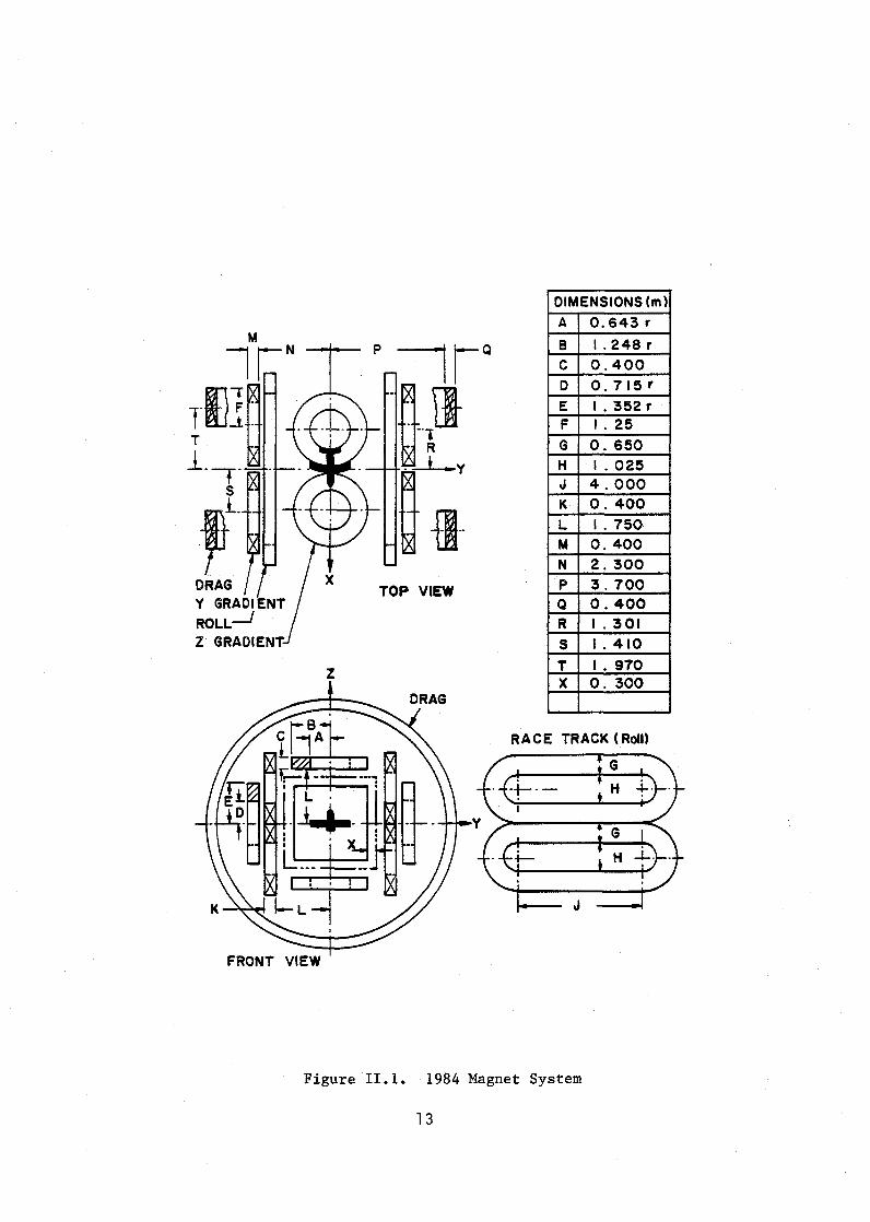
for the 1984 system sketched in Fig. 11.1 are:

* A 70 cm long potted persistent superconducting solenoidal

coil, 11.5 cm c.D., and 6.1 tesla is the model core. A

superconducting coil produces higher magnetic moments and pole

strengths than a magnetized iron core or a permanent magnet

core.

* The model wings contain permanent magnets that occupy 85

percent of the wing volume. The rest of the wing volume is

high strength stainless steel.

* Z and Y gradient coils in Fig. II.l"are symmetric arrays of

four solenoid magnets. They are bipolar coils to control and

manipulate the model. The conductor for all coil systems is

the ll-kA low-loss cryostable conductor.

* The drag coils to counterbalance wind drag forces are large

diameter solenoids.

* The roll coils are four race-track coils optimized for minimum

ampere-meters.

The 1985 MSBS design by MMI adds four additional improvements:

1. The use of a holmium coil mandrel in the suspended model to

increase the core pole tip magnetic moment by 18.7% from 3.75

4 4 x 10 Am to 4.45 x 10 Am.

2. The use of a new permanent magnet material Nd15Fe77B8 in the

11

suspended model wings which reduces the external roll magnet

size by about 25%.

3. The new arrangement for roll and drag coils shown in Fig. 11.2

provides a more economical and compact design.

4. The use of fiberglass-epoxy slabs as the principal structure

to reduce AC losses.

These four improvements reduce significantly the ampere-meters and

energy stored in all 14 external magnets. Table 11-1 compares the two

MM1 designs.

Table II-I

Madison Magnetics MSBS 1984 and 1985 Designs

======================================================================== Coils X Y Z R Total

1984 design Ampere-meters (MAm) 362 100* 86 207 755 Energy stored (MJ) 656 60 50 140 906

1985 design Ampere-meters (MAm) 172 71** 71 154 468 Energy stored (MJ) 216 38 38 116 408

*The Y coils in the 1984 design were undersized due to error in cross coupling relations.

**Actual ampere-meters needed for Y coils are 63 MAm. For sim-plicity of design and to have a complete symmetry, the Y coils are sized the same as the Z coils.

The ampere-meters of conductor in the 1985 design decrease to 62% and

the stored energy decreases to 45% of the 1983 design.

11.2. Magnetic Properties of the Model Coil

The model core solenoid is an epoxy impregnated coil with gross

current density of 30 kA/cm2 at 6.1 tesla maximum fields. Such coils do

12

DIMENSIONS (m)

A 0.643 r M

l rn N

11}1~ 1_+ __ _

S ,L

p l~rQ

n~LI ~~~

x TOP VIEW DRAG

B I_ 248 r C 0.400

D 0_ 715'

E 1.352 r F 1_25

G 0.650 H 1_025 J 4.000 K 0.400

L 1.750· M 0.400

N 2.300

P 3.700 Q 0.400 R 1.301

S 1.410

z T 1.970 X 0_ 300

RACE TRACK (Roln

J

FRONT VIEW

Figure 11.1. 1984 Magnet System

13

..J

I~ p ~I

~M--I ~K All I-B-I

I

'''''' ........... ~ __ ~I ,- ~ kG , i ....",.

----I I" " i

A

LIFT (Z)

" " ROLL (R)

II DRAG (X)

II SI"DE (Y)

- ___ I

...... // .... ......

K >I I~ __ '

Figure II.2. 1985 Magnet system with saddle roll coils and in-line drag coils.

14

Q

-' 1+01 I Y + Z ... .. I II I

VIEW A-A

Figure II.2 (continued)

15

LIFT ROLL

EGG CRATE

SIDE

not contain much copper or cooled surfaces, and their ability to

tolerate disturbances is limited to the adiabatic heat capacity of the

conductor material. However, the absence of large amounts of copper and

helium in the windings allows such coils to operate at current densities

up to ten times as large as those for cryostable coils, which is ideal

for model cores.

The improvement in the present design comes from the holmium

mandrel. Holmium has superior magnetic properties at 4.2 K with a

saturation magnetic moment of 3.9 tesla. Table 11-2 lists the magne-

tization of holmium at 4.2 K [5,6].

Table II-2

Holmium Magnetization vs. Applied Field at 4.2 K

========================================================================

Magnetization force (T) Magnetization (T)

o 0.1 o 1.6

0.52 2.48

1.0 2.9

1.5 2.98

2.5 3.12

3.5 3.25

4.5 3.35

With the specifications shown in Table 11-3, the total magnetic pole

strength of holmium and winding is 4.45 x 104 Am. Appendix A details

6.5 3.7

calculation of the magnetic pole strength as a function of winding and

holmium dimensions.

Table II-3

Model Coil Specifications

======================================================================== ID OD Length Weight Magnetic Pole Strength

(cm) (cm) (em) (k~) (Am)

Winding 8.26 ll.5 70 26.8 3.75 x 104

Mandrel 6.14 8.26 70 14.5 0.70 x lO4

Total 41.3 4.45 x 104

16

Eddy current losses in tb~ model coil are main!}'" hysteresis losses

in the superconductor filaments. For two micron filaments. the expected

hysteresis loss is 0.046 watt (4.6 x 10-3 J/cycle) with ± 0.1% field

variation at 10 Hz for all X. Y. Z and roll coils at full current. The

holmium mandrel resistivity of 3 x 10-S nm at 4.2 K results in eddy

-4 current losses of about 6.4 x 10 watts under the same 10 Hz current

control conditions or two orders of magnitude less than the supercon-

ductor hysteresis loss.

11.3. Wing Permanent Magnet Material

A new superior permanent magnet material Nd1SFe77BS is planned for

the wings [7.S]. The magnetic properties are listed in Table 1I-4.

Table II-4

Magnetic Properties of Nd1SFe77B8 Magnetic Material

======================================================================== Br Hc (BH) max Tc

(T) (kA/m) (kJ/m3) (K)

Nd lS Fe77

B8 1.23 960 290 585

Nd1S(FeO.9CoO.1)77BS 1. 23 800 290 671

Nd1S(FeO.8CoO.2)77B8 1.21 820 260 740

As shown in Fig. II-3. the new permanent magnet material has large

values of M (residual magnetism) and H (demagnetization critical r c

field) • M stays well above 1.2 tesla for most of the demagnetizing r

field and well over 1.lS up to H = 9.60 kA/m (1.21 tesla). With M = c . r

1.lS tesla and 8S% wing volume. the average magnetization in the wing is

0.977S tesla. The required applied Bz field from the roll coil at the

17

tip of the wings at zero angle of roll is B 0.235 tesla compared to z

0.308 tesla used in the previous design (pp. 111-14 of Ref. 2), which is

based on average magnetization of 0.7 tesla using SmCo5

permanent magnet

material. Elimination of the stainless steel skin support in the wing

increases the permanent magnet wing volume to 100% and the average

magnetization to 1.12 tesla. This reduces the B roll field to 0.205 z

tesla and reduces the roll field Am by 12.7%. Mathematical relations

between the roll field required at the wing tips and the average

magnetization are in Appendix B.

NdI3.5DYI.5Fe778a Ndl5Fe77Ba "..... I~ 11.2

0.8 RESIDUAL MAGNETIZATION,

!0.4 M (T)

II I I '0 -1600 -1200 -800 -400 0

DEMAGNETIZING FIELD H (kA/m)

Figure 11.3. D~magnetization curve of NdI3.5DYl.5Fe77B8 slntered magnet [5].

11.4. Magnetic Field Requirements

Maximum external field requirements at the model pole tips during

maximum pitch and yaw are listed in Table 11-5 for the above

18

improvements in model and wing magnetic material. These fields

determine the size of the 14 external magnets. Appendix C lists the

force and torque requirements and their relation to the external

magnets' field.

Table II-5

Field Requirements* in Tesla at Model Coil Pole Tips

========================================================================

Field component*

Field location**

Field required to produce force

Lift

B z

a = 30° 8 10°

0.110

Field required 0.0155 to produce torque

Total field

Margin for control

Total field required

0.1255

2%

0.128

Lateral

B Y

a = 30° 8 = 10°

0.0155

0.0045

0.02

2%

0.0205

Roll Drag (15% SS in Wings) No SS

B x

a 30° 8 = 10°

0.0469

0.0469

2%

0.048

BZR

cjJ = 0 zero roll

0.235

0.235

2%

0.24

0.205

0.205

2%

0.208

*Fields B , B ,B and BZR are fields required to produce maximum x y z

forces and torques at maximum angles of pitch, yaw and roll. These fields are produced by all four coil systems collectively.

**a is the pitch angle, 8 is the yaw angle, and cjJ is the roll angle.

11.5. Cross Coupling

The discussion detailed in Appendix D covers all first order cross

couplings between X, Y, Z, and R coils during pitching, yawing, and

rolling. There were some mistakes regarding signs in some of the

19

equations and the cross-coupling matrix (e.g., Equations 111.9 and

111.10) in Ref. 2. The correct equations and matrix are:

Equation II.1

B = (cos a cos 8) B - (sin 8) B - (sin a) B x Xo YO Zo

B = (1/2 sin 8) B + (cos a cos 8) B + (0) B - A sin a y Xo YO Zo

B = (1/2 sin a) B + (0) B + cos a cos a B - A sin 8 Z Xo YO Zo

cos a cos 8 - sin B

sin 8 cos a cos a ---2

Equation II. 2

- sin a

o

B Xo

B YO

=

B x

B + A sin a Y

sin a 2

o cos a cos 8 B . Zo I

B + A sin B z

J ...

A = (roll coil field, BZR)x L/2b where L is the core length and 2b is

the wing span. B ,B ,and B are the X, Y, Z coil fields at Xo YO Zo

zero angles of pitch and yaw. The maximum design fields of

B ,B , and B are listed in Table 11.6. Xo YO Zo

Table II-6

X, Y, and Z Coil Fields in Tesla at Zero Angle of Pitch, Yaw and Roll

========================================================================

Case I (8.S.reinforced wing)

Case II (no S.S.)

B Xo

0.1664

0.1602

20

B YO

0.1275

0.1099

B Zo

0.1435

0.1390

BZR

0.240

0.204

11.6. System Configuration

The magnet system configuration for the 8' x 8' test section

presented here (Fig. 11.2), is similar to that presented in Ref. 2

(Fig. 11.1), except for:

1. The model core has a holmium mandrel.

2. The four flat race track roll coils in Fig. 11.1 are replaced by

four saddle coils connected in series as shown in Fig. 11-2. The

new configuration reduces significantly the R coil ampere-meters

required to produce a roll field of 0.24 tesla at the wing tips.

3. The two X (drag) coils are placed more in line with the Z and Y

coil systems as shown to simplify the structure required to take

the coupling forces between coils. This arrangement requires

slightly more ampere-meters in the X coils compared to the optimum

position around the four R, Y, and Z coils. However, the present

arrangement simplifies the cryostat and structure design. Optimi­

zation of the drag (X), and roll (R) coil arrangement is detailed

in Appendix E.

21

III. MAGNET DESIGN

111.1. Magnet System Requirement

The magnet system consists of one epoxy impregnated superconducting

model coil with holmium mandrel, 4 Z gradient coils, 4 Y gradient coils,

2 X drag coils, and 4 R roll saddle coils. The Z, Y, and R coils are

fully bipolar while the X coils are monopolar. The symmetry of the coil

array enhances the reliability of the magnet system.

III. L Magnet System Requirement

All system requirements for static forces and torques plus the

10 Hz dynamic control forces are met with the system configuration de­

scribed in Chapter II. Other magnet requirements such as peak magnetic

field strength, peak voltage at the magnet terminals and the structure

requirements are within the state of the art.

111.1.1. Coil Shapes

All coils are solenoids except the saddle R coils. The use of

saddle R coils instead of race track R coils or solenoids minimizes

ampere-meters and stored energy.

111.1.2. Coil Terminal Voltages

The requirement for dynamic control is ± 0.1% of any magnet current

at 10 Hz. Accordingly the maximum voltage across any single MSBS coil

is about 830 V on the X coil.

The power supply maximum voltage and power is determined for I = 11

kA in all coils and for the 10 Hz correction to be applied to each coil

23

continuously at maximim amplitude. The requirements on power supplies

for initial charging to full current in all coils is less than for the

10 Hz load providing the charge time exceeds 25 sec. The 2 min charging

powers are smaller, as seen in Table III-I.

Table III-1

Voltage and Power Requirements per Coil

======================================================================== 10 Hz at 0.1% of 2 min charge

max current sEecification Coil Voltage Power Voltage Power

V MW V MW

Z 76 0.84 16.0 0.18 Y 76 0.84 16.0 0.18 X 830 9.13 174.3 1.92 R* 840 9.23 176.4 1. 94

Total Power** 31. 2 MW 7.22 MW *The four saddle coils used for roll are operated in series and are

considered as one coil. **For all coils simultaneously.

111.1.3. Magnet Control Requirement

The control requirement is ± 0.1% of the stati.c forces at 10 Hz.

Each R, Y and Z magnet has a 3-phase Graetz bridge SCR bipolar power

supply with voltages sufficient to provide the 10 Hz current variation

for control (see Table III-I). The X coils are monopolar and require

only monopolar power supplies. In all cases the power supply voltage

must be sufficient to overcome any unwanted voltage pickup from any

other coil undergoing control current correction in addition to provid-

ing its own dI/dt.

24

111.2. Conductor

The conductor used in all X, Y, Z and R coils is the A1~ 11 kA

cable conductor discussed in Chapter IV.

111.3. Magnet System Concept

The magnet system configuration is shown in Fig. 11.2. The system

consists of 14 superconducting coils arranged around the tunnel test

section. The function and arrangement of these coils is discussed in

Chapter II. All the coil forms are slotted stainless steel with epoxy

plate reinforcement. The forces and torques between the coils are

contained by cold non-metallic structure to minimize eddy current

losses. Details of the dewar and structure are in Chapters V and VI.

111.3.1. System Analysis

The computer code EFFI is used to calculate magnetic fields,

forces, torques, field profiles in the tunnel area, and coil induc­

tances.

The maximum field in each coil is found by field scanning the coil

with operationally paired coils powered to ± 11 kA. The maximum values

for self and total fields are listed in Table 111-2. It is seen that

5.02 T on the Y and Z coils is maximum.

The homogeneity of the magnetic fields in the model region is

examined in detail. Cross coupling between the different coils at

different modes of operation is accounted for, as explained in Chapter

II.

25

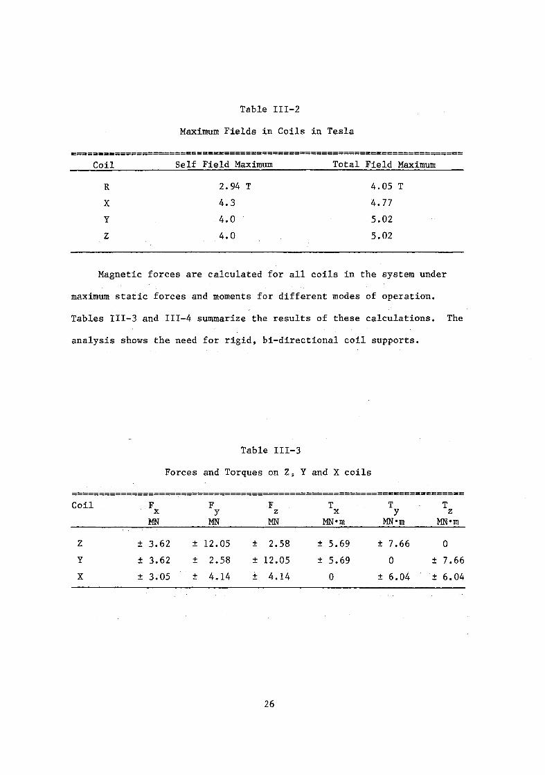
Table 1II-2

Maximum Fields in Coils in Tesla

======================================================================== Coil Self Field Maximum Total Field Maximum

R 2.94 T 4.05 T

X 4.3 4.77

Y 4.0 5.02

Z 4.0 5.02

Magnetic forces are calculated for all coils in the system under

maximum static forces and moments for different modes of operation.

Tables 111-3 and 111-4 summarize the results of these calculations. The

analysis shows the need for rigid, hi-directional coil supports.

Table III-3

Forces and Torques on Z. Y and X coils

======================================================================== Coil F F F T T T

x Y z x Y z MN MN MN MNom MNom MNom

Z ± 3.62 ± 12.05 ± 2.58 ± 5.69 ± 7.66 0

Y ± 3.62 ± 2.58 ± 12.05 ± 5.69 0 ± 7.66

X ± 3.05 ± 4.14 ± 4.14 0 ± 6.04 ± 6.04

26

Table 1II-4

Forces on the R-Coil (half of the top left coil)

======================================================================== Section Type Axis Length F F F x Y z

MN MN MN

1 Straight x-axis 0.7 m 0 ± 1.14 ± 6.25 2 Straight x-axis 0.7 m 0 ± 0.98 ± 4.23 3 Straight x-axis 0.7 m 0 ± 0.98 ± 4.23 4 Straight x-axis 0.7 m 0 ± 1.14 ± 6.25

5 Arc y-axis 90° ± 4.93 ± 2.00 ± 6.15 6 Arc x-axis 90° ± 9.97 ± 1.94 ± 1.43 7 Arc z-axis 90° ± 1.97 ± 2.27 ± 4.43

The self and mutual inductances of the MSBS coil system are calcu-

lated with the computer program EFFI. The inductance matrix is shown in

Table 111-5. The mutual inductances between coils are relatively small

compared to self inductances.

A study of the operational effect on the maximum field, force and

inductance are carried out. To illustrate the outcome of this study we

take one of the drag coils as an example. The forces on this coil due

to each of the four roll coils in the system are shown in Table 111-6.

A study of this table reveals that the maximum force in the x-direction

on the drag coil from the roll coils alone is 43.64 MN. However, to

produce this force, the current in two of the roll coils has to flow in

an opposite direction to the current in the other two R coils. This is

not realistic, because in all modes of operation, the current in each of

the roll coils will be equal and in the same direction since the four

roll coils operate in series. Thus these large forces cancel each

other. A similar situation, but on a smaller scale, occurs for the

drag, Z and Y coils. Every coaxial pair of these magnets will carry

27

Table III-5

Inductance Matrix in Milli Henries

==================================================================================================== Coil Z-1 Z-2 Z-3 Z-4 Y-l Y-2 Y-3 Y-4 X-I X-2 R

Z-1 163 0

Z-2 6 163 0

Z-3 2 .8 163 0

Z-4 0.8 2 6 163 0

Y-l +3.6 +0.7 -3.6 -0.7 163 0 N co

Y-2 +0.7 +3.6 -0.7 -3.6 6 163 0

Y-3 -3.6 -0.7 +3.6 +0.7 2 0.8 163 0

Y-4 -0.7 -3.6 +0.7 +3.6 0.8 2 6 163 0

X-I +30 +30 -30 -30 +30 +30 -30 -30 1824 0

X-2 -30 -30 +30 +30 -30 -30 +30 +30 62 1824 0

R 0 0 0 0 0 0 0 0 0 0 1907

171.8 171.8 171. 8 171.8 171.8 171. 8 171. 8 171. 8 1886 1886 1907

almost the same current in the same direction during operation. It is

desirable to connect each pair of these coils in series. However, this

puts some restriction on the control requirements of these coils. Two

possible solutions are considered. The first one is to separate the

control function of the coil from the magnetic field requirements by

adding an extra separate winding to each coil to perform the control

function. In this case each pair of coils is connected in series with

the control windings separate. The other solution, the one we adopt, is

to design the control system in such a way to make it impossible to pass

large currents in the magnets in a non-operational combination. This

does not limit the usage of the system in any way but it makes the

structural, power and material requirements more economical.

Table III-6

Forces and Torques on the Drag Coil due to the Roll Coils

======================================================================== Coil F F F T T

x Y z Y z MN MN MN MN.m MN.m

R-1 10.91 2.00 -2.00 12.16 -12.16 R-2 -10.91 2.00 2.00 -12.16 -12.16 R-3 10.91 -2.00 2.00 -12.16 12.16 R-4 -10.91 -2.00 -2.00 12.16 12.16

111.3.2. Model Core Solenoid

The present model core solenoid has a pole strength increase of

18.7% from 3.75 to 104 to 4.45 x 104 Am due to the holmium winding

cylinder. This is accomplished within the same size 70 em long and

11.5 em OD epoxy potted solenoid. The volume of contained liquid

29

helium is less due to the holmium volume. The best features of the

previous configuration and operation in the persistent mode with lOA

composite NbTi wire are retained. Coil parameters are listed in Table

III-7.

Table III-7

Model Coil Parameters

========================================================================

Length (em)................................ 70.0

Wind ing OD (em)........................... 11. 5

Winding ID (em)........................... 8.26

Holmium mandrel OD (em) ••••••••••••••••••• 8.26

Holmium mandrel ID (em) •••••••••••••••••••

Winding current density (A/m2) ••••••••••••

Operating current (A) •••••••••••••••••••••

Peak winding field (T) ••••••••••••••••••••

Holmium magnetization (T) •••••••••••••••••

Number of turns ....................•......

Conductor length (m) •••••••••••••••••••••

Conductor diameter (em) •••••••••••••••••••

6.14 8 3. x 10

10.

6.1

3.7

3.3978 x 104

1.055 x 105

0.02

Ae losses at full load (W) ••••.•••••••.••• 0.046

Design of the cryostat for the model core solenoid is nearly

identical to the first concept. Supports are strengthened to cope with

additional weight of the holmium core, the vent line is re-located for

easier assembly, and volume displaced by holmium reduces helium capacity

from 3.15 to 1.8 liters. For the loss rate of 0.16 9./h, the idling time

for the helium level to fall from 90% to 50% is 4.5 hours. Sustained

idle should be possible by refilling with helium on an eight-hour cycle.

Holding time from 90% to 20% of capacity with a full load 10 Hz ACloss

30

of 0.046 W is approximately 5.6 hours. Although not shown in Fig.

111.1, current thinking is to supply a battery powered radio "beeper"

which would sound when the cryostat liquid helium level falls to the 20

or 25% full point. This would permit orderly shutdown of the wind

tunnel for refilling the cryostat without immediate risk of running out

of helium.

The concept cryostat design shown in Fig. 111.1 illustrates major

construction details. The inner helium/magnet container consists of a

117.5 OD X 0.254 mm wall outer stainless steel cylinder, 3.18 mm thick

end plates and 57.15 OD x 1.59 mm wall inset tubes which double as

cryostat support members and as magnet mounting cores. A prospective

change is to add a perforated length of 57.15 tube to the center section

to strengthen the inner container laterally and longitudinally.

Support of the inner shell starts with cantilever 50.8 mm OD G-11

epoxy-fiberglass .tubes epoxied to internal end plates. Thicknesses of

the two tubes are 1.27 and 1.79 rom front and rear to reflect their 70

and 95 mm moment arms. Exterior ends of the G-11 tubes are epoxied to

support plates having a single pin at the front end and machined boss at

the rear. The next support stage is from the pin/boss to intermediate

stainless steel plates by means of epoxy impregnated S-glass fiber

roving. Support is continued to the warm end plates by another set of

three glass fiber filaments at each end. The intermediate stainless

steel plates are attached to the copper vapor cooled shield both to

support it and provide a heat intercept. Axial support of the inner

shell assembly is provided by concentric G-11 tubes attached as shown.

Removal of a former interference permits lengthening these tubes 25 mm

with a heat leak reduction of about 24%.

31

Utilization of helium vent gas refrigeration is vital to thermal

performance of the cryostat. This is accomplished by thermally shorting

the vent line to the OFHC copper shield at both ends of the cryostat

with copper wire or tabs. The front short is made just before the vent

line turns toward the rear and the back short is made just as the vent

tube emerges from the inner shell. To promote good heat exchange and

reduce the possibility of convection currents or thermo-acoustic oscil­

lation, the straight length of vent line will include a piece of thin,

twisted stainless steel strip which will make helium vapor swirl as it

exits the cryostat.

The outer shell is comprised of 3.18 mm thick end plates welded to

a 126.2 on x 0.711 mm thick stainless steel cylinder. The cylinder is

designed for external pressure and will withstand careful handling.

However, for wind tunnel loads the cryostat must either fit tightly into

a mating cylinder or be supported from the ends which are structural

hard points. Appropriate brackets or trunnions can be added to each end

to facilitate mounting.

Thermal design of the cryostat is dependent on the low heat leak

support system and low emissivity radiation surfaces. Low support heat

leak is achieved by using a combination of G-11 fiberglass-epoxy tubes

and high strength uni-directional S-glass or Kevlar filaments. Low

emissivity surfaces result from use of OFHC copper, specially coated to

resist oxidation, for the shield and by covering all exposed interior

stainless steel surfaces with a Minnesota Mining and Manufacturing Co.

(3M) aluminum tape. 3M tape has an emissivity on the order of 0.025 at

room temperature and 0.01 at 4.2 K, which improve over stainless steel

by about a factor of three. Emissivity of carefully prepared OFHC

32

copper at 70 K is between 0.015 and 0.02. With these values, radiation

heat leak to the inner shell is only 2.44 mW compared to the support

value of 6.71 mW. Shield heat leak is 1.28 W by radiation and 0.35 W

due to supports. Vent gas refrigeration potential at 70 K is about

1. 67 W.

111.3.3. X, Y, Z and R Coils

The specifications for the X, Y, Z and R coils are listed in Tables

111-8, 111-9 and 111-10. Note that most of the energy is stored in the

X coils where it is contained by internal structure bifilar S.S. strip.

Table III-8

X Drag Coil Parameters

========================================================================

Number of coils................................ 2.0

Operating current (kA) •..•...•.....••••••••...•

Winding current density (kA/cm2) ••••••••••••••••

O.D. (m) ••••••••••••••••••••.•••••••..••••••.•••

I.D. (m) ••••••••••••••••••••••••••••••••••••••••

11.0

1.558

5.514

4.514

Height (m)...................................... 0.7 Number of turns................................. 496

Inductance (H).................................. 1.8

Energy stored/coil (MJ).................. 108

Ampere-meters (MAm)...................... 85.9

Bifilar S.S. strip width (em)................... 0.42

Voltage for 10 Hz (V) ••••••••••••••••••••••••••• 830

AC losses/coil at ± 0.1% I at 10 Hz (W)......... 96.0

33

0.8'3 Cu R"O''''TION 5HIII. ... O 0.11t 5S VA.CUUt<t J#o.C, .... T

HOL.MIUM COR ..

G-1I L .... T .. IVIt. ... 5uPPo"T - 2. Pl.. .... c. ...

-------- 1~2._4HM ----.... ~ -_ .... -100MM Mlt.GNe.T LeNGTH .-------'--------------

Noye.s i. Co,,~p" ALL.. INTIU .. N ........ S5 5UP..,."C.E~ WITH ~M AL T .... pE.

To RII!DUC.~ EMI~"IioIVITIC.!I

2. M" .. u.p., .... L- I:) 30455 E ... C.PT A~ NOTE.() ~. U~IL G-H BUMPER'!;. (NOTSI-IOWN) Fop.. A)I..,,,,-,,, 5UPPOP.T 0 ... SHIEl-D

4. HEI.IUfo\ VOI..UMIIL .. 1.6 LITI!.R~ TOT .... I-

5. ST .... TIC HOl-o TIMIi Ff'.ol'"\ 901. To !lOr. ,,-.; 4 5 Houp.~

Figure III. 1. Core Magnet Cryostat.

i

FI8IEPI,(O,L"S~- Evo'll."" SUPPOf\T LOOP3

IZG.;ZHM

V.NT LINe. SHOP,,, 5 To

R .... ',. .... T\QN 5 .. m~.LD AT

E .... CH END

Table III-9

Z or Y Coil Parameters

========================================================================

Number of coils................................. 4

Operating current (kA) ••

Winding current density

O.D.

LD.

(m) •••••

(m) •••••

2 (kA/cm ) ••••••

Height (m) •..................................

Number of turns •••••••

Inductance (H) ...........•...................

Energy stored/coil (MJ) ••••••••••••••••••••••

Ampere meters (MAm.) ••••••••••••••••••••••••••

Bifilar 8.S. strip thickness (cm) ••••••••••••

Voltage for 10 Hz operation (V) ••••••••••••••

AC losses/coil at 0.1% I at 10 Hz (W) ••••••••

Table III-10

Roll Coil Specifications

11.0

2.065

2.306

1.289

0.3

286

0.156

9.47

17.79

0.224

76

18.8

========================================================================

Saddle coils in series (number of coils) •••••••• 4

Operating current (kA) ................ -. . . . . . . . . . . . . . . . • . . . . . . . . 11

Winding current density 2 (kA/ em ) •••••••••••••••••••••••••••••••

Turns/saddle coil ••••••••

Total turns (4 coils) ••••••••••••••••••

Inductance (4

Energy stored

Ampere-meters

series coils) (H) •••

(MJ) (4 coils) ••••

(MAm.) (4 coils) •••

Bifilar stainless steel thickness

Voltage for 10 Hz operation (V) •••

(cm).

............................. Ac losses at 0.1% dynamic force at 10 Hz (W) •••••••••••••••••••

35

1. 765

240

960

1.91

116

154

0.19

840

180

The coil weights are divided between the interleaved stainless

steel strip, 0.42 em to 0.19 cm thick, and the conductor which includes

a 0.1 cm strip of internal steel. The weights are listed in Table

III-II.

Table III-ll

Coil Weights, kg

======================================================================== Coils R X Y Z

Conductor 15,980 8,870 1,675 1,675

S.S. trip 7,344 9,216 1,000 1,000 (width cm) (0.19) (0.42) (0.22) (0.22)

Total 23,324 18,080 2,675 2,675

No. Coils 1* 2 4 4

Total weight (kg) 23,324 36,172 10,700 10,700

Sum 80,896

*Four series saddle coils treated as one coil.

The AC losses in the coils and stainless steel structural

interleaved strip at 10 Hz for full and quarter load are listed in Table

111-12. Hysteresis for the 6.7 pm filaments of NbTi is the major loss

item. At quarter load hysteresis is only about half the value at full

load while the eddy current losses are reduced to 1/16.

The eddy current losses into the liquid helium from 10 Hz AC

induced currents in nearby cold S.S. structures (Table 111-13) are small

compared to the losses in the 1984 design because the structure is

mostly non-metalic with little stainless steel for the X coils.

36

TABLE 1II-12

Coil AC Losses at 10 Hz

======================================================================== Coil R X Y Z Sum

Hysteresis 138 76 15.4 15.4 Conductor 27 15 3.1 3.1 S.S. strips 15 5 0.3 0.3

Total 180 96 18.8 18.8

No. coils 1 2 4 4

Total, full load 180 192 75.2 75.2 522 W

Total, quarter load 71.6 78.5 31.65 31.65 213.4

Table III-13

Eddy Current Losses in Structure and" Helium Vessel ========================================================================

Power loss at full load Power loss at 1/4 load

37

200 W 50 W

IV. SYSTEM ANALYSIS

IV.1. Parametric Study

Ampere-meters (IS) of conductor and stored energy (E) in the X, Y,

Z and R coils are the two major cost-related parameters to be optimized.

The most interesting variables are coil self fields and coil current

densities. MSBS coils are required to produce small fields, 0.1 to 0.17

tesla, at the airplane model pole tips instead of the more standard

requirement of a quality high field in the bore of a solenoid. As an

example we consider one of the Z (Lift) coils. Tables IV-I, IV-2, IV-3,

and IV-4 list coil height (H), inner radius (R1), outer radius (R2),

ampere-meters (IS), and energy stored (E) as functions of the gross

current density (J) and maximum field in the winding (B). As seen, the m

higher the design field, the smaller the inner radius. Other parameters

do not change appreciably as the maximum field, B , increases above 4 m

tesla. Fields lower than 4 tesla tend to increase the coil outer radius

which is limited by coil interference. Figures IV.1 and IV. 2 are plots

of IS and E vs. J from the above tables. The conclusion is that there

are broad minima in IS and E which allow wide latitude in selecting an

optimized J. The selections here are 4.5 T and 1500 to 2500 A/cm2 for

the MSBS design.

IV.2. Conductors

The objective of this section is to evaluate and select conductors

for different methods of cooling. The three choices are: 1) Conductors

cooled by pool boiling in 4.2 K helium baths. 2) Conductors cooled by

pressurized superfluid helium in 1.8 K baths. 3) Conductors cooled by

39

Table IV-1

Z Coil Dimensions, Ampere-meters and Energy Stored as Functions of Maximum Winding Field

and Gross Current Density

2 J = 1500 A/cm

======================================================================== B H R1 R2 IS E m

(T) (m) (m) (m) (MAm) (MJ)

3 0.20 0.56 1.46 17.06 8.77 0.25 0.70 1.40 17.31 9.49 0.30 0.84 1.39 17.30 9.52

4 0.20 0.24 1.41 18.15 7.89 0.25 0.36 1.28 17.82 8.81 0.30 0.45 1.21 17.89 9.53

5 0.20 0.10 1. 41 18.55 7.07 0.25 0.17 1.27 18.72 8.18 0.30 0.25 1.18 18.73 9.08

6 0.20 0.02 1.41 18.64 7.00 0.25 0.07 1.26 18.74 7.34 0.30 0.12 1.17 19.29 8.53

forced flow supercritical helium at temperatures above 5.2 K. The

amounts of copper and superconductor, the AC and helium pumping losses,

and the reliabilities are compared for the three different cooling

schemes.

IV.2.1. Conductor for pool boiling. The cabled conductor shown in

Fig. IV.3 is the well qualified ANL 11 kA pulsed conductor [9] for pool

cooling. The cables are fabricated by twisting 24 basic cables around

an insulated stainless steel strip with a twist pitch of 22.5 cm. The

basic cable is three seven-strand conductors (triplex cable) twisted

with a 2.2 cm pitch. The seven-strand triplex cable is six OFHC copper

40

Table IV-2

Z Coil Dimensions, Amper-meters and Energy Stored as Functions of Maximum Winding Field

and Gross Current Density

2 J = 2500 A/cm

======================================================================== B H R1 R2 IS E m (T) (m) (m) (m) (MAm) (MJ)

3 0.25 1.25 1.57 17.48 10.18

4 0.20 0.62 1.19 16.25 10.14 0.25 0.73 1.18 16.85 10.77 0.30 0.79 1.16 16.78 10.46

5 0.20 0.39 1.12 17.22 10.42 0.25 0.49 1.07 17.90 11. 77 0.30 0.55 1.03 17.91 11. 93

6 0.20 0.23 1.08 17.56 9.47 0.25 0.33 1.02 18.28 11.36 0.30 0.39 0.98 19.14 12.81

7 0.20 0.13 1.09 18.26 9.09 0.25 0.21 1.01 19.20 11.14 0.30 0.28 0.96 19.66 12.55

wires twisted around a superconducting center conductor and all soldered

with Staybrite. Since the requirements of low AC losses and cryostabil-

ity conflict with each other, the basic principle chosen is to achieve

cryostability within the basic cable. To restrict AC coupling among the

24 triplex cables in the final cable, only limited current sharing among

the triplex is allowed by coating a thin insulating film

around the seven-strand conductors. Each superconducting strand has a

diameter of 0.051 cm and contains 2041 filaments of 6.7 ~m dia with a

twist pitch of 1.27 cm. The copper-to-superconductor ratio for each

superconducting strand is 1.8.

41

Table IV-3

Z Coil Dimensions, Ampere-meters and Energy Stored as Functions of Maximum Winding Field

and Gross Current Density

J = 3500 A/cm 2

======================================================================== B m (T)

4

5

6

7

H Rl R2 IS

(m) (m) (m) (MAID)

0.20 0.93 1.26 15.88 0.25 0.98 1.25 16.31 0.30 0.97 1.20 16.35

0.20 0.62 1.06 16.33 0.25 0.69 1.04 16.70 0.30 0.73 1.03 17.20

0.20 0.43 0.98 17.25 0.25 0.52 0.96 17.65 0.30 0.57 0.94 18.23

0.20 0.31 0.97 18.49 0.25 0.38 0.91 18.74 0.30 0.43 0.87 18.86

Table IV-4

Z Coil Dimensions, Ampere-meters and Energy Stored as Functions of Maximum Winding Field

and Gross Current Density

J = 4500 A/cm 2

E

(MJ)

10.29 10.34 10.13

11.48 11. 74 11.99

12.29 13.07 13.66

12.86 19.00 14.36

======================================================================== B H Rl R2 IS E m (T) (m) (m) (m) (MAID) (MJ)

4 0.25 1.16 1.34 16.27 10.00 0.40 1.16 1. 32 16.63 10.01

5 0.20 0.79 1.08 15.50 10.87 0.25 0.83 1.07 16.54 11.71 0.30 0.85 1.06 16.68 11. 91

6 0.20 0.57 0.95 16.44 12.61 0.25 0.63 0.94 16.86 11.87 0.30 0.67 0.92 17.42 13 .18

7 0.20 0.44 0.90 17.48 13.91 0.25 0.51 0.88 17.99 14.64 0.30 0.55 0.86 18.58 15.17

42

~ w

18

1 11.8

=== B - 4 tesla IS 16 I- - H - 0.25 m 11.6

H - 0.30 m \ - \ ..,

~ 14 \\ ilA - ~ R2 W

\~'" .,

11.2 -- , /' E E 12 " ../ -tIC( ...... ..,..,/ tt: ---- /'" RI :::E -en

10 t-1-1 /' // " E il.O

8 0.8

III '0.6 2 3 4 5 6

J (kA cm-2 )

Figure IV.I. Z or Y coil parameters vs. gross current density J. IS is ampere-meters, E is energy stored, Rl is inner radius, and R2 is outer radius.

+:> +:>

1.8

1.6

I~ -E -N a:

1.2

1.0

o

Height - 0.25 m

A-J - 4.5 kA/cm2

B-J - 3.5 kA/cm2

C-J - 2.5 kA/cm2

D-J - 1.5 kA/cm2

2 3 5 6 7

C

B A

8

Figure IV.2. Z or Y coil outer radius as function of maximum self field plotted for different gross current densities.

Figure IV.3. Cryostable 11 kA AC cable.

Table IV-5

Characteristics of the ANL Cable Conductor (9)

========================================================================

No. of strands ...•....•.

Strand diameter (em) ••••••••••••••

No. of filaments per strand •••••••

Filament diameter (11m) ••••••••••••••••••••••••••••••

NbTi area (cm2) •••••••••••••••••

Copper area (cm2 ) •••••••••••••••

45

504

0.051

2041

6.7

0.0518

0.9636

The final cable is compressed during the cabling by heavy rolls

from four sides. This minimizes mechanical perturbations of the basic

conductors during pulsing. The compression does not damage the insula-

tion between the 0.1 cm central stainless steel strip and the 24 triplex

cables. However, owing to the deformation of the soft solder in the

seven-strand conductor, about 5% degradation of the recovery current

occurs. The MSBS magnet design with interleaved 0.19 cm to 0.42 cm

thick stainless strips between turns relieves the necessity to square up

a winding with accurate cable compression since the strips, not the

cable, govern the winding. The finished cable has a width of 3.78 cm

and a thickness of 0.74 cm.

IV.2.1.1. 4.2 K pool cooling. At 4.2 K the ANL conductor is designed

to carry 11 kA at 4.5 tesla with a surface recovery heat flux equal to

0.35 watt/cm2• Operation at higher fields will require adding NbTi to

the conductor. Tables IV-5 and IV-6 list the eu and NbTi per

ampere-meter, and the 10 Hz losses for ± 0.1% field variation.

IV.2.1.2. 1.8 K pool cooling. At 1.8 K the critical current density of

NbTi is 60% more than at 4.2 K or 17.6 kA for the ANL conductor at 4.5

tesla. The design recovery heat flux is 0.9 watt/cm2 which is typical

for superfluid helium pool cooling at 1 atmosphere. If the same conduc-

tor is used at 1.8 K then the same stability criteria are still met

since r2R (non-superconducting at 1.8 K) increases by a factor of 2.56

while available cooling increases by a factor of 2.57. The operational

characteristics of the ANL cable used in 4.2 K-one atmosphere pool cool-

ing and in 1.8 K-one atmosphere pool cooling are compared in Table IV-6.

46

Table IV-6

ANL Cable Conductor for 4.2K and 1. 8 K Operation

========================================================================

Operating current (kA)

Maximum field (T)

Cryostable recovery heat flux (W/cm2) -4 Hysteresis loss (J/cycle/m*) (x 10 )

-4 Eddy current (J/cycle/m*) (x 10 )

Conductor length (relative)

Current density (A/cm2)

Refrigeration power (relative)

*Losses for ± 0.1% I at 10Hz.

4.2 K

11

4.5

0.35

9.5

1.92

1.6

1500

1

1.8K

17.6

4.5

0.9

9.5

1. 92

1

2400

3

In conclusion, the performance for 4.2 K and 1.8 K cooling seem

about the same for 4.5 tesla fields. The comparative choice is to

select 4.2 K cooling today. However, research on 1.8 cooling in cramped

conditions such as in MSBS designs could lead to choosing 1.8 K pool

cooling in the future. Less conductor and more compact coils for 1.8 K

are both attractive.

IV.2.2. Forced Flow Cooling. The conductor chosen is a modified

version of the J15 conductor (Fig. IV-4) developed at the Japan Atomic

Energy Research Institute for Tokamak pulsed poloidal field coils [4J.

The 15 kA conductor is designed to optimize stability and minimize

hysteresis and eddy current losses. Table IV-7 lists major specifica-

tions of the J15 conductor. Pressure drops, friction factors and

conductor stabilities were found for helium flow rates of 5 to 8

grams/sec. At 5 gis, the flow work (pumping loss) is 7.512 x 10-2 W/m

which is equivalent to 4.767 W/MAm. A total of 1500 watts of flow work

47

will be required for all 14 MSBS coils, which is substantial compared to

other losses in the MSBS system. Other advantages and disadvantages of

forced flow cooling are discussed in IV.3.

STAINLESS STEEL (2mm)

INSULATOR (25p.m)

FINAL LEVEL 2.26 X 2.26 em

Fig IV.4. 15 kA Forced Flow Conductor.

48

Table IV-7

JF-15 Forced Flow Conductor [Ref. 7]

========================================================================

Current (kA at 4. 5T) ............................ . Helium flow (g/s) •••• ~ ••••••••••••••••••••••••••• Square conduit side (mm) •••.•••.••..••••••••••.•• Internal conduit area (mm)2 ••••••••••.•••••••••.• Strand area (mm.)2 •••••••••••••••••••••••••••••• Helium area (mm.) 2 ••••••••••••••••••••••••••••••

Cooling length (m) .............................. . Number of strands •.........................•..... Diameter of each strand (mm) .•••••••.•••••••.•••• Strand: (Nb-Ti/Cu/Cu-Ni) •••••••••••••••••••••••• Nb-Ti filaments/strand ••••••••••••••••••••••••• Filament diameter (lIm) •••••••••••••••••••••••••

IV.3. Cooling Methods

15. 5.

22.6 346. 230. 112. 32.

189. 1.18 0.09/0.95/1

1560 6.7

The characteristics, advantages and disadvantages of the three cooling

schemes are summarized below.

IV.3.1. Pool cooling at 4.2 K. In this simple method of cooling, the

stability criterion is that 12R in a non-superconducting composite

conductor should generate less than 0.3 W/cm2 , the recovery heat flux

for film boiling. Such stability is the best, most conservative sta-

bility of the three cooling systems. The current density is the lowest.

The refrigeration power for heat loads at 4.2 K i.s about 300 W/W.

IV.3.2. Superfluid helium at 1.8 K. Very large heat transfer

coefficients (up to 2 watts/cm2 ) are possible using Hell at 1.8 K. The

advantages of using Hell cooling are not only in stability and filling

factor for higher gross current density, but also in critical current

density in NbTi, by virtue of reduced 1.8 K temperature. A major

49

disadvantage of this kind of cooling, especially for AC coils, is that

refrigeration power of about 900 W/W is required to remove the low

temperature heat load.

IV.3.3. Forced flow cooling. There are several advantages over pool

boiling conductors: continuous electrical insulation eliminates th~

possibility of shorts between turns, simpler coil and cryostat construc­

tion, operation at temperatures higher than 4.2 K with Nb3Sn, and higher

gross current densities due to higher surface heat flux. However, there

are disadvantages compared with pool boiling. First, stability is a

short-term affair (ms) because of the small amount of helium in the

system. Second, force cooled systems deposit heat in the conduit due to

helium flow friction which is cooled by the flowing helium. Third, the

amount of superconductor is high compared to pool boiling and much

higher compared to Hell cooling. Accordingly, forced flow cooling is

advantageous for low stability, high field, high current density

magnets, such as fusion toroidal coils.

IV.3.4. Conclusions. Based on the characteristics, advantages and

disadvantages of the three methods of cooling, the following is

concluded:

* Pool cooling at 4.2 K-one atmosphere is the conservative

reliable choice.

* Superfluid cooling at 1.8 K adds about 3.5% to the overall

system cost and is possibly more stable but is less tested.

* Forced flow cooling provides less stable and higher current

densities which are not needed for MSBS. The main disadvan­

tage is the large pumping losses, 1500 W for MSBS magnets.

50

A rough analysis of relative costs of using each cooling system for

the MSBS system is given in Table IV-8. As shown, there is no clearcut

financial advantage for any of the three. However, 4.2 K pool boiling

is the conservative choice.

Table IV-8

MSBS Cost Differences for 1.8 K Hell and Forced Flow Cooling Compared to 4.2 K Cooling

========================================================================

Cryostat Magnets Liquefier Other cryogenic systems Total ($)

IV.4. AC Losses and Control Requirements

Forced Flow

500,000 'V same + 1,250,000

400,000 + 350,000

IV.4.1. External Magnet Losses and Control Limits

1.8 K Hell

+ 325,000 750,000

+1,192,000

+ 767,000

Magnet AC losses arise from the rapid variation in magnet currents

and the magnetic fields used to vary the forces at the pole tips and

wings of the airplane model. The control requirement is ±~l% < ±O.I%I max

at f 10 Hz. However, the 11 kA Argonne conductor in magnets can

withstand B < 11 Tis without quenching. It is interesting to determine

the control force and rate limits if magn.et stability is the only

criterion. For example, assume that B < 6 Tis is the limit.

Taking ± ~l% sinusoidal variation in I at frequency f and B as the

maximum field in the windings of one of the 14 external magnets we find

that:

B = 0.02 1T f~IB

51

For B = 6 T/s and B 6T the limiting relation is:

[LlIf] = 16. max

Maximum values of Lll vs. f listed in Table lV-9 are those maximum values

for which magnets will not quench.

Table lV-9

Maximum Control Variation of Current vs. Control Frequency

======================================================================== f (Hz) 10 25 50 100 160

±LlI (%) 1.6 0.64 0.32 0.16 0.1

The magnets can tolerate a percentage current variation x frequency

product which is 16 times larger than the control requirement of ± 0.1%

I at 10 hz. However, there are two other limits for higher values of

Lllf. The first limit is the eddy current loss in the system structure,

which is proportional to (Lllf)2. Structure losses dominate other losses

if metalic structure is used. The use of a non-metallic composite

structure eliminates most eddy current losses and allows higher control

requirements without extensive helium use.

lV.4.2. Model Coil Losses and Control Limits

The second limit on Lllf is the AC loss in the model coil turns and

mandrel which determines boil-off rate and running time of the model

coil. The AC loss in the turns is mostly hysteresis loss in the NbTi

filaments. The second loss is the eddy current loss in the holmium

52

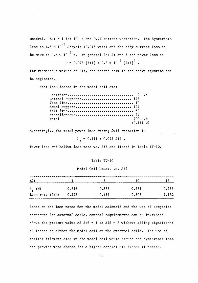
mandrel. ~If = 1 for 10 Hz and 0.1% current variation. The hysteresis

-3 loss is 4.5 x 10 J/cycle (0.045 watt) and the eddy current loss in

holmium is 0.6 x 10-4 W. In general for ~I and f the power loss is

P = 0.045 [~IfJ + 0.5 x 10-4 [~If]2 •

For reasonable values of ~If, the second term in the above equation can

be neglected.

Heat leak losses in the model coil are:

Radiation................................. 9 J/h Lateral supports.................... 145 Vent line ................................. 10 Axial support............................ 127 Fill line................................. 62 Miscellaneous. . . . . . . . . . . . . . . . . . . . . . . . . . . .. 47 Total 400 J /h

(0.111 W)

Accordingly, the total power loss during full operation is

Pt

= 0.111 + 0.045 ~If •

Power loss and helium loss rate vs. ~If are listed in Table IV-10.

Table IV-IO

Model Coil Losses vs. ~If

======================================================================== ~If

P t (W)

Loss rate (i,/h)

1

0.156

0.223

5

0.336

0.484

10

0.561

0.808

15

0.786

1.132

Based on the loss rates for the model solenoid and the use of composite

structure for external coils, control requirements can be increased

above the present value of ~If = 1 to ~If = 3 without adding significant

AC losses to either the model coil or the external coils. The use of

smaller filament size in the model coil would reduce the hysteresis loss

and provide more chance for a higher control ~If factor if needed.

53

IV.5. Drag Coil Requirements

Are drag coils required? The answer is yes, at least one drag coil

is required. Practically it is better to have two drag coils to mini-

mize ampere-meters. The proof is as follows:

Case I: Consider the use of the 4 Z coils to produce the drag

force, lift force and pitch moment. First specify F and F at both J x z

pole tips of the model coil which is 4 constraints. An extra constraint

dB dB = 0 in the XZ plane, ~ = ~

aZ aX to be satisfied is V X B

Thus we have 5 constraints and 4 Z coils which means we need at least

one drag coil.

Case II: Similar arguments can be applied for the use of the 4Z

and 4Y coils to produce drag, lift, and side forces plus pitch and yaw

moments. Now we have 6 forces to specify at model pole tips and three

other constraints from V x B 0, i.e., 9 constraints and 8 coils.

Again one drag coil is needed. For symmetry two drag coils would be

preferred.

54

V. STRUCTUF_~ ft~D THEF1LA~ DESIGN

V.I. Structure Concepts

There are four structural design drivers:

1. Size and location of the magnets.

2. Magnet forces and torques.

3. Choice between individual or one common magnet cryostat.

4. Design and material selection to minimize eddy current losses.

In the 1984 design it was determined that there were significant

structural and thermal advantages to having all of the magnets in a

common cryostat. This arrangement allowed the magnets to be as close as

possible to the wind tunnel and to each other and eliminated the ther­

mally inefficient transfer of forces from cold to warm and back to cold

structure. It was also learned that metallic structure eddy current

losses had the major impact on the size and cost of the cryogenic

system.

The new structural design retains the best features of the 1984

design and incorporates several improvements. Aside from the continuing

use of a common liquid helium cryostat, the principal retained struc­

tural feature is the low heat leak load-bearing "egg-crate" thermal­

vacuum enclosure immediately around the wind tunnel. This gets the

magnet array as close as possible to the tunnel with only a 2 mm thick­

ness stainless steel sheet between the magnets and the model coil. This

thin sheet is essentially transparent to the 10 Hz control field

penetration.

55

1---- 1.25 . - --l II __ "]1

x ~ ~ ~ -0..",,,,',:',,-,,,,,,,,,,,,,,,,,,,,,,,,

B-

I~ , -,

cXJco,e -0.~

x ~m[XJ I [XJ I I : s,,"(_"-E~

\ + \ r---\ I

I ' Iy' ,

<1 ~~r I~-I '

t -t

~ ~ ~ I .. CJ d1 ____ - +.8 G.GOG

B-

Se.CTION A-A

Dimensions are in meters.

Figure V.I. Cryostat Longitudinal Section

56

2..257

~O.5 I~~ f-0.7 ----11

J

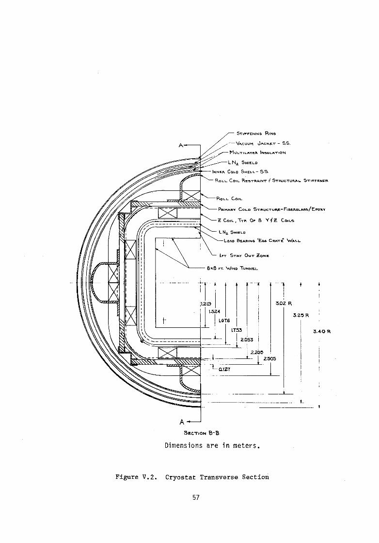
Figure V.2.

STIFFENING R,NG

A ---VACUUM JAC .... ~T - 5.S.

MU1..T'LAYI!tR. h'l~UL"T'ON

LN" SHII!;LD

ROLl .. Call .. RE~T""'NT f S,.."UCTU",,"' .. STI~F~NEFO.

PRIMARY COLD STFO.UCTUI\I!.-FI6E.R6\"A'5~/EpOl<Y

i!: COIL, Typ. a .. 8 y {~ COILo;.

LN2. 5HI~\"D

LOAD BE.ARING "EGG CRATE \NALL

iFT STAY OUT 20NE

8x8 FT. \NINO TUNNE.L

I 1 Tj 1'2~ 1

11.524 I

I \.1m; I

1 I I ; I

3.02 F\

t- I--UT+ I I

'2.200 -

* - LZ.505

-Lo.1Z"T 1

3.Z!5 R

__ ----1--

L

3.4-0 R

------------------

A SECTION B-B

Dimensions are in meters.

Cryostat Transverse Section

57

The principal new structural design feature is the separation of

magnet structure from helium containment. As shown in Figs. V.1 and

V.2, all of the control magnets are attached to a freestanding struc­

tural assembly which is not fastened to the cryostat walls. Further,

except for longitudinal corners and end assemblies, the structure is

epoxy-fiberglass which produces no eddy current heating. Both the inner

and outer cold walls of the cryostat have longitudinal electrical breaks

and the combination end plate/drag coil containment assemblies each have

radial breaks. These features reduce full load structural eddy current

losses from 1560 to 200 w.

Compared to the 1984 design, the overall size and weight of the

MSBS assembly is reduced, the length is increased by 0.2 m because of

the re-positioned drag coils and the diameter is smaller. The vacuum

jacket diameter over the drag coils is now 6.5 m. The weight of the

cryostat assembly and magnet attachments is 125,310 kg, a reduction of

35.2%. Costs are reduced by a somewhat greater percentage despite the

higher base cost of fiberglass-epoxy compared to stainless steel,

because field fabrication and assembly labor are less.

Fewer drawings were prepared for the current work because of its

similarity to the 1984 MMI concept design and the more specific task

focus. Thus, Figs. V.1 and V.2 are the principal representations of the

new design. These sectional views do not include overall longitudinal

dimensions, and support legs are not shown; but other mechanical details

and dimensions are reasonably complete. These two figures are supple­

mented by several detail drawings. Electrical break concept designs for

the end assemblies, cylindrical cold shell and egg crate cold wall are

shown in Figs. V.3, V.4 and V.5, respectively. A view of the stainless

58

steel end plate assembly is given in Fig. V.6 and a section of the roll

coil restraint tunnel is sho~m in Fig. V.7. Discussion of details

illustrated in these figures is included in following sections.

V.2. Materials

Materials for the cryostat are selected for low temperature

compatibility, optimum properties and cost. The material list with

principal applications and properties follows:

304 S.S.--Used for inner and outer walls of the cryostat and for

external stiffening rings. Design stress = 129.6 MN/m2•

304N--Higher strength version of 304 stainless steel used for the end

plate assemblies and corner brackets. Design stress = 137.9

MN/m2•

Nitronic 40 (UNS 521900)--Used for high strength cryogenic bolts and

pins. Room temperature ASME stress = 155.13 MN/m2.

Invar--Invar is useful for washers because of its low shrinkage in

cooling to helium temperature. Although working stress is not

a big factor, the ASME allowable for Invar is 115.8 MN/m2•

G-I0 and G-ll Fiberglass-Epoxy--Main structural slabs and the roll coil

tunnels will be made of epoxy-fiberglass which should have

properties equal to G-I0. Weight-bearing portion of the egg

crate assembly will be made of commercial G-ll because of its

superior vacuum properties. Maximum design stress for these

composites is 137.9 MN/m3 •

59

Dimensions are in millimeters.

INaUI.ATI"IQ CVLINO ....

MS<O'S.5 BocT,UNSS2.1S00

INV" .... W .... S'"' .. "

T ... p~ .. PIN, UNS 52.1300

BOP.ON/Epox.v I~UL."TINQ WR..AP

"'00 ~0.8

Fl. .... ...". .. G~SET (TYR)

G-II IN~UI.AT'NG Sl4&aT

iMATCH 1\ .. " ... T"'''''~D I-Ioc"$ Fop. ALtclNMII.NT

I<!oa It

NOTES

1. A.CTUAL THIc't'ooNE!l5 0,.. 5TPoUC.TUP.e.

MAY VA.RV

2.. LOCATIO ...... I\ND NUMel!.R.~ O~ PINS f BOL.T.5 5U!fIJI!.CT To LOAD CAL.C.VI.. .... TIONS

Figure V. 3. Structural Electrical Break

60

~

I -eR,<dsTAT COLD 'Wp..LL

I --:32MM, NlTRONIC 40 BOLT

V~SPEL~I=~ =lfj€6G#V}'

TNVAR

Figure V.4. Cold Shell Electrical Break

61

i i

EGG I CRATE.

I

COLD 'WALl..

19 MM, N'TRONIC 4-0 BOLT

LINER

INVAR

-1~ ... \ BORON­

VESPEL ~~~I

.EPOXY

5TA\NLE.55 5TE.E.L

F'-ANGES

Figure V.S. Egg Crate Electrical Break

62

El.-E.c. TRICAL

lJa9 .....-;

-/­.. ~

I~~~-'--~- l.-~-------:- __ --~

~ + r-1.005 "\' 195 '

_____ ::1

Dimensions are in meters.

Figure V.6. End Plate Assembly

63

-.-~--.. - -----1------

0.79

T 0.::30

I I r-~0.40-+--'- 1.0 .----

,

I ~O.\27

Dimensions are in meters.

Figure V.7. Roll Coil Restraint and Structural Stiffener

OFHC Copper--This high quality copper will be used for the liquid

nitrogen temperature shields in the egg crate assembly and in

the outer cryostat wall. Mechanical properties are not a

factor in this application.

Boron-Epoxy--This composite has very high compressive strength and is

useful for insulating washers and flange spacers. Allowable

compressive stress is in excess of 344.75 MN/m2 •

Vespel--Vespel is the DuPont trade name for a series of hard

fluorocarbon compounds which maintain physical stability when

cycled from 4.2 to above 400 K. Vespel is proposed as the

sealing material for electrical breaks.

Multilayer Insulation--Multilayer insulation consisting of double

aluminized (400 to 500 Angstrom) Mylar interleaved with either

glass paper or polyolefin scrim is proposed for the outer

portion of the cryostat.

Perlite--Evacuated Perlite powder insulation is effective in cryogenic

use. The egg crate assembly would be filled with Perlite.

V.3. Forces and Torques

Forces and torques on each magnet are given in Table III-3 for

maximum loadings. Structural calculations assume that these maximum

forces occur simultaneously which results in overly conservative design.

This is the most feasible approach at present.

V.4. Structural Design

The current structural design is simplified by the decision to

separate magnet forces from the cryostat. In this way, both the egg

65

crate assembly and outer cylindrical portion of the cryostat are

designed only to retain helium at a maximum of two atmospheres absolute

and not to react other forces except their own dead weight.

The main structural assembly is shown in Figs. V.l and V.2. It

consists of two 304N stainless steel end assemblies (see Fig. V.6) to

which are fastened four large epoxy-fiberglass slabs. Edges of the

slabs are fixed by four stainless steel longitudinal corner brackets.

Span of the slabs is halved by a center epoxy-fiberglass ring and

additional longitudinal stiffening is provided by the roll coil re­

straining tunnels shown in Fig. V.7. The eight identical Y and Z coils

are clamped directly to the structural slabs using specially fabricated

bolts countersunk into the external surface. Roll coils are mounted on

the outside of the slabs using the ,restraining tunnels of Fig. V.7 to

provide clamp forces. Drag coils are wound onto the end assemblies

prior to fabrication of the rest of the structure.

Assembly steps for the MSBS include:

1. Wind drag coils on end assembly plates.

2. Assemble end plates, slabs, center ring and corner brackets

using bolts and epoxy.

3. Install Y and Z coils.

4. Install roll coils and restraining tunnels.

5. Install complete magnet array and structure into the completed

cylindrical outer portion of the cryostat. (Leg stubs may

need to be shortened from those shown in Fig. V.6.)

6. Slide the complete egg crate structure into the magnet/

structure assembly. Egg crates will be supported off the

corner brackets and ID of the drag coils.

66

7. Install warm and cold end bell assemblies. This is the only

assembly process requiring actual fabrication.

8. Install complete wind tunnel test section inside the MSBS unit

without loading the egg crate structure.

V.5. Electrical Isolation

Use of predominantly fiberglass-epoxy structure greatly reduces

eddy current losses. However, it is still necessary to eliminate

significant remaining closed metallic loops. Principal metallic loops

are the end assemblies, outer cold shell of the cryostat and the cold

wall of the egg crate. Detailed electrical break designs developed for

each of these applications are shown in Figs. V.3, V.4 and V.5.

The end plate electrical break concept shown in Fig. V.3 differs

from the other two because it is purely structural and does not require

vacuum sealing. Thus, this design features a simple G-ll insulating

sheet sandwiched between massive flanges. Integrity of the joint is

achieved with a combination of 56 mm Nitronic-40 bolts and tapered pins

which provide alignment and shear transfer. All surfaces are insulated

to prevent electrical leakage and bolts are provided with Invar washers

to assure tightness of the joint on cooldown.

Electrical breaks on the outer cold shell and egg crate wall

combine vacuum sealing and some structural integrity. The first, Fig.

V.4, is more difficult because the 4.83 mm shell to which it is attached

is under internal pressure which creates a maximum separating force of

0.626 MN/m. The egg crate wall is simpler because it is under external

pressure and the joint (Fig. V.5) is being forced together. Aside from

these differing tensile requirements, both breaks are of similar design

67

in that they utilize sharp triangular ridges which bite into a Vespel

sealing strip, have massive flanges to reduce bending, use high modulus

boron-epoxy strips at the outer edge to force loads on the Vespel, and

shim the Nitronic-40 bolts with substantial Invar washers to make

certain that the joints tighten on cooldown. These joints reflect

current technology for vacuum/cryogenic seals but still warrant a

careful preliminary test program.

V.6. Weight Summary

Estimated weights of MSBS system components are given in Table V-I.

The total weight is 210,000 kg ± 15%, which is 43% less than the 1984

MSBS design. The same support system is used here because its heat

leak, 2.4 W, is only 2.5% of the zero load loss.

Table V-I

MSBS System Estimated Weight

======================================================================== Component Weight

Composite structure Stainless steel internal structure Outer shell and rings Inner cold shell End bells Egg crate assembly Liquid nitrogen shield Multilayer insulation

Cryostat sub-total

Helium--30,000 R,

Magnets Bolts, magnet clamp plates, miscellaneous

Total weight

68

22,290 kg 38,080 18,540 4,880 8,440 4,880 2,040

780 99,930

3,780 80,910 25,380

210,000 kg

VI. THERMAL AND CRYOGENIC SYSTEM

VI.l. Cryogenic Concepts

A schematic of the proposed cryogenic system is shown in Fig. VI.l.

Major elements of the system include the magnet cryostat, helium lique­

fier, helium storage dewar, helium recovery compressor, 18 atm. helium

gas storage, and a cooldown loop. Design of the system is based on the

following criteria:

Reasonable cooldown time of seven to eight days.

Adequate liquid storage to fill the magnet cryostat with

reserve to meet daily operating deficits.

Available liquid storage capacity sufficient to empty the

cryostat without loss of helium.

Liquefaction capacity to maintain scheduled operations on a

continuous basis.

Sufficient compressor capacity to handle the maximum planned

rate of gas evolution without helium loss.

Helium gas storage for all of the helium in the system to

permit an indefinite shutdown.

Considerations relating to the design and operation of each part of the

system are discussed in the following sections.

VI.2. Cryostat Heat Leak

Static heat leak of the cryostat is given in Table VI-I. Over half

of the heat leak, 25.4 W, is due to the egg crate assembly which is

relatively thin, 0.152 m, and utilizes Perlite insulation which is much

less efficient than multilayer. However, multilayer insulation is not

69

" C>

HIGH PRESSURE MAKEUP

LNz ~ ..

PURIFIER

LN,. 1'-."

AMBIENT AIR HEAT EXCHANGER

q::GEND

PSV - SAFETY RELIEF VALVE BD - BURST DISC

LIQUEFIER COMPRESSOR

VACUUM JACKET

TC - TEMPERATURE CONTROLLER TE - TEMPERATURE SENSOR L C - LEVEL CONTROLLER LE - LEVEL SENSOR LNz- LIQUID NITROGEN PCV - PRESSURE CONTROL VALVE

354m3

GAs BAG

VACUUM PUMP

PSV

~~.a •. -r--Y--)

COOL DOW BATH

LNz '1---RECOVERY COMPRESSORS

COOLDOWN HEAT EXCHANGER

MSBS CRYOGENIC SCHEMATIC

FIGURE m .•

PSV

18 ATM HELlU~

GAS STORAGE 37, 085 m3

(21C,1 ATM)

APOR COOLED II KA LEAD ASSEMBLY TYP.

OF 22

IND TUNNEL MAGNET CRYOSTAT

feasible for the cellular structure of the egg crate so the major

concern is to make certain that a good fill of Perlite is obtained to

avoid radiation heat shorts. Projected accuracy of the static heat leak

calculations are -10, +30% for the egg crate and ± 15% for the 15.2 W

balance of the system making the plus side range of 9.9 W, about twice

the projected contingency.

Table VI-1

Static Heat Leak and Cryogen Consumption

.========================================================================

Heat Leak--W

Item Helium Nitrogen

Egg Crate Assembly 25.4 430.3

Lead/Vent Stack 6.0 24.0

Outer Cylinder 5.1 90.5

Legs and Braces 2.4 16.8

End Bells 1.7 30.5

Contingency 4.4 57.9

Totals 45.0 W 650.0 W

Helium Consumption--63.5 liters/hour

Nitrogen Consumption--14.5 liters/hour

71

VI.3. Magnet Power Leads

Each magnet has a pair of leads including one pair for the series

roll coils, for a total of twenty-two 11 kA leads. Since there is

excess helium vapor available in all operating conditions, the leads are

designed to reduce no-load losses. Thus the leads are twice as long as

normal and the vapor cooling rate at full load is 0.08 gis, nearly

double the 0.046 g/s/kA optimum rate for standard leads. Without

increased cooling, full-load lead losses would be twice normal instead

of 46% normal. Reductions in lead losses realized with increased vapor

flows are not free because the cold vapor could otherwise return to the

refrigerator to increase its capacity. However, at full load more vapor

is produced than the refrigerator could accept so excess flow through

the leads-is the most efficient way to utilize the available vapor

cooling. Lead losses presented in Table VI-2 reflect use of all avail-

able vapor for the leads at zero and one-fourth load and flows limited

to 0.08 g/s/kA at full load.

VI.4. Operating Losses

Combined loss values for magnets, cryostat and leads are given in

Table VI-3. These losses determine the size of the cryogenic support

system.

Table VI-2

Lead Losses

======================================================================== Magnet Load

Zero 1/4 Full

Heat Input--W

53 59.3

110

72

Helium Loss--t/h

74.8 83.7

155.2

Table VI-3

Magnet and Cryostat Operating Losses

======================================================================== Source of Loss Zero Load 1/4 Load Full Load

W W W

Magnets 0 214.3 522 Structural eddy current 0 50 200 Leads 53 59.3 110 Static heat leak 45 45 45 Conductor joints 0 3.2 51

Totals--W 98 370.9 928

Helium Consumption--t/h 138.2 523.2 1309.1

In Ref. 2 it was shown that the cryogenic system cost only

decreases about 3% if the MSBS is designed to operate on a five-day week

cycle in which the weekend is used to catch up on the liquid helium

supply. Thus continuous operation seven days per week is chosen.

Assumptions used in sizing the cryogenic system include:

1. Cryostat liquid capacity is 30,000 liters

2. 4000 liters of helium are required for final cooldown of the

cryostat from 20 K to 4.2 K

3. Daily operating sequence includes 2 hours at full load, 8

hours at one-fourth load, and 14 hours at zero load.

Size of the refrigerator/liquefier is based on the operating sequence:

Full load--1310 t/h x 2 = 2,620 t

One-quarter load--524 t/h x 8 = 4,192

Zero load--140 t/h x 14 = 1,960

Total daily requirement-- 8,772 t

Liquefier size = 8,772 x 1.026*/24h = 375 t/h

73

The storage dewar is sized by the daily operating deficit and the

storage requirements listed above.

Daily Liquid Deficit

Full load--(1310 - 375/1.026)(2) 1,889 ~

One-quarter load--(524 - 375/1.026)(8) = 1,268

Total daily liquid deficit 3,157 ~

Required dewar size:

Final cooldown 4,000 ~

Fill empty cryostat 30,000

Daily liquid deficit 3,157

Sub-total 37,157

Contingency 7,343

Helium storage dewar size 44,500 ~

It is assumed that all of the helium in the system may be converted

to gas and stored for an indefinite shutdown. Storage capacity is taken

as 10% more than the dewar capacity gas equivalent and 1 atm of the 18

atm storage is considered unavailable. Thus, the volume of gas to be

stored, measured at 1 atm and 294.3 K, is

v = (44,500~)(1.1)(0.7576 m3/~) = 37,085 m3 g

and the 18 atm physical storage capacity is

v = 37,085/(18-1) = 2,181.5 m3 = (77,036.4 ft 3) g

Sizing of the recovery compressor is based on the maximum liquid deficit

which occurs at full load.

*2.6% allowance for storage and transfer losses.

74

VR

(1310 t/h - 375/1.026) 944.5 t/h x 0.7576 m3 /t

= 715.553 m3 /h.

The recovery compressor size is

VR = 715.553/60 = 11.93 m3/min = (421 cfm.)

This defines the major components of the cryogenic system which are

listed in Table VI-4 and illustrated on Figure VI.l.

Table VI-4

Components of MSBS Cryogenic System

========================================================================

Liquef ier (it /h) .......................................... . Storage dewar (J?,) ••••••••••••••••••••••••••••••••••••••••• Recovery compressor (m3 /min) .....•..•......••••....•...•..•..•

(cfm) .............•....................... System helium charge (mS )......... • •••••••••••••••••••••••••

(l atm, 194.3 K) Gas storage at 18 atm (m3 ) ••••••••••••••••••••••••••••••••••••

VI.5. Component Review

375 44,500

11.9 (421)

37,085

2,182

/'

All of the cryogenic system components utilize existing technology

and commercial experience and there should be no difficulty in locating

mUltiple sources of supply.

Liquefier: The 375 t/h liquefier may not be a catalog size for any

manufacturer but it is not large by industry standards and there are

three or four American suppliers. Although not analyzed for this study,

the helium liquefier is expected to utilize two or, possibly, three gas

expanders with final expansion accomplished in a positive displacement

wet expander. Overall efficiency of this size of liquefier should be in

the range of 17.5 to 20% of Carnot.

75

Dewar: The helium dewar will probably be a vertical unit with

multilayer insulation and an intermediate shield cooled with liquid

nitrogen. Loss rate should be in the range of 0.1 to 0.15% per day.

Three or four American companies have the technical background and

facilities to build this dewar.

Gas Handling: The gas handling system includes the recovery

compressor, gas bag and 18 atm storage. The compressor will be a

three-stage oil lubricated machine equipped with oil removal components

and a small cryogenic purifier so that only high purity helium is

stored. The commercially available 354 mS gas bag provides a low

pressure buffer volume for both the liquefier and recovery compressor.

When the liquefier is down, the gas bag collects dewar boil-off for

periodic pumping into storage by the recovery compressor.

Eighteen atm storage consists of 19 commercial ASME coded propane

tanks, each 2.74 m diameter and 20.12 m long. Although space required

for this tank farm is appreciable, storage at 18 atm approximately

matches the liquefier operating pressure which permits interchangeable

use of the recovery and liquefier compressors.

Cboldown System. Only helium is used to cool down the cryostat to

avoid the possibility of contamination. The system is designed (see

Fig. VI-I) so that both the liquefier and recovery compressors work in

parallel for cooldown. Helium flow for cooldown is approximately 33.18

+ 11.93 = 45.11 mS/min and is directed to a special cooldown heat

exchanger and liquid nitrogen bath which provide the major refrigeration

for cooldown. Liquid nitrogen level in the bath is adjusted for a

maximum gas to cryostat temperature difference of 100 K initially to

limit thermal shock. As the cooldown proceeds the temperature

76

difference is reduced until it is less than 5 K at the end. A blower-

type vacuum pump is used to reduce the final bath temperature to 65 K in

order to get maximum cooling from nitrogen.

Cooling below about 70 K is accomplished by using the liquefier as

a cold gas refrigerator. The liquefier is used in this manner until the

cryostat is cooled to about 20 K where its enthalpy is only 0.04% of the

room temperature value. Cooling from 20 K down to 4.2 K and filling the

cryostat is performed in a continuous liquid transfer from the storage

dewar. About 4,000 i of liquid helium is required for the final cool­

down and 30,000 i used to fill the cryostat.

Liquid and Cold Gas Transfer Lines. Vacuum jacketed helium lines

are indicated on Fig. VI-I. The principal VJ line runs from the dewar

to the cryostat with a cold gas extension beyond the dewar to the

liquefier cold box. This co-axial line consists of a 51 OD x 0.89 rom

wall inner liquid line, 5.5 mm radial insulated vacuum space, 63.5 OD x

0.89 rom inner cold gas tube, 101 OD x 1.24 mm outer cold gas tube and a

152.4 OD x 2.77 mm wall (6 IPS, Sch. 5 pipe) warm vacuum jacket. In

normal liquid service this line will function as follows:

1. Liquid flows in the inner line at 0.07 to 0.136 atm above the

cryostat pressure causing the liquid to be 0.1 to 0.15 K

warmer than liquid and gas in the cryostat.

2. Liquid is throttled to cryostat pressure by the flow control

valve which drops the temperature with production of a small

percentage of flash vapor.

3. Slightly colder vapor returns to the liquefier in the annular

gas passage. This cold gas intercepts heat and creates an

essentially zero heat leak environment for the inner liquid

77

line. The purpose of the insulation space between the lines is to

prevent the two passages from forming a heat exchanger whenever the

return gas is warmer as during cooldown.

Controls and Safety Devices. Since design work to date has been on

major functional components, neither the control systems nor safety

devices are worked out in detail. As shown in Fig. VI.1., the cryostat

is equipped with a level indicator and controller to maintain liquid

above the magnets. Because the pressure rating of the egg crate struc­

ture is limited, the helium reservoir will be protected by a sensitive

pilot-operated relief valve and a parallel burst disc. Each of the 22

magnet leads will be equipped with a flow controller and an overall flow

controller will balance lead flows when flows are less than rated 0.88

g/s per lead. Compressors are equipped with bypass circuits and stan­

dard over and under pressure switches for automatic unattended opera­

tion. As the system detail design evolves, care will be taken to

protect all potential isolated cold volumes with thermal relief valves.

VI.6. Cryogenic System Cost Estimate

Estimated cost of the cryogenic system is given in Table VI.5.

Costs are escalated 4% from the 1984 MSBS estimates (Ref. 2).

VI.7. Cooldown Analysis

Cooldown is based on the estimated 33.18 m3 /min flow from the

liquefier compressor plus 11.93 mS/min from the recovery compressor for

a total of 45.11 mS/min. This flow rate limits cooldown of the cryostat

and it is important to keep the gas to cryostat temperature difference

close to 100 K for as long as possible.

78

Table VI-5

Cryogenic System Cost Estimates

========================================================================

375 ~/h helium liquefier

Dewar--44,500 ~

IB atm gas storage--21B2 m3

Recovery compressor--ll.93 m3 /min

LN2 cooldown system

VJ pipe and valves

Balance of plant*

Total

*No buildings or civil work.

$1,556,000

506,000

561,000

169,000

156,000

104,000

156,000

$3,20B,000

Estimated time for each of the three phases of cooling is as

follows:

300--70 K 130 hours

70--20 36

20--4.2 4

Total 170 hours, 7.1 days

VI.B. General Operating Plan

The operating plan for the cryogenic system from a warm start

includes the following steps:

1. Purge and fill the entire system with helium gas.

2. Start flow of liquid nitrogen to the storage dewar shield and

to the cryostat shields.

3. Start the liquefier and fill the storage dewar. With a

24-hour allowance for cooldown, it will take about six days to

fill the dewar.

79

4. Cooldown and fill the magnet cryostat. Allow a week for this

step.

5. Operate the cryostat as scheduled:

a. ~~enever gas flow exceeds liquefier capacity the recovery

compressor will cycle on to pump gas back to 18 atm

storage.

b. Liquefier is sized to run continuously when there is

liquid in the cryostat and the test regime is followed.

For five-day week operation the liquefier would shut down

or idle over the weekend.

6. At the end of a wind tunnel operating cycle or at any time the

system is to be down more than two weeks, liquid should be

transferred back to the dewar and the cryostat allowed to warm

up to 78 K by continuing to supply liquid nitrogen to the

shields. Restart from this point can be accomplished in about

three days.

7. Since the storage dewar will only lose 1,400 to 2,000 liters

per month, it should be left cold except for very long shut­

downs of three months or more. When the dewar is idling, gas

is collected in the gas bag and is pumped back to 18 atm

storage about once each week to ten days. Pumping the gas

back to storage will take about one-half hour.

8. For long-term shutdown, liquid may be vaporized in the ambient

heat exchanger at a rate consistent with the recovery compres­

sor capacity and pumped to high pressure storage.

80

VI.9. Cryogenic Impact of 1.8 K Operation

Operation at 1.8 K impacts both the cryostat and refrigerator/

liquefier. The cryostat must be modified to provide a normal helium

reservoir for the leads and a thermally insulated passage between 4.2

and 1.8 K for leads. A heat exchanger for 1.8 K, 12 torr fluid to

1.8 K, 1 atmosphere helium must be provided and piping modifications

must be made to limit heat leak into 1.8 K helium. The refrigerator is

modified to provide normal helium for lead cooling and intercepts and

refrigeration to the 1.8 K, 12 torr heat exchanger. In all cases,

enthalpy rise from from 1.8 to 2.0 K for 30,000 liters, ~H = 3.469 x

106 J, is utilized to extend full power operating time.

If the normal operating sequence is used (2 hours at full power, 8

hours at 1/4 load and 14 hours at idle), the size of the equivalent

liquefier is about 845 t/h and its cost is $2,748,000, an increase of

$1,192,000. Estimated total cost increase for this normal operation

option is:

Liquefier addition

Cryostat additions:

Lead dewar & transition

Heat exchanger

Specializing & valves

Total addition

$1,192,000

75,000

150,000

100,000

+ $1,517,000

If 1.8 K operation is a zero cost option, increases in the cryostat

and liquefier must match the $750,000 conductor and magnet saving. This

means that the liquefier increase is limited to $750,000 - $325,000 =

81

$425,000. This buys the equivalent of a 530 Y./h liquefier and provides

the following performance options:

Full load

1/4 load

1.88 hours, or

7.83 hours

Either of these options, or a mix (for instance 1 hour at full load +

3.65 hours at 1/4 load) must be followed by a recovery time of 15.2

hours. Thus, several hours of daily operation at 1.8 K could be sus­

tained with this cryogenic system.

82

VII. COST ESTIMATE

The MSBS cost estimate is $21,398,000 for a system equivalent to

Case l--Alternate G of NASA CR165917 (Ref. 1). It includes control

based on a power amplitude of 0.1% of I in all coils simultaneously max .

at a frequency of 10 Hz. The estimates mostly stem from analyses made

by MMI. However, several topics have not been addressed by MMI, notably

position sensors and the control system, and estimates for these items

have been carried forward from NASA CR 165917 and are marked with an

asterisk (*) in Table VII-I.

The estimated cost of $21,398,000 for the MSBS is a reduction of

$8,541,000 or 28.5% from NASA CR 3802 prepared by MMI in 1984. This

significant cost reduction is attributed to the following factors:

* Increased pole strength of the model core magnet by use of a

holmium mandrel.

* Use of Nd15Fe77B8 permanent magnet material in the model

wings.

* Overall reduction in control magnet sizes due to the above

factors and a more efficient configuration of the roll coils.

* Continued better understanding of the MSBS system.

* More realistic power supply utilization.

* Structural design to minimize eddy current heating.

Costs presented in Table VII-l are not contingent on additional

analytical or experimental efforts but assume that such work would be

accomplished as required. These estimates would be impacted by a future

program addressed to some of the key features of the MSBS by more

accurately quantifying the design parameters. This work would not

83

necessarily further reduce the MSBS cost, but it would improve the

accuracy of the estimate and validate technical feasibility.

Estimates include 4% escalation of comparable items from 1984

except that structure was based on the same $10 per fabricated pound

used previously. Machines and Tooling, 1.3.2, was reduced from

$1,458,000 to $1,000,000 because the X, Y and Z coils are much smaller

than previously and can be wound on commercially available equipment.

This leaves the major portion of the Machines and Tooling budget for

design and fabrication of the Roll coil winding fixture.

84

Table VII-l

MSBS Cost Estimate (Costs in Thousands $)

========================================================================

1.0

1.1 1.1.1 1.1. 2 1.1.3 1.1.4 1.1.5 1.1.6 1.1. 7 1.1.8 1.1. 9 1.1.10

1.2 1. 2.1 1.2.2 1. 2. 3 1.2.4 1. 2.5 1.2.6 1. 2. 7 1. 2.8 1. 2. 9 1. 2 .10

1.3 1. 3.1

1. 3. 2 1. 3. 3 1. 3. 4 1. 3. 5 1. 3. 6 1. 3. 7 1. 3.8 1. 3. 9 1.3.10 1. 3.11 1.3.12 1.3.13 1. 3 .14 1. 3.15 1.3.16 1.3.17 1. 3.18

Complete MSBS System

Preliminary Design Phase System Engineering $ Magnet Preliminary Design Cryogenics Preliminary Design Power Supply and Protection Preliminary Design Position Sensors Preliminary Design Control System Preliminary Design Support Structure Preliminary Design Manufacturing Engineering Quality Control Plan Preliminary Design Phase Program Management

Final Design Phase System Engineering Magnet Final Design Cryogenics Final Design Power Supply and Protection Final Design Position Sensors Final Design Control System Final Design Support Structure Final Design Manufacturing Engineering Quality Control and Testing Final Design Phase Program Management

Manufacturing, Installation and Checkout Phase Engineering Support for Manufacturing,

Installation and Checkout Special Machines and Tooling Manufacturing Z Gradient Coils Manufacturing Y Gradient Coils Manufacturing Roll Coils Manufacturing Drag Coils Model Core Magnet and Cryostat Cryogenic System Power Supplies and Protection Systems Position Sensors Control System Support Structure and Cryostat Quality Control and Testing Not Used Packing and Shipping Assembly and Installation Checkout and Acceptance Testing Manufacturing, Installation, Checkout

Phase Program Management

100 150 60 30

130* 90*

140 20 40

115

150 300 275 100 420* 350* 445 175 175 375

680 1,000

381 381

1,039 802 150

3,198 2,028 1,068* 1,046* 2,198

175

250 1,000 1,012*

1,350

$21,398

875

2,765

17,758

*These values taken directly from NASA CR 165917 for Case 1, Alternate G

85

VIII. APPENvICES

Appendix A. Magnetic Pole Strength of a Superconducting Solenoid with Holmium Mandrel.

Appendix B. Roll Torque Analysis.

Appendix C. Force and Torque Requirements.

Appendix D. Cross Coupling Analysis.

Appendix E. Optimization of Drag and Roll Coils.

Appendix F. Tunnel Wall Constraints.

87

APPENDIX A

MAGNETIC POLE STRENGTH OF A SUPERCONDUCTING

SOLENOID WITH HOLMIUM MANDREL

Assume the following superconducting coil nomenclature:

J = gross current density in winding

b winding outer radius

a winding inner radius and holmium outer radius

c = holmium inner radius

~ = holmium magnetization a function of magnetic field

For a long solenoid (L»2b), the maximum field at the winding is at the

midplane,

B = ~ J (b - a) • m 0

A.I

The magnetic pole strength of the winding, ~, and of the holmium, Qh'

are

and

3 3 o = ~J (b - a )/3, 1ll

2 2 Qh = ~~ (a - c )/~o •

The total magnetic pole strength is

Q 3 B 3 B 2 2

~J {b - (b-~) } /3 + ~M {(b-~) - c }/~ ~ J h ~ J 0 o 0

89

A.2

A.3

A.4

APPENDIX B

ROLL TORQUE ANALYSIS

The wing configuration used in this analysis is that of the F16

fighter model. The arrangement of the wing plan form is shown in Figs.

B.1 and B.2. Using the non-dimensionalized airfoil coordinates provided

by NASA, the cross-sectional area A at any chord of length C is

A = 0.02625 C2 2 cm B.1

At the tip C = 9.8 cm and A = 2.52 cm2 while at the fuselage C 43.18

cm and A = 48.9 2 cm • Actually, the wing begins at y = 6 which is the

outer radius of the model core and extends to y = 41 cm at the tip. The

cross-sectional area at any distance y is

2 A(y) = 48.4 - 1.8453 y - 0.0173952 Y 2 cm B.2

Taking M as the average magnetization in the y direction, it is easy to

show that the net torque is

2 b T = -- {bMa(b)B (b)-aMA(a)B + MJ B R(y)ydA } r]1o z z a z y

B.3

where a = 0.06 m, b = 0.41 m, and BzR(y) is

BzR(y) B (b) Y z b·

91

'>:j .,.. OQ c:: Ii ID

td · ...... · lD N '>:j

......

'" ~ .,.. ::t

OQ ·

o OJ

N

0 . ~ 01 N 3

€ ~01=0.06m 1------ b = 0.41 m-----f

1.0 W

z Ie

0.3

0.2 NACA 64 A204 AIRfOIL SECTION

0.1

o xk

5.5. SUPPORT -0.1

-0.21 I I t I I , , , I _1-_ o 0.1 0.2 0.3 0.4 0.5 0.6 0.7 0.8 0.9 1.0

x/c

Figure B.2. Wing cross-sectional area at any chord length C showing stainless steel support, skin, and permanent magnet material.

Band M are in tesla while distances are in meters and T is in Nm. z r

From the above equations, the magnetic field BzR(b) at the tip of

the wing is

B (b) ZR

~ 471"10-4 Tr(O) M

where T (0) is the torque at zero roll angle~. To produce the required r

torque of 141 Nm at ±20°,

2 0 • 2 0 T (0) = 141/(cos 20 - s~n 20 ) = 184 Nm. r

B.6

Equations B.5 and B.6 are used to calculate the roll coil field at wing

tips.

94

l>.PPEND IX C

FORCES AND TORQUE REQUIREMENTS

The requirements for static forces and moments are listed in Table

C-1. If the model is replaced by a magnet of a length L and a pole

strength Q, then the force in the ith direction for + B. at the north 1

pole and B. at the south pole (typical of MSBS fields) is 1

F. = 2Q B. 1 1

where: F. = force in the ith direction (N ) 1

Q = model magnet pole strength (Am)

C .1

B. magnetic field in the ith direction at the core tips (T) 1

i x, y, or z.

The magnetic field at the poles of the core, B., is the field due to all 1

coils in the ith direction at any position of pitch and yaw.

The pitch and yaw torques are

T = Q L oB cos a , p z

C.2

and T = Q L oB cos B , y y C.3

where oB and oB are the difference in Band B at the two end model

tips.

z y z y

oB appears in Eq. C.2 because the F forces at each end of the zz

pole tip are in the same direction and result in the torque only if one

Fz1 = Q Bz1 is larger than Fz2 = QBz2 ' or oB IBz1 - BZ21> O. The

pitch and yaw angles are a and B.

95

Table C-1

MSBS Requirements, 8' x 8' Test Section

========================================================================

A. Static Force Requirements

Lift Side Drag

B. Static Moment Capability

Pitch Yaw Roll

C. Angular Displacement Range

Angle of Attack (a) Angle of Sideslip (8) Angle of Roll (~)

D. Core Dimensions

Length Diameter

E. Wing Dimensions

F. Dynamic Force Requirements, ± 0.1% at 10 Hz

Lift Side Drag

The roll torque at any roll angle ~ is

T ~ 2 q b B R {cos2 ~ - sin2 ~} , r z

9790 N 1380 N 4180 N

420 Nm 140 Nm 140 Nm

± 30° ± 10° ± 20°

75 cm 12.7 cm

(see Figs. B.1 and B.2 in Appendix B)

± 9.79 N ± 1. 38 N ± 4.18 N

C.4

where q is an equivalent magnetic pole strength of the permanent magnets

in the wing tips and 2b is the equivalent span. Details of roll torque

calculations are provided in Appendix B. BzR is the z component of the

magnetic field at the tip of the wing for ~ = O.

96

APPENDIX D

CROSS COUPLING ANALYSIS

An ideal situation for the MSBS would be for all coils to function

independently. Unfortunately this is not possible when the model plane

pitches, yaws or rolls. Then there are some minor cross couplings and

some major cross couplings. When the model is at zero angle of pitch,

yaw and roll, there are no cross couplings between any group of coils

with any other group of coils. When the model pitches, yaws or rolls,

cross coupling occurs. For larger angles the cross coupling is larger.

Hence the largest angle of pitch, ± 30°, will cause the highest mode of

cross coupling. The arrangement of magnetic material in the model wings

(positive poles are at wing tips while negative poles at fuselage) will

result in no roll moment or force from the X, Y or Z coils. Conse-

quently, the R coils suffer no cross coupling from the X, Y or Z coils

while the latter suffer from the high R coil field. Therefore, we

emphasize the X, Y and Z coils which are subject to cross coupling from

the R coil.

Drag Coils (X Coils)

The drag coils have no cross coupling with the R coils because the

main current in the R coils is in the x direction which produces no B x

component. When the model pitches, there is cross coupling between the

B component from the Z coils and the X coil B field. This component x x

may be calculated from V x B O. Similarly, as the model yaws, there

is cross coupling between the B component of the Y coils and the X coil x

B field. Unfortunately, these two cross coupling components act x

97

against the required B component. At angles a and S in pitch and yaw .x

the B component is related to the x, yand z field component of the X, x

Y and Z coils, respectively, as

B x B cos a cos l3 - B sin S - B sin a , xo yo zo

where: B is the x component due to the X coils at a = S = 0 xo .

B is the y component due to the Y coils at a = S 0 yo .

B is the z component due to the Z coils at a = S 0 zo

Z Gradient Coils

D.l

When the model pitches or yaws, the total z component at the model

tip will be the sum of the z component due to the Z coils, a cross

coupling z component from the X coil, and a cross coupling z component

from the R coils.

The cross coupling component from the X coil during pitch may be

found from V·B = 0 and is + B /2 sin a • . xo

When the model core yaws, the model coil tips experience a B z

component field produced by the R coils. This B field from the R coils z

produces a net F force (no pitch toraue) on the model core. This force z •

is equal to slightly less than one-third of the maximum F required on z

the model. Correction is made by increasing the ampere-meters of the Z

coils to balance the undesired z force from the R coils. The undesired

B component during yaw is related to the z component from the R coils z

at the wing tips, BzR ' as

B = B R (L/2b) sin 8 = A sin S • z z

where L is the model core length and 2b is the wing span.

98

D.2

The total maximum possible B field at angles a and S in pitch and z

yaw is

B z

B cos a + B 1/2 sin a - A sin S • zo xo

In the above equation, cross coupling from the X coils will always

strengthen the reQuired B component during pitch (positive cross - z

D.3

couplings) while the z component from the R coils during yaw may add to

or subtract from the net B field depending on the angles of roll and z

yaw.

Y Gradient Coils

There is a positive coupling y component from the X coils equal to

(+ 1/2 sin S) Bxo D.4

~~en the model core pitches, the end tips experience a B component y

from the R coil which translates into a net undesired F side force. y

The undesired B field component is y

B = B R L/2b sin a = A sin a • y z

This y component from the R coils causes a serious cross coupling

D.S

problem; unfortunately th~re is no apparent solution except for making

the Y gradient coils large enough to take care of this undesired field

component.

99

The total required By field at angles of a and S in pitch and yaw

is

B = B cos a cos S + 1/2 B sin S - A sin a • y yo xo D.6

100

APPENDIX E OPTIMIZATION OF DRAG AND ROLL COILS

E.l Procedure

The procedure to optimize the ampere meters "IS" of the drag

and roll coils is as follows:

1) Express the required x-field at the poles of the model

magnet due to the drag coils in terms of drag coil design

parameters and locations.

2) Express the required z-field from the roll coil at the wing

tip in terms of roll coil design parameters and locations.

3) Write an expression for the total ampere-meters in the

drag and roll coils as a function of the dependent

variables.

4) Write the constraints on the optimization.

5) Optimize equation (3) subject to the constraints of (4).

E.2 Magnetic Field Due to Drag Coils at Model's Pole

where

The field at point Q (Fig. E.l) is

B = H x 0

F(a, ~1 + S) - F(a, ~1- S)

[ 2F(a, S)

a

~1

F(a, ~2 + S) - F(a, ~2 - S)

2F(a,B) ~

1 + .!. t

p + q/2 - z t

q S = 2t

~2 = P + q/2 + z

101

(E.l)

...... a N

-n ..... (Q

c: ""S (1)

IT1 .

-n ..... (1) --' Q.

0 c: (1)

M-0

n c: ""S ""S (1) ::s M-

Vl ::l"' (1) (1) M-

CD >C

~ » ~I

.......-IN ........ Q.

1+ t

CT

0<

0

1 0 x CD

\' \\ \'

'..-~-..I \' \' \\

1\\ \ \ \ , ' \ , \ \,

ro N

F(a, 8) B tn a + la2

+ 82

and 1 + 11 + 82

Ho llo JtF(a,8) •

Substituting in (E.l)

II 'Jt Bx= -T [F(a,8+~l) - F(a'~l--B) - F(a'~2+8) + F(a'~2-8)]

(E.2)

E.3 Magnetic Field Due to the Roll Coil at Wing Tip

To calculate the magnetic field due to the roll coil, let us

first find the field due to a current sheet of thickness ~, height

2b, and length A.

For a current element J~dz (Fig. E.2) in the y-direction, the

field dB at point 0 is z

doB z

II J~dz o

41T cos</> cose dy ,

2 r

where c

y = c tan</> r =--cos</>

dy c

2 cos </>

Substituting

d</>

II J~ cose dz 2 doB o c cos¢ cos </> d</>

Z 41T 2</> 2 cos c and

103

and

~ 1

x I @

ro o

~\ ~~

~ ,flJ ,\0,\<$

B® + -1- ~+QI I

...--2y--...

l 2g

t •

I I-k 'I' { 1

I

rn@ Figure E.2. Quadrupole Field of the Roll Coil at

the Model Wing Tip

:.J + Q

t-2z-

I I r P ... ql-

t f f t t

Figure E.3. Field on the Axis of the X-Drag Coil

104

CD

Jl Jfl case dz +B o B = a 4 f cos<j> d<j>

z 'IT C -S

= Jl a Jfl sinS 2'IT cease dz •

Integrating over length 2b

a B

z

Jl Jfl sinS o

2'IT C f c case 2 de ,

cos e -a

a f ~--a case - tn tan (2!.. e) 4+"2 la = tn tan ('IT /4+a/2)

-a tan ('IT /4-a/2) 2 tn l+tan(a/2)

I-tan(a/2)

or fa ~ = tn (l+Sine) cose cose la (l+Sina) •

= tn I-sina -a -a

~ Jfl l+sina) B = _o~ sinS tn( l-sina z 211"

(E-3)

-1 1 height ) where a = tan ("2 ~~~~~, A~~~~~~a and

-1 1 length ) • 8 tan (2 normal distance

In general if the current element is enclosed by aI' a 2 (Fig.

E.3)

105

11 JI::. B = __ 0 __ (sin8 - sinS )

z 41T 2 1

a J 2~

a cose' 1

or

110JI::.. . (l+sina 2) cosa 1

Bz =~ (s ln8 2 - Sl uS 1) R.n [(1.L~':_~ \ ~~M"]

The field in the x-direction,

and

dB x

B x

11 0 JI::. (sin8 2 - sine 1 ) . = 4'J1' Slne dz ,

11 0JI::.(sine 2-sin8 1) t2 sine c

2 de ,

a cos e 1

11 JI::. B = 0 x 41T (sin8 2-8 1) 1 ~]

(E.4)

(E. 5)

Now, for the arrangement of roll coil as shown in Fig. (E.4)

the z-field due to each coil (1) and (2) at pole tip Q1

11 Jk I+Sina] B = __ 0_ sin 8 R,n [I-sina • z 21T

Substituting for

106

I J = kg

where I current flowing in one conductor

Bzl ~ I l+sina 1

= -20

sinS 1£ n [1 . 1 ng _~'~N ] Bz2 ~ I l+sina

2 = - -2

0 sinS 2 £n [1 . ] 1Tg -s1na 2

For coil (1) at Ql

-1 e j ) 13 1 tan ?(O_u.1,!?' -Ie' g ) a 1 = tan 0 _.,.1. !?

For coil (2) at Ql

-1[ j ] 13 2 tan ? (0 .. ,.1, !?, -Ie g ) a 2 tan o .. ,.1,!?

For coil (3) at Ql

lloI 1 B = - sinS [--z3 21Tg 3 cosa4

1 ]

For coil (4) at Ql

1l0I 1 1 B = - sinS [ - ~

z4 21T g 4 cosa 6 cosa 5

-1 [ j 1 13 3 = 13 4 = tan ?In., .. .1.!,>,]

107

a 3 = a 5

a4

= a6

-1 y-g] = tan [t+k/2

-1 y+g] = tan [t+k/2

Total z-field at Q1' B = B 1 - B 2 + 2B 3 z z z z

\l Jk 1+si00 1 1+si00 2 Bz= ~'IT [sinS 1tn(1_sina.) - sinS2tn(1_~.f~~)

1 ~ 1 )] + 2sinS 3( cosa 4 cosa 3

E.4 Total Ampere Meters in the Drag and Roll Coils

The ampere-meters of the two drag coils is

IS = 2'IT(2t + f) Jqf , x

where J is the current density

t, f, q are as shown in Fig. E.3.

The ampere meters in the roll coil are

IS = 4( 2j + 2'ITr 1 + 'ITr 2) Jkg , r c c

where j, k, g are as shown in Fig. E.2.

108

(E.6)

(E.7)

For r . 0.5 m Cl

rc2 1.2 m and

J current density, we get

IS = (8j + 27.646) Jkg r

and IS t 1 21T (2t + f) Jqf + (8j + 27.646) Jkg • to a

E.5 Optimization Constraints

The constraints on the optimization are as follows:

(1) For the roll coil B = constant = F /Q1 z z

(2) For the drag coils B = constant = F /Q2 x x

(3) The distance y constant 0.41 m

(4) The distance z = constant 0.35 m

(5) The distance R. constant = 2.204 m

(6) The current density J = constant

(7) The distance t = constant = 2.257 m

E.6 Optimization

(E.8)

To carry out the optimization, let us recall the equations for

the magnetic field due to the drag coils,

where

l.l Jt Bx = -1-- F 2 (a, B, S l' S 2) ,

F 2 (a, S, S l' S 2 ) F 3 (a, S 1 + B) - F 3 (a, S 1 - B)

- F 3 (a, S 2 + B) + F 3 (a, S 2 - B)

109

(E.9)

F 3 (a, f3) f3 In

Rearranging (E.9)

a + .,Ia. 2 + f32

1 +.,11 + f32

2B t F2(a, f3, ~1' ~2) = ~ = constant.

~o (E.10)

In the same manner, recall the equation for the magnetic field

due to the roll coil

]J Jk

B z = ~'IT [ F 1 ( a l' a 2' a 3' f3 1 , f3 2' f3 3) ] (E.11 )

where F1 is as shown in equation (E.6).

Rearranging Equation (E.11)

2'IT B kF1(a 1, a 2 , a 3 , f3 1 , f3 2, f3 3) = / = constant

]Jo (E.12)

A computer program is used to minimize equation (E.8) subject to the

conditions of equations (E.11) and (E.12).

110

APPE1lDIX F

TUNNEL WALL CONSTRAINTS

The 10 Hz requirement for dynamic field control requires that a 10

Hz field variation must be transmitted through intervening walls. In

NASA CR-i65917[1] this problem was approached by estimating the time

constants for field diffusion through the intervening wall. The

intervening wall was modeled as an infinite cylinder between the magne,t

system and the airplane model. Table E-1 reproduces the field diffusion

chart with an additional entry for the presently planned MMI low

temperature 2 rom thick stainless steel wall.

If the test section has a time constant comparable to T 0.1 sec

then severe field wave form distortion results. Note that the MMI wall

thickness of 2 mm has a time constant about 1/3000 of the field driving

time constant and would produce no distortion.

A similar conclusion can be drawn from skin depth 0 which measures

depth of penetration of an incident wave. The skin depth is the

distance within a conductor at a point at which the amplitude of the

field vector is equal to l/e = 0.3679 of its value at the surface.

1/2 o = (2p /llW)

-1/2 = 36 f cm for S.S. at low temperature

= 11.4 cm at 10 Hz.

A wall 2 mm thick is almost transparent at 10 Hz and quite transparent

for control frequencies up to 200 Hz.

111

Table F-1

Time Constants for Field Diffusion Through Dewar Walls

8' x 8' Test Section

~=======================================================================

MMI Design Design of Ref. 1

Wall Thickness 2mm 25.4 mm 50.8 mm 76.2 mm

Stainless Steel* 0.0000315 sec 0.005 sec 0.02 sec 0.045 sec

Characteristic T ~ l/f = 0.1 sec time at 10 Hz

-8 *p = 50 x 10 am at low temperature.

112

1. Report No. I 2. Government Accession No. 3. Recipient's Catalog No.

NASA CR-3937 4. Title and Subtitle 5. Report Date

October 1985 MAGNETIC SUSPENSION AND BALANCE SYSTEM ADVANCED STUDY 6. Performing Organization Code

7. Author{s) 8. Performing Organization Report No.

R. W. Boom, Y. M. Eyssa, G. E. McIntosh, and M. K. Abdelsalam 10. Work Unit No.

9. Performing Organization Name and Address

Madison Magnetics, Inc. 11. Contract or Grant No. 216 Walnut Street Madison, Wisconsin 53705 NAS1-17931

13. Type of Report and Period Covered 12. Sponsoring Agency Name and Address Contractor Report

National Aeronautics and Space Administration 12L84iO _6/85

Washington, D.C. 20546 14. Sponsoring Agency Code

505-31-53-10 15. Supplementary Notes

Langley Technical Monitor: Richmond P. Boyden Final Report

16, Abstract

An improved compact design for a superconducting magnetic suspension and balance system for an 8 ft. x 8 ft. transonic wind tunnel is developed. The original design of an MSBS in NASA CR-3802 utilized 14 external super-conductive coils and a superconductive solenoid in the airplane test model suspended in a wind tunnel. The improvements are in the following areas: test model solenoid options, dynamic force limits on the model, magnet cooling options, structure and cryogenic designs, power supply specifica-tions, and cost and performance evaluations. The improvements ate: MSBS cost reduction of 28%, weight reduction of 43%, magnet system ampere-meter reduction of 38%, helium liquefier capacity reduction by 33%, magnet system stored energy reduction by 55%, AC loss to liquid helium reduced by 76%, system power supply reduced by 68%, test coil pole strength increased by 19%, wing magnetization increased by 40%, and control frequency limit increased by 200% from 10 Hz to 30 Hz. The improvements are due to: magnetic holmium coil forms in the test model, better rare earth permanent magnets in the wings, fiberglass-epoxy structure replacing stainless steel, better coil configuration, and new saddle roll coil design.

I

17. Key Words (Suggested by Author(s)) 18. Distribution Statement Magnetic suspension Magnetic balance Superconducting magnets Unclassified - Unlimited Wind tunnel balance

Subject Category 09

19. Security Oassif. (of this report) 20. Security Classif. {of this pagel 21. No. of Pages 22. Price

Unclassified Unclassified 126 A07

For sale by the National Technical Information Service, Springfield, Virginia 22161 NASA-Langley, 1985