Magnetic Maps of Indoor Environments for Precise Localization of

Legged and Non-legged Locomotion

Martin Frassl1, Michael Angermann1, Michael Lichtenstern1, Patrick Robertson1,

Brian J. Julian2,3, Marek Doniec2

Abstract— The magnetic field in indoor environments is richin features and exceptionally easy to sense. In conjunctionwith a suitable form of odometry, such as signals producedfrom inertial sensors or wheel encoders, a map of this fieldcan be used to precisely localize a human or robot in anindoor environment. We show how the use of this field yieldssignificant improvements in terms of localization accuracy forboth legged and non-legged locomotion. We suggest variouslikelihood functions for sequential Monte Carlo localizationand evaluate their performance based on magnetic maps ofdifferent resolutions. Specifically, we investigate the influencethat measurement representation (e.g., intensity-based, vector-based) and map resolution have on localization accuracy,robustness, and complexity. Compared to other localizationapproaches (e.g., camera-based, LIDAR-based), there exist farfever privacy concerns when sensing the indoor environment’smagnetic field. Furthermore, the required sensors are lesscostly, compact, and have a lower raw data rate and powerconsumption. The combination of technical and privacy-relatedadvantages makes the use of the magnetic field a very viablesolution to indoor navigation for both humans and robots.

I. INTRODUCTION

A. Motivation

Precise localization of humans and robots in indoor envi-

ronments is an essential component for numerous applica-

tions. Existing technical solutions to indoor localization ei-

ther rely on (i) infrastructure, such as radio beacons, passive

or active transponders, guiding wire, and/or optical markings;

or (ii) onboard sensors, such as LIDAR (Light Detection

and Ranging), monocular cameras, and/or stereo imaging.

Recent insights into the structure of the indoor magnetic field

have triggered strong interest in the potential use of this field

for localization purposes. Firstly, the indoor magnetic field

typically shows strong modulation with spectral components

over a wide spatial bandwidth (e.g., [1 m−1, . . . , 0.01 m−1],or even wider), suggesting the capability to acquire robust

This work is supported by DLR under Project Dependable Navigation.This work is sponsored by the Department of the Air Force under Air

Force contract number FA8721-05-C-0002. The opinions, interpretations,recommendations, and conclusions are those of the authors and are notnecessarily endorsed by the United States Government.

1M. Frassl, M. Angermann, M. Lichtenstern and P. Robertsonare with the Institute of Communications and Navigation of theGerman Aerospace Center (DLR), 82234 Wessling, Germany, mar-tin.frassl@dlr.de, michael.angermann@dlr.de, m.lichtenstern@dlr.de andpatrick.robertson@dlr.de

2Marek Doniec and Brian J. Julian are with the Computer Scienceand Artificial Intelligence Laboratory, MIT, Cambridge, MA 02139, USA,doniec@mit.edu and bjulian@mit.edu

3Brian J. Julian is also with MIT Lincoln Laboratory, 244 Wood Street,Lexington, MA 02420, USA

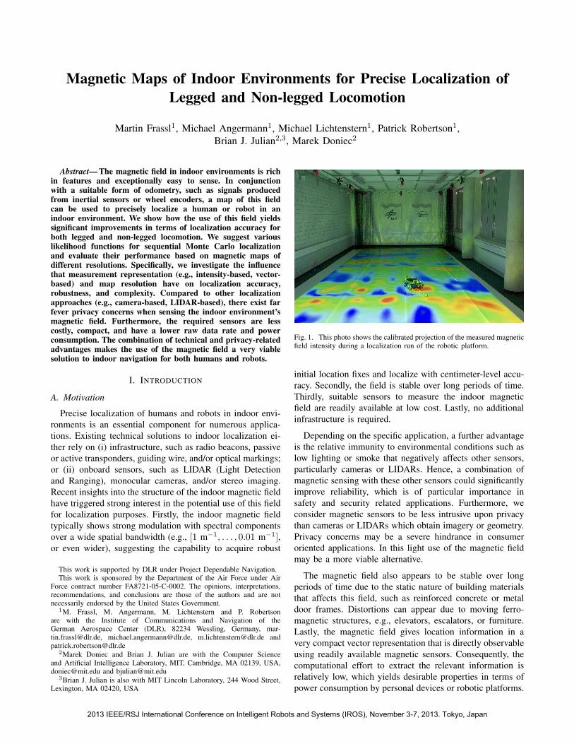
Fig. 1. This photo shows the calibrated projection of the measured magneticfield intensity during a localization run of the robotic platform.

initial location fixes and localize with centimeter-level accu-

racy. Secondly, the field is stable over long periods of time.

Thirdly, suitable sensors to measure the indoor magnetic

field are readily available at low cost. Lastly, no additional

infrastructure is required.

Depending on the specific application, a further advantage

is the relative immunity to environmental conditions such as

low lighting or smoke that negatively affects other sensors,

particularly cameras or LIDARs. Hence, a combination of

magnetic sensing with these other sensors could significantly

improve reliability, which is of particular importance in

safety and security related applications. Furthermore, we

consider magnetic sensors to be less intrusive upon privacy

than cameras or LIDARs which obtain imagery or geometry.

Privacy concerns may be a severe hindrance in consumer

oriented applications. In this light use of the magnetic field

may be a more viable alternative.

The magnetic field also appears to be stable over long

periods of time due to the static nature of building materials

that affects this field, such as reinforced concrete or metal

door frames. Distortions can appear due to moving ferro-

magnetic structures, e.g., elevators, escalators, or furniture.

Lastly, the magnetic field gives location information in a

very compact vector representation that is directly observable

using readily available magnetic sensors. Consequently, the

computational effort to extract the relevant information is

relatively low, which yields desirable properties in terms of

power consumption by personal devices or robotic platforms.

2013 IEEE/RSJ International Conference on Intelligent Robots and Systems (IROS), November 3-7, 2013. Tokyo, Japan

B. Magnetic Field Characteristics

The characteristics of the undisturbed earth magnetic field

depend on both the location and time of the observation.

The magnitude of the temporal change is relatively small

with daily fluctuations between 10 nT to 30 nT, which is

less than 0.1% of the average magnitude of 48.19 µT seen

in our geographic region [1]. The spatial change, however,

has a significant influence on the direction and magnitude

of the magnetic field. The magnetic field vector roughly

points in the direction of geographic north, but is more

accurately represented by its declination and inclination. The

declination describes the horizontal deviation of the direction

from the geographic north, while the inclination describes the

vertical component of the field. Approximate values of 145′

declination and 64◦ inclination are reported at the location

of our lab facilities (48.08◦ N, 11.28◦ E) [1]. Inclination and

magnitude of the magnetic field vector are lowest around the

equator and roughly increase with increasing latitude.

The ubiquitous magnetic field is further disturbed by

manmade structures. In particularly, the magnetic field is

influenced in proximity of ferromagnetic materials used in

the construction of buildings - a comprehensive analysis of

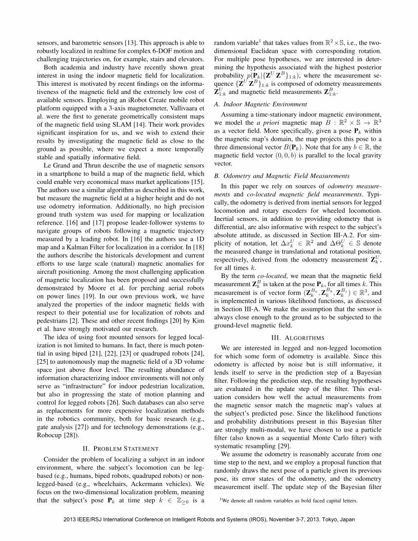
this property can be found in [2]. For example, Fig. 2 shows

the intensity of the magnetic field at ground level within

our motion capture laboratory. This intensity varies varies

between 0 µT and 120 µT, which is a range that is factors

of 2.5 and 104 compared to the intensities of the undisturbed

magnetic field and its daily fluctuation, respectively.

−4 −2 0 2 4y [m]

−2.0

−1.5

−1.0

−0.5

0.0

0.5

1.0

1.5

x[m

]

Magnetic Field Strength ||B||

15 30 45 60 75 90 105 120Magnetic Field Strength ||B|| [µT ]

Fig. 2. Map of the magnetic field intensity at ground level within DLR’smotion capture laboratory with a spatial resolution of 1 cm.

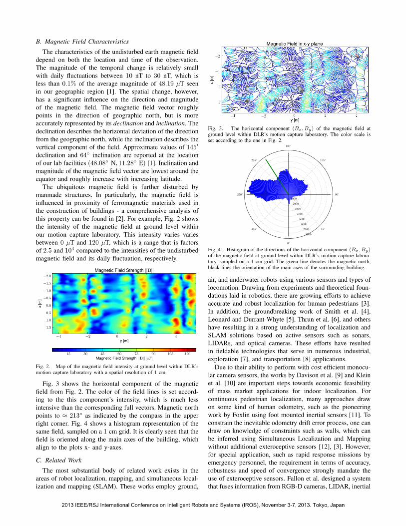
Fig. 3 shows the horizontal component of the magnetic

field from Fig. 2. The color of the field lines is set accord-

ing to the this component’s intensity, which is much less

intensive than the corresponding full vectors. Magnetic north

points to ≈ 213◦ as indicated by the compass in the upper

right corner. Fig. 4 shows a histogram representation of the

same field, sampled on a 1 cm grid. It is clearly seen that the

field is oriented along the main axes of the building, which

align to the plots x- and y-axes.

C. Related Work

The most substantial body of related work exists in the

areas of robot localization, mapping, and simultaneous local-

ization and mapping (SLAM). These works employ ground,

Fig. 3. The horizontal component (Bx, By) of the magnetic field atground level within DLR’s motion capture laboratory. The color scale isset according to the one in Fig. 2.

0◦

45◦

90◦

135◦

180◦

225◦

270◦

315◦

1000

2000

3000

4000

5000

6000

7000

8000

Fig. 4. Histogram of the directions of the horizontal component (Bx, By)of the magnetic field at ground level within DLR’s motion capture labora-tory, sampled on a 1 cm grid. The green line denotes the magnetic north,black lines the orientation of the main axes of the surrounding building.

air, and underwater robots using various sensors and types of

locomotion. Drawing from experiments and theoretical foun-

dations laid in robotics, there are growing efforts to achieve

accurate and robust localization for human pedestrians [3].

In addition, the groundbreaking work of Smith et al. [4],

Leonard and Durrant-Whyte [5], Thrun et al. [6], and others

have resulting in a strong understanding of localization and

SLAM solutions based on active sensors such as sonars,

LIDARs, and optical cameras. These efforts have resulted

in fieldable technologies that serve in numerous industrial,

exploration [7], and transportation [8] applications.

Due to their ability to perform with cost efficient monocu-

lar camera sensors, the works by Davison et al. [9] and Klein

et al. [10] are important steps towards economic feasibility

of mass market applications for indoor localization. For

continuous pedestrian localization, many approaches draw

on some kind of human odometry, such as the pioneering

work by Foxlin using foot mounted inertial sensors [11]. To

constrain the inevitable odometry drift error process, one can

draw on knowledge of constraints such as walls, which can

be inferred using Simultaneous Localization and Mapping

without additional exteroceptive sensors [12], [3]. However,

for special application, such as rapid response missions by

emergency personnel, the requirement in terms of accuracy,

robustness and speed of convergence strongly mandate the

use of exteroceptive sensors. Fallon et al. designed a system

that fuses information from RGB-D cameras, LIDAR, inertial

2013 IEEE/RSJ International Conference on Intelligent Robots and Systems (IROS), November 3-7, 2013. Tokyo, Japan

sensors, and barometric sensors [13]. This approach is able to

robustly localized in realtime for complex 6-DOF motion and

challenging trajectories on, for example, stairs and elevators.

Both academia and industry have recently shown great

interest in using the indoor magnetic field for localization.

This interest is motivated by recent findings on the informa-

tiveness of the magnetic field and the extremely low cost of

available sensors. Employing an iRobot Create mobile robot

platform equipped with a 3-axis magnetometer, Vallivaara et

al. were the first to generate geometrically consistent maps

of the magnetic field using SLAM [14]. Their work provides

significant inspiration for us, and we wish to extend their

results by investigating the magnetic field as close to the

ground as possible, where we expect a more temporally

stable and spatially informative field.

Le Grand and Thrun describe the use of magnetic sensors

in a smartphone to build a map of the magnetic field, which

could enable very economical mass market applications [15].

The authors use a similar algorithm as described in this work,

but measure the magnetic field at a higher height and do not

use odometry information. Additionally, no high precision

ground truth system was used for mapping or localization

reference. [16] and [17] propose leader-follower systems to

navigate groups of robots following a magnetic trajectory

measured by a leading robot. In [16] the authors use a 1D

map and a Kalman Filter for localization in a corridor. In [18]

the authors describe the historicals development and current

efforts to use large scale (natural) magnetic anomalies for

aircraft positioning. Among the most challenging application

of magnetic localization has been proposed and successfully

demonstrated by Moore et al. for perching aerial robots

on power lines [19]. In our own previous work, we have

analyzed the properties of the indoor magnetic fields with

respect to their potential use for localization of robots and

pedestrians [2]. These and other recent findings [20] by Kim

et al. have strongly motivated our research.

The idea of using foot mounted sensors for legged local-

ization is not limited to humans. In fact, there is much poten-

tial in using biped [21], [22], [23] or quadruped robots [24],

[25] to autonomously map the magnetic field of a 3D volume

space just above floor level. The resulting abundance of

information characterizing indoor environments will not only

serve as “infrastructure” for indoor pedestrian localization,

but also in progressing the state of motion planning and

control for legged robots [26]. Such databases can also serve

as replacements for more expensive localization methods

in the robotics community, both for basic research (e.g.,

gate analysis [27]) and for technology demonstrations (e.g.,

Robocup [28]).

II. PROBLEM STATEMENT

Consider the problem of localizing a subject in an indoor

environment, where the subject’s locomotion can be leg-

based (e.g., humans, biped robots, quadruped robots) or non-

legged-based (e.g., wheelchairs, Ackermann vehicles). We

focus on the two-dimensional localization problem, meaning

that the subject’s pose Pk at time step k ∈ Z≥0 is a

random variable1 that takes values from R2×S, i.e., the two-

dimensional Euclidean space with corresponding rotation.

For multiple pose hypotheses, we are interested in deter-

mining the hypothesis associated with the highest posterior

probability p(Pk|{ZU ZB}1:k), where the measurement se-

quence {ZU ZB}1:k is composed of odometry measurements

ZU1:k and magnetic field measurements ZB

1:k.

A. Indoor Magnetic Environment

Assuming a time-stationary indoor magnetic environment,

we model the a priori magnetic map B : R2 × S → R

3

as a vector field. More specifically, given a pose Pk within

the magnetic map’s domain, the map projects this pose to a

three dimensional vector B(Pk). Note that for any b ∈ R, the

magnetic field vector (0, 0, b) is parallel to the local gravity

vector.

B. Odometry and Magnetic Field Measurements

In this paper we rely on sources of odometry measure-

ments and co-located magnetic field measurements. Typi-

cally, the odometry is derived from inertial sensors for legged

locomotion and rotary encoders for wheeled locomotion.

Inertial sensors, in addition to providing odometry that is

differential, are also informative with respect to the subject’s

absolute attitude, as discussed in Section III-A.2. For sim-

plicity of notation, let ∆xUk ∈ R

2 and ∆ΘUk ∈ S denote

the measured change in translational and rotational position,

respectively, derived from the odometry measurement ZUk ,

for all times k.

By the term co-located, we mean that the magnetic field

measurement ZBk is taken at the pose Pk, for all times k. This

measurement is of vector form (ZBx

k ,ZBy

k ,ZBz

k ) ∈ R3, and

is implemented in various likelihood functions, as discussed

in Section III-A. We make the assumption that the sensor is

always close enough to the ground as to be subjected to the

ground-level magnetic field.

III. ALGORITHMS

We are interested in legged and non-legged locomotion

for which some form of odometry is available. Since this

odometry is affected by noise but is still informative, it

lends itself to serve in the prediction step of a Bayesian

filter. Following the prediction step, the resulting hypotheses

are evaluated in the update step of the filter. This eval-

uation considers how well the actual measurements from

the magnetic sensor match the magnetic map’s values at

the subject’s predicted pose. Since the likelihood functions

and probability distributions present in this Bayesian filter

are strongly multi-modal, we have chosen to use a particle

filter (also known as a sequential Monte Carlo filter) with

systematic resampling [29].

We assume the odometry is reasonably accurate from one

time step to the next, and we employ a proposal function that

randomly draws the next pose of a particle given its previous

pose, its error states of the odometry, and the odometry

measurement itself. The update step of the Bayesian filter

1We denote all random variables as bold faced capital letters.

2013 IEEE/RSJ International Conference on Intelligent Robots and Systems (IROS), November 3-7, 2013. Tokyo, Japan

then employs the measurement likelihood computed at the

particle’s pose given the magnetic field map. Specific to

legged localization using inertial sensors, we believe that

this proposal function is justified because, conditioned on

knowledge of the odometry’s error state such as angular drift,

prediction of the displacement vector between (legged) steps

is typically in the order of a centimeter [30]. This magnitude

is of the same order as the expected discrimination of the

magnetic field likelihood function per measurement [2].

A. Likelihood Functions

Consider a population of Np particles indexed by

i ∈ {1, . . . , Np}. Each particle has a corresponding pose

(x[i],Θ[i]) ∈ R2×S, odometry drift rate τ [i], and weight w[i],

where the pose is projected to a three dimensional magnetic

field vector B[i] := B(x[i],Θ[i]) = (B[i]x , B

[i]y , B

[i]z ) by the

magnetic map. We now discuss three likelihood function

variants, each of which uses the magnetic field measurement

ZBk to update the weights of the particles at time k. Note

that this update step of the particle filter is invoked only

for particles that reside within the mapped area, i.e., in the

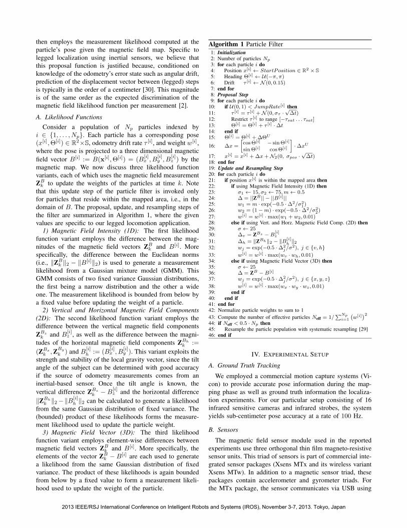
domain of B. The proposal, update, and resampling steps of

the filter are summarized in Algorithm 1, where the given

values are specific to our legged locomotion application.

1) Magnetic Field Intensity (1D): The first likelihood

function variant employs the difference between the mag-

nitudes of the magnetic field vectors ZBk and B[i]. More

specifically, the difference between the Euclidean norms

(i.e., ‖ZBk ‖2 − ‖B[i]‖2) is used to generate a measurement

likelihood from a Gaussian mixture model (GMM). This

GMM consists of two fixed variance Gaussian distributions,

the first being a narrow distribution and the other a wide

one. The measurement likelihood is bounded from below by

a fixed value before updating the weight of a particle.

2) Vertical and Horizontal Magnetic Field Components

(2D): The second likelihood function variant employs the

difference between the vertical magnetic field components

ZBz

k and B[i]z , as well as the difference between the magni-

tudes of the horizontal magnetic field components ZBh

k :=

(ZBx

k ,ZBy

k ) and B[i]h := (B

[i]x , B

[i]y ). This variant exploits the

strength and stability of the local gravity vector, since the tilt

angle of the subject can be determined with good accuracy

if the source of odometry measurements comes from an

inertial-based sensor. Once the tilt angle is known, the

vertical difference ZBz

k − B[i]z and the horizontal difference

‖ZBh

k ‖2−‖B[i]h ‖2 can be calculated to generate a likelihood

from the same Gaussian distribution of fixed variance. The

(bounded) product of these likelihoods forms the measure-

ment likelihood used to update the particle weight.

3) Magnetic Field Vector (3D): The third likelihood

function variant employs element-wise differences between

magnetic field vectors ZBk and B[i]. More specifically, the

elements of the vector ZBk − B[i] are each used to generate

a likelihood from the same Gaussian distribution of fixed

variance. The product of these likelihoods is again bounded

from below by a fixed value to form a measurement likeli-

hood used to update the weight of the particle.

Algorithm 1 Particle Filter

1: Initialization2: Number of particles Np

3: for each particle i do

4: Position x[i] ← StartPosition ∈ R2 × S

5: Heading Θ[i] ← U(−π, π)6: Drift τ [i] ← N (0, 0.15)7: end for

8: Proposal Step9: for each particle i do

10: if U(0, 1) < JumpRate[i] then

11: τ [i] = τ [i] +N (0, στ ·√∆t)

12: Restrict τ [i] to range [−τsat . . . τsat]13: Θ[i] = Θ[i] + τ [i] ·∆t14: end if

15: Θ[i] = Θ[i] +∆ΘU

16: ∆x =

[

cosΘ[i] − sinΘ[i]

sinΘ[i] cosΘ[i]

]

·∆xU

17: x[i] = x[i] +∆x+N2(0, σpos ·√∆t)

18: end for

19: Update and Resampling Step20: for each particle i do

21: if position x[i] is within the mapped area then

22: if using Magnetic Field Intensity (1D) then

23: σ1 ← 15, σ2 ← 75,m← 0.524: ∆ = ||ZB || − ||B[i]||25: w1 = m · exp(−0.5 ·∆2/σ2

1)26: w2 = (1−m) · exp(−0.5 ·∆2/σ2

2)27: w[i] = w[i] ·max(w1 + w2, 0.01)28: else if using Vert. and Horz. Magnetic Field Comp. (2D) then

29: σ ← 2530: ∆v = ZBz −B

[i]z

31: ∆h = ‖ZBh‖2 − ‖B[i]h‖2

32: wj = exp(−0.5 ·∆2j/σ

2), j ∈ {v, h}33: w[i] = w[i] ·max(wv · wh, 0.01)34: else if using Magnetic Field Vector (3D) then

35: σ ← 2536: ∆ = ZB −B[i]

37: wj = exp(−0.5 ·∆2j/σ

2), j ∈ {x, y, z}38: w[i] = w[i] ·max(wx · wy · wz , 0.01)39: end if

40: end if

41: end for

42: Normalize particle weights to sum to 1

43: Compute the number of effective particles Neff = 1/∑Np

i=1

(

w[i])2

44: if Neff < 0.5 ·Np then

45: Resample the particle population with systematic resampling [29]46: end if

IV. EXPERIMENTAL SETUP

A. Ground Truth Tracking

We employed a commercial motion capture systems (Vi-

con) to provide accurate pose information during the map-

ping phase as well as ground truth information the localiza-

tion experiments. For our particular setup consisting of 16

infrared sensitive cameras and infrared strobes, the system

yields sub-centimeter pose accuracy at a rate of 100 Hz.

B. Sensors

The magnetic field sensor module used in the reported

experiments use three orthogonal thin film magneto-resistive

sensor units. This triad of sensors is part of commercial inte-

grated sensor packages (Xsens MTx and its wireless variant

Xsens MTw). In addition to a magnetic sensor triad, these

packages contain accelerometer and gyrometer triads. For

the MTx package, the sensor communicates via USB using

2013 IEEE/RSJ International Conference on Intelligent Robots and Systems (IROS), November 3-7, 2013. Tokyo, Japan

a proprietary protocol for configuration and data logging;

the MTw uses a proprietary wireless communications link

operating in the 2.4 GHz ISM band. For the experiments,

both the odometry measurements ZUk and magnetic field

measurements ZBk are received at 100 Hz.

We used these sensors for the robotic magnetic mapping,

the non-legged localization, and the pedestrian localization.

For the robotic mapping, we mount the sensor on a wooden

beam that extended 0.75 m from the center of the robot.

The purpose of this beam is to separate the sensor from

the robot’s ferromagnetic components (e.g., bearings, steel

screws) and electromagnetic field generating devices (e.g.,

motors, motor drivers). We note that the distance of 0.75 m

was selected due to its sufficient separation yet reasonable

length with respect to the difficulty of positioning a long

“lever arm.”

C. Robotic Platform

In this work, we use an omnidirectional robot to perform

mapping as well as to analyze localization performance

for wheeled platforms. The robot is a modified version of

the commercially available Slider platform by Common-

place Robotics, see Fig. 5. The platform’s chassis made

of aluminum sheet metal, and its overall dimensions are

450 mm ×300 mm ×170 mm (length × width × height).

The drive system consists of two motor drivers with two

channels, four gearmotors with magnetic encoders, and four

Mecanum wheels of 150 mm diameter.

Fig. 5. Robotic platform with sensor arm in a calibrated projection of themagnetic field intensity.

The platform is fully holonomic and accepts forward,

lateral, and rotational velocity control inputs. The differential

measurements (∆xUk ,∆ΘU

k ) are derived from the odometry

measurements ZUk received from the four wheel encoders at

a rate of 50 Hz.

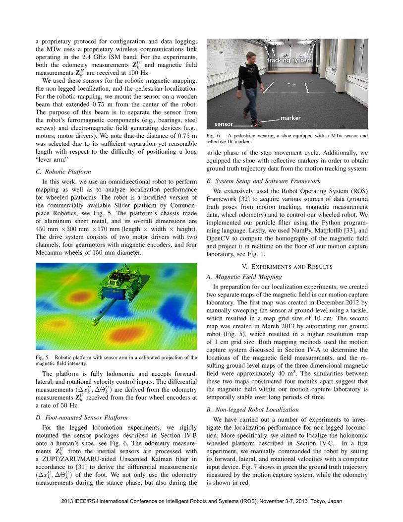
D. Foot-mounted Sensor Platform

For the legged locomotion experiments, we rigidly

mounted the sensor packages described in Section IV-B

onto a human’s shoe, see Fig. 6. The odometry measure-

ments ZUk from the inertial sensors are processed with

a ZUPT/ZARU/MARU-aided Unscented Kalman filter in

accordance to [31] to derive the differential measurements

(∆xUk ,∆ΘU

k ) of the foot. We not only use the odometry

measurements during the stance phase, but also during the

Fig. 6. A pedestrian wearing a shoe equipped with a MTw sensor andreflective IR markers.

stride phase of the step movement cycle. Additionally, we

equipped the shoe with reflective markers in order to obtain

ground truth trajectory data from the motion tracking system.

E. System Setup and Software Framework

We extensively used the Robot Operating System (ROS)

Framework [32] to acquire various sources of data (ground

truth poses from motion tracking, magnetic measurement

data, wheel odometry) and to control our wheeled robot. We

implemented our particle filter using the Python program-

ming language. Lastly, we used NumPy, Matplotlib [33], and

OpenCV to compute the homography of the magnetic field

and project it in realtime on the floor of our motion capture

laboratory, see Fig. 1.

V. EXPERIMENTS AND RESULTS

A. Magnetic Field Mapping

In preparation for our localization experiments, we created

two separate maps of the magnetic field in our motion capture

laboratory. The first map was created in December 2012 by

manually sweeping the sensor at ground-level using a tackle,

which resulted in a map grid size of 10 cm. The second

map was created in March 2013 by automating our ground

robot (Fig. 5), which resulted in a higher resolution map

of 1 cm grid size. Both mapping methods used the motion

capture system discussed in Section IV-A to determine the

locations of the magnetic field measurements, and the re-

sulting ground-level maps of the three dimensional magnetic

field were approximately 40 m2. The similarities between

these two maps constructed four months apart suggest that

the magnetic field within our motion capture laboratory is

temporally stable over long periods of time.

B. Non-legged Robot Localization

We have carried out a number of experiments to inves-

tigate the localization performance for non-legged locomo-

tion. More specifically, we aimed to localize the holonomic

wheeled platform described in Section IV-C. In a first

experiment, we manually commanded the robot by setting

its forward, lateral, and rotational velocities with a computer

input device. Fig. 7 shows in green the ground truth trajectory

measured by the motion capture system, while the odometry

is shown in red.

2013 IEEE/RSJ International Conference on Intelligent Robots and Systems (IROS), November 3-7, 2013. Tokyo, Japan

−4 −2 0 2 4 6 8x [m]

−6

−4

−2

0

2

4

6

y[m

]robot trajectory

lab boundaries

ground truth

odometry

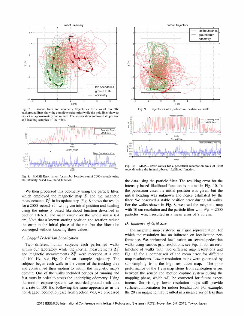
Fig. 7. Ground truth and odometry trajectories for a robot run. Thebackground lines show the complete trajectories while the bold lines show anextract of approximately one minute. The arrows show intermediate positionand heading samples of the robot.

0 500 1000 1500 2000time [s]

0

1

2

3

4

5

6

err

or

[m]

Robot Run

Odometry Error

MMSE Error

0 500 1000 1500 2000time [s]

0.00

0.05

0.10

0.15

0.20

0.25

err

or

[m]

Mean Error MMSE: 6.37 cm

Zoomed View

Fig. 8. MMSE Error values for a robot location run of 2000 seconds usingthe intensity-based likelihood function.

We then processed this odometry using the particle filter,

which employed the magnetic map B and the magnetic

measurements ZBk in its update step. Fig. 8 shows the results

for a 2000 seconds run with given initial position and heading

using the intensity based likelihood function described in

Section III-A.1. The mean error over the whole run is 6.4cm. Note that a known starting position and rotation reduce

the error in the initial phase of the run, but the filter also

converged without knowing these values.

C. Legged Pedestrian Localization

Two different human subjects each performed walks

within our laboratory while the inertial measurements ZUk

and magnetic measurements ZBk were recorded at a rate

of 100 Hz, see Fig. 9 for an example trajectory. The

subjects began each walk in the center of the tracking area

and constrained their motion to within the magnetic map’s

domain. One of the walks included periods of running and

fast turns in order to stress the underlying odometry. Using

the motion capture system, we recorded ground truth data

at a rate of 100 Hz. Following the same approach as in the

non-legged locomotion case from Section V-B, we processed

−4 −2 0 2 4 6 8x [m]

−6

−4

−2

0

2

4

6

y[m

]

human trajectory

lab boundaries

ground truth

odometry

Fig. 9. Trajectories of a pedestrian localization walk.

0 200 400 600 800 1000time [s]

0.00.51.01.52.02.53.03.54.0

err

or

[m]

Pedestrian Walk

Odometry Error

MMSE Error

0 200 400 600 800 1000time [s]

0.00

0.05

0.10

0.15

0.20

0.25

err

or

[m]

Mean Error MMSE: 7.95 cm

Zoomed View

Fig. 10. MMSE Error values for a pedestrian locomotion walk of 1020seconds using the intensity-based likelihood function.

the data using the particle filter. The resulting error for the

intensity-based likelihood function is plotted in Fig. 10. In

the pedestrian case, the initial position was given, but the

initial heading was unknown and hence estimated by the

filter. We observed a stable position error during all walks.

For the walks shown in Fig. 8, we used the magnetic map

with 10 cm resolution and the particle filter with NP = 2000particles, which resulted in a mean error of 7.95 cm.

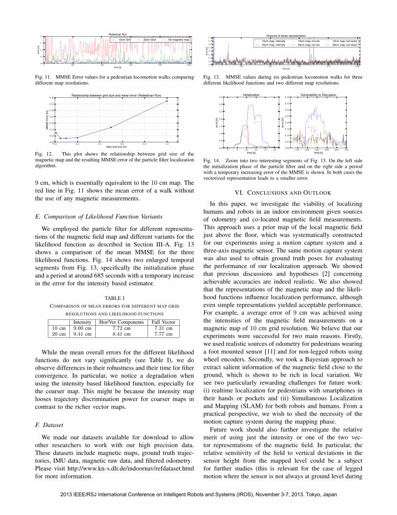
D. Influence of Grid Size

The magnetic map is stored in a grid representation, for

which the resolution has an influence on localization per-

formance. We performed localization on several pedestrian

walks using various grid resolutions, see Fig. 11 for an error

timeline of walks with two different map resolutions and

Fig. 12 for a comparison of the mean error for different

map resolutions. Lower resolution maps were generated by

sub-sampling from the high resolution map. The poor

performance of the 1 cm map stems from calibration errors

between the sensor and motion capture system during the

mapping phase, which will be corrected for future exper-

iments. Surprisingly, lower resolution maps still provide

sufficient information for indoor localization. For example,

the 20 cm magnetic map resulted in a mean error of less than

2013 IEEE/RSJ International Conference on Intelligent Robots and Systems (IROS), November 3-7, 2013. Tokyo, Japan

0 200 400 600 800 1000time [s]

0.0

0.5

1.0

1.5

2.0err

or

[m]

Pedestrian Run

10cm Grid 20cm Grid No magnetic map

Fig. 11. MMSE Error values for a pedestrian locomotion walks comparingdifferent map resolutions.

0.0 0.2 0.4 0.6 0.8 1.0Map grid size [m]

0.05

0.10

0.15

0.20

0.25

0.30

0.35

0.40

MM

SE

Err

or

[m]

Relationship between grid size and mean error (Pedestrian Run)

Fig. 12. This plot shows the relationship between grid size of themagnetic map and the resulting MMSE error of the particle filter localizationalgorithm.

9 cm, which is essentially equivalent to the 10 cm map. The

red line in Fig. 11 shows the mean error of a walk without

the use of any magnetic measurements.

E. Comparison of Likelihood Function Variants

We employed the particle filter for different representa-

tions of the magnetic field map and different variants for the

likelihood function as described in Section III-A. Fig. 13

shows a comparison of the mean MMSE for the three

likelihood functions. Fig. 14 shows two enlarged temporal

segments from Fig. 13, specifically the initialization phase

and a period at around 685 seconds with a temporary increase

in the error for the intensity based estimator.

TABLE I

COMPARISON OF MEAN ERRORS FOR DIFFERENT MAP GRID

RESOLUTIONS AND LIKELIHOOD FUNCTIONS

Intensity Hor/Ver Components Full Vector

10 cm 9.00 cm 7.72 cm 7.31 cm20 cm 9.41 cm 8.41 cm 7.77 cm

While the mean overall errors for the different likelihood

functions do not vary significantly (see Table I), we do

observe differences in their robustness and their time for filter

convergence. In particular, we notice a degradation when

using the intensity based likelihood function, especially for

the coarser map. This might be because the intensity map

looses trajectory discrimination power for coarser maps in

contrast to the richer vector maps.

F. Dataset

We made our datasets available for download to allow

other researchers to work with our high precision data.

These datasets include magnetic maps, ground truth trajec-

tories, IMU data, magnetic raw data, and filtered odometry.

Please visit http://www.kn-s.dlr.de/indoornav/refdataset.html

for more information.

0 200 400 600 800 1000time [s]

0.0

0.1

0.2

0.3

0.4

0.5

0.6

0.7

0.8

err

or

[m]

Influence of Vector representation

10cm map, intensity

20cm map, intensity

10cm map, hor/ver

20cm map, hor/ver

10cm map, full vector

20cm map, full vector

Fig. 13. MMSE values during six pedestrian locomotion walks for threedifferent likelihood functions and two different map resolutions.

6 8 10 12 14 16time [s]

0.0

0.5

1.0

1.5

2.0

2.5

3.0

3.5

err

or

[m]

Initialization

675 680 685 690 695 700time [s]

0.00

0.05

0.10

0.15

0.20

0.25

0.30

0.35

0.40

err

or

[m]

Vulnerability to Disruption

Fig. 14. Zoom into two interesting segments of Fig. 13. On the left sidethe initialization phase of the particle filter and on the right side a periodwith a temporary increasing error of the MMSE is shown. In both cases thevectorized representation leads to a smaller error.

VI. CONCLUSIONS AND OUTLOOK

In this paper, we investigate the viability of localizing

humans and robots in an indoor environment given sources

of odometry and co-located magnetic field measurements.

This approach uses a prior map of the local magnetic field

just above the floor, which was systematically constructed

for our experiments using a motion capture system and a

three-axis magnetic sensor. The same motion capture system

was also used to obtain ground truth poses for evaluating

the performance of our localization approach. We showed

that previous discussions and hypotheses [2] concerning

achievable accuracies are indeed realistic. We also showed

that the representations of the magnetic map and the likeli-

hood functions influence localization performance, although

even simple representations yielded acceptable performance.

For example, a average error of 9 cm was achieved using

the intensities of the magnetic field measurements on a

magnetic map of 10 cm grid resolution. We believe that our

experiments were successful for two main reasons. Firstly,

we used realistic sources of odometry for pedestrians wearing

a foot mounted sensor [11] and for non-legged robots using

wheel encoders. Secondly, we took a Bayesian approach to

extract salient information of the magnetic field close to the

ground, which is shown to be rich in local variation. We

see two particularly rewarding challenges for future work:

(i) realtime localization for pedestrians with smartphones in

their hands or pockets and (ii) Simultaneous Localization

and Mapping (SLAM) for both robots and humans. From a

practical perspective, we wish to shed the necessity of the

motion capture system during the mapping phase.

Future work should also further investigate the relative

merit of using just the intensity or one of the two vec-

tor representations of the magnetic field. In particular, the

relative sensitivity of the field to vertical deviations in the

sensor height from the mapped level could be a subject

for further studies (this is relevant for the case of legged

motion where the sensor is not always at ground level during

2013 IEEE/RSJ International Conference on Intelligent Robots and Systems (IROS), November 3-7, 2013. Tokyo, Japan

the entire stride). Data sets in different environments would

also provide further evidence whether the intensity map is

sufficient, especially when more events have been captured

where the estimated location suffers from error bursts.

We see a rich set of application scenarios for our proposed

approach of robot-based mapping and subsequent localiza-

tion for legged and non-legged locomotion. The mapping

phase could be assigned to floor cleaning or specialized

ground robots, and the resulting maps could then be shared

with other robotic or human users of the building. We believe

a “mild” form of SLAM is sufficient to keep maps current by

incorporating newly accessible regions or changes in the field

due to moved, added or removed steel structures. One should

note that a map of the magnetic field reveals potentially

less sensitive information about the indoor environment than

images; this property is relevant when addressing privacy

concerns. Furthermore, drawing on an additional source of

pose information from known magnetic field disturbances

should improve the continuity, integrity, and accuracy of

systems that use other maps and sensors.

REFERENCES

[1] LMU Geophysics, “Monthly magnetograms,” http://www.geophysik.uni-muenchen.de/observatory/geomagnetism/monthly-magnetograms,last accessed: August 7th, 2013.

[2] M. Angermann, M. Frassl, M. Doniec, B. Julian, and P. Robertson,“Characterization of the indoor magnetic field for applications in lo-calization and mapping,” in Indoor Positioning and Indoor Navigation

(IPIN), 2012 International Conference on, nov. 2012.[3] M. Angermann and P. Robertson, “FootSLAM: Pedestrian simul-

taneous localization and mapping without exteroceptive sensors -hitchhiking on human perception and cognition,” Proceedings of the

IEEE, vol. 100, no. Special Centennial Issue, pp. 1840–1848, 13.[4] R. Smith, M. Self, and P. Cheeseman, “Autonomous robot vehicles.”

New York, NY, USA: Springer-Verlag New York, Inc., 1990, ch.Estimating uncertain spatial relationships in robotics, pp. 167–193.

[5] J. Leonard and H. Durrant-Whyte, “Simultaneous map building andlocalization for an autonomous mobile robot,” in Intelligent Robots

and Systems ’91. ’Intelligence for Mechanical Systems, Proceedings

IROS ’91. IEEE/RSJ International Workshop on, Nov 1991.[6] M. Montemerlo, S. Thrun, D. Koller, and B. Wegbreit, “Fastslam:

a factored solution to the simultaneous localization and mappingproblem,” in Eighteenth national conference on Artificial intelligence.Menlo Park, CA, USA: American Association for Artificial Intelli-gence, 2002, pp. 593–598.

[7] R. M. Eustice, H. Singh, J. J. Leonard, and M. R. Walter, “Visuallymapping the RMS Titanic: Conservative covariance estimates forSLAM information filters,” Int. J. Rob. Res., vol. 25, no. 12, pp. 1223–1242, Dec. 2006.

[8] C. Urmson and W. Whittaker, “Self-driving cars and the urbanchallenge,” Intelligent Systems, IEEE, vol. 23, no. 2, pp. 66–68, march-april 2008.

[9] A. Davison, I. Reid, N. Molton, and O. Stasse, “Monoslam: Real-timesingle camera slam,” Pattern Analysis and Machine Intelligence, IEEE

Transactions on, vol. 29, no. 6, pp. 1052–1067, june 2007.[10] G. Klein and D. Murray, “Parallel tracking and mapping for small ar

workspaces,” in Mixed and Augmented Reality, 2007. ISMAR 2007. 6th

IEEE and ACM International Symposium on, nov. 2007, pp. 225–234.[11] E. Foxlin, “Pedestrian tracking with shoe-mounted inertial sensors,”

Computer Graphics and Applications, IEEE, vol. 25, no. 6, pp. 38–46, nov.-dec. 2005.

[12] P. Robertson, M. Angermann, and B. Krach, “Simultaneous localiza-tion and mapping for pedestrians using only foot-mounted inertialsensors,” in Proceedings of the 11th international conference on

Ubiquitous computing (Ubicomp), 2009.[13] M. Fallon, H. Johannsson, J. Brookshire, S. Teller, and J. Leonard,

“Sensor fusion for flexible human-portable building-scale mapping,” inIntelligent Robots and Systems (IROS), 2012 IEEE/RSJ International

Conference on, oct. 2012, pp. 4405–4412.

[14] J. Haverinen and A. Kemppainen, “A global self-localization techniqueutilizing local anomalies of the ambient magnetic field,” in Robotics

and Automation, 2009. ICRA ’09. IEEE International Conference on,may 2009.

[15] E. Le Grand and S. Thrun, “3-axis magnetic field mapping and fusionfor indoor localization,” in Multisensor Fusion and Integration for

Intelligent Systems (MFI), 2012 IEEE Conference on, sept. 2012.[16] B. Gozick, K. Subbu, R. Dantu, and T. Maeshiro, “Magnetic maps for

indoor navigation,” Instrumentation and Measurement, IEEE Transac-

tions on, vol. 60, no. 12, pp. 3883 –3891, dec. 2011.[17] T. Riehle, S. Anderson, P. Lichter, J. Condon, S. Sheikh, and D. Hedin,

“Indoor waypoint navigation via magnetic anomalies,” in Engineering

in Medicine and Biology Society,EMBC, 2011 Annual International

Conference of the IEEE, sept 2011.[18] F. Goldenberg, “Geomagnetic navigation beyond the magnetic com-

pass,” in IEEE/ION Position Location And Navigation Symposium

(PLANS), 2006, april 2006.[19] J. Moore and R. Tedrake, “Magnetic localization for perching UAVs on

powerlines,” in Intelligent Robots and Systems (IROS), 2011 IEEE/RSJ

International Conference on, sept. 2011.[20] S.-E. Kim, Y. Kim, J. Yoon, and E. S. Kim, “Indoor positioning system

using geomagnetic anomalies for smartphones,” in Indoor Positioning

and Indoor Navigation (IPIN), 2012 International Conference on,2012, pp. 1–5.

[21] Y. Sakagami, R. Watanabe, C. Aoyama, S. Matsunaga, N. Higaki, andK. Fujimura, “The intelligent ASIMO: System overview and integra-tion,” in Intelligent Robots and Systems, 2002. IEEE/RSJ International

Conference on, vol. 3. IEEE, 2002, pp. 2478–2483.[22] K. Kaneko, K. Harada, F. Kanehiro, G. Miyamori, and K. Akachi,

“Humanoid robot HRP-3,” in Intelligent Robots and Systems, 2008.

IROS 2008. IEEE/RSJ International Conference on. IEEE, 2008, pp.2471–2478.

[23] K. Kaneko, F. Kanehiro, M. Morisawa, K. Akachi, G. Miyamori,A. Hayashi, and N. Kanehira, “Humanoid robot hrp-4-humanoidrobotics platform with lightweight and slim body,” in Intelligent

Robots and Systems (IROS), 2011 IEEE/RSJ International Conference

on. IEEE, 2011, pp. 4400–4407.[24] A. Shkolnik, M. Levashov, I. R. Manchester, and R. Tedrake, “Bound-

ing on rough terrain with the littledog robot,” The International

Journal of Robotics Research, vol. 30, no. 2, pp. 192–215, 2011.[25] M. Raibert, K. Blankespoor, G. Nelson, R. Playter, et al., “Bigdog,

the rough–terrain quadruped robot,” in Proceedings of the 17th World

Congress, 2008, pp. 10 823–10 825.[26] J. Chestnutt, M. Lau, G. Cheung, J. Kuffner, J. Hodgins, and

T. Kanade, “Footstep planning for the Honda ASIMO humanoid,” inRobotics and Automation, 2005. ICRA 2005. Proceedings of the 2005

IEEE International Conference on. IEEE, 2005, pp. 629–634.[27] N. Kohl and P. Stone, “Policy gradient reinforcement learning for

fast quadrupedal locomotion,” in Robotics and Automation, 2004.

Proceedings. ICRA’04. 2004 IEEE International Conference on, vol. 3.IEEE, 2004, pp. 2619–2624.

[28] H. Kitano, M. Asada, Y. Kuniyoshi, I. Noda, and E. Osawa, “Robocup:The robot world cup initiative,” in Proceedings of the first international

conference on Autonomous agents. ACM, 1997, pp. 340–347.[29] M. Sanjeev Arulampalam, S. Maskell, N. Gordon, and T. Clapp, “A

tutorial on particle filters for online nonlinear/non-gaussian bayesiantracking,” Signal Processing, IEEE Transactions on, vol. 50, no. 2, pp.174–188, 2002.

[30] M. Angermann, P. Robertson, T. Kemptner, and M. Khider, “A highprecision reference data set for pedestrian navigation using foot-mounted inertial sensors,” in Indoor Positioning and Indoor Naviga-

tion (IPIN), 2010 International Conference on, sept. 2010.[31] F. Zampella, M. Khider, P. Robertson, and A. Jimenez, “Unscented

kalman filter and magnetic angular rate update (MARU) for animproved pedestrian dead-reckoning,” in IEEE/ION Position Location

And Navigation Symposium (PLANS), 2012, april 2012.[32] M. Quigley, K. Conley, B. P. Gerkey, J. Faust, T. Foote, J. Leibs,

R. Wheeler, and A. Y. Ng, “ROS: an open-source robot operatingsystem,” in ICRA Workshop on Open Source Software, Kobe, Japan,2009.

[33] J. Hunter, “Matplotlib: A 2D graphics environment,” Computing in

Science Engineering, vol. 9, no. 3, pp. 90–95, may-june 2009.

2013 IEEE/RSJ International Conference on Intelligent Robots and Systems (IROS), November 3-7, 2013. Tokyo, Japan