Embed Size (px)
Citation preview

Department of Physics and Astronomy
Magnetic and Magneto-Optical
Properties of Doped Oxides
Mohammed S. Alqahtani
Thesis submitted to the University of Sheffield for the degree of
Doctor of Philosophy
October 2012

Acknowledgments
It has been a real privilege to study and research as a participant in the
magnetic oxide semiconductors group at the University of Sheffield. I wish to express
my great gratitude and sincere appreciation to my principle supervisor, Professor
Gillian Gehring. I am really in debt to her for her inspiring guidance, overwhelming
support and fruitful discussion throughout the development of this thesis.
Thanks are also due to my Co-advisor, Mark Fox and to Dr. Harry Blythe for
their assistance and valuable suggestions throughout the various stages of the
experimental parts of the work.
I extend a special thanks to my colleagues Qi Feng, David Score, Ali Hakimi,
Minju Ying, Hasan Albargi and Wala Dizayee for their encouragement, and for the
fantastic time I have had.
Special thanks to my parents who have been always a great support to me
since my childhood. Also, I would like to thank all my brothers and sisters, my friends
Dr. Mohammed Alshorman and Dr. Saad Alqahtani for all their support. Finally, I
wish to thank my son Yasser and my daughter Lana for their love and patient.
Last of all, but no means the least; I am thankful to the chairmen/women and
members of the department of physics and Astronomy in the University of Sheffield
for their help and encouragement.
Mohammed Alqahtani
Sheffield, October 2012.

Abstract
This thesis describes the growth, structural characterisation, magnetic and magneto-
optics properties of lanthanum strontium manganite (LSMO), GdMnO3 and transition
metal (TM)-doped In2O3 thin films grown under different conditions. The SrTiO3 has
been chosen as a substrate because its structure is suitable to grow epitaxial LSMO
and GdMnO3 films. However, the absorption of SrTiO3 above its band gap at about
3.26 eV is actually a limitation in this study. The LSMO films with 30% Sr, grown on
both SrTiO3 and sapphire substrates, exhibit a high Curie temperature (Tc) of 340 K.
The magnetic circular dichroism (MCD) intensity follows the magnetisation for
LSMO on sapphire; however, the measurements on SrTiO3 were dominated by the
birefringence and magneto-optical properties of the substrate. In the GdMnO3 thin
films, there are two well-known features in the optical spectrum; the charge transfer
transition between Mn d states at 2 eV and the band edge transition from the oxygen p
band to d states at about 3 eV; these are observed in the MCD. This has been
measured at remanence as well as in a magnetic field. The optical absorption at 3 eV
is much stronger than at 2 eV, however, the MCD is considerably stronger at 2 eV.
The MCD at 2 eV correlates well with the Mn spin ordering and it is very notable that
the same structure appears in this spectrum, as is seen in LaMnO3. The results of the
investigations of Co and Fe-doped In2O3 thin films show that TM ions in the films are
TM2+
and substituted for In3+
. The room temperature ferromagnetism observed in
TM-doped In2O3 is due to the polarised electrons in localised donor states associated
with oxygen vacancies. The formation of Fe3O4 nanoparticles in some Fe-doped films
is due the fact that TM-doped In2O3 thin films are extremely sensitive to the growth
method and processing condition. However, the origin of the magnetisation in these
films is due to both the Fe-doped host matrix and also to the nanoparticles of Fe3O4.

Publications
Gillian A. Gehring, Harry J. Blythe, Qi Feng, David S. Score, Abbas Mokhtari,
Marzook Alshammari, Mohammed S. Al Qahtani and A. Mark Fox, Using Magnetic
and optical methods to determine the size and characteristics of nanoparticles
embedded in oxide semiconductors, IEEE Transactions on Magnetics, vol. 46, issue 6,
pp. 1784-1786.(2010).
A. M. H. R. Hakimi, M. G. Blamire, S. M. Heald, M. S. Alshammari, M. S.
Alqahtani, D. S. Score, H. J. Blythe, A. M. Fox and G. A. Gehring, Donor band
ferromagnetism in cobalt-doped indium oxide, Physical Review B 84 (8), 085201
(2011).
F.-X. Jiang, X.-H. Xu, J. Zhang, X.-C. Fan, H.-S. Wu, M. Alshammari, Q. Feng, H. J.
Blythe, D. S. Score, K. Addison, M. Al-Qahtani and G. A. Gehring, Room
temperature ferromagnetism in metallic and insulating (In1-xFex)2O3 thin films,
Journal of Applied Physics 109 (5), 053907-053907 (2011).
Mohammed S. Al Qahtani, Marzook Alshammari, H.J Blythe, A.M. Fox,
G.A.Gehring,N. Andreev, V. Chichkov, and Ya, Mukovskii, Magnetic and Optical
properties of strained films of multiferroic GdMnO3, Journal of Physics (accepted
2012).
Marzook S. Alshammari, Mohammed S Alqahtani, AM Fox, HJ Blythe, A. M. H. R.
Hakimi,SM HealdS. Alfahad, M. Alotibi, A. Alyamani, GA Gehring, Magnetic,
Transport, Optical and Magneto-optical investigations of In2O3 containing Fe3O4
nanoparticles, (prepared for publication).
David S. Score, James R. Neal, Anthony J. Behan, Abbas Mokhtari, Feng Qi,
Marzook Alshammari, Mohammed S. Al Qahtani, Harry J. Blythe, A. Mark Fox,
Roy W. Chantrell, Steve M Heald, Stefan T. Ochsenbein and Daniel R. Gamelin,
Gillian A. Gehring, Enhanced magnetism in ZnCoO by exchange coupling to Co
nanoparticles ,(prepared for publication).

Conferences
M. Alshammari, Mohammed S. Al Qahtani, Qi Feng, H.J. Blythe, D.S. Score, K.
Addison, A.M. Fox, G.A. Gehring , Feng-Xian Jiang, Xiao-Hong Xu, Jun Zhang,
Xiao-Chen Fan, Hai-Shun Wu, Influence of oxygen pressure on the magnetic and
transport properties of Fe-doped In2O3 thin films, Condensed Matter and Materials
Physics CMMP09, at the University of Warwick, 2009, Dec. 15-17, UK.
Mohammed S. Al Qahtani, Marzook Alshammari, H.J Blythe, A.M. Fox,
G.A.Gehring,N. Andreev, V. Chichkov, and Ya, Mukovskii, Magnetic and Optical
properties of strained films of multiferroic GdMnO3, Condensed Matter and Material
Physics Conference (CMMP) 2010, University of Warwick, 2010, Dec. 14-16, UK.

v
Contents
Acknowledgments........................................................................................................... i
Abstract .......................................................................................................................... ii
Publications .................................................................................................................. iii
Chapter 1- Introduction and Thesis Structure
1.1 Introduction .............................................................................................................. 1
1.2 Thesis Structure ....................................................................................................... 3
1.3 References ................................................................................................................ 5
Chapter 2- Theoretical Background
2.1 Introduction .............................................................................................................. 8
2.2 Magnetic Moment of Electron in a Free Ion ............................................................ 8
2.3 Magnetisation in Solids.......................................................................................... 12
2.4 Diamagnetism ........................................................................................................ 13
2.5 Paramagnetism ....................................................................................................... 14
2.6 Ferromagnetism ..................................................................................................... 16
2.7 Anti-Ferromagnetism ............................................................................................. 20
2.8 Exchange Interaction in Magnetic Systems ........................................................... 21
2.8.1 Direct Exchange Interaction ........................................................................... 21
2.8.2 Indirect Interactions ........................................................................................ 21
I Super-Exchange ................................................................................................. 22
II Double Exchange Interaction ........................................................................... 23
III RKKY Interaction ........................................................................................... 24
2.9 A Brief History of Oxide Thin Films ..................................................................... 25
2.10 References ............................................................................................................ 30

vi
Chapter 3- Experimental Methods
3.1 Introduction: ........................................................................................................... 33
3.2 Target and Film Preparation: ................................................................................. 33
3.3 Pulsed Laser Deposition ........................................................................................ 34
3.3.1 Excimer Laser ................................................................................................. 34
3.3.2 Basics Excimer Laser ...................................................................................... 35
3.3.3 Mechanisms of Pulsed Laser Deposition ........................................................ 37
3.4 Growth of Thin Films and PLD System ................................................................ 39
3.5 Measuring Film Thickness- Dektak Surface Profiler ............................................ 42
3.6 Measuring Magnetisation – SQUID Magnetometer .............................................. 45
3.6.1 SQUID Fundamentals ..................................................................................... 45
3.6.2 Sample Handling and SQUID Operation ........................................................ 47
3.7 Magneto-Optics Basics .......................................................................................... 51
3.8 Magneto-Optics Set-up and Principles of the Technique ...................................... 53
3.9 Optical Transmission and Reflection Techniques ................................................. 57
3.10 Thin Films Samples Investigated ......................................................................... 60
3.11 References .......................................................................................................... 63
Chapter 4- Lanthanum Strontium Manganite (LSMO)
4.1 Introduction: ........................................................................................................... 67
4.2 Literature Review on LSMO ................................................................................. 68
4.3 Experiment Results and Discussion ....................................................................... 79
4.3.1 The Dependence of Magnetic Properties on Oxygen Pressure and Type of
Substrate ................................................................................................................... 81
4.3.2 Dependence of Magnetic Properties on Film Thickness ................................ 86
4.3.3 Dependence of Magnetic Properties on Annealing ........................................ 89
4.3.4 Magneto-Optical Properties of LSMO Thin Films ......................................... 92

vii
4.4 Summary and Conclusions .................................................................................... 99
4.5 References ............................................................................................................ 101
Chapter 5- Multiferroic Manganite GdMnO3
5.1 Introduction .......................................................................................................... 106
5.2 Literature Review on the Multiferroic, Gadolinium Manganite (GdMnO3)........ 107
5.3 Experimental Results and Discussion .................................................................. 113
5.3.1 Magnetic Measurements ............................................................................... 114
5.3.2 Optical Measurements .................................................................................. 119
5.4 Summary and Conclusions .................................................................................. 128
5.5 References ............................................................................................................ 129
Chapter 6- Strontium Titanate STO Substrates
6.1 Introduction .......................................................................................................... 132
6.2 Literature on Optical and Magneto-Optical properties of STO Substrates.......... 132
6.3 Experiment Results and Discussion ..................................................................... 137
6.4 Summary and Conclusions .................................................................................. 149
6.5 References ............................................................................................................ 150
Chapter 7- Transition Metal (TM) Doped In2O3
7.1 Introduction .......................................................................................................... 152
7.2 Literature Review on TM Doped In2O3 ............................................................... 152
7.3 Experiment Result and Discussion ...................................................................... 157
7.3.1 Co Doped In2O3 ............................................................................................ 157
7.3.2 Fe Doped In2O3 ............................................................................................. 164
7.4 Summary and Conclusions .................................................................................. 179
7.5 References ............................................................................................................ 181

viii
Chapter 8- Conclusions and Future Work
8.1 Conclusions .......................................................................................................... 186
8.1.1 LSMO Thin Films ......................................................................................... 186
8.1.2 GdMnO3 Thin Films ..................................................................................... 188
8.1.3 Co and Fe-Doped In2O3 Thin Films.............................................................. 189
8.2 Future Work ......................................................................................................... 190
8.3 Reference ............................................................................................................. 192
Appendix A
Chapter 6 – Appendix ................................................................................................ 194
References .................................................................................................................. 197
Chapter 1 - Introduction
1
Chapter 1
Introduction and Thesis Structure
1.1 Introduction
A spintronics or spin device electronics, where the spin of electrons in addition
to their electrical charge is used to encode information, is an emerging technology
that replaces conventional semiconductor-based electronic devices [1-2]. The concept
of a spintronic device relies on a source of spin-polarised currents, and so researchers
have shown intense interest in materials that have the largest possible spin
polarisations of the conduction electrons at the Fermi level. Of most interest for
research, are materials which display metallic characteristics for the majority-spin
electrons, while the Fermi energy falls in a gap in the density of states for the
minority-spin electrons. This behaviour is known as half-metallic ferromagnetism and
was predicted to occur in oxides [3-4]. There is particular interest in the half-metallic
material systems which include doped manganites, double perovskites and magnetite.
All of them show Curie temperatures above room temperature, meaning they are well-
suited for the purposes of spintronics [2, 5]. Amongst a wide range of Perovskite-type
of manganites, (La0.7 Sr0.3) MnO3 (LSMO) is expected to display a nearly complete
spin polarisation at the Fermi level. The potential has been observed for LSMO thin
films to perform well in spintronic devices [6-7].
The field of oxide electronics has expanded exponentially since the 1990’s,
due to the discovery of high-Tc superconductors and with the progress in thin film
technology. Oxides are representative of strongly correlated electronic systems;

Chapter 1 - Introduction
2
therefore they have versatile physical properties. Different degrees of freedom are
present and different ordering phenomena occur within the same materials and result
in phenomena including superconductivity and ferromagnetism [2].
Semiconducting indium oxide (In2O3) is in the focus for current research and
thought to be an ideal material for dilute magnetic semiconductors (DMS) when
doped with transitional metal (TM) ions. Room temperature ferromagnetism has been
reported for all 3d TM (V, Cr, Fe, Cu, Ni and Co) doped In2O3 [8-20]. Indium oxide is
a cubic structure with 80 atoms per unit cell. It has a wide band-gap energy (3.75 eV),
large carrier density when doped with Sn and is transparent in the visible region. All
these properties make In2O3 well-suited for the purposes of device applications [21-
23].
Multiferroic oxides are another possible candidate for spintronics device
applications [24-25]. These oxides have the property of two or more ferroic order
parameters co-existing in one single phase. The majority of the multiferroic transition
metal oxides display antiferromagnetic properties, so research is required to find those
oxides that display ferromagnetic properties [26-27]. However, some success has been
observed in applications of multiferroics. They have been used as thin film barriers in
spin filter tunnel junctions and in semiconductor devices as electrodes [2, 25].
The subject of this thesis is the study of the magnetic and magneto-optic
properties of LSMO, multiferroic GdMnO3 and TM-doped In2O3 thin films.
Chapter 1 - Introduction
3
1.2 Thesis Structure
This thesis consists of eight chapters, chapter one is the introduction of
the thesis and chapter two provides basic concepts and background information
on magnetisation and magneto-optics. A discussion of the exchange interaction
and a history on oxide thin films are introduced in this chapter.
Chapter three describes the experimental techniques used in this thesis. It
also gives some background information beyond the techniques and describes
how the work was carried out.
Chapter four describes the experimental investigation of the magnetic and
magneto-optics properties of LSMO thin films. The effect of growth conditions,
substrate, film thickness and annealing on magnetic and magneto-optics
properties is introduced. In addition, a literature review on LSMO is given in this
chapter.
Chapter five describes the experimental investigation of the magnetic and
magneto-optics properties of multiferroic GdMnO3 thin films. The role of strain
in these films is discussed in this chapter. It also gives a literature review on
multiferroic manganite GdMnO3.
Chapter six describes the experimental investigation of the optical and
magneto- optical properties of the STO substrate. The film grown on an STO
substrate exhibited an anomalous magnet-optics behaviour due to the
birefringence of the STO substrate. The influence of birefringence on the
magneto-optics data taken using the Sato method is given in this chapter.
Chapter seven describes the experimental investigation of the magnetic
and magneto-optics properties of Co and Fe doped In2O3 thin films. The
influence of TM concentration, growth conditions, annealing and adding Sn on

Chapter 1 - Introduction
4
the magnetic and magneto-optics properties is introduced in this chapter. The
contribution of TM ions to the magnetisation is explored in order to determine
the origin of the ferromagnetism and a new method is established to estimate the
contribution of Co and Fe ions in In2O3 system. This chapter also provides an
introduction and a literature review of TM-doped In2O3.
Chapter eight is a summary of the experimental results. Proposals for
future work and projects are also discussed.

Chapter 1 - Introduction
5
1.3 References
1. G. A. Prinz, Science 282 (5394), 1660-1663 (1998).
2. M. Opel, Journal of Physics D-Applied Physics 45 (3) (2012).
3. A. Yanase and K. Siratori, Journal of the Physical Society of Japan 53 (1),
312-317 (1984).
4. R. A. Degroot, F. M. Mueller, P. G. Vanengen and K. H. J. Buschow, Physical
Review Letters 50 (25), 2024-2027 (1983).
5. J. M. D. Coey and C. L. Chien, Mrs Bulletin 28 (10), 720-724 (2003).
6. H. L. Liu, K. S. Lu, M. X. Kuo, L. Uba, S. Uba, L. M. Wang and H. T. Jeng,
Journal of Applied Physics 99 (4), 043908-043907 (2006).
7. T. K. Nath, J. R. Neal and G. A. Gehring, Journal of Applied Physics 105 (7),
07D709-703 (2009).
8. D. Berardan, E. Guilmeau and D. Pelloquin, Journal of Magnetism and
Magnetic Materials 320 (6), 983-989 (2008).
9. L. M. Huang, C. M. Araujo and R. Ahuja, Epl 87 (2) (2009).
10. H. W. Ho, B. C. Zhao, B. Xia, S. L. Huang, J. G. Tao, A. C. H. Huan and L.
Wang, Journal of Physics-Condensed Matter 20 (47) (2008).
11. Sub, iacute, G. as, J. Stankiewicz, F. Villuendas, M. Lozano, P. a, Garc and J.
a, Physical Review B 79 (9), 094118 (2009).
12. J. Philip, A. Punnoose, B. I. Kim, K. M. Reddy, S. Layne, J. O. Holmes, B.
Satpati, P. R. LeClair, T. S. Santos and J. S. Moodera, Nat Mater 5 (4), 298-
304 (2006).
13. G. Z. Xing, J. B. Yi, D. D. Wang, L. Liao, T. Yu, Z. X. Shen, C. H. A. Huan,
T. C. Sum, J. Ding and T. Wu, Physical Review B 79 (17), 174406 (2009).
Chapter 1 - Introduction
6
14. R. P. Panguluri, P. Kharel, C. Sudakar, R. Naik, R. Suryanarayanan, V. M.
Naik, A. G. Petukhov, B. Nadgorny and G. Lawes, Physical Review B 79
(16), 165208 (2009).
15. Y. K. Yoo, Q. Xue, H.-C. Lee, S. Cheng, X. D. Xiang, G. F. Dionne, S. Xu, J.
He, Y. S. Chu, S. D. Preite, S. E. Lofland and I. Takeuchi, Applied Physics
Letters 86 (4), 042506-042503 (2005).
16. O. D. Jayakumar, I. K. Gopalakrishnan, S. K. Kulshreshtha, A. Gupta, K. V.
Rao, D. V. Louzguine-Luzgin, A. Inoue, P. A. Glans, J. H. Guo, K. Samanta,
M. K. Singh and R. S. Katiyar, Applied Physics Letters 91 (5), 052504-
052503 (2007).
17. D. Chu, Y.-P. Zeng, D. Jiang and Z. Ren, Applied Physics Letters 91 (26),
262503-262503 (2007).
18. P. F. Xing, Y. X. Chen, S.-S. Yan, G. L. Liu, L. M. Mei, K. Wang, X. D. Han
and Z. Zhang, Applied Physics Letters 92 (2), 022513-022513 (2008).
19. X.-H. Xu, F.-X. Jiang, J. Zhang, X.-C. Fan, H.-S. Wu and G. A. Gehring,
Applied Physics Letters 94 (21), 212510-212513 (2009).
20. F.-X. Jiang, X.-H. Xu, J. Zhang, H.-S. Wu and G. A. Gehring, Applied
Surface Science 255 (6), 3655-3658 (2009).
21. H. Kim, M. Osofsky, M. M. Miller, S. B. Qadri, R. C. Y. Auyeung and A.
Pique, Applied Physics Letters 100 (3), 032404-032403 (2012).
22. J.-H. Lee, S.-Y. Lee and B.-O. Park, Materials Science and Engineering: B
127 (2–3), 267-271 (2006).
23. C. Nunes de Carvalho, G. Lavareda, A. Amaral, O. Conde and A. R. Ramos,
Journal of Non-Crystalline Solids 352 (23–25), 2315-2318 (2006).
24. M. Fiebig, Journal of Physics D-Applied Physics 38 (8), R123-R152 (2005).

Chapter 1 - Introduction
7
25. N. A. Spaldin, S.-W. Cheong and R. Ramesh, Physics Today 63 (10), 38-43
(2010).
26. T. Kimura, S. Kawamoto, I. Yamada, M. Azuma, M. Takano and Y. Tokura,
Physical Review B 67 (18) (2003).
27. N. A. Spaldin and M. Fiebig, Science 309 (5733), 391-392 (2005).

Chapter 2 – Theoretical Background
8
Chapter 2
Theoretical Background
2.1 Introduction
This chapter will provide a brief discussion of the concepts of magnetism and
the various possible exchange interactions. It will also provide a history of the
investigation of oxide materials that relate to the topics covered in this thesis. The
introduction to the concepts of magnetisation was obtained by referring to the
following text books: “Magnetic Materials Fundamentals and Device Applications”
by N.A.Saldin [1], “Introduction to Solid States Physics” by C. Kittel [2], “Physics of
Magnetism and Magnetic Materials” by K.H.J.Buschow and F.R.D.Boer [3],
“ Magnetism and magnetic materials” by J.M.D.Coey [4].
2.2 Magnetic Moment of Electron in a Free Ion
Magnetic moment is the fundamental object in magnetism. From elementary
physics, the current I circulating in a loop of area A produces a magnetic moment
given by:
2.1
The direction of is normal to the plane of the loop and such that the current
flows counter-clockwise relative to an observer, standing along as shown in
fig.2.1.

Chapter 2 – Theoretical Background
9
A magnetic dipole moment is so called because it behaves similarly to an
electric dipole which consists of one negative charge and one positive charge
separated by a small distance. In a similar way, the movement of the electron around
the nucleus produces a magnetic moment given by:
= ( , 2.2
where, is the current due to the circulation of the electric charge (e) in a circular
orbit with period T around the nucleus. The orbital angular momentum of the electron
is given by:
L= , 2.3
where is the radius of the circular orbit, m is the mass of the electron and is the
angular velocity. Hence, the magnetic moment of the electron in terms of its angular
momentum is given by:
Nucleus
𝜇𝑚
𝑙 -e
Figure (2.1): the electron moves in circular orbit where the magnetic moment
and the quantised angular momentum are oppositely directed.
Chapter 2 – Theoretical Background
10
(
2.4
From quantum theory the angular momentum of an orbital electron is determined by
the orbital quantum number as:
2.5
Substituting the value of from eqn. 2.5 into eqn. 2.4 gives:
2.6
Eqn. (2.6) shows that an electron in an atom can take only certain specified values of
magnetic moment (quantised) depending on the values. The component of the
orbital angular momentum along the applied magnetic field direction is given by ,
where is the orbital magnetic quantum number. The quantity
is called
the Bohr magneton which equals 9.27 10-24
J/T.
To fully specify the state of an electron in the atom, a fundamental concept
needs to be introduced; this is the spin of the electron. By an analogy with the orbital
magnetic moment, it might be expected that the spin magnetic moment is given by:
2.7
But, in fact, this is incorrect and the situation for the spin angular momentum
is different because twice as much moment is created by spin angular momentum than
for orbital angular momentum. Therefore the spin magnetic moment is given by:
, 2.8
where, the factor g is called the g-factor of the electron or the Landé splitting
factor. This was originally introduced by Landé to explain the anomalous Zeeman
effect and latter theories have justified the assumption theoretically. By taking g=2 the
spin magnetic moment along the field direction is one Bohr magneton for a single
electron.

Chapter 2 – Theoretical Background
11
Similarly to the electron, the nucleus has its own spin associated with its
angular momentum. The mass of the nucleus is of the order of 2000 times the mass of
electron and hence the magnetic moment associated with the nuclear spin can be
ignored since it is very small.
The total spin angular momentum, , and the total orbital angular
momentum, , of the electrons are combined to determine the total angular
momentum , , as follows:
∑ , ∑ and 2.9
This type of coupling is referred to L-S coupling (Russell-Saunders coupling).
In light atoms the coupling between the individual spins to give and the individual
orbital angular momenta to give is stronger than spin-orbit coupling giving .
However, there is also j-j coupling for the heavy atoms where the spin-orbit coupling
dominates. In this case, the spin and orbital angular momenta of individual electrons
couple to give the total angular momenta per electron which interact via electron
distributions to form the resultant total angular momentum.
The total magnetic moment, is not collinear with but makes
an angle, , with, , and precesses around it. Therefore, the magnetic moment and
then the magnetic properties are determined by:
, 2.10
where, is called the Landé g-factor and is given by:
( ( (
( 2.11

Chapter 2 – Theoretical Background
12
The atomic magnetic moment( ) determines the magnetisation of the system. The
magnetisation of a material is expressed in terms of density of net magnetic
moment .
2.3 Magnetisation in Solids
In solids, the magnetism of the material is defined as the sum of the magnetic
moments per unit volume as:
∑
2.12
When an external magnetic field (H) is applied to a material, the relationship
between H and the magnetic induction (B) is given by:
( , 2.13
where, Hm-1
is the magnetic permeability in free space and
M is the magnetisation of the material. The properties of the material are defined by
the way in which M or B varies with the applied magnetic field H. The ability of a
material to become magnetised is called magnetic susceptibility ( ) which is defined
in low field as the ratio between M and H:
2.14
The permeable of the material to the magnetic field is called permeability ( ) and
given by:
2.15
The relative permeability of the material ( is defined as the ratio of and :

Chapter 2 – Theoretical Background
13
2.16
The values of the magnetic susceptibility ( ) and the relative permeability
( can be used to classify magnetic materials. The materials with negative
susceptibility are defined as diamagnetic whereas if the susceptibility and the
permeability are small and positive the materials are known as paramagnetic. As for
paramagnetic materials, ferromagnetic materials have a positive susceptibility and
permeability, but much larger values.
2.4 Diamagnetism
The susceptibility of diamagnetic materials is negative as has been mentioned
in sect. (2.3). The application of a magnetic field to the diamagnetic material leads to
the induced magnetic moment being directed in the opposite direction of the applied
magnetic field as shown in fig.2.2; and this type of magnetism is found in all matter.
The materials in which diamagnetic is observed consist of atoms that have no net
magnetic moment, because they have filled electron shells. The noble gases, NaCl and
Al2O3 are examples of materials that show this type of magnetism. The classical
Langevin theory and quantum theory give the same result for the diamagnetic
susceptibility which is given by:
⟨ ⟩
, 2.17
where, Z is the number of electrons, e is the electron charge; N is the number
of atoms per unit volume, is the electron mass and ⟨ ⟩ is the average value of
all occupied orbital radii. It is clear from eqns. 2.17 that the diamagnetic susceptibility
is negative and temperature independent.

Chapter 2 – Theoretical Background
14
2.5 Paramagnetism
Paramagnetic materials have a net magnetic moment due to the unpaired
electron in the partially-filled orbitals. The magnetic moments on neighbouring atoms
in paramagnetic materials are non-interacts and the temperature causes random
orientation of these moments. The application of a magnetic field aligns the magnetic
moments partially toward the field direction. At low field, the magnetisation of
paramagnetic materials increases as the magnetic field is increased and the
paramagnetic susceptibility is temperature dependent as shown in fig. 2.3. The
paramagnetic susceptibility is given by Curie’s law as:
, 2.18
Figure (2.2): The diamagnetic magnetisation and susceptibility are negative and independent
of temperature.
𝜒 𝑠𝑙𝑜𝑝𝑒 <
H
M

Chapter 2 – Theoretical Background
15
where, √ ( , is the Curie constant and is Boltzmann’s
constant.
In fact Curie’s law is modified if moments interact ferromagnetically to give the
Cure-Weiss law which is given by:
2.19
The paramagnetic materials follow the Cure-Weiss law until a critical
temperature ( below which the material becomes ferromagnetic. The magnetic
moment of the paramagnetic ions can be calculated using equation (2.10). The
calculated and experimental values of the magnetic moment are in agreement for most
paramagnetic ions. However for transition-metals this agreement does not work,
unless the orbital angular momentum of the electrons is completely ignored as shown
Figure (2.3): a) The paramagnetic magnetisation and susceptibility are positive b) The
paramagnetic susceptibility is temperature dependent.
M
a
H
𝜒
b
T
𝜒 ∝
𝜒 𝑠𝑙𝑜𝑝𝑒 >

Chapter 2 – Theoretical Background
16
in Table (2.1) for some transition-metal ions used in this thesis. This phenomenon is
called quenching of the orbital angular momentum where the electric fields generated
by the surrounding ions in the solid force the orbitals to be coupled strongly to the
crystal lattice. As a result, the orbitals are prevented turning toward the field and then
the magnetic moment is determined by electron spin only.
Removed by the
author for copyright reasons
Table (2.1): Calculated and measured effective magnetic moment for some transition-metal
ions [1-2].
2.6 Ferromagnetism
Ferromagnetic materials are magnetic materials that exhibit spontaneous
magnetisation and a magnetic ordering temperature. The presence of ferromagnetic
behaviour in common materials (iron, cobalt, nickel) is due to the atoms containing
unfilled orbits. Most of the ferromagnetic metals have 4s and 3d partially filled bands.
The d bands are relatively flat and the mobility of the d band electrons is low
(localized) whereas s bands are parabolic structure and the mobility of s band

Chapter 2 – Theoretical Background
17
electrons are high (delocalized). The exchange interaction between electrons induces
the electrons bands splitting. This leads to an imbalance between the density of spin-
up (majority) and spin-down (minority) of 3d electrons as shown in fig. 2.4, which
give rise to the magnetisation. However, application of an external magnetic field can
enhance or weaken the band splitting and thus changes the magnetisation. A weaker
exchange interaction in a 4s band causes a balance in the distribution of 4s spin-up
and spin-down electrons. Therefore, the 3d band is responsible for the magnetism in
the ferromagnetic metals [5-8].
Figure (2.4): Diagram showing the band structure of the ferromagnetic metals. The 3d band
is split into spin-up (majority) and spin-down (minority) causes a net magnetic moment per
atom. The Fermi level EF is represented by the dashed line.
E
4S
3d
EF
𝑑𝑁
𝑑𝐸
Majority spin Minority spin

Chapter 2 – Theoretical Background
18
Ferromagnetic materials obey the Curie-Weiss law above the critical
temperature called Curie temperature where above this temperature the
ferromagnetic materials become paramagnetic. The susceptibility of the ferromagnetic
material at > is given by:
2.20
The susceptibility has a positive value at > but at T equal to the
susceptibility becomes infinite, which corresponds to the spontaneous order phase.
This means that the ferromagnetic materials have spontaneous magnetisation even in
the absence of the external magnetic field. However, a ferromagnetic material has
zero initial magnetisation which indicates that ferromagnetic material consists of
small regions called domains and the magnetic dipoles are aligned parallel in each
domain. In the absence of an external magnetic field the magnetisation in different
domains has a different orientation and then the total magnetisation average is zero.
The process of magnetisation causes magnetic dipoles of all domains to orient in the
same direction. The magnetisation of a ferromagnet is a complex function of the
applied magnetic field and depends on the material’s past history, as shown in fig. 2.5.
The graph of magnetisation (M) versus magnetic field (H) shown in fig. 2.5 is known
as a hysteresis loop. In an applied magnetic field, the magnetisation of the system
increases as the field is increased until it reaches a maximum at the saturation
magnetisation (Ms). When the magnetic field is reduced to zero after saturation, the
magnetisation decreases to a certain value (Mr) called the remnant magnetisation. The
reversed magnetic field required to reduce the magnetisation to zero is called the
coercivity (HC). The magnetisation and the susceptibility of ferromagnetic materials
are temperature dependent as shown in fig.2.6. The saturation magnetisation reaches
its maximum at absolute zero and vanishes above the Curie temperature ( ).

Chapter 2 – Theoretical Background
19
Figure (2.5): Variation of the magnetisation with magnetic field (hysteresis loop) for a
ferromagnetic material. Ms denotes the saturation magnetisation, HC the coercive field and
Mr the remnant magnetisation.
Figure (2.6): a) The magnetisation as a function of temperature for a ferromagnetic material.
b) The inverse susceptibility as a function of temperature for a ferromagnetic material.
a
TC
Magnetisation
Temperature
b
𝜒
TC T
-1.0 -0.5 0.0 0.5 1.0-15
-10
-5
0
5
10
15
Mr
Hc
Ms
Magnetisation x
10
-5(e
mu)
Magnetic field (T)
Chapter 2 – Theoretical Background
20
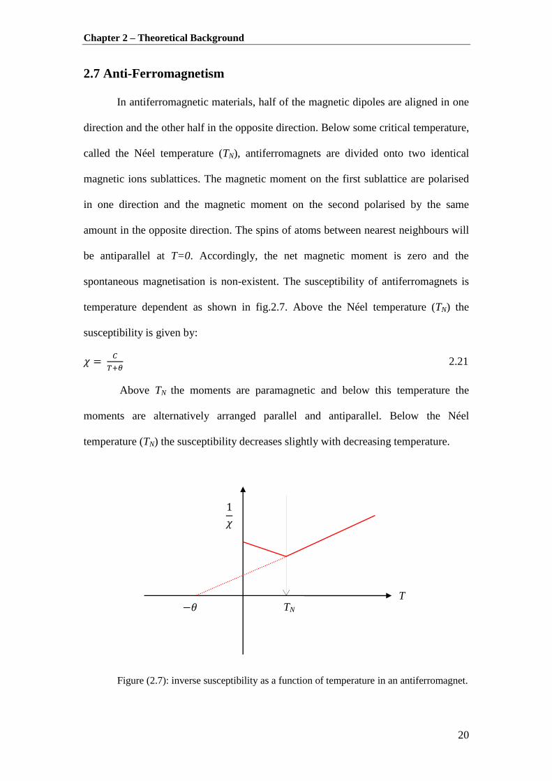
2.7 Anti-Ferromagnetism
In antiferromagnetic materials, half of the magnetic dipoles are aligned in one
direction and the other half in the opposite direction. Below some critical temperature,
called the Néel temperature (TN), antiferromagnets are divided onto two identical
magnetic ions sublattices. The magnetic moment on the first sublattice are polarised
in one direction and the magnetic moment on the second polarised by the same
amount in the opposite direction. The spins of atoms between nearest neighbours will
be antiparallel at T=0. Accordingly, the net magnetic moment is zero and the
spontaneous magnetisation is non-existent. The susceptibility of antiferromagnets is
temperature dependent as shown in fig.2.7. Above the Néel temperature (TN) the
susceptibility is given by:
2.21
Above TN the moments are paramagnetic and below this temperature the
moments are alternatively arranged parallel and antiparallel. Below the Néel
temperature (TN) the susceptibility decreases slightly with decreasing temperature.
Figure (2.7): inverse susceptibility as a function of temperature in an antiferromagnet.
TN 𝜃
𝜒
T

Chapter 2 – Theoretical Background
21
2.8 Exchange Interaction in Magnetic Systems
The magnetic and electrical behaviour depends on the interaction between the
different atoms. There are many different exchange interactions that have been used
to explain ferromagnetism in the magnetic system. These interactions can be divided
into categories of direct and indirect interactions.
2.8.1 Direct Exchange Interaction
Direct exchange interaction occurs between spin on ions which are close
enough to have sufficient overlap of their wave functions. If two single free atoms
exist beside one another, with their respective lobes of charge density that correspond
to different states. These lobes typically form an overlap region of charge density that
will contribute to both atoms. The Pauli exclusion principle requires that no single
electron state is occupied twice. Therefore, the electrons are then required to possess
opposite spins. This gives rise to an antiparallel alignment and therefore the direct
exchange interaction is antiferromagnetic. The direct exchange sign depends
principally on the interatomic spacing and band occupancy with ferromagnetic
exchange favoured at a larger spacing [4].
2.8.2 Indirect Interactions
It is not possible for coupling to take place through direct exchange if the ions,
on which the magnetic moments are located, are situated with excessive space
between them. The exchange must therefore take place in an indirect manner such as
super-exchange, double exchange and RKKY exchange.

Chapter 2 – Theoretical Background
22
I Super-Exchange
Super-exchange is a coupling that occurs between two nearest-neighbour
cations through a shared non-magnetic ion (e.g. oxygen). The transition metal oxides
are a good illustration of the super-exchange interaction. In transition metal oxides the
3d-orbitals are hybridized with the 2p-O orbitals. Virtual hopping of O-2p electrons to
the overlapping transition metal (TM) orbitals leads to excited states which can result
in a reduction of the total energy of the system. The strength and the sign of the super-
exchange interaction depend on the occupancy and orbital degeneracy of the 3d states.
This can leads to antiferromagnetic or ferromagnetic behaviour as summarized below
for La3+
Mn3+
as an example [9].
1- The super-exchange interaction that occurs between the half-filled d-shell of
Mn3+
ions and the fully occupied O-2p electrons is antiferromagnetic as shown in
fig. (2.8 a). Since the hopping of the two O-2p electrons will reduce the system
energy if the spins of Mn3+
ions on the either side of the anion (oxygen) are of
opposite spin.
2- The super-exchange interaction is ferromagnetic if the two nearest-neighbour
Mn3+
ions are connected at 90 degree to the oxygen ion. Since the hopping of the
two O-2p electrons will reduce the system energy if the spin of Mn3+
core spins
are parallel as shown in fig.2.8 b

Chapter 2 – Theoretical Background
23
Removed by the
author for copyright reasons
Figure (2.8): super-exchange interaction between the eg orbital of two Mn3+
ions via the O-2p
for LaMnO3. Dependent on the occupation with electrons, the resulting interaction is a)
antiferromagnetic b) ferromagnetic. Adapted from ref. [9].
II Double Exchange Interaction
The double exchange interaction (DE) was proposed by Zener [10]. It is a type
of interaction that occurs indirectly between the spins of magnetic ions and needs
mixed valence. The DE is responsible for ferromagnetism in the mixed-valence
perrovskite manganites where the extra electron of the Mn3+
ion travel back and forth
between Mn3+
and Mn4+
ions and its spin is coupled with those of both ion cores. The

Chapter 2 – Theoretical Background
24
difference DE and super-exchange interaction is that the super-exchange interaction
occurs between two atoms with the same valence (number of electrons). More details
regarding DE are given in section 4.2 of chapter 4.
III RKKY Interaction
The Ruderman-Kittel-Kasuya-Yosida (RKKY) interaction [11] describes the
magnetic interaction between localized d or f electron spins (magnetic ion) and the
delocalized conduction band electrons (sp-band). Due to the direct exchange
interaction the spin of one magnetic ion interacts with the close conduction electron.
This conduction electron is then magnetised and acts as an effective field which
influences the polarisation of the nearby magnetic ions. The polarisation decays in an
oscillatory manner as the distance from the magnetic ion is increased. Consequently, a
second magnetic ion can then couple parallel to the first magnetic ion, but only if
there is a small separation of the magnetic moments. This model is efficient when a
high concentration of delocalized carriers is present in the host material. The RKKY
mechanism illustrates an interaction with much longer range than direct interaction,
but the mechanism can vary widely in terms of strength, with minor changes in the
magnetic moment separation.

Chapter 2 – Theoretical Background
25
2.9 A Brief History of Oxide Thin Films
The history of oxide thin films was intensely influenced by the development of
the suitable deposition techniques [9]. Several techniques were used to grow epitaxial
oxide thin films; these include techniques such as sputtering, molecular beam epitaxy
(MBE) etc. However, no other growth method had such a high impact as the
development of the novel pulsed laser deposition (PLD) technique in the late 1980s
[9, 12-13]. Since the discovery of tunnelling magnetoresistance (TMR) on tunnel
junctions based on manganese peroviskite oxides [14-15], the interest has increased
rapidly for the application of oxides in the field of spintronics. Among oxides
materials that have been produced very large TMR are the half-metallic oxides [16-
17]. Half-metallic behaviour in double- exchange oxides was predicted for Fe3O4 in
1984 [18], CrO2 in 1986 [19], and Manganites in 1996 [20]. Mixed-valence
manganites, such as La0.67Sr0.33MnO3 (LSMO), are DE ferromagnets with a maximum
Curie temperature TC of 360 K [21]. Part of this thesis focuses on LSMO and a
literature review of LSMO is presented in section 4.2 of chapter 4.
The discovery of ferromagnetism in Diluted magnetic semiconductors (DMSs)
greatly increased research activity in this field. DMSs are a solid-solution of a non-
magnetic semiconductor and magnetic element, as shown in fig. 2.9. In diluted
magnetic semiconductors (DMSs) transition metals with unfilled d shells (Sc,Ti,V ,Cr
,Mn ,Fe,Co,Ni and Cu) and rare earth elements with unfilled f shells (e.g Eu,Gd and
Er) have been used as magnetic elements. The content of magnetic element in a
DMSs ranges from a few percent to several tens of percent [22-23]. The interaction
between magnetic ions is critical where the absence of this interaction leads to
paramagnetism of the DMSs. The ferromagnetism of a DMS can arise under certain
condition such as changes in the density of free carriers, which can lead to exchange
Chapter 2 – Theoretical Background
26
interaction between magnetic ions. In a DMSs the delocalised valence band holes and
conduction band electrons interact with the magnetic moment associated with the
magnetic atoms [22].
Removed by the
author for copyright reasons
Figure (2.9): Two types of semiconductors a) a magnetic semiconductor b) a diluted magnetic
semiconductors (DMS). Adapted from ref.[24].
A significant contribution to the research on DMSs was made by Slyn’ko et al
in 1980s [25]. These workers, were the first to discover Fe magnetic ordered cluster in
InSe and CdTe. The low Curie temperature and the difficulty in doping II-VI- based
DMSs n-type and p-type made these materials less attractive for applications [22].
A breakthrough in the field of DMSs was in 1989 by Munekata et al [26] who

Chapter 2 – Theoretical Background
27
succeeded in doping a considerable amount of Mn into InAs using MBE. However,
the Curie temperature TC for this material was very low at about 7.5 K [26-27].
DMSs have been studied in depth both experimentally and theoretically. Dietl
et al [28] calculated the Curie temperature for various wide band gap semiconductors
as shown in fig. 2.10. It was predicted that the Curie temperature could exceed room
temperature in p-type semiconductor-based- DMSs. This theoretical study encouraged
several groups to work in this field. In addition to this, reports of room temperature
ferromagnetism in Co-doped TiO2 films [29] have encouraged experimental studies
and intensive experimental work has begun on oxide- based DMSs.
Removed by the
author for copyright reasons
Figure (2.10): Calculated values of the Curie temperature TC for various p-type semi-
conductors containing 5% of Mn atoms and 3.5 x10²⁰
holes/ cm3 [28].
Coey et al, considered a model assuming indirect exchange via shallow donors
[30]. According to this model, high TC required hybridization and charge transfer
from the impurity band to the unoccupied 3d states at the Fermi level as shown in
fig.2.11. Consequently, on passing along the 3d series of metals there are two regions

Chapter 2 – Theoretical Background
28
in which a high TC is expected; one of these occurs when the states cross the
Fermi level in the impurity band at the beginning of the series (fig. 2.11 a), and the
other occurs when the states cross the Fermi level in the impurity band at the end
of the series (fig.2.11 c).
Removed by the
author for copyright reasons
Figure (2.11): Schematic band structure of an oxide containing 3d impurity and spin-split
donor impurity band. The position of the 3d level that leads to a high TC is shown in (a, c).
b) Shows the position of the 3d level that leads to a lower TC. Adapted from ref. [30].
In order to examine the Coey model, thin films of ZnO all doped with 5% of
each of the 3d TM element (Sc, Ti, V, Cr, Mn, Fe, Co, Ni, Cu and, Zn) were grown
using PLD [30]. The results were in agreement with the model where the highest
room temperature magnetisations (in /cation) occured for Co, Fe, Ni, V, Ti and Sc,
respectively. The magnetisation (in /cation) is near zero for Cr, Mn and Cu.
However a significant room temperature magnetisation was reported [31-32] for a low
concentration of Mn ( 2-3%) doped ZnO films.
Chapter 2 – Theoretical Background
29
Recently, In2O3-based DMSs have attracted great attention as candidates for
room temperature ferromagnetism and are expected to have the potential to widen the
range of application due to the wide band-gap (3.75 eV) and are transparent in the
visible region [33]. Part of this thesis focuses on TM doped In2O3 and a literature
review of In2O3 is presented in section 7.2 of chapter 7.
More recently, a renewed interest in multiferroic materials in the form of thin
films has provided novel opportunities for oxides in spintronics. Multiferroics brings
novel physics phenomena and offers possibilities for new device functions due to the
coexistence of several ferroic orders such as ferroelectrcity and ferromagnetism [34].
Part of this thesis focuses on multiferroics and a literature review on multiferroics is
presented in section 5.2 of chapter 5.

Chapter 2 – Theoretical Background
30
2.10 References
1. N. A. Spaldin, Magnetic materials : fundamentals and device applications.
(Cambridge University Press, Cambridge, Uk ; New York, 2003).
2. C. Kittel, Introduction to solid state physics, 6th ed. (Wiley, New York, 1986).
3. K. H. J. Buschow and F. R. d. Boer, Physics of magnetism and magnetic
materials. (Kluwer Academic/Plenum Publishers, New York, 2003).
4. J. M. D. Coey, Magnetism and magnetic materials. (Cambridge University
Press, Cambridge, 2010).
5. D. G. Pettifor, Journal of Magnetism and Magnetic Materials 15-8 (JAN-),
847-852 (1980).
6. F. J. Himpsel, J. E. Ortega, G. J. Mankey and R. F. Willis, Advances in
Physics 47 (4), 511-597 (1998).
7. O. Gunnarsson, Journal of Physics F-Metal Physics 6 (4), 587-606 (1976).
8. J. F. Janak, Phys. Rev. B 16 (1), 255-262 (1977).
9. M. Opel, J. Phys. D-Appl. Phys. 45 (3) (2012).
10. C. Zener, Physical Review 82 (3), 403-405 (1951).
11. K. Yosida, Theory of magnetism. (Springer, Berlin ; New York, 1996).
12. H. M. Christen and G. Eres, Journal of Physics: Condensed Matter 20 (26),
264005 (2008).
13. L. W. Martin, Y. H. Chu and R. Ramesh, Materials Science and Engineering:
R: Reports 68 (4–6), 89-133 (2010).
14. M. Bibes and A. Barthelemy, IEEE Trans. Electron Devices 54 (5), 1003-1023
(2007).
15. Y. Lu, X. W. Li, G. Q. Gong, G. Xiao, A. Gupta, P. Lecoeur, J. Z. Sun, Y. Y.
Wang and V. P. Dravid, Phys. Rev. B 54 (12), R8357-R8360 (1996).

Chapter 2 – Theoretical Background
31
16. J. M. D. Coey and M. Venkatesan, J. Appl. Phys. 91 (10), 8345-8350 (2002).
17. J. M. D. Coey and S. Sanvito, J. Phys. D-Appl. Phys. 37 (7), 988-993 (2004).
18. A. Yanase and K. Siratori, J. Phys. Soc. Jpn. 53 (1), 312-317 (1984).
19. K. Schwarz, Journal of Physics F-Metal Physics 16 (9), L211-L215 (1986).
20. W. E. Pickett and D. J. Singh, Phys. Rev. B 53 (3), 1146-1160 (1996).
21. M. Imada, A. Fujimori and Y. Tokura, Rev. Mod. Phys. 70 (4), 1039-1263
(1998).
22. C. Liu, F. Yun and H. Morkoc, J. Mater. Sci.-Mater. Electron. 16 (9), 555-597
(2005).
23. G. V. Lashkarev, M. V. Radchenko, V. A. Karpina and V. I. Sichkovskyi,
Low Temp. Phys. 33 (2-3), 165-173 (2007).
24. H. Ohno, Science 281 (5379), 951-956 (1998).
25. V. V. Slynko and R. D. Ivanchuk, Ukr Fiz Zh+ 26 (2), 221-223 (1981).
26. H. Munekata, H. Ohno, S. von Molnar, A. Segmüller, L. L. Chang and L.
Esaki, Physical Review Letters 63 (17), 1849-1852 (1989).
27. K. Kagami, M. Takahashi, C. Yasuda and K. Kubo, Sci. Technol. Adv. Mater.
7 (1), 31-41 (2006).
28. T. Dietl, H. Ohno, F. Matsukura, J. Cibert and D. Ferrand, Science 287 (5455),
1019-1022 (2000).
29. Y. Matsumoto, M. Murakami, T. Shono, T. Hasegawa, T. Fukumura, M.
Kawasaki, P. Ahmet, T. Chikyow, S. Koshihara and H. Koinuma, Science 291
(5505), 854-856 (2001).
30. J. M. D. Coey, M. Venkatesan and C. B. Fitzgerald, Nat. Mater. 4 (2), 173-179
(2005).

Chapter 2 – Theoretical Background
32
31. M. Ivill, S. J. Pearton, D. P. Norton, J. Kelly and A. F. Hebard, J. Appl. Phys.
97 (5), 053904-053905 (2005).
32. P. Sharma, A. Gupta, K. V. Rao, F. J. Owens, R. Sharma, R. Ahuja, J. M. O.
Guillen, B. Johansson and G. A. Gehring, Nat Mater 2 (10), 673-677 (2003).
33. M. Venkatesan, R. D. Gunning, P. Stamenov and J. M. D. Coey, J. Appl.
Phys. 103 (7) (2008).
34. M. Bibes and A. Barthelemy, Nat. Mater. 7 (6), 425-426 (2008).

Chapter 3 - Experimental Set-up and Techniques
33
Chapter 3
Experimental Methods
3.1 Introduction
This chapter describes the experimental techniques, the sample preparation
and the characterisation measurements that have been the basis of this work. This will
involve the procedure for production and measurement of thin film’s thicknesses and
magnetic moments. This chapter will also provide a brief discussion on the basics of
the magneto-optics. It also describes the procedure for the measurement of the optical
and magneto-optical properties of the samples. The introduction to the magneto-optics
basics was obtained by referring to the following text books: “ Optical properties of
Solids” by A.M.Fox [1] and “Magnetic Materials Fundamentals and Device
Applications” by N.A.Spaldin [2].
3.2 Target and Film Preparation
Our ultimate aim was the growth of thin films. These films were ablated from
bulk targets using an excimer (XeCl); a technique known as pulsed laser deposition
(PLD). The targets were prepared before ablation; we now describe the method of
production. Stoichiometric amounts of the appropriate powders were weighed-out
using an accurate balance. The requisite amounts of powders was mixed together and
ground for 20 minutes in a mortar and pestle. This powder-mix was then annealed for
about eight hours in air in a furnace. The resulting powders were then re-ground and
re-fired at a higher temperature for the same length of time in order to optimise the

Chapter 3 - Experimental Set-up and Techniques
34
reaction of components to form the oxide compound. After the final anneal, sufficient
powder was placed in a commercial die of internal diameter 25 mm and pressed to
25000 kPa in vacuo to yield a pellet of about 5 mm thickness. This pellet was then
sintered again at increasing temperatures for various lengths of time. The final result
was a high density, a smooth-surfaced target, which was then subsequently used in the
laser ablation chamber.
3.3 Pulsed Laser Deposition
There are several alternative techniques that can be employed to produce high-
quality thin films and multilayers. Examples of these techniques are molecular-beam
epitaxy (MBE), sputtering [3-4] or metal organic chemical vapour deposition
(MOCVD), aqueous deposition and (PLD) [3, 5-6] . The PLD technique is now
widely used for the growth of metal oxide films. It is a suitable laboratory technique
for growing high- quality epitaxial layers directly from a ceramic target. PLD was
first developed by Cheung et al and has been mostly employed for sequential
deposition of compound semiconductors [7].
3.3.1 Excimer Laser
In discussing different kinds of lasers, identification is made by the material
undergoing the laser process. There are four categories of lasing materials: solid, gas,
liquid, and semiconductor [8]. According to these categories there are many different
types of laser available for many different uses and the excimer laser is a pertinent
example [9]. The effect of laser beam on a target is affected by three variables: power,
spot size, and time. The change of energy with power and time are proportional while
that of spot size is an inverse square.

Chapter 3 - Experimental Set-up and Techniques
35
A pulsed laser, of which an excimer laser is an example, delivers its energy in the
form of a single pulse or train of pulses [8]. Laser light emitted from a standard device
is generally characterized in terms of power, in units of watts. The energy in Joules is
defined as a power in watts multiplied by the time (sec). Pulsating laser energy is
calculated for each pulse as in CW. The average power (Pavg) produced by a train of
pulses is determined by multiplying the pulse power (p) by the pulse repetition rate (f)
and the pulse width (Δt) [10-11]as following:
pavg (Watt) = p (W) f (Hz) Δt (sec) 3.1
3.3.2 Basics Excimer Laser
The word excimer is a contraction of the two words, excited dimer. The
excimer laser was invented in 1970 by Nikolai Basov. In an excimer laser the lowest
energy state of the molecules is not bound but repulsive. The excited state is a bound
state which is induced by an electrical discharge or high-energy electron beam. The
excimer laser action can then be produced on the transition between the upper state
(bound state) and the lower state ( free state) [8-9].
An excimer laser typically uses an inert gas such as argon (Ar), krypton (Kr)
or xenon (Xe) to combine, in the excited state, with a halogen atom such as fluorine
(F) or chlorine (Cl) to form a rare-gas-halide excimer [9]. The typical laser used for
growth is the excimer with KrF at the wavelength of 248nm, XeCl at 308 nm or ArF
at 193 nm, all values lying in the ultra violet UV. Most materials used in film growth
exhibit strong absorption in the region of the laser wavelength range from 200 nm to
400 nm [3, 12-14]. Fig.3.1 shows the potential energy diagram as a function of atomic
Chapter 3 - Experimental Set-up and Techniques
36
separation for the production of an excimer . This formation is created by the
collision of an excited atom with B or by the collision of a positive or negative ion
and [15]. Here, the potential is always repulsive in the lowest energy state,
whilst the excited states exhibit a minimum energy at one separation. Consequently,
the population inversion is easily achieved due to the low population in the ground
state. Furthermore, even when lasing commences, the ground state population remains
low because the ground state is inherently unstable [8].
Removed by the
author for copyright reasons
Figure (3.1): Potential energy curves showing the formation of the excimer [8].
The fundamental, avalanche electric discharge circuit layout is illustrated by
fig.3.2. This comprises a pair of electrodes, a storage capacitor and inductive coils.
The plasma tube contains the gaseous medium at high pressure. In order to produce
the laser, a high potential is applied to charge the storage capacitor to approximately
40 kV. Subsequently the thyratron switch is fired, meaning the energy is transferred to

Chapter 3 - Experimental Set-up and Techniques
37
the peaking capacitors over about 100 ns. The energy is then transferred to the
discharge area as the peaking capacitors become fully charged, and the time duration
of this transfer is 20-50 ns [12, 16].
Removed by the
author for copyright reasons
Figure (3.2): Schematic diagram of an excimer discharge circuit design, where C1,C2 are the
storage capacitor and peaking capacitor respectively. Adapted from ref.[16].
3.3.3 Mechanisms of Pulsed Laser Deposition
The principle of pulsed laser deposition is a very complex physical
phenomenon, involving the transfer of energies. The target surface absorbs the laser
beam energy and converts the energy to electronic excitations and then to thermal,
chemical, and mechanical energies. When the laser beam is incident on the surface of
the target the elements in the target are rapidly heated up to their evaporation
temperature. The materials are dissociated from the target surface and ablated out
with stoichiometry corresponding to that in the target. A plasma plume is then created

Chapter 3 - Experimental Set-up and Techniques
38
when the laser ablates on to the target surface. After that, the material expands in the
plasma toward the substrate due to the Coulomb repulsion and recoil from the target
surface. The plasma condenses on the heated substrate [3]. The plasma plume
distribution and the plasma shape depend on the background pressure. It has been
observed that the shape of the plasma plume changes as a result of changes of the
oxygen pressure; this is due to chemical interactions between the oxygen and the
ablated species [17-18]. The film properties are strongly influenced by the deposition
condition such as oxygen pressure, deposition temperature (substrate temperature) and
laser fluence. When the condensation rate is sufficiently high, a thermal equilibrium
can be reached and the film grows on the substrate surface at the expense of the direct
flow of ablation particles and the thermal equilibrium obtained [19-22]. Fig.3.3
illustrates the formation stages of the thin film by PLD.
Figure (3.3): Shows the stages of formation the thin film by PLD. (1)- Laser-target
interaction, (2) laser plasma interaction and plasma expansion and (3) film deposition.

Chapter 3 - Experimental Set-up and Techniques
39
3.4 Growth of Thin Films and PLD System
The PLD system shown in fig. 3.4 consists of three main components: the
laser, the optical system and the deposition chamber. A LEXTRA 200 excimer laser
was used to deliver the laser beam at a wavelength of 308 nm. The laser currently
being used produces a pulse of energy of up to 400 mJ with a pulse length of about 28
ns and a repetition rate of 10 Hz. The optical arrangement consists of a quartz lens
which focuses the laser beam onto the target surface. This lens is mounted on a rail
between the laser and the deposition chamber. The beam is focused so as to be
incident on the target at 45 and a spot size of about 3 is formed.
Figure (3.4): Schematic diagram of the PLD laser deposition chamber.

Chapter 3 - Experimental Set-up and Techniques
40
The deposition chamber is a stainless-steel, high-vacuum compartment
containing the target and substrate holder. Removing the stainless-steel lid gives
access to the inside of the main chamber. The inside of the main chamber is
comprised of three main sections: the target holder, the substrate holder, and the
pressure gauge unit. The target holder can be rotated, and is driven by an electric
motor on a rotary feed-through. This rotation prevents the same spot from being
continually ablated and therefore reduces the formation of splashing on the substrate.
The chamber also has a quartz window through which the laser passes onto the target.
The substrate holder consists of two electric heater-elements sandwiched
between two thin stainless-steel plates. The substrate is completely cleaned with
ethanol and clamped to the upper plate of the substrate holder. The holder position for
the substrate remains constant, (about 35 mm from the target) even though its position
can be altered. The substrate temperature depends on the material being ablated. Some
materials were grown at room temperature, whereas for other materials we need to
heat the film to high temperature in vacuo [23-24].
Once in position, the deposition chamber is sealed and pumped-down to the
requierd pressure. The deposition chamber is evacuated using a turbo-molecular pump
(TMP) in conjunction with a rotary pump in order to reach a minimum base pressure
of Torr. The pressure inside the chamber can be varied from base to a pressure
of a few hundred mTorr, when a gas is leaked into the chamber in a controlled
manner. The pressure inside the chamber in the latter case is controlled by three
valves: a gas valve, a roughing pump valve and gate-valve and is continuously
monitored by a pressure gauge. Oxygen gas can be filled back into the chamber via
the gas valve and the gas pressure is controlled by a careful balance between the gate-
valve and oxygen-inlet. When the desired pressure is greater than 10 mTorr, the

Chapter 3 - Experimental Set-up and Techniques
41
pressure is controlled by a careful balance between roughing pump valve and oxygen
inlet gas valve whilst the TMP gate valve remained shut.
In order to promote film growth, the laser beam is aligned and pulsed onto the
target for several minutes. The deposition time is determined by the desired film
thickness, which is also affected by the quality of the plume.
During film deposition, the deposition conditions, such as oxygen pressure,
deposition temperature and laser flunce, were held constant at all times. Finally, when
the deposition is finished, the film can be either rapidly quenched or left to cool down
to room temperature for some hours.
A film’s composition usually assumed to be that of the respective target,
although there are essentially two possible sources of error in determining whether an
ablated film’s composition differs from its nominal value. The first error arise in the
target preparation, the second error arise in the film deposition. The error in the
composition of the target is quite small, since the required amount of the various
powders have been weighted-out using a very accurate electronic balance then the
powders are ground together to form a uniform concentration powder. The error
arising during ablation of the target is difficult to assess. Earlier work [25-26] has
suggested that the concentration of transition metal ions in an ablated film is
somewhat higher than in the target. It has been suggested that this could be due to
preferential sputtering of the host cation. However, it is also possible that a greater
error is the reproducibility of the films caused by the small changes in deposition
conditions between the ablation of successive films [27]. In order to make a
quantitative assessment of the error between actual and nominal film concentration, it
is necessary to have an analyses of the ablated film. In the present work, an error of
about 60% was found for Co doped In2O3 and 14% for Fe-doped In2O3.

Chapter 3 - Experimental Set-up and Techniques
42
3.5 Measuring Film Thickness- Dektak Surface Profiler
A Dektak surface profiler is essentially a mechanical lever connected to an
optical lever and controlled by a PC. Its purpose is to record precise measurements of
small, vertical features.
A stylus on the Dektak is transported along the film surface, and as it moves
along the sample, its vertical movement is recorded. In order to measure the film
thickness using the Dektak stylus, film-free areas in the corners of the film can be
generated during the deposition procedure, when the substrate is clamped to the
holder as shown in fig. 3.5.
Figure (3.5): The free areas in the substrate corners generated during the deposition
procedure.

Chapter 3 - Experimental Set-up and Techniques
43
It is possible to alter the range of force used when pressing the stylus onto the
sample. The height of the stylus can be changed in relation to the work stage by a
micrometer screw. When the vertical displacement of the stylus is adjusted, the stylus
is then directed from the film-free area toward the middle of the film. The change in
the vertical position of the stylus results in a varying electrical inductance. The
inductance data that it produces is recorded and translated to a height, before being
plotted as a function of horizontal distance. In order to measure the thickness value a
few measurements are made, and an average is calculated. Fig.3.6 shows an example
of the data recorded by the Dektak.
Figure (3.6): Film thickness data as measured by the Dektak surface profiler for an LSMO
thin film. The thickness of the film is the difference between the green and the red line which
are located on the film surface and on the substrate surface respectively. The inset shows the
thickness of 876.94 nm.

Chapter 3 - Experimental Set-up and Techniques
44
It is estimated that the error from the Dektak is about 10% [14]. Also the
horizontal resolution of the Dektak depends on the scan length and scan speed.
The thickness of the film may vary from region to region depending on the
substrate and the shape of the deposition plume; this is the main problem in the
Dektak measurement. It has been found that the lanthanum aluminate (LaAlO3)
substrate is twinned during growth so that the film thickness at the centre is greater
than the thickness at the edge. On the other hand, films that were grown on sapphire
substrates could be measured without any difficulty [14, 28-29].
Film thickness depends on the deposition time. Fig. 3.7 shows film thickness
as a function of deposition time for films that we have grown on a
SrTiO3 ( substrate.
0 10 20 30 40 50 60 70 80
0
200
400
600
800
1000
Th
ickn
ess(n
m)
Deposition time(minutes)
Figure (3.7): Thickness of films grown on substrates as a
function of deposition time. All other parameters, laser fluence, oxygen pressure,
substrate temperature were held constant.

Chapter 3 - Experimental Set-up and Techniques
45
3.6 Measuring Magnetisation-SQUID Magnetometer
SQUID is an acronym of superconducting quantum interference device. It is
one of the most sensitive detectors which use the properties of Josephson junctions to
detect very small magnetic fields. This device has a field resolution at the 10-17
T.
There are two kinds of SQUID, DC (direct current) and RF (radio frequency). The DC
SQUID was invented in 1964 and it has two Josephson junctions parallel in
superconducting loop. The RF SQUID was invented in 1965 and works with only one
Josephson junctions [30-31]. All of the measurements on our samples were obtained
using an RF SQUID magnetometer model MPMS-5 manufactured by Quantum
Design. The SQUID has a number of applications, due to its extreme sensitivity and
ability to detect small magnetic fields, and examples of these include material
property measurements and bio-magnetism. There are several excellent reviews
available on the SQUID and its applications [30, 32-33].
3.6.1 SQUID Fundamentals
Fundamentally, a SQUID operates on the basis of measuring a voltage induced
by the magnetic field from a sample in a field-sensing coil [33]. The RF SQUID
system consists of superconducting material ring of self-inductance L, interrupted by
a single weak link of critical current. If a magnetic field is applied through the ring in
its normal state, i.e. not superconducting, magnetic field would penetrate the material
in the ring as usual. The ring becomes superconducting when the temperature of the
ring is reduced and the field will be expelled from the body of the material. When the
magnetic field has been removed, the flux threading the ring centre will remain
trapped due to the induced surface current. The trapped flux is quantized in multiples
of h/2e called fluxons where one fluxon is equal 2.068 [30, 34]. Super

Chapter 3 - Experimental Set-up and Techniques
46
conducting ring has a relatively large critical current, above which the
superconducting state is destroyed. If the superconducting ring is interrupted by an
extremely thin layer of insulating material (weak link), there is a possibility of
electron pairs tunnelling through insulating materials. In this state the ring would be
superconducting but the critical current would be reduced by the weak link, typically
to about 50 [35].
The system consists of set of superconducting pick-up coils located in a
uniform magnetic field. The superconducting circuit is inductively coupled with the
SQUID via superconducting transformer, which is inductively coupled itself with the
LC resonant tank circuit. The tank circuit is resonant at about 15 MHZ. The sample
moved in discrete steps through the pick-up coils. This causes a change in flux in the
coils which is proportional to the sample’s magnetic moment. Any change in the input
coil current will induce a change in the current flowing in the SQUID ring. The output
signal is then detected in the output SQUID sensor. A least-squares fitting program
converts the variation in flux to a theoretical expression that gives a magnetisation
value [30-31, 34, 36-37]

Chapter 3 - Experimental Set-up and Techniques
47
3.6.2 Sample Handling and SQUID Operation
The sample is mounted directly into a large uniform plastic straw or by
placing the sample in a gelatine capsule as shown in fig.3.8. After that the straw
containing the sample is attached to the brass end of a stainless-steel sample rod
(sample holder) which is then introduced into the SQUID via an access port situated
in the top of the SQUID system.
Figure (3.8): The sample is mounted in the plastic straw before attaching it to the end of the
SQUID sample-holder.
An air-lock is used to introduce the sample into the SQUID; this prevents
contamination of the He gas in main body of the SQUID. The sample is then
positioned so as to be at the centre of a set of pick-up coils, which enable the magnetic
moment of the sample to be determined. These pick-up coils are wound in the form of
a second-order gradiometer, so as to reject, to large extent, extraneous signals and
unwanted noise.
There are several measurement programs that have been used in the course of
the present work, these include:

Chapter 3 - Experimental Set-up and Techniques
48
Zero field-cooled (ZFC)
Field-cooled (FC)
Hysteresis loop
Firstly, the ZFC sequence is used when the sample is cooled in zero magnetic
field. A small field is then applied (about 0.1 T) and the sample measured in
temperature range from 5 K to 300 K (warming-up). Secondly, FC sequence is used
when the sample is cooled down in a field and the magnetisation is measured in the
required temperature range. Fig.3.9 shows ZFC/FC measurement that has been made
on a [ ] multilayer film, which is grown on glass
substrate. This film was grown in Prof. Xu’s laboratory in Shanxi Normal University
Linfen, China.
Figure (3.9): Shows the ZFC and FC measurement of a [ ]
multilayer film which is grown on a glass substrate.
0 50 100 150 200 250 300
0.0
5.0x10⁻⁵
1.0x10⁻⁴
1.5x10⁻⁴
2.0x10⁻⁴
2.5x10⁻⁴
3.0x10⁻⁴
ZFC
FC
Ma
gn
etic m
om
en
t (e
mu
)
Temperature(K)

Chapter 3 - Experimental Set-up and Techniques
49
The magnetisation of the sample is measured as a function of external field.
The subsequent plot will consist of both a contribution from the sample and also one
from the substrate. Fig.3.10 shows the raw SQUID data that has been measured
for grown on a sapphire substrate. This raw data exhibits three
main contributions: diamagnetic contribution from the substrate, ferromagnetic
contribution from the film and also a possible paramagnetic contribution from some
part of the film due to unreacted components.
-1.0 -0.5 0.0 0.5 1.0
-1.5x10⁻⁴
-1.0x10⁻⁴
-5.0x10⁻⁵
0.0
5.0x10⁻⁵
1.0x10⁻⁴
1.5x10⁻⁴
Ma
gn
etic m
om
en
t (e
mu
)
Magnetic field (T)
Figure (3.10): The raw SQUID data for a film grown on sapphire and
measured at room temperature.
The ferromagnetic component is saturated at higher fields about 0.3 T. This
means that the ferromagnetic component makes a constant contribution to the raw
SQUID data at these fields. This fact enables us to separate the ferromagnetic
contribution from the others. This can be achieved by calculating the slope of the
straight line to each of the high-field regions then subtracting it from each point to

Chapter 3 - Experimental Set-up and Techniques
50
leave the ferromagnetic contribution as indicated in fig.3.11. The inset in this figure
displays the diamagnetic component.
-1.0 -0.5 0.0 0.5 1.0
-6.0x10⁻⁵
-4.0x10⁻⁵
-2.0x10⁻⁵
0.0
2.0x10⁻⁵
4.0x10⁻⁵
6.0x10⁻⁵
-1.0 -0.5 0.0 0.5 1.0
-2.0x10⁻⁴
-1.5x10⁻⁴
-1.0x10⁻⁴
-5.0x10⁻⁵
0.0
5.0x10⁻⁵
1.0x10⁻⁴
1.5x10⁻⁴
2.0x10⁻⁴
Ma
gne
tisa
tio
n (
em
u)
Magnetic feild (T)
Ma
gn
etic m
om
en
t (e
mu
)
Magnetic field(T)
Figure (3.11): The room temperature SQUID data for a sample after
subtraction of diamagnetic contribution from the substrate. Inset is the linear, subtracted
component.
There is in fact also a possibility of a paramagnetic contribution from the film,
which would also give a high-field linear dependency. It is not easy to separate the
paramagnetic and diamagnetic contributions. However, it can be calculated by
determining the signal per unit mass for the blank substrate then scaling this signal for
the mass of the film substrate to have the diamagnetic contribution. The paramagnetic
contribution is then calculated by subtracting the diamagnetic part from each point to
leave the paramagnetic contribution.

Chapter 3 - Experimental Set-up and Techniques
51
3.7 Magneto-Optics Basics
Magneto-optics is a phenomenon which occurs when the light interacts with
magnetically polarized materials. It is used to investigate the way light is modified
when passed through a magnetic crystal. If light passing through an absorbing
material of thickness, , the material will have a complex refractive index, , that has
real and imaginary parts. We can write:
, 3.2
where is called the extinction coefficient and is related to the absorption
coefficient . If the light has a wavelength then is given by:
3. 3
In this case the light wave vector k can be written in terms of angular frequency
and refractive index as:
3. 4
Linearly polarised light can be considered to comprise of two oppositely
circular polarised components: right circularly polarised light (RCP) and left
circularly polarised light (LCP) as shown in fig. (3.12). Therefore equation 3.2 may
be written as:
, 3.5
where (+) refers to RCP and (-) refers to LCP light. The RCP and LCP components
have the same magnitude but the vectors rotate in the opposite directions to each
other. If the linearly polarised light passes thought a magnetic medium the magnitude
of the RCP and LCP differ from one another as shown in fig.3.12. In this case the
refractive index of the RCP and LCP light are not equal, . This results in a
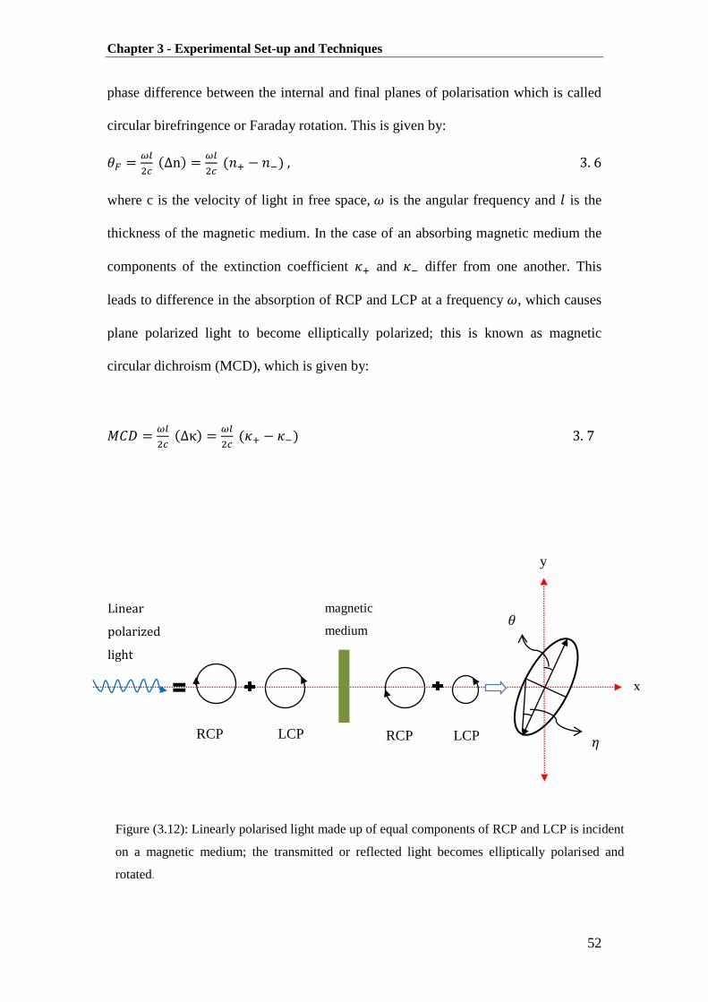
Chapter 3 - Experimental Set-up and Techniques
52
phase difference between the internal and final planes of polarisation which is called
circular birefringence or Faraday rotation. This is given by:
, 3. 6
where c is the velocity of light in free space, is the angular frequency and is the
thickness of the magnetic medium. In the case of an absorbing magnetic medium the
components of the extinction coefficient and differ from one another. This
leads to difference in the absorption of RCP and LCP at a frequency , which causes
plane polarized light to become elliptically polarized; this is known as magnetic
circular dichroism (MCD), which is given by:
3. 7
RCP LCP RCP LCP
magnetic
medium
y
x
Linear
polarized
light
𝜃
𝜂
Figure (3.12): Linearly polarised light made up of equal components of RCP and LCP is incident
on a magnetic medium; the transmitted or reflected light becomes elliptically polarised and
rotated.

Chapter 3 - Experimental Set-up and Techniques
53
Opaque samples are usually studied by reflection where the plane of
polarisation of the light is rotated as it reflected from a magnetised sample; this
phenomenon is known as the Kerr effect. In measurement where the light is
transmitted through the magnetised sample, the plane of polarisation of the light beam
is rotated; this phenomenon is called the Faraday effect.
3.8 Magneto-Optics Set-up and Principles of the Technique
The set-up for measuring the magneto-optical effects is based upon the
Katsuaki Sato method [38]. This technique allows the simultaneous measurement of
the magnetic circular dichroism (MCD) and rotation (θ) of the sample. In addition,
this technique can give a high sensitivity of 0.002º at 500 nm and resolution of 12 nm.
Fig. 3.13 shows a schematic diagram of the magneto-optics set-up which can
be altered between Kerr and Faraday geometry. The Kerr geometry is the most
appropriate geometry to be used when the sample is highly absorbing and effectively
opaque, whereas the Faraday geometry is used when the sample is transparent.
In this set-up either a tungsten or xenon lamp with powers of 150 Watt and
250 Watt were used to cover a wide range of spectra of 0.6-3.8 eV and 1.5- 4.5 eV
respectively. The light from the appropriate source is then aligned to pass through a
Spectro-275 spectrometer in order to give monochromatic light. The required
wavelength can be obtained by selecting between three different diffraction gratings
blazed at different wavelengths. In order to remove the unwanted wavelengths, the
light was filtered using a band-pass filter. The light was then passed through a Glan-
Taylor UV prism polariser to yield the required plane polarised light to pass through
the sample.

Chapter 3 - Experimental Set-up and Techniques
54
Removed by the
author for copyright reasons
Figure 3.13: Schematic diagram of magneto-optics setup in either Faraday or Kerr geometry.
Adapted from ref. [36].
The sample was mounted either on a room temperature sample holder or on
cold-finger cryostat with optical-window/aperture. The sample is then placed
vertically between the poles of an electromagnet which provides a magnetic field of
1.8 T and 0.5 T for room temperature and low temperature measurement respectively.
This difference in the value of the field is due to the fact that the magnet pole-piece
separation had to be increased for low temperature measurement in order to

Chapter 3 - Experimental Set-up and Techniques
55
accommodate the cryostat tail-piece. At low temperature measurement, the cryostat is
evacuated for about 30 minutes before introducing liquid helium to cool the sample
down. An Oxford ITC03
temperature controller was used to set specific temperatures
and measurements could be made over the range from 5 to 400 K. The polarised light
is then focused and aligned to a similar size of aperture, then reflected or transmitted
through the sample onto the photoelastic modulator (PEM). A series of mirrors and
lenses is manoeuvred and used to achieve the optimal alignment so as to keep the
maximum amount of the light passing through the sample and reduce the scattering
within the pole-pieces, which affect the sensitivity of the experiment.
The PEM produces a signal which is proportional to the ellipticity and rotation
of the light. The PEM is a piezo-birefringent modulator which consists of a
birefringent crystal mounted on a piezo-vibrator with modulating frequency, f. The
birefringent crystal vibration causes advancement and retardation in the phase of the
traversing light parallel to the vibration direction [39]. The direction of the
birefringent crystal vibration is set at 45º to the polariser and the modulation of the
retardation is set to a quarter of the light wavelength. This means that the light
emerging from the PEM alternates between RCP and LCP with frequency, f. The
sample will then introduce oscillations, with a frequency f or 2f, in the light intensity,
if it exhibits any MCD, or rotation, whereas the light intensity will remain constant if
the sample shows no magneto-optics effect.
The light is then passed through an analyser and focused onto the
photomultiplier (PMT). This detector converts the light intensity to an electrical signal
then feeds it to a conditioning unit to amplify the signal and split it into an AC and a
DC component. The DC component is recorded using a Keithley voltmeter which can
be controlled via the gain of the PMT. This component has to be constant in order to

Chapter 3 - Experimental Set-up and Techniques
56
maintain a constant sensitivity. The AC component is recorded using two signal-
recovery lock-in amplifiers. The voltmeter and lock-in amplifiers, one and two, are
used to measure the intensities I0, I1f and I2f respectively.
These three intensities, I0 , I1f and I2f , have been calculated by Sato [38] and
are given in the following equations:
[ ] 3.8
3.9
] 3.10
3.11
, 3.12
where I0 represents the intensity constant and J0, J1 and J2 are the Bessel
functions which are proportional to the intensity of light used to determine the
maximum sensitivity of the magneto-optics measurement. The terms t+ and t- are the
Fresnel coefficients for RCP and LCP transmitted light respectively. The symbol δ0 is
the amplitude of the retardation, f the modulation frequency, φ the analyser angle and
Δθ the difference between RCP and LCP.
The Faraday rotation θF and Faraday ellipticity ηF (MCD) can be deduced by
measuring the intensities I0, I1f and I2f as in the Sato’s formulae:
3.13
3.14
Therefore, the values of Δθ and ΔT/T can be calculated from the experimental
values of I2 (f)/ I1 (0) and I3 (2f)/ I1 (0), setting =0, as shown in the following:

Chapter 3 - Experimental Set-up and Techniques
57
3.15
3.16
In order to reduce the noise levels in the magneto-optics data the
measurements are repeated automatically via the controlling PC which runs Labview
software. On the other hand, the data can be calibrated in order to convert them into
real units (degrees). This calibration is achieved by rotating the polariser angle so as
to give a minimum output of I3(2f), then we rotate the analyser over a few degrees
through steps of 1º. The calibration factor is then determined by recording the
resulting change in I3(2f)/I0(0) value at each analyser angle.
3.9 Optical Transmission and Reflection Techniques
The spectra of transmission and reflection were measured directly in order to
determine the absorption spectroscopy. Fig. 3.14 shows the schematic diagram for the
absorption spectroscopy system. In this system the data were recorded at room
temperature using a tungsten halogen lamp with a power of 250 watts to enable us to
cover a wide spectral range from 1.7 eV to 4.5 eV. The set-up can be switched alter
between transmission and reflection geometry via changing the position of the PMT.
The light produced from the lamp is passed through a Specro-275
spectrometer in order to produce monochromatic light. This light is then filtered and
split in two beams: reference and sample beams. These two beams are passed through
an optical chopper with a frequency of 370 MHZ and 310 MHZ respectively. After
leaving the optical chopper, the reference beam is recorded by the PMT, whereas the
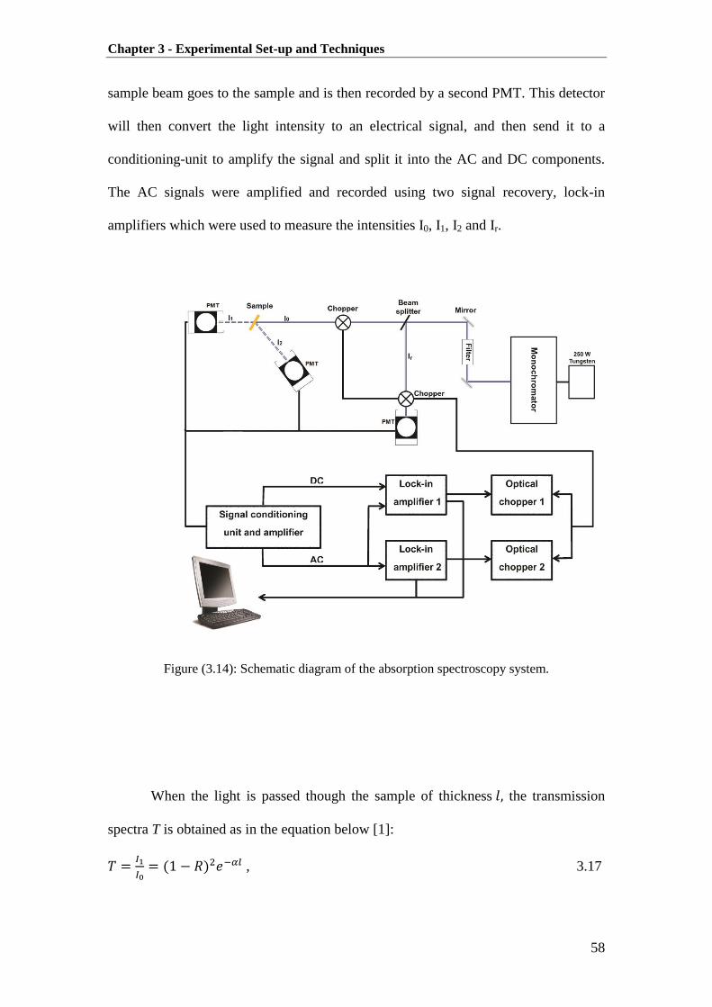
Chapter 3 - Experimental Set-up and Techniques
58
sample beam goes to the sample and is then recorded by a second PMT. This detector
will then convert the light intensity to an electrical signal, and then send it to a
conditioning-unit to amplify the signal and split it into the AC and DC components.
The AC signals were amplified and recorded using two signal recovery, lock-in
amplifiers which were used to measure the intensities I0, I1, I2 and Ir.
Figure (3.14): Schematic diagram of the absorption spectroscopy system.
When the light is passed though the sample of thickness the transmission
spectra T is obtained as in the equation below [1]:
, 3.17
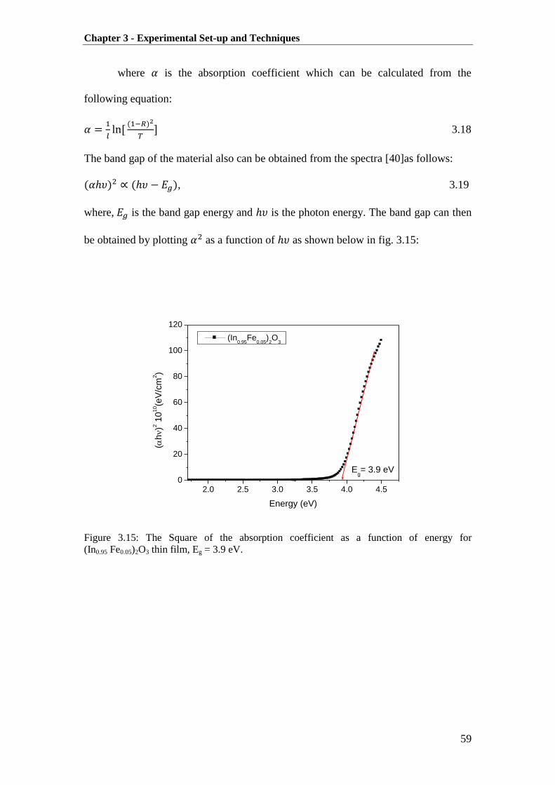
Chapter 3 - Experimental Set-up and Techniques
59
where is the absorption coefficient which can be calculated from the
following equation:
[
] 3.18
The band gap of the material also can be obtained from the spectra [40]as follows:
, 3.19
where, is the band gap energy and is the photon energy. The band gap can then
be obtained by plotting as a function of as shown below in fig. 3.15:
Figure 3.15: The Square of the absorption coefficient as a function of energy for
(In0.95 Fe0.05)2O3 thin film, Eg = 3.9 eV.
2.0 2.5 3.0 3.5 4.0 4.50
20
40
60
80
100
120
Eg= 3.9 eV
(h)2
10
10(e
V/c
m2)
Energy (eV)
(In0.95
Fe0.05
)2O
3

Chapter 3 - Experimental Set-up and Techniques
60
3.10 Thin Films Samples Investigated
In this thesis thin films were prepared in different research groups using different
growth methods. The details of the thin films that were prepared and investigated
during this thesis are illustrated in the table (3.1) below:
Table (3.1): Summary of the content and growth conditions of the samples that were
investigated in this thesis.
Sam
ple
nam
e
Content
Th
ickn
ess
(nm
)
O2 P
ress
ure
(mT
orr
)
Dep
osi
tion
Tem
per
atu
re
( ºC
)
Ann
eali
ng
fo
r
30
min
( º
C )
subst
rate
Dep
osi
tion
met
hod
272Mq
La 0
.7S
r 0.3
MnO
3
81 4×10⁻³
650
No STO
By
PL
D in
S
hef
fiel
d U
niv
ersi
ty
274Mq 74 100
650 No STO
304Mq 130 200 650 No STO
306Mq 87 300 650 No STO
271Mq 100 4×10
-3
650 No Sapphire
273Mq 115 100 650
No Sapphire
301Mq 110
200 650 No Sapphire
303Mq 80
300 650 No Sapphire
260Mq
La 0
.5S
r 0.5
MnO
3
132 4×10⁻³
650 No STO
262Mq 80 100 650 No STO
264Mq 69 200 650
No STO
270Mq 63 300 650 No STO

Chapter 3 - Experimental Set-up and Techniques
61
Sam
ple
nam
e
Content
Th
ickn
ess
(nm
)
O2 P
ress
ure
(mT
orr
)
Dep
osi
tion
Tem
per
atu
re
( ºC
)
Ann
eali
ng
fo
r
30
min
( º
C )
subst
rate
Dep
osi
tion
met
hod
259Mq L
a 0.5
Sr 0
.5M
nO
3
105 4×10⁻³
650
No Sapphire
By
PL
D in
S
hef
fiel
d U
niv
ersi
ty
261Mq 75 100
650 No Sapphire
263Mq 50 200 650 No Sapphire
269Mq 105 300 650 No Sapphire
321Mq
La 0
.85S
r 0.1
5M
nO
3
82 4×10⁻³
650 No STO
323Mq 59 100 650 No STO
324Mq 91 200 650
No STO
325Mq 100 300 650 No STO
320Mq 100 5×10⁻³
650 No Sapphire
322Mq 90 100 650 No Sapphire
326Mq 89 200 650 No Sapphire
327Mq 92 300 650 No Sapphire
520Mq La0.7Sr0.3MnO3 50 300 650 No STO
521Mq La0.7Sr0.3MnO3 200 300 650 No STO
Yam001 GdMnO3 100 1-2 650 No STO
By
Sp
utt
erin
g
in
Mosc
ow
Yam002 GdMnO3 100 1-2 650 No LAO
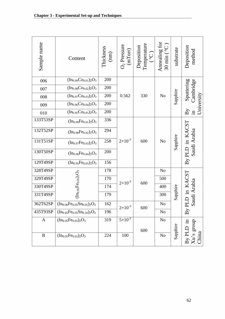
Chapter 3 - Experimental Set-up and Techniques
62
Sam
ple
nam
e
Content
Th
ickn
ess
(nm
)
O2 P
ress
ure
(mT
orr
)
Dep
osi
tion
Tem
per
atu
re
( ºC
)
Ann
eali
ng
fo
r
30
min
( º
C )
subst
rate
Dep
osi
tion
met
hod
006 (In0.99Co0.01)2O3 200
0.562 330 No
Sap
phir
e
By
S
pu
tter
ing
in
Cam
bri
dg
e
Univ
ersi
ty
007 (In0.98Co0.02)2O3 200
008 (In0.97Co0.03)2O3 200
009 (In0.96Co0.04)2O3 200
010 (In0.95Co0.05)2O3 200
133T53SP (In0.99Fe0.01)2O3 336
2×10⁻³
600 No
Sap
phir
e
By
PL
D in
K
AC
ST
Sau
di
Ara
bia
132T52SP (In0.98Fe0.02)2O3 294
131T51SP (In0.97Fe0.03)2O3 258
130T50SP (In0.96Fe0.04)2O3 200
129T49SP (In0.95Fe0.05)2O3 156
328T49SP
(In
0.9
5F
e 0.0
5) 2
O3 178
2×10⁻³ 600
No S
apphir
e
By
PL
D in
K
AC
ST
Sau
di
Ara
bia
329T49SP 170 500
330T49SP 174 400
331T49SP 179 300
362T62SP (In0.90Fe0.05Sn0.05)2O3 162 2×10
-3 600 No
435T93SP (In0.85Fe0.05Sn0.10)2O3 196 No
A (In0.95Fe0.05)2O3 319 5×10⁻²
600
No
Sap
phir
e
By
PL
D in
Xu’s
gro
up
Ch
ina
B (In0.95Fe0.05)2O3 224 100 No

Chapter 3 - Experimental Set-up and Techniques
63
3.11 References
1. M. Fox, Optical properties of solids. (Oxford University Press, Oxford ; New
York, 2001).
2. N. A. Spaldin, Magnetic materials : fundamentals and device applications.
(Cambridge University Press, Cambridge, Uk ; New York, 2003).
3. W. Prellier, L. Ph and B. Mercey, Journal of Physics: Condensed Matter 13
(48), R915 (2001).
4. L. M. Wang, H. H. Sung, B. T. Su, H. C. Yang and H. E. Horng, Journal of
Applied Physics 88 (7), 4236-4240 (2000).
5. G. J. Snyder, R. Hiskes, S. DiCarolis, M. R. Beasley and T. H. Geballe,
Physical Review B 53 (21), 14434-14444 (1996).
6. R. von Helmolt, J. Wecker, B. Holzapfel, L. Schultz and K. Samwer, Physical
Review Letters 71 (14), 2331-2333 (1993).
7. O. Akira and T. Atsushi, Semiconductor Science and Technology 20 (4), S1
(2005).
8. J. Wilson and J. F. B. Hawkes, Lasers, principles and applications. (Prentice
Hall, New York, 1987).
9. O. Svelto and D. C. Hanna, Principles of lasers, 3rd ed. (Plenum, New York,
1989).
10. L. I. Grossweiner, L. R. Jones, J. B. Grossweiner and B. H. G. Rogers, The
science of phototherapy : an introduction. (Springer, Dordrecht ; Norwell,
MA, 2005).
11. C. B. Hitz, J. J. Ewing and J. Hecht, Introduction to laser technology, 3rd ed.
(IEEE Press, New York, 2001).
Chapter 3 - Experimental Set-up and Techniques
64
12. D. B. Chrisey and G. K. Hubler, Pulsed laser deposition of thin films. (J.
Wiley, New York, 1994).
13. W. Prellier, A. M. Haghiri-Gosnet, B. Mercey, P. Lecoeur, M. Hervieu, C.
Simon and B. Raveau, Applied Physics Letters 77 (7), 1023-1025 (2000).
14. M. Ziese, S. P. Sena and H. J. Blythe, Journal of Magnetism and Magnetic
Materials 202 (2–3), 292-300 (1999).
15. D. A. Eastham, Atomic physics of lasers. (Taylor & Francis, London ;
Philadelphia, 1986).
16. D. Basting and G. Marowsky, Excimer laser technology. (Springer/Praxis,
Berlin ; New York, 2005).
17. X. Y. Chen, S. B. Xiong, Z. S. Sha and Z. G. Liu, Applied Surface Science
115 (3), 279-284 (1997).
18. D. J. Lichtenwalner, O. Auciello, R. Dat and A. I. Kingon, Journal of Applied
Physics 74 (12), 7497-7505 (1993).
19. G. Koster, B. L. Kropman, G. J. H. M. Rijnders, D. H. A. Blank and H.
Rogalla, Applied Physics Letters 73 (20), 2920-2922 (1998).
20. M. Lippmaa, N. Nakagawa, M. Kawasaki, S. Ohashi and H. Koinuma,
Applied Physics Letters 76 (17), 2439-2441 (2000).
21. T. Ohnishi, K. Shibuya, T. Yamamoto and M. Lippmaa, Journal of Applied
Physics 103 (10), 103703-103706 (2008).
22. A. Ohtomo and H. Y. Hwang, Journal of Applied Physics 102 (8), 083704-
083706 (2007).
23. J. F. Lawler, J. M. D. Coey, J. G. Lunney and V. Skumryev, Journal of
Physics: Condensed Matter 8 (49), 10737 (1996).

Chapter 3 - Experimental Set-up and Techniques
65
24. H. Nguyen Hoa, S. Joe and H. Awatef, Journal of Physics: Condensed Matter
17 (1), 199 (2005).
25. L. S. Dorneles, D. O’Mahony, C. B. Fitzgerald, F. McGee, M. Venkatesan, I.
Stanca, J. G. Lunney and J. M. D. Coey, Applied Surface Science 248 (1–4),
406-410 (2005).
26. E. van de Riet, J. C. S. Kools and J. Dieleman, Journal of Applied Physics 73
(12), 8290-8296 (1993).
27. A. J. Behan, A. Mokhtari, H. J. Blythe, M. Ziese, A. M. Fox and G. A.
Gehring, Journal of Physics: Condensed Matter 21 (34), 346001 (2009).
28. Z. L. Wang and A. J. Shapiro, Surface Science 328 (1–2), 141-158 (1995).
29. M. Ziese, H. C. Semmelhack, K. H. Han, S. P. Sena and H. J. Blythe, Journal
of Applied Physics 91 (12), 9930-9936 (2002).
30. R. L. Fagaly, Review of Scientific Instruments 77 (10), 101101-101145
(2006).
31. M. P. Janawadkar, R. Baskaran, R. Saha, K. Gireesan, R. Nagendran, L. S.
Vaidhyanathan, J. Jayapandian and T. S. Radhakrishnan, Current Science 77
(6), 759-769 (1999).
32. J. Clarke, Proceedings of the IEEE 77 (8), 1208-1223 (1989).
33. Y. Zhuravlev and D. Rassi, Squids and their applications. (World Scientific
Publ Co Pte Ltd, Singapore, 2000).
34. H. Prance, T. D. Clark, R. Whiteman, R. J. Prance, M. Everitt, P. Stiffell and
J. F. Ralph, Physical Review E 64 (1), 016208 (2001).
35. Josephso.Bd, Science 184 (4136), 527-530 (1974).
36. A. Behan, Sheffield university, 2008.
37. S.P.Sena, Sheffield University, 1998.

Chapter 3 - Experimental Set-up and Techniques
66
38. K. Sato, Japanese Journal of Applied Physics 20 (12), 2403-2409 (1981).
39. K. W. Hipps and G. A. Crosby, The Journal of Physical Chemistry 83 (5),
555-562 (1979).
40. N. G. Patel and B. H. Lashkari, Journal of Materials Science 27 (11), 3026-
3031 (1992).

Chapter 4 - Lanthanum Strontium Manganite (LSMO)
67
Chapter 4
Lanthanum Strontium Manganite (LSMO)
4.1 Introduction
In the last decades, mixed-valence perovskite manganites have been shown to
have very exciting characteristics from both a basic research and a technological
viewpoint. This is due to the discovery of the phenomenon of colossal
magnetoresistance (CMR) in thin manganite films. CMR is the very large change in
resistance produced by the application of an external magnetic field [1].
The general chemical formula of the perovskites is where T is
a trivalent rare earth cation ( T = La, Pr, Nd….....) and is a divalent alkaline-earth
cation (D = Ca, Sr, Ba……). Amongst a wide range of perovskite-type of manganites
with different combinations of T and, D, ( ) (LSMO) is considered to
be an ideal reference material [2-7]. The compound is found to be an
antiferromagnetic insulator with a Néel temperature ( ) of about 140 K. Below its
Curie temperature (TC) the ferromagnetic state in is found to be dependent
upon oxygen stoichiometry and the doping level of Sr ions [4]. The maximum value
of has been found to be 380 K for the bulk crystals at a doping level of
[8]. Magneto-optics and optical properties of thin films provide useful information
about the spin-dependent electronic structure which is very useful to determine the
nature of the ferromagnetism. The intention is that these films could be used as
magnetic devices such as magnetic field sensors [4, 9-10].

Chapter 4 - Lanthanum Strontium Manganite (LSMO)
68
This chapter investigates the magnetic properties of LSMO thin films
deposited under various growth conditions. Magneto-optical properties were
investigated in order to provide information about the polarisation of mobile electrons
below the of the LSMO films.
4.2 Literature Review on LSMO
The ideal perovskite structure consists of six oxygen atoms arranged around
each Mn atom to form an octahedron as indicated in fig 4.1.
Figure (4.1): Sketch of the cubic perovskite unit-cell for manganites.
There are a large number of cations that can occupy the A and B sites in
the cubic perovskite structure, which may be set at body-center or cube corner.
The A sites of this structure are occupied by a trivalent or divalent ion, which
leads to mixed valency of the transition metal ions ⁄ which occupy B sites
[2, 11-13]. In this thesis we consider compounds where the B sites are always
A site (La, Sr, Ca, ….)
B site (Mn)
Oxygen (O)

Chapter 4 - Lanthanum Strontium Manganite (LSMO)
69
occupied by Mn atoms. The mixed-valence oxides can be regarded as solid solutions
between end members and with formal valence states
and
, leading to mixed-valence compounds such as
(
)(
) . The electronic configurations of and are
and , respectively [14].
The crystal structure of ( ) was studied towards the end of the
1940s by Janker and Van Santen [12, 14]. It was found that the ferromagnetism is
related to the simultaneous existence of and ions and [15-16] appears in
the range of . Both of the end members are antiferromagnetic and
insulating, whereas when the solid-solutions are both ferromagnetic and
conducting. The system at exhibits a very interesting
state because it becomes ferromagnetic and exhibits a metal-insulator transition at
[14, 17]. The expected magnetisation (M) from the LSMO per Mn ion can be
calculated as following:
M= [ ( ) ( )]
= ( ) , (1)
where , is the doping level and the Bohr magneton
The main effects of the various substitutions are to vary the strain and the
number of electrons in the 3d band, where the mixed valency leads to a strong
ferromagnetic interaction (FM). Verwey and de Boer discovered that the mixed
valence can lead to metallic conduction [2, 14]. The phase diagram of the perovskite
manganites is very complex, as is shown in fig. 4.2 for ( ) [18].
There are now hundreds of papers focused on the phase diagrams of the manganites
[18-22]

Chapter 4 - Lanthanum Strontium Manganite (LSMO)
70
Removed by the
author for copyright reasons
Figure (4.2): phase diagram of ( ) as a function of temperature and doping
level . PI - paramagnetic insulator; PM - paramagnetic metal; CI- spin canted insulator; FI-
ferromagnetic insulator; FM- ferromagnetic metal; AFM- antiferromagnetic metal ; - Curie
temperature; - Neel temperature [18].
Theoretically, the manganite system is usually described by the 3d orbitals of
the Mn in a cubic lattice, because the other orbitals are some distance from the Fermi
level. The crystal field splits the 3d orbitals into two higher energy levels and three
lower energy levels. The states are occupied by three electrons with parallel
spin. There is only one electron in one of the two states for . This electron
has its spin parallel to the three electrons in the levels due to Hund’s rule [15]. It
has been found that the width of the band is approximately and the separation
between and is about [15, 23]. Several studies predict that the band
structure of ( ) is very close to be half-metallic system. However,
spin polarization of conduction electron is still not proven [10]. Hence the half-
metal has an energy gap in one spin and metal with Fermi surface for the opposite

Chapter 4 - Lanthanum Strontium Manganite (LSMO)
71
spins. In the optimally doped manganite ( ) the up-spins are
localized and the down-spins are delocalized or vice versa. As far as conduction is
concerned, only one spin contributes to the conduction. In the particular example
shown in fig. 4.3 spin-up electrons can travel through the system, and the LSMO
behaves as a half-metal. In this case the magnetic moment should be 3.7 . However
the measurement values did not exceed 3.6 and there is evidence from band
calculations for some minority spin electrons at the bottom of the spin-down band due
to occupation of the Mn t2g spin states. Hence the spin-up Mn(eg) are the mobile
electrons and the spin-down Mn(t2g) are immobile electrons, as shown in the
schematic band structure fig. 4.3 [24-25].
Removed by the
author for copyright reasons
Figure (4.3): Schematic representation of the electronic band structure of half-metallic
( ) [24].
Chapter 4 - Lanthanum Strontium Manganite (LSMO)
72
Double exchange (DE) is the first theory that explains the mechanism of both
ferromagnetism and antiferromagnetism. It can be considered as a system of two
cations separated by an anion. The DE mechanism describes the localized
electrons as classical spins of value
and coupled to the mobile electrons
according to Hund's rules. The requirement to optimise the kinetic energy of the
mobile electrons favours a spin polarised ground state [2, 11, 26-27]. In the case of
the undoped manganite material ( ) ( ) only (3d4) ions are
present. The Jahn-Teller effect splits the eg band making LaMnO3 an
antiferromagnetic insulator. Doping with a small amount of ions lead to an
increase in the , introduced holes into the eg band, because the ion is
replaced by the ion Therefore, exchanges the extra electron with
and this exchange occurs via 2p orbitals of the ions. According to Hund’s
coupling, this only will become possible if the spins of eg electrons are parallel to the
core spin of the t2g electrons. The DE mechanism occurs by transfer of a p electron
from the ion to the ion. This is accompanied by transfer of an electron
from the to the O ion, replacing the previous one, as indicated in fig. 4.4.
Hund’s rule requires that, for the lowest energy, the electron in the shell
should always be spin-aligned, because of the large Hund’s rule coupling. However,
the strain influences spin-ordering and orbital-ordering in manganite via an elongation
or compression of the oxygen octahedron (MnO6). This leads to a Jahn-Teller
distortion which splits the degeneracies of the eg and t2g levels [28].
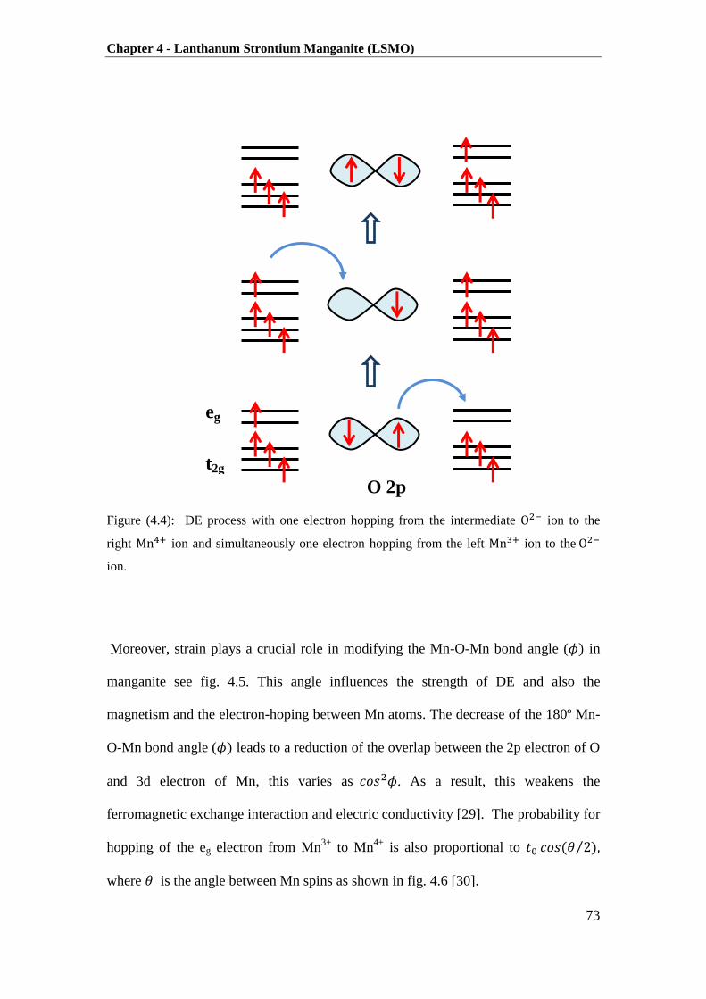
Chapter 4 - Lanthanum Strontium Manganite (LSMO)
73
Figure (4.4): DE process with one electron hopping from the intermediate ion to the
right ion and simultaneously one electron hopping from the left ion to the
ion.
Moreover, strain plays a crucial role in modifying the Mn-O-Mn bond angle ( ) in
manganite see fig. 4.5. This angle influences the strength of DE and also the
magnetism and the electron-hoping between Mn atoms. The decrease of the 180º Mn-
O-Mn bond angle ( ) leads to a reduction of the overlap between the 2p electron of O
and 3d electron of Mn, this varies as . As a result, this weakens the
ferromagnetic exchange interaction and electric conductivity [29]. The probability for
hopping of the eg electron from Mn3+
to Mn4+
is also proportional to ( ⁄ )
where is the angle between Mn spins as shown in fig. 4.6 [30].
O 2p
t2g
eg
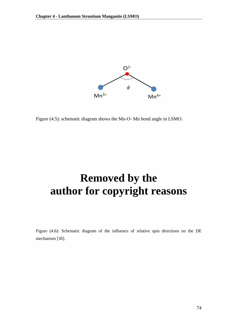
Chapter 4 - Lanthanum Strontium Manganite (LSMO)
74
Figure (4.5): schematic diagram shows the Mn-O- Mn bond angle in LSMO.
Removed by the
author for copyright reasons
Figure (4.6): Schematic diagram of the influence of relative spin directions on the DE
mechanism [30].

Chapter 4 - Lanthanum Strontium Manganite (LSMO)
75
Among the various ( ) compositions many of research
groups have focused on thin films of composition ( ) , which
exhibit high TC. The TC and metal-insulator transition TMI are required to be above
room temperature in spintronics application. However, TMI is found to be very close
to TC for bulk single crystals and epitaxial films, whereas TMI is much lower in
polycrystalline LSMO. This difference is related to the structural defects which
depend on the growth conditions [6, 31-33]. The highest TC is found to be about
380 K for the bulk crystals of ( ) whereas TC is reduced in the case
of thin films of this composition [8].
Magnetic properties and Tc are found to be very sensitive to the particular
growth conditions such as: method of fabrication, substrate material, growth
temperature, annealing temperature and film thickness [31, 34]. Many studies
reported that the observed differences in magnetic properties are related to strain
which, in turn, depends on the lattice mismatch between the film and the substrate [8,
35-37]. The effects of strain on the physical properties of the manganites are, at the
present time, not fully understood. However, the strain is not only the factor that
affects the film’s properties.
Epitaxial LSMO films have been grown using PLD on different substrates
with different orientations [31, 38-41]. It has been found that substrates play an
important role for the magnetic and transport properties of the films [42].The most
common substrates that have been used to grow epitaxial LSMO films are strontium
titanate, SrTiO3 (STO), and lanthanum aluminate, LaAlO3 (LAO), [43]. The c-axis
lattice constant of the LSMO film is about 0.389 nm and the lattice constants for STO
and LAO substrates are about 0.391 nm and 0.379 nm, respectively [35]. The LSMO
films grown on STO substrates exhibit an in-plane easy magnetisation direction

Chapter 4 - Lanthanum Strontium Manganite (LSMO)
76
whereas the films exhibit an out-of plan easy direction, on LAO substrates [35]. In
addition, a LSMO thin film has been grown on a sapphire substrate using the PLD
technique. However, the sapphire substrate and LSMO are completely different in
symmetries and lattice spacings [43].
H.Y.Hwang et al have reported that the resistivity ( ) for single crystal and
polycrystalline ( ⁄ ⁄ ) show a sharp drop at TC= 365 K. Despite the
temperature dependence of the magnetization, TC measured in is very similar in
single-crystal and poly-crystalline as indicated in fig. 4.7 [44].
Removed by the
author for copyright reasons
Figure (4.7) Top panel: ( )of ( ⁄ ⁄ ) for a single-crystal sample and two
polycrystalline samples with final sintering temperatures of 1300 and 1700 . Bottom
panel: the temperature dependence magnetisation for three samples at 0.5 T. Inset: The field
dependent magnetisation of these samples at 5 and 280 K [44].

Chapter 4 - Lanthanum Strontium Manganite (LSMO)
77
It is clear that the resistivity ( ) depends on the sample quality, whereas the
magnetisation is far less dependent. Hence the magnetisation is dominated by grain
volumes whereas the resistivity is dominated by the intermediate area between the
grains which act as an insulating and spin-scattering zone when the electrons hop
from one magnetic domain to another [31, 45].
Thin films of ( ) grown on STO substrates showing
superior magnetic and electrical properties have been reported [9] where the
magnetisation ( ), and TC were 170 ⁄ and , respectively. The metal-
insulator transition temperature, TMI was 360K, coinciding with TC.
A.K.Pradhan et al reported that for ( ) deposited on STO the
TC was close to that for bulk material. However, TC decreases sharply with decreasing
film thickness below a critical thickness of about 55 nm [13] as illustrated in fig. 4.8.
This unusually large thickness dependence could be attributed to the strain or to a
dead layer.
Removed by the
author for copyright reasons
Figure (4.8): The temperature dependence of magnetization of LSMO/STO films of varying
thickness. The inset shows the enlarged graphs for 22 nm and 12 nm thick films [13].
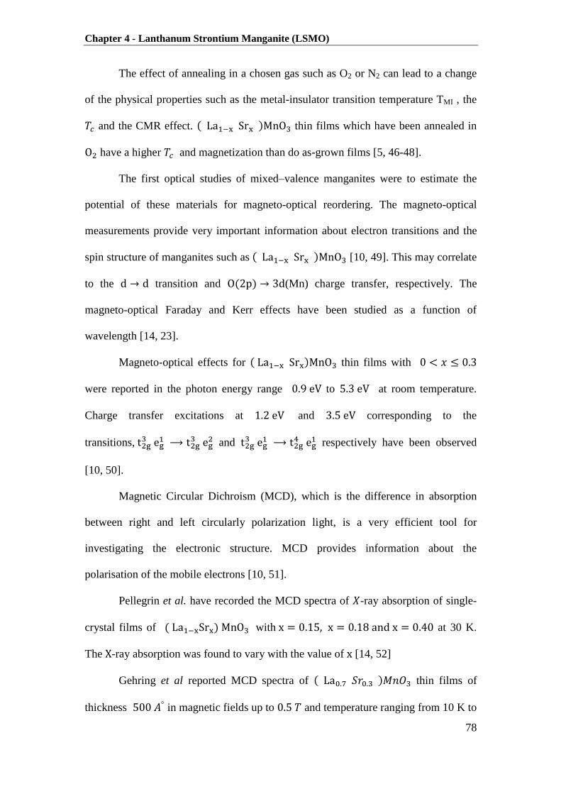
Chapter 4 - Lanthanum Strontium Manganite (LSMO)
78
The effect of annealing in a chosen gas such as O2 or N2 can lead to a change
of the physical properties such as the metal-insulator transition temperature TMI , the
and the CMR effect. ( ) thin films which have been annealed in
have a higher and magnetization than do as-grown films [5, 46-48].
The first optical studies of mixed–valence manganites were to estimate the
potential of these materials for magneto-optical reordering. The magneto-optical
measurements provide very important information about electron transitions and the
spin structure of manganites such as ( ) [10, 49]. This may correlate
to the transition and ( ) (Mn) charge transfer, respectively. The
magneto-optical Faraday and Kerr effects have been studied as a function of
wavelength [14, 23].
Magneto-optical effects for ( ) thin films with
were reported in the photon energy range to at room temperature.
Charge transfer excitations at and corresponding to the
transitions,
and
respectively have been observed
[10, 50].
Magnetic Circular Dichroism (MCD), which is the difference in absorption
between right and left circularly polarization light, is a very efficient tool for
investigating the electronic structure. MCD provides information about the
polarisation of the mobile electrons [10, 51].
Pellegrin et al. have recorded the MCD spectra of -ray absorption of single-
crystal films of ( ) with at 30 K.
The -ray absorption was found to vary with the value of [14, 52]
Gehring et al reported MCD spectra of ( ) thin films of
thickness in magnetic fields up to and temperature ranging from 10 K to

Chapter 4 - Lanthanum Strontium Manganite (LSMO)
79
450 K. It was found that the spectra peak at about and the peak position moved
toward lower energy when the temperature is increased, as indicated in fig. 4.9 [10].
Removed by the
author for copyright reasons
Figure (4.9): MCD measurements of epitaxial LSMO films grown on (001) La0.3Sr0.7
Al0.65Ta0.35O9 (LSAT) substrates at T= 10, 55, 100, 150, 200, 250, 300, 350 and 400 K with a
magnet field of 0.5 T applied along the [001] direction of the film [10] .
4.3 Experiment Results and Discussion
In order to investigate the magnetic and magneto-optical properties of LSMO,
two groups of ( ) films with = 0.15, 0.3 and 0.5 were deposited
onto STO (001) and sapphire (0001) substrates. The LSMO target was prepared from
high purity La2O3, SrCO3 and MnO2 powders. The stoichiometric mixture were
heated and re-ground in air at 800, 1000 and 1200 for 16 hours. The result is
LSMO calcined powder that was then pressed at 25,000 Pa and sintered at 1400 for
12 hours in order to give a high density target. The film growth was carried out by
PLD. The films were grown at a deposition temperature of 650 in an oxygen

Chapter 4 - Lanthanum Strontium Manganite (LSMO)
80
partial pressure ranging from 4 ×10⁻³
mTorr to 300 mTorr. Fig. 4.10 shows the XRD
patterns of the LSMO film grown on an STO substrate at base pressure (4×10⁻³
mTorr) and at 300 mTorr. These data were measured by Ali Hakimi in the laboratory
of Cambridge University. XRD patterns indicate a number of secondary phases in the
film grown at base pressure. The film grown in a higher oxygen pressure (300 mTorr)
is single-phase (red line), is oriented with the STO substrate and we see reflection
peaks which correspond to LSMO (002), (004), (006). Many STO substrate peaks are
present; these peaks are obviously very sharp.
Figure (4.10): The XRD pattern of ( ) films grown on STO at base
pressure and 300 mTorr. The X-ray wavelength was 1.5406 .
10 20 30 40 50 60 70 80 90 100
4
6
8
10
12
14
16
Mn
3O
4 (
400
)
006
004
002
Ln
in
ten
sity (
arb
.un
its)
2 (degree)
4× 10⁻³ mTorr
300 mTorr
LSMO/STO
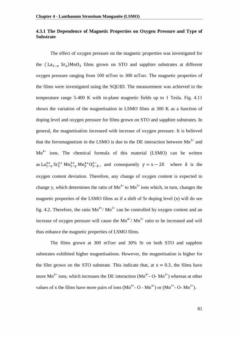
Chapter 4 - Lanthanum Strontium Manganite (LSMO)
81
4.3.1 The Dependence of Magnetic Properties on Oxygen Pressure and Type of
Substrate
The effect of oxygen pressure on the magnetic properties was investigated for
the ( ) films grown on STO and sapphire substrates at different
oxygen pressure ranging from 100 mTorr to 300 mTorr. The magnetic properties of
the films were investigated using the SQUID. The measurement was achieved in the
temperature range 5-400 K with in-plane magnetic fields up to 1 Tesla. Fig. 4.11
shows the variation of the magnetisation in LSMO films at 300 K as a function of
doping level and oxygen pressure for films grown on STO and sapphire substrates. In
general, the magnetisation increased with increase of oxygen pressure. It is believed
that the ferromagnetism in the LSMO is due to the DE interaction between Mn3+
and
Mn4+
ions. The chemical formula of this material (LSMO) can be written
as
, and consequently where is the
oxygen content deviation. Therefore, any change of oxygen content is expected to
change y, which determines the ratio of Mn4+
to Mn3+
ions which, in turn, changes the
magnetic properties of the LSMO films as if a shift of Sr doping level ( ) will do see
fig. 4.2. Therefore, the ratio Mn4+
/ Mn3+
can be controlled by oxygen content and an
increase of oxygen pressure will cause the Mn4+
/ Mn3+
ratio to be increased and will
thus enhance the magnetic properties of LSMO films.
The films grown at 300 mTorr and 30% Sr on both STO and sapphire
substrates exhibited higher magnetisations. However, the magnetisation is higher for
the film grown on the STO substrate. This indicate that, at , the films have
more Mn4+
ions, which increases the DE interaction (Mn4+
- O- Mn3+
) whereas at other
values of the films have more pairs of ions (Mn4+
- O - Mn4+
) or (Mn3+
- O- Mn3+
).

Chapter 4 - Lanthanum Strontium Manganite (LSMO)
82
Subsequently, the LSMO films with 30% Sr doping level grown on STO and
sapphire substrates were used for further studies in order to investigate their magnetic
and magneto-optical properties.
Fig. 4.12 shows the TC dependence on Sr doping level for films grown at
300 mTorr and the TC dependence on oxygen pressure for a 30% Sr doping of LSMO
films on STO and sapphire substrates. The temperature dependence of the
magnetisation was measured using the ZFC mode under in-plane field of 0.1 T and
the TC was defined as the temperature corresponding to the minimum of dM/dT. The
highest value of TC was at and increased with increasing oxygen pressure.
The TC value is 340 K for the LSMO film grown at 300 mTorr on both STO and
sapphire substrates. This reveals that the magnetic properties of LSMO films are
strongly affected by oxygen pressure during the growth, as well as by the doping
Figure (4.11): The saturation magnetisation at 300 K as a function of Sr doping level and
oxygen growth pressure of ( ) films grown on a) STO substrate b) Sapphire
substrate.
10 15 20 25 30 35 40 45 50 55
0
20
40
60
80
100
120
140
160
a
LSMO/STO
300K
base pressure
100 mTorr
200 mtorr
300 mTorr
Ma
gn
etisa
tio
n (
em
u/c
m3)
Sr content (%)10 15 20 25 30 35 40 45 50 55
0
20
40
60
80
100
120
140
160
b
LSMO/Sapphire
300K
base pressure
100 mTorr
200 mTorr
300mTorr
Magnetisation(e
mu/c
m3)
Sr content (%)

Chapter 4 - Lanthanum Strontium Manganite (LSMO)
83
level. Moreover, the result displayed very good evidence that the quality of the LSMO
films was improved by increasing oxygen pressure, especially for films grown on the
sapphire substrates.
Fig.4.13 shows ZFC measurement made in-plane in a field of 0.1 T with
variation of oxygen pressure; the ferromagnetic order and TC of these films are
enhanced. A value of 340 K was obtained for both films grown on STO and sapphire
substrates at 300 mTorr with thickness of 87 nm and 80 nm respectively. This LSMO
film exhibits a high value of TC=340 K compared to the previous study for the same
composition, in which a film of 300 nm of LSMO grown on STO gave TC =358 K and
360 K for the film of 100-200 nm thick [13, 53].
Figure (4.12): a) Variation of TC of ( ) films grown on STO and sapphire
substrate at 300 mTorr as a function of Sr doping level. b) Variation of TC of ( )
films grown on STO and sapphire substrate as a function of oxygen pressure.
0.1 0.2 0.3 0.4 0.5
240
260
280
300
320
340
360
a
Curie tem
pera
ture
(T
C)
Sr Content (%)
STO
Sapphire
300mTorr
100 150 200 250 300
180
200
220
240
260
280
300
320
340
360
b
Cu
rie
te
mp
era
ture
(T
C)
Oxygen pressure (mTorr)
STO
Sapphire
x=30%
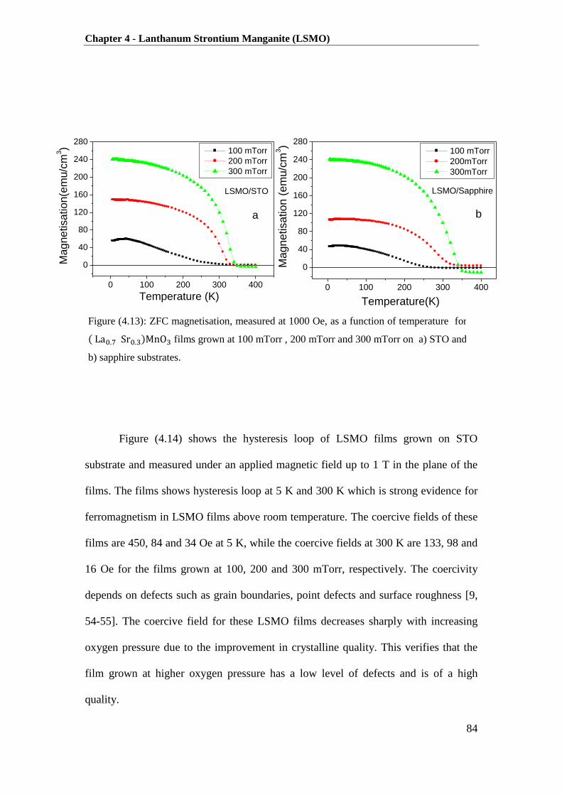
Chapter 4 - Lanthanum Strontium Manganite (LSMO)
84
Figure (4.14) shows the hysteresis loop of LSMO films grown on STO
substrate and measured under an applied magnetic field up to 1 T in the plane of the
films. The films shows hysteresis loop at 5 K and 300 K which is strong evidence for
ferromagnetism in LSMO films above room temperature. The coercive fields of these
films are 450, 84 and 34 Oe at 5 K, while the coercive fields at 300 K are 133, 98 and
16 Oe for the films grown at 100, 200 and 300 mTorr, respectively. The coercivity
depends on defects such as grain boundaries, point defects and surface roughness [9,
54-55]. The coercive field for these LSMO films decreases sharply with increasing
oxygen pressure due to the improvement in crystalline quality. This verifies that the
film grown at higher oxygen pressure has a low level of defects and is of a high
quality.
Figure (4.13): ZFC magnetisation, measured at 1000 Oe, as a function of temperature for
( ) films grown at 100 mTorr , 200 mTorr and 300 mTorr on a) STO and
b) sapphire substrates.
0 100 200 300 400
0
40
80
120
160
200
240
280
a
LSMO/STO
Magnetisation(e
mu/c
m3)
Temperature (K)
100 mTorr
200 mTorr
300 mTorr
0 100 200 300 400
0
40
80
120
160
200
240
280
b
LSMO/Sapphire
Magnetisation (
em
u/c
m3)
Temperature(K)
100 mTorr
200mTorr
300mTorr
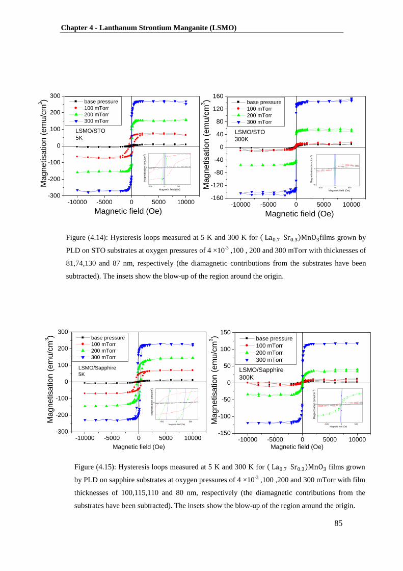
Chapter 4 - Lanthanum Strontium Manganite (LSMO)
85
Figure (4.15): Hysteresis loops measured at 5 K and 300 K for ( ) films grown
by PLD on sapphire substrates at oxygen pressures of 4 ×10⁻³
,100 ,200 and 300 mTorr with film
thicknesses of 100,115,110 and 80 nm, respectively (the diamagnetic contributions from the
substrates have been subtracted). The insets show the blow-up of the region around the origin.
Figure (4.14): Hysteresis loops measured at 5 K and 300 K for ( ) films grown by
PLD on STO substrates at oxygen pressures of 4 ×10⁻³
,100 , 200 and 300 mTorr with thicknesses of
81,74,130 and 87 nm, respectively (the diamagnetic contributions from the substrates have been
subtracted). The insets show the blow-up of the region around the origin.
-10000 -5000 0 5000 10000-300
-200
-100
0
100
200
300
-500 0 500
0
Ma
gnetisation (
em
u/c
m3)
Magnetic field (Oe)
LSMO/Sapphire
5K
base pressure
100 mTorr
200 mTorr
300 mTorr
Magnetisation (
em
u/c
m3)
Magnetic field (Oe)
-10000 -5000 0 5000 10000-150
-100
-50
0
50
100
150
-500 0 500
0
Magnetisation (
em
u/c
m3)
Magnetic field (Oe)
LSMO/Sapphire
300K
base pressure
100 mTorr
200 mTorr
300 mTorr
Ma
gn
etisa
tio
n (
em
u/c
m3)
Magnetic field (Oe)
-10000 -5000 0 5000 10000-300
-200
-100
0
100
200
300
-700 0 700
0
Magne
tisatio
n (
em
u/c
m3)
Magnetic field (Oe)
LSMO/STO
5K
base pressure
100 mTorr
200 mTorr
300 mTorr
Mag
ne
tisation
(e
mu/c
m3)
Magnetic field (Oe)-10000 -5000 0 5000 10000
-160
-120
-80
-40
0
40
80
120
160
-600 0 600
-40
0
Ma
gne
tisa
tion (
em
u/c
m3)
Magnetic field (Oe)
LSMO/STO
300K
base pressure
100 mTorr
200 mTorr
300 mTorr
Ma
gn
etisa
tio
n (
em
u/c
m3)
Magnetic field (Oe)

Chapter 4 - Lanthanum Strontium Manganite (LSMO)
86
The hysteresis loops corresponding to the LSMO films grown on sapphire
substrates (Fig. 4.15) show that the magnetisation behaviour is similar to the LSMO
films grown on STO. The magnetisation increases with increase of oxygen pressure,
whereas the coercive fields of these films decrease with increase of oxygen pressure.
4.3.2 Dependence of Magnetic Properties on Film Thickness
In order to investigate the influence of film thickness on the physical
properties of LSMO thin films, three thin films of ( ) with thicknesses
of 50, 87 and 200 nm were grown on STO (001) substrates by PLD. The films were
deposited under 300 mTorr of oxygen and the substrate temperature was maintained
at 650 K. Fig. 4.16 shows temperature dependence of ZFC measurements with an in-
plane field of 0.1 T. The LSMO films with thickness 50, 87 and 200 nm exhibit TC at
320±16, 340±10 and 350±12 K respectively. The variation of TC with film thickness
may be related to a strain induced lattice mismatch between films and substrates. It
has already been reported that the strain relaxation of lattice mismatch between the
film and the substrate at the interfaces occurs as the film thickness increases [13].
These data show a magnetisation of about140 emu/cm3
for the film with thickness
50 nm as compared with the previous study [13] fig. 4.5, which had a magnetisation at
about 180 emu/cm3 for the film with thickness 55 nm.
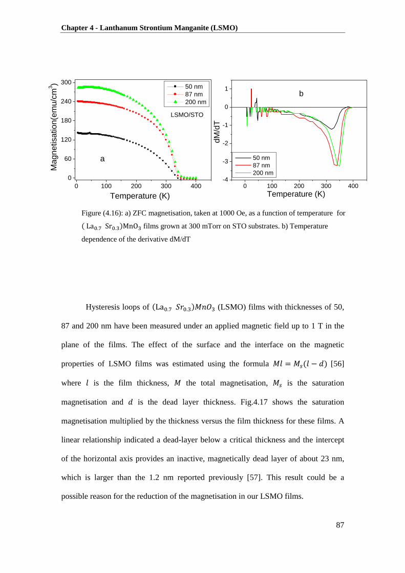
Chapter 4 - Lanthanum Strontium Manganite (LSMO)
87
Hysteresis loops of ( ) (LSMO) films with thicknesses of 50,
87 and 200 nm have been measured under an applied magnetic field up to 1 T in the
plane of the films. The effect of the surface and the interface on the magnetic
properties of LSMO films was estimated using the formula ( ) [56]
where is the film thickness, the total magnetisation, is the saturation
magnetisation and is the dead layer thickness. Fig.4.17 shows the saturation
magnetisation multiplied by the thickness versus the film thickness for these films. A
linear relationship indicated a dead-layer below a critical thickness and the intercept
of the horizontal axis provides an inactive, magnetically dead layer of about 23 nm,
which is larger than the 1.2 nm reported previously [57]. This result could be a
possible reason for the reduction of the magnetisation in our LSMO films.
Figure (4.16): a) ZFC magnetisation, taken at 1000 Oe, as a function of temperature for
( ) films grown at 300 mTorr on STO substrates. b) Temperature
dependence of the derivative dM/dT
0 100 200 300 400-4
-3
-2
-1
0
1b
dM
/dT
Temperature (K)
50 nm
87 nm
200 nm
0 100 200 300 400
0
60
120
180
240
300
a
LSMO/STO
Magne
tisatio
n(e
mu/c
m3)
Temperature (K)
50 nm
87 nm
200 nm
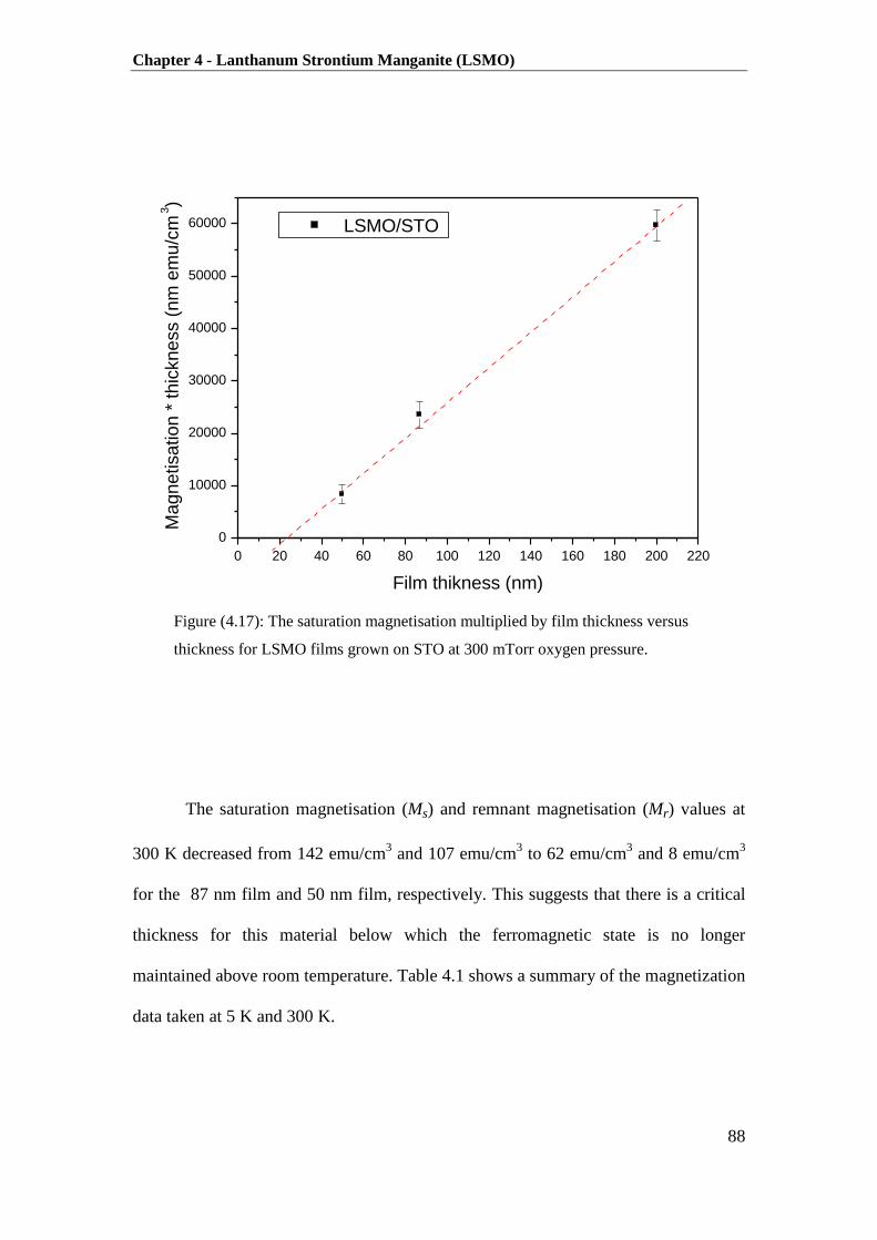
Chapter 4 - Lanthanum Strontium Manganite (LSMO)
88
The saturation magnetisation (Ms) and remnant magnetisation (Mr) values at
300 K decreased from 142 emu/cm3 and 107 emu/cm
3 to 62 emu/cm
3 and 8 emu/cm
3
for the 87 nm film and 50 nm film, respectively. This suggests that there is a critical
thickness for this material below which the ferromagnetic state is no longer
maintained above room temperature. Table 4.1 shows a summary of the magnetization
data taken at 5 K and 300 K.
Figure (4.17): The saturation magnetisation multiplied by film thickness versus
thickness for LSMO films grown on STO at 300 mTorr oxygen pressure.
0 20 40 60 80 100 120 140 160 180 200 220
0
10000
20000
30000
40000
50000
60000
Magnetisation *
thic
kne
ss (
nm
em
u/c
m3)
Film thikness (nm)
LSMO/STO

Chapter 4 - Lanthanum Strontium Manganite (LSMO)
89
Film
thickness
(nm)
Ms(5K)
(emu/cm3)
(5K)
(Oe)
Mr(5K)
(emu/cm3)
Ms(300 K)
(emu/cm3)
(300 K)
(Oe)
Mr(300 K)
(emu/cm3)
50 166 ± 7 284 ± 7 115 ± 5 62 ± 3 9 ± 0.36 8 ± 0.4
87 270 ± 9 38 ± 2 182 ± 8 142 ± 7 22 ± 1.1 107 ± 5
200 298 ± 12 140 ± 6 197 ± 9 142± 7 20 ± 1.2 80 ± 4
Table (4.1): summary of magnetisation data for ( ) films measured at 5 K
and 300 K. Ms denotes the saturation magnetisation, the coercive field and Mr the
remnant magnetisation.
4.3.3 Dependence of Magnetic Properties on Annealing
The as-grown ( ) film, deposited on STO substrate by PLD at
base pressure 4×10⁻³
mTorr, exhibit low saturation magnetisation and low TC. This
might be related to the low oxygen content of the film due to the low oxygen partial
pressure during deposition. It has been found that the oxygen content of LSMO film
could be influenced by the oxygen pressure during the growth [54, 58]. In order to
investigate the effect of annealing on the magnetic properties of LSMO films, the as-
grown films were annealed ex situ at 800 temperatures in air at atmospheric
pressure for one hour. Fig. 4.18 shows ZFC measurement, under in-plane field of
0.1 T for as-grown and annealed LSMO films.

Chapter 4 - Lanthanum Strontium Manganite (LSMO)
90
The magnetisation and TC were enhanced by annealing the as-grown LSMO
film. This is because the LSMO film absorbed oxygen from the air during the
annealing procedures and thus the ratio of Mn4+
/ Mn3+
is increased in the film so that
the ferromagnetic order is enhanced. However, the magnetisation and TC values for
the film grown at low oxygen pressure then annealed in air are below the values of the
film grown at higher oxygen pressure (300 mTorr).
Typical hysteresis loops at 5 K and 300 K for the as-grown and the annealed
LSMO films are plotted in fig.4.19. The coercive fields values at 5 K are 352 and
Figure (4.18): ZFC magnetisation, measured at 1000 Oe, as a function of temperature
of as-grown and annealed ( ) film. The film thickness was 81 nm
grown by PLD on STO substrate.
0 100 200 300 400
0
50
100
150
200
Ma
gn
etisa
tio
n (
em
u/c
m3)
Temperature (K)
LSMO (as-grown)
LSMO ( annealed
at 800 C in air )

Chapter 4 - Lanthanum Strontium Manganite (LSMO)
91
126 Oe while the coercive fields at 300 K are 160 and 25 Oe for the as- grown and
annealed LSMO films, respectively. The coercivities are always lower for the
annealed film than for the as-grown film. This might be related to the presence of
structural defects because the as-grown LSMO film contain more oxygen vacancies,
whereas the annealed LSMO film structure was improved due to the increase of the
oxygen content in the film during the annealing process.
Figure (4.19): Hysteresis loops measured at 5 K and 300 K for as-grown and annealed
( ) films. The film thickness was 81nm; film was grown by PLD on STO
substrate (the diamagnetic contribution from the substrate has been subtracted). The insets show
the enlarged region around the origin.
-10000 -5000 0 5000 10000
-300
-200
-100
0
100
200
300
a
-200 0 200
-20
0
20
Ma
gn
etisa
ion
(e
mu
/cm
3)
Magnetic field (Oe)
5K
as grown
annealed at
800 oC
Magne
tisaio
n (
em
u/c
m3)
Magnetic field (Oe)-10000 -5000 0 5000 10000
-40
-30
-20
-10
0
10
20
30
40
b
-300 0 300
0
Ma
gn
etisa
tio
n(e
mu
/cm
3)
Magnetic field (Oe)
300K
Ma
gn
etisa
tio
n (
em
u/c
m3)
Magnetic field (Oe)
as grown
annealed at
800 oC

Chapter 4 - Lanthanum Strontium Manganite (LSMO)
92
4.3.4 Magneto- Optical Properties of LSMO Thin Films
This section gives measurements of MCD on the ( ) films in
order to obtain information about the polarisation of mobile electrons. The MCD
signal depends on the spin polarisation and electron transition strength. This makes
the MCD a very sensitive tool to study the electronic transition and the nature of
magnetic state in LSMO. Fig. 4.20 shows the MCD spectra of ( )
films as a function of oxygen pressure. These LSMO films were grown on sapphire
substrates at oxygen partial pressures of 4×10⁻³
, 100, 200 and 300 mTorr. The MCD
was recorded at room temperature in fields of up to 1.8 T and in the energy range
1.7 eV to 4.5 eV. The plot shows two main spectral features at 1.7 eV and 3.28 eV.
The spectral feature at 1.7 eV was assigned to a charge transfer excitation from
( ) to the majority–spin (3d Mn) or (
) . The strong peak at
3.28 eV was assigned to an electron excitation 2p (O) to the minority-spin (3d
Mn) band or (
) [10, 50]. The height of the peaks increases with
increase of oxygen growth pressure; this could be attributed to the increase of oxygen
content in the film. A strong peak was found at about 3.28 eV at the highest oxygen
pressure and the peak is found to be shifted to lower energy with decrease of oxygen
pressure. This result could be attributed to the decrease of the Mn4+
fraction and band-
width with reduced oxygen content/pressure. The strength of the peak increased with
increase of the oxygen growth pressure and is related to the ferromagnetic ordering.
The spectral feature at 1.7 eV is broad and is observed in the film with oxygen growth
pressure above 200 mTorr.

Chapter 4 - Lanthanum Strontium Manganite (LSMO)
93
Fig.4.21 shows similar MCD spectra for LSMO films grown on STO substrates.
Once again, two significant spectral features can be distinguished from the plot: one at
1.8 eV and the other at about 3.18 eV. However, The MCD spectra of LSMO films on
STO substrates showed different behaviour from the LSMO spectra on sapphire a
substrate which could be due to the fact that the STO substrate undergoes a structural
transition at 100 K, which gives rise to the birefringence [59]. This is because the
absorption is dominated by the STO absorption edge at higher energies [60] above the
band gap at 3.26 eV as shown in fig.4.22.
Figure (4.20): The MCD spectra at 300 K of ( ) films as a function
of oxygen growth pressure and grown on sapphire substrates.
1.5 2.0 2.5 3.0 3.5 4.0 4.5
-0.04
-0.02
0.00
0.02
0.04
0.06
0.08
0.10
0.12
LSMO/sapphire
MC
D(a
rb.u
nits)
Energy(eV)
base pressure
100 mTorr
200 mTorr
300 mtorr
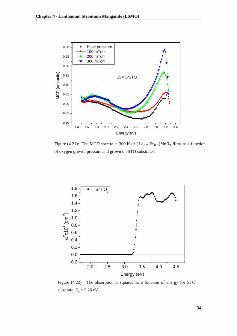
Chapter 4 - Lanthanum Strontium Manganite (LSMO)
94
Figure (4.21): The MCD spectra at 300 K of ( ) films as a function
of oxygen growth pressure and grown on STO substrates,
1.4 1.6 1.8 2.0 2.2 2.4 2.6 2.8 3.0 3.2 3.4
-0.10
-0.05
0.00
0.05
0.10
0.15
0.20
0.25
0.30
LSMO/STO
MC
D (
arb
.un
its)
Energy(eV)
Base pressure
100 mTorr
200 mTorr
300 mTorr
Figure (4.22): The absorption squared as a function of energy for STO
substrate, Eg = 3.26 eV.
2.0 2.5 3.0 3.5 4.0 4.5-0.2
0.0
0.2
0.4
0.6
0.8
1.0
1.2
1.4
1.6
1.8
2x10
4 (
cm
-2)
Energy (eV)
SrTiO3
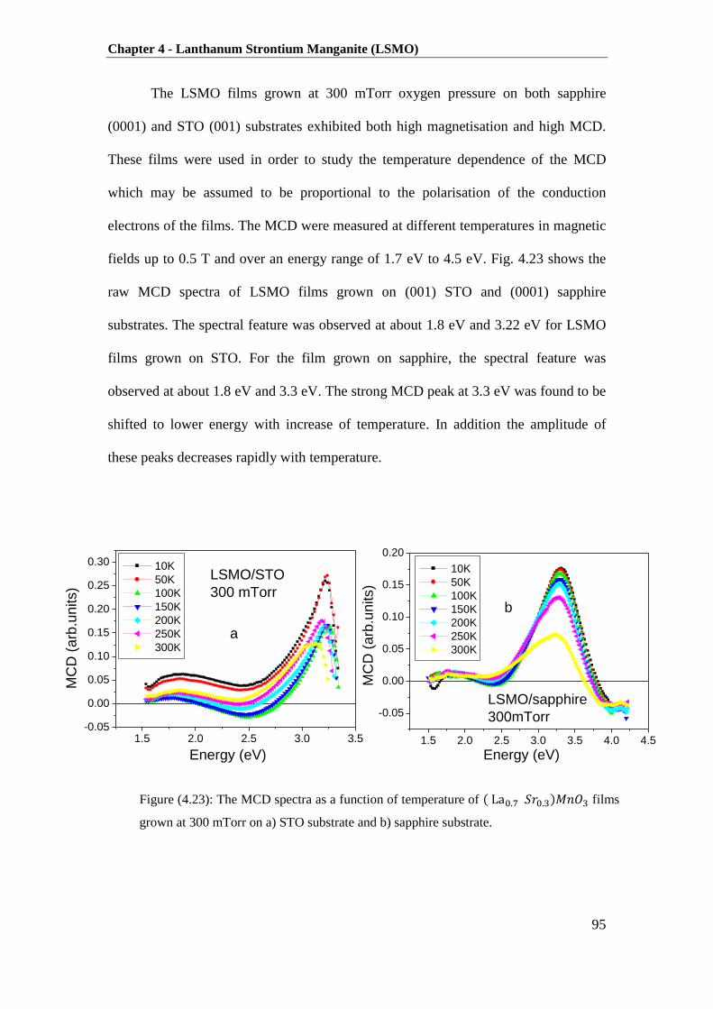
Chapter 4 - Lanthanum Strontium Manganite (LSMO)
95
The LSMO films grown at 300 mTorr oxygen pressure on both sapphire
(0001) and STO (001) substrates exhibited both high magnetisation and high MCD.
These films were used in order to study the temperature dependence of the MCD
which may be assumed to be proportional to the polarisation of the conduction
electrons of the films. The MCD were measured at different temperatures in magnetic
fields up to 0.5 T and over an energy range of 1.7 eV to 4.5 eV. Fig. 4.23 shows the
raw MCD spectra of LSMO films grown on (001) STO and (0001) sapphire
substrates. The spectral feature was observed at about 1.8 eV and 3.22 eV for LSMO
films grown on STO. For the film grown on sapphire, the spectral feature was
observed at about 1.8 eV and 3.3 eV. The strong MCD peak at 3.3 eV was found to be
shifted to lower energy with increase of temperature. In addition the amplitude of
these peaks decreases rapidly with temperature.
Figure (4.23): The MCD spectra as a function of temperature of ( ) films
grown at 300 mTorr on a) STO substrate and b) sapphire substrate.
1.5 2.0 2.5 3.0 3.5-0.05
0.00
0.05
0.10
0.15
0.20
0.25
0.30
a
LSMO/STO
300 mTorr
MC
D (
arb
.un
its)
Energy (eV)
10K
50K
100K
150K
200K
250K
300K
1.5 2.0 2.5 3.0 3.5 4.0 4.5
-0.05
0.00
0.05
0.10
0.15
0.20
b
LSMO/sapphire
300mTorr
MC
D (
arb
.units)
Energy (eV)
10K
50K
100K
150K
200K
250K
300K
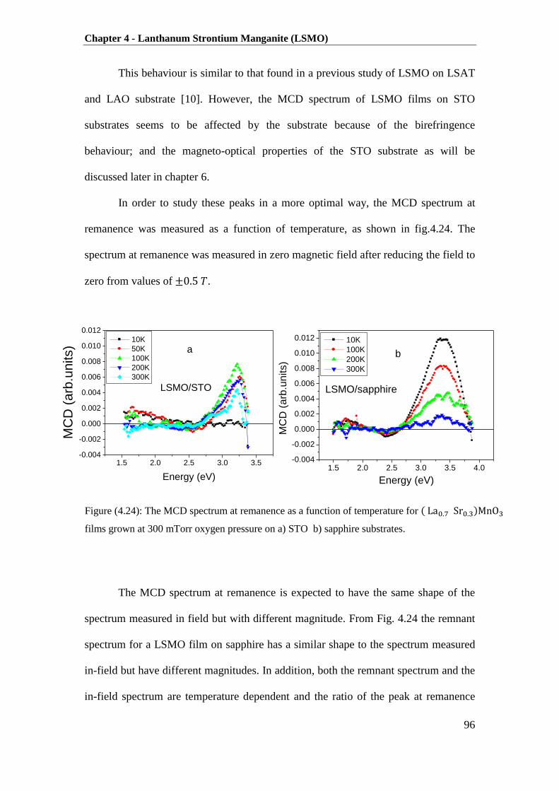
Chapter 4 - Lanthanum Strontium Manganite (LSMO)
96
This behaviour is similar to that found in a previous study of LSMO on LSAT
and LAO substrate [10]. However, the MCD spectrum of LSMO films on STO
substrates seems to be affected by the substrate because of the birefringence
behaviour; and the magneto-optical properties of the STO substrate as will be
discussed later in chapter 6.
In order to study these peaks in a more optimal way, the MCD spectrum at
remanence was measured as a function of temperature, as shown in fig.4.24. The
spectrum at remanence was measured in zero magnetic field after reducing the field to
zero from values of .
The MCD spectrum at remanence is expected to have the same shape of the
spectrum measured in field but with different magnitude. From Fig. 4.24 the remnant
spectrum for a LSMO film on sapphire has a similar shape to the spectrum measured
in-field but have different magnitudes. In addition, both the remnant spectrum and the
in-field spectrum are temperature dependent and the ratio of the peak at remanence
Figure (4.24): The MCD spectrum at remanence as a function of temperature for ( )
films grown at 300 mTorr oxygen pressure on a) STO b) sapphire substrates.
1.5 2.0 2.5 3.0 3.5-0.004
-0.002
0.000
0.002
0.004
0.006
0.008
0.010
0.012
a
LSMO/STO
MC
D (
arb
.units)
Energy (eV)
10K
50K
100K
200K
300K
1.5 2.0 2.5 3.0 3.5 4.0-0.004
-0.002
0.000
0.002
0.004
0.006
0.008
0.010
0.012
b
LSMO/sapphire
MC
D (
arb
.un
its)
Energy (eV)
10K
100K
200K
300K

Chapter 4 - Lanthanum Strontium Manganite (LSMO)
97
and in-field is comparable to the ratio of Mr/Ms observed in the SQUID data at 300 K
shown in fig.4.15. On the other hand, the shape of the remnant spectrum for the
LSMO film grown on STO is unlike to the shape of the MCD spectrum measured in-
field. Furthermore, the peak at about 3 eV has a minimum value at 10 K and a
maximum value at 100 K; the peak then subsequently decreased with increasing
temperature. This is extremely good evidence that this peak is affected by the
contribution from the STO substrate. This could be related to the fact that STO has a
cubic perovskite structure at room temperature, but undergoes a structural transition to
a tetragonal phase at about 100 K which gives rise to a birefringence. Moreover, the
birefringence is linearly dependent on temperature and decrease with increase of
temperature, and the birefringence falls to zero at about 100 K [37, 59]. In addition,
for the LSMO film grown on STO, the peak at about 3 eV is found to be shifted to
lower energy, compared to the film on sapphire. In summary, the MCD spectrum of
the LSMO film on STO was dominated by the birefringence and the magneto optical
properties arising from the STO substrate. Consequently, the STO substrate was then
studied carefully with a regard to the orientation of the substrate; this will be
discussed in chapter 6.
Fig.4.25 shows a comparative study of Magnetisation temperature dependence
and MCD temperature dependence for both LSMO films grown on STO and sapphire
substrates. The magnetisation data obtained from the SQUID using ZFC
measurements in a field of 0.1 T. The SQUID data were normalized with
magnetisation at 5K and the MCD data were normalized with data at 10 K. The MCD
signal follows the magnetisation for the LSMO film grown on sapphire, but shows
different behaviour for LSMO film grown on STO. This result displayed very good
evidence that the conduction electrons follow the magnetisation for LSMO films

Chapter 4 - Lanthanum Strontium Manganite (LSMO)
98
grown on sapphire substrate, but for LSMO films grown on STO the MCD data was
dominated by birefringence and the magneto-optical properties arising from the STO
substrate. The anomaly in the MCD data at 100 K compared with SQUID data in
fig.4.24a is due to the birefringence arising from the structural transition of the STO
substrate.
Figure (4.25): Temperature dependence of M(T)/M (5K) and MCD(T)/MCD(10K) of
( ) films grown at 300 mTorr on a) STO and b) sapphire substrates.
0 100 200 300 400-0.2
0.0
0.2
0.4
0.6
0.8
1.0
b
LSMO/sapphire
300mTorr
Ms(T
)/M
s(5
K)
, M
CD
(T)/
MC
D(1
0K
)
Temperature(K)
SQUID
MCD
0 100 200 300 400
0.0
0.2
0.4
0.6
0.8
1.0
a
LSMO/STO
300mTorr
Ms(T
)/M
S(5
K),
MC
D(T
)/M
CD
(10K
)
Temperature (K)
SQUID
MCD

Chapter 4 - Lanthanum Strontium Manganite (LSMO)
99
4.4 Summary and Conclusions
This chapter reported results of the investigation of the magnetic and magneto-
optical properties of ( ) thin films deposited under different growth
conditions. LSMO thin films were deposited successfully by PLD on (001) STO and
(0001) sapphire substrates. The films were prepared with various concentrations
( =0.15, 0.30 and 0.50) and various oxygen pressures. The LSMO films grown on
STO and sapphire substrate show a pronounced hysteresis loops at 300 and 5 K,
which verify that LSMO maintains strong ferromagnetic properties at room
temperature and this is consistent with previous studies. The films grown with 30% of
Sr on both STO and sapphire substrates exhibited higher magnetisation and the
magnetisation increased with increase of oxygen pressure.
The MCD spectral feature was observed at about 1.7 eV and 3.28 eV for
( ) films grown at different oxygen pressures on sapphire substrates.
The strong MCD peak at 3.28 eV was found to be shifted to lower energy with
decreasing oxygen pressure; this could be attributed to the decrease of the Mn4+
fraction and band width with reduced oxygen. The temperature dependence of the
MCD spectra displayed peaks at 1.8 eV and 3.3 eV for ( ) films
grown at 300 mTorr oxygen pressure on sapphire substrates. The strong MCD peak at
3.3 eV was found to be shifted to lower energy with increase of temperature and the
strength of these peaks weakens rapidly with temperature. The MCD spectra of
LSMO films on STO substrates seems to be dominated by the magneto-optical
properties and birefringence behaviour arising from the STO substrate. The MCD
signal follows the magnetisation for the LSMO film grown on sapphire, but shows a
different behaviour for LSMO film grown on STO.

Chapter 4 - Lanthanum Strontium Manganite (LSMO)
100
Overall, STO substrate was chosen because it suitable for the growth of high
quality epitaxial thin films. However, this did have some disadvantages for an optical
study. The band gap energy at 3.2 eV was unfortunate; it reduced the useful energy
range over which absorption of the films could be measured. However, another
disadvantage was the structural transition at ~100 K, which gives rise to a
birefringence, unless the E vector of the light is along an optic axis. The magneto-
optical data of LSMO on sapphire substrates are significantly better than LSMO
grown on STO substrates. This makes sapphire an optimal substrate for the growth of
LSMO.
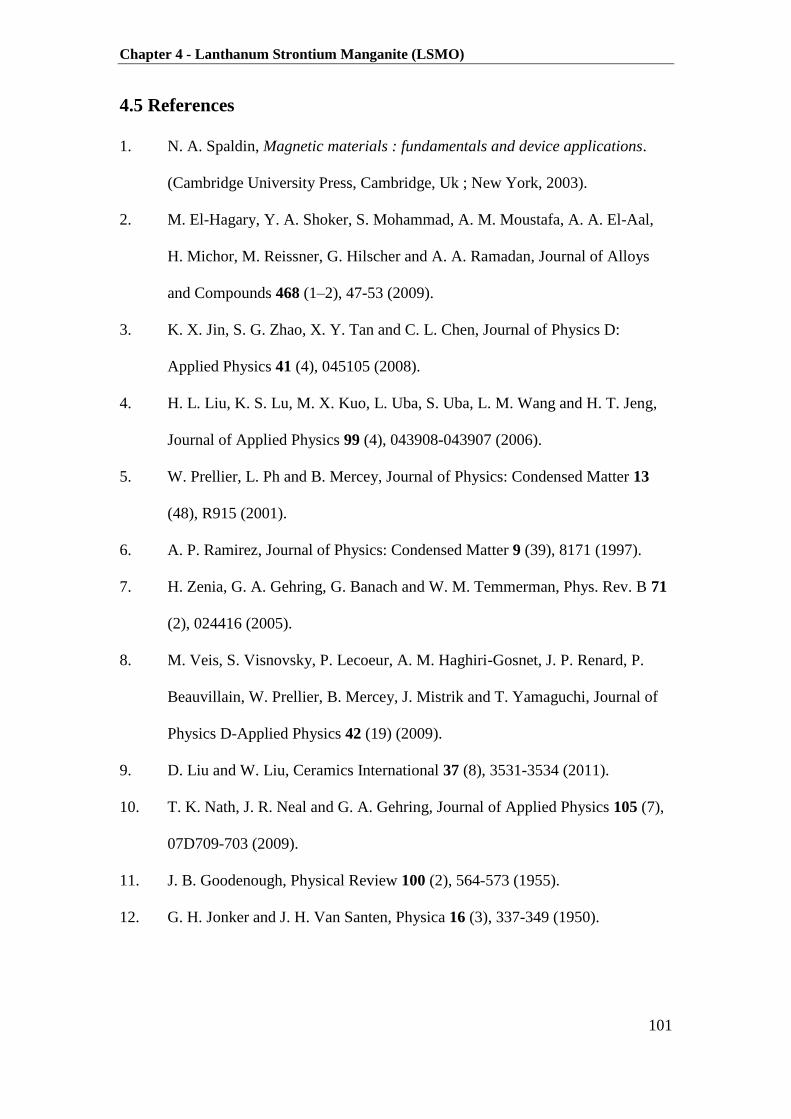
Chapter 4 - Lanthanum Strontium Manganite (LSMO)
101
4.5 References
1. N. A. Spaldin, Magnetic materials : fundamentals and device applications.
(Cambridge University Press, Cambridge, Uk ; New York, 2003).
2. M. El-Hagary, Y. A. Shoker, S. Mohammad, A. M. Moustafa, A. A. El-Aal,
H. Michor, M. Reissner, G. Hilscher and A. A. Ramadan, Journal of Alloys
and Compounds 468 (1–2), 47-53 (2009).
3. K. X. Jin, S. G. Zhao, X. Y. Tan and C. L. Chen, Journal of Physics D:
Applied Physics 41 (4), 045105 (2008).
4. H. L. Liu, K. S. Lu, M. X. Kuo, L. Uba, S. Uba, L. M. Wang and H. T. Jeng,
Journal of Applied Physics 99 (4), 043908-043907 (2006).
5. W. Prellier, L. Ph and B. Mercey, Journal of Physics: Condensed Matter 13
(48), R915 (2001).
6. A. P. Ramirez, Journal of Physics: Condensed Matter 9 (39), 8171 (1997).
7. H. Zenia, G. A. Gehring, G. Banach and W. M. Temmerman, Phys. Rev. B 71
(2), 024416 (2005).
8. M. Veis, S. Visnovsky, P. Lecoeur, A. M. Haghiri-Gosnet, J. P. Renard, P.
Beauvillain, W. Prellier, B. Mercey, J. Mistrik and T. Yamaguchi, Journal of
Physics D-Applied Physics 42 (19) (2009).
9. D. Liu and W. Liu, Ceramics International 37 (8), 3531-3534 (2011).
10. T. K. Nath, J. R. Neal and G. A. Gehring, Journal of Applied Physics 105 (7),
07D709-703 (2009).
11. J. B. Goodenough, Physical Review 100 (2), 564-573 (1955).
12. G. H. Jonker and J. H. Van Santen, Physica 16 (3), 337-349 (1950).

Chapter 4 - Lanthanum Strontium Manganite (LSMO)
102
13. A. K. Pradhan, D. Hunter, T. Williams, B. Lasley-Hunter, R. Bah, H. Mustafa,
R. Rakhimov, J. Zhang, D. J. Sellmyer, E. E. Carpenter, D. R. Sahu and J. L.
Huang, Journal of Applied Physics 103 (2), 023914-023918 (2008).
14. J. M. D. Coey, M. Viret and S. von Molnár, Advances in Physics 48 (2), 167-
293 (1999).
15. J. M. D. Coey, M. Viret, L. Ranno and K. Ounadjela, Physical Review Letters
75 (21), 3910-3913 (1995).
16. J. G.H, Physica 22 (6–12), 707-722 (1956).
17. M. M. Savosta, P. Novák and Z. Jirák, Phys. Rev. B 67 (10), 100411 (2003).
18. E. Dagotto, T. Hotta and A. Moreo, Physics Reports-Review Section of
Physics Letters 344 (1-3), 1-153 (2001).
19. H. Kuwahara, Y. Tomioka, A. Asamitsu, Y. Moritomo and Y. Tokura, Science
270 (5238), 961-963 (1995).
20. M. B. Salamon and M. Jaime, Reviews of Modern Physics 73 (3), 583-628
(2001).
21. Y. Tokura and Y. Tomioka, J. Magn. Magn. Mater. 200 (1-3), 1-23 (1999).
22. A. Urushibara, Y. Moritomo, T. Arima, A. Asamitsu, G. Kido and Y. Tokura,
Phys. Rev. B 51 (20), 14103-14109 (1995).
23. J. F. Lawler, J. G. Lunney and J. M. D. Coey, Applied Physics Letters 65 (23),
3017-3018 (1994).
24. J. M. D. Coey and S. Sanvito, Journal of Physics D: Applied Physics 37 (7),
988 (2004).
25. J. M. D. Coey and M. Venkatesan, Journal of Applied Physics 91 (10), 8345-
8350 (2002).
26. C. Zener, Physical Review 81 (3), 440-444 (1951).

Chapter 4 - Lanthanum Strontium Manganite (LSMO)
103
27. C. Zener, Physical Review 82 (3), 403-405 (1951).
28. A. Tebano, C. Aruta, S. Sanna, P. G. Medaglia, G. Balestrino, A. A.
Sidorenko, R. De Renzi, G. Ghiringhelli, L. Braicovich, V. Bisogni and N. B.
Brookes, Physical Review Letters 100 (13), 137401 (2008).
29. M. Opel, Journal of Physics D-Applied Physics 45 (3) (2012).
30. A. M. Haghiri-Gosnet and J. P. Renard, Journal of Physics D: Applied Physics
36 (8), R127 (2003).
31. M. Cesaria, A. P. Caricato, G. Maruccio and M. Martino, Journal of Physics:
Conference Series 292 (1), 012003 (2011).
32. J. F. Mitchell, D. N. Argyriou, C. D. Potter, D. G. Hinks, J. D. Jorgensen and
S. D. Bader, Phys. Rev. B 54 (9), 6172-6183 (1996).
33. M. L. Wilson, J. M. Byers, P. C. Dorsey, J. S. Horwitz, D. B. Chrisey and M.
S. Osofsky, Journal of Applied Physics 81 (8), 4971-4973 (1997).
34. A. I. Tovstolytkin, A. N. Pogorily, A. I. Matviyenko, A. Y. Vovk and Z.
Wang, Journal of Applied Physics 98 (4), 043902-043906 (2005).
35. R. Desfeux, S. Bailleul, A. Da Costa, W. Prellier and A. M. Haghiri-Gosnet,
Applied Physics Letters 78 (23), 3681-3683 (2001).
36. S. Mukhopadhyay, I. Das and S. Banerjee, Journal of Physics-Condensed
Matter 21 (2) (2009).
37. D. Pesquera, V. Skumryev, F. Sánchez, G. Herranz and J. Fontcuberta, Phys.
Rev. B 84 (18), 184412 (2011).
38. V. Garcia, M. Bibes, A. Barthélémy, M. Bowen, E. Jacquet, J. P. Contour and
A. Fert, Phys. Rev. B 69 (5), 052403 (2004).

Chapter 4 - Lanthanum Strontium Manganite (LSMO)
104
39. C. Kwon, M. C. Robson, K. C. Kim, J. Y. Gu, S. E. Lofland, S. M. Bhagat, Z.
Trajanovic, M. Rajeswari, T. Venkatesan, A. R. Kratz, R. D. Gomez and R.
Ramesh, J. Magn. Magn. Mater. 172 (3), 229-236 (1997).
40. C. Thiele, K. Dörr, O. Bilani, J. Rödel and L. Schultz, Phys. Rev. B 75 (5),
054408 (2007).
41. F. Yang, N. Kemik, M. D. Biegalski, H. M. Christen, E. Arenholz and Y.
Takamura, Applied Physics Letters 97 (9), 092503-092503 (2010).
42. S. M. Liu, X. B. Zhu, J. Yang, W. H. Song, J. M. Dai and Y. P. Sun, Ceramics
International 32 (2), 157-162 (2006).
43. V. Bhosle and J. Narayan, Applied Physics Letters 90 (10), 101903-101903
(2007).
44. H. Y. Hwang, S. W. Cheong, N. P. Ong and B. Batlogg, Physical Review
Letters 77 (10), 2041-2044 (1996).
45. R. Mahesh, R. Mahendiran, A. K. Raychaudhuri and C. N. R. Rao, Applied
Physics Letters 68 (16), 2291-2293 (1996).
46. M. Jaime, M. B. Salamon, K. Pettit, M. Rubinstein, R. E. Treece, J. S. Horwitz
and D. B. Chrisey, Applied Physics Letters 68 (11), 1576-1578 (1996).
47. H. L. Ju, C. Kwon, Q. Li, R. L. Greene and T. Venkatesan, Applied Physics
Letters 65 (16), 2108-2110 (1994).
48. D. W. Visser, A. P. Ramirez and M. A. Subramanian, Physical Review Letters
78 (20), 3947-3950 (1997).
49. Y. P. Sukhorukov, A. M. Moskvin, N. N. Loshkareva, I. B. Smolyak, V. E.
Arkhipov, Y. M. Mukovskii and A. V. Shmatok, Technical Physics 46 (6),
778-781 (2001).

Chapter 4 - Lanthanum Strontium Manganite (LSMO)
105
50. S. Yamaguchi, Y. Okimoto, K. Ishibashi and Y. Tokura, Phys. Rev. B 58 (11),
6862-6870 (1998).
51. E. O. Wollan and W. C. Koehler, Physical Review 100 (2), 545-563 (1955).
52. E. Pellegrin, L. H. Tjeng, F. M. F. deGroot, R. Hesper, G. A. Sawatzky, Y.
Moritomo and Y. Tokura, Journal of Electron Spectroscopy and Related
Phenomena 86 (1-3), 115-118 (1997).
53. Y. P. Sukhorukov, A. P. Nosov, N. N. Loshkareva, E. V. Mostovshchikova, A.
V. Telegin, E. Favre-Nicolin and L. Ranno, Journal of Applied Physics 97
(10), 103710-103715 (2005).
54. Y. S. Du, B. Wang, T. Li, D. B. Yu and H. Yan, J. Magn. Magn. Mater. 297
(2), 88-92 (2006).
55. M. Pardavihorvath, IEEE Trans. Magn. 21 (5), 1694-1699 (1985).
56. S. K. Arora, H.-C. Wu, R. J. Choudhary, I. V. Shvets, O. N. Mryasov, H. Yao
and W. Y. Ching, Phys. Rev. B 77 (13), 134443 (2008).
57. M. Huijben, L. W. Martin, Y. H. Chu, M. B. Holcomb, P. Yu, G. Rijnders, D.
H. A. Blank and R. Ramesh, Phys. Rev. B 78 (9) (2008).
58. H. Boschker, M. Huijben, A. Vailionis, J. Verbeeck, S. van Aert, M.
Luysberg, S. Bals, G. van Tendeloo, E. P. Houwman, G. Koster, D. H. A.
Blank and G. Rijnders, Journal of Physics D-Applied Physics 44 (20) (2011).
59. M. A. Geday and A. M. Glazer, Journal of Physics-Condensed Matter 16 (20),
3303-3310 (2004).
60. K. van Benthem, C. Elsasser and R. H. French, Journal of Applied Physics 90
(12), 6156-6164 (2001).

Chapter 5 – Multiferroic manganite GdMnO3
106
Chapter 5
Multiferroic Manganite GdMnO3
5.1 Introduction
In recent years, multiferroic materials have attracted much attention due to
both their physical properties and their promising applications. Multiferroic materials
exhibit ferroelectric and ferromagnetic properties simultaneously in the same phase.
This allows one to control the electric polarisation by the application of a magnetic
field or, vice versa, to control the magnetic properties by an electric field. Together
with recent unprecedented progress in epitaxial thin film growth, this unique property
makes these well-known materials very good candidates with which to build
multifunctional spintronic devices [2-3].
Currently, the heart of the problem is to find examples of muliferroic
materials. The coupling of both ferroelectric and ferromagnetic properties in a
multiferroic can be controlled indirectly through the strain [4]. This phenomenon in
multiferroic materials is the key to developing novel spintronic devices. However,
these novel devices require a very high quality of thin film, rather than bulk material,
this requirement being the central challenge for the researcher. Probably the most
promising class of multiferroic materails are the perovskite manganites, RMnO3,
where R is a rare-earth element or bismuth (R=Ho, Er, Tm, La, Sm, Gd,…..) [4-6]. In
this chapter we shall study the magnetic, optical and magneto-optical properties of
epitaxial films of gadolinium manganite (GdMnO3) in order to obtain detailed
information on the magnetic polarisation of the electronic states. The first section of

Chapter 5 – Multiferroic manganite GdMnO3
107
this chapter provides a literature review of multiferroic materials and the second
section investigates the magnetic and magneto-optical properties. The data presented
in this chapter have been accepted for publication.
5.2 Literature Review on the Multiferroic, Gadolinium Manganite
(GdMnO3)
The study of multiferroic materials began in the 1960’s by Smolenskii and
Venevtsev in the then Soviet Union [7]. This field was very quiet for some time, and
renewed interest in multiferroics started around 2001-2003. In recent years, the rare-
earth manganites (RMnO3) have been found to have large magneto-electric effects [7-
9]. This makes the perovskite manganites (RMnO3) very promising multiferroic
materials. with regard to the structure, these manganites can be classified into two
groups: a hexagonal phase with R (= Ho, Er , Tm, Yb or Y) and an orthorhombic
phase with R (= La, Pr, Nd, Sm, Eu, Gd,Tb or Dy) [9]. However, some compounds in
the orthorhombic group could be grown in a metastable hexagonal phase and vice
versa. This could be achieved by an epitaxial stabilization technique, which required
high oxygen pressure and a suitable substrate [10-12].
On lowering the temperature, most of the hexagonal RMnO3 manganites
display three kind of magnetic ordering transitions: -oriented antiferromagnetic
at 70-85 K, rotation of Mn3+
spins, known as reorientation transition, at 40 K and
ferromagnetic ordering below 5K due to the magnetic interaction between rare-earth
ions [10, 13-14]. In the structure of hexagonal manganites, the ferroelectric and
magnetic ordering do not occur together, since the electric polarization appears far
above room temperature and the magnetism appears below this temperature [8, 15]. In

Chapter 5 – Multiferroic manganite GdMnO3
108
contrast, the magnetic and the ferroelectric ordering transition temperatures are
comparable for manganites with orthorhombic structure [8, 16-17].
The orthorhombic structures occur where the lanthanide ions have a large
ionic radius, whereas hexagonal structures occur where the lanthanide ions have a
small ionic radius. A decrease of rare-earth ionic radius (rR) in orthorhombic
manganites RMnO3 enhances the competition in magnetic interaction [1]. The FM
interaction occurs between nearest-neighbour Mn ion and the AF interaction occurs
between next-nearest neighbour ions [1, 18].
T.Kimura et al reported [1] the magnetic phase diagram for the orthorhombic
manganites RMnO3 as a function of ionic radius as indicated in fig.5.1.
Removed by the
author for copyright reasons
Figure (5.1): The magnetic phase diagram of RMnO3 as a function of ionic radius R.
The open triangles denote the Néel temperature for Mn moments TN (Mn), closed
triangles denote the lock-in transition temperature Tlock and cross the Néel
temperature for R moments TN(R) [1].

Chapter 5 – Multiferroic manganite GdMnO3
109
The Néel temperature (TN) increases with increasing ionic radius, where TN for
GdMnO3 is about 43 K and the lock-in temperature (Tlock) about 23 K. Tlock is the
temperature at which the ferroelectric polarisation vector is switched from being
directed along a given axis to a different axis by the application of a magnetic field
[17]. Among R3+
4f ions in rare-earth manganites RMnO3, the Gd3+
ion in GdMnO3
has a large effective spin moment (S=7/2) and large g[J(J+1)]1/2
factor. These two
properties could give a significant enhancement of ferromagnetic properties in
GdMnO3 [10].
The magnetic transitions in the orthorhombic manganites RMnO3 is currently
understood with the help of two key ingredients. Firstly, magnetic frustration due to
competing exchange integrals between successive neighbours stabilizes a spiral
magnetic phase below the TN [17, 19]. Secondly, there is a lock-in transition to a
canted A-type antiferromagnetic phase. At lower temperature still the Gd moments
order and the oxygen atoms are pushed off the Mn-Mn bond, driving an electric
polarisation at this transition for GdMnO3. Therefore, the charge, spin orbital and
lattice subsystems are linked very tightly in these materials and the strain in the thin
films plays a crucial role in determining the properties of the materials.
The magnetic phase diagram (H-T) has been mapped out for bulk crystals [20-
21] as a function of temperature and magnetic field. It was found that the H-T phases
are field-orientation dependent along the a, b and c axes. As shown in fig.5.2 the
transition from the paramagnetic (PM) to an incommensurate antiferromagnetic
(ICAFM) occurs with around TN=42 K. The transition from (ICAFM) to a canted A-
type antiferromagnet (cAFM) and a transition to ferroelectric (FE) occurs at Tc=20 K
and 12 K, respectively for magnetic fields above 2 T.

Chapter 5 – Multiferroic manganite GdMnO3
110
Removed by the
author for copyright reasons
Figure (5.2): Phase diagram of GdMnO3 for magnetic field along the b axis. Closed and open
symbols are obtained with increasing and decreasing T or H, respectively. Shaded areas
indicate regions of strong hysteresis [8].
It was found that, as the temperature is lowered, the spiral magnetic order in
GdMnO3 occurs at TN=47 K and there is a transition between the paramagnetic phase
and an antiferromagnetic phase and an A-type antiferromagnetic transition at 19 K [8,
17, 22]. In zero field there is a transition to a canted phase at about 18 K and the Gd
spins order at close to 7 K. However, below 20 K there is strong hysteresis so that
several phases can co-exist [21]. The phase boundaries depend both on the magnitude
of the magnetic field and its direction. In particular a ferroelectric phase appears
below 7 K for magnetic fields greater than 2 T along the b axis. The phase diagram is
very dependent on pressure [8, 22], as expected due to the existence of a ferroelectric
phase. The first phase transition was found to be shifted to 44 K for nanoparticles with
a mean size of 52 nm [23] as indicated in fig.5.3. Weak ferromagnetism appears in FC
mode at 20 K, which is attributed to the canted Mn spins and polarisation of Gd 4f

Chapter 5 – Multiferroic manganite GdMnO3
111
spins. At 7 K, the canted Gd spins are antiparallel to those of the canted Mn spins, due
to the interaction of Gd 4f spins. Moreover, a ferromagnetic-like loop was reported at
2 K for GdMnO3 nanoparticles [23] this is due to large contribution of the net moment
of Gd spins compared to that of the antiferromagnetic canted Mn spins.
Removed by the
author for copyright reasons
Figure (5.3): ZFC and FC magnetisation of GdMnO3 nanoparticles measured in 100 Oe
between 2 and 60 K. The inset is the temperature dependence of the derivative dM/dT [23].
The optical absorption spectra for rare-earth manganite RMnO3 including
GdMnO3 show a strong transition at the 3.53 eV band edge. However, in LaMnO3 a
particular interesting feature is seen at about 2 eV as is shown in fig.5.4. This clear
peak is due to a charge transfer excitation between neighbouring Mn ions; the
reduction in the intensity has been related to the different canting of the Mn d-orbitals

Chapter 5 – Multiferroic manganite GdMnO3
112
and also on the directions of Mn spins and the Mn-O-Mn bond angle [24-25]. The
only magneto- optical studies on a related material reported a strong magnetic field
dependent peak at near 3 eV in single-crystal of TbMnO3 [26].
Removed by the
author for copyright reasons
Figure (5.4): Absorption spectra of RMnO3 thin films measured at room temperature shows a
transition peak at 2 eV being suppressed for Gd and Tb [25].

Chapter 5 – Multiferroic manganite GdMnO3
113
5.3 Experimental Results and Discussion
The GdMnO3 target was prepared from a high-purity stoichiometric mixture of
Gd2O3 and MnO2 powders. Films were grown by Ya. Mukovski in the laboratory of
the National University of Science and Technology, Moscow, Russia. The films were
sputtered in an atmosphere of Ar and O2 at a pressure of 1-2 mTorr. The substrate
temperature was maintained at 650 during the growth process. Epitaxial films of
thickness 100-200 nm were grown on LaAlO3 (LAO) and SrTiO3 (STO) substrates
with the [110]-direction parallel to the plane of the substrate. X-ray diffraction (XRD)
was also used to study the structure of the films, as shown in fig.5.5.
Fig.5.5 shows XRD patterns taken at room temperature for the GdMnO3 films
grown on the STO and LAO substrates. The data indicates an epitaxial growth for
both films with films oriented with the substrates. The strong reflection peak at
2 = 47o is corresponds to the (431) GdMnO3 orientation. The LAO was found to be
heavily twinned and the STO substrate undergoes a structural transition at about
Figure (5.5): X-ray data of GdMnO3 films grown on STO3 and LAO substrate.

Chapter 5 – Multiferroic manganite GdMnO3
114
100K; this may produce further strains on the film in the temperature range where the
magnetic ordering occurs.
5.3.1 Magnetic Measurements
Magnetic properties of the GdMnO3 films were investigated using the SQUID
magnetometer. Measurement was made in the temperature range of 5-400 K with a
field up to 1 T in-plane. FC and (ZFC) measurement was achieved in a field of 0.01 T.
Fig.5.6 shows the ZFC and FC magnetization of GdMnO3 films after the contribution
from the substrates has been subtracted.
The transition to the antiferromagnetic phase shows up most clearly in the
ZFC plots; however it is shifted to lower temperature. For the films on the STO
substrate, it occurs at 44 K and for the film on LAO substrate 40 K. These should be
compared with the temperature of 44 K observed for GdMnO3 nanoparticles [23] and
47 K in bulk material. This indicates that the strain induced by the substrate is
Fig.5.6: ZFC and FC data taken in an in-plane field of 100 Oe for films of GdMnO3 on
a) STO and b) LAO substrates. The data for the bare substrate has been subtracted.
0 50 100 150 200 250 3000.0
5.0x10⁻⁶
1.0x10⁻⁵
1.5x10⁻⁵
2.0x10⁻⁵
2.5x10⁻⁵
3.0x10⁻⁵
b
Magnetic m
om
ent
(em
u)
Temperature (K)
ZFC
FC
100Oe
0 50 100 150 200 250 3000.0
5.0x10⁻⁶
1.0x10⁻⁵
1.5x10⁻⁵
2.0x10⁻⁵
2.5x10⁻⁵
3.0x10⁻⁵
a
Ma
gne
tic m
om
en
t (e
mu
)
Temperature (K)
ZFC
FC
100Oe

Chapter 5 – Multiferroic manganite GdMnO3
115
significant in reducing TN. Moreover, the exchange interactions between the Mn ions
are very sensitive to strain [17].
Fig.5.7 shows the temperature dependence of the inverse susceptibility taken
from both the FC and ZFC measurements. There are small changes in the slope of the
inverse susceptibility, which are marked with arrows on the plots. These occur at 14 K
for both films; this is tentatively identified as the lock-in temperature. There is an
additional, weak change of slope at 8 K for the film on STO, which is identified as the
ordering temperature of the Gd ions; another weak feature also occurs at 108 K,
which is the temperature of the structural transition in the STO substrate.
The slope of the inverse susceptibility is extrapolated to give the Curie-Weiss
constant. This gives a value of 7.5±0.23 K and 8.5±0.30 K for the films on the STO
and LAO respectively. The slope of the line is the inverse Curie constant, which is
expected to arise from the paramagnetic Gd spins and a weakly temperature
Figure (5.7): The inverse susceptibilities, evaluated from both the FC and ZFC data are
plotted as a function of temperature for the films on (a) STO and (b) LAO substrates. The
magnetic transitions are marked on these plots.
-40 -20 0 20 40 60 80 100 120
0.0
5.0x10⁶
1.0x10⁷
1.5x10⁷
2.0x10⁷
2.5x10⁷
3.0x10⁷
b
GdMnO3/LaAlO
3
8.5K
40K
14K
Invers
e s
usceptibili
ty
Temperature(K)
ZFC
Fc
-40 -20 0 20 40 60 80 100 120
0.0
4.0x10⁶
8.0x10⁶
1.2x10⁷
1.6x10⁷
2.0x10⁷
a
7.5K
14K
8K
44K
108K
GdMnO3/SrTiO
3
Invers
e s
uscptib
ility
Temperature (K)
ZFC
FC

Chapter 5 – Multiferroic manganite GdMnO3
116
dependent susceptibility from the Mn ions. The expected paramagnetic
susceptibility from Gd ions was calculated using:
, 5.1
where, N is the number of Gd ions per cm3
in the film, the Bohr
magnetons, the electron spin, s=7/2 and g=2; the total susceptibility is then given as:
5.2
The measured values of the Curie constant for the FC and ZFC plots
for both films and the calculated value of Gd ions (C (Gd)) are given in Table (5.1).
The experimental are higher than the calculated values for Gd ions (C (Gd))
which is good evidence for the canted antiferromagnetic contribution from the Mn
ions; this is enhanced with magnetic field.
The film 6(Gd) 10C 610
meas
zfcC 610
meas
fcC
GdMnO3 on STO 1.13 2.55 3.77
GdMnO3 on ALO 1.13 3.41 3.82
Tale (5.1): shows the calculated and the measured values of the Curie constant for GdMnO3
films grown on STO and ALO substrates. C (Gd) denote the Curie constant values calculated
for Gd ions,
the Curie constant values measured from ZFC and
the Curie
constant values measured from FC.
The magnetisation hysteresis loops of the GdMnO3 films grown on STO and
LAO substrate were measured under an applied magnetic field up to 1 T parallel to
the surface of all films. The contribution from the substrates, that varied linearly with
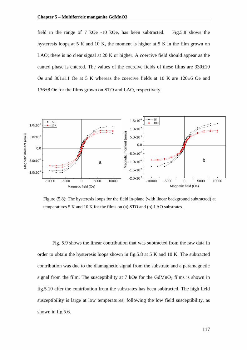
Chapter 5 – Multiferroic manganite GdMnO3
117
-10000 -5000 0 5000 10000
-1.0x10⁻⁴
-5.0x10⁻⁵
0.0
5.0x10⁻⁵
1.0x10⁻⁴
a
Magnetic m
om
ent
(em
u)
Magnetic field (Oe)
5K
10K
field in the range of 7 kOe -10 kOe, has been subtracted. Fig.5.8 shows the
hysteresis loops at 5 K and 10 K, the moment is higher at 5 K in the film grown on
LAO; there is no clear signal at 20 K or higher. A coercive field should appear as the
canted phase is entered. The values of the coercive fields of these films are 330±10
Oe and 301±11 Oe at 5 K whereas the coercive fields at 10 K are 120±6 Oe and
136±8 Oe for the films grown on STO and LAO, respectively.
Fig. 5.9 shows the linear contribution that was subtracted from the raw data in
order to obtain the hysteresis loops shown in fig.5.8 at 5 K and 10 K. The subtracted
contribution was due to the diamagnetic signal from the substrate and a paramagnetic
signal from the film. The susceptibility at 7 kOe for the GdMnO3 films is shown in
fig.5.10 after the contribution from the substrates has been subtracted. The high field
susceptibility is large at low temperatures, following the low field susceptibility, as
shown in fig.5.6.
-10000 -5000 0 5000 10000-2.0x10
-4
-1.5x10⁻⁴
-1.0x10⁻⁴
-5.0x10⁻⁵
0.0
5.0x10⁻⁵
1.0x10⁻⁴
1.5x10⁻⁴
b
Magnetic m
om
ent
(em
u)
Magnetic field (Oe)
5K
10K
Figure (5.8): The hysteresis loops for the field in-plane (with linear background subtracted) at
temperatures 5 K and 10 K for the films on (a) STO and (b) LAO substrates.

Chapter 5 – Multiferroic manganite GdMnO3
118
Figure (5.9): The linear contribution that was subtracted from the raw date to obtain the
correcte loops for the films (a) on the STO substrate (b) on the LAO substrate.
0 20 40 60 80 100
0.0
6.0x10⁻⁸
1.2x10⁻⁷
1.8x10⁻⁷
b
GdMnO3/LaAlO
3
Suscptibili
ty
Temperature (K)
Figure (5.10): The susceptibility at 7 kOe for the GdMnO3 (a) on the STO substrate (b) on
the LAO substrate. The contribution from the substrates has been subtracted.
-10000 -5000 0 5000 10000
-6.0x10⁻⁴
-4.0x10⁻⁴
-2.0x10⁻⁴
0.0
2.0x10⁻⁴
4.0x10⁻⁴
6.0x10⁻⁴
a
5K
10K
20K
30K
40K
50K
60K
70K
100K
Ma
gn
etic m
om
en
t(e
mu
)
Magnetic field (Oe)
-10000 -5000 0 5000 10000
-1.5x10⁻³
-1.0x10⁻³
-5.0x10⁻⁴
0.0
5.0x10⁻⁴
1.0x10⁻³
1.5x10⁻³
b
Mag
ne
tic m
om
en
t (e
mu)
Magnetic field (Oe)
5K
10K
20K
30K
40K
50K
60K
70K
100K
0 20 40 60 80 100
0.0
2.0x10⁻⁸
4.0x10⁻⁸
6.0x10⁻⁸
a
Su
scp
tib
ility
Temperature (K)
GdMnO3 /SrTiO
3

Chapter 5 – Multiferroic manganite GdMnO3
119
5.3.2 Optical Measurements
The transmission and reflection spectra of GdMnO3 films were measured
directly in order to determine the absorption spectrum. The optical data were recorded
at room temperature using of a 250 watts tungsten halogen lamp to cover a wide
spectral range from 1.7 eV to 4.5 eV. The transmission spectra for the blank
substrates were measured, but the LAO data was excluded because of the
birefringence behaviour. The transmission spectrum of the STO substrate shows no
transmission at higher energies, then, with decrease of energy, the transmission
increases sharply at 3.2eV to about 70% as shown in fig.5.11.
Figure (5.11): Transmittance spectrum for the STO substrate, which absorbs
strongly above 3.2 eV.
2.0 2.5 3.0 3.5 4.0 4.50.0
0.1
0.2
0.3
0.4
0.5
0.6
0.7
0.8
0.9
1.0
Tra
nsm
itta
nce
Energy(eV)
SrTiO3 (STO)

Chapter 5 – Multiferroic manganite GdMnO3
120
Fig.5.12 shows the transmission spectra of the GdMnO3 films grown on STO and
LAO substrates and measured at room temperature
The absorption spectra were recorded for the both GdMnO3 films grown on
both STO and LAO substrates as shown in Fig.5.13. The absorption spectra of the
GdMnO3 films exhibit an absorption shoulder below the band gap energy; whereas
this feature does not appear in the STO absorption spectrum (fig. 4.22 in chapter 4).
Figure (5.12): Transmittance spectra for GdMnO3 films grown on STO substrate and LAO
substrates.
Figure (5.13): The absorption measured at room temperature for GdMnO3 films
grown on STO and LAO substrate.
2.0 2.5 3.0 3.5 4.0 4.50.0
0.1
0.2
0.3
0.4
0.5
0.6
0.7
Tra
nsm
itta
nce
Energy (eV)
GdMnO3 on STO
GdMnO3 on LAO
2.0 2.5 3.0 3.5 4.0 4.50
10
20
30
40
50
60 GdMnO
3 on STO
GdMnO3 on LAO
x
10
10 (
cm
-2)
Energy (eV)
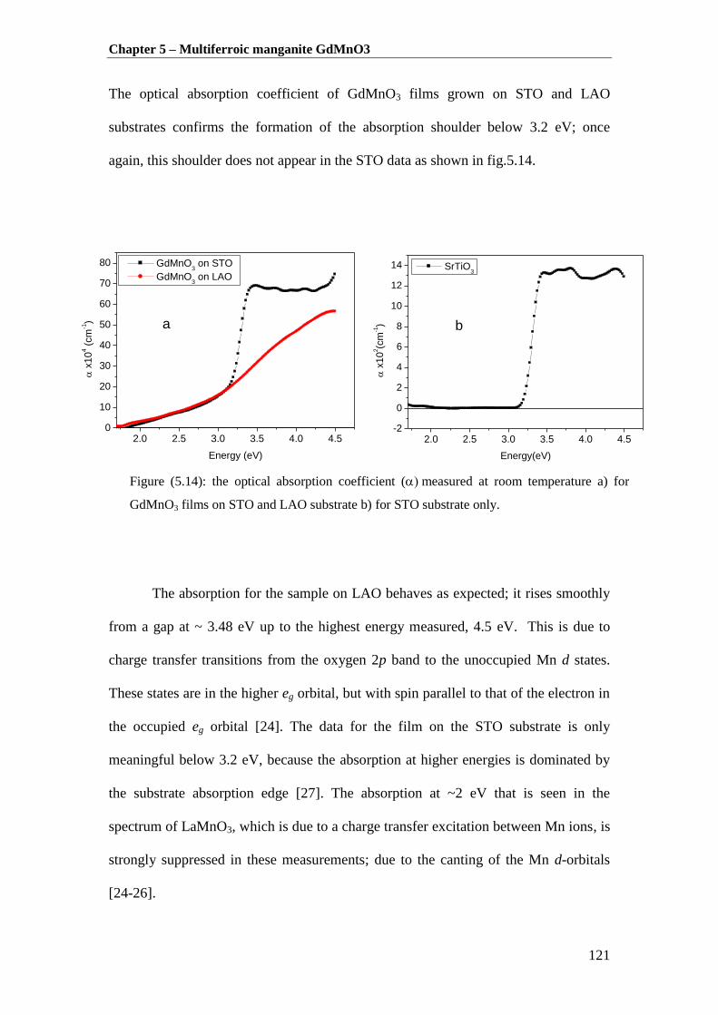
Chapter 5 – Multiferroic manganite GdMnO3
121
The optical absorption coefficient of GdMnO3 films grown on STO and LAO
substrates confirms the formation of the absorption shoulder below 3.2 eV; once
again, this shoulder does not appear in the STO data as shown in fig.5.14.
The absorption for the sample on LAO behaves as expected; it rises smoothly
from a gap at ~ 3.48 eV up to the highest energy measured, 4.5 eV. This is due to
charge transfer transitions from the oxygen 2p band to the unoccupied Mn d states.
These states are in the higher eg orbital, but with spin parallel to that of the electron in
the occupied eg orbital [24]. The data for the film on the STO substrate is only
meaningful below 3.2 eV, because the absorption at higher energies is dominated by
the substrate absorption edge [27]. The absorption at ~2 eV that is seen in the
spectrum of LaMnO3, which is due to a charge transfer excitation between Mn ions, is
strongly suppressed in these measurements; due to the canting of the Mn d-orbitals
[24-26].
Figure (5.14): the optical absorption coefficient (measured at room temperature a) for
GdMnO3 films on STO and LAO substrate b) for STO substrate only.
2.0 2.5 3.0 3.5 4.0 4.5-2
0
2
4
6
8
10
12
14
b
x
10
2(c
m-1)
Energy(eV)
SrTiO3
2.0 2.5 3.0 3.5 4.0 4.50
10
20
30
40
50
60
70
80
a
GdMnO3 on STO
GdMnO3 on LAO
x
10
4 (
cm
-1)
Energy (eV)

Chapter 5 – Multiferroic manganite GdMnO3
122
The magneto-optics, MCD, spectra were measured in Faraday geometry, where the
magnetic field is applied normal to the plane of the film, i.e. along the c-axis. The
MCD spectra of the GdMnO3 on the LAO substrate exhibit a birefringence. Hence ,if
light passes through a crystal in the z direction and there are different fast and slow
directions in the x-y plane with two refractive indices n+n and n-n, then the MCD
spectra will exhibit oscillations in intensity. The MCD spectrum for this film was
measured in a field and in zero field at different orientations in order to avoid the
birefringence. However, it seems that the birefringence arises entirely from the
substrate and dominates the spectra measured in MCD geometry and there is no way
to avoid it, see fig.5.15. Therefore, it does not seem possible to look for the strain
effects related to the ferroelectricity in this film.
The STO substrate undergoes a structural transition at about 100 K which
gives rise to the birefringence, unless the E vector of the light is along one of the optic
axes [28]. The samples were oriented carefully so this effect was not a perturbing
Figure (5.15): Ellipticity spectra measured at room temperature for a GdMnO3 film on
LAO substrate measured a) in a magnetic field, b) in zero field. These show the
importance of birefringence in LAO on these measurements.
1.5 2.0 2.5 3.0 3.5-5
-4
-3
-2
-1
0
1
2
3
4
5
b
Elli
pticity (
arb
.units)
Energy(eV)
0 degree
45 degree
70 degree
90 degree
1.5 2.0 2.5 3.0 3.5
-1.5
-1.0
-0.5
0.0
0.5
1.0
1.5 a
Elli
pticity (
arb
i.u
nits)
Energy(eV)
0 degree
45 degree
70 degree
90 dergee

Chapter 5 – Multiferroic manganite GdMnO3
123
feature. The temperature dependence of the MCD obtained from a blank substrate was
measured and these spectra were subtracted from the spectra of the film on the
substrate in order to obtain just the contribution from the film. Fig.5.16 shows the
MCD spectrum as a function of temperature for the GdMnO3 films grown on STO in
fields up to 0.5 T. This measurement was undertaken with the help of Alshammari in
the University of Sheffield. The plot shows two main spectral features a positive
feature at 2 eV and a negative feature at about 3 eV. In GdMnO3 the shape of the
MCD spectrum near 2 eV follows the expected absorption because the allowed
transitions are dominated by the spin occupations of the Mn d orbitals. Transitions to
unoccupied d levels with opposite spin are higher in energy by the Hubbard energy,
JH ~1 eV, and so would appear at different parts of the spectrum.
Figure (5.16): Temperature dependence of the MCD of GdMnO3 measured at 0.5 T. The
contribution from a blank STO substrate has been subtracted from this data.
1.6 1.8 2.0 2.2 2.4 2.6 2.8 3.0-40
-30
-20
-10
0
10
20
30
MC
D (
10
3 D
egre
e/c
m)
Energy(eV)
5K
10K
20K
30K
40K
50K
60K
70K
80K
90K
100K
200K
300K
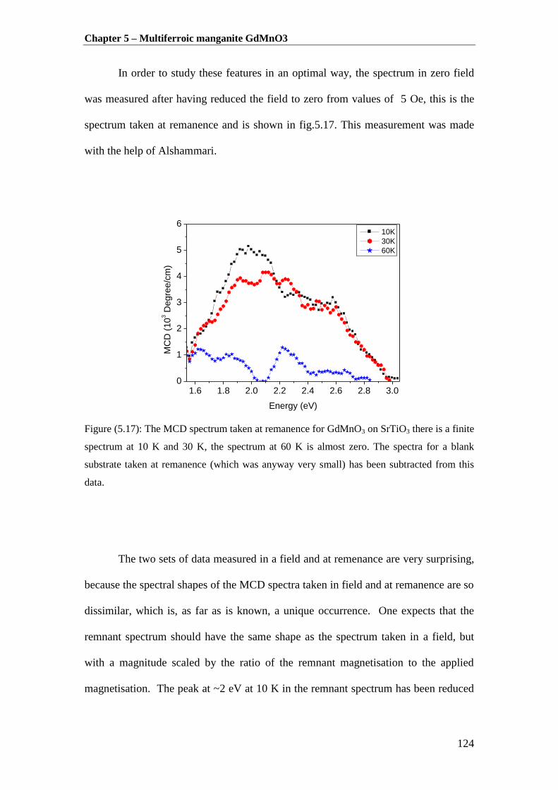
Chapter 5 – Multiferroic manganite GdMnO3
124
In order to study these features in an optimal way, the spectrum in zero field
was measured after having reduced the field to zero from values of 5 Oe, this is the
spectrum taken at remanence and is shown in fig.5.17. This measurement was made
with the help of Alshammari.
Figure (5.17): The MCD spectrum taken at remanence for GdMnO3 on SrTiO3 there is a finite
spectrum at 10 K and 30 K, the spectrum at 60 K is almost zero. The spectra for a blank
substrate taken at remanence (which was anyway very small) has been subtracted from this
data.
The two sets of data measured in a field and at remenance are very surprising,
because the spectral shapes of the MCD spectra taken in field and at remanence are so
dissimilar, which is, as far as is known, a unique occurrence. One expects that the
remnant spectrum should have the same shape as the spectrum taken in a field, but
with a magnitude scaled by the ratio of the remnant magnetisation to the applied
magnetisation. The peak at ~2 eV at 10 K in the remnant spectrum has been reduced
1.6 1.8 2.0 2.2 2.4 2.6 2.8 3.00
1
2
3
4
5
6
MC
D (
10
3 D
egre
e/c
m)
Energy (eV)
10K
30K
60K

Chapter 5 – Multiferroic manganite GdMnO3
125
by a factor of ~5 relative to its value in field; this is comparable to the ratio of Mr/Ms
observable in the SQUID data shown in fig.5.8.
These spectra can be understood when it is realised that the two optical
features at 3 eV and the 2 eV peak give two distinct components of the MCD spectra
with different temperature and field dependencies.
The negative feature occurring at 3 eV and it changes only slightly between
5 K and 40 K, in spite of the fact that the susceptibility is rising strongly over this
temperature range; also, a finite MCD signal is visible out to high temperatures. This
feature vanishes when the magnetic field is zero. Moreover, close to the structural
transition of STO at ~100 K it was also found to exhibit a large, strongly temperature
dependent, circular dichroism just below its band gap that varied linearly with the
applied magnetic field as will be discussed later in chapter 6. This signal was
considerably larger than the MCD of the film, because the thickness of the substrate,
0.5mm, was so much larger than that of the film ~100 nm; since it had a strong
temperature dependence, it was very hard to subtract the substrate data from the data
taken with the film. Since the substrate dichroism was purely paramagnetic, it did not
contribute to the remnant spectrum shown in fig.5.17. The MCD peak at 3 eV shown
in fig.5.15 is, therefore, due to the remaining contribution from the STO Substrate.
The energy of the transition at about 2 eV is characteristic of the charge
transfer transition between neighbouring Mn ions and depends on the overlap of the
spin states such that for adjacent spins oriented at an angle to each other this
varies as [25, 29]. This could not be detected in the optical absorption data
shown in Fig. 5.13. The strength of this peak in the MCD spectrum as shown in
Fig.5.16 decreases much more rapidly with temperature, than the strength of the peak
at 3 eV. For example, there is a significant drop in the intensity of the 2 eV peak at

Chapter 5 – Multiferroic manganite GdMnO3
126
30 K relative to 5 K and it has been suppressed almost to zero at 60 K, whereas the
intensity of the 3 eV peak at 30 K is changed very little compared with the data taken
at 5 K and the intensity at 60 K has only dropped by a factor of ~2. This is consistent
with the strength of the 2 eV peak depending on the relative spin directions of two
neighbouring Mn ions, as it increases below the transition to the canted A-phase,
where the spins in the a-b planes are parallel. On the other hand, it is this peak that
survives in the remanence spectrum. One would expect a finite remnant spectrum
only when there is magnetic hysteresis, which should occur below the transition to the
canted phase at 18 K, and so it is very surprising to obtain such a high remanence
spectrum at 30 K. It is possible that the strain in the film is inducing a canted phase
already at TN. The peak in LaMnO3 that was suppressed at ~2 eV is, in fact, 3 peaks
at 1.9 eV, 2.3 eV and 2.6 eV and there are features in the remanence spectra that
might correspond to these peaks; this, however, is not certain. It is clear that the 2 eV
peak can be studied much better using MCD at remanence than in any other mode,
because other features are absent.
Figure (5.18): MCD and Faraday hysteresis loops obtained from magneto-optics
measurements (in arbitrary units) at 3 eV and 10 K.
-6 -4 -2 0 2 4 6-0.09
-0.06
-0.03
0.00
0.03
0.06
0.09
3eV
MCD
Rotation
Magnetic field (kOe)
MC
D
-0.6
-0.3
0.0
0.3
0.6
Ro
tatio
n

Chapter 5 – Multiferroic manganite GdMnO3
127
In order to understand the MCD spectra, hysteresis loops were measured using
MCD and Faraday rotation at different energies. It should be noted that the substrate
contributes to the loop signals. Fig.5.18 shows the loop obtained at 10 K and at 3 eV
as measured by Alshammari. The MCD loop was strongly energy-dependent, as
expected from the MCD spectra; the loop obtained with Faraday rotation is very
weakly dependent on energy, therefore, it is shown only at 3 eV; it is also more
influenced by the contribution from the substrate. The loop at 3 eV has a very small
remanence, as expected from the data in Fig.5.16 and the coercive field of ~10 Oe
seen in this hysteresis loop was anomalously low, compared with the value of 120 Oe
seen in the SQUID data at 10 K. However, this may be due to the small coercivity of
the substrate. The MCD and Faraday hysteresis loops at 3 eV confirm a large
paramagnetic response below the STO band gap. So that the optical and magneto-
optical properties of STO substrate is studied in detail as shown in chapter 6.

Chapter 5 – Multiferroic manganite GdMnO3
128
5.4 Summary and Conclusions
This chapter reported on the investigation of the magnetic, optical and
magneto-optical properties of epitaxial films of GdMnO3 grown on STO and LAO
substrate. Epitaxial films of GdMnO3 were grown on SrTiO3 and LaAlO3 substrates
using sputtering technique. The LaAlO3 was twinned and so produced a highly
strained film whereas the strain was less for the film grown on SrTiO3. There is a
structural transition in SrTiO3 at ~100 K [28, 30] and this may be straining the film
grown on this substrate at low temperatures. The Néel temperature is reduced and
there is some evidence that a canted phase appears with the onset of anti-
ferromagnetism.
The two well-known features in the optical spectrum [24-25], the charge
transfer transition between Mn d states at ~2 eV and the band edge transition from the
oxygen p band to the d states at ~3 eV are observed in the magnetic circular dichroism
(MCD); however they behaved very differently both as a function of magnetic field
and temperature. The optical absorption at 3 eV is much stronger than that at 2 eV
however the MCD is considerably stronger at 2 eV. The MCD at ~2 eV correlates
well with the Mn spin ordering and it is very notable that the same structure appears
on this spectrum as is seen in LaMnO3 [25]. The result shows that the MCD peak at
3 eV is dominated by the optical and birefringence properties of the SrTiO3 substrate
and the absorption of SrTiO3 substrate above its band gap at about 3.27 eV was
actually a limiting feature in this study. Over all, it would have been very difficult to
understand the MCD in field without also having the spectrum taken at remanence
which underlines the importance of this type of measurement.

Chapter 5 – Multiferroic manganite GdMnO3
129
5.5 References
1. T. Kimura, G. Lawes, T. Goto, Y. Tokura and A. P. Ramirez, Phys. Rev. B 71
(22) (2005).
2. H. Béa and et al., Journal of Physics: Condensed Matter 20 (43), 434221
(2008).
3. L. W. Martin and et al., Journal of Physics: Condensed Matter 20 (43), 434220
(2008).
4. G. Rogez, N. Viart and M. Drillon, Angew. Chem.-Int. Edit. 49 (11), 1921-
1923 (2010).
5. M. Gajek, M. Bibes, S. Fusil, K. Bouzehouane, J. Fontcuberta, A. Barthelemy
and A. Fert, Nat Mater 6 (4), 296-302 (2007).
6. R. Ramesh and N. A. Spaldin, Nat Mater 6 (1), 21-29 (2007).
7. D. I. Khomskii, J. Magn. Magn. Mater. 306 (1), 1-8 (2006).
8. J. Baier, D. Meier, K. Berggold, J. Hemberger, A. Balbashov, J. A. Mydosh
and T. Lorenz, Phys. Rev. B 73 (10), 100402 (2006).
9. C. Renu, N. R. Mala, S. L. Chaplot, N. K. Gaur and R. K. Singh, New Journal
of Physics 11 (7), 073041 (2009).
10. D. Lee, J. H. Lee, P. Murugavel, S. Y. Jang, T. W. Noh, Y. Jo, M. H. Jung, Y.
D. Ko and J. S. Chung, Appl. Phys. Lett. 90 (18) (2007).
11. J. H. Lee, P. Murugavel, D. Lee, T. W. Noh, Y. Jo, M. H. Jung, K. H. Jang
and J. G. Park, Appl. Phys. Lett. 90 (1), 012903-012903 (2007).
12. J. H. Lee, P. Murugavel, H. Ryu, D. Lee, J. Y. Jo, J. W. Kim, H. J. Kim, K. H.
Kim, Y. Jo, M. H. Jung, Y. H. Oh, Y. W. Kim, J. G. Yoon, J. S. Chung and T.
W. Noh, Advanced Materials 18 (23), 3125-3129 (2006).

Chapter 5 – Multiferroic manganite GdMnO3
130
13. B. Lorenz, A. P. Litvinchuk, M. M. Gospodinov and C. W. Chu, Physical
Review Letters 92 (8), 087204 (2004).
14. T. Lottermoser, T. Lonkai, U. Amann, D. Hohlwein, J. Ihringer and M. Fiebig,
Nature 430 (6999), 541-544 (2004).
15. M. Fiebig, T. Lottermoser, D. Frohlich, A. V. Goltsev and R. V. Pisarev,
Nature 419 (6909), 818-820 (2002).
16. T. Goto, T. Kimura, G. Lawes, A. P. Ramirez and Y. Tokura, Physical Review
Letters 92 (25), 257201 (2004).
17. T. Kimura, T. Goto, H. Shintani, K. Ishizaka, T. Arima and Y. Tokura, Nature
426 (6962), 55-58 (2003).
18. T. Kimura, S. Ishihara, H. Shintani, T. Arima, K. T. Takahashi, K. Ishizaka
and Y. Tokura, Phys. Rev. B 68 (6), 060403 (2003).
19. B. H. Kim and B. I. Min, Phys. Rev. B 80 (6), 064416 (2009).
20. J. Hemberger, S. Lobina, H. A. Krug von Nidda, N. Tristan, V. Y. Ivanov, A.
A. Mukhin, A. M. Balbashov and A. Loidl, Phys. Rev. B 70 (2), 024414
(2004).
21. K. Noda, S. Nakamura, J. Nagayama and H. Kuwahara, Journal of Applied
Physics 97 (10), 10C103-103 (2005).
22. J. Baier, D. Meier, K. Berggold, J. Hemberger, A. Balbashov, J. A. Mydosh
and T. Lorenz, J. Magn. Magn. Mater. 310 (2, Part 2), 1165-1167 (2007).
23. X. L. Wang, J. Appl. Phys. 107 (9), 09B510 (2010).
24. M. W. Kim and et al., New Journal of Physics 6 (1), 156 (2004).
25. M. W. Kim, S. J. Moon, J. H. Jung, J. Yu, S. Parashar, P. Murugavel, J. H.
Lee and T. W. Noh, Physical Review Letters 96 (24), 247205 (2006).
Chapter 5 – Multiferroic manganite GdMnO3
131
26. M. Bastjan, S. G. Singer, G. Neuber, S. Eller, N. Aliouane, D. N. Argyriou, S.
L. Cooper and M. Rübhausen, Phys. Rev. B 77 (19), 193105 (2008).
27. K. van Benthem, J. Appl. Phys. 90 (12), 6156 (2001).
28. M. A. Geday and A. M. Glazer, Journal of Physics: Condensed Matter 16 (20),
3303 (2004).
29. A. M. Haghiri-Gosnet and J. P. Renard, Journal of Physics D: Applied Physics
36 (8), R127 (2003).
30. D. Pesquera, V. Skumryev, F. Sánchez, G. Herranz and J. Fontcuberta, Phys.
Rev. B 84 (18), 184412 (2011).

Chapter 6 - Strontium Titanate STO Substrates
132
Chapter 6
Strontium Titanate STO Substrates
6.1 Introduction
STO was the substrate chosen for growing LSMO and GdMnO3 films as it
was expected to be a low-strain substrate. However, the films grown on substrates of
this material showed anomalous magneto-optical behaviour as was discussed in
chapters 4 and 5. The present chapter will provide an investigation of the optical and
magneto-optical properties of a STO substrate in order to understand the earlier result.
The influence of birefringence on the magneto-optical data obtained using the Sato
method is discussed.
6.2 Literature on Optical and Magneto-Optical Properties of STO
Substrates
A large number of materials have great potential for possible industrial
applications. These applications require that the material be grown in thin-film form
rather than in the bulk. In recent years, many research groups have studied the
difference between the properties of thin films and bulk materials. The thin films have
been grown to optimise the structural and physical properties. It is found that some
properties, such as structural deformation and magnetic/optical anisotropy, are
strongly dependent on the nature of the substrate [1-5]. Such results could often be
attributed to the stress induced by the lattice mismatch between film and substrate [3,
5]. In particular, a cubic substrate, such as STO, commonly induces either a
compressive or a tensile bi-axial strain on the growing film [6]. STO is probably the

Chapter 6 - Strontium Titanate STO Substrates
133
most commonly used substrate for growing epitaxial thin manganites films, as it is
one of the more important oxide materials for potential device applications [6-7].
However, STO substrates display birefringence which, in turn, has an effect on the
optical and magneto-optical properties. The ray of light that passes through a
birefringent material is split into two unequal waves which propagate with different
speeds. Thus, birefringent crystals have a refractive index that depends on the
polarisation and propagation direction of the incident light; clearly then, it is not the
same at all angles.
STO has the ABO3 cubic perovskite structure with a lattice parameter of
0.3905 nm. In addition, STO substrates can be used at a high deposition temperature
due to their high melting point of around 2080 [8]. In the perovskite structure, there
are always two types of terminating planes. For instance, STO (001) has A (SrO) or B
(TiO2) terminating planes in the directions see fig.6.1 where, the topmost
surface of the STO is terminated by either one of these planes.
Removed by the
author for copyright reasons
Figure (6.1): The ABO3 cubic perovskite crystal structure of STO and possible terminating
planes of a { } surface [8].

Chapter 6 - Strontium Titanate STO Substrates
134
At room temperature, STO has a cubic perovskite structure but undergoes a
phase transition to a tetragonal structure at about 105 K [6]. The TiO6 octahedra
rotate around the cubic axis, whereas the oxygen ions remain in its position in the face
of the unit cell. This leads to an expansion in the c- axis direction and a contraction in
the a-axis direction, which results in a tetragonal structure. This transition leads to
birefringence in the STO substrate, unless the E vector of the light is directed along
one of the optic axes [6, 9].
Removed by the
author for copyright reasons
Figure (6.2): Birefringence in STO as a function of temperature. The straight line is a fit to
the observed data [9].

Chapter 6 - Strontium Titanate STO Substrates
135
It was found that the birefringence n) is directly proportional to the
temperature [9] below the phase transition temperature, as illustrated in fig.6.2. The
birefringence increased as the temperature decreased below a critical value 105K,
which is the phase transition of the STO substrate.
The properties of STO can easily be changed by doping or by introducing
oxygen vacancies. Hence, STO can be made n-type conducting by doping with a
small fraction of La, Nb or Ta [10]. However, oxygen vacancies can be introduced
into STO substrates during film deposition, which may have an effect on the
properties of the film.
STO is a dielectric material with a band gap at about 3.2 eV at 300 K [10-11].
Studies of the optical properties of STO found that the absorption near the band edge
was attributed to phonon-assisted indirect transition. Blazey [12] measured the
wavelength-modulated absorption spectrum of STO around the structural phase
transition for various temperatures; this is shown in fig. 6.3. There is a single
minimum at all temperatures above and below the phase transition 105 K; this was
thought to be due to an indirect transition, as it is not seen in the modulated reflection
spectrum.
Zollner et al studied the optical properties of bulk STO with a thickness of 0.5
mm. They measured the absorption coefficient and the band gap was found to be
about 3.25 to 3.37 eV [13], as illustrated in fig. 6.4. This is similar to what had
previously been measured, as is shown in chapter 5 fig. 5.14.

Chapter 6 - Strontium Titanate STO Substrates
136
Removed by the
author for copyright reasons
Figure (6.3): The wavelength-modulated absorption spectrum of STO at various temperatures
around the structural phase transition [12].
Removed by the
author for copyright reasons
Figure (6.4): The optical absorption coefficient (α) as a function of photon energy for bulk
STO. The inset is √ in the region of the indirect band gap (3.2 eV). This figure was taken
from [13].

Chapter 6 - Strontium Titanate STO Substrates
137
6.3 Experiment Results and Discussion
In order to study the optical and magneto-optical properties of STO substrates,
a (001) sample of dimensions 5mm 5mm 0.5 mm was employed. The STO (001)
substrate which was polished on both sides was purchased from PyKem.
The optical properties were measured at room temperature in the spectral
range 1.5-4.5 eV using the absorption system. The magneto- optical properties were
measured in the same range using Faraday geometry in applied magnetic fields up to
1.8 Tesla perpendicular to surface of the samples. The substrate was rotated with ( )
varying from 0º to 360º relative to the polarisation of the analyser, as shown in fig.6.5.
𝜓
Polarisation axis of
the analyser (x) Optical axis of
STO substrate
Linearly Polarised
light
x
Z
Y
STO substrate
Figure 6.5: Sketch showing the set-up used for studying the magneto-optical properties
of an STO substrate in Faraday geometry.

Chapter 6 - Strontium Titanate STO Substrates
138
2.0 2.5 3.0 3.5 4.0 4.5 5.0
-6
-4
-2
0
dT
/dE
Energy (eV)
SrTiO3 (STO)
The transmission of STO has previously been measured; it has also been
mentioned that STO has an indirect band gap at 3.2 eV . This was shown in fig.5.11,
chapter 5. In order to study this more carefully, the derivative spectrum (dT/dE) was
calculated, as shown in fig. 6.6. The derivative spectrum removes the background and
amplifies the singularity. This shows that the lowest, indirect band gap for our STO
substrate occurs at 3.26 eV.
The magneto-optical set-up which is based upon Sato method [14] involves, a
measurement of three intensities I0, I1(f) and I2(2f) being transmitted through the
sample, as discussed in chapter 3. In the absence of any birefringence in the sample,
the intensity I1(f) is proportional to the MCD and I2(2f) is proportional to the Faraday
rotation (θ). However, in the presence of the birefringence, this contributes to both
Figure (6.6): The derivative spectrum (dT/dE) versus photon energy for an STO substrate in the
region of the band gap, measured at room temperature.
The

Chapter 6 - Strontium Titanate STO Substrates
139
I1(f) and I2(2f). With detailed and complex mathematics, the final intensities of I1(f)
and I2(2f), after passing through the Sato rig, are given by:
(
) [ ]
…………..6.1
(
) [ ]
…………..6.2
The derivation plus further details are given in Appendix A. The term is
the true ellipticity, is the rotation, is the ellipticity and is the sense of
rotation; is the only parameter that changes sign with magnetic field. The
measurement can be taken both in magnetic field (H) and in zero field. In the case of
measurements made in a field, the difference between the measurements for +H and –
H is taken and only terms in remain:
(
) 6.3
[ ] [ ] 6.4
From equations (6.3) and (6.4) there is a term varying like the
squared in
the
unless
. The aim is to eliminate this term in order to find
, where
is the true
signal.
The spectra of I1(f)/I0 and I2(2f)/I0 for the STO substrate were measured in-
field at different orientations ( ) of the STO substrate relative to the polarisation of

Chapter 6 - Strontium Titanate STO Substrates
140
the analyser. Fig.6.7 shows the I1(f)/I0 spectrum of the STO substrate at different
orientations, measured at room temperature in a field of 1.8 T. The data shows two
features: one at the band edge and a negative feature at the lower energy. This
indicates that, below the band gap, the I1(f)/I0 spectrum varied with the applied
magnetic field and is orientation dependent. The dependence of I1(f)/I0 on orientation
appears to be due to the magnetically induced birefringence in the substrate. Now we
need to find the orientation of the substrate which gives the lowest birefringence.
The magnitude of I1(f)/I0 and I2(2f)/I0 were plotted as a function of orientation,
as shown in fig. 6.8 and fig.6.9. The data indicates that the birefringence in the
substrate was enhanced by a magnetic field, which is surprising and unexpected.
Moreover, the data is reproducible and non-periodic as expected. The relation
between the birefringence (Δ) and the orientation angle ( ) are given as:
√
√
6.4
The derivation and further details are given in Appendix A. The magnetism is
included in the term . If
or when the birefringence dominated we found:
6.5
I1(f)/I0 is proportional to or . This vanishes ( if or are
such that:
…….

Chapter 6 - Strontium Titanate STO Substrates
141
However, the data shown in fig.6.8 did not exhibit a periodic variation with 180º,
which is surprising. By looking to the case at when the birefringence (Δ) is zero, and
from equation 6.4 it is found that:
=1 and
6.6
Figure (6.7): Room temperature I1(f)/I0 spectra for STO substrate at different
orientation measured in 1.8 T.
1.6 1.8 2.0 2.2 2.4 2.6 2.8 3.0 3.2 3.4
-0.1
0.0
0.1
0.2
0.3
34
5
6
7
891011
1213
1415
1617
18192021
22232425
26272829303132333435363738394041424344454647484950515253545556575859606162636465666768697071727374757677787980818283848586878889909192
CD
E
F
G
H
I
JKLMN
OP
QR
ST
UV
WX
YZAAABACADAEAFAGAHAIAJAKALAMANAOAPAQARASATAUAVAWAXAYAZBABBBCBDBEBFBGBHBIBJBKBLBMBNBOBPBQBRBSBTBUBVBWBXBYBZCACBCCCDCECFCGCHCICJCKCLCMCNCO
cd
e
f
g
hijklm
no
pq
rst
uv
wxy
zaaabacadaeafagahaiajakalamanaoapaqarasatauavawaxayazbabbbcbdbebfbgbhbibjbkblbmbnbobpbqbrbsbtbubvbwbxbybzcacbcccdcecfcgchcicjckclcm
cn
3
45
67
8
91011121314
1516
1718
19202122
232425262728293031323334353637383940414243444546474849505152535455565758596061626364656667686970717273
7475767778
798081828384858687888990919293
STO substrate
I 1/I
0 (
arb
.un
its)
Energy (eV)
0
10
20
30
40
50
60
70
80
90
100
110
120
130
140
1501 160A 170a 180
190
200
210
220
230
240
250
260
270
280
290
300
310
320
330
3401 350

Chapter 6 - Strontium Titanate STO Substrates
142
Figure (6.8): I1(f)/I0 values at room temperature taken around the band edge versus
the orientation of an STO substrate. The data was measured in 1.8 T.
Figure (6.9): I2(2f)/I0 values at room temperature taken at different photon energy
versus the orientation of STO substrate. The data was measured in 1.8 T.
0 50 100 150 200 250 300 350 400
-0.10
-0.05
0.00
0.05
0.10
0.15
0.20
0.25
0.30 peak magnitude
In field
300KI 1
/I0(a
rb.u
nits)
Orientation (degree)
-50 0 50 100 150 200 250 300 350 400
2.9
3.0
3.1
3.2
3.3
3.4
3.5
I 2/I
0(
arb
.units)
Orientation (degree)
3.14 eV
3.16 eV
3.18 eV
3.2 eV
3.22 ev
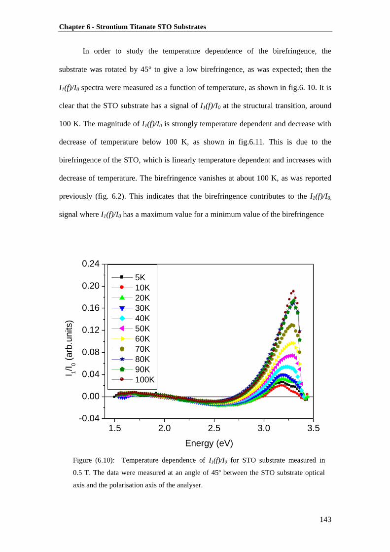
Chapter 6 - Strontium Titanate STO Substrates
143
In order to study the temperature dependence of the birefringence, the
substrate was rotated by 45 to give a low birefringence, as was expected; then the
I1(f)/I0 spectra were measured as a function of temperature, as shown in fig.6. 10. It is
clear that the STO substrate has a signal of I1(f)/I0 at the structural transition, around
100 K. The magnitude of I1(f)/I0 is strongly temperature dependent and decrease with
decrease of temperature below 100 K, as shown in fig.6.11. This is due to the
birefringence of the STO, which is linearly temperature dependent and increases with
decrease of temperature. The birefringence vanishes at about 100 K, as was reported
previously (fig. 6.2). This indicates that the birefringence contributes to the I1(f)/I0,
signal where I1(f)/I0 has a maximum value for a minimum value of the birefringence
Figure (6.10): Temperature dependence of I1(f)/I0 for STO substrate measured in
0.5 T. The data were measured at an angle of 45º between the STO substrate optical
axis and the polarisation axis of the analyser.
1.5 2.0 2.5 3.0 3.5-0.04
0.00
0.04
0.08
0.12
0.16
0.20
0.24
I 1/I
0 (
arb
.units)
Energy (eV)
5K
10K
20K
30K
40K
50K
60K
70K
80K
90K
100K

Chapter 6 - Strontium Titanate STO Substrates
144
It is clear from fig.6.11 that, below the phase transition temperature (100 K) of
the STO, the I1(f)/I0 signal is temperature dependent. However, the birefringence is
also temperature dependent and decreased linearly as the temperature was increased.
This indicates that the birefringence has a strongly influence on the I1(f)/I0 data and
dominates below the temperature of the phase transition. The birefringence values
were expected to vary with temperature as follows:
6.7
Figure (6.11): Magnitude of I1(f)/I0 for SrTiO3 (STO) substrate as a function of
temperature taken at 0.5 T. The data was measured at 45º between the STO substrate
optical axis and the polarisation axis of the analyser.
0 20 40 60 80 1000.00
0.04
0.08
0.12
0.16
0.20I 1
/I0 (
arb
.units)
Temperature (K)
STO data at 45 degree
to the polarization axis
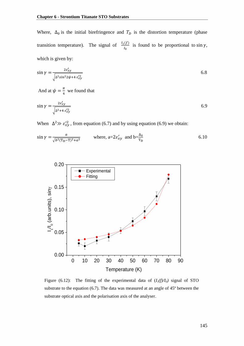
Chapter 6 - Strontium Titanate STO Substrates
145
Where, is the initial birefringence and is the distortion temperature (phase
transition temperature). The signal of
is found to be proportional to ,
which is given by:
√
6.8
And at
we found that
√
6.9
When , from equation (6.7) and by using equation (6.9) we obtain:
√ where, a=
and b=
6.10
Figure (6.12): The fitting of the experimental data of (I1(f)/I0) signal of STO
substrate to the equation (6.7). The data was measured at an angle of 45º between the
substrate optical axis and the polarisation axis of the analyser.
0 10 20 30 40 50 60 70 80 900.00
0.05
0.10
0.15
0.20
I 1/I
0 (
arb
.units),
sin
Temperature (K)
Experimental
Fitting
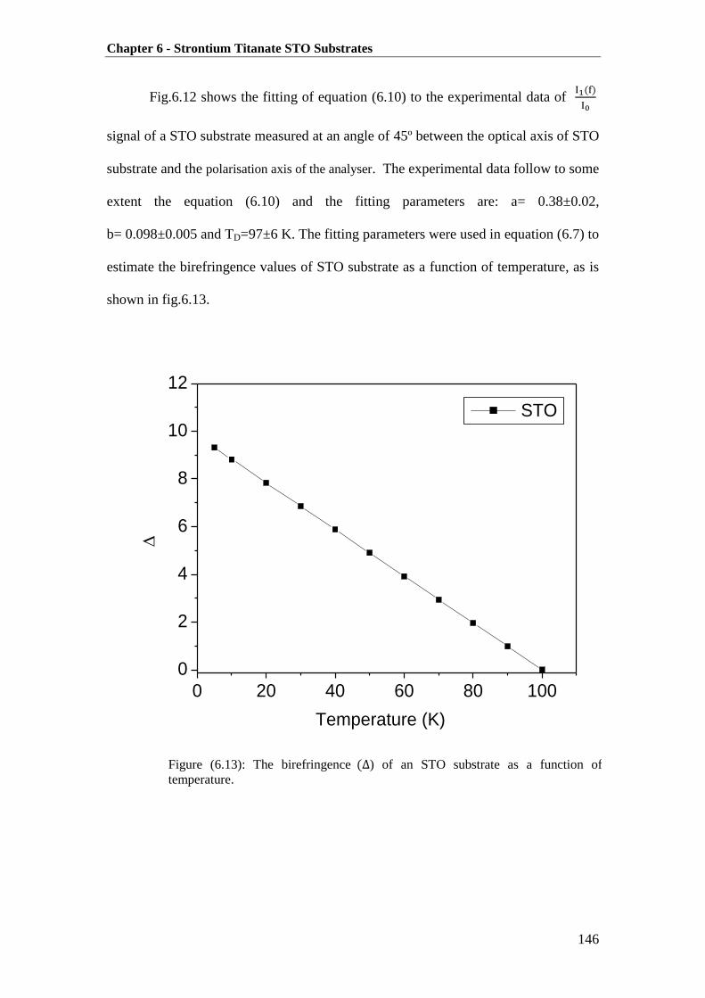
Chapter 6 - Strontium Titanate STO Substrates
146
Fig.6.12 shows the fitting of equation (6.10) to the experimental data of
signal of a STO substrate measured at an angle of 45º between the optical axis of STO
substrate and the polarisation axis of the analyser. The experimental data follow to some
extent the equation (6.10) and the fitting parameters are: a= 0.38±0.02,
b= 0.098±0.005 and TD=97±6 K. The fitting parameters were used in equation (6.7) to
estimate the birefringence values of STO substrate as a function of temperature, as is
shown in fig.6.13.
0 20 40 60 80 100
0
2
4
6
8
10
12
Temperature (K)
STO
Figure (6.13): The birefringence ) of an STO substrate as a function of
temperature.

Chapter 6 - Strontium Titanate STO Substrates
147
In the case of measurements taken in zero field; there is no correction for +H
and –H and and . Thus, the
and
signals should be
interchanged and given as:
6.11
6.12
Fig. 6.14 and 6.15 show the spectra measured in zero field for I1(f)/I0 and
I2(2f) /I0 respectively. This result shows that the spectrum depended on angle for both
I1(f) /I0 and I2(2f) /I0. This result is evidence for a birefringent contribution from the
STO substrate in zero field. However these data do not agree with the expected results
from equations 6.11 and 6.112.
Finally, we can conclude that the birefringence in the STO substrate is both
field and temperature dependent, which makes the behaviour of the birefringence very
complicated.

Chapter 6 - Strontium Titanate STO Substrates
148
Figure (6.14): Room temperature I1(f)/I0 spectra for STO substrate at different orientations
and measured in zero field.
.
Figure (6.15): Room temperature I2(2f) /I0 spectra for STO substrate at different orientations and
measured in zero field.
1.5 2.0 2.5 3.0 3.5-0.20
-0.16
-0.12
-0.08
-0.04
0.00
0.04
0.08
0.12
I 1(f
)/I 0
(a
rb.u
nits)
Energy (eV)
0 Deg
22.5
45
67.5
90
1.5 2.0 2.5 3.0 3.5
-0.05
0.00
0.05
0.10
0.15
0.20
0.25
0.30
0.35
I 2(2
f)/I
0 (
arb
.units)
Energy (eV)
0 Deg
22.5
45
67.5
90
Chapter 6 - Strontium Titanate STO Substrates
149
6.4 Summary and Conclusions
This chapter reported the investigation of the derivative spectrum and the
magneto-optical properties of an STO substrate. We have also discussed the influence
of birefringence on the magneto-optics of the substrate obtained using the Sato
method.
The derivative spectrum data shows that the lowest indirect band gap for the
STO substrate occurs at 3.26 eV. The MCD peak appears at a slightly lower value
than that seen in the energy modulated experiment; this could be due to the different
thicknesses. The data indicated that the substrate has circular dichroism (MCD) below
the band gap, which is strongly temperature dependent and varies linearly with
applied magnetic field. The data indicates that the magnetic field enhanced the
birefringence in the STO substrate and the birefringence is both orientation and
temperature dependent.
Overall, STO substrate were used to grow LSMO and GdMnO3 thin films and
did have an anomalous magneto-optical data, as discussed in chapters 4 and 5. In
order to avoid the birefringence, the optical and magneto-optical properties of the
substrate were studied. It seems that the relation between the birefringence on the one
hand and the magnetic field, orientation and temperature on the other hand is very
complex. It is difficult to determine the value of the birefringence and correct the data
of the films grown on an STO substrate.
In summary, we do not recommend using STO substrate for the growth of
films for optical study for E .

Chapter 6 - Strontium Titanate STO Substrates
150
6.5 References
1. R. Desfeux, S. Bailleul, A. Da Costa, W. Prellier and A. M. Haghiri-Gosnet,
Applied Physics Letters 78 (23), 3681-3683 (2001).
2. A. M. Haghiri-Gosnet, J. Wolfman, B. Mercey, C. Simon, P. Lecoeur, M.
Korzenski, M. Hervieu, R. Desfeux and G. Baldinozzi, Journal of Applied
Physics 88 (7), 4257-4264 (2000).
3. C. Kwon, M. C. Robson, K. C. Kim, J. Y. Gu, S. E. Lofland, S. M. Bhagat, Z.
Trajanovic, M. Rajeswari, T. Venkatesan, A. R. Kratz, R. D. Gomez and R.
Ramesh, Journal of Magnetism and Magnetic Materials 172 (3), 229-236
(1997).
4. W. Prellier, M. Rajeswari, T. Venkatesan and R. L. Greene, Applied Physics
Letters 75 (10), 1446-1448 (1999).
5. J. Z. Sun, D. W. Abraham, R. A. Rao and C. B. Eom, Applied Physics Letters
74 (20), 3017-3019 (1999).
6. D. Pesquera, V. Skumryev, F. Sánchez, G. Herranz and J. Fontcuberta,
Physical Review B 84 (18), 184412 (2011).
7. C. H. Jia, Y. H. Chen, G. H. Liu, X. L. Liu, S. Y. Yang and Z. G. Wang,
Journal of Physics D: Applied Physics 42 (1), 015415 (2009).
8. G. Koster, G. Rijnders, D. H. A. Blank and H. Rogalla, Physica C:
Superconductivity 339 (4), 215-230 (2000).
9. M. A. Geday and A. M. Glazer, Journal of Physics: Condensed Matter 16 (20),
3303 (2004).
10. A. Kalabukhov, R. Gunnarsson, J. Börjesson, E. Olsson, T. Claeson and D.
Winkler, Physical Review B 75 (12), 121404 (2007).

Chapter 6 - Strontium Titanate STO Substrates
151
11. M. L. Scullin, J. Ravichandran, C. Yu, M. Huijben, J. Seidel, A. Majumdar
and R. Ramesh, Acta Materialia 58 (2), 457-463 (2010).
12. K. W. Blazey, Physical Review Letters 27 (3), 146-148 (1971).
13. S. Zollner, A. A. Demkov, R. Liu, P. L. Fejes, R. B. Gregory, P. Alluri, J. A.
Curless, Z. Yu, J. Ramdani, R. Droopad, T. E. Tiwald, J. N. Hilfiker and J. A.
Woollam, J. Vac. Sci. Technol. B 18 (4), 2242-2254 (2000).
14. K. Sato, Japanese Journal of Applied Physics 20 (12), 2403-2409 (1981).

Chapter 7 - Transition Metal (TM) Doped In2O3
152
Chapter 7
Transition Metal (TM) Doped In2O3
7.1 Introduction
Transition metal (TM)-doped semiconductor oxides are promising material to
show ferromagnetism above room temperature. This chapter reports an investigation
of the magnetic and magneto optical properties of Fe and Co doped indium Oxide
(In2O3). It also provides a simple method to determine the contribution from the TM
to the ferromagnetic moment of the films. The Co-doped In2O3 data presented in this
chapter was published in [1].
7.2 Literature Review on TM Doped In2O3
Many oxide semiconductors such as ZnO, SnO2, In2O3, and TiO2 doped with
transition metal TM have been reported to be a ferromagnetic FM beyond room
temperature [2, 4-11]. Recently, a number of research groups have conducted
thorough studies of high ferromagnetism FM in a number of TM doped-In2O3
systems. The room temperature ferromagnetism has been reported for all 3d TM such
as (V, Cr, Fe, Cu, Ni and Co) [3, 12-25]. In2O3 crystallizes in the cubic structure with
lattice constant about a=10.12 with 80 atoms or 16 formula units per unit cell [14].
This gives In2O3 an advantage as a host material because it can be grown on low cost
substrates such as MgO and Al2O3 [13, 26]. In2O3 is a wide band-gap semiconductor
(3.75 eV) and is transparent in the visible [4, 24, 27]. It can be prepared as an n-type
semiconductor with a high electrical conductivity by introducing oxygen deficiencies

Chapter 7 - Transition Metal (TM) Doped In2O3
153
or by Sn doping (ITO) [12, 14]. Sn-doped In2O3 with 10% produces transparent
n-type conducting semiconductor which can be widely used in device applications. It
is widely used in semiconductor devices such as optoelectronics and photovoltaics
[28-29]. This has shown a high carrier concentration at about 1020
- 1021
electrons/
cm3
with high mobility at about (10- 100) cm2
.V-1
.s-1
[16, 26, 30].
Recently, room temperature (RT) ferromagnetism has been reported for Co-
doped indium oxide (ITO) [31]. This ferromagnetism behaviour has found to be
correlated to the transport properties. Moreover, metallic Co clusters have been
observed in many cases of thin films but the high-temperature annealing remove these
nanoclusters [12, 31].
The origin of ferromagnetism remains unclear although the ferromagnetism
properties are strongly affected by many parameters such as growth, annealing
processes, defects and substrate nature [12, 16, 31]. However, the origin of the
ferromagnetism in TM doped oxides semiconductors was thought to be due the
interaction between the s and p band of the host and the localized 3d electrons in TM
band [1, 32], whereas, other researchers have reported that the TM ions are
paramagnetic [32-33]. Several groups have looked hard for evidence of ferromagnetic
behaviour using local probes, X-ray magnetic circular dichroism (XMCD) or
Mossbauer effect. A Brillion function has been fitted to the M(H) curves of Co doped
ZnO recorded from XMCD using a magnetic moment of 4.8 /Co which is related to
Co+2
[34-35]. The analysis of Mossbauer spectroscopy of Fe doped ITO showed a
paramagnetic pattern for Fe+2
and Fe+3
[2]. In all cases they have found that the TM
ions themselves have a magnetization that varies as H/T which means purely
paramagnetic behaviour of TM. Coey has analysed the susceptibility of a strongly
magnetic sample at low temperature and found for Mn in ITO that the susceptibility

Chapter 7 - Transition Metal (TM) Doped In2O3
154
varied as C/T where the Curie constant C was exactly what would be predicted for
Mn+2
[2] as illustrated in fig.7.1. Similar result was found for Co+2
doped ITO [32]
and Zn1-xCoxO [34-35]. Moreover, some research groups have reported that the films
of In2O3 with TM2+
are ferromagnetic whereas all those relating to solely TM3+
are
not ferromagnetic [36-37].On the other hand mixed valence of TM2+
/TM3+
is reported
to be origin of the magnetism [38] whereas there is good evidence that actually the
TM ions are not ferromagnetic.
Removed by the
author for copyright reasons
The recent research focuses on investigating the link between the defects and
the ferromagnetism (FM). Oxygen vacancies are believed to be a critical role to
explain the ferromagnetism in oxide semiconductors. It is strongly believed that the
existence of oxygen vacancies in TM doped In2O3 plays a critical role in enhancing
Figure (7.1): Magnetisation curves at different temperature for 5% Mn-doped ITO films.
The inset is the Curie-law behaviour [2].

Chapter 7 - Transition Metal (TM) Doped In2O3
155
the ferromagnetism. Xiao-Hong et.al reported the decrease of magnetisation with the
increase of oxygen pressure for Fe-doped In2O3 films as shown in fig. 7.2 [3].
Removed by the
author for copyright reasons
Fe-doped In2O3 has particularly acquired a significant amount of interest due
to the high solubility, up to 20%, of Fe in the In2O3 matrix; this makes it an effective
system for application in spintronic devices and also for studying the physics that
underpins DMSs. However, the growth method and processing conditions are crucial
for the magnetic properties of Fe-doped In2O3. Room temperature ferromagnetism has
been reported in Fe- doped In2O3 bulk and thin films [20, 23, 38]. Very recently, room
temperature ferromagnetism has been reported in Fe-doped In2O3 thin films and others
attributed the ferromagnetism to the spin-polarised carriers [11].
Figure (7.2): Room temperature magnetisation for (In0.98 Fe0.02)2O3 films grown at various
oxygen pressures. Adopted from ref. [3]. Inset is the variation in the MS as a function of
oxygen pressure.

Chapter 7 - Transition Metal (TM) Doped In2O3
156
Cobalt (Co) is one of the TMs that shows high magnetisation. Room
temperature ferromagnetism has been reported in Co doped In2O3 and indium-tin
oxide (ITO) [30, 39]. Others attributed the ferromagnetism to different contributions
from oxidized (Co2+
) and from metallic cobalt (Co0). It was found in indium-tin oxide
films the Co atoms substitute homogeneously the indium (In) sites with less than 7%
of Co [19].
As far as is known, there is no published research on magneto-optical
properties of TM-doped In2O3 except our papers [1, 4]. However, there are number of
magneto-optical studies on dilute magnetic oxide materials (DMO) such as ZnO.
These studies have provided very useful information about the spin polarisation in
conduction electrons [40-42].

Chapter 7 - Transition Metal (TM) Doped In2O3
157
7.3 Experiment Results and Discussion:
7.3.1 Co Doped In2O3
In order to study the magnetic and magneto-optical properties of Co-doped
In2O3, five thin films of (In1-x Cox)2 O3 with normal Co concentration of 1-5% were
grown by A. Hakimi in the laboratory of Cambridge University using dc magnetron
sputtering. The Co concentration were measured using an energy dispersive x-ray
spectroscopy (EDX) and the actual value were 1.6, 3.1, 4.7 .6.4 and 8.1 %. The films
thickness was 200 nm grown in a highly oxygen-deficient environment on (0001)
C-plane sapphire substrate at . The data presented in this section was published
in [1].
Fig.7.3 shows XRD patterns of Co-doped In2O3 films performed by A. Hakimi
in Cambridge University. XRD patterns shows a relatively sharp peak and no
detectable peak corresponds to the secondary phases of Co metal or Co oxides. This
indicates that the films are pure phases and have high crystalline quality. With an
increase of Co doping levels, the In2O3 (222) and (400) peaks was found to be shifted
toward higher values of . This is evidence that the Co2+
ions with smaller ionic
radius (0.74 ) substitute for In3+
with larger ionic radius (0.94 ) rather than forming
a defect phase. Fig.7.4 shows the near-edge EXAFS data for the (In 0.919 Co 0.081)2 O3
film compared with CoO and Co metal performed by S.M. Heald in Argonne National
laboratory, USA. The EXAFS spectra indicate that Co is predominately Co2+
.
However, the small peak at about 7710 eV could be attributed to a small amount of
Co metal.

Chapter 7 - Transition Metal (TM) Doped In2O3
158
Removed by the
author for copyright reasons
Removed by the
author for copyright reasons
Figure (7.3): XRD data for (In1-x Cox)2 O3 films demonstrate the shift in the peak position
upon Co doping. The inset is the steady decrease in the average lattice parameter as a
function of Co doping [1]
Figure (7.4): Normalized Co near-edge EXAFS spectra for the 8.1% Co-doped In2O3
thin film compared with CoO and Co metal [1].

Chapter 7 - Transition Metal (TM) Doped In2O3
159
Magnetic properties were investigated using the superconducting quantum
device (SQUID) magnetometer. Fig.7.5 shows the magnetisation raw data of
(In1-x Cox)2 O3 films measured under in-plane magnetic field up to 1 T and in the
temperature range of 5-300 K. This data displays clear evidence for ferromagnetism
in each of the Co-doped In2O3 films up to and above room temperature.
The raw magnetisation data was decomposed into two parts. The first varies
linearly with the magnetic field in the range of (0.5 -1 T) and the second is a
hysteresis loop as shown in fig.7.5. The paramagnetic susceptibility ( ) is worked out
from the slope of the linear part, then the curie constant Cmeas was calculated. Since
the susceptibility ( ) of the substrate is temperature independent and since the
paramagnetic susceptibility ( ) at 300 K is expected to be very small, we can estimate
the paramagnetic contribution of the films at 5 K from ( ) ( )
( ). The susceptibility ( ) at 5K for these films has been set as C/5 then
evaluated Curie constant (C) for the concentration of TM ions. The expected
-10000 -5000 0 5000 10000
-2.0x10⁻⁴
-1.0x10⁻⁴
0.0
1.0x10⁻⁴
2.0x10⁻⁴ 5K
Magnetic m
om
ent (e
mu)
Magnetic field (Oe)
8.1%
6.4%
4.7%
3.1%
1.6%
-10000 -5000 0 5000 10000
-3.0x10⁻⁴
-2.0x10⁻⁴
-1.0x10⁻⁴
0.0
1.0x10⁻⁴
2.0x10⁻⁴
3.0x10⁻⁴
300K 8.1%
6.4%
4.7%
3.1%
1.6%
Ma
gn
etic m
om
ent(
em
u)
Magnetic field (Oe)
Figure (7.5): The raw magnetisation data for (In1-x Cox)2 O3 thin films measured at a) 5K
b) 300K.

Chapter 7 - Transition Metal (TM) Doped In2O3
160
paramagnetic susceptibility ( ) from the TM ions was calculated using
where is the effective number of Bohr magnetons ( ), N is the
number of host ions per cm3 and is the TM concentration. Fig.7.6 represents the
susceptibility ( ) per volume at 5 K for (In 1-x Co x)2O3 thin films. In octahedral
coordination the expected moment for Co2+
is peff = 5 but we took only the spin value
of p= 3.87 which is for the low symmetry that is give fully quench of the orbital
contribution. This is in agreement with EXAFS data that indicates that a high fraction
of the Co ions are in sites of low symmetry. The measurement of paramagnetic
susceptibility ( ) for these films gives compelling evidence that the Co2+
ions for
these films do not contribute to the ferromagnetic moment because all of the Co2+
ions
are paramagnetic. A similar conclusion was reported previously for the Mn and Co
ions in indium tin Oxide (ITO) [2, 32].
Removed by the
author for copyright reasons
Figure (7.6): The susceptibility ( ) per volume at 5 K for (In1-x Cox)2 O3 thin films versus the
Co concentration, compared with expected susceptibility of paramagnetic Co2+
ions in
octahedral coordination [1].

Chapter 7 - Transition Metal (TM) Doped In2O3
161
The film with 8.1 % Co shows the largest magnetisation as illustrated in the
hysteresis loops shown in fig.7.7 after the contribution from the substrate has been
subtracted. The saturation magnetisation increased as the temperature is lowered
which is typical for semiconducting behaviour. Hence the conductivity fell rapidly at
low temperature [4, 43].
Removed by the
author for copyright reasons
The values of the saturation magnetisation and coercive fields measured at
300K and 5K for (In1-x Cox)2 O3 films and for pure In2O3 are shown in the Table (7.1).
The magnetisation per Co ion at room temperature is and
for the film with Co concentration of 8.1% and 1.6% respectively and the
magnetisation at low temperature is and . This indicates that
the magnetism of these films is not due to the clustering where the fraction of the
Figure (7.7): Ferromagnetic hysteresis loops for an 8.1% Co-doped In2O3 thin film
measured at 5K and 300K [1].

Chapter 7 - Transition Metal (TM) Doped In2O3
162
clusters and then the magnetisation increases as the Co concentration increased. The
magnetisation measured for pure indium film is consistent with zero; however the
experimental limit is comparable to the magnetisation observed previously [18]. The
coercive field values (Hc) are similar to those reported previously for other DMOs
and are considerably smaller than those observed at low temperature if the
magnetisation is dominated by metallic cobalt [44-45]. The values of Ms(5)/Ms(300)
indicates that the magnetisation is greatly affected by the changes in temperature,
which has been observed before in semiconducting oxide films [42].
Removed by the
author for copyright reasons
In order to provide more information about the origin of magnetism the MCD
spectra were measured for these films. Fig.7.8a shows the MCD spectra of
(In1-x Cox)2 O3 films measured at 300 K and in magnetic field up to 1.8 T measured by
Alshammari. The MCD data of the blank substrate has been subtracted. The MCD
Tale (7.1): Summary of the saturation magnetisation (Ms) and Coercive field (Hc) data for
pure and Co-doped In2O3 thin films at 5 K and 300 K [1].

Chapter 7 - Transition Metal (TM) Doped In2O3
163
spectra show a peak around the band edge at 3.28 eV for all films. However, the
MCD spectra for the pure In2O3 is significantly lower compared with the spectra of
the Co doped films. The MCD feature starts at 2.5 eV for all Co-doped In2O3 films,
which is lower than the weak gap transitions reported at 2.9 eV [46]. This could be
attributed to the transition to donor state level which could originate from oxygen
vacancy states that have been calculated to lie 0.9 eV below the band edge [47].
Fig.7.8 b shows the comparison between the magnetisation at 300K and the MCD
measured at 3.28 eV for the (In1-x Cox)2 O3 films. This result shows that the MCD data
follows the magnetisation, although there is no complete agreement on this matter.
Removed by the
author for copyright reasons
Figure (7.8): a) Room temperature MCD spectra for (In1-x Cox)2 O3 thin films measured at 1.8 T.
b) Room temperature MCD taken at 3.28 eV and saturation magnetisation (Ms) as a function of Co
doping level. (The scale is chosen so that points superimpose for 8.1%) [1].

Chapter 7 - Transition Metal (TM) Doped In2O3
164
7.3.2 Fe Doped In2O3
In order to explore the magnetic and magneto-optical properties of TM doped
In2O3 in more detail, two groups of Fe doped In2O3 thin films were prepared in two
different research groups. The first group of Fe doped In2O3 films were prepared in
the National Centre of Nanotechnology at KACST in Saudi Arabia. The second group
were prepared by Xiao-Hong Xu’s group in Shanxi Normal University Linfen, China.
The data presented in this section has been prepared for publication.
The first group of (In1-x Fex)2 O3 thin films with Fe concentration of 1-5%
were grown using PLD system with laser energy of 250 mJ/pulse. The target was
prepared for the PLD from high-purity In2O3 (99.999%) and Fe2O3 (99.999%)
powders. The stoichiometric mixture was annealed for about 8 hours in air at 400,600
and 800 . After the final anneal, the powder was then pressed and sintered in air at
900 for 8 hours and the resultant pellet was used as a target in the PLD. The films
were deposited on (0001) sapphire substrate at and the oxygen partial pressure
was mTorr. The Fe concentration in the films were measured in KACST
using (EDX) and the actual value were 0.89, 1.72, 2.99 .4.07 and 5.03 %.
The crystal structure of these films were analysed with the use of x-ray
diffraction (XRD) measured by Hakimi in Cambridge University. XRD shows that the
films are highly crystalline and well oriented along (222) as shown in fig.7.9.
However, a very weak reflection for Fe3O4 was observed indicating the presence of
the nanoparticles.
EXAFS measurement on 5% Fe indicates a strong contribution from Fe3O4 as
illustrated in fig.7.10. This measurement was carried out by S.M. Heald at the
Advanced Photon Source in the Argonne National Laboratory, USA.

Chapter 7 - Transition Metal (TM) Doped In2O3
165
Figure (7.9): XRD data for (In1-x Fex )2 O3 thin film, demonstrate the present of Fe3O4
nanoparticles in the films.
Figure (7.10): Normalized Fe near-edge EXAFS spectra for the 4% Fe-doped In2O3 thin film
compared with Fe3O4.
20 30 40 50 60 70 80
IO(444)
Fe3O
4(333)
Al2O
3(006)
IO(400)
IO(321)
IO(222)
Ln
in
ten
sity (
Co
un
ts)
2 (degree)
4% Fe
3% Fe
2% Fe
1% Fe

Chapter 7 - Transition Metal (TM) Doped In2O3
166
The Magnetic properties were investigated using the SQUID magnetometer.
Fig.7.11 shows the hysteresis loops of (In1-x Fex )2 O3 thin films measured in-plane
magnetic field up to 1T and in the temperature range of 5-300 K. This data shows that
all films exhibited a ferromagnetic behaviour at room temperature which could be
attributed to the existence of Fe3O4 nanoparticles. The magnetisation increases with
increased of Fe concentration and in agreement with the magnetisation expected from
nano-inclusion of Fe3O4 as illustrated in fig.7.12. This indicates that the magnetisation
is due to Fe3O4 nanoparticles where the fraction of Fe3O4 nanoparticles increases with
an increase in Fe content. However, there is an additional contribution to the
magnetisation from other sources in the 4% and 5% Fe films as the saturation
magnetisation emerges so differently.
-10000 -5000 0 5000 10000
-30
-20
-10
0
10
20
30
-900 0 900
-10
0
10
Magnetisa
tion (
em
u/c
m3)
Magnetic field (Oe)
5% Fe
4% Fe
3% Fe
2% Fe
1% Fe
5K
Ma
gn
etisa
tio
n (
em
u/c
m3)
Magnetic field (Oe)
-10000 -5000 0 5000 10000-30
-20
-10
0
10
20
30
-700 0 700
-10
0
Magnetisation (
em
u/c
m3)
Magnetic field (Oe)
5% Fe
4% Fe
3% Fe
2% Fe
1% Fe
300K
Ma
gn
etisa
tio
n (
em
u/c
m3)
Magnetic field (Oe)
1 2 3 4 5
0
2
4
6
8
10
12
14
16
18
20
22
24
26
28
30
em
u/c
m3
Fe%
5K
300K
Fe3O
4
1 2 3 4 5
0
2
4
6
8
10
12
14
16
18
20
22
24
26
28
30
em
u/c
m3
Fe%
5K
300K
Fe3O
4
1 2 3 4 5
0
2
4
6
8
10
12
14
16
18
20
22
24
26
28
30
em
u/c
m3
Fe%
5K
300K
Fe3O
4
1 2 3 4 5
0
2
4
6
8
10
12
14
16
18
20
22
24
26
28
30
em
u/c
m3
Fe%
5K
300K
Fe3O
4
1 2 3 4 5
0
2
4
6
8
10
12
14
16
18
20
22
24
26
28
30
em
u/c
m3
Fe%
5K
300K
Fe3O
4
1 2 3 4 5
0
2
4
6
8
10
12
14
16
18
20
22
24
26
28
30
em
u/c
m3
Fe%
5K
300K
Fe3O
4
Figure (7.11): Ferromagnetic hysteresis loops of (In1-x Fex )2 O3 thin films measured at
a) 5 K and b) 300 K. The diamagnetic contribution from the substrate has been
subtracted). The Insets show the blow-up of the region around the origin.

Chapter 7 - Transition Metal (TM) Doped In2O3
167
Figure 7.13 shows the coercive field as a function of Fe content measured at
5 K and 300 K. The coercive fields increase as the Fe content increased then start
decreases at 3%. This result suggests the formation of Fe3O4 cluster in the films and
the fraction of Fe3O4 nanoparticles increases with an increase in Fe content hence the
coercivities are always related to the structural defect. From the Stoner-Wohlfarth
model the anisotropy coercive field is determined from (Bc=2K/Ms) where K is the
anisotropy energy of the particle and Ms the saturation magnetisation. From the
Stoner-Wohlfarth model and by using the bulk magnetisation and coercive field of
Fe3O4 the coercive field at low temperature is about 632 Oe which is in agreement
with the measured value for the 5% Fe film shown in fig. 7.13.
1 2 3 4 5
0
2
4
6
8
10
12
14
16
18
20
22
24
26
28
30
em
u/c
m3
Fe%
5K
300K
Fe3O
4
Figure (7.12): The saturation magnetisation at 5 K and 300 K of (In1-X Fex) 2 O3 films
as a function of Fe doping level compared with expected magnetisation if all the films
were Fe3O4.
1 2 3 4 50
4
8
12
16
20
24
28
32
Ms (
em
u/c
m3)
Fe content (%)
5K
300K
Fe3O
4

Chapter 7 - Transition Metal (TM) Doped In2O3
168
The ZFC and FC experiment was employed to measure the magnetisation of
the film with 5% Fe. Fig.7.14 shows the magnetisation temperature dependence, ZFC
and FC, under in-plane magnetic field of 250 Oe. This indicates the presence of
nanoparticle in this film as had been identified by EXAFS. Using Stoner-Wohlfarth
model the average size (V) of the nanoparticles can be calculated from the formula
(kBTB= KV/25) [48], hence kB is Boltzmann’s constant, TB is blocking temperature
and K is the anisotropy energy. From fig.7.14 the blocking temperature is at 115 K
due to the nanoparticles of Fe3O4 in the 5% Fe film. Therefore, the average size of the
nanoparticles was evaluated from the blocking temperature to be (14.5 nm)3. This size
is rather large which could be due to the anisotropy was actually higher than the
assumed, bulk, value.
Figure (7.13): The coercive field (Hc) at 5 K and 300 K of the (In1-X Fex)2 O3 films as a
function of Fe doping level.
1 2 3 4 5200
250
300
350
400
450
500
550
600
650
700
Hc(O
e)
Fe content (%)
5K
300K

Chapter 7 - Transition Metal (TM) Doped In2O3
169
In order to avoid the formation of Fe3O4 nanoparticles in the films and also to
study the influence of the annealing on the structure and magnetic properties of Fe
doped In2O3, other series of thin films were made with 5% Fe under the same growth
conditions. Four films were grown in KACST from the same target at and
oxygen partial pressure of mTorr. Three of these films were annealed after
deposition process for 30 minutes in vacuum at 300 , and 500 . The XRD
analysis shows again a sign for presence of the Fe3O4 nanoparticles as shown in
fig.7.15 for the film annealed at 500 . This measurement was performed by Hakimi
in Cambridge University.
0 50 100 150 200 250 3006.0x10
-6
8.0x10⁻⁶
1.0x10⁻⁵
1.2x10⁻⁵
1.4x10⁻⁵
1.6x10⁻⁵
1.8x10⁻⁵
Ma
gn
etisa
tio
n (
em
u)
Temperature(K)
ZFC
FC
250 Oe
5% Fe
Figure (7.14): Zero field-cooled (ZFC) and field -cooled (FC) magnetisation of (In 0.95 Fe 0.05)2 O3
thin film, taken at 250Oe, as a function of temperature. The ZFC curve shows the blocking
temperature TB at 115K due to the Fe3O4 nanoparticles in the film.
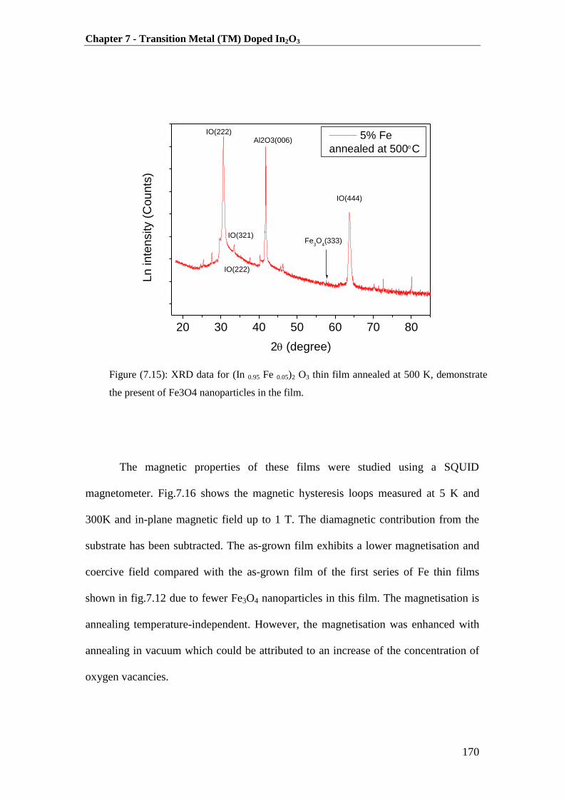
Chapter 7 - Transition Metal (TM) Doped In2O3
170
The magnetic properties of these films were studied using a SQUID
magnetometer. Fig.7.16 shows the magnetic hysteresis loops measured at 5 K and
300K and in-plane magnetic field up to 1 T. The diamagnetic contribution from the
substrate has been subtracted. The as-grown film exhibits a lower magnetisation and
coercive field compared with the as-grown film of the first series of Fe thin films
shown in fig.7.12 due to fewer Fe3O4 nanoparticles in this film. The magnetisation is
annealing temperature-independent. However, the magnetisation was enhanced with
annealing in vacuum which could be attributed to an increase of the concentration of
oxygen vacancies.
Figure (7.15): XRD data for (In 0.95 Fe 0.05)2 O3 thin film annealed at 500 K, demonstrate
the present of Fe3O4 nanoparticles in the film.
20 30 40 50 60 70 80
IO(444)
Fe3O
4(333)
Al2O3(006)
IO(222)
IO(321)
IO(222)
Ln
in
ten
sity (
Co
un
ts)
2 (degree)
5% Fe
annealed at 500C

Chapter 7 - Transition Metal (TM) Doped In2O3
171
The influence of Sn doping on Fe-doped In2O3 films was investigated, where
three films of (In0.95-y Fe0.05 Sny)2 O3 were grown with y = 0, 0.05 and 0.1. The films
were grown in KACST under the same growth conditions. Fig.7.17 shows the
magnetic hysteresis loop at 5 K and 300 K measured by the SQUID under a magnetic
field of 1 T. The magnetic moment decreases with increases of n concentration which
could be due to prevent the formation of the nanoparticles in the films.
The MCD spectra of these films were measured at room temperature in
applied magnetic field up to 1.8 T as shown in fig.7.18. The spectra show a peak at
about 2.2 eV for the pure Fe-doped In2O3 films whereas the peak has totally
disappeared for the films with 5% and 10% tin (Sn). As found previously that the Fe-
doped In2O3 film contains Fe3O4 nanoparticles this means that the peak shown in the
Fe-doped In2O3 films is due to the Fe3O4 nanoparticles. Adding tin leads to the
disappearance of the peaks at 2.2 eV which is in agreement with the magnetic data
shown in fig.7.17.
-10000 -5000 0 5000 10000-20
-15
-10
-5
0
5
10
15
20
0
-9
0
9
em
u/c
m3
Oe
300K
No Annealing
annealing at 500K
annealing at 400K
annealing at 300K
Ma
gn
etisa
tio
n(e
mu
/cm
3)
Magnetic field (Oe)
-10000 -5000 0 5000 10000-20
-15
-10
-5
0
5
10
15
20
0
-10
0
10
em
u/c
m3
Oe
No Annealing
annealing at 500K
annealing at 400K
annealing at 300K
5K
Mag
ne
tisatio
n (
em
u/c
m3)
Magnetic field (Oe)
Figure (7.16): The hysteresis loops measured at 5 K and 300 K of the as-grown and
annealed (In0.95 Fe0.05)2O3 thin films (the diamagnetic contribution from the substrate has
been subtracted). The Insets show the blow-up of the region around the origin.

Chapter 7 - Transition Metal (TM) Doped In2O3
172
-10000 -5000 0 5000 10000-15
-10
-5
0
5
10
15
-700 0 700
-5
0
Magnetis
atio
n (
em
u/c
m3)
Magneic field (Oe)
5K
Ma
gn
etisa
tion
(em
u/c
m3)
Magneic field (Oe)
5% Fe
5% Fe+5% Sn
5% Fe+10% Sn
-10000 -5000 0 5000 10000-15
-10
-5
0
5
10
15 5% Fe
5% Fe+5% Sn
5% Fe+10% Sn
-600 0 600
0
Magnetis
atio
n(e
mu/c
m3)
Magnetic field (Oe)
300K
Ma
gn
etisa
tio
n(e
mu
/cm
3)
Magnetic field (Oe)
Figure 7.17: The hysteresis loops measured at 5 K and 300 K of pure (In0.95 Fe0.05)2O3 thin films
and films doped with 5% and 10% Sn (the diamagnetic contribution from the substrate has been
subtracted). The Insets show the blow-up of the region around the origin.
Figure 7.18: Room temperature MCD spectra taken at 1.8 T of pure (In0.95 Fe0.05)2O3 thin
films and films doped with 5% and 10% Sn (the substrate contribution from has been
subtracted).

Chapter 7 - Transition Metal (TM) Doped In2O3
173
The MCD spectra also show a feature at 3.4 eV which increased with tin
doping due to the increase of the carrier concentration in the films. Both magnetic and
MCD data give good evidence that adding Sn to the Fe-doped In2O3 films leads to the
prevention of the formation of the nanoparticles where adding Sn may help the Fe
atom to substitute the In2O3 lattice rather than forming cluster or nanoparticles.
The second group of Fe-doped In2O3 thin films was grown to optimize the
growth processes and to study the magnetic and magneto-optic properties. Two thin
films of (In0.95 Fe0.05)2 O3 were grown at mTorr and 100 mTorr by PLD
technique in Xiao-Hong Xu’s group, China. The target was prepared for the PLD
from high-purity In2O3 (99.995%) and Fe2O3 (99.998%) powders. The stoichiometric
mixture was annealed in air at 500, 650 and 800 for 12 hours. The calcined powder
was then pressed and sintered in air at 1100 for 12 hours and the resultant pellet
was used as a target in the PLD. The films were deposited on a sapphire substrate at
600 by PLD with energy of 300 mJ/pulse. The data presented in this section of
these films have been published in [4].
The XRD patterns of (In0.95 Fe0.05)2 O3 film grown at mTorr can be
shown in fig.7.19, measured by Xu in in Shanxi Normal University Linfen, China.
The XRD pattern shows high crystalline with single phase cubic structure and well-
orinted (222) as the un-doped In2O3 structure. No secondary phases relating to
metallic Fe clusters or Fe oxide are observed which indicates that Fe ions are
substituted in to the In3+
sites of the In2O3 lattice without changing the cubic bixbyite
structure. This result is totally different to that found for the film grown in KACST
shown in fig.7.9.

Chapter 7 - Transition Metal (TM) Doped In2O3
174
Removed by the
author for copyright reasons
Measurements of the magnetic properties of these films were made with a
SQUID magnetometer. Fig.7.20 shows the magnetic hysteresis loops measured at 5 K
and 300K for (In 0.95 Fe0.05)2 O3 films grown at mTorr and 100 mTorr. The
diamagnetic contribution from the substrate has been subtracted as shown in the
insets. The samples illustrate a clear room temperature (RT) ferromagnetic behaviour.
The magnetisation of the film deposited at mTorr is independent of
temperature, which strongly indicates that the Tc of the film is above room
temperature. This is therefore essential for developing practical spintronic devices. In
contrast, the magnetisation of the film deposited at 100 mTorr displays temperature
dependent behaviour and the magnetisation is relatively small which suggests the
presence of a paramagnetic contribution in the film besides the ferromagnetic
moment.
Figure (7.19): XRD data of (In 1-x Fe x) 2O3, shows the patterns of (In0.95 Fe0.05)2O3
grown at mTorr [4].

Chapter 7 - Transition Metal (TM) Doped In2O3
175
Removed by the
author for copyright reasons
The expected paramagnetic susceptibility per volume ( ) from the Fe2+
ions
at 5 K was calculated using
where is the effective number
of Bohr magnetons ( ), N is the number of host ions per cm3 and is the Fe
2+
concentration. The peff of Fe2+
is taken only for the spin value of p= 4.90 which is for
the low symmetry that is give fully quench of the orbital contribution. The measured
values of Curie constant Cmeas and the calculated values C of the Fe2+
of these films
are given in the Table (7.2). The Curie constant values measured for both films were
close to the expected values for Fe2+
. This result indicates that the Fe ions in the film
are Fe2+
and all the Fe2+
ions in the films are paramagnetic. This result is similar to
what have been found for Co2+
ions shown in fig.7.6.
Figure (7.20): The hysteresis loops measured at 5K and 300K of (In0.95 Fe0.05)2O3 thin films
deposited under various oxygen pressure of a) mTorr and b) 100 mTorr (the
diamagnetic contribution from the substrate has been subtracted). The Insets show the blow-
up of the region around the origin [4].

Chapter 7 - Transition Metal (TM) Doped In2O3
176
Film
thickness
(nm)
Oxygen
Pressure
(mTorr)
( /V)meas
×10-3
Cmeas
×10-3
( /V)
×10-3
Ccalc
×10-3
319 5 10-5
1.28 6.40 1.46 7.31
224 100 1.43 7.14 1.46 7.31
Table (7.2): Summary of the paramagnetic susceptibility ( ) and Curie constant measured
values of (In0.95 Fe0.05)2O3 thin films and the expected values of Fe2+
ions respectively.
The transport properties of these films were measured by Xu using four-pont
configuration. Fig.7.21 shows the temperature dependence of resistance (R) of
(In0.95 Fe0.05)2 O3 films grown at mTorr and 100 mTorr. This plot indicates
metallic behaviour of the film grown at mTorr whereas the film grown at
100 mTorr shows classic semiconductor behaviour. This illustrates that the oxygen
partial pressure effects on the resistivity and then on carrier density due to the
variation in the number of Fe2+
ions or the density of the Oxygen vacancies.
Therefore, the difference in the ferromagnetic behaviour between the film grown at
mTorr and the one grown at 100 mTorr exists because that the former film
lies in the metallic regime and the later one lies in the insulating regime.

Chapter 7 - Transition Metal (TM) Doped In2O3
177
Removed by the
author for copyright reasons
Figure (7.21): Resistance temperature dependence for the two (In0.95 Fe0.05)2O3 thin films
grown at mTorr and 100mTorr. The inset is Log RVs T1/4
for the film grown at
100mTorr [4].
In order to verify the origin of the magnetism the MCD spectroscopy were
measured for these films. Fig.7.22 shows the MCD spectra of (In0.95 Fe0.05)2 O3 films
measured at room temperature in applied magnetic field up to 1.8 Tesla perpendicular
to surface of the films. The contribution from the substrate has been subtracted from
the MCD spectra.
Fig.7.22 shows a positive signal for the film grown at mTorr around
the band edge whereas the film grown at 100 mTorr exhibits no MCD signal.
Moreover, the film grown at mTorr shows a contribution from the
forbidden transitions on the energy ranges 2.75 E 3.70 which is absent in the film
grown at high oxygen atmosphere (100 mTorr). This is because the former film is
metallic and contains a fraction of Fe2+
ions and these ions act as acceptors which
generate a spin polarized conduction band. Hence any exchange splitting in the
Chapter 7 - Transition Metal (TM) Doped In2O3
178
conduction band state will leads to a large imbalance in the density of states at Fermi
level which causes the strong MCD signal in the film grown at mTorr. In
contrast the film grown at high oxygen atmosphere (100 mTorr) is semiconducting
and had few carriers or contained a very few Fe2+
. In this film the states near the
Fermi level are localized and the density of states is potential dependent and energy
independent. Therefore, any spin splitting of these localized states will not lead to
unequal densities at the Femi level and as a result the MCD signal is very low which
could be below the experimental limit.
Removed by the
author for copyright reasons
Figure (7.22): Room temperature MCD spectra taken at 1.8T of (In 0.95 Fe0.05)2O3 thin films
grown at grown at mTorr and 100 mTorr [4].
Chapter 7 - Transition Metal (TM) Doped In2O3
179
7.4 Summary and Conclusions
This chapter reported the investigation of the magnetic and magneto-optical
properties of Co and Fe-doped In2O3. Ferromagnetic beyond room temperature was
found in Co and Fe-doped In2O3 films grown in two different research group using
different techniques. The investigation of XRD and EXAFS indicated that TM ions in
the films are predominately TM2+
and substitute for In3+
rather than forming a defect
phase. In this work the major emphasis is focused on exploring the contribution of the
TM to the magnetisation in order to determine the origin of ferromagnetism in this
system. A new simple method was established and the use this method illustrated that
the TM2+
ions are paramagnetic and do not contribution to the ferromagnetic moment
of the films.
The magneto-optics measurement showed a positive contribution from the
forbidden transition in the energy range eV for (In1-xCox)2O3 and
(In1-x Fex)2O3 thin films grown at low oxygen pressure and this transition is absent for
the films grown at high oxygen pressure. This is good evidence for a donor state
formed in the band gap energy of In2O3 and located closed to conduction band.
Oxygen vacancies are found to be the origin of these donor states which were
calculated to lay at 0.9 eV below the conduction band.
The magnetic and magneto-optics measurement together gives convincing
evidence that the magnetism observed in these films is due to the polarised electrons
in localised donor state and to the oxygen vacancies. Oxygen partial pressure plays a
crucial role for the carrier concentration and the density of oxygen vacancies. Hence a
decrease of oxygen partial pressure leads to an increase of the density of oxygen
vacancies and vice versa.

Chapter 7 - Transition Metal (TM) Doped In2O3
180
The (In1-x Fex)2O3 films grown in KACST by PLD contain a fraction of Fe3O4
nanoparticles whereas Fe ions substitute for In3+
in Fe-doped In2O3 films grown by
PLD in Xu group. This indicates that the TM doped In2O3 is very sensitive to the
growth method. The formation of Fe3O4 nanoparticles could be attributed to either the
grinding of the powder used to make the target or to the temperatures that were
involved in annealing the powder. However, adding Sn to the Fe-doped In2O3 films
may help to reduce the formation of Fe3O4 nanoparticles.

Chapter 7 - Transition Metal (TM) Doped In2O3
181
7.5 References
1. A. M. H. R. Hakimi, M. G. Blamire, S. M. Heald, M. S. Alshammari, M. S.
Alqahtani, D. S. Score, H. J. Blythe, A. M. Fox and G. A. Gehring, Physical
Review B 84 (8), 085201 (2011).
2. M. Venkatesan, R. D. Gunning, P. Stamenov and J. M. D. Coey, Journal of
Applied Physics 103 (7), 07D135-133 (2008).
3. X.-H. Xu, F.-X. Jiang, J. Zhang, X.-C. Fan, H.-S. Wu and G. A. Gehring,
Applied Physics Letters 94 (21), 212510-212513 (2009).
4. F.-X. Jiang, X.-H. Xu, J. Zhang, X.-C. Fan, H.-S. Wu, M. Alshammari, Q.
Feng, H. J. Blythe, D. S. Score, K. Addison, M. Al-Qahtani and G. A.
Gehring, Journal of Applied Physics 109 (5), 053907-053907 (2011).
5. T. Fukumura, H. Toyosaki and Y. Yamada, Semiconductor Science and
Technology 20 (4), S103 (2005).
6. S. B. Ogale, R. J. Choudhary, J. P. Buban, S. E. Lofland, S. R. Shinde, S. N.
Kale, V. N. Kulkarni, J. Higgins, C. Lanci, J. R. Simpson, N. D. Browning, S.
Das Sarma, H. D. Drew, R. L. Greene and T. Venkatesan, Physical Review
Letters 91 (7), 077205 (2003).
7. T. Fukumura, Z. Jin, A. Ohtomo, H. Koinuma and M. Kawasaki, Applied
Physics Letters 75 (21), 3366-3368 (1999).
8. Y. Matsumoto, M. Murakami, T. Shono, T. Hasegawa, T. Fukumura, M.
Kawasaki, P. Ahmet, T. Chikyow, S.-y. Koshihara and H. Koinuma, Science
291 (5505), 854-856 (2001).
9. C. B. Fitzgerald, M. Venkatesan, A. P. Douvalis, S. Huber, J. M. D. Coey and
T. Bakas, Journal of Applied Physics 95 (11), 7390-7392 (2004).

Chapter 7 - Transition Metal (TM) Doped In2O3
182
10. J. Philip, N. Theodoropoulou, G. Berera, J. S. Moodera and B. Satpati,
Applied Physics Letters 85 (5), 777-779 (2004).
11. H. Kim, M. Osofsky, M. M. Miller, S. B. Qadri, R. C. Y. Auyeung and A.
Pique, Applied Physics Letters 100 (3), 032404-032403 (2012).
12. D. Bérardan, E. Guilmeau and D. Pelloquin, Journal of Magnetism and
Magnetic Materials 320 (6), 983-989 (2008).
13. L. M. Huang, C. M. Araujo and R. Ahuja, Epl 87 (2) (2009).
14. H. W. Ho, B. C. Zhao, B. Xia, S. L. Huang, J. G. Tao, A. C. H. Huan and L.
Wang, Journal of Physics-Condensed Matter 20 (47) (2008).
15. Sub, iacute, G. as, J. Stankiewicz, F. Villuendas, M. Lozano, P. a, Garc and J.
a, Physical Review B 79 (9), 094118 (2009).
16. J. Philip, A. Punnoose, B. I. Kim, K. M. Reddy, S. Layne, J. O. Holmes, B.
Satpati, P. R. LeClair, T. S. Santos and J. S. Moodera, Nat Mater 5 (4), 298-
304 (2006).
17. G. Z. Xing, J. B. Yi, D. D. Wang, L. Liao, T. Yu, Z. X. Shen, C. H. A. Huan,
T. C. Sum, J. Ding and T. Wu, Physical Review B 79 (17), 174406 (2009).
18. R. P. Panguluri, P. Kharel, C. Sudakar, R. Naik, R. Suryanarayanan, V. M.
Naik, A. G. Petukhov, B. Nadgorny and G. Lawes, Physical Review B 79
(16), 165208 (2009).
19. G. Subías, J. Stankiewicz, F. Villuendas, M. P. Lozano and J. García, Physical
Review B 79 (9), 094118 (2009).
20. Y. K. Yoo, Q. Xue, H.-C. Lee, S. Cheng, X. D. Xiang, G. F. Dionne, S. Xu, J.
He, Y. S. Chu, S. D. Preite, S. E. Lofland and I. Takeuchi, Applied Physics
Letters 86 (4), 042506-042503 (2005).

Chapter 7 - Transition Metal (TM) Doped In2O3
183
21. O. D. Jayakumar, I. K. Gopalakrishnan, S. K. Kulshreshtha, A. Gupta, K. V.
Rao, D. V. Louzguine-Luzgin, A. Inoue, P. A. Glans, J. H. Guo, K. Samanta,
M. K. Singh and R. S. Katiyar, Applied Physics Letters 91 (5), 052504-
052503 (2007).
22. D. Chu, Y.-P. Zeng, D. Jiang and Z. Ren, Applied Physics Letters 91 (26),
262503-262503 (2007).
23. P. F. Xing, Y. X. Chen, S.-S. Yan, G. L. Liu, L. M. Mei, K. Wang, X. D. Han
and Z. Zhang, Applied Physics Letters 92 (2), 022513-022513 (2008).
24. F.-X. Jiang, X.-H. Xu, J. Zhang, H.-S. Wu and G. A. Gehring, Applied
Surface Science 255 (6), 3655-3658 (2009).
25. H. W. Ho, B. C. Zhao, B. Xia, S. L. Huang, Y. Wu, J. G. Tao, A. C. H. Huan
and L. Wang, Journal of Physics: Condensed Matter 20 (47), 475204 (2008).
26. N. H. Hong, J. Sakai, N. T. Huong, A. Ruyter and V. Brize, Journal of
Physics-Condensed Matter 18 (29), 6897-6905 (2006).
27. I. Hamberg, C. G. Granqvist, K. F. Berggren, B. E. Sernelius and L. Engström,
Physical Review B 30 (6), 3240-3249 (1984).
28. C. Nunes de Carvalho, G. Lavareda, A. Amaral, O. Conde and A. R. Ramos,
Journal of Non-Crystalline Solids 352 (23–25), 2315-2318 (2006).
29. J.-H. Lee, S.-Y. Lee and B.-O. Park, Materials Science and Engineering: B
127 (2–3), 267-271 (2006).
30. J. Stankiewicz, F. Villuendas, J. Bartolomé and J. Sesé, Journal of Magnetism
and Magnetic Materials 310 (2, Part 3), 2084-2086 (2007).
31. J. Stankiewicz, F. Villuendas, Bartolom, eacute and Juan, Physical Review B
75 (23), 235308 (2007).
Chapter 7 - Transition Metal (TM) Doped In2O3
184
32. A. M. H. R. Hakimi, F. Schoofs, R. Bali, N. A. Stelmashenko, M. G. Blamire,
S. Langridge, S. A. Cavill, G. van der Laan and S. S. Dhesi, Physical Review
B 82 (14), 144429 (2010).
33. T. Thomas, G. Milan, S. Gisela, J. Gerhard, B. Sebastian and G. Eberhard,
New Journal of Physics 10 (5), 055009 (2008).
34. A. Ney, K. Ollefs, S. Ye, T. Kammermeier, V. Ney, T. C. Kaspar, S. A.
Chambers, F. Wilhelm and A. Rogalev, Physical Review Letters 100 (15),
157201 (2008).
35. A. Barla, G. Schmerber, E. Beaurepaire, A. Dinia, H. Bieber, S. Colis, F.
Scheurer, J. P. Kappler, P. Imperia, F. Nolting, F. Wilhelm, A. Rogalev, D.
Müller and J. J. Grob, Physical Review B 76 (12), 125201 (2007).
36. Z. G. Yu, J. He, S. Xu, Q. Xue, O. M. J. van’t Erve, B. T. Jonker, M. A.
Marcus, Y. K. Yoo, S. Cheng and X.-d. Xiang, Physical Review B 74 (16),
165321 (2006).
37. L. X. Guan, J. G. Tao, Z. R. Xiao, B. C. Zhao, X. F. Fan, C. H. A. Huan, J. L.
Kuo and L. Wang, Physical Review B 79 (18), 184412 (2009).
38. J. He, S. Xu, Y. K. Yoo, Q. Xue, H.-C. Lee, S. Cheng, X. D. Xiang, G. F.
Dionne and I. Takeuchi, Applied Physics Letters 86 (5), 052503-052503
(2005).
39. J. Stankiewicz, F. Villuendas and J. Bartolomé, Physical Review B 75 (23),
235308 (2007).
40. J. R. Neal, A. J. Behan, R. M. Ibrahim, H. J. Blythe, M. Ziese, A. M. Fox and
G. A. Gehring, Physical Review Letters 96 (19), 197208 (2006).
41. K. Ando, H. Saito, Z. Jin, T. Fukumura, M. Kawasaki, Y. Matsumoto and H.
Koinuma, Applied Physics Letters 78 (18), 2700-2702 (2001).
Chapter 7 - Transition Metal (TM) Doped In2O3
185
42. A. J. Behan, J. R. Neal, R. M. Ibrahim, A. Mokhtari, M. Ziese, H. J. Blythe, A.
M. Fox and G. A. Gehring, Journal of Magnetism and Magnetic Materials 310
(2, Part 3), 2158-2160 (2007).
43. F.-X. Jiang, X.-H. Xu, J. Zhang, X.-C. Fan, H.-S. Wu and G. A. Gehring,
Applied Physics Letters 96 (5), 052503-052503 (2010).
44. S. M. Heald, T. Kaspar, T. Droubay, V. Shutthanandan, S. Chambers, A.
Mokhtari, A. J. Behan, H. J. Blythe, J. R. Neal, A. M. Fox and G. A. Gehring,
Physical Review B 79 (7), 075202 (2009).
45. D. A. Schwartz, N. S. Norberg, Q. P. Nguyen, J. M. Parker and D. R.
Gamelin, Journal of the American Chemical Society 125 (43), 13205-13218
(2003).
46. A. Walsh, J. L. F. Da Silva, S.-H. Wei, C. Körber, A. Klein, L. F. J. Piper, A.
DeMasi, K. E. Smith, G. Panaccione, P. Torelli, D. J. Payne, A. Bourlange and
R. G. Egdell, Physical Review Letters 100 (16), 167402 (2008).
47. L.-M. Tang, L.-L. Wang, D. Wang, J.-Z. Liu and K.-Q. Chen, Journal of
Applied Physics 107 (8), 083704-083705 (2010).
48. F. C. Fonseca, G. F. Goya, R. F. Jardim, R. Muccillo, N. L. V. Carreño, E.
Longo and E. R. Leite, Physical Review B 66 (10), 104406 (2002).

Chapter 8 - Conclusions and Future Work
186
Chapter 8
Conclusions and Future Work
8.1 Conclusions
This study has investigated the magnetic and magneto-optical properties of
LSMO, multiferroic GdMnO3 and TM-doped In2O3 thin films grown under different
conditions. Moreover, optical and magneto-optical measurements were made on a
STO substrate because it had been used to grow high quality thin films of LSMO and
GdMnO3 but it was found to have some disadvantages for an optical study. The
magnetic properties of each sample were measured in a SQUID and the magneto-
optical properties were performed in Faraday geometry.
8.1.1 LSMO Thin Films
The magnetic and magneto-optical properties of LSMO thin films grown on
both STO and sapphire substrate were studied. Increasing both the concentration of Sr
content and oxygen growth pressure shows an improvement of magnetic behaviour
for LSMO films grown on both STO and sapphire substrate. The ratio of Mn4+
/Mn3+
can be controlled by controlling the oxygen growth pressure. Therefore, increase of
oxygen pressure means increasing the number of holes in the films and thus
increasing the Mn4+
/Mn3+
ratio, and subsequently enhancing the magnetic properties
of LSMO films. In this study, It was found that the LSMO film of about 80nm
exhibits one of the highest values of TC=340 K compared to the previous studies [1-
2]. However, the reduction in the magnetisation in this film is attributed to the strain
Chapter 8 - Conclusions and Future Work
187
and interface between the film and the substrate [1].The value of so-called dead layer
is about 23 nm which is about 20 times higher than the previously reported dead layer
of 1.2 nm for LSMO on SrTiO3 (001) [3].
The strong MCD peak at the band gap at about 3.3 eV of the film grown on
sapphire was found to be shifted to lower energy with decreasing oxygen pressure
which could be attributed to the decrease of Mn4+
fraction and band width with
reduction in oxygen. The magnitude of the signal in the temperature dependence of
MCD measurement is found to be proportional to the polarisation of band electrons
which is needed in spintroncs. This result shows that a sapphire substrate is a
promising substrate for LSMO films for magneto-optical study. On the other hand, the
MCD spectrum of LSMO films on STO substrate are dominated by the magneto
optical properties and birefringence behaviour arising from the STO substrate. Hence,
the absorption of STO above its band gap at about 3.3 eV, its magneto-optical
properties and the birefringence are a limitation of the optical study of LSMO films.
The influence of birefringence on the magneto-optics of STO was
investigated. This study is considered the first attempt that investigated the influence
of birefringence on the magneto-optical properties of STO using the Sato method. It
was found that a STO substrate has a strongly temperature dependence of the MCD
below the band gap which also varied linearly with applied magnetic field. This result
indicates that it is not easy to study samples that are both birefringent and magnetic
and also that STO substrates are not suitable for optical studies. However magneto-
optical studies are a very powerful technique to study LSMO films.

Chapter 8 - Conclusions and Future Work
188
8.1.2 GdMnO3 Thin Films
The magnetic, optical and magneto-optical properties of epitaxial films of
GdMnO3 grown on SrTiO3 and LaAlO3 substrate were studied. This study is
considered the first attempt that investigated the magnetic and magneto-optical
properties of epitaxial GdMnO3 thin films. Considerable differences have been found
between the magnetic behaviour of bulk GdMnO3 and that grown on the two
substrates, STO and the twinned substrate of LAO. These apply different strains to the
manganite film. The Néel temperature is reduced and there is some evidence that a
canted phase appears with the onset of anti-ferromagnetism for both films.
The optical absorption data on these films was dominated by the strong
absorption that starts around 3 eV, but the 2 eV peak was not sufficiently strong to be
detected. However, both peaks featured strongly in the MCD data measured with thin
films of GdMnO3 grown on STO. The optical absorption at 3 eV is much stronger
than at 2 eV, but the MCD is considerably stronger at 2 eV. A dramatic result was the
stark difference between the shapes of the spectra taken in a field of 5kOe and at
remanence, as well as in the hysteresis loops. The 2 eV peak is attributed to the charge
transfer transition between Mn ions occurring near 2 eV, whereas the 3 eV peak is due
to the contribution from the STO substrate. Hence, the STO substrate exhibited a
MCD temperature dependenent signal at about 3 eV and this signal dominates the
MCD spectra, so that the MCD peak at 3 eV is due to the STO substrate. The
transition near 2 eV was more strongly dependent on temperature, but much less
sensitive to the external field, and was observed in the remnant spectrum. It was a
clear feature in the MCD, whereas it is strongly suppressed in the optical absorption.
This is because it depends so strongly on the spin dependence of the occupation of the
Mn d orbitals. It also depends on the relative orientation of the spins of the

Chapter 8 - Conclusions and Future Work
189
neighbouring Mn ions and on the Mn-O-Mn bond angle. It is clear that study of the
MCD spectrum of this material is a rich source of information that is not available
from a study of the magnetisation and the absorption alone.
8.1.3 Co and Fe- Doped In2O3 Thin Films
The magnetic and magneto-optical properties of Co and Fe-doped In2O3 thin
films were studied. The study showed that the RT ferromagnetic of (In1-x Cox)2O3 and
(In1-x Fex)2O3 thin films is ascribed to the substitution of Co and Fe ions for In ions
and not due to either the presence of metallic clusters or oxides secondary phases in
the films.
A new method was established to explore the contribution of the transition
metal ions (TM) to the magnetisation in order to determine the origin of
ferromagnetism in this system. This method was used to estimate the paramagnetic
contribution of the films at 5K and compare it with the expected paramagnetic
susceptibility from the TM ions which was calculated at the fully quenching of the
orbital angular momentum. This method revealed that the Co and Fe ions in (In1-
xCox)2O3 and (In1-xFex)2O3 thin films are paramagnetic and do not contribute to the
magnetisation. This result is in agreement with a X-ray magnetic circular dichroism
(XMCD) study reported previously for Zn1-xCoxO films [4-5] Co-doped indium tin
oxide (ITO) [6] and Mn doped ITO [7].
The study of magneto-optical properties of Co and Fe-doped In2O3 is
considered to be the first attempt on these materials. This study revealed that there are
donor states formed in the band gap energy of In2O3 and located closed to the
conduction band. The origin of these donor states is oxygen vacancies which were
calculated to lie at 0.9 eV below the conduction band [8-9]. The density of oxygen
Chapter 8 - Conclusions and Future Work
190
vacancies depends on the oxygen partial pressure and a decrease of oxygen partial
pressure leads to an increase in the number of the oxygen vacancies and vice versa.
The magnetic and magneto-optical properties together indicate that the observed
ferromagnetism in TM-doped In2O3 is due to the polarised electrons in localized
donor state associated with oxygen vacancies.
EXAFS measurement showed the existence of Fe3O4 nanoparticles in some of
Fe-doped In2O3 thin films. In this study, the calculation of the expected magnetisation
from Fe3O4 nanoparticles in the thin films supports the EXAFS result of existence the
Fe3O4 nanoparticles in these films. The existence of Fe3O4 nanoparticles in these films
are very probably due to the processing conditions of fabrication. This indicates that
the TM-doped In2O3 thin films are extremely sensitive to the fabrication method and
to the processing conditions. However, adding Sn to the Fe-doped In2O3 films could
lead to a reduction of the formation of Fe3O4 nanoparticles and may help the Fe atoms
to substitute the In2O3 lattice rather than forming cluster or nanoparticles.
8.2 Future Work
There are a number of unresolved issues that it would be interesting to pursue
in further work for LSMO and TM-doped In2O3 films.
The quality of LSMO thin-film is crucial for device performance. A high
quality LSMO thin film should exhibit a large magnetization, small residual resistivity
and smooth surface morphology and avoid surface segregation. The high quality
LSMO film can illustrate saturation magnetisation near to the expected
value where values of have observed previously in LSMO single crystals
[10] , polycrystals [11] and thin films [12]. It would be really interesting to grow
high-quality thin film of LSMO. This requires investigating the film with x-ray

Chapter 8 - Conclusions and Future Work
191
diffraction, atomic force microscopy, SQUID, van der Pauw configuration and
scanning transmission electron microscopy.
The TM-doped In2O3 thin films are very sensitive to the fabrication method
and processing conditions. The most important issue is to grow reproducible thin
films of TM-doped In2O3. This will need to investigate the growth conditions such as
the method of preparing and grinding the powder, effect of different precursor, and
plume quality. Further investigation is required on (V, Cr, Mn, Ni, Cu and Zn)-doped
In2O3 and tin-doped indium oxide (ITO). On the other hand, it would be very
interesting to grow high quality Fe-doped In2O3 for the application in devices. All
these together will provide for a deeper understanding of the origin of ferromagnetism
in DMS films.
Finally, since the discovery of graphene in 2004 [13], the electrical properties
of graphene have attracted much attention for voluminous fundamental studies. Most
of the recent research has focused on growth of large sheets of monolayer or bilayer
graphene [14]. Following interesting work on the magneto-optics studies of graphene
films in the infrared (IR) and noting that the Faraday rotation had been calculated for
graphite but never measured; we attempted to grow graphite on sapphire substrate
using PLD and spin coating but some difficulties were faced, which delayed the
project.

Chapter 8 - Conclusions and Future Work
192
8.3 Reference
1. A. K. Pradhan, D. Hunter, T. Williams, B. Lasley-Hunter, R. Bah, H. Mustafa,
R. Rakhimov, J. Zhang, D. J. Sellmyer, E. E. Carpenter, D. R. Sahu and J. L.
Huang, Journal of Applied Physics 103 (2), 023914-023918 (2008).
2. Y. P. Sukhorukov, A. P. Nosov, N. N. Loshkareva, E. V. Mostovshchikova, A.
V. Telegin, E. Favre-Nicolin and L. Ranno, Journal of Applied Physics 97
(10), 103710-103715 (2005).
3. M. Huijben, L. W. Martin, Y. H. Chu, M. B. Holcomb, P. Yu, G. Rijnders, D.
H. A. Blank and R. Ramesh, Physical Review B 78 (9) (2008).
4. A. Ney, K. Ollefs, S. Ye, T. Kammermeier, V. Ney, T. C. Kaspar, S. A.
Chambers, F. Wilhelm and A. Rogalev, Physical Review Letters 100 (15)
(2008).
5. A. Barla, G. Schmerber, E. Beaurepaire, A. Dinia, H. Bieber, S. Colis, F.
Scheurer, J. P. Kappler, P. Imperia, F. Nolting, F. Wilhelm, A. Rogalev, D.
Mueller and J. J. Grob, Physical Review B 76 (12) (2007).
6. A. M. H. R. Hakimi, F. Schoofs, R. Bali, N. A. Stelmashenko, M. G. Blamire,
S. Langridge, S. A. Cavill, G. van der Laan and S. S. Dhesi, Physical Review
B 82 (14), 144429 (2010).
7. M. Venkatesan, R. D. Gunning, P. Stamenov and J. M. D. Coey, Journal of
Applied Physics 103 (7) (2008).
8. L.-M. Tang, L.-L. Wang, D. Wang, J.-Z. Liu and K.-Q. Chen, Journal of
Applied Physics 107 (8), 083704-083705 (2010).
9. A. M. H. R. Hakimi, M. G. Blamire, S. M. Heald, M. S. Alshammari, M. S.
Alqahtani, D. S. Score, H. J. Blythe, A. M. Fox and G. A. Gehring, Physical
Review B 84 (8), 085201 (2011).

Chapter 8 - Conclusions and Future Work
193
10. A. Urushibara, Y. Moritomo, T. Arima, A. Asamitsu, G. Kido and Y. Tokura,
Physical Review B 51 (20), 14103-14109 (1995).
11. T. Koide, H. Miyauchi, J. Okamoto, T. Shidara, T. Sekine, T. Saitoh, A.
Fujimori, H. Fukutani, M. Takano and Y. Takeda, Physical Review Letters 87
(24), 246404 (2001).
12. H. Boschker, M. Huijben, A. Vailionis, J. Verbeeck, S. v. Aert, M. Luysberg,
S. Bals, G. v. Tendeloo, E. P. Houwman, G. Koster, D. H. A. Blank and G.
Rijnders, Journal of Physics D: Applied Physics 44 (20), 205001 (2011).
13. J. Hofrichter, B. N. Szafranek, M. Otto, T. J. Echtermeyer, M. Baus, A.
Majerus, V. Geringer, M. Ramsteiner and H. Kurz, Nano Letters 10 (1), 36-42
(2010).
14. Z. Sun, Z. Yan, J. Yao, E. Beitler, Y. Zhu and J. M. Tour, Nature 468 (7323),
549-552 (2010).

Appendix A
194
Appendix A
Chapter 6 – Appendix
The Sato method [1] was employed in order to discuss the magneto-optic
spectrum of the medium that exhibits magnetic and birefringent behaviour. At optical
frequencies, propagation of electromagnetic waves through a material can be
described in terms of the electric permeability tensors, [2]. For a crystal with cubic
symmetry magnetised perpendicularly to its surface, i.e., the z-direction, this dielectric
tensor tensors can be written in the form:
(
) A. 6.1
Where each element has real and imaginary part as:
A. 6.2
The diagonal elements are related to normal refractive index and
extinction coefficient. The off-diagonal element describes the magneto-optical effects
such as the Kerr effects and the Faraday effect. The dielectric tensor, , for an
isotropic magnetic medium with the magnetisation directed along the axis, can be
written as:
(
) A. 6.3
If the sample has a birefringence , the light transmitted through the sample can be
calculated by writing the dielectric tensor as following:

Appendix A
195
(
) A. 6.4
Here, is the birefringence, and the magnetism is included via the off-
diagonal term, . The eignestates of propagation are given in term of and :
(
) (
) A.6.5
A.6.6
√
A.6.7
√
A.6.8
√
A.6.9
The two values of the dielectric constant are given by:
√
) A.6.10
The refractive indices are given by:
√ √
√
)] A.6.11
The rotation () and ellipticity are evaluated respectively from:
√
√ A.6.12
Appendix A
196
√
√
√ √
A. 6.13
If the birefringence, Δ , is small. According to equation (6.11), we revert to the
standard result; otherwise the ellipticity is a maximum for a minimum value of Δ. The
aim, therefore, is to obtain the ellipticity from the birefringence (Δ) with as little
contamination as possible.
From the Sato method, and after detailed mathematics, the final intensity, after
passing through the Sato rig, is given by:
A. 6.14
A. 6.15
Where A=
, B= ,
and are Bessel functions. The coefficients and can be determined by the
calibration procedure.
The terms involving are odd under magnetic field reversal; and terms in are
even under magnetic field reversal and hence do not contribute in a magneto-optic
measurement. The measurements can be made both in a magnetic field and in zero
magnetic field. In the case of measurements made in a field (H), the difference
between the measurements for +H and –H is taken and only terms in remain:
[ (
)] A. 6.16
] ]] A. 6.17
Appendix A
197
If the measurement was taken in zero field then and should be zero.
Hence it is found that:
and
In this case, the
and
spectra are given by:
A.6.18
A.6.19
References
1. K. Sato, Japanese Journal of Applied Physics 20 (12), 2403-2409 (1981).
2. S. Wittekoek, T. J. A. Popma, J. M. Robertson and P. F. Bongers, Physical
Review B 12 (7), 2777-2788 (1975).