Imperial College LondonDepartment of Computing

Machine Learning with Chaotic RecurrentNeural Networks

Thomas Fonlladosa (tcf12)

September 2013

Supervised by Professor Murray Shanahan

Submitted in part fulfilment of the requirements for theMSc Degree in Advanced Computing of Imperial College London

Abstract

The aim of this project is to use some machine learning methods with continuous time recurrentneural networks that spontaneously exhibit chaotic behaviours and explore different applications.We first apply the training algorithms to learn the spontaneous or inputs-depending generation of

complex periodic patterns.Secondly, these results are applied to control a two joints robot arm. We also extend them to thepost-learning generation of new untaught patterns that matches new inputs by interpolation of

the trained behaviours.Thirdly a robust 2-bits working memory is implemented.

At last we train a network to generate complex aperiodic control signals that could be used tocontrol a drone trajectory on one dimension. In this part, a similar interpolation process leads to

the generation of new untaught signals.

1

Acknowledgements

I would like to thank Professor Murray Shanahan for the precious suggestions and guidelines hegave me during this project, as for the enthusiasm he showed about our results.

Thanks also to Thomas, Nicolas, Hugo, Diana, Nick, George, Marc-Antoine, Guillaume and theirflatmates for hosting me during the summer and thus making my work easier.Thanks to Julien-James my friend and proof-reader for his useful corrections.

Thanks to my friend Suzanne for her priceless moral support during the last weeks of this project.

2

Contents

Introduction 7

1 Background 81.1 Recurrent Neural Networks . . . . . . . . . . . . . . . . . . . . . . . . . . . . . . . . 81.2 Leaky integrator Model . . . . . . . . . . . . . . . . . . . . . . . . . . . . . . . . . . 81.3 Chaotic activity . . . . . . . . . . . . . . . . . . . . . . . . . . . . . . . . . . . . . . . 91.4 Reservoir Computing . . . . . . . . . . . . . . . . . . . . . . . . . . . . . . . . . . . . 91.5 Plasticity and learning in the biological brain . . . . . . . . . . . . . . . . . . . . . . 91.6 Learning in Recurrent Neural Networks . . . . . . . . . . . . . . . . . . . . . . . . . 10

1.6.1 FORCE learning . . . . . . . . . . . . . . . . . . . . . . . . . . . . . . . . . . 101.6.2 Reward modulated learning . . . . . . . . . . . . . . . . . . . . . . . . . . . . 101.6.3 Applications . . . . . . . . . . . . . . . . . . . . . . . . . . . . . . . . . . . . 10

2 Theory 122.1 Networks architectures . . . . . . . . . . . . . . . . . . . . . . . . . . . . . . . . . . . 12

2.1.1 Architecture A . . . . . . . . . . . . . . . . . . . . . . . . . . . . . . . . . . . 122.1.2 Architecture B . . . . . . . . . . . . . . . . . . . . . . . . . . . . . . . . . . . 132.1.3 Architecture C . . . . . . . . . . . . . . . . . . . . . . . . . . . . . . . . . . . 14

2.2 Learning Algorithms . . . . . . . . . . . . . . . . . . . . . . . . . . . . . . . . . . . . 142.2.1 FORCE learning . . . . . . . . . . . . . . . . . . . . . . . . . . . . . . . . . . 142.2.2 Reward Modulated Learning . . . . . . . . . . . . . . . . . . . . . . . . . . . 16

3 Implementation 183.1 Organisation . . . . . . . . . . . . . . . . . . . . . . . . . . . . . . . . . . . . . . . . 183.2 Create Network . . . . . . . . . . . . . . . . . . . . . . . . . . . . . . . . . . . . . . . 183.3 Train Network . . . . . . . . . . . . . . . . . . . . . . . . . . . . . . . . . . . . . . . 18

3.3.1 FORCE learning . . . . . . . . . . . . . . . . . . . . . . . . . . . . . . . . . . 183.3.2 Reward modulated learning . . . . . . . . . . . . . . . . . . . . . . . . . . . . 19

3.4 Run Network . . . . . . . . . . . . . . . . . . . . . . . . . . . . . . . . . . . . . . . . 193.4.1 Run network A-B-C . . . . . . . . . . . . . . . . . . . . . . . . . . . . . . . . 193.4.2 Drone simulation . . . . . . . . . . . . . . . . . . . . . . . . . . . . . . . . . . 19

3.5 Inputs/Outputs Definition . . . . . . . . . . . . . . . . . . . . . . . . . . . . . . . . . 193.5.1 Static inputs . . . . . . . . . . . . . . . . . . . . . . . . . . . . . . . . . . . . 193.5.2 Dynamic inputs . . . . . . . . . . . . . . . . . . . . . . . . . . . . . . . . . . . 203.5.3 Target functions . . . . . . . . . . . . . . . . . . . . . . . . . . . . . . . . . . 20

4 Generating periodic patterns 214.1 No input . . . . . . . . . . . . . . . . . . . . . . . . . . . . . . . . . . . . . . . . . . . 21

4.1.1 Single output . . . . . . . . . . . . . . . . . . . . . . . . . . . . . . . . . . . . 214.1.2 Multiple outputs . . . . . . . . . . . . . . . . . . . . . . . . . . . . . . . . . . 26

4.2 Input/output matching . . . . . . . . . . . . . . . . . . . . . . . . . . . . . . . . . . 274.3 Conclusion . . . . . . . . . . . . . . . . . . . . . . . . . . . . . . . . . . . . . . . . . 29

5 Application to a robot arm 315.1 Robot description . . . . . . . . . . . . . . . . . . . . . . . . . . . . . . . . . . . . . . 315.2 Matching inputs with different movements . . . . . . . . . . . . . . . . . . . . . . . . 325.3 Inputs interpolation to produce new movements . . . . . . . . . . . . . . . . . . . . . 36

3

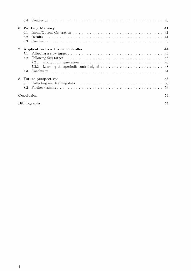
5.4 Conclusion . . . . . . . . . . . . . . . . . . . . . . . . . . . . . . . . . . . . . . . . . 40

6 Working Memory 416.1 Input/Output Generation . . . . . . . . . . . . . . . . . . . . . . . . . . . . . . . . . 416.2 Results . . . . . . . . . . . . . . . . . . . . . . . . . . . . . . . . . . . . . . . . . . . . 416.3 Conclusion . . . . . . . . . . . . . . . . . . . . . . . . . . . . . . . . . . . . . . . . . 43

7 Application to a Drone controller 447.1 Following a slow target . . . . . . . . . . . . . . . . . . . . . . . . . . . . . . . . . . . 447.2 Following fast target . . . . . . . . . . . . . . . . . . . . . . . . . . . . . . . . . . . . 46

7.2.1 input/ouput generation . . . . . . . . . . . . . . . . . . . . . . . . . . . . . . 467.2.2 Learning the aperiodic control signal . . . . . . . . . . . . . . . . . . . . . . . 48

7.3 Conclusion . . . . . . . . . . . . . . . . . . . . . . . . . . . . . . . . . . . . . . . . . 51

8 Future perspectives 538.1 Collecting real training data . . . . . . . . . . . . . . . . . . . . . . . . . . . . . . . . 538.2 Further training . . . . . . . . . . . . . . . . . . . . . . . . . . . . . . . . . . . . . . . 53

Conclusion 54

Bibliography 54

4

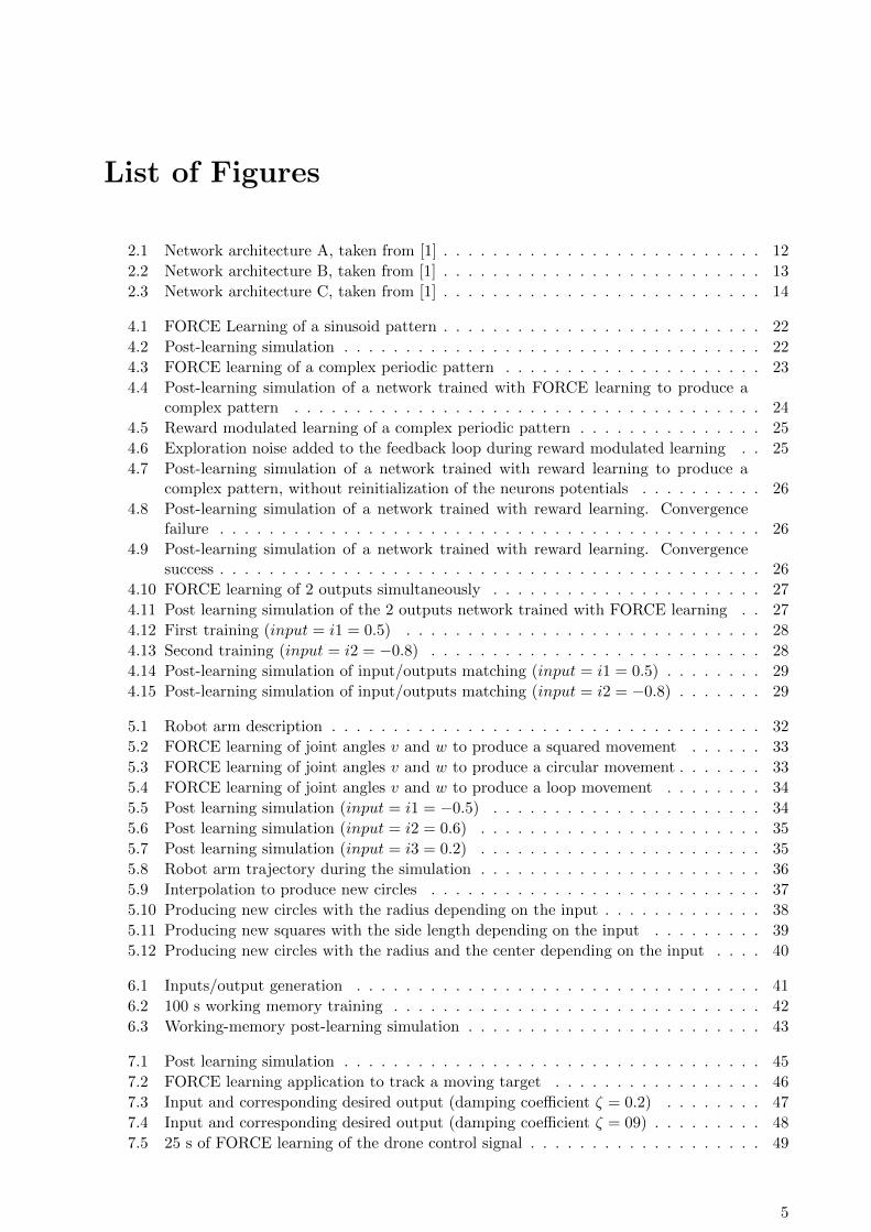
List of Figures

2.1 Network architecture A, taken from [1] . . . . . . . . . . . . . . . . . . . . . . . . . . 12

2.2 Network architecture B, taken from [1] . . . . . . . . . . . . . . . . . . . . . . . . . . 13

2.3 Network architecture C, taken from [1] . . . . . . . . . . . . . . . . . . . . . . . . . . 14

4.1 FORCE Learning of a sinusoid pattern . . . . . . . . . . . . . . . . . . . . . . . . . . 22

4.2 Post-learning simulation . . . . . . . . . . . . . . . . . . . . . . . . . . . . . . . . . . 22

4.3 FORCE learning of a complex periodic pattern . . . . . . . . . . . . . . . . . . . . . 23

4.4 Post-learning simulation of a network trained with FORCE learning to produce acomplex pattern . . . . . . . . . . . . . . . . . . . . . . . . . . . . . . . . . . . . . . 24

4.5 Reward modulated learning of a complex periodic pattern . . . . . . . . . . . . . . . 25

4.6 Exploration noise added to the feedback loop during reward modulated learning . . 25

4.7 Post-learning simulation of a network trained with reward learning to produce acomplex pattern, without reinitialization of the neurons potentials . . . . . . . . . . 26

4.8 Post-learning simulation of a network trained with reward learning. Convergencefailure . . . . . . . . . . . . . . . . . . . . . . . . . . . . . . . . . . . . . . . . . . . . 26

4.9 Post-learning simulation of a network trained with reward learning. Convergencesuccess . . . . . . . . . . . . . . . . . . . . . . . . . . . . . . . . . . . . . . . . . . . . 26

4.10 FORCE learning of 2 outputs simultaneously . . . . . . . . . . . . . . . . . . . . . . 27

4.11 Post learning simulation of the 2 outputs network trained with FORCE learning . . 27

4.12 First training (input = i1 = 0.5) . . . . . . . . . . . . . . . . . . . . . . . . . . . . . 28

4.13 Second training (input = i2 = −0.8) . . . . . . . . . . . . . . . . . . . . . . . . . . . 28

4.14 Post-learning simulation of input/outputs matching (input = i1 = 0.5) . . . . . . . . 29

4.15 Post-learning simulation of input/outputs matching (input = i2 = −0.8) . . . . . . . 29

5.1 Robot arm description . . . . . . . . . . . . . . . . . . . . . . . . . . . . . . . . . . . 32

5.2 FORCE learning of joint angles v and w to produce a squared movement . . . . . . 33

5.3 FORCE learning of joint angles v and w to produce a circular movement . . . . . . . 33

5.4 FORCE learning of joint angles v and w to produce a loop movement . . . . . . . . 34

5.5 Post learning simulation (input = i1 = −0.5) . . . . . . . . . . . . . . . . . . . . . . 34

5.6 Post learning simulation (input = i2 = 0.6) . . . . . . . . . . . . . . . . . . . . . . . 35

5.7 Post learning simulation (input = i3 = 0.2) . . . . . . . . . . . . . . . . . . . . . . . 35

5.8 Robot arm trajectory during the simulation . . . . . . . . . . . . . . . . . . . . . . . 36

5.9 Interpolation to produce new circles . . . . . . . . . . . . . . . . . . . . . . . . . . . 37

5.10 Producing new circles with the radius depending on the input . . . . . . . . . . . . . 38

5.11 Producing new squares with the side length depending on the input . . . . . . . . . 39

5.12 Producing new circles with the radius and the center depending on the input . . . . 40

6.1 Inputs/output generation . . . . . . . . . . . . . . . . . . . . . . . . . . . . . . . . . 41

6.2 100 s working memory training . . . . . . . . . . . . . . . . . . . . . . . . . . . . . . 42

6.3 Working-memory post-learning simulation . . . . . . . . . . . . . . . . . . . . . . . . 43

7.1 Post learning simulation . . . . . . . . . . . . . . . . . . . . . . . . . . . . . . . . . . 45

7.2 FORCE learning application to track a moving target . . . . . . . . . . . . . . . . . 46

7.3 Input and corresponding desired output (damping coefficient ζ = 0.2) . . . . . . . . 47

7.4 Input and corresponding desired output (damping coefficient ζ = 09) . . . . . . . . . 48

7.5 25 s of FORCE learning of the drone control signal . . . . . . . . . . . . . . . . . . . 49

5

7.6 Network simulation on unseen input values (the desired trajectory and the associatedcontrol signal are produced with a damping coefficient ζ = 0.5) . . . . . . . . . . . . 50

7.7 Network simulation on unseen input values (the desired trajectory and the associatedcontrol signal are produced with a damping coefficient ζ = 0.9) . . . . . . . . . . . . 51

6

Introduction

Recurrent neural networks are different from feed-forward networks because their recurrent con-nectivity give them internal states allowing to exhibit dynamical behaviours. The dynamic of suchnetworks depends on the inputs they receive as well as on their previous state. This particularityof recurrent networks to be able to produce a wide range of dynamical behaviours has a lot ofapplications. They are also a source of interest because some models of recurrent neural networkscan be a good representation of biological brains.Two recent publications ([1] and [2]) describe how recurrent neural networks that spontaneouslyexhibit chaotic behaviour can be trained with different learning algorithms to produce some com-putational structures such as a working memory or to generate some complex periodic patterns.Those two papers are our main source of inspiration for this project: in this thesis, after havingreplicated some of their results, we tried to go further and explore new areas of application of suchnetworks.

The first chapter of this report presents the background of the thesis.The second chapter presents formally the network architectures and the learning algorithms thatare applied to them in this project.The third chapter gives some details of the matlab implementation.The fourth chapter describes the first results, ie the generation of periodic patterns.The fifth chapter explains the application of the first results to a two-joints robot arm, and theinterpolation process which is introduced to learn new patterns.The sixth chapter is about the implementation of a robust 2-bits memory.The seventh chapter deals with the learning of complex aperiodic control-signals within the frame-work of an application to a drone controller.The eighth chapter finally describes the future perspectives that could follow this project regardingthe previous chapter in particular.

7

1 Background

Labyrinthe sans clef ! ...

1.1 Recurrent Neural Networks

In this project, we are using a generic network of N neurons who are sparsely randomly recur-rently connected by excitatory and inhibitory synapses. This general architecture with sparse andasymmetric connections has often been used to model the dynamic activity of recurrent biologicalneural networks ([1], [3]). The neurons can also receive external inputs. Some read-out units per-form a linear combination of the neurons activity to generate an output. The network output(s) issometime fed back to the network, directly or via a second feedback network.

1.2 Leaky integrator Model

Each network unit i is a leaky integrator. In this model, the membrane potential xi of each neuroni follows a variant of this first order differential equations, which depends on the particular networkarchitecture that is used (cf 2.1 for the details of the different network architectures):

τ xi(t) = −xi(t) + λN∑i=1

W recij rj(t) +

M∑i=1

W inij Ij(t) +

L∑i=1

W zijzj(t)

where

• τ is the time constant (we can assume it is the same for all units)

• xi is the neuron’s membrane potential

• λ is a scaling factor on the recurrent connection whose value can introduce chaotic dynamicin the network.

• W recij is the synaptic weight from neuron j to i for the recurrent network

• rj = tanh(xj(t)) is the firing rate of the jth neuron.

• W inij is the weight of the incoming current Ij(t) in i.

• W zij is the weight applied to the read-out unit j when fed back to neuron i.

• zj is the output of the readout unit j.

In fact, each neuron can been seen as a RC circuit, and the differential equations are derived fromKirchoff’s current law that says that the total current flowing toward any node of an electricalcircuit is zero [4]. This model of integrate and fire neurons ignores inter-neuron propagation times.There exists some more biologically plausible neuron models like Izhikevich or Hodgkins-Huxleymodels that have a larger repertoire of behaviours but are also more computationally expensive.

8

1.3 Chaotic activity

The dynamic of such neural networks, also called continuous-time recurrent neural networks hasbeen studied in details, and they have a lot of applications [5]. Because of delayed effects impliedby the use of recurrent connections and feedback loops, such networks can spontaneously exhibitchaotic activity.The transition from a stationary to a chaotic state occur at a critical value of the gain parameterλ [6]. At the transition between chaos and stability, neural networks can produce complex compu-tational tasks. [7].Experimental results showed that spontaneously chaotic networks are easier to train and producemore accurate and robust outputs than non chaotic networks. The more a network is chaotic thebetter is the training, however with an upper bound ([1]).

1.4 Reservoir Computing

Reservoir computing is a framework that gives a way of designing and training recurrent neuralnetworks. It is a good model for biological networks. The main characteristic of reservoir comput-ing as describe in [8] are mainly:

• the use of a reservoir which is a large randomly connected recurrent neural network thatcan be excited by input signals. The reservoir maps the input to a higher dimensional spacebecause each neuron has its own non linear activity that will depend on the input.

• an readout mechanism to produce an output signal from the reservoir’s neuron activity,usually a linear combination of the neurons’ activities.

• a learning mechanism that can be used to train the reservoir output, for example by linearregression.

Echo-state networks [9] and Liquid State Machines ([10]) are the two main types of reservoircomputing.

According to [8] reservoir computing has now become a paradigm for neural computation, bothas a computational technique for technical applications and as an explanatory model for processesin biological brains.

1.5 Plasticity and learning in the biological brain

Brain performance can be enhanced in a wide range of functions with training. Training resultsin changes in the synaptic connectivity of the cortex. For example training on motor [11] andperceptual tasks [12] in animals leads after hundreds of trials to enhanced performances, withconcomitant changes in synaptic connectivity in both sensory and motor areas. Plasticity has alsobeen demonstrated in some animals’ pre-frontal cortex which is responsible for cognitive functions[13].Working memory (WM) capacity is the ability to retain and manipulate information during ashort period of time [14]. This ability is regarded as closely related to cognitive abilities. Workingmemory can also be trained, and the training is associated with changes in the brain activity infrontal and parietal cortex and basal ganglia and in the dopamine receptor density [15].Legenstein et al. [16] showed that reinforcement learning methods applied to artificial neuralnetworks could explain these brain network reorganisations.The reinforcement learning methods are thus biologically plausible because synaptic plasticity isobserved in the brain, as well as the presence of neuro-modulators like dopamine who can actas a learning reward. In fact the learning reward acts as a modulator that supervises the spike-timing-dependent plasticity (STDP) or other forms of learning that depend on post-synaptic andpre-synaptic activity in the tradition of Hebbian learning [17].

9

1.6 Learning in Recurrent Neural Networks

1.6.1 FORCE learning

Susillo and Abbott [1] developed a learning procedure that changes chaotic activity of a recurrentnetwork into a wide range of activity patterns. This supervised training procedure called FORCElearning differs from common learning methods because the output error is small from the be-ginning but the number of modifications needed to maintain this error small is reduced instead.By maintaining a small output error, this method prevents learning failure that can occur whenerroneous outputs are fed back, making the network activity diverge from the expected output.Another advantage of FORCE learning is that it allows to train networks without restricting thesynaptic strength modifications to the output neurons, making the network architecture more bio-logically plausible. At last, by performing strong and quick synaptic modifications, this procedureachieve training in chaotic networks which provides advantages mentioned previously 1.3.Feeding back an output close to the desired output but still different is crucial for the networkstability because it allows the network to sample instabilities and deal with them.The FORCE learning procedure has been compared to Jaeger and Hass’ echo-state learning wherethe desired output f is fed back with noise to the network during training. Noise is introducedin echo-state learning to ensure the network’s stability after training even in the presence of smallfluctuations in the feedback loop. Results shows that echo-state learning converge less often andwith larger error than FORCE learning.

1.6.2 Reward modulated learning

Hebbs’s 1949 learning rule states that ”neurons that fire together wire together”, ie the connectionsstrength between two neurons should increase when the neurons fire simultaneously.Legenstein et al [16] introduced an exploratory Hebbian rule were a global reward signal andneuronal noise are used to perform a Hebbian weight update. In contrast with previous node-perturbating learning rules [18], their approach do not need to separate the exploration noise fromthe output signal. Their learning rule is biologically plausible and reproduced the results thatwere found during brain-computer learning experiments. A zero-mean noise is added to the firing-rates of the readout neurons and allow the exploration of alternative behaviours. This noise can beinterpreted as spontaneous activity or input from other brain regions. A modulatory factor containsa precise information on how much the system performance has recently increased or decreased.This learning rule is a 3 factors Hebbian learning rule because it depends on the correlation betweenpresynaptic and postsynaptic activity and a modulatory third factor).Hoerzer, Legenstein and Maas [2] investigate a variation of this exploratory Hebbian rule where themodulatory third factor contains the minimum amount of information. They use a binary thirdfactor that only indicates whether the network’s performance has recently improved or not. Thisway of training a network without a fully supervised learning rule like FORCE learning is morebiologically plausible.

1.6.3 Applications

FORCE learning is used by Sussillo and Abbott in [1] to train the network to produce a widevariety of periodic functions as output. Training works successfully with different kinds of networkarchitectures described in 2.1 and typically converges, ie find a set of fixed-synaptic weights thatkeep producing the desired output after training, in about 1000τ , where τ is the basic time constantof the system. A very large dynamic range of outputs can be produced.Hoerzer et al. [2] obtain similar results when they replace the supervised FORCE learning ruleby the reward-modulated Hebbian learning rule. They also test the system under 45 different pa-rameter settings to investigate the influence of the frequency components of the target output, theupdate interval of the weights and the modulatory signal, and the time constant of the explorationnoise added to the output. Frequency components must be sufficiently slow otherwise the readout

10

unit cannot adapt its output quickly enough. However, when frequency components are too high,the performance can be improved by using a smaller time constant τ for the network. The modu-latory signal’s update frequency mustn’t be too low compared to the system evolution in order toadapt the output to the target quickly, especially when the frequency component’s of the targetare high. Regarding the exploration noise in the readout units, performance are enhanced whenthe noise is not time correlated.In both method, the activity of the output neuron has a strong influence on the internal networkactivity which also become periodic during and after training due to the influence of the feedbackloop. However the gain parameter λ must be carefully chosen: the network must initially exhibitchaotic dynamics to generate the target function but if the network activity is too chaotic, thefeedback loop cannot bring the network to a stable state.

11

2 Theory

... question sans reponse,

2.1 Networks architectures

Three different recurrent network architectures were used in this project.

2.1.1 Architecture A

The first model we used is a generic neural network of NG neurons who are sparsely randomlyrecurrently connected by excitatory and inhibitory synapses. This network is called the generatornetwork and his defined by its connectivity matrix JG.The network can receive external inputs I.Some readout units perform linear combinations of the neurons’ firing rates r to generate what arecalled the network outputs z. These outputs are fed back to all the neurons in the network.

Figure 2.1: Network architecture A, taken from [1]

In this model, the membrane potential xi of each neuron i follows the following first order differ-ential equations:

τ xi(t) = −xi(t) + gG

NG∑j=1

JGij rj(t) +

Nin∑j=1

JGInij Ij(t) + gz

Nout∑j=1

Jzijzj(t) (2.1)

where

• τ is the time constant (we can assume it is the same for all units).

• xi is the membrane potential of the ith neuron of the generator network.

• rj = tanh(xj(t)) is the firing rate of the jth neuron.

• Ij is the jth input applied to the network.

12

• zj =NG∑i=1

Wijri is the jth output (Wij is the weight applied to the firing rate ri in the weighted

sum zj).

• gG is a scaling factor on the recurrent connection within the generator network, whose valuecan introduce chaotic dynamic in the network.

• gz is a scaling factor on the feedback loop. The feedback connections are usually madestronger so that the feedback has a strong enough effect on the network chaotic activity toallow learning.

• JGij is the synaptic weight from neuron j to i for the recurrent generator network.

• JGInij is the weight applied to incoming current Ij(t) in neuron i.

• Jzij is the weight applied to the read-out unit j when fed back to neuron i.

• NG, Nin, Nout are respectively the numbers of neurons, inputs and outputs.

During training the modifications are applied to the weights (Wij) to make the network producethe desired output autonomously.

2.1.2 Architecture B

The second model we used is a variant of the first one where the network’s outputs are not directlyfed back to the generator network. Instead, a second network of NF neurons, called the feedbacknetwork, is used. The feedback network receives inputs from the generator network and feeds backits activity to the generator network.

Figure 2.2: Network architecture B, taken from [1]

The network architecture now evolve according to two differential equations:

For the generator network:

τ xi(t) = −xi(t) + gG

NG∑j=1

JGij rj(t) +

Nin∑j=1

JGInij Ij(t) + gGF

NF∑j=1

JGFij sj(t) (2.2)

For the feedback network:

τ yi(t) = −yi(t) + gF

NF∑j=1

JFij sj(t) +

Nin∑j=1

JFInij Ij(t) + gFG

NG∑j=1

JFGij rj(t) (2.3)

13

where the notations are the same as in (2.1), plus:

• yi is the ith feedback neuron’s membrane potential.

• sj = tanh(yj(t)) is the firing rate of the jth feedback neuron.

• gF is the scaling factor on the recurrent connexion within the feedback network.

• JGFij , JFGij , gGF and gFG are respectively the synaptic strength of the connexion from thefeedback network to the generator network and vice versa and the associated scaling factors.

• JFInij is the weight applied to incoming current Ij(t) in feedback network’s ith neuron.

The outputs of this architecture are still some weighted sums of the generator network’s activity

(zj =NG∑i=1

Wijri for the jth output). During training, modifications are applied to both the weights

(Wij) and the synapses from the generator to the feedback network (JFGij ).This architecture is more biologically plausible because the output is not directly fed back to allthe neurons. Each neuron of the feedback network has a different activity which is fed back todifferent neurons.

2.1.3 Architecture C

In the third model, there is no explicit feed back of the generator network activity. Because thegenerator network is recurrent we can consider that, in a sense, it produces its own feedback.

Figure 2.3: Network architecture C, taken from [1]

The equation that governs the network’s activity is a simplification of (2.1) with the same nota-tions:

τ xi(t) = −xi(t) + gG

NG∑j=1

JGij rj(t) +

Nin∑j=1

JGInij Ij(t) (2.4)

In this case during training, the modifications are applied to the internal recurrent connectionsthemselves (J ijG ) and to the weights of the readout units Wij .

2.2 Learning Algorithms

In this part we present a formal description of the learning algorithms presented in 1.6

2.2.1 FORCE learning

2.2.1.1 Architecture A

To satisfy the requirement of FORCE learning (quickly reducing the output error and keeping itsmall while looking for a set of fixed weights that will maintain it small), Sussillo and Abbott used

14

the recursive least square algorithm (RLS) from Haykin’s Adaptative Filter Theory (2002).Let W (t) be the vector containing the weights connecting the neurons to the output and r(t) bethe vector containing the neurons’ firing rates at time t.The RLS modification is given by the following equation:

W (t) = W (t−∆t)− e−(t)P (t)r(t) (2.5)

where

• e−(t) is the error between the current and the desired output f(t) at time t before the weightsupdate:

e−(t) = W (t−∆t)T r(t)− f(t) (2.6)

• P (t) is an NxN matrix updated with the following rule:

P (t) = P (t−∆t)− P (t−∆t)r(t)r(t)TP (t−∆t)

1 + r(t)TP (t−∆t)r(t)(2.7)

P (0) =1

αIdN (2.8)

α is a constant parameter acting as a learning rate, whose value should be chosen according to thetarget function, subject to the constraint α << N . A small value of α implies a fast learning butcan sometime lead to stability problems, whereas if alpha is too large learning can fail.Sussillo and Abbott shows that the RLS rule satisfies the FORCE learning constraints: if α << Nthen the error is small since the first update and the weights converge to a fixed value while theerror is reduced.The time between two weights updates ∆t can be different (larger) from the integration time usedfor network simulation.

2.2.1.2 Architecture B

Another advantage of FORCE learning is that it can be applied to the network architecture de-scribed in 2.1.2 where the feedback pathway is separated from the network’s linear output.In this case, the read ou weightsW but also the synaptic weights connecting the generator networkto the feedback network JFG are updated by using the RLS rule with the same error term e−(t)coming from the readout neurons:

JFGai (t) = JFGai (t−∆t)− e−(t)∑

j∈A(a)

P aij(t)rj(t) (2.9)

where

• A(a) is the list of neurons from the generator network that are presynaptic to the neuron ain the feedback network.

• P a is a square matrix of size the length of A(a) updated with the following equations:

P aij(t) = P aij(t−∆t)−

∑k∈A(a)

∑l∈A(a)

P aik(t−∆t)rk(t)rl(t)Palj(t−∆t)

1 +∑

k∈A(a)

∑l∈A(a)

rk(t)Pakl(t−∆t)rl(t)

(2.10)

P a(0) =1

αId (2.11)

In this configuration, it is interesting to notice that FORCE learning works even if the neurons donot all receive the same feedback. Moreover, training works in the feedback network, although the

15

connections from the generator to the feedback network are sparse. A small sample of the generatornetwork activity can contain enough information to allow training. This rely on the accuracy ofrandomly sampling a large system described by Sussillo in [19].

2.2.1.3 Architecture C

Similarly, FORCE learning can be used with the architecture C described in2.1.3 where there is onlya generator network and no explicit feedback loop. The modifications are applied to the recurrentconnexions using the RLS rule with again the same error term e−(t) that is used to modify theread out weights :

JGij (t) = JGij (t−∆t)− e−(t)∑k∈B(i)

P ijk(t)rk(t) (2.12)

where

• B(i) is the list of neurons from the generator network that are presynaptic to the neuron i inthe generator network.

• P i is a square matrix of size the length of B(i) updated with the following equations:

P ijk(t) = P ijk(t)(t−∆t)−

∑l∈B(i)

∑m∈B(i)

P ijl(t−∆t)rl(t)rm(t)P imk(t−∆t)

1 +∑

l∈B(i)

∑m∈B(i)

rl(t)Pilm(t−∆t)rm(t)

(2.13)

P i(0) =1

αId (2.14)

2.2.2 Reward Modulated Learning

The second learning algorithm used in this project was a reward-modulated Hebbian learning ruleusing a weak third factor described in 1.6.3.

2.2.2.1 Exploration Noise

This algorithm is used with the network architecture A described in 2.1.1.The notations are the same except that some noise is added to the neurons firing rates r and tothe network outputs z which is fed back to the network:

rj = tanh(xj(t)) + ξstatej (t) (2.15)

zj(t) =

NG∑i=1

Wijri(t) + ξj(t) (2.16)

where

• ξstatej (t) is a zero mean noise drawn from a uniform distribution in the interval [−0.05, 0.05]

• ξj(t) is the exploration noise drawn from uniform distribution in the range [-0.5, 0.5].

Contrary to FORCE learning, the exploration noise applied to the output during training is herenecessary to make the learning possible.

2.2.2.2 Performance measure

To apply a reward-modulated learning rule, the system performance must be measured. Themeasure performance P is the sum of the mean squared errors of the network outputs:

P (t) = −Nout∑i=1

(zi(t)− fi(t))2 (2.17)

16

where

• zi(t) is the output produced by the ith read out unit.

• fi(t) is the desired output for the ith read out unit.

To measure the network recent performance a second variable P is introduced. It consists in alow-pass filtered version of P :

P (t) = qP (t−∆t) + (1− q)P (t) (2.18)

The usual value for q in this project is 80%.

2.2.2.3 Third factor

A binary third factor M(t) is used, indicating whether the system performance has recently im-proved or not:

M(t) =

{1 if P (t) > P (t)

0 if P (t) ≤ P (t)(2.19)

2.2.2.4 Update rule

The update rule of the output synaptic weights is given by:

Wij(t) = Wij(t−∆t) + η(t)(zi(t)− zi(t))M(t)rj(t) (2.20)

where

• r(t) is a vector containing the firing rates of the network’s neurons,

• and Wi(t) contains the corresponding synaptic weights from these neurons to the readoutneuron i.

• η(t) is a learning rate that can be constant or decay in time as learning saturates.

• zi(t) is a low-pass filtered version of the noisy output zi(t).

17

3 Implementation

Songe qui s’evapore, ...

3.1 Organisation

The implementation was made using Matlab. Different scripts were written corresponding to thedifferent experiments that were performed.In each script the following variables must be defined:

• the time step dt used to run the networks (usually dt = 1ms).

• the network parameters (number of neurons, time constant τ , scaling factors, spareness pa-rameters, numbers of inputs/outputs...)

• the learning and simulation durations (in millisecond).

• the different inputs time series that will be used for training and simulation.

• the target functions (ie the desired outputs) used during the training.

Then some functiosn are called to train et simulate the neural network. During the training andthe simulation, the neurons activity is updated according to the differential equations presented in2.1 that are solved with a first order Euler approximation.

3.2 Create Network

Three functions were implemented to create the networks corresponding to the three differentarchitectures that are used during the project. These functions take the network specificationsinto parameters and return the structure net that contains the network’s parameters. During thisprocess the connectivity matrices are initialized according to their spareness parameters.The three functions have the following signatures:

function net = CreateNetworkA(N,p,tau,K,N_in,g,g_z,dt)

function net = CreateNetworkB(Ng,Nf,pg,pf,pgf,pfg,tho,K,N_in,g_g,g_f,g_gf,g_fg,g_z,dt)

function net = CreateNetworkC(Ng,pg,tau,K,N_in,g,dt)

K is the number of readout units, i.e. the number of outputs. The other parameters correspond tothose used in 2.1.

3.3 Train Network

3.3.1 FORCE learning

Four training function were implemented to apply FORCE learning to each of the three networkarchitecture. The fourth function apply FORCE learning to the network of architecture C, in theparticular case when the generator network is fully connected. In this case, the training algorithmis highly simplified because all the neurons share the same matrice P .The four functions TrainNetworkForce, TrainNetworkForceB, TrainNetworkForceC and TrainNet-workForceCall2all have the following sinature:

18

function [ net, traindata, P ] = TrainNetwork( net, P, F_targets, input)

The struct traindata returned after training contains different time series taken during train-ing: the network output Z (matrix of size (K, learningtime)) , the neurons’ activities X (size(N, learningtime)) and the norms of each readout unit’s weights update ||dw|| (size (K, learningtime)).

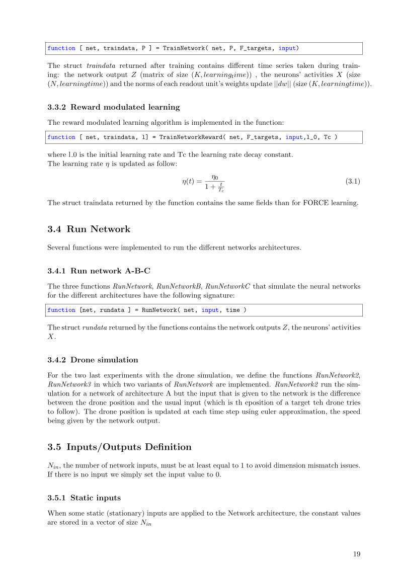
3.3.2 Reward modulated learning

The reward modulated learning algorithm is implemented in the function:

function [ net, traindata, l] = TrainNetworkReward( net, F_targets, input,l_0, Tc )

where l 0 is the initial learning rate and Tc the learning rate decay constant.The learning rate η is updated as follow:

η(t) =η0

1 + tTc

(3.1)

The struct traindata returned by the function contains the same fields than for FORCE learning.

3.4 Run Network

Several functions were implemented to run the different networks architectures.

3.4.1 Run network A-B-C

The three functions RunNetwork, RunNetworkB, RunNetworkC that simulate the neural networksfor the different architectures have the following signature:

function [net, rundata ] = RunNetwork( net, input, time )

The struct rundata returned by the functions contains the network outputs Z, the neurons’ activitiesX.

3.4.2 Drone simulation

For the two last experiments with the drone simulation, we define the functions RunNetwork2,RunNetwork3 in which two variants of RunNetwork are implemented. RunNetwork2 run the sim-ulation for a network of architecture A but the input that is given to the network is the differencebetween the drone position and the usual input (which is th eposition of a target teh drone triesto follow). The drone position is updated at each time step using euler approximation, the speedbeing given by the network output.

3.5 Inputs/Outputs Definition

Nin, the number of network inputs, must be at least equal to 1 to avoid dimension mismatch issues.If there is no input we simply set the input value to 0.

3.5.1 Static inputs

When some static (stationary) inputs are applied to the Network architecture, the constant valuesare stored in a vector of size Nin

19

3.5.2 Dynamic inputs

When the Network is fed with continuous dynamic inputs, the inputs’ continuous values is storedin a matrix of size (Nin, time) where each line correspond to the value of one of the input overtime.

3.5.3 Target functions

The desired outputs that we want the network to produce through the read out units are storedin a matrix of size (K, learningtime) where the ith line correspond to the desired value for the ith

read out unit over the learning time.

20

4 Generating periodic patterns

... etincelle qui fuit !

The first experiments consisted in training the networks with the two algorithms described in 2.2to produce different periodic patterns. In this part we used some networks of architecture A withrespectively 500 and 1000 neurons with FORCE learning and reward modulated learning, and arewiring probability of 0.1 with both algorithms.

4.1 No input

We first consider some neural networks without incoming current. The self-sustained activity isthen due to the recurrent architecture.

4.1.1 Single output

4.1.1.1 Simple sinusoid

We trained the network to produce a simple sinusoid function. The figure 4.1 shows the networkoutput during the training. We can see that it matches perfectly the target from the beginning oflearning. As expected the norm of the weights update decreases over time to stay close to 0 after5 seconds.

21

Figure 4.1: FORCE Learning of a sinusoid pattern

The figure 4.2 shows the network output after learning. Before the simulation the neuron’smembrane potential are reinitialized to random values. The output (in blue) quickly converge tothe desired periodic pattern. The error cannot be easily measured because of the phase differencebetween the real output and the desired target function.

Figure 4.2: Post-learning simulation

22

4.1.1.2 More complex target

The second step consisted in training the network to produce a more complex periodic function.The target function was defined according to one of the experiment in [2].

f(t) = sin(2πt)1.3

1.5+ sin(4πt)

1.3

3+ sin(6πt)

1.3

9+ sin(8πt)

1.3

3; (4.1)

FORCE learningApplying FORCE learning to the match this more complex desired output leads to similar resultsthan with the simple sine wave. The only difference being that it take twice the time (10 seconds)for the weight update to converge to zero as shown on figure 4.3.After the training and the neuron’s potential random reinitialization, the network output convergeto the desired pattern as shown on figure4.4.

Figure 4.3: FORCE learning of a complex periodic pattern

23

Figure 4.4: Post-learning simulation of a network trained with FORCE learning to produce a com-plex pattern

Reward learningWe also tried to apply the reward modulated learning rule to learn the same complex pattern. Thefigure 4.5 shows the output evolution during training. The first two plots represent the outputduring the 5 first and last seconds of learning. We can see that the output progressively followsthe desired target function. The training duration is however longer than with FORCE learning (alearning of at least 100 s was necessary to obtain reasonable results in this case).The figure 4.6 shows the exploration noise which is added to the feedback loop only during training.The network was tested after learning without the neurons’ potentials being reinitialized. In thiscase the network follows the desired pattern but with a slight difference in the signal frequencywhich explains the separation of the two lines that represent the real and the desired outputs infigure 4.7.When we tried the run the network after reinitializing the membranes potential. The network oftenfail to converge to the desired output as shown on figure 4.8 where it converges to a similar butstill different pattern. The figure 4.9 shows the case where the network succeed to converge to thedesired pattern.

24

Figure 4.5: Reward modulated learning of a complex periodic pattern

Figure 4.6: Exploration noise added to the feedback loop during reward modulated learning

25

Figure 4.7: Post-learning simulation of a network trained with reward learning to produce a complexpattern, without reinitialization of the neurons potentials

Figure 4.8: Post-learning simulation of a network trained with reward learning. Convergence failure

Figure 4.9: Post-learning simulation of a network trained with reward learning. Convergence suc-cess

4.1.2 Multiple outputs

The next step of our experiments was to train the network to produce multiple outputs at the sametime with the FORCE learning algorithm, still with no incoming current. Each output is associatedto a different readout unit whose weights are independently updated (they share the same matrixP but different error terms e in the equation 2.5.We trained the network with the two following target functions:

f1(t) = 1.5sin(2πt) (4.2)

f2(t) = 0.7cos(5πt) (4.3)

The figures 4.10 and 4.11 shows the results of the training which are similar to the single outputcase. Both outputs match their target functions during the training and converge quickly to itduring during the simulation.

26

Figure 4.10: FORCE learning of 2 outputs simultaneously

Figure 4.11: Post learning simulation of the 2 outputs network trained with FORCE learning

4.2 Input/output matching

In the last experiment of this chapter we consider a network of 1000 neurons with two read-outunits that receive an incoming current input. We trained the network using FORCE learning inorder to match two different behaviours with two different input values.The input values i1 and i2 are randomly generated in the range [−1, 1]. For the learning to succeedthe two values must however be significantly different. Each input was associated with the twodesired outputs as follow:

when input = i1:

f1(t) = 1.0sin(5

3πt) (4.4)

f2(t) = 0.5cos(5πt) (4.5)

27

when input = i2:

f1(t) = 1.5cos(5

2πt) (4.6)

f2(t) = 0.6sin(5

4πt) (4.7)

We applied the training algorithm once for each input/outputs configuration with a learning timeof 5 seconds.The figures 4.12 to 4.15 shows the results of this experiment.

Figure 4.12: First training (input = i1 = 0.5)

Figure 4.13: Second training (input = i2 = −0.8)

28

Figure 4.14: Post-learning simulation of input/outputs matching (input = i1 = 0.5)

Figure 4.15: Post-learning simulation of input/outputs matching (input = i2 = −0.8)

4.3 Conclusion

This part presented the first replications of the results of [1] in the chronological order of theirimplementation. The most interesting results are the one of the last experiment that a fortioriimply the previous ones. It shows that FORCE learning can be applied to the generation ofmultiple non similar outputs(different frequency and amplitude) and that inputs can be used toswitch between different behaviours.Regarding the reward-modulated learning, although the first results (4.1.1.2) are convincing weencountered some trouble when it came to the multiple output generation. We focus on the followingchapters on FORCE learning algorithms.

29

Regarding the two other network architectures presented in 2.1.2 and 2.1.3, we tried to obtain thesame results as those presented above with more or less success. In those two network configurationsthe training algorithms are really slower than with the architecture A because of the numerousmatrices that need to be updated at each iteration (respectively NG and NF matrices P i forarchitectures B and C). That’s why in the following part we only used the network of architectureA (see Figure 2.1).

30

5 Application to a robot arm

Eclair qui sort de l’ombre ...

5.1 Robot description

In this chapter we consider a robot arm with two joints. Each arm section is defined by itslength (L1, L2) and the first joint is fixed in 2D space in which the robot evolves (the first jointcoordinates are (0, 0)). The degree of freedom of each angle allow the robot to describe a widerange of movements in the 2D space. We name v and w the angles between the two joints and thehorizontal line.The figure 5.1 shows the robot arm with the two angles.The position (x, y) of the robot arm’s end evolve according to the following equation:

x = L1.cos(v) + L2.cos(v + w) (5.1)

y = L1.sin(v) + L2.sin(v + w) (5.2)

To inverse this equation and obtain the angle from the position we use the following equations:

k =x2 + y2 − L12 − L22

2.L1.L2(5.3)

w = atan2(√

1− k2, k) [2π] (5.4)

v = atan2(y, x)− atan2(L1 + L2.cos(w), L2.sin(w)) [2π] (5.5)

In this chapter we consider a neural network of 1000 neurons with 2 readout units. The idea is toassociate each joint angle with one of the network output. By learning periodic patterns we canmake the robot arm describe some periodic movement.

31

Figure 5.1: Robot arm description

5.2 Matching inputs with different movements

In the first experiment we train the network to produce 3 pairs of outputs depending on one inputthat take 3 different values (i1,i2,i3) that are randomly generated in the range ([−1, 1]). Thisexperiment is similar to the one in 4.2, except that we learn 3 pairs of output instead of two, andthat the target functions are more complex.The 3 pairs of outputs that are trained correspond to 3 trajectory: a square, a circle and a loopof different amplitude and centred on the same point. The target functions are obtained from thedesired trajectory with equations 5.3 and 5.5. After the simulation, the trajectory that is effectivelyfollowed by the arm is obtained from the network outputs with equations 5.1 and 5.2.The figures 5.2 to 5.4 show the training data, and the figures 5.5 to 5.7 show the results of thesimulation after the training. Figure 5.8 shows the actual trajectory during the post-learningsimulation. We can see that when the input changes (different color on the figure) the robotconverge to the desired movement that it then repeated until the input changes again. By usinga different number of neurons we can get more precise result but the learning will be longer. Forexample it is possible to improve the square trajectory,especially at the corners.

32

Figure 5.2: FORCE learning of joint angles v and w to produce a squared movement

Figure 5.3: FORCE learning of joint angles v and w to produce a circular movement

33

Figure 5.4: FORCE learning of joint angles v and w to produce a loop movement

Figure 5.5: Post learning simulation (input = i1 = −0.5)

34

Figure 5.6: Post learning simulation (input = i2 = 0.6)

Figure 5.7: Post learning simulation (input = i3 = 0.2)

35

Figure 5.8: Robot arm trajectory during the simulation

5.3 Inputs interpolation to produce new movements

In the second experiment, we focused on one shape and trained the network to produce circles ofdifferent amplitudes depending on the input. In this case we trained the network with 4 values thatwere linearly spaced and no longer randomly generated. During training, the inputs were associatedwith the desired amplitudes that were also linearly spaced. By doing this we managed to producenew desired movements that hadn’t been taught during training by running the network with newinputs whose value were between the values used during training. It shows that the network learnsto produce a circle whose radius is proportionate to the input.To make things clearer the table 5.1 presents the input values that were used during training andsimulation and the associated desired radius. The first 4 values correspond to the one that are usedduring the training where the desired radius is known via the provided target functions. The lastthree values are the one used during the simulation. In the last three cases the associated radius isthe radius that we expect to obtain but is unknown to the network.

Input -0.3 -0.1 0.1 0.3 -0.2 0 0.2

Radius 0.2 0.4 0.6 0.8 0.3 0.5 0.7

Table 5.1: Input and associated circle radius

36

The figure 5.9 shows the result of the simulation. The circles in blue were learned during training.On the contrary the three others circles are produced when the network is run with a new inputvalue. In these cases the new circles are still proportionate to the input. The figure 5.10 showsonly these new circles with the expected radius (in blue).

Figure 5.9: Interpolation to produce new circles

37

Figure 5.10: Producing new circles with the radius depending on the input

After obtaining these results we tried to reproduce the experiment with a different (more complex)shape. The table 5.2 similarly shows the inputs that were used with the associated/expected squareside lengths. The figure 5.11 shows the shapes that are obtained against the expected one (in blue).Although the results are not as accurate as with the simple circular movement, the network stillsucceed in producing a new movement close to the expected one when run with a new input.

Input -0.3 -0.1 0.1 0.3 -0.2 0 0.2

Side length 0.2 0.3 0.4 0.5 0.25 0.35 0.45

Table 5.2: Input and associated square side length

38

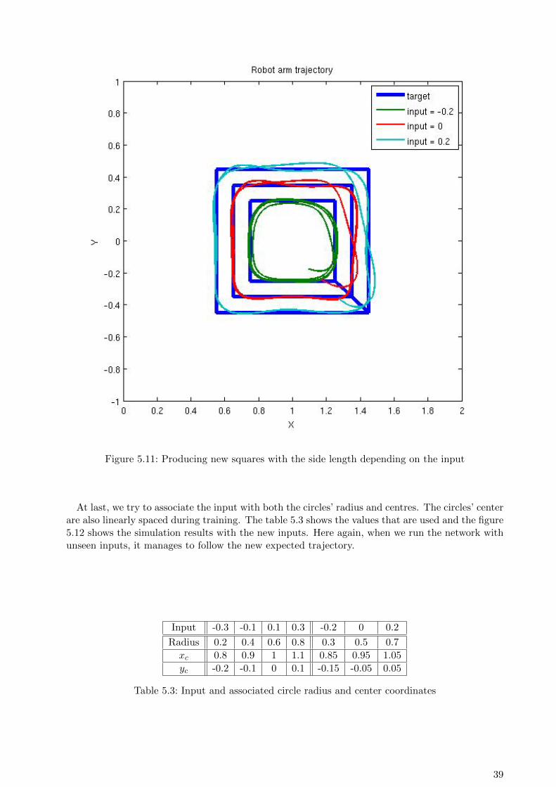
Figure 5.11: Producing new squares with the side length depending on the input

At last, we try to associate the input with both the circles’ radius and centres. The circles’ centerare also linearly spaced during training. The table 5.3 shows the values that are used and the figure5.12 shows the simulation results with the new inputs. Here again, when we run the network withunseen inputs, it manages to follow the new expected trajectory.

Input -0.3 -0.1 0.1 0.3 -0.2 0 0.2

Radius 0.2 0.4 0.6 0.8 0.3 0.5 0.7

xc 0.8 0.9 1 1.1 0.85 0.95 1.05

yc -0.2 -0.1 0 0.1 -0.15 -0.05 0.05

Table 5.3: Input and associated circle radius and center coordinates

39

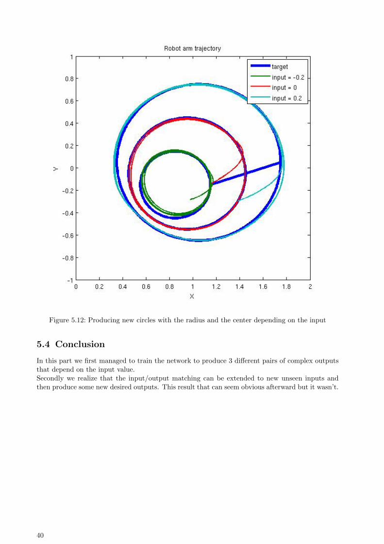
Figure 5.12: Producing new circles with the radius and the center depending on the input

5.4 Conclusion

In this part we first managed to train the network to produce 3 different pairs of complex outputsthat depend on the input value.Secondly we realize that the input/output matching can be extended to new unseen inputs andthen produce some new desired outputs. This result that can seem obvious afterward but it wasn’t.

40

6 Working Memory

... et rentre dans la nuit,

Until now, the network have been used to generate periodic outputs that are analogous to motoroutputs. In this chapter we generate a more complex pattern where the network produces twooutputs, each of them being associated with two inputs. By doing this we manage to generate a2-bits memory: each output keeps record of which one of its two associated inputs had the latestpulsation.

6.1 Input/Output Generation

The inputs are held to zero and at each time step (ie every milisecond) a pulsation of 100 ms occurswith a probability of 0.0005. We first create the binary inputs and for each pair of input we createthe associated binary target function. The binary target switches to 1 when a pulse occurs on itsfirst input, called the ON input, and to -1 when a pulse occur on its second input called the OFFinput. We then use the Matlab function filter with different parameters to transform the binaryinputs and targets into continuous valued functions.The figure 6.1 shows two inputs with their associated output after filtering.

To generate the inputs

Figure 6.1: Inputs/output generation

6.2 Results

After having generated two pairs of inputs values and two associated target functions of length100000 ms as described above, we train the network with these data. The figure 6.2 shows the

41

training results.We then generate 4 new inputs with the same random process and run the neural network withthese new inputs. The figure 6.3 shows the result of this simulation. We can see that each outputis associated with two inputs and switches between 1 and -1 when a pulsation occurs respectivelyon the first (in blue) or the second (in green) input. For more clearness we also plot in red thetarget function corresponding to each pairs of input during the simulation although they are notused in the algorithm. This task is memory-dependent because the network needs to reminds therecent input history.

Figure 6.2: 100 s working memory training

42

Figure 6.3: Working-memory post-learning simulation

6.3 Conclusion

We can also see that the outputs are robust to input noise because one output is only affected bythe two outputs it is associated with, despite the random recurrent connexions of the network.Generating a working memory, even a small and simple one, is a point of great interest becausemany cognitive abilities in the brain require a working memory and the way this process is achievedin the brained has not been completely understood yet.This shows that the networks can learn autonomously a computational rule and develop the requiredworking memory to hold information on its recent input history.

43

7 Application to a Drone controller

Minute que le temps ...

In this last chapter we tried to apply some results of the previous chapters to produce outputsthat could be used as control signals for a drone to follow a target. We reduced our problem to aone dimension problem. The idea would be for the drone to move on the left-right axis in order tocome in front of target. We only simulated the drone trajectory on Matlab, but we had in mind toapply our results to a real ARDrone2.0. This drone is equipped with a frontal camera who couldbe used to detect the target position. We experimented two different approaches that are presentedin the two following sections.

7.1 Following a slow target

Our first approach was to produce an output that would make the drone follow a target which isslowly moving by producing a speed which is directly proportionate to the distance between thedrone and the target. To do so we train the network to produce an output which is equal to theinput with 4 linearly spaced inputs in the range [−1, 1] as seen on figure 7.1. Then when we runthe network with any new input in the same range, it will produce an output equal to the input.Starting from that we can run the network with the input being the difference between the targetposition and the drone position at each time step. The output will be equal to this difference. Thedrone position is updated at each time step using Euler approximation with the network outputbeing used as the speed, i.e. the derivative of the position. The three plots of figure 7.2 shows theresult of the simulation. The first plot shows the target position (in green) and the drone position(in blue) over time. We can see that the two positions stay really close to each other. The secondplot shows the absolute difference between the two positions. The third plot shows the networkoutput (in green) and the derivative of the target position (in blue).

44

Figure 7.1: Post learning simulation

45

Figure 7.2: FORCE learning application to track a moving target

7.2 Following fast target

Our second approach consisted in learning some more complex control signals to make the dronereach a target as quick as possible. Whereas in the first approach, the drone is initially close tothe target and follows it as it moves slowly, in this case the target directly appears at a certaindistance and the drone try to reach it quickly.

7.2.1 input/ouput generation

Every 1500 ms the input which represents the target position changes its value which is randomlygenerated in the range [-2.5:0.25:2.5]. We try to define empirically what seems to be the optimaltrajectory to reach this point. To produce the trajectory we use the following equation which isthe solution of a second order differential equations with constant coefficients:

trajectory(d, c, T ) = c+(d−c)(1−e−ζ.ω0.T .cos(ω0.√

1− ζ2.T )− ζ√1− z2

.e−ζ.ω0.T .sin(ω0.√

1− ζ2.T ))

(7.1)where

• ζ is the system damping coefficient (ζ > 0)

• ω0 is the system natural frequency

• d is the desired position

• c is the current position

46

To generate the control signal associated with the input, we differentiate the desired continuoustrajectory that we obtained from the inputs. The figures 7.3 and 7.4 shows the results of the processwith different damping coefficients values. On each figure the first plot shows the input (in blue),i.e. the target position, and the associated trajectory to reach this position (in green). The secondplot shows the derivative of the trajectory that we want the neural network to generate.

Figure 7.3: Input and corresponding desired output (damping coefficient ζ = 0.2)

47

Figure 7.4: Input and corresponding desired output (damping coefficient ζ = 09)

7.2.2 Learning the aperiodic control signal

After having generated some 100000 ms long time series of inputs and the associated outputs, wetrain the network with these data. The figure 7.5 shows the training results.

48

Figure 7.5: 25 s of FORCE learning of the drone control signal

We then generate a new time series of inputs, which is now taken in the range [−2.5 : 1.667 : 2.5]i.e. the difference between the input value at different times is a multiple of 0.1667 instead of 0.25like in the training. We also generate the smooth trajectory and the control signal associated withthe new input. When the network is run with this new input time series it produces the expectedcontrol signal as seen on figures 7.6 and 7.7. On these figures, the first plot shows the desiredoutput and the one produced by the network which are almost the same (the second plot showsthe absolute difference between the actual and the expected control signal). The third plot showsthe input with the step size every time the input changes. The fourth plot shows the trajectoryobtained by integrating the network output, together with the desired trajectory.Because we sum up the control signal to obtain the trajectory, the error also sums up over timewhich explains the deviation from the expected trajectory. However in practice the deviation fromthe desired trajectory would induce a change in the input which represents the distance betweenour drone and the target, so the error would be corrected over time.These results are very interesting for two reasons.First, we manage to produce a signal that does not depend on the input absolute value but on itsrelative value. The control signal amplitude is proportionate to the size of the difference in theinput value.

49

The second interesting results is that the network can be run with new input values (more preciselywith new input step size), that haven’t been seen during training. In this case the network stillproduce the correct control signal that it hadn’t been trained to generate.

Figure 7.6: Network simulation on unseen input values (the desired trajectory and the associatedcontrol signal are produced with a damping coefficient ζ = 0.5)

50

Figure 7.7: Network simulation on unseen input values (the desired trajectory and the associatedcontrol signal are produced with a damping coefficient ζ = 0.9)

7.3 Conclusion

In this part we managed to extend the result we found in a part 5.3 where we managed to produce acircle of any radius by simply learning to produce 4 different circles. Here we learn a small repertoireof aperiodic control signals but managed to produce a wide range of different signals by using newinputs after the learning. This phenomena is really interesting and even if we had the intuitionit might happen it wasn’t guarantee at all. To our knowledge, this kind of input interpolation to

51

produce new outputs with reservoir computing hasn’t been done before and it might be interestingto test it further or to think of other applications.Regarding the drone control itself, the next chapter describes what could be the future steps toreach our goal.

52

8 Future perspectives

... prete et retire a l’homme.

Lamartine

8.1 Collecting real training data

In section 7.2 of the last chapter we assumed that the best strategy to quickly reach a target wasto reach it with a high speed, even if that means going a little too far and then going back a bit. Amore relevant approach would consist in collecting real data on the drone to use a more accuratecontrol signal.An expert could pilot the real drone and reach some points at different distances as quick as possible.We tried to run such an experiment with an ARDrone but the results were not convincing becausethe data we collected were very noisy. However the experiment could be run again in a betterenvironment and hopefully provide some data that could be used to train the neural network.An other solution to collect training data would be to use a proper drone simulator.

8.2 Further training

In the last chapter, we train the network to produce the desired speed to apply to the drone. How-ever, although the drone has a high acceleration, the control signal to apply to the Drone mightnot be exactly equal or proportionate to the desired speed because of the drone inertia. A futurething to be done would be to explore other shapes of control signals to apply to the drone to obtainthe desired speed and trajectory.We limited our study on the drone to a one dimension movement. A following step would be toextend our results to several dimensions. We could have two inputs, each controlling the dronetrajectory on one dimension. As we saw in chapter 6 where we implemented a working memory, itis possible to make an input having an effect on one output without affecting the others outputs.However some problem occur when we want the input to evolve in a wide range of continuousand previously unseen values like it was the case for the drone. In this case when an input takea different value, the network might not be able to know which input has changed. Moreover ifseveral inputs changes at the same time, each neuron receive the weighted sum of the inputs (Nin∑j=1

JGInij Ij(t)) it can not know which input as changed and of how much.

We could also imagine training the network to produce a large repertoire of behaviour and move-ment and then use some properly speaking reinforcement learning techniques to teach the dronehow to use a combination of these different behaviour to reach any point.

53

Conclusion

The first parts of this project confirmed the results of some experiments that had alreadybeen made. Reproducing these results from scratch was a really good way to get familiar with thelearning algorithms and the use of recurrent neural networks before going further. We managedto generate several complex periodic patterns and to realize some inputs/outputs matching ina wide range of frequencies. We also reproduced a two-bits working memory which is a complexcomputational structure. Being able to train a chaotic recurrent network to generate this behaviourcan shed a new light on how such operations are achieved in the brain which is still an area ofresearch.

However the main interest of this project is the new kind of training we realized and that, asfar as we know, hadn’t been done before. By training the network with only four different inputvalues, we can produce a complex periodic output that will be proportionate to any new inputtaken in the range of the inputs used during training. For example, in our case, we managed toproduce a circle of any radius in a certain range whereas only four circles had been learned duringtraining. This is quite challenging because usually the input that were used during training werethe same that were used during the simulation. It wasn’t obvious at all that such an interpolationwould succeed and that we would be able to generate new correct outputs by using intermediateinput values. The extension of these results to the generation of more complex aperiodic patternsis also very promising. Although we are not sure whether this could be used to completely pilot adrone, this question deserve to be investigated. Moreover there might other areas were this kind oflearning could be very useful.

To conclude this project was an amazing opportunity to become more familiar with the veryinteresting field of recurrent neural network. It was interesting and challenging to be free to exploredifferent applications of such networks to finally arrive to a more precise goal step by step.

54

Bibliography

[1] D. Sussillo and L.F. Abbott - Generating coherent patterns of activity from chaotic neuralnetworks. 2009

[2] G.M. Hoerzer, R. Legenstein and W. Maas - Emergence of Complex Computational StructuresFrom Chaotic Neural Networks Through Reward-Modulated Hebbian Learning. 2012

[3] Hopfield - Neurons with graded response have collective computational properties like those oftwo-states neurons. 1984

[4] Haykin - Neural networks: a comprehensive foundation. 1999

[5] Beer - On the dynamics of small continuous-time recurrent neural networks. 1995

[6] Sompolinsky, Crisanti and Sommers - Chaos in random neural networks. 1988

[7] Bertschinger and Natschlger - Real-time computation at the edge of chaos in recurrent neuralnetworks. 2004

[8] http://reservoir-computing.org/.

[9] H. Jaeger - The ”echo state” approach to analysing and training recurrent neural networks -with an Erratum note. 2001

[10] T. Natschlager, W. Maass, and H. Markram - The ”Liquid Computer”: A Novel Strategy forReal-Time Computing on Time Series. 2002

[11] Nudo et al. - Use-dependent alterations of movement representations in primary motor cortexof adult squirrel monkeys. 1996

[12] Rainer and Miller - Effects of visual experience on the representation of objects in the prefrontalcortex. 2000

[13] Recanzone et al. - Topographic reorganization of the hand representation in cortical area 3bof owl monkeys trained in a frequency-discrimination task. 1992

[14] Klingberg, Forssberg, Westerberg - Training plasticity of working memory in children withADHD. 2002

[15] Klingberg - Training plasticity of working memory. 2010

[16] Legenstein, CHase, Schwartz, Maas - A reward-modulated Hebbian learning rule can explainexperimentally observed network reorganization in a brain control task. 2010

[17] Fremaux, Sprekeler, Gerstner - Functional Requirements for Reward-Modulated Spike-Timing-Dependent Plasticity. 2010

[18] Fiete, Seung - Gradient Learning in Spiking Neural Networks by Dynamic Perturbation ofConductances. 2006

[19] Sussillo - Learning in chaotic recurrent networks. 2009

55