CHAOTIC HOPPING BETWEEN

ATTRACTORS IN NEURAL NETWORKS

Joaquın Marro, Joaquın J. Torres∗, and Jesus M. Cortes†

Institute Carlos I for Theoretical and Computational Physics, andDepartamento de Electromagnetismo y Fısica de la Materia,

University of Granada, E-18071–Granada, Spain.

∗Corresponding author: Joaquın J. Torres, Department of Electromagnetism andPhysics of the Matter, University of Granada, E-18071 Granada Spain; Tlf: (+34)958244014; Fax: (+34) 95824 23 53 email: jtorres@onsager.ugr.es

†Present address: Institute for Adaptive and Neural Computation, School of Informat-ics, The University of Edinburgh, 5 Forrest Hill, Edinburgh EH1 2QL, Scotland UK

1

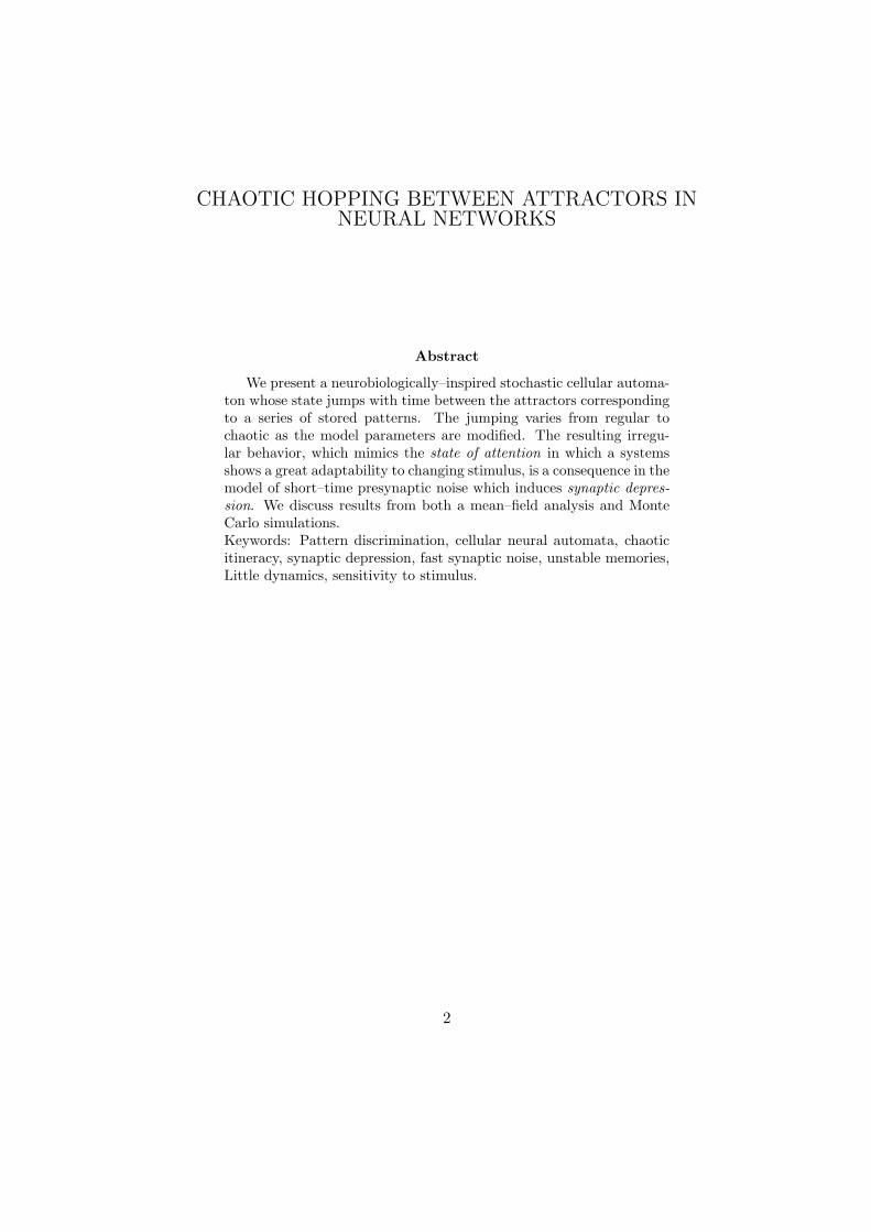
CHAOTIC HOPPING BETWEEN ATTRACTORS INNEURAL NETWORKS

Abstract

We present a neurobiologically–inspired stochastic cellular automa-ton whose state jumps with time between the attractors correspondingto a series of stored patterns. The jumping varies from regular tochaotic as the model parameters are modified. The resulting irregu-lar behavior, which mimics the state of attention in which a systemsshows a great adaptability to changing stimulus, is a consequence in themodel of short–time presynaptic noise which induces synaptic depres-sion. We discuss results from both a mean–field analysis and MonteCarlo simulations.Keywords: Pattern discrimination, cellular neural automata, chaoticitineracy, synaptic depression, fast synaptic noise, unstable memories,Little dynamics, sensitivity to stimulus.

2

1 Introduction

Analysis of electroencephalogram time series, though perhaps not conclusiveyet, suggest that some of the brain high level tasks might require chaoticactivity and itinerancy (Barrie et al., 1996; Tsuda, 2001; Korn and Faure,2003; Freeman, 2003). As a matter of fact, following the observation of con-structive chaos in many natural systems (Kiel and Elliot, 1996; Kaneko andTsuda, 2001; Strogatz, 2003), it has been reported some evidence of sensi-tivity enhancement associated to a critical state of synchronization duringexpectation and attention (Hansel and Sompolinsky, 1996), and it has beenargued that chaos might provide an efficient means to discriminate different(e.g.) olfactory stimuli (Ashwin and Timme, 2005) for example. Conse-quently, there has recently been some effort in incorporating constructivechaos in neural network modeling (Wang et al., 1990; Bolle and Vink, 1996;Dominguez and Theumann, 1997; Caroppo et al., 1999; Poon and Bara-hona, 2001; Mainieri and Jr., 2002; Katayama et al., 2003). Concludingon the significance of chaos in neurobiological systems is still an open issue(Rabinovich and Abarbanel, 1998; Faure and Korn, 2001; Korn and Faure,2003), however.

As a new effort towards better understanding this issue, in the presentpaper we present, and study both analytically and numerically, a neuralautomaton which exhibits chaotic behavior. More specifically, it shows sortof dynamic associative memory, consisting of chaotic hopping between thestored memories, which mimics the brain states of attention and searching.The model is a cellular automaton, in which dynamics concerns the whole,which is simultaneously updated —instead of sequentially updating a smallneighborhood at each time step. This automaton (or Little dynamics) strat-egy has already revealed efficient in modeling several aspects of associativememory (Ganguly et al., 2003; Cortes et al., 2004). Interesting enough, itis a fact that, concerning this property, neural automata often exhibit moreinteresting behavior than their Hopfield–like, sequentially–updated counter-parts in which any two successive states are stronger correlated. Therefore,we extend in this paper to cellular automata our recent study of the effectsof synaptic “noise” on the stability of attractors in Hopfield–like networks(Cortes et al., 2006). That is, we present here a detailed study of cellu-lar automata in which a certain type of neurobiologically–inspired synapticfluctuations determine an interesting retrieval process. Our model synap-tic fluctuations are coupled to the presynaptic activity in such a way thatsynaptic depression occurs. This phenomenon, which has been observed inactual systems, consists in a lowering of the neurotransmitters release after

3

a period of intense presynaptic activity (Tsodyks et al., 1998; Pantic et al.,2002). Our model fluctuations happen to destabilize the memory attractorsand are shown to induce, eventually, regular and even chaotic dynamics be-tween the stored patterns. Confirming expectations mentioned above, wealso show that our model behavior implies a high adaptability to a changingenvironment, which seems to be one of the nature strategies for efficientcomputation (Lu et al., 2003; Schweighofer et al., 2004).

2 The model

Let a set of N binary neurons, S =si = ±1; i = 1, . . . , N, connected bysynapses of intensity:

wij = wLijxj , ∀i, j. (1)

Here, xj ∈ R stands for a random variable, and wLij is an average weight.

The specific choice for the latter is not essential here but, for simplicity andreference purposes, we shall consider a Hebbian learning rule (Amit, 1989).That is, we shall assume in the following that synapses store a set of Mbinary patterns, ξµ = ξµ

i = ±1; i = 1, . . . , N , µ = 1, ..., M, according tothe prescription, wL

ij = M−1∑

µ ξµi ξµ

j . The stored patterns are assumed to berandom, i.e., p (ξµ

i ) = 12δ (ξµ

i − 1) + 12δ (ξµ

i + 1) , unless otherwise indicated.Notice that our restriction to binary neurons is neither essentially; in fact, itwas shown (Pantic et al., 2002) that the behavior of binary networks agreesqualitatively with the behavior observed in more realistic networks including,for instance, integrate and fire neuron models. However, consistent withthe choice of a binary code for the neurons activity, we are assuming zerothresholds, θi = 0, ∀i, in the following; this is relevant when comparing thiswork with some related one, as discussed below.

The set X =xj of random variables is intended to model some reportedfluctuations of the synaptic weights. To be more specific, the multiplicativenoise in (1), which was recently used to implement a variation of the Hop-field model (Cortes et al., 2006), may have different competing causes inpractice, ranging from short–length stochasticities, e.g., those associatedwith the opening and closing of the vesicles and with local variations in theneurotransmitters concentration, to time lags in the incoming long–lengthsignals (Franks et al., 2003). These effects will result in short–time, i.e.,relatively fast microscopic noise. As a matter of fact, the typical synapticvariability is reported to occur on a time scale which is small compared withthe characteristic system relaxation (Zador, 1998). Therefore, as far as Xcorresponds to microscopic fast noise, neurons will evolve as in presence of

4

a steady distribution, say P st(X|S). It follows that such noise will modifythe local fields, hi(S,X) =

∑j 6=i wijxjsj , i.e., the total presynaptic current

which arrives to the postsynaptic neuron si, which one may assume to begiven in practice by

hi(S) =∫

Xhi(S,X)P st(X|S)dX. (2)

This, which is a main feature of our automaton, amounts to assume thateach neuron endures an effective field which is, in fact, the average contri-bution of all possible different realizations of the actual field (Bibitchkovet al., 2002). This situation corresponds to the familiar adiabatic elimina-tion of fast variables which is discussed in many books, e.g., in (Marro andDickman, 1999).

Next, one needs to model the noise steady distribution. Motivated bysome recent neurobiological findings, we would like this to mimic short–term synaptic depression (Tsodyks et al., 1998; Pantic et al., 2002). Thisrefers to the observation that the synaptic weight decreases under repeatedpresynaptic activation. The question is how such mechanism may affect theautomata (and, in turn, actual systems) dynamics. For simplicity, we shallassume factorization of the noise distribution, i.e., we assume the simplestcase P st(X|S) =

∏j P (xj |S), and the distribution of the stochastic variable

in (1) is

P (xj |S) = ζ (~m) δ(xj + Φ) + [1− ζ (~m)] δ(xj − 1). (3)

Here, ~m = ~m(S) stands for the overlap vector of components mµ(S) =N−1

∑i ξ

µi si, and ζ (~m) is an increasing function of ~m to be determined.

The choice (3) amounts to assume that, with probability ζ (~m) , i.e., morelikely the larger ~m is, which implies a larger net current arriving to thepostsynaptic neurons, the synaptic weight will be depressed by a factor −Φ.Otherwise, the weight is given the chosen average value, see equation (1).Interesting enough, (3) clearly induces some non–trivial correlations betweensynaptic noise and neural activity. This is an additional bonus of our choice,as it conforms the general expectation that processing of information in anetwork will depend on the noise affecting the communication lines andvice versa. Looking for an increasing function of the total presynaptic cur-rent with proper normalization, a simple choice for the probability in (3)is ζ (~m) = (1 + α)−1 ∑

µ [mµ (S)]2 , where α = M/N is the load parame-ter or network capacity. It then follows after some simple algebra that the

5

resulting fields are

hi(S) =

1− γ

∑µ

[mµ (S)]2∑

ν

ξνi mν (S) , (4)

where γ ≡ (1 + Φ) (1 + α)−1 . Notice that this precisely reduces for Φ →−1 to the local fields in the Hopfield model in which the synaptic weightsdo not fluctuate but are constant in time (Amit, 1989). Otherwise, thisamounts to modulate the Hebb prescrition with a mean effect, namely, 1−γ

∑µ [mµ (S)]2 , which accounts for the average of many depressing synapses

connected to each other. This is precisely equivalent to the (mean–field)depressing effect in a recurrent network (Tsodyks et al., 1998; Pantic et al.,2002).

Time evolution is due to competition between the fields (4), which con-tain the effects of synaptic noise, and some additional natural stochasticityof the neural activity. In accordance with a familiar hypothesis, we shall as-sume this stochasticity controlled by a “temperature” parameter, T, whichcharacterizes an underlying “thermal bath” (Marro and Dickman, 1999).Consequently, evolution is by the stochastic equation

Πt+1(S) =∑

S′Πt(S′)Ω(S′ → S), (5)

where the probability of a transition is (see, for instance (Coolen, 2001):

Ω(S′ → S) =N∏

i=1

ω(s′i → si). (6)

For simplicity and concreteness, we take ω(s′i → si) ∝ Ψ [βi (s′i − si)] ,where βi ≡ T−1hi(S′), and hi(S′) independent of s′i, which is a good ap-proximation for a sufficiently large network (technically, this is an exactproperty in the thermodynamic limit N → ∞). The function Ψ is arbi-trary except that, in order to obtain well defined limits, we require thatΨ(u) = Ψ(−u) exp(u), Ψ(0) = 1 and Ψ(∞) = 0, which holds for a nor-malized exponential function (Marro and Dickman, 1999). Then, consistentwith the condition

∑S Ω(S′ → S) = 1, we take

ω(s′i → si) = Ψ[βi(s′i − si)][1 + Ψ

(2βis

′i

)]−1. (7)

6

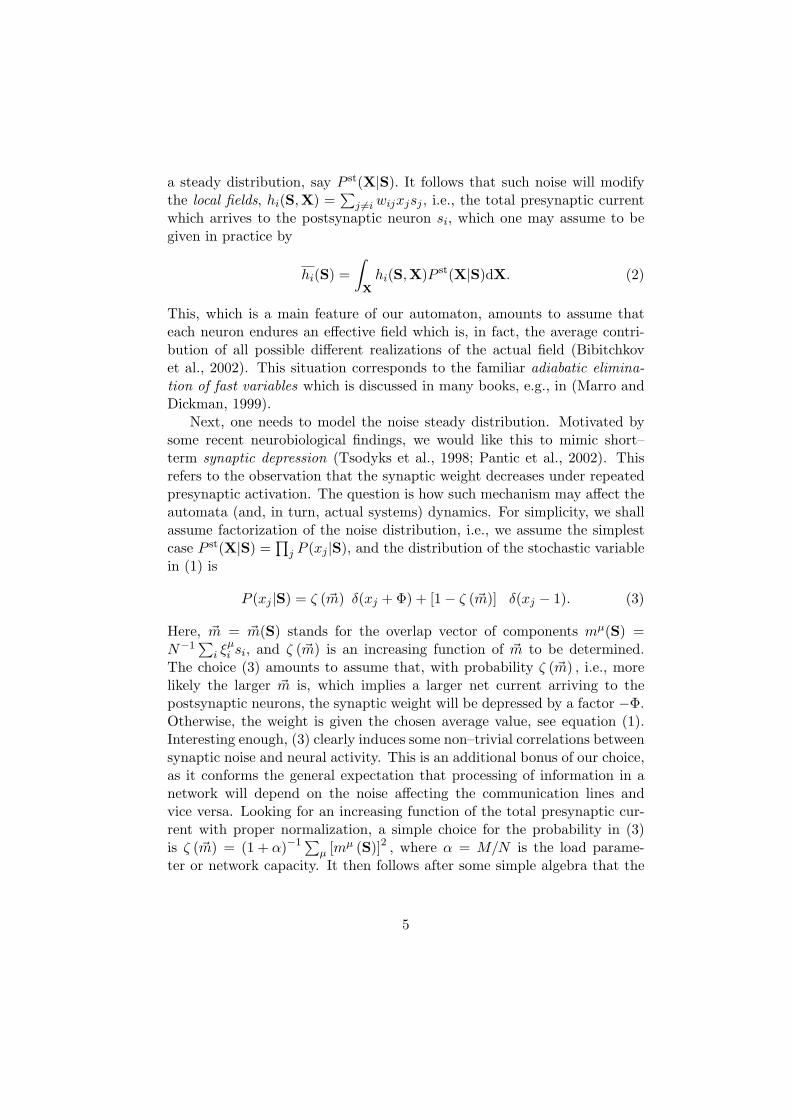
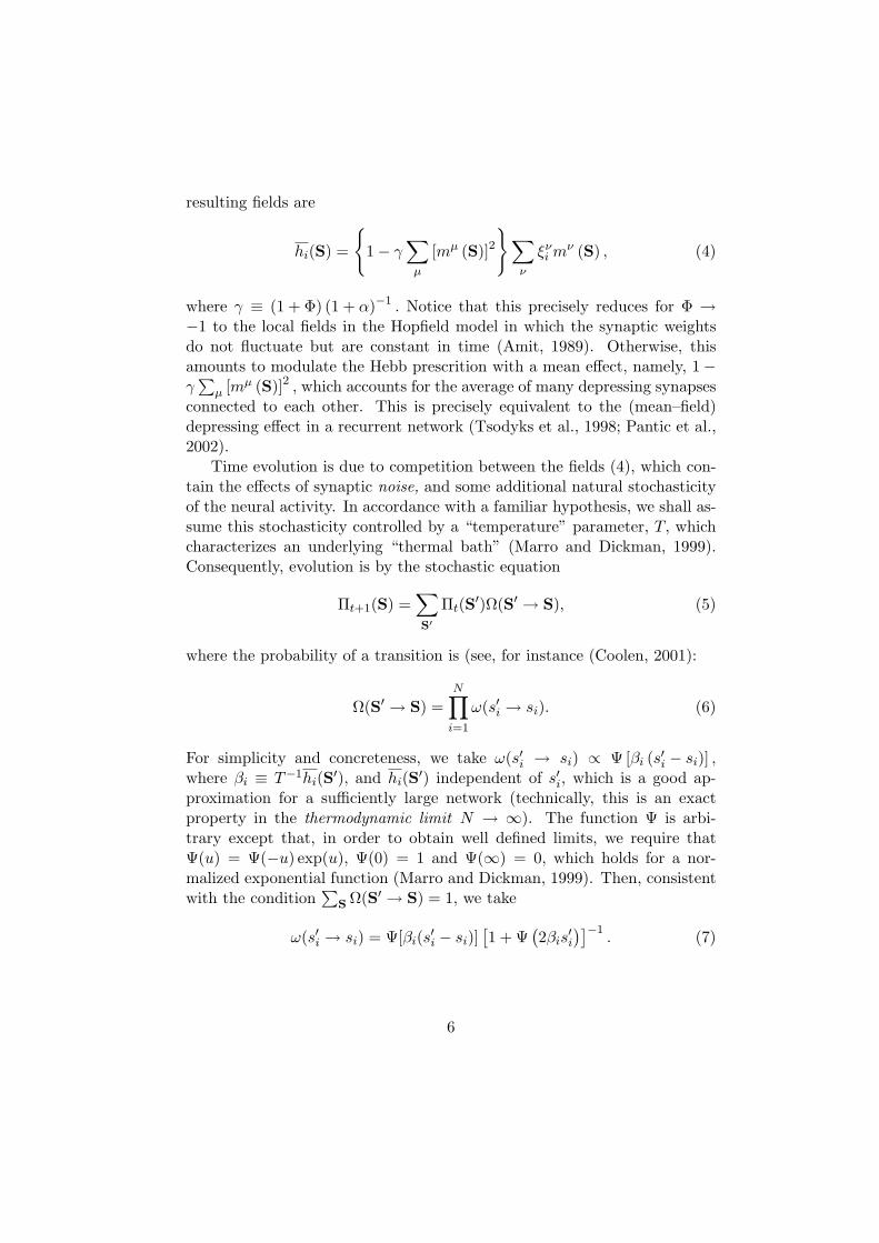
3 Main results

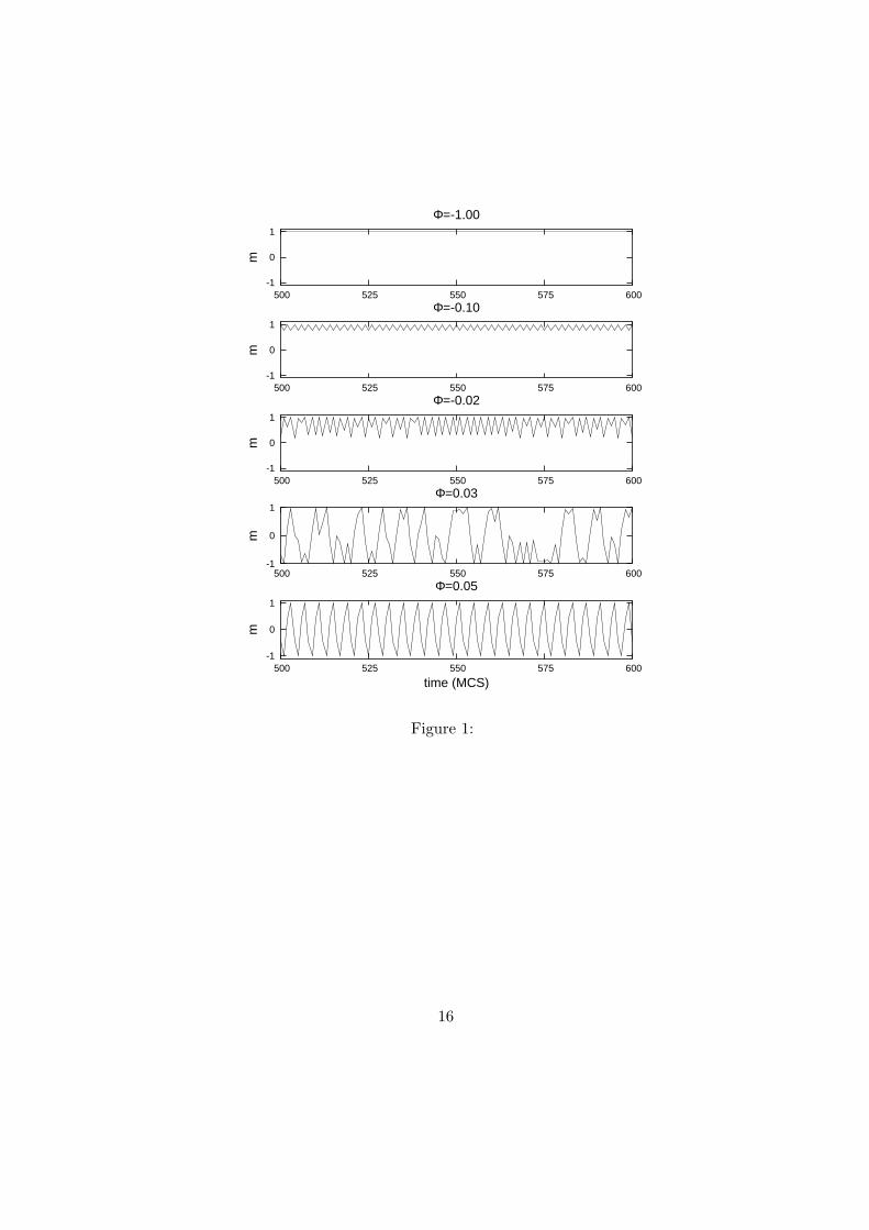
It is obvious that the above may be adapted to cover other, more involvedcases, but model (4)-(7) is enough to our purposes here. In fact, MonteCarlo simulations of this case reveal some new interesting facts as comparedwith the case of sequential updating in (Cortes et al., 2006). To beginwith, figure 1 illustrates a much varied landscape, namely, the occurrence offixed points, cycles, regular and irregular hopping between the attractors.This may also be obtained analytically under the mean–field assumptionthat si = 〈si〉 ∀i (Amit, 1989) which holds for a fully connected network.Following the standard procedure (Coolen 2001), we obtain from (4)-(7) forM = 1 a discrete map which describes time evolution of the overlap m ≡ m1

asmt+1 = tanhT−1mt[1−m2

t (1 + Φ)]. (8)

Notice that no real approximation is involved in this derivation, but it con-cerns a recurrent, fully connected network. As one varies in (8) the “tem-perature” T and the depressing parameter Φ, it follows a varying situationin perfect agreement with the Monte Carlo simulations, as expected. Inparticular, figure 2 shows the occurrence of chaos in a case in which thermalfluctuations are small compared to the synaptic noise. That is, the Lya-punov exponent, λ, corresponding to the dynamic mean–field map showsdifferent chaotic windows, i.e., λ > 0, as one varies Φ for a fixed T. As illus-trated also in figure 2, dynamics is stable for Φ = −1, i.e., in the absenceof any synaptic noise, and the only solutions then correspond to the onesthat characterize the familiar Hopfield case with parallel updating. As Φ isincreased, however, the system tends to become unstable, and transitionsbetween m = 1 and m = −1 then eventually occur that are fully chaotic.This behaviour can be easily understood by studying local stability of thesolutions of the map (8). This requires |λ| < 1 with λ ≡ ∂F (m,T,Φ)

∂m |m=m∗ ,where F (m,T,Φ) ≡ tanhT−1mt[1−m2

t (1+Φ)] and m∗ is the steady statesolution (for t →∞) of the map (8). The critical condition λ = 1 marks theappearance of locally stable non-trivial solutions (m∗ 6= 0) in a steady-statebifurcation, which is supercritical for T < Tc = 1 and Φ > Φc = −4

3 andsubcritical for Φ < Φc = −4

3 . In the latter case, locally stable solutions show

sharply at temperature T > Tc, with overlaps such that |m∗| > 1√3

(Tc−TΦ−Φc

) 12

(Cortes et al., 2006). On the other hand, the other critical condition for localstability, namely λ = −1, marks the existence of a period-doubling bifur-cation driving the system to a chaotic regime, as shown in figure 2. This

7

occurs at given temperature T for Φ > Φpd = 13(m∗)2

(1 + T

1−(m∗)2

)− 1,

which is Φpd ≈ −0.17 for T = 0.1 and m∗ ≈ 0.96 as in figure 2.There is also chaotic hopping between the attractors when the system

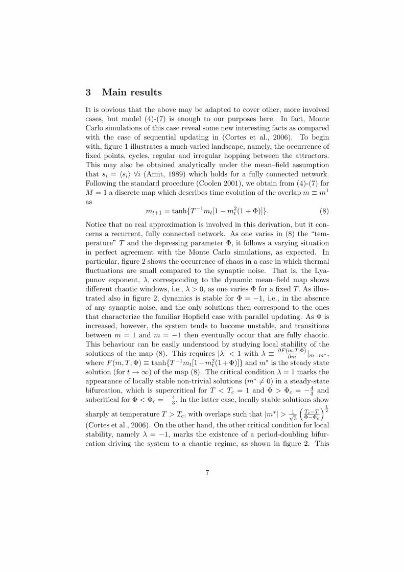
stores several patterns, i.e., for M > 1. In this case, we obtain the morecomplex, multidimensional map:

mν(S)(t + 1) =1N

∑

i

ξνi tanh[βhi(S)(t)] ∀ν = 1, . . .M. (9)

This is to be numerically iterated. The simplest order parameter to monitorthis is:

ζ =1

1 + α

∑µ

(mµ(S))2 . (10)

This is shown in figure 3 as a function of Φ. The graph clearly illustrates aregion of irregular behavior which has a width ∆Φc defined as the distance,in terms of Φ, from the first bifurcation to the last one. Interesting enough,we find that the width of this region is practically independent of the numberof patterns; that is, we find that ∆Φc = 0.575± 0.005 as M is varied withinthe range M ∈ [1, 50] . This suggests that the chaotic behavior which occursfor depressing fast synaptic fluctuations, i.e., for any Φ > −1, does notcritically depend on the automaton capacity but the model properties arerather robust and perhaps independent of the number of stored patternswithin a wide range. One may expect, however, that some of the interestingmodel properties will tend to wash out as the load parameter increasesmacroscopically, i.e., as M →∞.

4 Discussion and further results

Motivated by the fact that analysis of brain waves provides some indica-tion that the chaos–theory concept of strange attractor could be relevant todescribe some of the neural activity, we presented here a neurobiologically–inspired model which exhibits chaotic behavior. The model is a (micro-scopic) cellular automaton with only two parameters, T and Φ, which con-trol the thermal stochasticity of the neural activity and the depressing effectof (coupled) fast synaptic fluctuations, respectively. Our system reduces tothe Hopfield case with Little dynamics (parallel updating) only for Φ = −1.

Our main result is that, as described in detail in the previous section,the automaton eventually exhibits chaotic behavior for Φ 6= −1, but not forΦ = −1, nor in the case of sequential, single–neuron updating irrespective of

8

the value of Φ (Cortes et al., 2006). It also follows from our analysis abovethat further study of this system and related automata is needed in orderto determine other conditions for chaotic hopping. For example, one wouldlike to know if synchronization of all variables is required, and the precisemechanism for moving from regular to irregular behavior as Φ is slightlymodified. We are pursuing the present effort along this line, and will planto present soon some related preliminary results elsewhere.

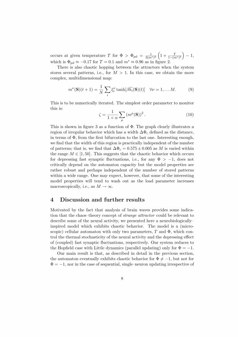
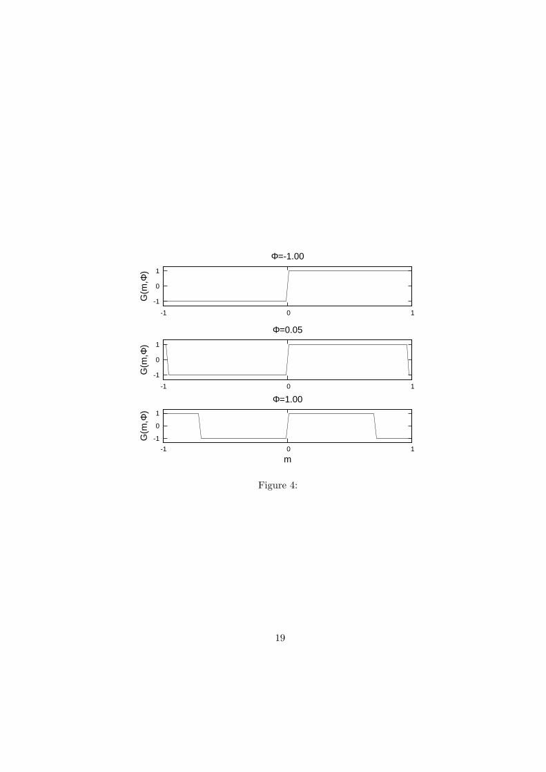
This is not the first time in which chaos is reported to occur duringthe retrieval process in attractor neural networks; see, for instance, (Wanget al., 1990; Bolle and Vink, 1996; Dominguez and Theumann, 1997; Poonand Barahona, 2001; Caroppo et al., 1999; Mainieri and Jr., 2002; Katayamaet al., 2003). One may say, however, that we provide in this paper a moregeneral and microscopic setting than before and, in fact, the onset of chaoshere could not be phenomenologically predicted. That is, the same mi-croscopic mechanism, namely (1) and (3), does not imply chaotic behaviorif updating is by a sequential single–variable process (Cortes et al., 2006).Another possible comparison is by noticing that, in any case, whether oneproceeds more or less phenomenologically, the result is a map mt+1 = G(mt).We obtained the gain function G after coarse graining of (4)–(7), and theMonte Carlo simulations fitting the map behavior just involve neurons sub-ject to the local fields (2), so that we are only left in the two cases with thenoise parameter Φ to be tuned. In contrast, some related works, in order todeepen more directly on the possible origin of chaos, use the gain functionitself as a parameter. It is also remarkable that, e.g., in (Dominguez andTheumann, 1997) and some related work (Caroppo et al., 1999; Mainieri andJr., 2002; Katayama et al., 2003), the gain function is phenomenologicallycontrolled by tuning the neuron threshold for firing, θi. The threshold func-tion thus becomes a relevant parameter, and it ensues that any meaningfulchaos in this context requires non–zero threshold. This is because, in thesecases, the local fields and, consequently, the overlaps, are lineal, which forcesone to induce chaos by other means. Interesting enough, our gain function in(8) has either a sigmoid shape or an oscillating one, as illustrated for T = 0in figure 4. Only the latter case allows for hopping between the attractorsand, eventually, for chaotic behavior.

Finally, we demonstrate an interesting property of our automaton dur-ing retrieval. This is the fact that, in the chaotic regime, the system isextremely susceptible to external influences. A rather stringent test of thisis its behavior concerning mixture or spin–glass steady states, which are un-suited in relation with associative memory. Even though these states mayoccur at low T, this system —unlike other cases— easily escapes from them

9

under a very small external stimulus. This is illustrated in figure 5 whichalso demonstrates a general feature, namely, some strong correlation be-tween chaos and a vivid response to the environment. This nicely conformsexpectations, as mentioned above, that chaotic itinerancy might be a rathergeneral strategy of nature.

5 Acknowledgments

We acknowledge with thanks very useful discussions with David R.C. Domınguez,Pedro L. Garrido, Sabine Hilfiker and Hilbert J. Kappen, and financial sup-port from MEyC and FEDER, project No. FIS2005-00791, Junta de An-dalucıa project FQM-165 and EPSRC–funded COLAMN project EP/CO1084/1.

10

References

Amit, D. J. (1989). Modeling brain function: the world of attractor neuralnetwork. Cambridge University Press.

Ashwin, P. and Timme, M. (2005). Nonlinear dynamics: When instabilitymakes sense. Nature, 436:36–37.

Barrie, J. M., Freeman, W. J., and Lenhart, M. (1996). Modulation bydiscriminative training of spatial patterns of gamma EEG amplitude andphase in neocortex of rabbits. J. Neurophysiol., 76:520–539.

Bibitchkov, D., Herrmann, J. M., and Geisel, T. (2002). Pattern storageand processing in attractor networks with short-time synaptic dynamics.Network: Comput. Neural Syst., 13:115–129.

Bolle, D. and Vink, B. (1996). On the dynamics of analogue neurons withnonsigmoidal gain functions. Physica A, 223:293–308.

Caroppo, D., Mannarelli, M., Nardulli, G., and Stramaglia, S. (1999). Chaosin neural networks with a nonmonotonic transfer function. Phys. Rev. E,60:2186–2192.

Coolen, A. C. C. (2001). Statistical mechanics of recurrent neural networks:II. Dynamics. In Moss, F. and Gielen, C., editors, HandBook of BiologicalPhysics, volume 4, pages 619–684. Elsevier Science.

Cortes, J. M., Garrido, P. L., Marro, J., and Torres, J. J. (2004). Switchingbetween memories in neural automata with synaptic noise. Neurocomput-ing, 58-60:67–71.

Cortes, J. M., Torres, J. J., Marro, J., Garrido, P. L., and Kappen, H. J.(2006). Effects of fast presynaptic noise in attractor neural networks.Neural Comp., 13:614–633.

Dominguez, R. R. C. and Theumann, W. (1997). Generalization and chaosin a layered neural network. J. Phys. A: Math. Gen., 30:1403–1414.

Faure, P. and Korn, H. (2001). Is there chaos in the brain? i. concepts ofnonlinear dynamics and methods of investigation. C. R. Acad. Sci. III,324:773–793.

Franks, K. M., Stevens, C. F., and Sejnowski, T. J. (2003). Independentsources of quantal variability at single glutamatergic synapses. J. Neu-rosci., 23:3186–3195.

11

Freeman, W. J. (2003). Evidence from human scalp electroencephalogramsof global chaotic itinerancy. Chaos, 13:1067–1077.

Ganguly, N., Das, A., Maji, P., Sikdar, B. K., and Chaudhuri, P. P. (2003).Evolving cellular automata based associative memory for pattern recog-nition. In Monien, B., Prasanna, V., and Vajapeyam, S., editors, HighPerformance Computing - HiPC 2001 : 8th International Conference,volume 2228, pages 115–124. Springer-Verlag.

Hansel, D. and Sompolinsky, H. (1996). Chaos and synchrony in a model ofa hypercolumn in visual cortex. J. Comput. Neurosci., 3:7–34.

Kaneko, K. and Tsuda, I. (2001). Complex Systems: Chaos and Beyond. AConstructive Approach with Applications in Life Sciences. Springer.

Katayama, K., Sakata, Y., and Horiguchi, T. (2003). Layered neural net-works with non-monotonic transfer functions. Physica A, 317:270–298.

Kiel, L. D. and Elliot, E., editors (1996). Chaos Theory in the Social Sci-ences: Foundations and Applications. The University of Michigan Press.

Korn, H. and Faure, P. (2003). Is there chaos in the brain? ii. experimentalevidence and related models. C. R. Biol., 326:787–840.

Lu, Q., Shen, G., and Yu, R. (2003). A chaotic approach to maintain thepopulation diversity of genetic algorithm in network training. Comput.Biol. Chem., 27:363–371.

Mainieri, M. and Jr., R. E. (2002). Retrieval and chaos in extremely dilutednon-monotonic neural networks. Physica A, 311:581–589.

Marro, J. and Dickman, R. (1999). Nonequilibrium Phase Transitions inLattice Models. Cambridge University Press.

Pantic, L., Torres, J. J., Kappen, H. J., and Gielen, S. C. A. M. (2002).Associative memory with dynamic synapses. Neural Comp., 14:2903–2923.

Poon, C. S. and Barahona, M. (2001). Titration of chaos with added noise.Proc. Natl. Acad. Sci. USA, 98:7107–7112.

Rabinovich, M. I. and Abarbanel, H. D. I. (1998). The role of chaos in neuralsystems. Neuroscience, 87:5–14.

12

Schweighofer, N., Doya, K., Fukai, H., Chiron, J. V., Furukawa, T., andKawato, M. (2004). Chaos may enhance information transmission in theinferior olive. Proc. Natl. Acad. Sci. USA, 101:4655–4660.

Strogatz, S. (2003). Sync: The Emerging Science of Spontaneous Order.Hyperion, N.Y.

Tsodyks, M. V., Pawelzik, K., and Markram, H. (1998). Neural networkswith dynamic synapses. Neural Comp., 10:821–835.

Tsuda, I. (2001). Toward an interpretation of dynamic neural activity interms of chaotic dynamical systems. Behav. Brain Sci., 24:793–810.

Wang, L., Pichler, E. E., and Ross, J. (1990). Oscillations and chaos inneural networks: An exactly solvable model. Proc. Natl. Acad. Sci. USA,87:9467–9471.

Zador, A. (1998). Impact of synaptic unreliability on the information trans-mitted by spiking neurons. J. Neurophysiol., 79:1219–1229.

13

Figure Captions

Figure 1: Monte Carlo time–evolution of the overlap between the automa-ton current state and the given stored pattern for M = 1, N = 104 neurons,T = 0.1, and different values of Φ, as indicated. This illustrates, from topto bottom, the fixed point solution in the absence of any synaptic noise, i.e.,Φ = −1, a cyclic behavior, the onset of irregular periodic behavior, and fullyirregular and regular jumping between the two attractors corresponding, re-spectively, to the given pattern, m ≡ m1 = 1, and its anti–pattern m = −1—the only possibilities in this case with M = 1.

Figure 2: Bifurcation diagram and associated Lyapunov exponent demon-strating chaotic activity for some (but not all) values of the depressing co-efficient Φ. The upper graph shows, for M = 1, the steady overlap betweenthe current state and the given pattern as a function of Φ. This is fromMonte Carlo simulations of a network with N = 104 neurons. The bottomgraph depicts the corresponding Lyapunov exponent, λ, as obtained fromthe map (8). This confirms the existence of chaotic windows, in which λ > 0.The temperature parameter is set T = 0.1 in both cases; this is low enoughso that the effect of thermal fluctuations is negligible compared to that ofsynaptic noise.

Figure 3: The function ζ (Φ) , as defined in the main text, obtained fromMonte Carlo simulations at T = 0.15 for N = 104 neurons and M = 20stored patterns generated at random. A region of irregular behavior whichextends for ∆Φc, as indicated, is depicted. The insets show the time evo-lution of 4 out of the 20 overlaps within the irregular region, namely, forΦ = 0.11.

Figure 4: The gain function in (8) versus mt for T = 0 and differentvalues of Φ, as indicated. It is to be remarked that this function is non-sigmoidal, namely, oscillatory, which allows for hopping between the attrac-tors for Φ > 0, while it is monotonic in the Hopfield case Φ = −1.

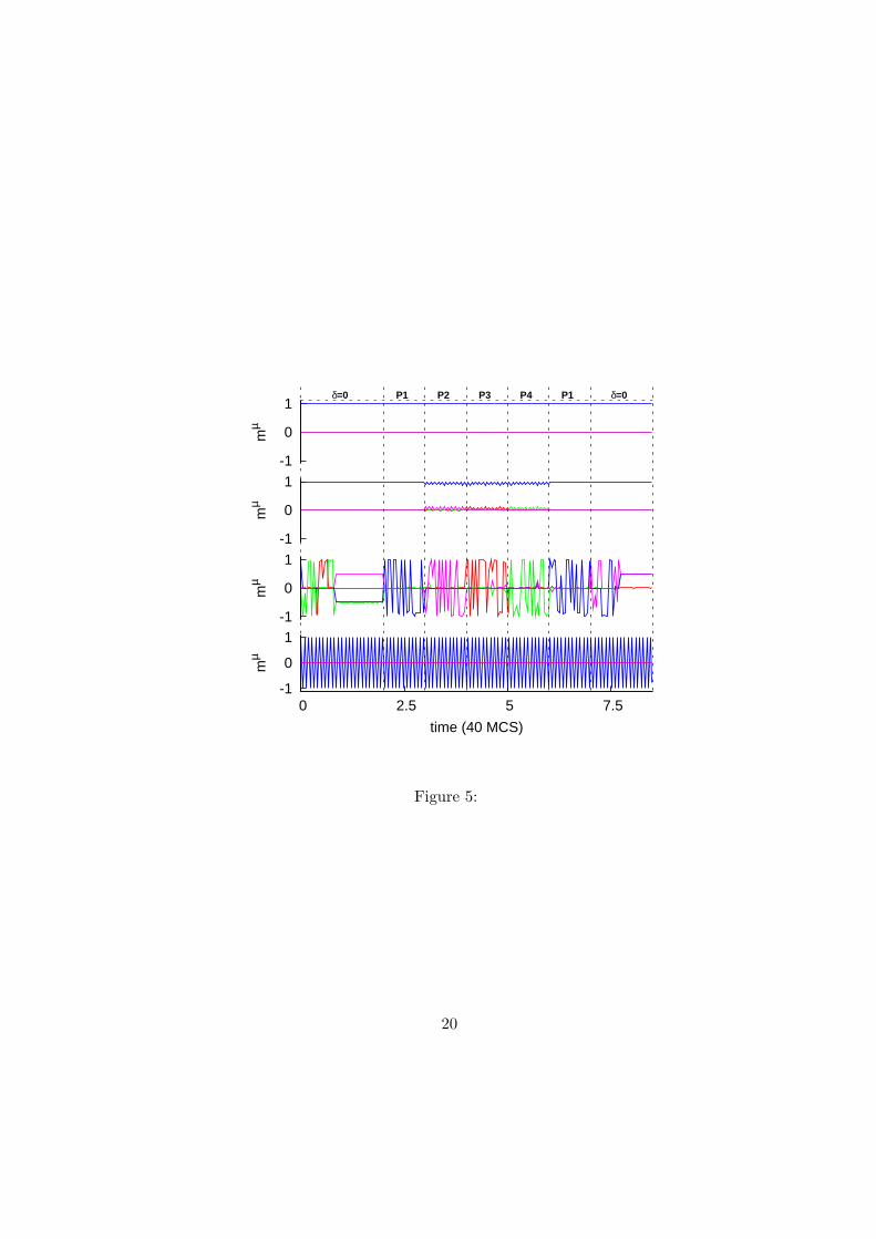
Figure 5: Time evolution of the overlap mµ in a Monte Carlo simula-tion with N =104 neurons, M = 4 stored (random) patterns, T = 0.05,and, from top to bottom, Φ = −0.2, −0.1, 0.12, and 0.2. This illustratesthat, under regular behavior (as for the first two top graphs and the bottomone), the system is unable to respond to a week external stimulus. This issimulated as an extra local field, hext

i = δξµi , where δ = 0.05 and µ changes

14

(µ = 1, 2, 3, 4, 1) every 40 MCS as indicated by Pµ above the top graph.The situation is qualitatively different when the regime is chaotic, as forΦ = 0.12 in this figure. After some wandering in the evolution that weshow here, the system activity is trapped in a mixture state around t = 80MCS. However, the external stimulus induces jumping to the more corre-lated attractor, and so on. That is, chaos importantly enhances the networksensitivity. To obtain a similar behavior during the regular regimes, onewould need to increase considerably the external force δ.

15

-1

0

1

500 525 550 575 600

m

Φ=-1.00

-1

0

1

500 525 550 575 600

m

Φ=-0.10

-1

0

1

500 525 550 575 600

m

Φ=-0.02

-1

0

1

500 525 550 575 600

m

Φ=0.03

-1

0

1

500 525 550 575 600

m

time (MCS)

Φ=0.05

Figure 1:

16

-1

-0.5

0

0.5

1

-1 -0.5 0 0.5 1

m

-20

-16

-12

-8

-4

0

4

-1 -0.5 0 0.5 1

λ

Φ

Figure 2:

17

1

0.5

0

-1 -0.5 0 0.5

ζ

Φ

∆Φc

Φ=0.11

-1 0 1

0 1 2 3 4 5

m1

time (102 MCS)

-1 0 1

m6

-1 0 1

m11

-1 0 1

m20

Figure 3:

18

-1

0

1

-1 0 1

G(m

,Φ)

Φ=-1.00

-1

0

1

-1 0 1

G(m

,Φ)

Φ=0.05

-1

0

1

-1 0 1

G(m

,Φ)

m

Φ=1.00

Figure 4:

19

1

0

-1 0 2.5 5 7.5

mµ

time (40 MCS)

1

0

-1

mµ

1

0

-1

mµ

1

0

-1

mµ

δ=0 P1 P2 P3 P4 P1 δ=0

Figure 5:

20