Machine Learning Strategies for Time Series Predictiondi.ulb.ac.be/map/gbonte/ftp/time_ser.pdf · Discovery of the molecular pathways regulating pancreatic beta cell dysfunction and

Machine Learning Strategies for TimeSeries Prediction

Machine Learning Summer School(Hammamet, 2013)

Gianluca Bontempi

Machine Learning Group, Computer Science Department

Boulevard de Triomphe - CP 212

http://www.ulb.ac.be/di

Machine Learning Strategies for Prediction – p. 1/128

Introducing myself• 1992: Computer science engineer (Politecnico di Milano, Italy),

• 1994: Researcher in robotics in IRST, Trento, Italy,

• 1995: Researcher in IRIDIA, ULB Artificial Intelligence Lab, Brussels,

• 1996-97: Researcher in IDSIA, Artificial Intelligence Lab, Lugano,Switzerland,

• 1998-2000: Marie Curie fellowship in IRIDIA, ULB Artificial IntelligenceLab, Brussels,

• 2000-2001: Scientist in Philips Research, Eindhoven, The Netherlands,

• 2001-2002: Scientist in IMEC, Microelectronics Institute, Leuven,Belgium,

• since 2002: professor in Machine Learning, Modeling and Simulation,Bioinformatics in ULB Computer Science Dept., Brussels,

• since 2004: head of the ULB Machine Learning Group (MLG).

• since 2013: director of the Interuniversity Institute of Bioinformatics inBrussels (IB)2, ibsquare.be.


... and in terms of distances

According to MathSciNet

•• Distance from Erdos= 5

• Distance from Zaiane= 6

• Distance from Deisenroth= 8


ULB Machine Learning Group (MLG)• 3 professors, 10 PhD students, 5 postdocs.

• Research topics: Knowledge discovery from data, Classification, Computationalstatistics, Data mining, Regression, Time series prediction, Sensor networks,

Bioinformatics, Network inference.

• Computing facilities: high-performing cluster for analysis of massive datasets,Wireless Sensor Lab.

• Website: mlg.ulb.ac.be.

• Scientific collaborations in ULB: Hopital Jules Bordet, Laboratoire de Médecine

experimentale, Laboratoire d’Anatomie, Biomécanique et Organogénèse (LABO),Service d’Anesthesie (ERASME).

• Scientific collaborations outside ULB: Harvard Dana Farber (US), UCL MachineLearning Group (B), Politecnico di Milano (I), Universitá del Sannio (I), Inst Rech

Cliniques Montreal (CAN).


ULB-MLG: recent projects1. Machine Learning for Question Answering (2013-2014).

2. Adaptive real-time machine learning for credit card fraud detection (2012-2013).

3. Epigenomic and Transcriptomic Analysis of Breast Cancer (2012-2015).

4. Discovery of the molecular pathways regulating pancreatic beta cell dysfunction

and apoptosis in diabetes using functional genomics and bioinformatics: ARC(2010-2015)

5. ICT4REHAB - Advanced ICT Platform for Rehabilitation (2011-2013)

6. Integrating experimental and theoretical approaches to decipher the molecular

networks of nitrogen utilisation in yeast: ARC (2006-2010).

7. TANIA - Système d’aide à la conduite de l’anesthésie. WALEO II project fundedby the Région Wallonne (2006-2010)

8. "COMP2SYS" (COMPutational intelligence methods for COMPlex SYStems)MARIE CURIE Early Stage Research Training funded by the EU (2004-2008).


What you are supposed to know

• Basic notions of probability and statistics

• Random variable

• Expectation, variance, covariance

• Least-squares

What you are expected to get acquainted with

• Foundations of statistical machine learning

• How to build a predictive model from data

• Strategies for forecasting

What will remain

• Interest, curiosity for machine learning

• taste for prediction

• Contacts

• Companion webpagehttp://www.ulb.ac.be/di/map/gbonte/mlss.html


Outline• Notions of time series (30 mins )

• conditional probability

• Machine learning for prediction (45 mins )• bias/variance• parametric and structural identification• validation• model selection

• feature selection

• COFFEE BREAK

• Local learning (15 mins )

• Forecasting: one-step and multi-step-ahed (30 mins )

• Some applications (15 mins )• time series competitions• wireless sensor

• biomedical

• Future directions and perspectives (15 mins )


What is machine learning?Machine learning is that domain of computational intelligence which isconcerned with the question of how to construct computer programs thatautomatically improve with experience. [16]

Reductionist attitude: ML is just a buzzword which equates to statistics plusmarketing

Positive attitude: ML paved the way to the treatment of real problems relatedto data analysis, sometimes overlooked by statisticians (nonlinearity,classification, pattern recognition, missing variables, adaptivity,optimization, massive datasets, data management, causality,representation of knowledge, parallelisation)

Interdisciplinary attitude: ML should have its roots on statistics andcomplements it by focusing on: algorithmic issues, computationalefficiency, data engineering.


Why study machine learning?

• Machine learning is cool.

• Practical way to understand: All models are wrong but some are useful...

• The fastest way to become a data scientist ... the sexiest job in the 21stcentury

• Someone who knows statistics better than a computer scientists andprograms better than a statistician...


Notion of time series


Time seriesDefinition A time series is a sequence of observations st ∈ R, usuallyordered in time.

Examples of time series in every scientific and applied domain:

• Meteorology: weather variables, like temperature, pressure, wind.

• Economy and finance: economic factors (GNP), financial indexes,exchange rate, spread.

• Marketing: activity of business, sales.

• Industry: electric load, power consumption, voltage, sensors.

• Biomedicine: physiological signals (EEG), heart-rate, patienttemperature.

• Web: clicks, logs.

• Genomics: time series of gene expression during cell cycle.


Why studying time series?

There are various reasons:

Prediction of the future based on the past.

Control of the process producing the series.

Understanding of the mechanism generating the series.

Description of the salient features of the series.


Univariate discrete time series

• Quantities, like temperature and voltage, change in a continuous way.

• In practice, however, the digital recording is made discretely in time.

• We shall confine ourselves to discrete time series (which however takecontinuous values).

• Moreover we will consider univariate time series, where one type ofmeasurement is made repeatedly on the same object or individual.

• Multivariate time series are out of the scope of this presentation butrepresent an important topic in the domain.


A general modelLet an observed discrete univariate time series be s1, . . . , sT . This meansthat we have T numbers which are observations on some variable made at T

equally distant time points, which for convenience we label 1, 2, . . . , T .

A fairly general model for the time series can be written

st = g(t) + ϕt t = 1, . . . , T

The observed series is made of two components

Systematic part: g(t), also called signal or trend, which is a determisticfunction of time

Stochastic sequence: a residual term ϕt, also called noise, which follows aprobability law.


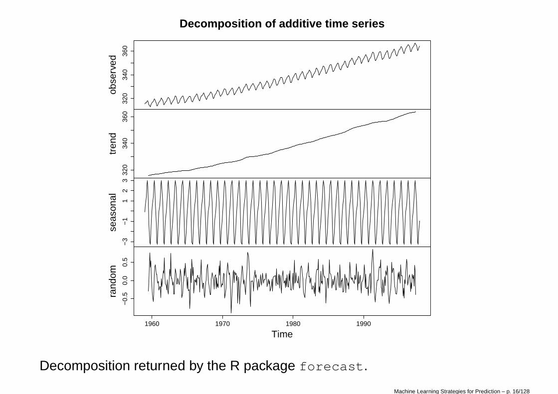
Types of variationTraditional methods of time-series analysis are mainly concerned withdecomposing the variation of a series st into:

Trend : this is a long-term change in the mean level, eg. an increasing trend.

Seasonal effect : many time series (sale figures, temperature readings) exhibitvariation which is seasonal (e.g. annual) in period. The measure and theremoval of such variation brings to deseasonalized data.

Irregular fluctuations : after trend and cyclic variations have been removedfrom a set of data, we are left with a series of residuals, which may ormay not be completely random.

We will assume here that once we have detrended and deseasonalized theseries, we can still extract information about the dependency between thepast and the future. Henceforth ϕt will denote the detrended anddeseasonalized series.


320

340

360

obse

rved

320

340

360

tren

d−

3−

11

23

seas

onal

−0.

50.

00.

5

1960 1970 1980 1990

rand

om

Time

Decomposition of additive time series

Decomposition returned by the R package forecast.


Probability and dependency• Forecasting a time series is possible since future depends on the past or

analogously because there is a relationship between the future and thepast. However this relation is not deterministic and can hardly be writtenin an analytical form.

• An effective way to describe a nondeterministic relation between twovariables is provided by the probability formalism.

• Consider two continuous random variables ϕ1 and ϕ2 representing forinstance the temperature today (time t1) and tomorrow (t2). We tend tobelieve that ϕ1 could be used as a predictor of ϕ2 with some degree ofuncertainty.

• The stochastic dependency between ϕ1 and ϕ2 is resumed by the jointdensity p(ϕ1, ϕ2) or equivalently by the conditional probability

p(ϕ2|ϕ1) =p(ϕ1, ϕ2)

p(ϕ1)

• If p(ϕ2|ϕ1) 6= p(ϕ2) then ϕ1 and ϕ2 are not independent or equivalentlythe knowledge of the value of ϕ1 reduces the uncertainty about ϕ2.


Stochastic processes• The stochastic approach to time series makes the assumption that a

time series is a realization of a stochastic process (like tossing anunbiased coin is the realization of a discrete random variable with equalhead/tail probability).

• A discrete-time stochastic process is a collection of random variables ϕt,t = 1, . . . , T defined by a joint density

p(ϕ1, . . . , ϕT )

• Statistical time-series analysis is concerned with evaluating theproperties of the probability model which generated the observed timeseries.

• Statistical time-series modeling is concerned with inferring the propertiesof the probability model which generated the observed time series from a

limited set of observations .


Strictly stationary processes• Predicting a time series is possible if and only if the dependence

between values existing in the past is preserved also in the future.

• In other terms, though measures change, the stochastic rule underlyingtheir realization does not. This aspect is formalized by the notion ofstationarity.

• Definition A stochastic process is said to be strictly stationary if the jointdistribution of ϕt1

, ϕt2, . . . , ϕtn

is the same as the joint distribution ofϕt1+k, ϕt2+k, . . . , ϕtn+k for all n, t1, . . . , tn and k.

• In other words shifting the time origin by an amount k has no effect onthe joint distribution which depends only on the intervals betweent1, . . . , tn.

• This implies that the (marginal) distribution of ϕt is the same for all t.

• The definition holds for any value of n.

• Let us see what does it mean in practice for n = 1 and n = 2.


Propertiesn=1 : If ϕt is strictly stationary and its first two moments are finite, we have

E[ϕt] = µt = µ, Var [ϕt] = σ2t = σ2

n=2 : Furthermore the autocovariance function γ(t1, t2) depends only on thelag k = t2 − t1 and may be written by

γ(k) = Cov[ϕt, ϕt+k] = E[

(ϕt − µ)(ϕt+k − µ)]

• In order to avoid scaling effects, it is useful to introduce theautocorrelation function

ρ(k) =γ(k)

σ2=

γ(k)

γ(0)

• Another relevant function is the the partial autocorrelation function π(k)

where π(k), k > 1 measures the degree of association between ϕt andϕt−k when the effects of the intermediary lags 1, . . . , k − 1 are removed


Weak stationarity• A less restricted definition of stationarity concerns only the first two

moments of ϕt

Definition A process is called second-order stationary or weakly stationary

if its mean is constant and its autocovariance function depends only onthe lag.

• No assumptions are made about higher moments than those of secondorder.

• Strict stationarity implies weak stationarity but not viceversa in general.

Definition A process is called normal is the joint distribution ofϕt1

, ϕt2, . . . , ϕtn

is multivariate normal for all t1, . . . , tn.

• In the special case of normal processes, weak stationarity implies strictstationarity. This is due to the fact that a normal process is completelyspecified by the mean and the autocovariance function.


Estimators of first momentsHere you will find some common estimators of the two first moments of atime series:

• The empirical mean is given by

µ =

∑T

t=1 ϕt

T

• The empirical autocovariance function is given by

γ(k) =

∑T−k

t=1 (ϕt − µ)(ϕt+k − µ)

T − k − 1, k < T − 2

• The empirical autocorrelation function is given by

ρ(k) =γ(k)

γ(0)


Some examples of stochastic

processes


Purely random processes• It consists of a sequence of random variables ϕt which are mutually

independent and identically distributed. For each t and k

p(ϕt+k|ϕt) = p(ϕt+k)

• It follows that this process has constant mean and variance. Also

γ(k) = Cov[ϕt, ϕt+k] = 0

for k = ±1,±2, . . . .

• A purely random process is strictly stationary.

• A purely random process is sometimes called white noise by engineers.

• An example of purely random process is the series of numbers drawn bya roulette wheel in a casino.


Example: Gaussian purely random

0 200 400 600 800 1000

−3

−2

−1

01

23

White noise

t

y


Example: autocorrelation function

0 5 10 15 20 25 30

0.0

0.2

0.4

0.6

0.8

1.0

Lag

AC

F

Series y


Random walk• Suppose that wt is a discrete, purely random process with mean µ and

variance σ2w

.

• A process ϕt is said to be a random walk if

ϕt = ϕt−1 + wt

• The next value of a random walk is obtained by summing a randomshock to the latest value.

• If ϕ0 = 0 then

ϕt =t

∑

i=1

wi

• E[ϕt] = tµ and Var [ϕt] = tσ2w

.

• As the mean and variance change with t the process is non-stationary.


Random walk (II)• The first differences of a random walk given by

∇ϕt = ϕt − ϕt−1

form a purely random process, which is stationary.

• Examples of time series which behave like random walks are• stock prices on successive days.• the path traced by a molecule as it travels in a liquid or a gas,• the search path of a foraging animal


Ten random walksLet w ∼ N (0, 1).

0 50 100 150 200 250 300 350 400 450 500−40

−30

−20

−10

0

10

20

30

40

50

60Random walks


Autoregressive processes• Suppose that wt is a purely random process with mean zero and

variance σ2w

.

• A process ϕt is said to be an autoregressive process of order n (also anAR(n) process) if

ϕt = α1ϕt−1 + · · · + αnϕt−n + wt

• This means that the next value is a linear weighted sum of the past n

values plus a random shock.

• Finite memory filter.

• If w is a normal variable, ϕt will be normal too.

• Note that this is like a linear regression model where ϕ is regressed noton independent variables but on its past values (hence the prefix “auto”).

• The properties of stationarity depends on the values αi, i = 1, . . . , n.


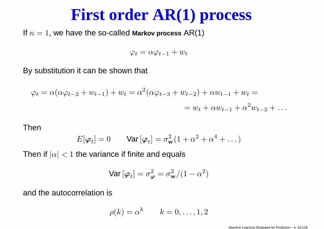
First order AR(1) processIf n = 1, we have the so-called Markov process AR(1)

ϕt = αϕt−1 + wt

By substitution it can be shown that

ϕt = α(αϕt−2 + wt−1) + wt = α2(αϕt−3 + wt−2) + αwt−1 + wt =

= wt + αwt−1 + α2wt−2 + . . .

ThenE[ϕt] = 0 Var [ϕt] = σ2

w(1 + α2 + α4 + . . . )

Then if |α| < 1 the variance if finite and equals

Var [ϕt] = σ2ϕ

= σ2w

/(1 − α2)

and the autocorrelation is

ρ(k) = αk k = 0, . . . , 1, 2


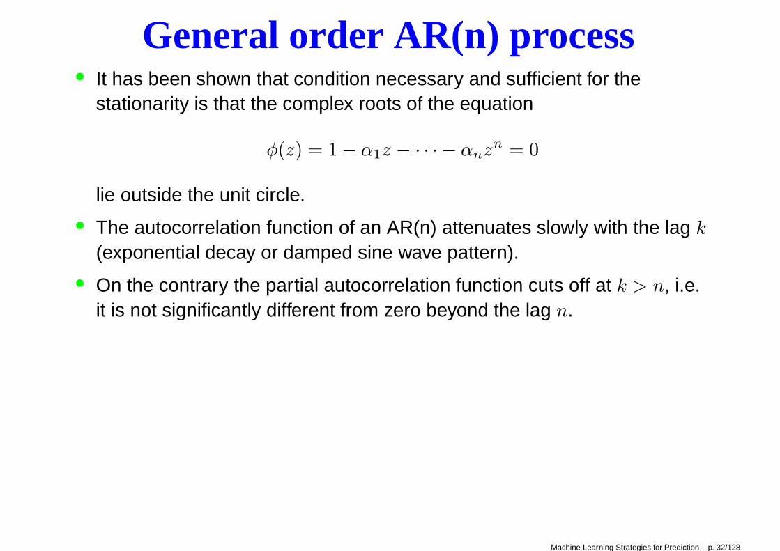
General order AR(n) process• It has been shown that condition necessary and sufficient for the

stationarity is that the complex roots of the equation

φ(z) = 1 − α1z − · · · − αnzn = 0

lie outside the unit circle.

• The autocorrelation function of an AR(n) attenuates slowly with the lag k

(exponential decay or damped sine wave pattern).

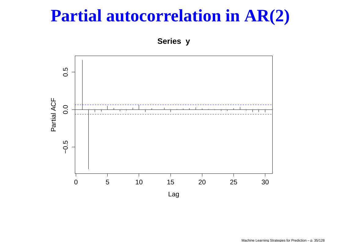
• On the contrary the partial autocorrelation function cuts off at k > n, i.e.it is not significantly different from zero beyond the lag n.


Example: AR(2)

0 200 400 600 800 1000

05

1015

AR(2)

t

y


Example: AR(2)

0 5 10 15 20 25 30

−0.

50.

00.

51.

0

Lag

AC

F

Series y


Partial autocorrelation in AR(2)

0 5 10 15 20 25 30

−0.

50.

00.

5

Lag

Par

tial A

CF

Series y


Fitting an autoregressive process

The estimation of an autoregressive process to a set of dataDT = {ϕ1, . . . , ϕT } demands the resolution of two problems:

1. The estimation of the order n of the process. This is typically supportedby the analysis of the partial autocorrelation function.

2. The estimation of the set of parameters {α1, . . . , αn}.


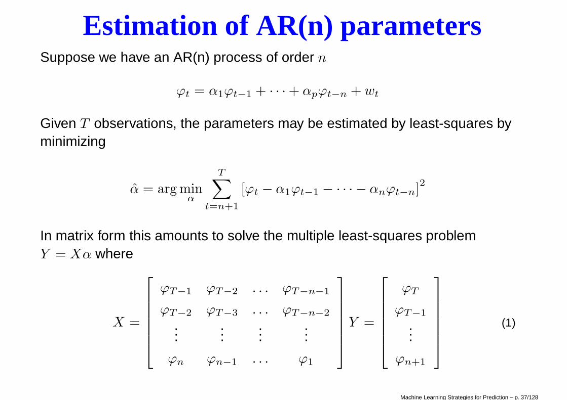
Estimation of AR(n) parametersSuppose we have an AR(n) process of order n

ϕt = α1ϕt−1 + · · · + αpϕt−n + wt

Given T observations, the parameters may be estimated by least-squares byminimizing

α = arg minα

T∑

t=n+1

[ϕt − α1ϕt−1 − · · · − αnϕt−n]2

In matrix form this amounts to solve the multiple least-squares problemY = Xα where

X =

ϕT−1 ϕT−2 . . . ϕT−n−1

ϕT−2 ϕT−3 . . . ϕT−n−2

......

......

ϕn ϕn−1 . . . ϕ1

Y =

ϕT

ϕT−1

...

ϕn+1

(1)


Least-squares estimation of AR(n) parms• Let N be the number of rows of X . In order to estimate the AR(n)

parameters we compute the least-squares estimator

α = arg mina

N∑

i=1

(yi − xTi a)2 = arg min

a

(

(Y − Xa)T (Y − Xa))

• It can be shown thatα = (XT X)−1XT Y

where the XT X matrix is a symmetric [n × n] matrix which plays animportant role in multiple linear regression.

• Conventional linear regression theory provides also confidence intervaland significativity tests for the AR(n) coefficients.

• A recursive version of least-squares, i.e. where time samples arrivesequentially, is provided by the RLS algorithm.


From linear to nonlinear setting


The NAR representation• AR models assume that the relation between past and future is linear

• Once we assume that the linear assumption does not hold, we mayextend the AR formulation to a Nonlinear Auto Regressive (NAR)formulation

ϕt = f (ϕt−1, ϕt−2, . . . , ϕt−n) + w(t)

where the missing information is lumped into a noise term w.

• In what follows we will consider this relationship as a particular instanceof a dependence

y = f(x) + w

between a multidimensional input x ∈ X ⊂ Rn and a scalar output y ∈ R.

• NOTA BENE. In what follows y will denote the next value ϕt to bepredicted and

x = [ϕt−1, ϕt−2, . . . , ϕt−n]

will denote the n-dimensional input vector also known as embeddingvector.


Nonlinear vs. linear time series

The advantage of linear models are numerous:

• the least-squares α estimate can be expressed in an analytical form

• the least-squares α estimate can be easily calculated through matrixcomputation.

• statistical properties of the estimator can be easily defined.

• recursive formulation for sequential updating are avaialble.

• the relation between empirical and generalization error is known,

BUT...


Nonlinear vs. linear time series

• linear methods interpret all the structure in a time series through linearcorrelation

• deterministic linear dynamics can only lead to simple exponential orperiodically oscillating behavior, so all irregular behavior is attributed toexternal noise while deterministic nonlinear equations could producevery irregular data,

• in real problems it is extremely unlikely that the variables are linked by alinear relation.

In practice, the form of the relation is often unknown and only a limitedamount of samples is available.


Machine learning for prediction


Supervised learning

TRAINING DATASET

UNKNOWN

DEPENDENCY

INPUT OUTPUTERROR

PREDICTION

MODELPREDICTION

From now on we consider the prediction problem as a problem of supervised

learning problem, where we have to infer from historical data the possiblynonlinear dependance between the input (past embedding vector) and theoutput (future value).

Statistical machine learning is the discipline concerned with this problem.


The regression plus noise form• A typical way of representing the unknown input/output relation is the

regression plus noise form

y = f(x) + w

where f(·) is a deterministic function and the term w represents thenoise or random error. It is typically assumed that w is independent of x

and E[w] = 0.

• Suppose that we have available a training set {〈xi, yi〉 : i = 1, . . . , N},where xi = (xi1, . . . , xin) and yi, generated according to the previousmodel.

• The goal of a learning procedure is to estimate a model f(x) which isable to give a good approximation of the unknown function f(x).

• But how to choose f , if we do not know the probability distributionunderlying the data and we have only a limited training set?


A simple example withn = 1

−2 −1 0 1 2

−5

05

1015

x

Y

NOTA BENE: this is NOT a time series ! y = ϕt, x = ϕt−1. The horizontal axisdoes not represent time but the past value of the series.


Model degree 1

−2 −1 0 1 2

−5

05

1015

x

Y

Training error= 2 degree= 1

f(x) = α0 + α1x


Model degree 3

−2 −1 0 1 2

−5

05

1015

x

Y

Training error= 0.92 degree= 3

f(x) = α0 + α1x + · · · + α3x3


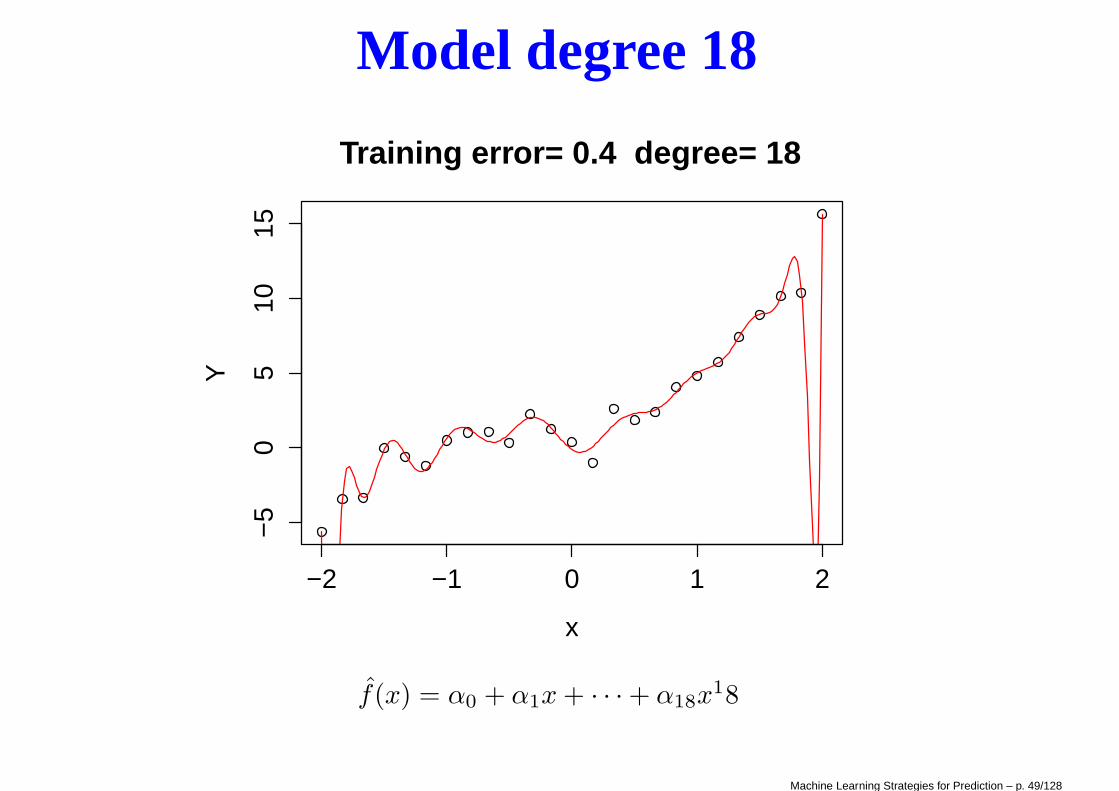
Model degree 18

−2 −1 0 1 2

−5

05

1015

x

Y

Training error= 0.4 degree= 18

f(x) = α0 + α1x + · · · + α18x18


Generalization and overfitting• How to estimate the quality of a model? Is the training error a good

measure of the quality?

• The goal of learning is to find a model which is able to generalize , i.e.able to return good predictions for input values independent of thetraining set.

• In a nonlinear setting, it is possible to find models with such a complicatestructure that they have null training errors. Are these models good?

• Typically NOT. Since doing very well on the training set could meandoing badly on new data.

• This is the phenomenon of overfitting .

• Using the same data for training a model and assessing it is typically awrong procedure, since this returns an over optimistic assessment of themodel generalization capability.


Bias and variance of a model• A fundamental result of estimation theory shows that the

mean-squared-error, i.e. a measure of the generalization quality of anestimator can be decomposed into three terms:

MISE = σ2w

+ squared bias + variance

where the intrinsic noise term reflects the target alone, the bias reflectsthe target’s relation with the learning algorithm and the variance termreflects the learning algorithm alone.

• This result is purely theoretical since these quantities cannot bemeasured on the basis of a finite amount of data.

• However, this result provides insight about what makes accurate alearning process.


The bias/variance trade-off• The first term is the variance of y around its true mean f(x) and cannot

be avoided no matter how well we estimate f(x), unless σ2w

= 0.

• The bias measures the difference in x between the average of theoutputs of the hypothesis functions f over the set of possible DN andthe regression function value f(x)

• The variance reflects the variability of the guessed f(x, αN ) as onevaries over training sets of fixed dimension N . This quantity measureshow sensitive the algorithm is to changes in the data set, regardless tothe target.


The bias/variance dilemma• The designer of a learning machine has not access to the term MISE but

can only estimate it on the basis of the training set. Hence, thebias/variance decomposition is relevant in practical learning since itprovides a useful hint about the features to control in order to make theerror MISE small.

• The bias term measures the lack of representational power of the classof hypotheses. To reduce the bias term we should consider complexhypotheses which can approximate a large number of input/outputmappings.

• The variance term warns us against an excessive complexity of theapproximator. This means that a class of too powerful hypotheses runsthe risk of being excessively sensitive to the noise affecting the trainingset; therefore, our class could contain the target but it could bepractically impossible to find it out on the basis of the available dataset.


• In other terms, it is commonly said that an hypothesis with large bias butlow variance underfits the data while an hypothesis with low bias butlarge variance overfits the data.

• In both cases, the hypothesis gives a poor representation of the targetand a reasonable trade-off needs to be found.

• The task of the model designer is to search for the optimal trade-offbetween the variance and the bias term, on the basis of the availabletraining set.


Bias/variance trade-off

complexity

generalizationerror

Bias

Variance

Underfitting Overfitting


The learning procedureA learning procedure aims at two main goals:

1. to choose a parametric family of hypothesis f(x, α) which contains orgives good approximation of the unknown function f (structural

identification ).

2. within the family f(x, α), to estimate on the basis of the training set DN

the parameter αN which best approximates f (parametric identification ).

In order to accomplish that, a learning procedure is made of two nestedloops:

1. an external structural identification loop which goes through differentmodel structures

2. an inner parametric identification loop which searches for the bestparameter vector within the family structure.


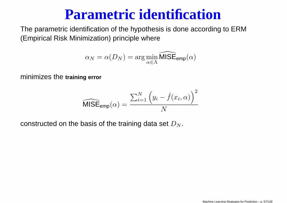
Parametric identificationThe parametric identification of the hypothesis is done according to ERM(Empirical Risk Minimization) principle where

αN = α(DN ) = arg minα∈Λ

MISEemp(α)

minimizes the training error

MISEemp(α) =

∑N

i=1

(

yi − f(xi, α))2

N

constructed on the basis of the training data set DN .


Parametric identification (II)• The computation of αN requires a procedure of multivariate optimization

in the space of parameters.

• The complexity of the optimization depends on the form of f(·).

• In some cases the parametric identification problem may be an NP-hardproblem.

• Thus, we must resort to some form of heuristic search.

• Examples of parametric identification procedure are linear least-squaresfor linear models and backpropagated gradient-descent for feedforwardneural networks.


Model assessment• We have seen before that the training error is not a good estimator (i.e. it

is too optimistic) of the generalization capability of the learned model.

• Two alternative exists:

1. Complexity-based penalty criteria

2. Data-driven validation techniques


Complexity-based penalization• In conventional statistics, various criteria have been developed, often in

the context of linear models, for assessing the generalizationperformance of the learned hypothesis without the use of furthervalidation data.

• Such criteria take the form of a sum of two terms

GPE = MISEemp + complexity term

where the complexity term represents a penalty which grows as thenumber of free parameters in the model grows.

• This expression quantifies the qualitative consideration that simplemodels return high training error with a reduced complexity term whilecomplex models have a low training error thanks to the high number ofparameters.

• The minimum for the criterion represents a trade-off betweenperformance on the training set and complexity.


Complexity-based penalty criteriaIf the input/output relation is linear, well-known examples of complexity basedcriteria are:

• the Final Prediction Error (FPE)

FPE = MISEemp(αN )1 + p/N

1 − p/N

with p = n + 1,

• the Generalized Cross-Validation (GCV)

GCV = MISEemp(αN )1

(1 − pN

)2

• the Akaike Information Criterion (AIC)

AIC =p

N−

1

NL(αN )

where L(·) is the log-likelihood function,


• the Cp criterion proposed by Mallows

Cp =MISEemp(αN )

σ2w

+ 2p − N

where σ2w is an estimate of the variance of noise,

• the Predicted Squared Error (PSE)

PSE = MISEemp(αN ) + 2σ2w

p

N

where σ2w is an estimate of the variance of noise.


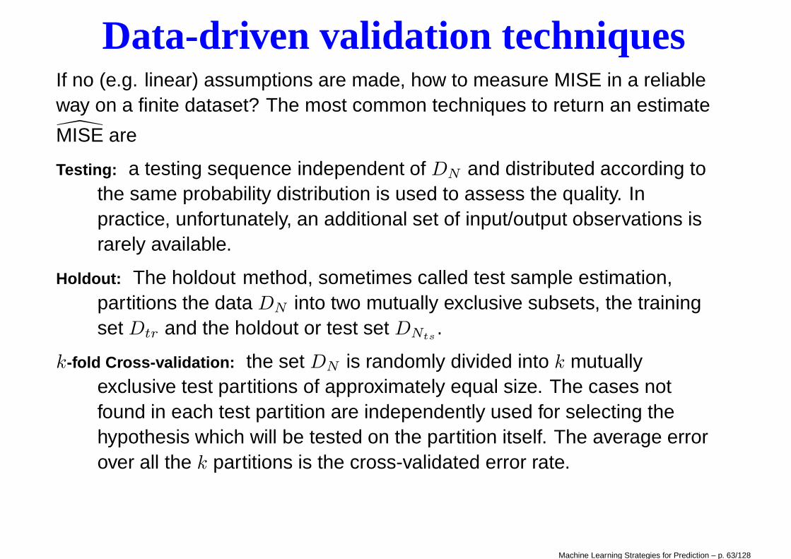
Data-driven validation techniquesIf no (e.g. linear) assumptions are made, how to measure MISE in a reliableway on a finite dataset? The most common techniques to return an estimate

MISE are

Testing: a testing sequence independent of DN and distributed according tothe same probability distribution is used to assess the quality. Inpractice, unfortunately, an additional set of input/output observations israrely available.

Holdout: The holdout method, sometimes called test sample estimation,partitions the data DN into two mutually exclusive subsets, the trainingset Dtr and the holdout or test set DNts

.

k-fold Cross-validation: the set DN is randomly divided into k mutuallyexclusive test partitions of approximately equal size. The cases notfound in each test partition are independently used for selecting thehypothesis which will be tested on the partition itself. The average errorover all the k partitions is the cross-validated error rate.


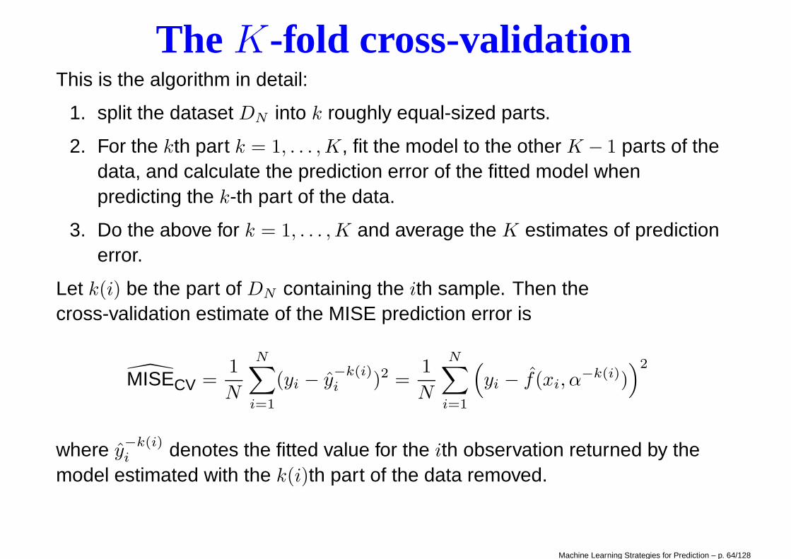
The K-fold cross-validationThis is the algorithm in detail:

1. split the dataset DN into k roughly equal-sized parts.

2. For the kth part k = 1, . . . , K, fit the model to the other K − 1 parts of thedata, and calculate the prediction error of the fitted model whenpredicting the k-th part of the data.

3. Do the above for k = 1, . . . , K and average the K estimates of predictionerror.

Let k(i) be the part of DN containing the ith sample. Then thecross-validation estimate of the MISE prediction error is

MISECV =1

N

N∑

i=1

(yi − y−k(i)i )2 =

1

N

N∑

i=1

(

yi − f(xi, α−k(i))

)2

where y−k(i)i denotes the fitted value for the ith observation returned by the

model estimated with the k(i)th part of the data removed.


10-fold cross-validationK = 10: at each iteration 90% of data are used for training and the remaining10% for the test.

90%

10%


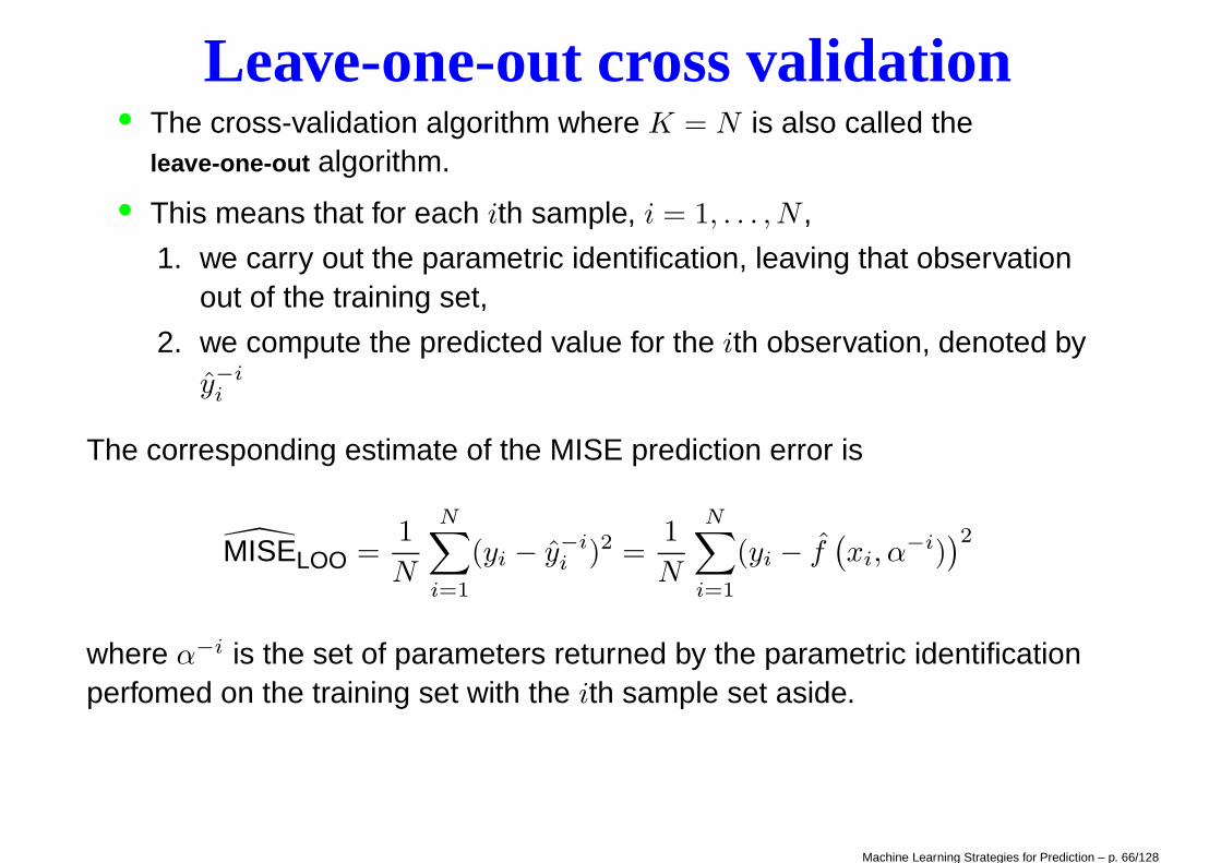
Leave-one-out cross validation• The cross-validation algorithm where K = N is also called the

leave-one-out algorithm.

• This means that for each ith sample, i = 1, . . . , N ,

1. we carry out the parametric identification, leaving that observationout of the training set,

2. we compute the predicted value for the ith observation, denoted byy−i

i

The corresponding estimate of the MISE prediction error is

MISELOO =1

N

N∑

i=1

(yi − y−ii )2 =

1

N

N∑

i=1

(yi − f(

xi, α−i)

)2

where α−i is the set of parameters returned by the parametric identificationperfomed on the training set with the ith sample set aside.


Model selection• Model selection concerns the final choice of the model structure

• By structure we mean:• family of the approximator (e.g. linear, non linear) and if nonlinear

which kind of learner (e.g. neural networks, support vectormachines, nearest-neighbours, regression trees)

• the value of hyper parameters (e.g. number of hidden layers, numberof hidden nodes in NN, number of neighbors in KNN, number oflevels in trees)

• number and set of input variables

• this choice is typically the result of a compromise between differentfactors, like the quantitative measures, the personal experience of thedesigner and the effort required to implement a particular model inpractice.

• Here we will consider only quantitative criteria. Two are the possibleapproaches:

1. the winner-takes-all approach

2. the combination of estimators approach.Machine Learning Strategies for Prediction – p. 67/128

Model selection

N

REALIZATION

STOCHASTIC PROCESS

VALIDATION

CLASSES of HYPOTHESIS

LEARNED MODEL

TRAINING SET

MODEL SELECTION

PARAMETRIC IDENTIFICATION

IDENTIFICATION

,,

, ,

,

,

STRUCTURAL

α?

ΛSΛ2Λ1

GN

1α1

N

α1

N

α2

N

α2

N

αN

s

αN

s

GN

2 GN

S

GN

2GN

1 GN

S


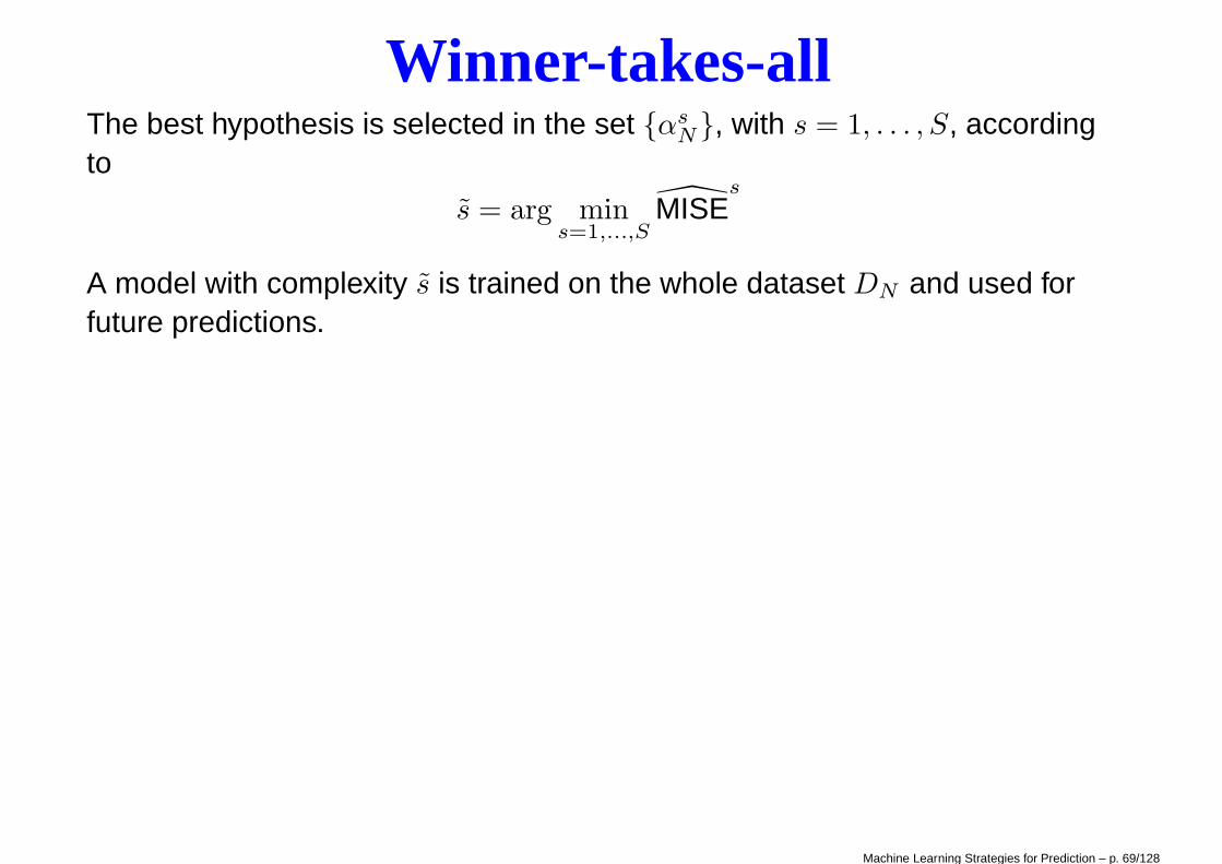
Winner-takes-allThe best hypothesis is selected in the set {αs

N}, with s = 1, . . . , S, accordingto

s = arg mins=1,...,S

MISEs

A model with complexity s is trained on the whole dataset DN and used forfuture predictions.


Winner-takes-all pseudo-code1. for s = 1, . . . , S: (Structural loop)

• for j = 1, . . . , N

(a) Inner parametric identification (for l-o-o):

αsN−1 = arg min

α∈Λs

∑

i=1:N,i 6=j

(yi − f(xi, α))2

(b) ej = yj − f(xj , αsN−1)

• MISELOO(s) = 1N

∑N

j=1 e2j

2. Model selection: s = arg mins=1,...,S MISELOO(s)

3. Final parametric identification:αs

N = arg minα∈Λs

∑N

i=1(yi − f(xi, α))2

4. The output prediction model is f(·, αsN )


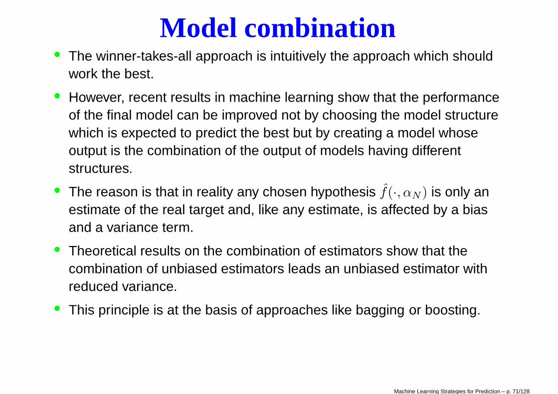
Model combination• The winner-takes-all approach is intuitively the approach which should

work the best.

• However, recent results in machine learning show that the performanceof the final model can be improved not by choosing the model structurewhich is expected to predict the best but by creating a model whoseoutput is the combination of the output of models having differentstructures.

• The reason is that in reality any chosen hypothesis f(·, αN ) is only anestimate of the real target and, like any estimate, is affected by a biasand a variance term.

• Theoretical results on the combination of estimators show that thecombination of unbiased estimators leads an unbiased estimator withreduced variance.

• This principle is at the basis of approaches like bagging or boosting.


Feature selection problem• Machine learning algorithms are known to degrade in performance

(prediction accuracy) when faced with many inputs (aka features) thatare not necessary for predicting the desired output.

• In the feature selection problem, a learning algorithm is faced with theproblem of selecting some subset of features upon which to focus itsattention, while ignoring the rest.

• Using all available features may negatively affect generalizationperformance, especially in the presence of irrelevant or redundantfeatures.

• Feature selection can be seen as an instance of model selectionproblem.


Benefits and drawbacks of feature selectionThere are many potential benefits of feature selection:

• facilitating data visualization and data understanding,

• reducing the measurement and storage requirements,

• reducing training and utilization times of the final model,

• defying the curse of dimensionality to improve prediction performance.

Drawbacks are

• the search for a subset of relevant features introduces an additional layerof complexity in the modelling task. The search in the model hypothesisspace is augmented by another dimension: the one of finding theoptimal subset of relevant features.

• additional time for learning.


Curse of dimensionality• The error of the best model decreases with n but the mean integrated

squared error of models increases faster than linearly in n.

• In high dimensions, all data sets are sparse.

• In high dimensions, the number of possible models to considerincreases superexponenetially in n.

• In high dimensions, all datasets show multicollinearity.

• As n increases the amount of local data goes to zero.

• For a uniform distribution around a query point xq the amount of datathat are contained in a ball of radius r < 1 centered in xq grows like rn.


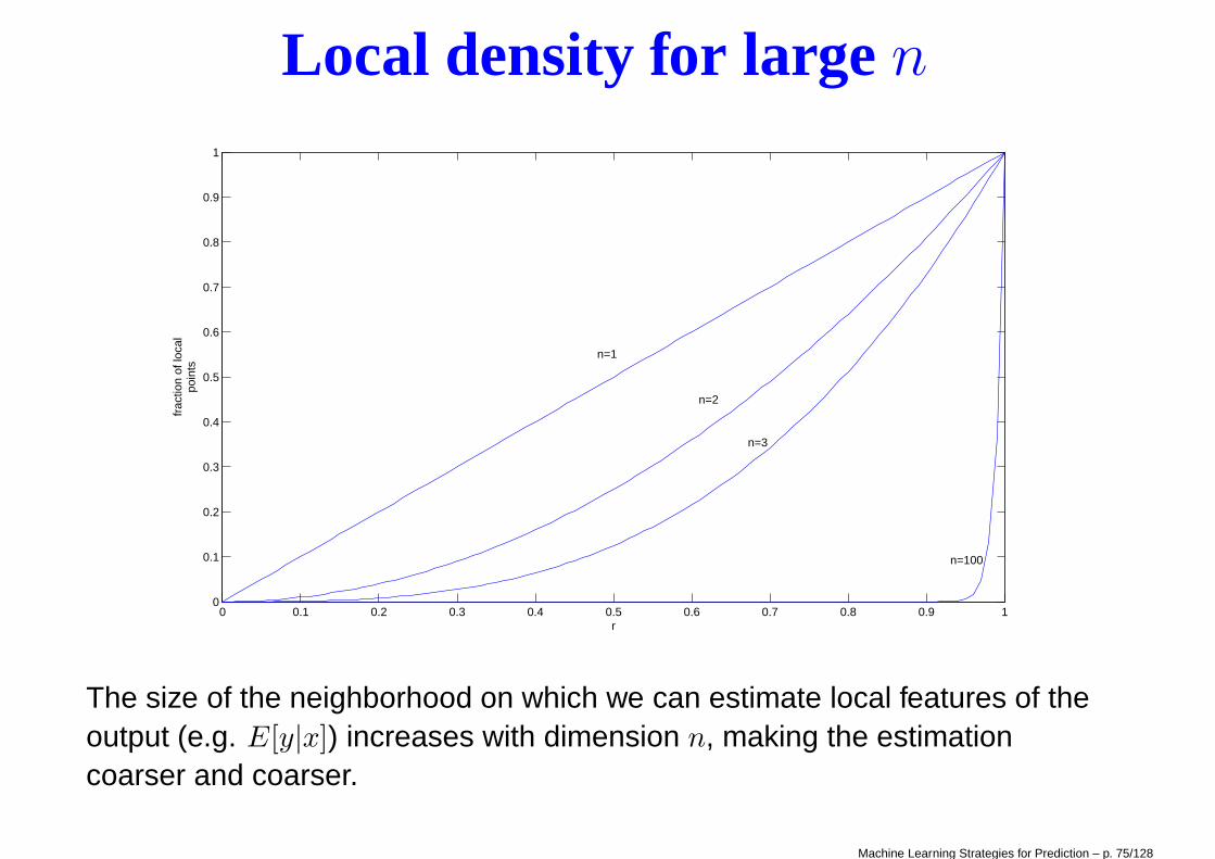
Local density for large n

0 0.1 0.2 0.3 0.4 0.5 0.6 0.7 0.8 0.9 10

0.1

0.2

0.3

0.4

0.5

0.6

0.7

0.8

0.9

1

r

frac

tion

of lo

cal

poin

ts

n=1

n=2

n=3

n=100

The size of the neighborhood on which we can estimate local features of theoutput (e.g. E[y|x]) increases with dimension n, making the estimationcoarser and coarser.


Methods of feature selectionTwo are the main approaches to feature selection:

Filter methods: they are preprocessing methods. They attempt to assess themerits of features from the data, ignoring the effects of the selectedfeature subset on the performance of the learning algorithm. Examplesare methods that select variables by ranking them through compressiontechniques (like PCA or clustering) or by computing correlation with theoutput.

Wrapper methods: these methods assess subsets of variables according totheir usefulness to a given predictor. The method conducts a search fora good subset using the learning algorithm itself as part of the evaluationfunction. The problem boils down to a problem of stochastic state spacesearch. Example are the stepwise methods proposed in linearregression analysis.

Embedded methods: they perform variable selection as part of the learningprocedure and are usually specific to given learning machines.Examples are classification trees, random forests, and methods basedon regularization techniques (e.g. lasso)


Local learning


Local modeling procedureThe learning of a local model in xq ∈ Rn can be summarized in these steps:

1. Compute the distance between the query xq and the training samplesaccording to a predefined metric.

2. Rank the neighbors on the basis of their distance to the query.

3. Select a subset of the k nearest neighbors according to the bandwidthwhich measures the size of the neighborhood.

4. Fit a local model (e.g. constant, linear,...).

Each of the local approaches has one or more structural (or smoothing)parameters that control the amount of smoothing performed.Let us focus on the bandwidth selection.


The bandwidth trade-off: overfit

e

q

��

��

��

��

��

��

��

��

��

��

��

��

��

��

��

��

��

��

��

��

��

��

��

x

y

��

��

��

��

��

��

��

��

��

��

��

��

��

��

��

��

��

��

��

��

��

��

��

��

��

��

x

y

Too narrow bandwidth ⇒ overfitting ⇒ large prediction error e.In terms of bias/variance trade-off, this is typically a situation of high variance.


The bandwidth trade-off: underfit

e

q

��

��

��

��

��

��

��

��

��

��

��

��

��

��

��

��

��

��

��

��

��

��

x

y

��

��

��

��

��

��

��

��

��

��

��

��

��

��

��

��

��

��

��

��

��

��

��

��

��

��

��

��

��

��

��

��

��

��

��

��

x

y

Too large bandwidth ⇒ underfitting ⇒ large prediction error e

In terms of bias/variance trade-off, this is typically a situation of high bias.


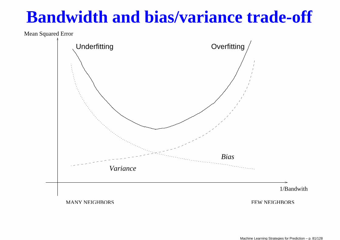
Bandwidth and bias/variance trade-offMean Squared Error

1/Bandwith

FEW NEIGHBORSMANY NEIGHBORS

Bias

Variance

Underfitting Overfitting


The PRESS statistic• Cross-validation can provide a reliable estimate of the algorithm

generalization error but it requires the training process to be repeated K

times, which sometimes means a large computational effort.

• In the case of linear models there exists a powerful statistical procedureto compute the leave-one-out cross-validation measure at a reducedcomputational cost

• It is the PRESS (Prediction Sum of Squares) statistic, a simple formulawhich returns the leave-one-out (l-o-o) as a by-product of theleast-squares.


Leave-one-out for linear models

PARAMETRIC IDENTIFICATION ON N-1 SAMPLES

PUT THE j-th SAMPLE ASIDE

TEST ON THE j-th SAMPLE

PARAMETRIC IDENTIFICATION

ON N SAMPLESN TIMES

TRAINING SET

PRESS STATISTIC

LEAVE-ONE-OUT

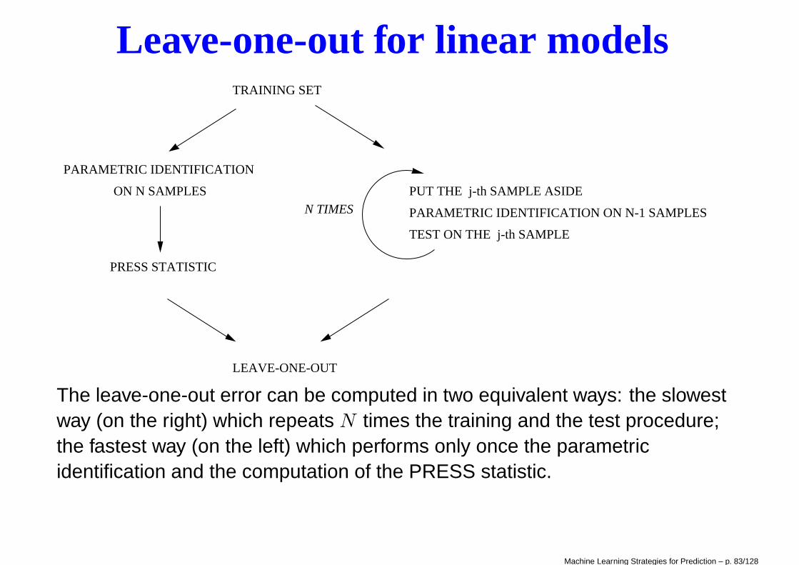
The leave-one-out error can be computed in two equivalent ways: the slowestway (on the right) which repeats N times the training and the test procedure;the fastest way (on the left) which performs only once the parametricidentification and the computation of the PRESS statistic.


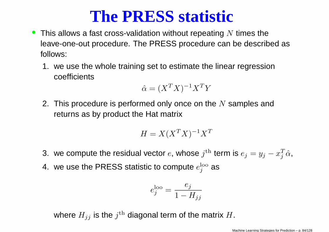
The PRESS statistic• This allows a fast cross-validation without repeating N times the

leave-one-out procedure. The PRESS procedure can be described asfollows:

1. we use the whole training set to estimate the linear regressioncoefficients

α = (XT X)−1XT Y

2. This procedure is performed only once on the N samples andreturns as by product the Hat matrix

H = X(XT X)−1XT

3. we compute the residual vector e, whose jth term is ej = yj − xTj α,

4. we use the PRESS statistic to compute elooj as

elooj =

ej

1 − Hjj

where Hjj is the jth diagonal term of the matrix H.


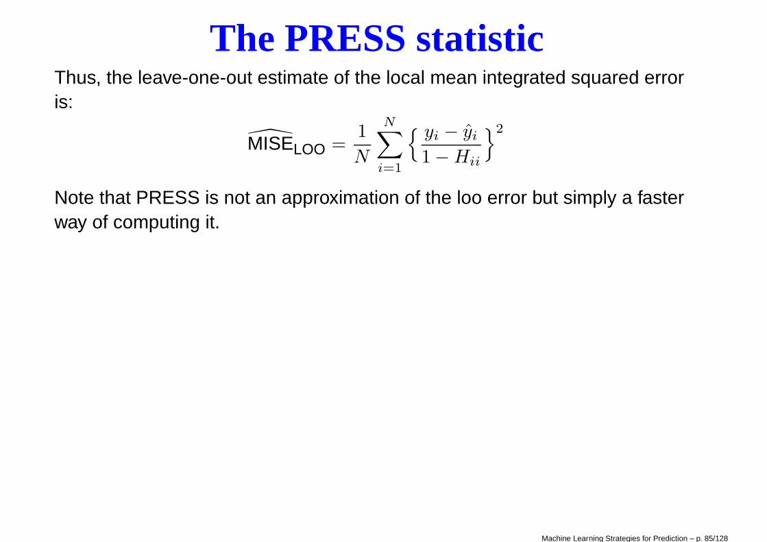
The PRESS statisticThus, the leave-one-out estimate of the local mean integrated squared erroris:

MISELOO =1

N

N∑

i=1

{ yi − yi

1 − Hii

}2

Note that PRESS is not an approximation of the loo error but simply a fasterway of computing it.


Selection of the number of neighbours• For a given query point xq, we can compute a set of predictions

yq(k) = xTq α(k)

, together with a set of associated leave-one-out error vectors

MISELOO(k) for a number of neighbors ranging in [kmin, kmax].

• If the selection paradigm, frequently called winner-takes-all, is adopted,the most natural way to extract a final prediction yq, consists incomparing the prediction obtained for each value of k on the basis of theclassical mean square error criterion:

yq = xTq α(k), with k = arg min

kMISELOO(k)


Local Model combination• As an alternative to the winner-takes-all paradigm, we can use a

combination of estimates.

• The final prediction of the value yq is obtained as a weighted average ofthe best b models, where b is a parameter of the algorithm.

• Suppose the predictions yq(k) and the loo errors MISELOO(k) have beenordered creating a sequence of integers {ki} so that

MISELOO(ki) ≤ MISELOO(kj), ∀i < j. The prediction of yq is given by

yq =

∑b

i=1 ζiyq(ki)∑b

i=1 ζi

,

where the weights are the inverse of the mean square errors:

ζi = 1/MISELOO(ki).


Forecasting


One step-ahead and iterated prediction• Once a model of the embedding mapping is available, it can be used for

two objectives: one-step-ahead prediction and iterated prediction.

• In one-step-ahead prediction, the n previous values of the series areavailable and the forecasting problem can be cast in the form of ageneric regression problem

• In literature a number of supervised learning approaches have beenused with success to perform one-step-ahead forecasting on the basisof historical data.


One step-ahead prediction

f

ϕt-2

z -1

z -1

z -1

ϕt-3

ϕt-n

ϕt-1

z -1

ϕt

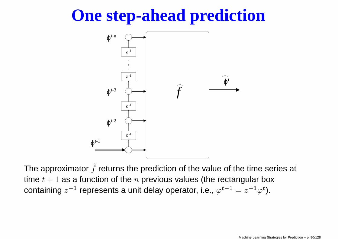
The approximator f returns the prediction of the value of the time series attime t + 1 as a function of the n previous values (the rectangular boxcontaining z−1 represents a unit delay operator, i.e., ϕt−1 = z−1ϕt).


Nearest-neighbor one-step-ahead forecastst

−−

y

t−11t−16 t−1t−6t

We want to predict at time t − 1 the next value of the series y of order n = 6.The pattern yt−16, yt−15, . . . , yt−11 is the most similar to the pattern{yt−6, yt−5, . . . , yt−1}. Then, the prediction yt = yt−10 is returned.


Multi-step ahead prediction• The prediction of the value of a time series H > 1 steps ahead is called

H-step-ahead prediction.

• We classify the methods for H-step-ahead prediction according to twofeatures: the horizon of the training criterion and the single-output ormulti-output nature of the predictor.


Multi-step ahead prediction strategiesThe most common strategies are

1. Iterated: the model predicts H steps ahead by iterating aone-step-ahead predictor whose parameters are optimized to minimizethe training error on one-step-ahead forecast (one-step-ahead trainingcriterion).

2. Iterated strategy where parameters are optimized to minimize thetraining error on the iterated htr-step-ahead forecast (htr-step-aheadtraining criterion) where 1 < htr ≤ H.

3. Direct: the model makes a direct forecast at time t + h − 1, h = 1, . . . , H

by modeling the time series in a multi-input single-output form

4. Direc: direct forecast but the input vector is extended at each step withpredicted values.

5. MIMO: the model returns a vectorial forecast by modeling the timeseries in a multi-input multi-output form


Iterated (or recursive) prediction• In the case of iterated prediction, the predicted output is fed back as

input for the next prediction.

• Here, the inputs consist of predicted values as opposed to actualobservations of the original time series.

• As the feedback values are typically distorted by the errors made by thepredictor in previous steps, the iterative procedure may produceundesired effects of accumulation of the error.

• Low performance is expected in long horizon tasks. This is due to thefact that they are essentially models tuned with a one-step-aheadcriterion which is not capable of taking temporal behavior into account.


Iterated prediction

f

ϕt-2

z -1

z -1

z -1

z -1

ϕt-3

ϕt-n

ϕt-1

z -1

ϕt

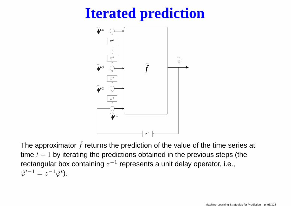
The approximator f returns the prediction of the value of the time series attime t + 1 by iterating the predictions obtained in the previous steps (therectangular box containing z−1 represents a unit delay operator, i.e.,ϕt−1 = z−1ϕt).


Iterated with h-step training criterion• This strategy adopts one-step-ahead predictors but adapts the model

selection criterion in order to take into account the multi-step-aheadobjective.

• Methods like Recurrent Neural Networks belong to such class. Theirrecurrent architecture and the associated training algorithm (temporalbackpropagation) are suitable to handle the time-dependent nature ofthe data.

• In [4] we proposed an adaptation of the Lazy Learning algorithm wherethe number of neighbors is optimized in order to minimize theleave-one-out error over an horizon larger than one. This techniqueranked second in the 1998 KULeuven Time Series competition.

• A similar technique has been proposed by [14] who won the competition.


Conventional and iterated leave-one-out

a)

3

12

4

5

3

e (3)cv

12

3

45

e (3)

b)

it

12

4

5

3

12 3

45

3


Santa Fe time series A

0 200 400 600 800 1000

050

100

150

200

250

Santa Fe time series A

t

y

The A chaotic time series has a training set of 1000 values: the task is topredict the continuation for 100 steps, starting from different points.


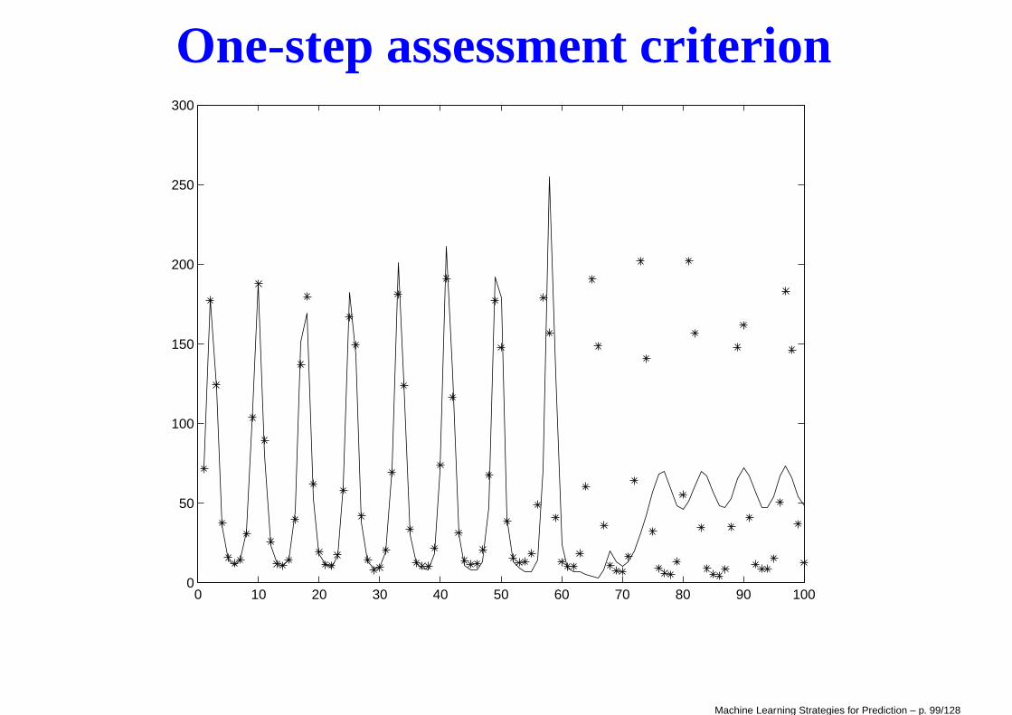
One-step assessment criterion

0 10 20 30 40 50 60 70 80 90 1000

50

100

150

200

250

300


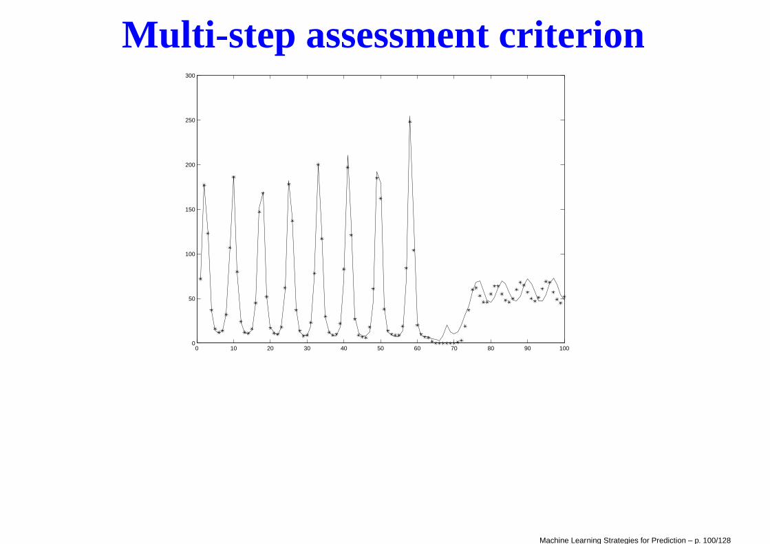
Multi-step assessment criterion

0 10 20 30 40 50 60 70 80 90 1000

50

100

150

200

250

300


Direct strategy• The Direct strategy [22, 17, 7] learns independently H models fh

ϕt+h−1 = fh(ϕt−1, . . . , ϕt−n) + wt+h−1

with h ∈ {1, . . . , H} and returns a multi-step forecast by concatenatingthe H predictions.

• Several machine learning models have been used to implement theDirect strategy for multi-step forecasting tasks, for instance neuralnetworks [10], nearest neighbors [17] and decision trees [21].

• Since the Direct strategy does not use any approximated values tocompute the forecasts, it is not prone to any accumulation of errors,since each model is tailored for the horizon it is supposed to predict.

• Notwithstanding, it has some weaknesses.


Direct strategy limitations• Since the H models are learned independently no statistical

dependencies between the predictions ϕt+h−1, h = 1, . . . , H [3, 5, 10] isguaranteed.

• Direct methods often require higher functional complexity [20] thaniterated ones in order to model the stochastic dependency between twoseries values at two distant instants [9].

• This strategy demands a large computational time since the number ofmodels to learn is equal to the size of the horizon.


DirRec strategy• The DirRec strategy [18] combines the architectures and the principles

underlying the Direct and the Recursive strategies.

• DirRec computes the forecasts with different models for everyhorizon (like the Direct strategy) and, at each time step, it enlarges theset of inputs by adding variables corresponding to the forecasts of theprevious step (like the Recursive strategy).

• Unlike the previous strategies, the embedding size n is not the same forall the horizons. In other terms, the DirRec strategy learns H models fh

from the time series where

ϕt+h−1 = fh(ϕt+h−1, . . . , ϕt−n) + wt+h−1

with h ∈ {1, . . . , H}.

• The technique is prone to the curse of dimensionality. The use of featureselection is recommended for large h.


MIMO strategy• This strategy [3, 5] (also known as Joint strategy [10]) avoids the

simplistic assumption of conditional independence between futurevalues made by the Direct strategy [3, 5] by learning a singlemultiple-output model

[ϕt+H−1, . . . , ϕt] = F (ϕt−1, . . . , ϕt−n) + w

where F : Rd → RH is a vector-valued function [15], and w ∈ RH is anoise vector with a covariance that is not necessarily diagonal [13].

• The forecasts are returned in one step by a multiple-inputmultiple-output regression model.

• In [5] we proposed a multi-output extension of the local learningalgorithm.

• Other multi-output regression model could be taken into considerationlike multi-output neural networks or partial least squares.


Time series dependencies

t+3

ϕ ϕ

ϕ ϕ

ϕ

t−1 t

t+1 t+2

n = 2 NAR dependency ϕt = f(ϕt−1, ϕt−2) + w(t).


Iterated modeling of dependencies

t+3

ϕ ϕ

ϕ

t+1ϕ ϕ t+2

tt−1


Direct modeling of dependencies

t+3

ϕ ϕ

ϕ ϕ

ϕ

t−1 t

t+1 t+2


MIMO strategy• The rationale of the MIMO strategy is to model, between the predicted

values, the stochastic dependency characterizing the time series. Thisstrategy avoids the conditional independence assumption made by theDirect strategy as well as the accumulation of errors which plagues theRecursive strategy.

• So far, this strategy has been successfully applied to several real-worldmulti-step time series forecasting tasks [3, 5, 19, 2].

• However, the wish to preserve the stochastic dependencies constrainsall the horizons to be forecasted with the same model structure. Sincethis constraint could reduce the flexibility of the forecastingapproach [19], a variant of the MIMO strategy (called DIRMO) has beenproposed in [19, 2] .

• Extensive validation on the 111 times series of the NN5 competitionshowed that MIMO are invariably better than single-output approaches.


Validation of time series methods• The huge variety of strategies and algorithms that can be used to infer a

predictor from observed data asks for a rigorous procedure ofcomparison and assessment.

• Assessment demands benchmarks and benchmarking procedure.

• Benchmarks can be defined by using• Simulated data obtained by simulating AR, NAR and other stochastic

processes. This is particular useful for validating theoreticalproperties in terms of bias/variance.

• Public domain benchmarks, like the one provided by Time SeriesCompetitions.

• Real measured data


Competitions• Santa Fe Time Series Prediction and Analysis Competition (1994) [22]:

• International Workshop on Advanced Black-box techniques for nonlinearmodeling Competition (Leuven, Belgium; 1998)

• NN3 competition [8]: 111 monthly time series drawn from homogeneouspopulation of empirical business time series.

• NN5 competition [1]: 111 time series of the daily retirement amountsfrom independent cash machines at different, randomly selectedlocations across England.

• Kaggle competition.


Accuracy measuresLet

et+h = ϕt+h − ϕt+h

represent the error of the forecast ϕt+h at the horizon h = 1, . . . , H. Aconventional measure of accuracy is the Normalized Mean Squared Error

NMSE =

∑H

h=1(ϕt+h − ϕt+h)2∑H

h=1(ϕt+h − µ)2

This quantity is smaller than one if the predictor performs better than thenaivest predictor, i.e. the average µ.Other measures rely on relative or percentage error

pet+h = 100ϕt+h − ϕt+h

ϕt+h

like

MAPE =

∑H

h=1 |pet+h|

H


Applications in my lab


MLG projects on forecasting• Low-energy streaming of wireless sensor data

• Decision support in anesthesia

• Side-channel attack


Low-energy streaming of wireless sensor data• In monitoring applications, only an approximation to sensor readings is

sufficient (e.g. ±0.5C, ±2% humidity, ..). In this context a Dual PredictionScheme is effective.

• A sensor node is provided with a time series prediction modelϕt = f(ϕt−1, α) (e.g. autoregressive models) and a learning method foridentifying the best set of parameters α (e.g. recursive least squares).

• The sensor node then sends the parameters of the model instead of theactual data to the recipient. The recipient node then runs the models toreconstruct an approximation of the data stream collected on the distantnode.

• The sensor node also runs the prediction model. When its predictionsdiverges by more than ±ǫ from the actual reading, a new model is sentto the recipient.

• This allows to reduce the communication effort if an appropriate model isrun by the sensor node.

• Since the cost of transmission is much larger than the cost ofcomputation, in realistic situations this scheme allows economy of powerconsumption. Machine Learning Strategies for Prediction – p. 114/128

Low-energy streaming of wireless sensor data

0 5 10 15 20

20

25

30

35

40

45

Accuracy: 2°C

Constant model

Time (Hour)

Temperature (°C)

! !! !!! !! ! ! !! ! ! ! ! ! ! ! ! !


Adaptive model selectionTradeoff: more complex models predict better measurements but have ahigher number of parameters

Model complexity

Metric

Communication costs

Model error

AR(p) : si[t] =

p∑

j=1

θjsi[t − j]


Adaptive Model SelectionWe proposed an Adaptive Model Selection strategy [11] that

• takes into account the cost of sending model parameters,

• allows sensor nodes to determine autonomously the model which bestfits their measurements,

• provides a statistically sound selection mechanism to discard poorlyperforming models,

• gave in experimental results about 45% of communication savings onaverage,

• was implemented in TinyOS, the reference operating system.


Predictive modeling in anesthesiology• During surgery, anesthesiologists controls the depth of anesthesia by

means of types of drugs

• Anesthesiologists observe the patient state by observingunconsciousness signal in real-time which are collected by monitorsconnected via electrodes to the patient’s forehead

• The bispectral index BIS monitor (by Aspect Medical Systems) is asingle dimensionless number between 0 to 100 where 0 equals EEGsilence, 100 is the expected value for a fully awake adult, and between40 and 60 indicates a recommended level.

• It remains difficult for the anesthesiologist, especially if inexperienced, topredict how the BIS signal could vary after a change in the administeredanesthetic agents. This is generally due to inter-individual variabilityproblem

• We designed a ML system [6] to predict multi-step-ahead the evolutionof the BIS on the basis of historical data.


Predictive modeling in anesthesiology



Side channel attack• In cryptography, a side channel attack is any attack based on the

analysis of measurements related to the physical implementation of acryptosystem.

• Side channel attacks take advantage of the fact that instantaneouspower consumption, encryption time or/and electromagnetic leaks of acryptographic device depend on the processed data and the performedoperations.

• Power analysis attacks are an instance of side-channel attacks whichassume that different encryption keys imply a different powerconsumptions.

• Nowadays, the possibility of collecting a large amount of power traces(i.e. time series) paves the way to the adoption of machine learningtechniques.

• Effective side channel attacks enables effective countermeasures.


SCA and time series classification• The power consumption of a crypto device using a secret key

Q ∈ {0, 1}k (size k = 8) can be modeled as a time series T (Q) of order n

T(Q)(t+1) = f(T

(Q)(t) , T

(Q)(t−1), ..., T

(Q)(t−n)) + ǫ

• For each key Qj we infer a predictive model f [12] such that

T(Qj)

(t+1) = fQj(T

(Qj)

(t) , T(Qj)

(t−1), ..., T(Qj)

(t−n)) + ǫ

• These models can be used to classify an unlabeled time series T andpredict the associated key by computing a distance for each Qj

D (Qj , T ) =1

N − n + 1

N∑

t=n

(

fQj

(

T(t−1), T(t−2), ..., T(t−n−1)

)

− T(t)

)2

and choosing the key minimizing it

Q = arg minj∈[0,2(k−1)]

D (Qj , T )


Conclusions


Open-source softwareMany commercial solutions exist but only open-source software can cope with

• fast integration of new algorithms

• portability over several platforms

• new paradigms of data storage (e.g. Hadoop)

• integration with different data formats and architectures

A de-facto standard in computational statistics, machine learning,bioinformatics, geostatistics or more general analytics is nowadays

Highly recommended !


All that we didn’t have time to discuss• ARIMA models

• GARCH models

• Frequence space representation

• Nonstationarity

• Vectorial time series

• Spatio temporal time series

• Time series classification


Suggestions for PhD topics• Time series and big data

• streaming data (environmental data)• large vectorial time series (weather data)

• Spatio-temporal time series and graphical models

• Beyond cross-validation for model/input selection

• Long term forecasting (effective integration of iterated and directedmodels)

• Causality and time-series

• Scalable machine learning

Suggestion: use methods and models to solve problems... not problems tosanctify methods or models...


Conclusion• Popper claimed that, if a theory is falsifiable (i.e. it can be contradicted

by an observation or the outcome of a physical experiment.), then it isscientific. Since prediction is the most falsifiable aspect of science it isalso the most scientific one.

• Effective machine learning is an extension of statistics, in no way analternative.

• Simplest (i.e. linear) model first.

• Local learning techniques represent an effective trade-off betweenlinearity and nonlinearity.

• Modelling is more an art than an automatic process... then experiencedata analysts are more valuable than expensive tools.

• Expert knowledge matters..., data too

• Understanding what is predictable is as important as trying to predict it.


Forecasting is difficult, especially the future• "Computers in the future may weigh no more than 1.5 tons." –Popular

Mechanics, forecasting the relentless march of science, 1949

• "I think there is a world market for maybe five computers." –Chairman ofIBM, 1943

• "Stocks have reached what looks like a permanently high plateau."–Professor of Economics, Yale University, 1929.

• "Airplanes are interesting toys but of no military value." –Professor ofStrategy, Ecole Superieure de Guerre.

• "Everything that can be invented has been invented." –Commissioner,U.S. Office of Patents, 1899.

• "Louis Pasteur’s theory of germs is ridiculous fiction". –Professor ofPhysiology at Toulouse, 1872

• "640K ought to be enough for anybody." – Bill Gates, 1981


References

[1] Robert R. Andrawis, Amir F. Atiya, and Hisham El-

Shishiny. Forecast combinations of computational intel-

ligence and linear models for the NN5 time series fore-

casting competition. International Journal of Forecasting,

January 2011.

[2] S. Ben Taieb, A. Sorjamaa, and G. Bontempi. Multiple-

output modelling for multi-step-ahead forecasting. Neuro-

computing, 73:1950–1957, 2010.

[3] G. Bontempi. Long term time series prediction with multi-

input multi-output local learning. In Proceedings of the 2nd

European Symposium on Time Series Prediction (TSP),

ESTSP08, pages 145–154, Helsinki, Finland, February

2008.

[4] G. Bontempi, M. Birattari, and H. Bersini. Local learning

for iterated time-series prediction. In I. Bratko and S. Dze-

roski, editors, Machine Learning: Proceedings of the Six-

teenth International Conference, pages 32–38, San Fran-

cisco, CA, 1999. Morgan Kaufmann Publishers.

[5] G. Bontempi and S. Ben Taieb. Conditionally dependent

strategies for multiple-step-ahead prediction in local learn-

128-1

ing. International Journal of Forecasting, 27(3):689–699,

2011.

[6] Olivier Caelen, Gianluca Bontempi, and Luc Barvais. Ma-

chine learning techniques for decision support in anesthe-

sia. In Artificial Intelligence in Medicine, pages 165–169.

Springer Berlin Heidelberg, 2007.

[7] Haibin Cheng, Pang-Ning Tan, Jing Gao, and Jerry

Scripps. Multistep-ahead time series prediction. In

PAKDD, pages 765–774, 2006.

[8] Sven F. Crone, Michèle Hibon, and Konstantinos

Nikolopoulos. Advances in forecasting with neural net-

works? empirical evidence from the nn3 competition on

time series prediction. International Journal of Forecast-

ing, 27, 2011.

[9] M. Guo, Z. Bai, and H.Z. An. Multi-step prediction for non-

linear autoregressive models based on empirical distribu-

tions. Statistica Sinica, pages 559–570, 1999.

[10] D. M. Kline. Methods for multi-step time series forecasting

with neural networks. In G. Peter Zhang, editor, Neural

Networks in Business Forecasting, pages 226–250. Infor-

mation Science Publishing, 2004.

128-2

[11] Yann-Aël Le Borgne, Silvia Santini, and Gianluca Bon-

tempi. Adaptive model selection for time series pre-

diction in wireless sensor networks. Signal Processing,

87(12):3010–3020, 2007.

[12] Liran Lerman, Gianluca Bontempi, Souhaib Ben Taieb,

and Olivier Markowitch. A time series approach for pro-

filing attack. In SPACE, pages 75–94, 2013.

[13] José M. Matías. Multi-output nonparametric regression.

In Carlos Bento, Amílcar Cardoso, and Gaël Dias, edi-

tors, EPIA, volume 3808 of Lecture Notes in Computer

Science, pages 288–292. Springer, 2005.

[14] J. McNames. A nearest trajectory strategy for time series

prediction. In Proceedings of the InternationalWorkshop

on Advanced Black-Box Techniques for Nonlinear Model-

ing, pages 112–128, Belgium, 1998. K.U. Leuven.

[15] Charles A. Micchelli and Massimiliano A. Pontil. On learn-

ing vector-valued functions. Neural Comput., 17(1):177–

204, 2005.

[16] T. M. Mitchell. Machine Learning. McGraw Hill, 1997.

[17] A. Sorjamaa, J. Hao, N. Reyhani, Y. Ji, and A. Lendasse.

Methodology for long-term prediction of time series. Neu-

rocomputing, 70(16-18):2861–2869, October 2007.

128-3

[18] A. Sorjamaa and A. Lendasse. Time series prediction us-

ing dirrec strategy. In M. Verleysen, editor, ESANN06, Eu-

ropean Symposium on Artificial Neural Networks, pages

143–148, Bruges, Belgium, April 26-28 2006. European

Symposium on Artificial Neural Networks.

[19] Souhaib Ben Taieb, Gianluca Bontempi, Antti Sorjamaa,

and Amaury Lendasse. Long-term prediction of time se-

ries by combining direct and mimo strategies. Interna-

tional Joint Conference on Neural Networks, 2009.

[20] H. Tong. Threshold models in Nonlinear Time Series Anal-

ysis. Springer Verlag, Berlin, 1983.

[21] Van Tung Tran, Bo-Suk Yang, and Andy Chit Chiow Tan.

Multi-step ahead direct prediction for the machine con-

dition prognosis using regression trees and neuro-fuzzy

systems. Expert Syst. Appl., 36(5):9378–9387, 2009.

[22] A.S. Weigend and N.A. Gershenfeld. Time Series Predic-

tion: forecasting the future and understanding the past.

Addison Wesley, Harlow, UK, 1994.

128-4

Documents

Machine Learning Strategies for Time Series Predictiondi.ulb.ac.be/map/gbonte/ftp/time_ser.pdf · Discovery of the molecular pathways regulating pancreatic beta cell dysfunction and