Embed Size (px)
Citation preview
26.1
CHAPTER 26
Case Analysis
Chapter Guide. This chapter presents 15 OR applications. Each case starts with adescription of the situation, followed by a detailed analysis that includes collection ofdata, development of the mathematical model, solution of the model using AMPL,Excel, or TORA, and interpretation of the results. The unpredictable computationalbehavior of ILPs occurs in a number of cases where an excessively long execution timefails to produce a solution and where it is necessary to modify the original model to cir-cumvent the computational difficulty. The table below lists the cases discussed in thischapter. The AMPL/Excel/Solver/TORA programs are in folder ch26Files.
Case Application area Analytic tools Software
1 Airline fuel allocation using Airlines LP, heuristic Excel, AMPLoptimum tankering
2 Optimization of heart valves production Production LP AMPLplanning
3 Scheduling appointments at Australian Tourism Assignment model, Excel, AMPLtourist commission trade events heuristic
4 Saving federal travel dollars Business travel Shortest route TORA, Excel5 Optimal ship routing and personnel Transportation, Transportation AMPL
assignments for naval recruitment routing model, ILPin Thailand
6 Allocation of operating room time Health care ILP, GP AMPLin Mount Sinai hospital
7 Optimizing trailer payloads at PFG Distribution Free-body AMPLBuilding Glass diagram, ILP
8 Optimization of crosscutting and log Mill operation DP Excelallocation at Weyerhauser
9 Layout planning for a computer Layout planning AHP, GP Excel, AMPLintegrated manufacturing (CIM) facility
10 Booking limits in hotel reservations Hotels Decision tree Excel11 Casey’s problem: Interpreting Medical tests Bayes probabilities, Excel
and evaluating a new test decision trees
(continued)
M26_TAHA5937_09_SE_C26.QXD 7/26/10 9:27 PM Page 26.1
26.2 Chapter 26 Case Analysis
1Source: B. Nash, “A Simplified Alternative to Current Airline Fuel Allocation Models,” Interfaces, Vol. 11,No. 1, pp. 1–8, 1981.
Case Application area Analytic tools Software
12 Ordering golfers on the final day Sports Game theory Excel, TORAof Ryder Cup matches
13 Inventory decisions in Dell’s Inventory Inventory models Excelsupply chain control
14 Analysis of internal transport system Materials Queuing theory, Excel, TORAin a manufacturing plant handling simulation
15 Telephone sales manpower planning Airlines ILP, queuing theory Excel, AMPL,at Qantas Airways TORA
Case 1: Airline Fuel Allocation Using Optimum Tankering1
Tools: Heuristics, LP
Area of application: Airlines
Description of the situation:
A typical commercial flight route usually forms a loop that starts and ends at the airline opera-tion hub with stopovers at intermediate cities. An example of a route is a departure from LosAngeles (LAX) for Tampa (TPA), Miami (MIA), Fort Lauderdale (FLL), New York (LGA),Miami (MIA), and Houston (IAH), before returning to Los Angeles. The fueling of the aircraftcan take place anywhere along the flight route. However, because fuel cost varies among thestopovers, potential savings in the cost of fuel can be realized through tankering. Tankeringmeans loading extra fuel at a stopover to take advantage of lower prices and then using theadditional fuel to cover subsequent flight legs. The disadvantage of tankering is the excess burnof gasoline resulting from the increase in the weight of the plane. Thus, tankering can be recom-mended only if the savings in the fuel cost is larger than the cost of excess burn. The problemreduces to determining the optimum amount of tankering, if any, that should take place alongthe flight route, taking into account the weight limit of the plane.
A heuristic for solving the tankering problem:
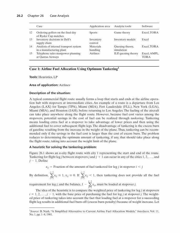
Figure 26.1 shows an n-city flight route with city 1 representing the start and end of the route.Tankering for flight leg j between stopovers j and can occur in any of the cities and
Define
By definition, If then tankering does not provide all the fuel
requirement for leg j, and the balance, must be loaded at stopover j.
The idea of the heuristic is to compare the weighted price of tankering for leg j at stopoverswith the base price of purchasing the fuel for leg j at stopover j. The weight-
ed price of tankering takes into account the fact that loading fuel at a stopover for a succeedingflight leg results in additional fuel burn-off (excess burn penalty) because of weight increase. Let
i = 1, 2, Á , j - 1,
1 - aj - 1
i = 1xij,
aj - 1
i = 1xij 6 1,a
j - 1
i = 1xij … 1, xij Ú 0.
xij = Fraction of the amount of fuel tankered for leg j in stopover i 6 j
j - 1.1, 2, Á ,j + 1
M26_TAHA5937_09_SE_C26.QXD 7/26/10 9:27 PM Page 26.2
Case 1: Airline Fuel Allocation Using Optimum Tankering 26.3
1 2 j j 1 n 1 n……
leg j
FIGURE 26.1
An n-stopover flight route
The weighted price, can be computed from the formula
Let
The heuristic rule recommends tankering at station for leg j if
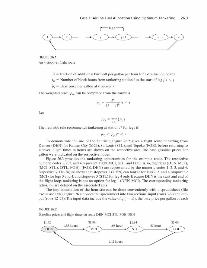
To demonstrate the use of the heuristic, Figure 26.2 gives a flight route departing fromDenver (DEN) for Kansas City (MCI), St. Louis (STL), and Topeka (FOE), before returning toDenver. Flight times in hours are shown on the respective arcs. The base gasoline prices pergallon were indicated on the respective nodes.
Figure 26.3 provides the tankering opportunities for the example route. The respectivenumeric codes 1, 2, 3, and 4 represent DEN, MCI, STL, and FOE. Also, flightlegs (DEN, MCI),(MCI, STL), (STL, FOE), (FOE, DEN) are represented by the numeric codes 1, 2, 3, and 4,respectively. The figure shows that stopover 1 (DEN) can tanker for legs 2, 3, and 4, stopover 2(MCI) for legs 3 and 4, and stopover 3 (STL) for leg 4 only. Because DEN is the start and end ofthe flight loop, tankering is not an option for leg 1 (DEN, MCI). The corresponding tankeringratios, are defined on the associated arcs.
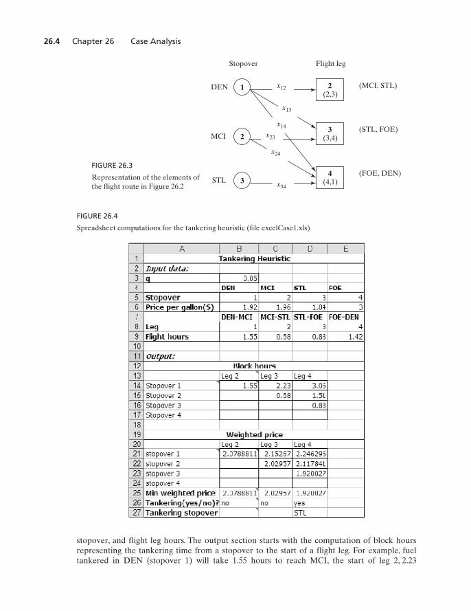
The implementation of the heuristic can be done conveniently with a spreadsheet (fileexcelCase1.xls). Figure 26.4 divides the spreadsheet into two sections: input (rows 3–9) and out-put (rows 12–27). The input data include the value of the base price per gallon at eachq 1= .052,
xij,
pi…j 6 pN j, i* 6 j
i*
pi…j = mini 6 j5pij6
pij =
pN i
11 - q2tij
, i 6 j
pij,
pN j = Base price per gallon at stopover j
tij = Number of block hours from tankering station i to the start of leg j, i 6 j
q = fraction of additional burn-off per gallon per hour for extra fuel on board
DEN MCI STL FOE
00.3$48.1$69.1$29.1$ruoh 86.sruoh 55.1
1.42 hours
.83 hour
FIGURE 26.2
Gasoline prices and flight times on route DEN-MCI-STL-FOE-DEN
M26_TAHA5937_09_SE_C26.QXD 7/26/10 9:27 PM Page 26.3
26.4 Chapter 26 Case Analysis
1
2
3
2(2,3)
3(3,4)
4(4,1)
x12
x13
x14
x23
x24
x34
Stopover Flight leg
DEN
MCI
STL
(MCI, STL)
(STL, FOE)
(FOE, DEN)FIGURE 26.3
Representation of the elements ofthe flight route in Figure 26.2
FIGURE 26.4
Spreadsheet computations for the tankering heuristic (file excelCase1.xls)
stopover, and flight leg hours. The output section starts with the computation of block hoursrepresenting the tankering time from a stopover to the start of a flight leg. For example, fueltankered in DEN (stopover 1) will take 1.55 hours to reach MCI, the start of leg 2, 2.23
M26_TAHA5937_09_SE_C26.QXD 7/26/10 9:27 PM Page 26.4
Case 1: Airline Fuel Allocation Using Optimum Tankering 26.5
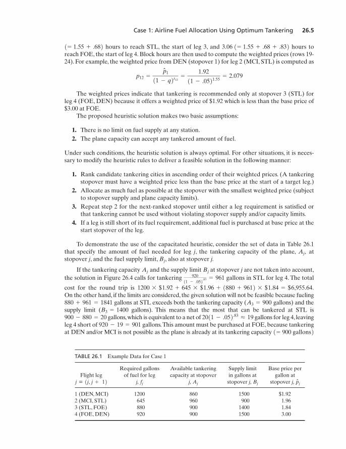
TABLE 26.1 Example Data for Case 1
Required gallons Available tankering Supply limit Base price perFlight leg of fuel for leg capacity at stopover in gallons at gallon at
j, j, stopover j, stopover j,
1 (DEN, MCI) 1200 860 1500 $1.922 (MCI, STL) 645 960 900 1.963 (STL, FOE) 880 900 1400 1.844 (FOE, DEN) 920 900 1500 3.00
pN jBjAjfjj K 1j, j + 12
hours to reach STL, the start of leg 3, and hours toreach FOE, the start of leg 4. Block hours are then used to compute the weighted prices (rows 19-24). For example, the weighted price from DEN (stopover 1) for leg 2 (MCI, STL) is computed as
The weighted prices indicate that tankering is recommended only at stopover 3 (STL) forleg 4 (FOE, DEN) because it offers a weighted price of $1.92 which is less than the base price of$3.00 at FOE.
The proposed heuristic solution makes two basic assumptions:
1. There is no limit on fuel supply at any station.2. The plane capacity can accept any tankered amount of fuel.
Under such conditions, the heuristic solution is always optimal. For other situations, it is neces-sary to modify the heuristic rules to deliver a feasible solution in the following manner:
1. Rank candidate tankering cities in ascending order of their weighted prices. (A tankeringstopover must have a weighted price less than the base price at the start of a target leg.)
2. Allocate as much fuel as possible at the stopover with the smallest weighted price (subjectto stopover supply and plane capacity limits).
3. Repeat step 2 for the next-ranked stopover until either a leg requirement is satisfied orthat tankering cannot be used without violating stopover supply and/or capacity limits.
4. If a leg is still short of its fuel requirement, additional fuel is purchased at base price at thestart stopover of the leg.
To demonstrate the use of the capacitated heuristic, consider the set of data in Table 26.1that specify the amount of fuel needed for leg j, the tankering capacity of the plane, atstopover j, and the fuel supply limit, also at stopover j.
If the tankering capacity and the supply limit at stopover j are not taken into account,the solution in Figure 26.4 calls for tankering gallons in STL for leg 4. The total
cost for the round trip is On the other hand, if the limits are considered, the given solution will not be feasible because fueling
gallons at STL exceeds both the tankering capacity ( gallons) and thesupply limit ( gallons). This means that the most that can be tankered at STL is
gallons, which is equivalent to a net of gallons for leg 4, leavingleg 4 short of gallons.This amount must be purchased at FOE, because tankeringat DEN and/or MCI is not possible as the plane is already at its tankering capacity 1= 900 gallons2
920 - 19 = 9012011 - .052.83
L 19900 - 880 = 20B3 = 1400
A3 = 900880 + 961 = 1841
1200 * $1.92 + 645 * $1.96 + 1880 + 9612 * $1.84 = $6,955.64.
92011 - .052.83 = 961
BjAj
Bj,Aj,
p12 =
pN 1
11 - q2t12=
1.92
11 - .0521.55= 2.079
3.06 1= 1.55 + .68 + .8321= 1.55 + .682
M26_TAHA5937_09_SE_C26.QXD 7/26/10 9:27 PM Page 26.5
26.6 Chapter 26 Case Analysis
in STL. The associated fuel cost for the tour thus equals an increase of
(or about 14%) over the cost of uncapacitated solution.
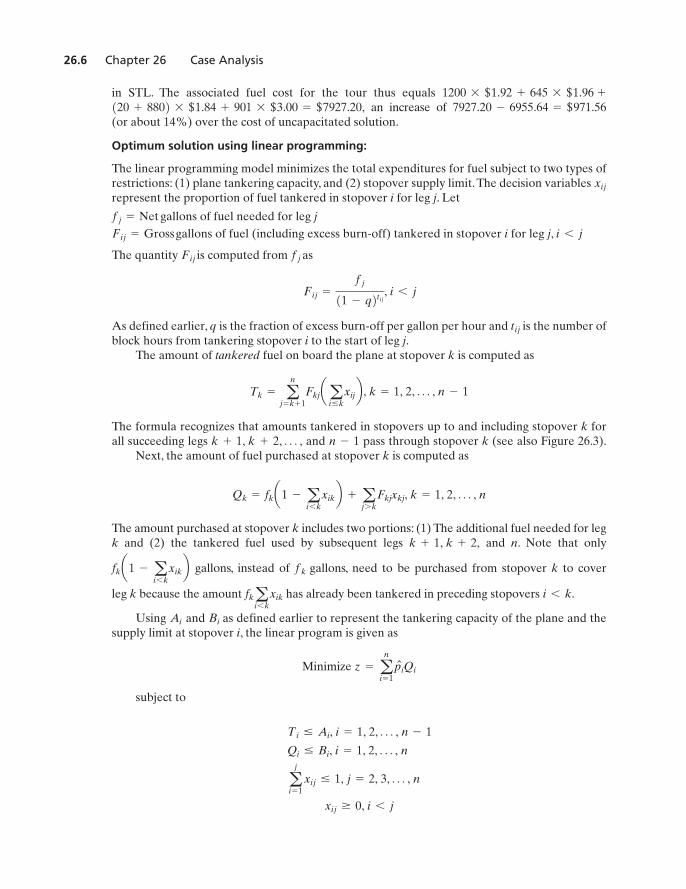
Optimum solution using linear programming:
The linear programming model minimizes the total expenditures for fuel subject to two types ofrestrictions: (1) plane tankering capacity, and (2) stopover supply limit.The decision variables represent the proportion of fuel tankered in stopover i for leg j. Let
gallons of fuel needed for leg jgallons of fuel (including excess burn-off) tankered in stopover i for leg j,
The quantity is computed from as
As defined earlier, q is the fraction of excess burn-off per gallon per hour and is the number ofblock hours from tankering stopover i to the start of leg j.
The amount of tankered fuel on board the plane at stopover k is computed as
The formula recognizes that amounts tankered in stopovers up to and including stopover k forall succeeding legs and pass through stopover k (see also Figure 26.3).
Next, the amount of fuel purchased at stopover k is computed as
The amount purchased at stopover k includes two portions: (1) The additional fuel needed for legk and (2) the tankered fuel used by subsequent legs and n. Note that only
gallons, instead of gallons, need to be purchased from stopover k to cover
leg k because the amount has already been tankered in preceding stopovers
Using and as defined earlier to represent the tankering capacity of the plane and thesupply limit at stopover i, the linear program is given as
subject to
xij Ú 0, i 6 j
aj
i = 1xij … 1, j = 2, 3, Á , n
Qi … Bi, i = 1, 2, Á , n
Ti … Ai, i = 1, 2, Á , n - 1
Minimize z = an
i = 1pNiQi
BiAi
i 6 k.fkai 6 k
xik
fkfka1 - ai 6 k
xikbk + 1, k + 2,
Qk = fka1 - ai 6 k
xikb + aj 7 k
Fkjxkj, k = 1, 2, Á , n
n - 1k + 1, k + 2, Á ,
Tk = an
j = k + 1Fkjaa
i … kxijb , k = 1, 2, Á , n - 1
tij
Fij =
fj
11 - q2tij, i 6 j
fjFij
i 6 jFij = Grossfj = Net
xij
7927.20 - 6955.64 = $971.56120 + 8802 * $1.84 + 901 * $3.00 = $7927.20,1200 * $1.92 + 645 * $1.96 +
M26_TAHA5937_09_SE_C26.QXD 7/26/10 9:27 PM Page 26.6

Case 1: Airline Fuel Allocation Using Optimum Tankering 26.7
The model is solved by substituting for and in terms of as given previously. Note that inthe third set of constraints the use of inequality instead of strict equality allows for thepossibility of no tankering for leg j.
The data of the heuristic example in Table 26.1 will be used to demonstrate the use of thelinear programming model. The first step is to compute using and as shown in Table 26.2.All values have been raised to the next integer value for convenience. To illustrate the computa-tions, we have
Thus, we get
The complete linear program is thus given as
subject to
Q4 + 920x14 + 920x24 + 920x34 = 920
Q3 + 880x13 + 880x23 - 961x34 = 880
Q2 + 645x12 - 912x23 - 995x24 = 645
Q1 - 699x12 - 987x13 - 1077x14 = 1200
961x14 + 961x24 + 961x34 … 900
912x13 + 912x23 + 995x14 + 995x24 … 960
699x12 + 987x13 + 1077x14 … 860
Q1 … 1500, Q2 … 900, Q3 … 1400, Q4 … 1500
Minimize z = 1.92Q1 + 1.96Q2 + 1.84Q3 + 3.00Q4
Q4 = 92011 - x14 - x24 - x342 Q3 = 88011 - x13 - x232 + 961x34
Q2 = 64511 - x122 + 912x23 + 995x24
Q1 = 1200 + 699x12 + 987x13 + 1077x14
T3 = 9611x14 + x24 + x342 T2 = 9121x13 + x232 + 9951x14 + x242 T1 = 699x12 + 987x13 + 1077x14
F12 =
f2
11 - q2t12=
645
11 - .0521.55= 698.37 L 699 gallons
tijfjFij
1…2xijQiTi
TABLE 26.2 Computation of using and
i
1 699 987 10772 912 9953 961
j = 4j = 3j = 2
Fij
tijfj
Fij
M26_TAHA5937_09_SE_C26.QXD 7/26/10 9:27 PM Page 26.7
26.8 Chapter 26 Case Analysis
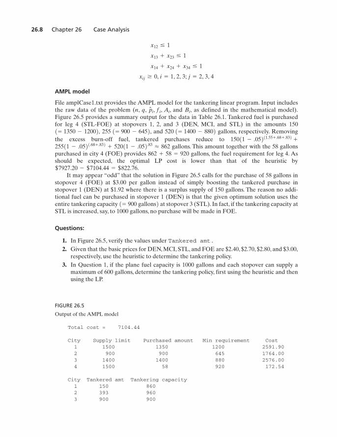
AMPL model
File amplCase1.txt provides the AMPL model for the tankering linear program. Input includesthe raw data of the problem (n, q, and as defined in the mathematical model).Figure 26.5 provides a summary output for the data in Table 26.1. Tankered fuel is purchasedfor leg 4 (STL-FOE) at stopovers 1, 2, and 3 (DEN, MCI, and STL) in the amounts
and gallons, respectively. Removingthe excess burn-off fuel, tankered purchases reduce to
gallons. This amount together with the 58 gallonspurchased in city 4 (FOE) provides gallons, the fuel requirement for leg 4. Asshould be expected, the optimal LP cost is lower than that of the heuristic by
It may appear “odd” that the solution in Figure 26.5 calls for the purchase of 58 gallons instopover 4 (FOE) at $3.00 per gallon instead of simply boosting the tankered purchase instopover 1 (DEN) at $1.92 where there is a surplus supply of 150 gallons. The reason no addi-tional fuel can be purchased in stopover 1 (DEN) is that the given optimum solution uses theentire tankering capacity at stopover 3 (STL). In fact, if the tankering capacity atSTL is increased, say, to 1000 gallons, no purchase will be made in FOE.
Questions:
1. In Figure 26.5, verify the values under Tankered amt.2. Given that the basic prices for DEN, MCI, STL, and FOE are $2.40, $2.70, $2.80, and $3.00,
respectively, use the heuristic to determine the tankering policy.3. In Question 1, if the plane fuel capacity is 1000 gallons and each stopover can supply a
maximum of 600 gallons, determine the tankering policy, first using the heuristic and thenusing the LP.
1= 900 gallons2
$7927.20 - $7104.44 = $822.76.
862 + 58 = 92025511 - .0521.68 + .832
+ 52011 - .052.83L 862
15011 - .05211.55 + .68 + .832 +520 1= 1400 - 8802255 1= 900 - 6452,1= 1350 - 12002,
150
Bi,pN i, fi, Ai,
xij Ú 0, i = 1, 2, 3; j = 2, 3, 4
x14 + x24 + x34 … 1
x13 + x23 … 1
x12 … 1
Total cost = 7104.44
City Supply limit Purchased amount Min requirement Cost1 1500 1350 1200 2591.902 900 900 645 1764.003 1400 1400 880 2576.004 1500 58 920 172.54
City Tankered amt Tankering capacity1 150 8602 393 9603 900 900
FIGURE 26.5
Output of the AMPL model
M26_TAHA5937_09_SE_C26.QXD 7/26/10 9:27 PM Page 26.8
Case 2: Optimization of Heart Valves Production 26.9
2Source: S.S. Hilal and W. Erikson,“Matching Supplies to Save Lives: Linear Programming the Production ofHeart Valves,” Interfaces, Vol. 11, No. 6, pp. 48–55, 1981.
4. Show that if the tankering capacity at stopover 3 (STL) is increased from 900 to 1000gallons, no purchase is made in stopover 4 (FOE) and the purchase in stopover 1 (MCI) isincreased to meet the fuel requirement for leg 4.
Case 2: Optimization of Heart Valves Production2
Tool: LP
Area of application: Bioprostheses (production planning)
Description of the situation:
Biological heart valves are bioprostheses manufactured from porcine hearts for human implan-tation. Replacement valves needed by the human population come in different sizes. On thesupply side, porcine hearts cannot be “produced” to specific sizes. Moreover, the exact size of amanufactured valve cannot be determined until the biological component of pig heart has beenprocessed. As a result, some needed sizes may be overstocked and others may be understocked.
Raw hearts are provided by several suppliers in six to eight sizes, usually in differentproportions depending on how the animals are raised. The distribution of sizes in each shipmentis expressed in the form of a histogram. Porcine specialists work with suppliers to ensure distri-bution stability as much as possible. In this manner, the manufacturer can have a reasonablyreliable estimate of the number of units of each size in each shipment.The selection of the mix ofsuppliers and the size of their shipments is thus crucial in reducing mismatches between supplyand demand.
LP model:
Let
Lj = Minimum monthly supply vendor j is willing to provide, j = 1, 2, Á , n
Hj = Maximum monthly supply vendor j can provide, j = 1, 2, Á , n
Di = Average monthly demand for valves of size i
= am
i = 1cipij, j = 1, 2, Á , n
cj = Average cost from supplier j
ci = Purchasing and processing cost of a raw heart of size i, i = 1, 2, Á , m
i = 1, 2, Á , m, j = 1, 2, Á , n, ami = 1 pij = 1, j = 1, 2, Á , n
pij = Proportion of raw valves of size i supplied by vendor j, 0 6 pij 6 1,
n = Number of suppliers
m = Number of valve sizes
M26_TAHA5937_09_SE_C26.QXD 7/26/10 9:27 PM Page 26.9
26.10 Chapter 26 Case Analysis
3There is one requirement about reading the data in array format from spreadsheet excelCase2.xls as used infile amplCase2.txt. The ODBC handler requires column headings in an Excel read table to be strings, whichmeans that a pure numeric heading is not acceptable. To get around this restriction, all column headings areconverted to strings using the Excel TEXT function. Thus, the heading 1 can be replaced with the formula
Copying this formula into succeeding columns will automatically convertthe numeric code into the desired strings.=TEXT1COLUMN1A12, “0”2.
The variables of the problem can be defined as
supply amount (number of raw hearts) by vendor
The LP model seeks to determine the amount from each supplier that will minimize the totalcost of purchasing and processing subject to demand and supply restrictions.
subject to
To be completely correct, the variables must be restricted to integer values. However, theparameters and are mere estimates and, hence, rounding the continuous solution to theclosest integer may not be a bad approximation in this case. This is particularly desirable forlarge problems, where imposing the integer restriction may result in unpredictable computationalexperiences.
AMPL Implementation:
Although the LP is quite simple as an AMPL application, the nature of the input data is some-what cumbersome. A convenient way to supply the data to this model is through a spreadsheet.File excelCase2.xls gives all the tables for the model and AMPL file amplCase2.txt shows howthe data involving 8 valve sizes and 12 suppliers are read from Excel tables.3
Analysis of the results:
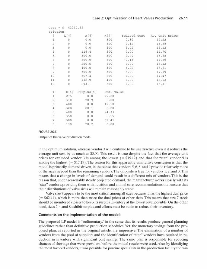
The output of the AMPL model for the data in excelCase2.xls is given in Figure 26.6. In the strictsense, the solution results cannot be used for scheduling purposes because the demand forheart valve i is based on expected value calculations. Thus, the solution willresult in some months showing surplus and others exhibiting shortage.
How useful then is the model? Actually, the results can be used effectively for planningpurposes. Specifically, the solution suggests grouping the vendors into three categories:
1. Vendors 1, 2, and 3 must be deleted from the list of suppliers because 2. Vendors 5, 6, 8, and 9 are crucial for satisfying demand because the solution requires these
vendors to supply all the hearts they can produce.3. The remaining vendors (4, 7, 10, 11, and 12) exhibit “moderate” importance from the
standpoint of satisfying demand because their maximum production capacity is not fullyutilized.
The given recommendations are further supported by the values of the reduced costs inFigure 26.6. Vendor 9 can raise its average unit prices by as much as $4.00 and still remain viable
x1 = x2 = x3 = 0.
xj, j = 1, 2, Á , n,Di
Dipij
xj
Lj … xj … Hj, j = 1, 2, Á , n
an
j = 1pijxj Ú Di, i = 1, 2, Á , m
Minimize z = an
j = 1cjxj
j, j = 1, 2, Á , nxj = Monthly
M26_TAHA5937_09_SE_C26.QXD 7/26/10 9:27 PM Page 26.10
Case 2: Optimization of Heart Valves Production 26.11
Cost = $ 42210.82solution:j L[j] x[j] H[j] reduced cost Av. unit price1 0 0.0 500 2.39 14.222 0 0.0 500 0.12 15.883 0 0.0 400 5.22 15.124 0 116.4 500 0.00 14.705 0 300.0 300 -0.49 16.686 0 500.0 500 -2.13 14.897 0 250.5 600 0.00 18.128 0 400.0 400 -6.22 16.619 0 300.0 300 -4.20 17.1910 0 357.4 500 -0.00 14.4711 0 112.9 400 0.00 15.6212 0 293.1 500 0.00 16.31
i D[i] Surplus[i] Dual value1 275 0.0 29.28 2 310 28.9 0.00 3 400 0.0 19.18 4 320 88.1 0.00 5 400 0.0 24.33 6 350 0.0 8.55 7 300 0.0 62.41 8 130 28.2 0.00
FIGURE 26.6
Output of the valve production model
in the optimum solution, whereas vendor 3 will continue to be unattractive even if it reduces theaverage unit cost by as much as $5.00. This result is true despite the fact that the average unitprices for excluded vendor 3 is among the lowest and that for “star” vendor 9 isamong the highest The reason for this apparently unintuitive conclusion is that themodel is primarily demand driven, in the sense that vendors 5, 6, 8, and 9 provide relatively moreof the sizes needed than the remaining vendors. The opposite is true for vendors 1, 2, and 3. Thismeans that a change in levels of demand could result in a different mix of vendors. This is thereason that, under reasonably steady projected demand, the manufacturer works closely with its“star” vendors, providing them with nutrition and animal care recommendations that ensure thattheir distributions of valve sizes will remain reasonably stable.
Valve size 7 appears to be the most critical among all sizes because it has the highest dual pricewhich is more than twice the dual prices of other sizes. This means that size 7 stock
should be monitored closely to keep its surplus inventory at the lowest level possible. On the otherhand, sizes 2, 4, and 8 exhibit surplus, and efforts must be made to reduce their inventory.
Comments on the implementation of the model:
The proposed LP model is “rudimentary,” in the sense that its results produce general planningguidelines rather than definitive production schedules. Yet, the monetary savings from the pro-posed plan, as reported in the original article, are impressive. The elimination of a number ofvendors from the pool of suppliers and the identification of “star” vendors have resulted in re-duction in inventory with significant cost savings. The same plan is responsible for reducingchances of shortage that were prevalent before the model results were used. Also, by identifyingthe most favored vendors, it was possible for porcine specialists in the production facility to train
1= $62.412,
1= $17.192.1= $15.122
M26_TAHA5937_09_SE_C26.QXD 7/26/10 9:27 PM Page 26.11
26.12 Chapter 26 Case Analysis
4Source: A.T. Ernst, R.G.J. Mills, and P. Welgama, “Scheduling Appointments at Trade Events for theAustralian Tourist Commission,” Interfaces, Vol. 33, No. 3, pp. 12–23, 2003.
the workers in the slaughterhouses of these vendors to provide well-isolated and well-trimmedhearts. This, in turn, has lead to streamlining production at the production facility.
Questions:
1. If the demands for the respective 8 sizes are 300, 200, 350, 450, 500, 200, 250, and 180 valves,find the new solution and compare it with the one given in the case analysis.
2. Suppose that vendor 3 is already under contract to supply 400 hearts for next year and thatthrough special diet it can alter the proportion of heart sizes it provides. What should bethe ideal proportion of sizes supplier 3 should provide?
Case 3: Scheduling Appointments at Australian Tourist Commission Trade Events4
Tools: Assignment model, heuristics
Area of application: Tourism
Description of the situation:
The Australian Tourist Commission (ATC) organizes trade events around the world to provide aforum for Australian sellers to meet international buyers of tourism products that include accom-modation, tours, transport, and others. During these events, sellers are stationed in booths andare visited by buyers according to pre-scheduled appointments. Because of the limited time slotsavailable in each event and the fact that the number of buyers and sellers can be quite large (onesuch event held in Melbourne in 1997 attracted 620 sellers and 700 buyers), ATC attempts toschedule the seller-buyer appointments in advance of the event in a manner that maximizes thepreferences. The idea is to match mutual interests to produce the most effective use of the limit-ed time slots available during the event.
Analysis:
The problem is viewed as a three-dimensional assignment model representing the buyers, the sell-ers, and the scheduled time slots. For an event with m buyers, n sellers, and T time slots, define
The associated assignment model can be expressed as
subject to
an
j = 1 xijt … 1, i = 1, 2, Á , m, t = 1, 2, Á , T
am
i = 1 xijt … 1, j = 1, 2, Á , n, t = 1, 2, Á , T
Maximize z = am
i = 1 a
n
j = 1 cijaa
T
t = 1xijtb
cij = A score representing the mutual preferences of buyer i and seller j
xijt = e1, if buyer i meets with seller j in period t0, otherwise
M26_TAHA5937_09_SE_C26.QXD 7/26/10 9:27 PM Page 26.12
Case 3: Scheduling Appointments at Australian Tourist Commission Trade Events 26.13
The model expresses the basic restrictions of an assignment model: Each buyer or seller canmeet at most one person per session and a specific buyer-seller meeting can take place in at mostone session. In the objective function, the coefficients representing the buyer-seller prefer-ences for meetings are not session dependent, because it is assumed that buyers and sellers areindifferent to the session time.
How are the coefficients determined? Following the registration of all buyers and sellers,each seller provides ATC with a prioritized list of buyers whom the seller wants to see. A similarlist is demanded of each buyer with respect to sellers. The list assigns the value 1 to the topchoice, with higher values implying lower preferences. These lists need not be exhaustive, in thesense that sellers and buyers are free to express interest in meeting with some but not all regis-tered counterparts. For example, in a list with 100 sellers, a buyer may seek meetings with 10 sell-ers only, in which case the expressed preferences will be for the selected sellers.
The raw data gathered from the buyers/sellers list may then be expressed algebraically as
From these definitions, the objective coefficients can be calculated as
The logic behind these formulas is that a smaller value of means a higher value of and,hence, a higher score assigned to a requested meeting between buyer i and seller j.A similar inter-pretation is given to the score for seller j’s requested meeting with buyer i. Both scores arenormalized to values between 0 and 1 by dividing them by B and S, respectively, and then areweighted by and to reflect the relative importance of the buyer and seller preferences,
Thus, values of less than .5 favor sellers’ preferences. Note that and indicate that no meetings are requested between buyer i and seller j.The quantity 1 appears in thetop three formulas of to give it a relatively larger preference than the case where no meetingsare requested (i.e., ).The normalization of the raw scores ensures that
Reliability of input data:
A crucial issue in the present situation is the reliability of the preference data provided by buy-ers and sellers.A preference collection tool is devised to guarantee that the following restrictionsare observed:
0 … cij 6 2.bij = sji = 0cij
sji = 0bij = 0a0 6 a 6 1.1 - aa
S - sji
1B - bij2bij
cij = g1 + aaB - bij
Bb + 11 - a2aS - sji
Sb , if bij Z 0 and sji Z 0
1 + aaB - bij
Bb , if bij Z 0 and sji = 0
1 + 11 - a2aS - sji
Sb , if bij = 0 and sji Z 0
0, if bij = sji = 0
cij
1 - a = relative weight of seller preferences.
a = relative weight of buyer preferences 1in calculating scores cij2, 0 6 a 6 1
S = maximum number of preferences elected by all sellers
B = maximum number of preferences elected by all buyers
sji = ranking assigned by seller j to a meeting with buyer i
bij = ranking assigned by buyer i to a meeting with seller j
1, 2, Á , 10
cij
cij
xijt = 10, 12 for all i, j, and t
aT
t = 1xijt … 1, i = 1, 2, Á , m, j = 1, 2, Á , n
M26_TAHA5937_09_SE_C26.QXD 7/26/10 9:27 PM Page 26.13
26.14 Chapter 26 Case Analysis
1. Lists of buyers and sellers are made available only after the registration deadline has passed.2. Only registered buyers and sellers can participate in the process.3. Participants’ preferences are kept confidential by ATC. They may not be seen or altered
by other participants.
Under these restrictions, an interactive internet site is created to allow participants to enter theirpreferences conveniently. More importantly, the design of the site ensures valid input data. Forexample, the system prevents a buyer from seeking more than one meeting with the same seller,and vice versa.
Solution of the problem:
The given assignment model is straightforward and can be solved by available commercial pack-ages. File amplCase3a.txt and file amplCase3b.txt provide two AMPL models for this situation.The data for the two models are given in a spreadsheet format (file excelCase3.xls). In the firstmodel, the spreadsheet is used to calculate the coefficients which are then used as input data.In the second model, the raw preference scores, and are the input data and the model itselfcalculates the coefficients The advantage of the second is that it allows computing the per-centages of buyer and seller satisfaction regarding their expressed preferences.
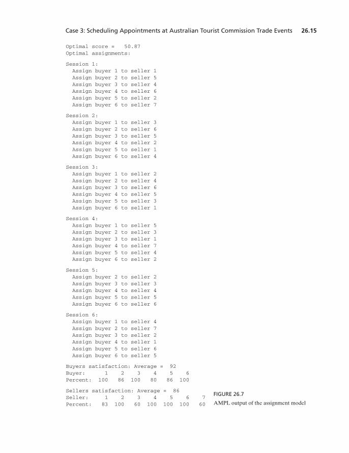
The output of model amplCase3b.txt for the data in file excelCase3.xls (6 buyers, 7 sellers,and 6 sessions) is given in Figure 26.7. It provides the assignment of buyers to sellers within eachsession as well as the percent satisfaction for each buyer and seller for a weight factor The results show high buyer and seller satisfactions (92% and 86%, respectively). If sell-er satisfaction will increase.
Practical considerations:
For the solution of the assignment model to be realistic, it must take into consideration the de-lays between successive appointments. Essentially, a buyer, once through with an appointment,will most likely have to move to another cubicle for the next appointment. A feasible schedulemust thus account for the transition time between successive appointments. The followingwalking constraints achieve this result:
The set represents the sellers buyer i cannot reach in period without experiencing unduedelay. The logic is that if buyer i has an appointment with seller j in period then thesame buyer may not schedule a next-period appointment with seller k who cannot bereached without delay (that is, ).We can reduce the number of such constraints by eliminat-ing period t that occurs at the end of a session block (e.g., coffee breaks, lunch break, and end of day).
The additional constraints increase the computational difficulty of the model considerably.In fact, the model may not be solvable as an integer linear program considering the computa-tional limitations of present-day IP algorithms. This is the reason a heuristic is needed to deter-mine a “good” solution for the problem.
The heuristic used to solve the new restricted model is summarized as follows:For each period t do
1. Set if the location of buyer i’s last meeting in period does not allow reachingseller j in period t.
2. Set if a meeting between i and j has been prescheduled.
3. Solve the resulting two-dimensional assignment model.
Next t
xijt = 0
t - 1xijt = 0
xi,k,t + 1 = 01t + 12
t1xijt = 12,t + 1Ji
xijt + akHJi
xi,k,t + 1 = 1, i = 1, Á , m, j = 1, Á , n, t = 1, Á , T
a 6 .5,a = .5.
cij.sji,bij
cij,
M26_TAHA5937_09_SE_C26.QXD 7/26/10 9:27 PM Page 26.14
Case 3: Scheduling Appointments at Australian Tourist Commission Trade Events 26.15
Optimal score = 50.87Optimal assignments:
Session 1:Assign buyer 1 to seller 1 Assign buyer 2 to seller 5 Assign buyer 3 to seller 4 Assign buyer 4 to seller 6 Assign buyer 5 to seller 2 Assign buyer 6 to seller 7
Session 2:Assign buyer 1 to seller 3 Assign buyer 2 to seller 6 Assign buyer 3 to seller 5 Assign buyer 4 to seller 2 Assign buyer 5 to seller 1 Assign buyer 6 to seller 4
Session 3:Assign buyer 1 to seller 2 Assign buyer 2 to seller 4 Assign buyer 3 to seller 6 Assign buyer 4 to seller 5 Assign buyer 5 to seller 3 Assign buyer 6 to seller 1
Session 4:Assign buyer 1 to seller 5 Assign buyer 2 to seller 3 Assign buyer 3 to seller 1 Assign buyer 4 to seller 7 Assign buyer 5 to seller 4 Assign buyer 6 to seller 2
Session 5:Assign buyer 2 to seller 2 Assign buyer 3 to seller 3 Assign buyer 4 to seller 4 Assign buyer 5 to seller 5 Assign buyer 6 to seller 6
Session 6:Assign buyer 1 to seller 4 Assign buyer 2 to seller 7 Assign buyer 3 to seller 2 Assign buyer 4 to seller 1 Assign buyer 5 to seller 6 Assign buyer 6 to seller 5
Buyers satisfaction: Average = 92Buyer: 1 2 3 4 5 6Percent: 100 86 100 80 86 100
Sellers satisfaction: Average = 86Seller: 1 2 3 4 5 6 7Percent: 83 100 60 100 100 100 60
FIGURE 26.7
AMPL output of the assignment model
M26_TAHA5937_09_SE_C26.QXD 7/26/10 9:27 PM Page 26.15
26.16 Chapter 26 Case Analysis
5Source: J.L. Huisingh, H.M Yamauchi, and R. Zimmerman, “Saving Federal Travel Dollars,” Interfaces,Vol. 31, No.5, pp. 13–23, 2001.
The quality of the heuristic solution can be measured by comparing its objective value (prefer-ence measure) with that of the original assignment model (with no walking constraints). Report-ed results show that for five separate events the gap between the two solutions was less than10%, indicating that the heuristic provides reliable solutions.
Of course, the devised solution does not guarantee that all preferences will be met becauseof the limit on the available number of time periods. Interestingly, the results recommended bythe heuristic show that at least 80% of the highest-priority meetings (with preference 1) are se-lected by the solution. This percentage declines almost linearly with the increase in expressedscores (higher score indicates lower preference).
Questions:
1. Suppose that the locations of booths preclude scheduling a buyer from holding meetingsin two successive sessions with sellers 1 and 3. Modify the AMPL model adding the walk-ing constraints and find the optimum solution.
2. Apply the heuristic to the situation in Question 1 and compare it with the optimum solution.
Case 4: Saving Federal Travel Dollars5
Tools: Shortest-route algorithm
Area of application: Business travel
Description of the situation:
U.S. Federal Government employees are required to attend development conferences and train-ing courses. Currently, the selection of the city hosting conferences and training events is donewithout consideration of incurred travel cost. Because federal employees are located in officesscattered around the United States, the location of the host city can impact travel cost, depend-ing on the number of participants and the locations from which they originate.
The General Services Administration (GSA) issues a yearly schedule of airfares that theGovernment contracts with different U.S. air carriers. This schedule provides fares for approxi-mately 5000 city-pair combinations in the contiguous 48 states. It also issues per-diem rates forall major cities and a flat daily rate for cities not included in the list. Participants using personalvehicles for travel receive a flat rate per mile.All rates are updated annually to reflect cost-of-livingincrease.The travel cost from a location to the host city is a direct function of the number of par-ticipants, the cost of travel to the host city, and the per-diem allowed for the host city.
The problem is concerned with the optimal location of host city for an event, given a speci-fied number of applicants from participating locations around the country.
Analysis:
The idea of the solution is simple:The host city must yield the lowest travel cost that includes (1)minimum transportation cost and (2) per-diem allowance for the host city. The determination ofthe transportation cost requires identifying the locations from which participants depart. It isreasonable to assume that for locations within 100 miles from the host city, participants use per-sonal vehicles as the selected mode of transportation. Others travel by air. The cost basis for air
M26_TAHA5937_09_SE_C26.QXD 7/26/10 9:27 PM Page 26.16
travelers consists of the sum of contracted airfares along the legs of the cheapest route to the hostcity. To determine such routes, it is necessary to identify the locations around the United Statesfrom which participants depart. Each such location is a possible host city candidate provided itoffers adequate airport and conference facilities. In the present case, 261 such locations with4640 contracted airport links are identified.
The determination of the cheapest airfare routes among the selected 261 locations with 4640air links is no simple task because a trip may involve multiple legs. Floyd’s algorithm (Section6.3.2) is ideal for determining such routes. The “distance” between two locations is representedby the contracted airfare provided by the government. Per the contract, the cost of the round tripticket then equals double the cost of the one-way trip.
To simplify the analysis, the study does not allow the use of car rentals at destinations. Theplausible assumption here is that the host hotel is in the vicinity of the airport, usually with freeshuttle service.
Per-diems cover lodging, meals, and incidental expenses. Participants arrive the day beforethe event starts. However, those arriving from locations within 100 miles arrive the morning ofthe first day of the event. All participants will check out of the hotel on the last day. Days of ar-rival and departure, government regulations for meals and incidental expenses allow only a 75%reimbursement of the full per-diem rate.
Numerical Example:
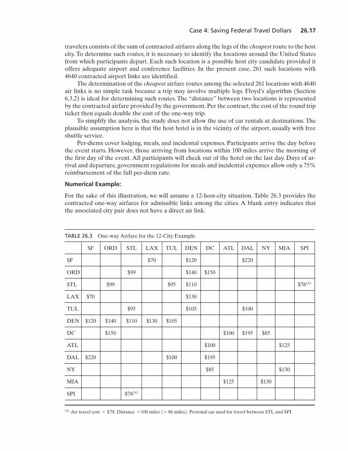
For the sake of this illustration, we will assume a 12-host-city situation. Table 26.3 provides thecontracted one-way airfares for admissible links among the cities. A blank entry indicates thatthe associated city pair does not have a direct air link.
Case 4: Saving Federal Travel Dollars 26.17
TABLE 26.3 One-way Airfare for the 12-City Example
SF ORD STL LAX TUL DEN DC ATL DAL NY MIA SPI
SF $70 $120 $220
ORD $99 $140 $150
STL $99 $95 $110 $78
LAX $70 $130
TUL $95 $105 $100
DEN $120 $140 $110 $130 $105
DC $150 $100 $195 $85
ATL $100 $125
DAL $220 $100 $195
NY $85 $130
MIA $125 $130
SPI $781a2
1a2
Air travel Personal car used for travel between STL and SPI.cost = $78. Distance 6 100 miles 1= 86 miles2.1a2
M26_TAHA5937_09_SE_C26.QXD 7/26/10 9:27 PM Page 26.17
26.18 Chapter 26 Case Analysis
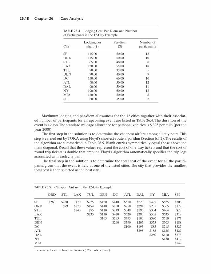
TABLE 26.5 Cheapest Airfare in the 12-City Example
ORD STL LAX TUL DEN DC ATL DAL NY MIA SPI
SF $260 $230 $70 $225 $120 $410 $510 $220 $495 $625 $308ORD $99 $270 $194 $140 $150 $250 $294 $235 $365 $177STL $240 $95 $110 $249 $349 $195 $334 $464 $28LAX $235 $130 $420 $520 $290 $505 $635 $318TUL $105 $295 $395 $100 $380 $510 $173DEN $290 $390 $205 $375 $505 $188DC $100 $195 $85 $215 $327ATL $295 $185 $125 $427DAL $280 $410 $273NY $130 $412MIA $542
Personal vehicle cost based on 86 miles (32.5 cents per mile).…
…
Maximum lodging and per-diem allowances for the 12 cities together with their associat-ed number of participants for an upcoming event are listed in Table 26.4. The duration of theevent is 4 days. The standard mileage allowance for personal vehicles is $.325 per mile (per theyear 2000).
The first step in the solution is to determine the cheapest airfare among all city pairs. Thisstep is carried out by TORA using Floyd’s shortest-route algorithm (Section 6.3.2).The results ofthe algorithm are summarized in Table 26.5. Blank entries symmetrically equal those above themain diagonal. Recall that these values represent the cost of one-way tickets and that the cost ofround trip tickets is double that amount. Floyd’s algorithm automatically specifies the trip legsassociated with each city pair.
The final step in the solution is to determine the total cost of the event for all the partici-pants, given that the event is held at one of the listed cities. The city that provides the smallesttotal cost is then selected as the host city.
TABLE 26.4 Lodging Cost, Per Diem, and Numberof Participants in the 12-City Example
Lodging per Per-diem Number ofCity night ($) ($) participants
SF 115.00 50.00 15ORD 115.00 50.00 10STL 85.00 48.00 8LAX 120.00 55.00 18TUL 70.00 35.00 5DEN 90.00 40.00 9DC 150.00 60.00 10ATL 90.00 50.00 12DAL 90.00 50.00 11NY 190.00 60.00 12MIA 120.00 50.00 8SPI 60.00 35.00 2
M26_TAHA5937_09_SE_C26.QXD 7/26/10 9:27 PM Page 26.18
Case 4: Saving Federal Travel Dollars 26.19
To demonstrate the computations, suppose that STL is the candidate host city. The associat-ed total cost is then computed as:
Note that because SPI is located 86 miles from STL, its participants drive per-sonal vehicles and arrive at STL the morning of the first day of the event. Thus, their per-diem isbased on days and their lodging is based on 3 nights only. Participants from STL receive per diem for days and no lodging. All other participants arrive at STL a day earlier, and theirper-diem is based on days and 4 nights of lodging.
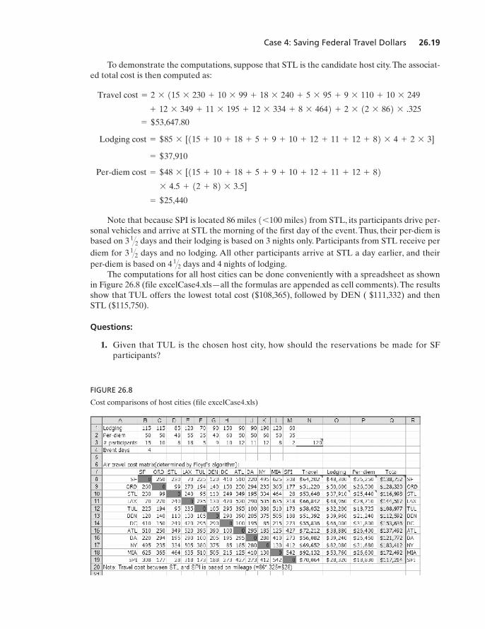
The computations for all host cities can be done conveniently with a spreadsheet as shownin Figure 26.8 (file excelCase4.xls—all the formulas are appended as cell comments). The resultsshow that TUL offers the lowest total cost ($108,365), followed by DEN ( $111,332) and thenSTL ($115,750).
Questions:
1. Given that TUL is the chosen host city, how should the reservations be made for SFparticipants?
4 1�2
3 1�2
3 1�2
16100 miles2 = $25,440
* 4.5 + 12 + 82 * 3.5]
Per-diem cost = $48 * [115 + 10 + 18 + 5 + 9 + 10 + 12 + 11 + 12 + 82 = $37,910
Lodging cost = $85 * [115 + 10 + 18 + 5 + 9 + 10 + 12 + 11 + 12 + 82 * 4 + 2 * 3]
= $53,647.80
+ 12 * 349 + 11 * 195 + 12 * 334 + 8 * 4642 + 2 * 12 * 862 * .325
Travel cost = 2 * 115 * 230 + 10 * 99 + 18 * 240 + 5 * 95 + 9 * 110 + 10 * 249
FIGURE 26.8
Cost comparisons of host cities (file excelCase4.xls)
M26_TAHA5937_09_SE_C26.QXD 7/26/10 9:27 PM Page 26.19
26.20 Chapter 26 Case Analysis
6Source: P. Choypeng, P. Puakpong, and R. Rosenthal, “Optimal Ship Routing and Personnel Assignment forNaval Recruitment in Thailand,” Interfaces, Vol. 16, No. 4, pp. 47–52, 1986.
2. Suppose that the following new air links are added to the list of admissible routes: ORD-NY ($150), LAX-MIA ($300), DEN-DAL ($110), ATL-NY ($150).Determine the host city.
Case 5: Optimal Ship Routing and Personnel Assignment for Naval Recruitment in Thailand6
Tools: Transportation model, ILP
Area of application: Transportation, routing
Description of the situation:
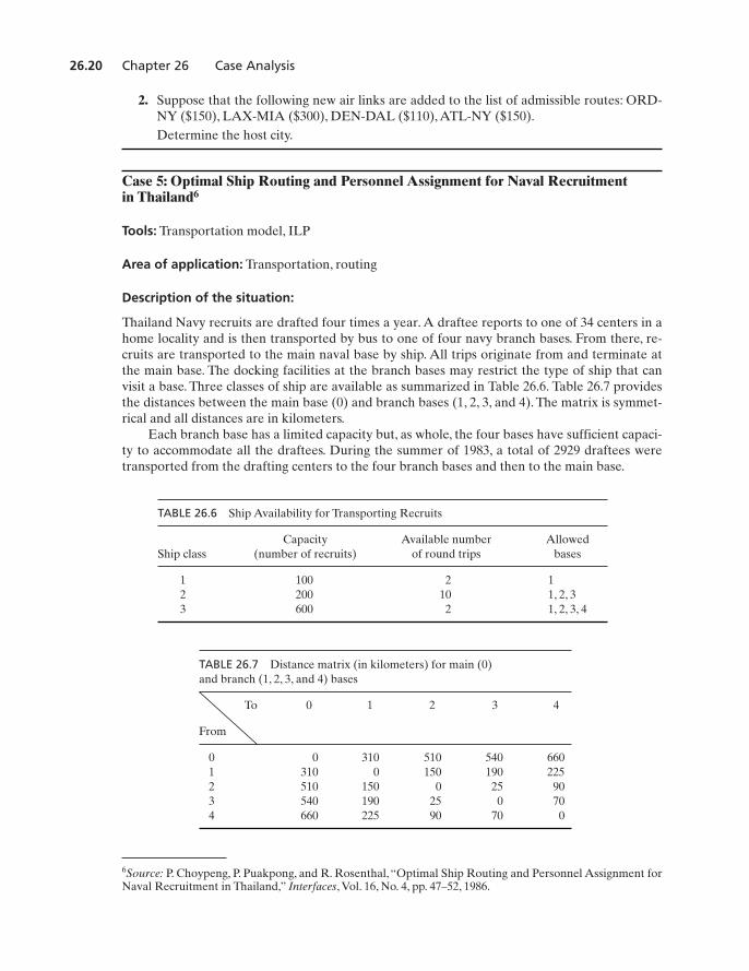
Thailand Navy recruits are drafted four times a year. A draftee reports to one of 34 centers in ahome locality and is then transported by bus to one of four navy branch bases. From there, re-cruits are transported to the main naval base by ship. All trips originate from and terminate atthe main base. The docking facilities at the branch bases may restrict the type of ship that canvisit a base. Three classes of ship are available as summarized in Table 26.6. Table 26.7 providesthe distances between the main base (0) and branch bases (1, 2, 3, and 4). The matrix is symmet-rical and all distances are in kilometers.
Each branch base has a limited capacity but, as whole, the four bases have sufficient capaci-ty to accommodate all the draftees. During the summer of 1983, a total of 2929 draftees weretransported from the drafting centers to the four branch bases and then to the main base.
TABLE 26.6 Ship Availability for Transporting Recruits
Capacity Available number AllowedShip class (number of recruits) of round trips bases
1 100 2 12 200 10 1, 2, 33 600 2 1, 2, 3, 4
TABLE 26.7 Distance matrix (in kilometers) for main (0) and branch (1, 2, 3, and 4) bases
To 0 1 2 3 4
From
0 0 310 510 540 6601 310 0 150 190 2252 510 150 0 25 903 540 190 25 0 704 660 225 90 70 0
M26_TAHA5937_09_SE_C26.QXD 7/26/10 9:27 PM Page 26.20
Case 5: Optimal Ship Routing and Personnel Assignment for Naval Recruitment 26.21
Two problems arise concerning the transportation of the recruits:
1. How should the draftees be transported by bus from drafting centers to branch bases?2. How should the draftees be transported by ship from branch bases to the main base?
Model development:
The solution of the problem is done in two independent stages:
1. Stage 1 determines the optimal allocation of draftees from the recruiting centers to thebranch bases.
2. Stage 2 then uses the result of Stage 1 to determine the optimal transportation schedulesfrom the branches to the main base.
The first problem is a straightforward transportation model with 34 sources (drafting cen-ters) and 4 branch bases (destinations). For the purpose of the model, the “supply” at a source isthe number of recruits a center drafts. The “demand” at a destination equals the number ofdraftees a branch base can receive. In the present situation the total supply does not exceed thetotal demand.The unit transportation equals the cost of a bus trip divided by the number of seatson the bus. We can represent the transportation unit as a bus load rather than an individual re-cruit by dividing the number of recruits at a center by the number of seats available on a bus, andthen round up the result. For example, 500 recruits from a drafting center on a bus with 52 seatswill require 10 bus trips. The unit transportation cost in this case is the cost per bus trip.
Whether we use a recruit or a bus load as the transportation unit, both representations areapproximations. The use of a recruit as the transportation unit can deflate the total transporta-tion cost, because a partially full bus incurs the same cost as a full bus. On the other hand, the useof a bus load as a transportation unit can inflate both the number of recruits and the capacitiesof the branch bases. Either way, the bias in the solution is not pronounced, because it only resultsfrom treating one partial bus load as a full load. In this study, a recruit is used as the transporta-tion unit.
Let
The mathematical model is
subject to
The model will yield a feasible (integer) solution so long as an acceptable assumption in this situation.
am
i = 1ai … a
n
j = 1bj,
xij Ú 0, for all i and j
am
i = 1xij … bj, j = 1, 2, Á , n
an
j = 1xij Ú ai, i = 1, 2, Á , m
Minimize z = am
i = 1an
j = 1cijxij
bj = Capacity 1in number of recruits2 at branch base j
ai = Number of recruits at center i
cij = Transportation cost per recruit from recruiting center i to branch base j
xij = Number of draftees at recruiting center i transported to branch base j
M26_TAHA5937_09_SE_C26.QXD 7/26/10 9:27 PM Page 26.21
26.22 Chapter 26 Case Analysis
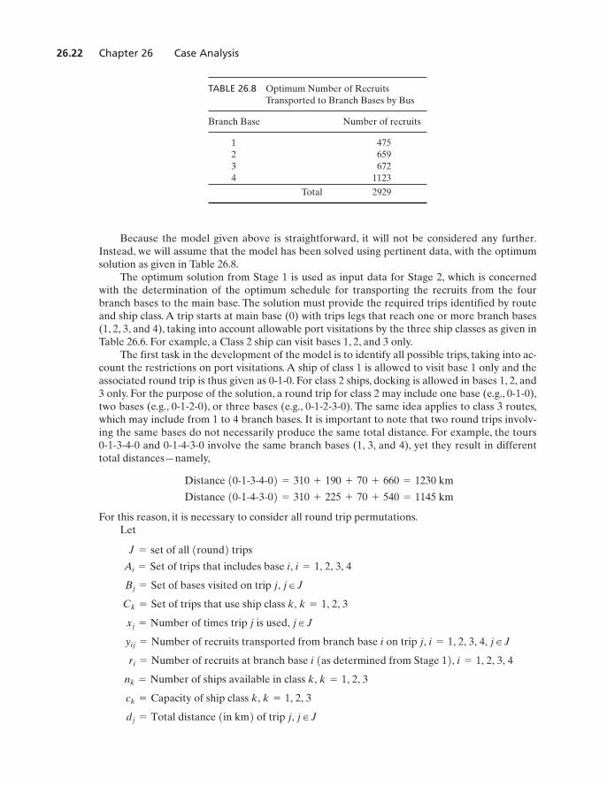
Because the model given above is straightforward, it will not be considered any further.Instead, we will assume that the model has been solved using pertinent data, with the optimumsolution as given in Table 26.8.
The optimum solution from Stage 1 is used as input data for Stage 2, which is concernedwith the determination of the optimum schedule for transporting the recruits from the fourbranch bases to the main base. The solution must provide the required trips identified by routeand ship class. A trip starts at main base (0) with trips legs that reach one or more branch bases(1, 2, 3, and 4), taking into account allowable port visitations by the three ship classes as given inTable 26.6. For example, a Class 2 ship can visit bases 1, 2, and 3 only.
The first task in the development of the model is to identify all possible trips, taking into ac-count the restrictions on port visitations. A ship of class 1 is allowed to visit base 1 only and theassociated round trip is thus given as 0-1-0. For class 2 ships, docking is allowed in bases 1, 2, and3 only. For the purpose of the solution, a round trip for class 2 may include one base (e.g., 0-1-0),two bases (e.g., 0-1-2-0), or three bases (e.g., 0-1-2-3-0). The same idea applies to class 3 routes,which may include from 1 to 4 branch bases. It is important to note that two round trips involv-ing the same bases do not necessarily produce the same total distance. For example, the tours0-1-3-4-0 and 0-1-4-3-0 involve the same branch bases (1, 3, and 4), yet they result in differenttotal distances—namely,
For this reason, it is necessary to consider all round trip permutations.Let
dj = Total distance 1in km2 of trip j, j H J
ck = Capacity of ship class k, k = 1, 2, 3
nk = Number of ships available in class k, k = 1, 2, 3
ri = Number of recruits at branch base i 1as determined from Stage 12, i = 1, 2, 3, 4
yij = Number of recruits transported from branch base i on trip j, i = 1, 2, 3, 4, j H J
xj = Number of times trip j is used, j H J
Ck = Set of trips that use ship class k, k = 1, 2, 3
Bj = Set of bases visited on trip j, j H J
Ai = Set of trips that includes base i, i = 1, 2, 3, 4
J = set of all 1round2 trips
Distance 10-1-4-3-02 = 310 + 225 + 70 + 540 = 1145 km
Distance 10-1-3-4-02 = 310 + 190 + 70 + 660 = 1230 km
TABLE 26.8 Optimum Number of Recruits Transported to Branch Bases by Bus
Branch Base Number of recruits
1 4752 6593 6724 1123
Total 2929
M26_TAHA5937_09_SE_C26.QXD 7/26/10 9:27 PM Page 26.22
Case 5: Optimal Ship Routing and Personnel Assignment for Naval Recruitment 26.23
The model for the ship-routing problem is
subject to
The first constraint ensures that all recruits will be transported.The second constraint recognizesthe capacity limitation of each ship class. The third constraint ensures that the number of roundtrips used in each class does not exceed availability.
AMPL solution:
File amplCase5.txt provides the AMPL model for the Stage 2 problem. The model automatical-ly generates all possible trips for each ship class and their distances. Perhaps the “trickiest” partof the model deals with the determination of the sets and as defined in the mathematicalmodel. These sets are determined by creating the matrix that mirrors the legs of the differenttrips by letting if base i is in trip j and otherwise. For example, if trip 30 is 0-1-4-3-0,then and Using the matrix the following substitu-tions in the constraint eliminate the need to determine the sets and explicitly:
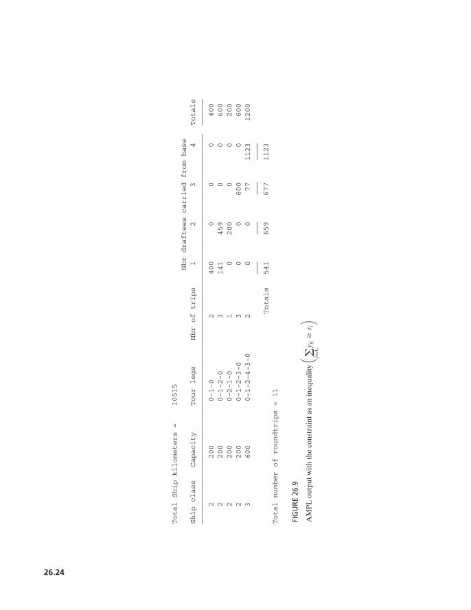
Figure 26.9 provides the output of the model using the data presented earlier. It identifiesthe trip and its associated ship class together with the number of times the trip is used. The num-ber of recruits from each base is also specified for each trip.The row and column totals affirm thefeasibility of the solution by showing that (1) ship capacity restrictions are met, and (2) the num-ber of recruits transported at least equals the number specified by the data of the problem (e.g.,at base 1, the solution guarantees that 541 recruits can be transported, which exceeds the actual475 recruits).
The reason the solution “inflates” the number of transported recruits is that we specified thefirst constraint as an inequality rather than an equation. This, however, does not mean that thesolution will use more “resources” than necessary.The inequality constraint simply allows the so-lution to “inflate” the number of recruits to make use of any excess capacity that may be avail-able on a ship. This is evident from the fact that the row total in Figure 26.9 exactly equals theship capacity multiplied by the number of trips.
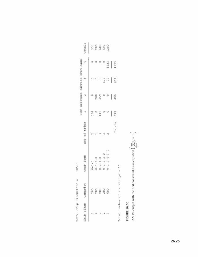
To show that the use of the inequality does not allow the use of more resources than is ab-solutely necessary, Figure 26.10 provides the output of the same model with the same data ex-cept that the inequality in the first constraint is replaced by an equation. In this case, the column
aiHBj
yij = a4
i = 1aijyij, j H Ck, k = 1, 2, 3
ajHAi
yij = ajHJ
aijyij, i = 1, 2, 3, 4
BjAi
7aij 7 ,a4,30 = 1.a1,30 = 1, a2,30 = 0, a3,30 = 1,aij = 0aij = 1
aij
BjAi
yij Ú 0 and integer, i = 1, 2, 3, 4, j H J
xj Ú 0 and integer, j H J
ajHCk
xj … nk, k = 1, 2, 3
aiHBj
yij … ckxj, j H Ck, k = 1, 2, 3
ajHAi
yij Ú ri, i = 1, 2, 3, 4
Minimize z = ajHJ
djxj
M26_TAHA5937_09_SE_C26.QXD 7/26/10 9:27 PM Page 26.23
26.24
Total Ship kilometers = 10515
Nbr draftees carried from base
Ship class Capacity Tour legs Nbr of trips 1 2 3 4 Totals
————————————————————————————————————————————————————————————————————————————————————————— ——————
2 200 0-1-0 2 400 0 0 0 400
2 200 0-1-2-0 3 141 459 0 0 600
2 200 0-2-1-0 1 0 200 0 0 200
2 200 0-1-2-3-0 3 0 0 600 0 600
3 600 0-1-2-4-3-0 2 0 0 77 1123 1200
Totals 541 659 677 1123
Total number of roundtrips = 11
FIG
UR
E 26
.9
AM
PL
out
put w
ith
the
cons
trai
nt a
s an
ineq
ualit
y a a jH
Aiy i
jÚ
r ib
M26_TAHA5937_09_SE_C26.QXD 7/26/10 9:27 PM Page 26.24
Total Ship kilometers = 10515
Nbr draftees carried from base
Ship class Capacity Tour legs Nbr of trips 1 2 3 4 Totals
—————————————————————————————————————————————————————————————————————————————————————————-
——————
2 200 0-1-0 2 334 0 0 0 334
2 200 0-1-2-0 1 0 200 0 0 200
2 200 0-2-1-0 3 141 459 0 0 600
2 200 0-1-2-3-0 3 0 0 595 0 595
3 600 0-1-2-4-3-0 2 0 0 77 1123 1200
Totals 475 659 672 1123
Total number of roundtrips = 11
FIG
UR
E 26
.10
AM
PL
out
put w
ith
the
firs
t con
stra
int a
s an
equ
atio
n a a jH
Aiy i
j=
r ib
26.25
M26_TAHA5937_09_SE_C26.QXD 7/26/10 9:27 PM Page 26.25
26.26 Chapter 26 Case Analysis
sums exactly equal the number of recruits at each base, whereas the row sums indicate that the“used” capacity on the ships can be less the total available capacity. For example, trip 0-1-0 car-ries 390 recruits from base 1, which is less than the maximum capacity of two trips of a class 2ship The fact remains that two trips will be made, exactly as the solution inFigure 26.9 specifies.
Computational considerations
Despite the fact that the two formulations (with inequality and equality constraints) produce thesame optimum solution, the computational experience with the two ILPs are different. In theequality constraint case, AMPL generated a total of 34,290 branch-and-bound nodes, which is70% more than the 20,690 nodes generated in the case of the inequality constraint.7 It wouldseem that the more restricted solution space should have resulted in a faster convergence of thebranch-and-bound algorithm because, in a way, it sets tighter limits on the feasible integer space.Unfortunately, no such rule can be recommended, as the (generally bizarre) behavior of thebranch-and-bound algorithm is also problem dependent.
Questions:
1. Consider the following round trips:Ship class 1: 0-1-0Ship class 2: 0-1-0, 0-3-2-0, 0-1-2-3-0, 0-2-3-0Ship class 3: 0-3-0, 0-1-4-3-2-0, 0-3-1-0, 0-4-2-1-0, 0-3-4-1-0(a) Given that these are the only trips allowed, develop the corresponding matrix.(b) Write down the explicit ILP for stage 2.
2. Suppose that there is a fixed cost of $5000 associated with each docking/undocking opera-tion at a port. Further, the operating costs per kilometer are $100, $120, and $150 for shipclasses 1, 2, and 3, respectively. Using the data in the case analysis, determine the optimaltransportation schedule from the four bases to the main base.
Case 6: Allocation of Operating Room Time in Mount Sinai Hospital8
Tools: ILP, GP
Area of application: Health care
Description of the situation:
The situation takes place in Canada, where health care insurance is mandatory and universal forall citizens. Funding, which is based on a combination of premiums and taxes, is controlled by theindividual provinces. Under this system, hospitals are advanced a fixed annual budget and eachprovince pays physicians retroactively using a fee-for-service funding mechanism. Local gov-ernments control the size of the health-care system by placing strict limits on hospital spending.The result is that the use of health resources, particularly operating rooms, must be controlledeffectively.
7aij 7
1= 2 * 200 = 4002.
7This experience is based on CPLEX 9.1.3.8Source: J.T. Blake and J. Donald, “Mount Sinai Hospital Uses Integer Programming to Allocate OperatingRoom Time,” Interfaces, Vol. 32, No. 2, pp. 63–73, 2002.
M26_TAHA5937_09_SE_C26.QXD 7/26/10 9:27 PM Page 26.26
Case 6: Allocation of Operating Room Time in Mount Sinai Hospital 26.27
TABLE 26.10 Weekly Demand for Operating Room Hours
Allowable limit ofDepartment Weekly target hours underallocated hours
Surgery 189.0 10.0Gynecology 117.4 10.0Ophthalmology 39.4 10.0Oral surgery 19.9 10.0Otolaryngology 26.3 10.0Emergency 5.4 3.0
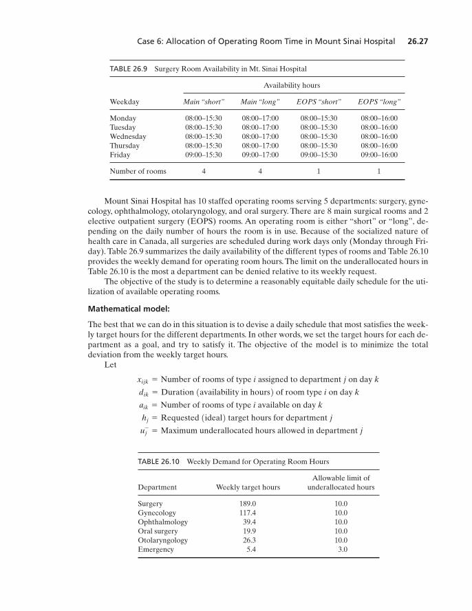
Mount Sinai Hospital has 10 staffed operating rooms serving 5 departments: surgery, gyne-cology, ophthalmology, otolaryngology, and oral surgery. There are 8 main surgical rooms and 2elective outpatient surgery (EOPS) rooms. An operating room is either “short” or “long”, de-pending on the daily number of hours the room is in use. Because of the socialized nature ofhealth care in Canada, all surgeries are scheduled during work days only (Monday through Fri-day). Table 26.9 summarizes the daily availability of the different types of rooms and Table 26.10provides the weekly demand for operating room hours. The limit on the underallocated hours inTable 26.10 is the most a department can be denied relative to its weekly request.
The objective of the study is to determine a reasonably equitable daily schedule for the uti-lization of available operating rooms.
Mathematical model:
The best that we can do in this situation is to devise a daily schedule that most satisfies the week-ly target hours for the different departments. In other words, we set the target hours for each de-partment as a goal, and try to satisfy it. The objective of the model is to minimize the totaldeviation from the weekly target hours.
Let
uj-
= Maximum underallocated hours allowed in department j
hj = Requested 1ideal2 target hours for department j
aik = Number of rooms of type i available on day k
dik = Duration 1availability in hours2 of room type i on day k
xijk = Number of rooms of type i assigned to department j on day k
TABLE 26.9 Surgery Room Availability in Mt. Sinai Hospital
Availability hours
Weekday Main “short” Main “long” EOPS “short” EOPS “long”
Monday 08:00–15:30 08:00–17:00 08:00–15:30 08:00–16:00Tuesday 08:00–15:30 08:00–17:00 08:00–15:30 08:00–16:00Wednesday 08:00–15:30 08:00–17:00 08:00–15:30 08:00–16:00Thursday 08:00–15:30 08:00–17:00 08:00–15:30 08:00–16:00Friday 09:00–15:30 09:00–17:00 09:00–15:30 09:00–16:00
Number of rooms 4 4 1 1
M26_TAHA5937_09_SE_C26.QXD 7/26/10 9:27 PM Page 26.27
26.28 Chapter 26 Case Analysis
The given situation involves 6 departments and 4 types of rooms. Thus, andFor a 5-day work week, the index k assumes the values 1 through 5.
The following integer-goal programming model represents the Mount Sinai Hospital sched-uling situation:
subject to
(1)
(2)
(3)
(4)
(5)
The logic of the model is that it may not be possible to satisfy the target hours for depart-ment j, Thus, the objective is to determine a schedule that minimizes possible“underallocation” of rooms to the different departments.To do this, the nonnegative variables and in constraint (1) represent the under- and over-allocation of hours relative to the target
for department j. The ratio measures the relative amount of underallocation to department j.Constraint (2) recognizes room availability limits. Constraint (3) is used to limit the amount bywhich a department is underallocated. The limits are user-specified.
Model results
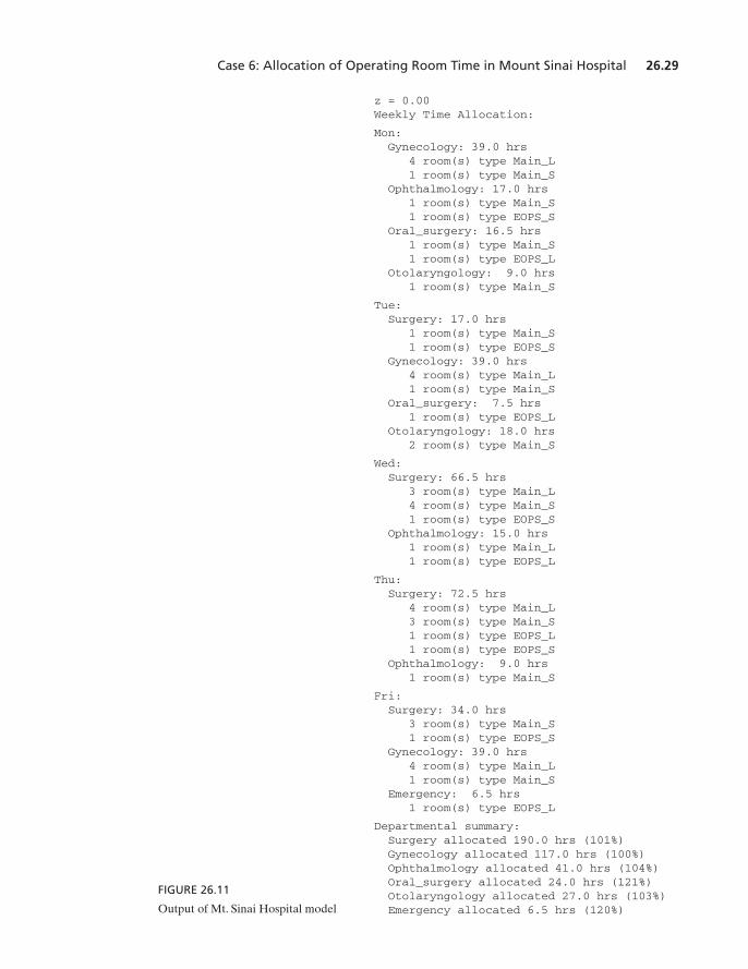
File amplCase6.txt gives the AMPL model of the problem. Figure 26.11 gives the solution for thedata provided in the statement of the problem. It shows that all goals are satisfied and itdetails the allocation of rooms (by type) to the different departments during the work week(Monday through Friday). Indeed, the departmental summary given at the bottom of the figureshows that the requests for 5 (out of 6) departments are oversatisfied. This happens to be thecase because there is abundance of resources for the week and the model does not try to mini-mize the overallocation of hours to the different departments. Actually, it makes no sense in thepresent model to try to do away with overallocation of hours, because the rooms are availableand might as well be apportioned to the different departments. In essence, the main concern isabout underallocation when available resources do not meet demand.
Computational experience:
In the model, the variable represents the number of allocated rooms. It must assume integervalues, and here lies a familiar problem that continues to plague integer programming computa-tions. The AMPL model executed rapidly with the set of data given in the description of theproblem. However, when the data representing target hours, were adjusted slightly (keepingall other data unchanged), the computational experience was totally different. First, the execu-tion time lasted more than one hour (as opposed to a few seconds with the initial set of data)and, after exploring more than 45 million branch-and-bound nodes, failed to produce a feasiblesolution, let alone the optimum.This experience appears to take place when the demand exceedsthe supply.Actually, the behavior of this ILP is unpredictable, because when the objective function
hj,
xijk
1z = 02
uj-
sj-
hj
hjsj+
sj-
j = 1, 2, Á , 6.hj
sj-, sj
+
Ú 0, for all j
xijk Ú 0 and integer for all i, j, and k
0 … sj-
… uj-, for all j
a6
j = 1xijk … aik, for all i and k
a4
i = 1a
5
k = 1dikxijk + sj
-
- sj+
= hj, for all j
Minimize z = a6
j = 1A 1
hjBsj
-
j = 1, 2, Á , 6.i = 1, 2, 3, 4
M26_TAHA5937_09_SE_C26.QXD 7/26/10 9:27 PM Page 26.28
Case 6: Allocation of Operating Room Time in Mount Sinai Hospital 26.29
z = 0.00 Weekly Time Allocation:
Mon:Gynecology: 39.0 hrs
4 room(s) type Main_L1 room(s) type Main_S
Ophthalmology: 17.0 hrs1 room(s) type Main_S1 room(s) type EOPS_S
Oral_surgery: 16.5 hrs1 room(s) type Main_S1 room(s) type EOPS_L
Otolaryngology: 9.0 hrs1 room(s) type Main_S
Tue:Surgery: 17.0 hrs
1 room(s) type Main_S1 room(s) type EOPS_S
Gynecology: 39.0 hrs4 room(s) type Main_L1 room(s) type Main_S
Oral_surgery: 7.5 hrs1 room(s) type EOPS_L
Otolaryngology: 18.0 hrs2 room(s) type Main_S
Wed:Surgery: 66.5 hrs
3 room(s) type Main_L4 room(s) type Main_S1 room(s) type EOPS_S
Ophthalmology: 15.0 hrs1 room(s) type Main_L1 room(s) type EOPS_L
Thu:Surgery: 72.5 hrs
4 room(s) type Main_L3 room(s) type Main_S1 room(s) type EOPS_L1 room(s) type EOPS_S
Ophthalmology: 9.0 hrs1 room(s) type Main_S
Fri:Surgery: 34.0 hrs
3 room(s) type Main_S1 room(s) type EOPS_S
Gynecology: 39.0 hrs4 room(s) type Main_L1 room(s) type Main_S
Emergency: 6.5 hrs1 room(s) type EOPS_L
Departmental summary:Surgery allocated 190.0 hrs (101%)Gynecology allocated 117.0 hrs (100%)Ophthalmology allocated 41.0 hrs (104%)Oral_surgery allocated 24.0 hrs (121%)Otolaryngology allocated 27.0 hrs (103%)Emergency allocated 6.5 hrs (120%)
FIGURE 26.11
Output of Mt. Sinai Hospital model
M26_TAHA5937_09_SE_C26.QXD 7/26/10 9:27 PM Page 26.29
26.30 Chapter 26 Case Analysis
9Source: H. Taha, “An Alternative Model for Optimizing Payloads of Building Glass at BFG,” South AfricanJournal of Industrial Engineering, Vol. 15, No. 1, pp. 31–43, 2003.
is changed to simply minimize the unweighted sum of all previously unsolvable cases aresolved instantly. The questions at the end of this case outline these computational experiences.
What courses of action are available for overcoming this problem? At first thought, thetemptation may be to drop the integer requirement and then round the resulting linear pro-gramming solution.This option will not work in this case because, in all likelihood, it will not pro-duce a feasible solution. Given that a specific number of hospital rooms are available, it is highlyunlikely that a trial-and-error rounded solution will meet room availability limits. This meansthat there is no alternative to imposing the integer condition.
One way to improve the chances for a successful execution of the integer model is to limitthe feasible ranges for the variables by taking into account the availability of other re-sources. For example, if the hospital has only two dental surgeons on a given day, no more thantwo rooms (of any type) can be assigned to that department on that day. Setting such boundsmay be effective in securing an optimal integer solution. Short of meeting this requirement, theonly remaining option is to devise a heuristic for the problem.
Question:
1. In amplCase6.txt,(a) Replace the current values of with
param h:= Surgery 190 Gynecology 122 Ophthalmology 41.4
Oral_surgery 20.9 Otolaryngology 25.3 Emergency 6.0;
Execute the model with the new data. You will notice that the model will execute forover one hour without finding a feasible solution.
(b) Using the original data of the model, change parameter a so that only 3 rooms ofMain_L are available during all five working days of the week. As in (a), AMPL failsto produce a solution.
(c) In both cases (a) and (b), replace the objective function with
minimize z: sum{j in departments}(sMinus[j])
which call for minimizing the sum of Now, execute the model and you will noticethat in both situations, the optimum is found instantly.
Case 7: Optimizing Trailer Payloads at PFG Building Glass9
Tools: ILP, static force (free-body diagram) calculations
Area of application: Transportation and distribution
Description of the situation:
PFG, a South African glass manufacturer, uses specially equipped (fifth-wheel) trailers to deliv-er packs of flat glass sheets to customers. Packs normally vary in both size and weight, and a singletrailer load may include different packs depending on received orders. Figure 26.12 illustrates atypical hauler-trailer rig with its axles located at points A, B, and C. Government regulations set
sj-.
hj
xijk
sj-,
M26_TAHA5937_09_SE_C26.QXD 7/26/10 9:27 PM Page 26.30
Case 7: Optimizing Trailer Payloads at PFG Building Glass 26.31
ABC
reliarTreluaH
FIGURE 26.12
Points A, B, and C of axle weights in hauler-trailer rig
maximum limits on axle weights. The actual positioning of the packs on the trailer is crucial indetermining these weights. Placing heavier packs toward the back of the trailer increases theload on axle A and placing them toward the front of the trailer shifts the load to axles B and C.The objective is to determine the location of a specific order of packs on the trailer bed that sat-isfies axle weight limits. Of course, the order mix may be such that axle weight limits will be ex-ceeded regardless of the positioning of packs. In such cases, the solution should provideinformation regarding excess weight on each axle to allow modifying the order mix and, hence,obtaining a new solution. This process is repeated until all weight limits are met.
The nature of the problem precludes minimizing the weight on each of the three axles, be-cause a reduction in the weight on one axle automatically increases the weight on another. Forthis reason, a realistic goal is to determine a “compromise” distribution of axle weights. Thispoint will be developed further after the details of the problem have been presented.
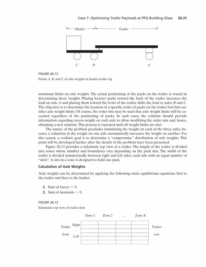
Figure 26.13 provides a schematic top view of a trailer. The length of the trailer is dividedinto zones whose number and boundaries vary depending on the pack mix. The width of thetrailer is divided symmetrically between right and left sides, each side with an equal number of“slots”. A slot in a zone is designed to hold one pack.
Calculation of Axle Weights
Axle weights can be determined by applying the following static equilibrium equations, first tothe trailer and then to the hauler:
1. Sum of 2. Sum of moments = 0.
forces = 0.
Zone 1 Zone 2 … Zone K
RightTrailer
frontLeft
Trailer
rear
FIGURE 26.13
Schematic top view of trailer slots
M26_TAHA5937_09_SE_C26.QXD 7/26/10 9:27 PM Page 26.31
26.32 Chapter 26 Case Analysis
d1
f1 f2 f3
fT
dT
dA
d2
RfA
d3
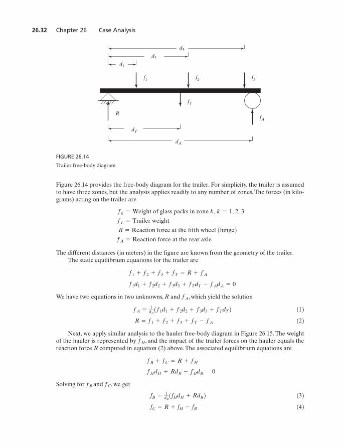
FIGURE 26.14
Trailer free-body diagram
Figure 26.14 provides the free-body diagram for the trailer. For simplicity, the trailer is assumedto have three zones, but the analysis applies readily to any number of zones. The forces (in kilo-grams) acting on the trailer are
The different distances (in meters) in the figure are known from the geometry of the trailer.The static equilibrium equations for the trailer are
We have two equations in two unknowns, R and which yield the solution
(1)
(2)
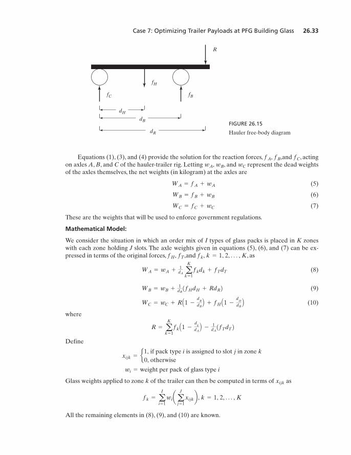
Next, we apply similar analysis to the hauler free-body diagram in Figure 26.15. The weightof the hauler is represented by and the impact of the trailer forces on the hauler equals thereaction force R computed in equation (2) above. The associated equilibrium equations are
Solving for and we get
(3)
(4) fC = R + fH - fB
fB =1
dB1fHdH + RdR2
fC,fB
fHdH + RdR - fBdB = 0
fB + fC = R + fH
fH,
R = f1 + f2 + f3 + fT - fA
fA =1
dA1f1d1 + f2d2 + f3d3 + fTdT2
fA,
f1d1 + f2d2 + f3d3 + fTdT - fAdA = 0
f1 + f2 + f3 + fT = R + fA
fA = Reaction force at the rear axle
R = Reaction force at the fifth wheel 1hinge2 fT = Trailer weight
fk = Weight of glass packs in zone k, k = 1, 2, 3
M26_TAHA5937_09_SE_C26.QXD 7/26/10 9:27 PM Page 26.32
Case 7: Optimizing Trailer Payloads at PFG Building Glass 26.33
Equations (1), (3), and (4) provide the solution for the reaction forces, and actingon axles A, B, and C of the hauler-trailer rig. Letting and represent the dead weightsof the axles themselves, the net weights (in kilogram) at the axles are
(5)
(6)
(7)
These are the weights that will be used to enforce government regulations.
Mathematical Model:
We consider the situation in which an order mix of I types of glass packs is placed in K zoneswith each zone holding J slots. The axle weights given in equations (5), (6), and (7) can be ex-pressed in terms of the original forces, and as
(8)
(9)
(10)
where
Define
Glass weights applied to zone k of the trailer can then be computed in terms of as
All the remaining elements in (8), (9), and (10) are known.
fk = aI
i = 1wiaa
J
j = 1xijkb , k = 1, 2, Á , K
xijk
wi = weight per pack of glass type i
xijk = e1, if pack type i is assigned to slot j in zone k0, otherwise
R = aK
k = 1fk A1 -
dk
dAB -
1dA1fTdT2
WC = wC + R A1 -
dR
dBB + fH A1 -
dH
dBB
WB = wB +1
dB1fHdH + RdR2
WA = wA +1
dA a K
k = 1
fkdk + fTdT
fk, k = 1, 2, Á , K,fH, fT,
WC = fC + wC
WB = fB + wB
WA = fA + wA
wCwA, wB,fC,fA, fB,
R
fBfC
fH
dH
dB
dR
FIGURE 26.15
Hauler free-body diagram
M26_TAHA5937_09_SE_C26.QXD 7/26/10 9:27 PM Page 26.33
26.34 Chapter 26 Case Analysis
Having expressed axle weights in terms of the variable we can now construct the opti-mization model.The main purpose of the model is to assign packs to slots such that the total axleweights, and remain within the government limits.We cannot just include these lim-its as simple constraints of the form and because the problemmay not have a feasible solution. Ideally, then, we would like to determine the values of thatwill reduce the individual axle weights as much as possible. If the resulting minimum weightsmeet government regulations, then the solution is feasible. Else, the size of the order mix must bereduced and a new solution attempted. The difficulty with this “idealized” solution is that thenature of the problem does not allow the minimization of individual axle weights because, as westated earlier, they are not independent, and a decrease in one axle load automatically increasesanother.
A formulation that comes close to minimizing the individual axle weights is to find a solu-tion that minimizes the largest of the axle weights. This formulation has the advantage of con-centrating on the most extreme of all three weights. Mathematically, the objective function isexpressed as
This function can be linearized readily by using the following standard substitution. Let
Then the objective function can be expressed as
subject to
We now turn our attention to the development of the constraints of the model. These con-straints deal with
1. At most one pack per slot is allowed.2. Zone weight limit cannot be exceeded.3. Number of packs (by type) to be loaded on trailer bed are limited by order mix.4. Axle weights should not exceed regulations.5. Packs are pushed toward the center of each zone to reduce trailer tipping.
The first four constraints are essential and must be included in the model. Constraint 5, thoughincluded in the model, is really not crucial because the entire glass weight in zone k is represent-ed by which is not a function of the width of the zone. Whatever the solution, then, the actualzone loading automatically moves the packs toward the center.
Define
LC = Allowable weight limit on axle C 1hauler front axle2 LB = Allowable weight limit on axle B 1hauler rear axle2 LA = Allowable weight limit on axle A 1trailer rear axle2 Lk = Glass load weight limit in zone k, k = 1, 2, Á , K
fk,
WC … y
WB … y
WA … y
Minimize z = y
y = max5WA, WB, WC6
Minimize z = max5WA, WB, WC6
xijk
WC … LCWA … LA, WB … LB,WC,WA, WB,
xijk,
M26_TAHA5937_09_SE_C26.QXD 7/26/10 9:27 PM Page 26.34
Case 7: Optimizing Trailer Payloads at PFG Building Glass 26.35
Constraints (1) through (5) are expressed mathematically as
(1)
(2)
(3)
(4a)
(4b)
(4c)
(5a)
(5b)
I and J, as defined previously, represent the number of glass types and the number of slots perzone.
Constraint (3) is not set as a strict equation to allow the model to load less than the ordersize, if necessary, to meet the regulations limit specified by constraint (4). However, because themodel objective function tries to minimize the maximum of axle weights, y, the obvious optimumsolution, given that constraint (3) is an inequality, is not to load any packs on the trailer bed. Toremedy the situation, the objective function is modified to allow loading as many packs as possi-ble without violating the regulations.
Define the nonnegative variable such that
(2a)
The idea is to force the slack variables to assume minimum values, which, inturn, requires loading the most packs allowed by constraint (3). The situation now is that weneed to minimize y as defined in the objective function and also and A reasonableway to achieve this goal is define the objective function as
All the components of the new objective function are in kilogram.
Solution strategy with AMPL
An AMPL model was developed for the situation as given above. Unfortunately, as is typicalwith many ILPs, the model executed for over 4 hours without producing a feasible solution. This“discouraging” experience prompted modifications in the mathematical model. Essentially, con-straint (4) is deleted altogether and the following solution strategy is adopted:
Step 1. Run the AMPL model. If the optimum solution satisfies all the axle weight regulations,stop; else go to step 2.
Step 2. Remove the order with the smallest number of packs. Go to step 1.
Minimize z = y + aK
k = 1sk
sK.s1, s2, Á ,
sk, k = 1, 2, Á , K,
aI
i = 1wia
J
j = 1xijk + sk = Lk, k = 1, 2, Á , K
sk, k = 1, 2, Á , K,
aI
i = 1xijk Ú a
I
i = 1xi,j + 1,k, j =
J2, J2 + 1, Á , J - 1; k = 1, 2, Á , K
aI
i = 1xijk … a
I
i = 1xi,j + 1,k, j = 1, 2, Á , J2 - 1; k = 1, 2, Á , K
WC … LC
WB … LB
WA … LA
aJ
j = 1aK
k = 1xijk … Ni, i = 1, 2, Á , I
aI
i = 1wia
J
j = 1xijk … Lk, k = 1, 2, Á , K
aI
i = 1xijk … 1, j = 1, 2, Á , J; k = 1, 2, Á , K
M26_TAHA5937_09_SE_C26.QXD 7/26/10 9:27 PM Page 26.35

26.36 Chapter 26 Case Analysis
10With CPLEX 9.1.3, the solution is reached in about 20 minutes and generates 4,471,785 B&B nodes.11Source: M.R. Lembersky and U.H. Chi, “Decision Simulators Speed Implementation and Improve Opera-tions,” Interfaces, Vol. 14, No. 4, pp. 1–15, 1984.
The idea here is that by removing orders from the mix, eventually a point will be reached wherethe regulations are met. It is logical in this case to remove the order with the smallest size.
The proposed strategy assumes that customers must receive their order in one shipment.Alternatively, there is obvious advantage in shipping partial orders to make the most use of thetrailer capacity. This can be accommodated in the present strategy simply by reducing the size ofan order by one pack at a time (in place of removing the entire order).
File amplCase7.txt gives the AMPL code that implements the proposed strategy. The codeis self-explanatory because it uses the notation in the mathematical model. The solve segmentof the model allows checking the resulting solution for feasibility. If the regulations are not met,it automatically removes the smallest-size order and reoptimizes the model. The process contin-ues until feasibility is realized.
Figure 26.16 provides the output of AMPL for a specific set of input data.10 The output sec-tion shows that the first solution does not satisfy the regulations. By removing order number 3and reoptimizing, feasibility is achieved and the process ends.
Questions
1. Develop the AMPL model for the original situations in which all the regulations areexpressed as explicit constraints and attempt to find a solution.
2. Modify amplCase7.txt to allow partial shipments. How does the solution compare with theone in Figure 26.16?
Case 8: Optimization of Crosscutting and Log Allocation at Weyerhaeuser11
Tool: DP
Area of application: Log mill operation
Description of the situation:
Mature trees are harvested and crosscut into logs for use in different mills to manufacture dif-ferent end products (such as construction lumber, plywood, wafer boards, and paper). Log spec-ifications (e.g., lengths and end diameters) for each mill depend on the end product the millproduces. With harvested trees measuring up to 100 feet in length, the number of crosscut com-binations meeting mill requirements can be large. Different revenues can be realized dependingon the way logs are cut from a tree. The objective is to determine the crosscut combination thatmaximizes the total revenue.
Mathematical model:
The basis of the model is that it is not practical to develop an optimum solution that applies to an“average” tree because, in general, harvested trees come in different lengths and end diameters.This means that optimum crosscutting and log-allocation must be based on individual trees.
A simplifying assumption of the model is that the usable length L (feet) of a harvested treeis a multiple of a minimum length K (feet). Additionally, the length of a log cut from the tree is
M26_TAHA5937_09_SE_C26.QXD 7/26/10 9:27 PM Page 26.36
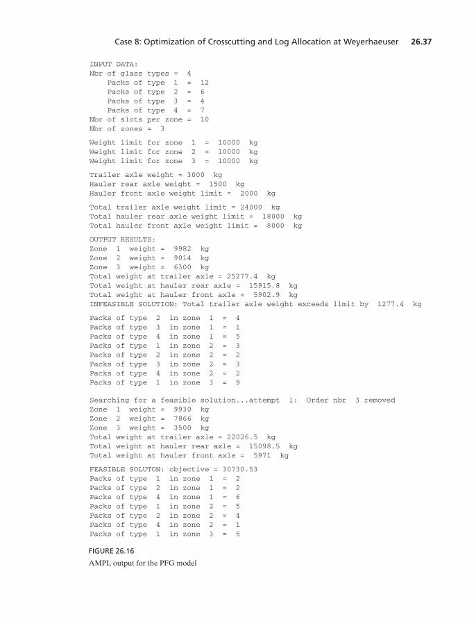
Case 8: Optimization of Crosscutting and Log Allocation at Weyerhaeuser 26.37
INPUT DATA:Nbr of glass types = 4
Packs of type 1 = 12Packs of type 2 = 6Packs of type 3 = 4Packs of type 4 = 7
Nbr of slots per zone = 10Nbr of zones = 3
Weight limit for zone 1 = 10000 kgWeight limit for zone 2 = 10000 kgWeight limit for zone 3 = 10000 kg
Trailer axle weight = 3000 kgHauler rear axle weight = 1500 kgHauler front axle weight limit = 2000 kg
Total trailer axle weight limit = 24000 kgTotal hauler rear axle weight limit = 18000 kgTotal hauler front axle weight limit = 8000 kg
OUTPUT RESULTS:Zone 1 weight = 9982 kgZone 2 weight = 9014 kgZone 3 weight = 6300 kgTotal weight at trailer axle = 25277.4 kgTotal weight at hauler rear axle = 15915.8 kgTotal weight at hauler front axle = 5902.9 kgINFEASIBLE SOLUTION: Total trailer axle weight exceeds limit by 1277.4 kg
Packs of type 2 in zone 1 = 4Packs of type 3 in zone 1 = 1Packs of type 4 in zone 1 = 5Packs of type 1 in zone 2 = 3Packs of type 2 in zone 2 = 2Packs of type 3 in zone 2 = 3Packs of type 4 in zone 2 = 2Packs of type 1 in zone 3 = 9
Searching for a feasible solution...attempt 1: Order nbr 3 removedZone 1 weight = 9930 kgZone 2 weight = 7866 kgZone 3 weight = 3500 kgTotal weight at trailer axle = 22026.5 kgTotal weight at hauler rear axle = 15098.5 kgTotal weight at hauler front axle = 5971 kg
FEASIBLE SOLUTON: objective = 30730.53Packs of type 1 in zone 1 = 2Packs of type 2 in zone 1 = 2Packs of type 4 in zone 1 = 6Packs of type 1 in zone 2 = 5Packs of type 2 in zone 2 = 4Packs of type 4 in zone 2 = 1Packs of type 1 in zone 3 = 5
FIGURE 26.16
AMPL output for the PFG model
M26_TAHA5937_09_SE_C26.QXD 7/26/10 9:27 PM Page 26.37
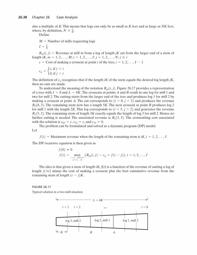
26.38 Chapter 26 Case Analysis
also a multiple of K. This means that logs can only be as small as K feet and as large as NK feet,where, by definition,
Define
of mills requesting logs
at mill m from a log of length jK cut from the larger end of a stem oflength iK,
of making a crosscut at point i of the tree,
The definition of recognizes that if the length iK of the stem equals the desired log length jK,then no cuts are made.
To understand the meaning of the notation Figure 26.17 provides a representationof a tree with and The crosscuts at points A and B result in one log for mill 1 andtwo for mill 2. The cutting starts from the larger end of the tree and produces log 1 for mill 2 bymaking a crosscut at point A. The cut corresponds to and produces the revenue
The remaining stem now has a length 5K. The next crosscut at point B produces log 2for mill 1 with the length 2K. This log corresponds to and generates the revenue
The remaining stem of length 3K exactly equals the length of log 3 for mill 2. Hence nofurther cutting is needed. The associated revenue is The crosscutting cost associatedwith the solution is and
The problem can be formulated and solved as a dynamic program (DP) model.Let
revenue when the length of the remaining stem is iK,
The DP recursive equation is then given as
The idea is that given a stem of length iK, f(i) is a function of the revenue of cutting a log oflength minus the cost of making a crosscut plus the best cumulative revenue from theremaining stem of length 1i - j2K.
j1… i2
f1i2 = maxj = 1,2,Á ,min1i,N2
m = 1,2,Á ,M
5Rm1i, j2 - cij + f1i - j26, i = 1, 2, Á , I
f102 K 0
i = 1, 2, Á , If1i2 = Maximum
c33 = 0.c83 = c, c52 = c,R113, 32.
R115, 22.1i = 5, j = 22
R218, 32.1i = 8, j = 32
L = 8K.I = 8Rm1i, j2,
cij
cij = e c, if j 6 i
0, if j = i
i = 1, 2, Á , I - 1c = Costm = 1, 2, Á , M; i = 1, 2, Á , I; j = 1, 2, Á , N; j … i
Rm1i, j2 = Revenue
I =LK
M = Number
N …LK.
L 8K
K
log 3, mill 2
B A
i 1 i 2 i 8…
log 2, mill 1 log 1, mill 2
FIGURE 26.17
Typical solution in a two-mill situation
M26_TAHA5937_09_SE_C26.QXD 7/26/10 9:27 PM Page 26.38
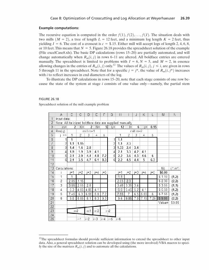
Case 8: Optimization of Crosscutting and Log Allocation at Weyerhaeuser 26.39
12The spreadsheet formulas should provide sufficient information to extend the spreadsheet to other inputdata. Also, a general spreadsheet solution can be developed using (the more involved) VBA macros to speci-fy the size of the matrices and to automate all the calculations.Rm1i, j2
Example computations:
The recursive equation is computed in the order The situation deals withtwo mills a tree of length and a minimum log length thusyielding The cost of a crosscut is Either mill will accept logs of length 2, 4, 6, 8,or 10 feet.This means that Figure 26.18 provides the spreadsheet solution of the example(File excelCase8.xls). The basic DP calculations (rows 15–20) are partially automated, and willchange automatically when in rows 6–11 are altered. All boldface entries are enteredmanually. The spreadsheet is limited to problems with and in essenceallowing changes in the entries of only.12 The values of are given in rows5 through 11 in the spreadsheet. Note that for a specific the value of increaseswith i to reflect increases in end diameters of the log.
To illustrate the DP calculations in rows 15–20, note that each stage consists of one row be-cause the state of the system at stage i consists of one value only—namely, the partial stem
Rm1i, j*2j = j*,Rm1i, j2, j … i,Rm1i, j2
M = 2,I = 6, N = 5,Rm1i, j2
N = 5.c = $.15.I = 6.
K = 2 feet,L = 12 feet,1M = 22,f112, f122, Á , f1I2.
FIGURE 26.18
Spreadsheet solution of the mill example problem
M26_TAHA5937_09_SE_C26.QXD 7/26/10 9:27 PM Page 26.39
26.40 Chapter 26 Case Analysis
length. At stage the (remaining) stem length is 1K, hence resulting in one log only oflength 1K (i.e., ). Also, because no cutting takes place. Thus,
The associated optimum decision at calls for a log of length for mill or
For stage logs can assume a length of 1K or 2K (i.e., or 2) for both mills( or 2). Thus,
The associated optimum decision is which calls for cutting one log of length2K for mill 2.
The remainder of the calculations are carried out in a similar manner as shown in Figure 26.18,rows 15–20. Note that entries B15:F20, H15:L20, and M15:M20 are automated in the spread-sheet. The entries in N15:N20 are created manually after the automated computationsin rows 15–20 are completed. Manually highlighted cells in rows 15–20 define f(i),
The optimum solution is read from cells N15:N20 as follows:
The solution translates to making cuts at and 4 and produces a total value of $9.85 forthe tree.
Practical considerations:
The results of the DP optimization model are used by field operators in the day-to-day operationof the mill. In this regard, the model must be presented in the context of a user-friendly system inwhich the (intimidating) DP calculations are transparent to the user. This is precisely what Lem-berskey and Chi [1] did when they developed the VISION (Video Interactive Stem Inspectionand OptimizatioN) computer system. The system is equipped with a database of large represen-tative samples of tree stems from the regions where trees are harvested. The data include thegeometry of the stem as well as its quality (e.g., location of knots) and the value (in dollars) forstems with different lengths and diameters. In addition, quality characteristics for the differentmills are provided.
A typical user session with VISION includes the following steps:
Step 1. The operator may select a sample stem from the data base or create one using the graph-ic capabilities of VISION. This will result in a realistic representation of the stem on thecomputer screen.The mills requesting the logs are also selected from the data base.
i = 2, 3,
1i = 32: 1j*, m*2 = 11, 12: 1i = 22: 1j*, m*2 = 12, 22 1i = 62: 1j*, m*2 = 12, 22: 1i = 42: 1j*, m*2 = 11, 22:
i = 1, 2, Á , 6.1j*, m*2
1j*, m*2 = 12, 22, = maxE2.05, 1.15, 2.05, 2.3F = 2.3
= max {1.1 - .15 + 1.1, 1.15 - 0 + 0, 1.1 - .15 + 1.1, 2.3 - 0 + 0}
R212, 22 - c22 + f(0)}
f122 = max {R112, 12 - c21 + f112, R112, 22 - c22 + f102, R212, 12 - c21 + f112,m = 1
j = 121i = 22,1j*, m*2 = 11, 22.
21m* = 22,1K1j* = 12i = 1
= 1.1
= max51 - 0 + 0, 1.1 - 0 + 06 f112 = max5R111, 12 - c11 + f102, R211, 12 - c11 + f1026
c11 = 0j = 1i = 1,
M26_TAHA5937_09_SE_C26.QXD 7/26/10 9:27 PM Page 26.40
Case 9: Layout Planning of a Computer Integrated Manufacturing (CIM) Facility 26.41
13Source: C. Benjamin, I. Ehie, and Y. Omurtag, “Planning Facilities at the University of Missouri-Rolla,”Interfaces, Vol. 22, No. 4, pp. 95–105, 1992.
Step 2. After inspecting the stem on the screen, the operator can “cut” the stem into logs basedon experience. Next, an optimum DP solution is requested. In both cases, graphic dis-plays of the created logs together with their associated values are projected on thescreen. The user is then given the chance to compare the two solutions. In particular,the DP solution is examined to make sure that the created logs meet quality specifica-tions. If not, the user may elect to modify the cuts. In each case, the associated value ofthe stem is displayed for comparison.
In VISION, DP optimization is totally transparent to the user. In addition, the interactivegraphic nature of the output makes the system ideal for training operators and improving theirdecision making skills. The design of the system shows how complex mathematical models canbe imbedded within a user-friendly computer system.
Question:
1. Suppose that a third mill that accepts logs of lengths 4, 6, and 8 feet is added to the examplegiven in the case. The new mill has the following R(i, j):
Modify the spreadsheet excelCase8.xls to find the optimum solution for trees of length and
Case 9: Layout Planning for a Computer Integrated Manufacturing (CIM) Facility13
Tools: AHP, GP
Area of application: Facility layout planning
Description of the situation:
In an academic institution a vacated building has been made available to the engineer-ing college to establish a CIM laboratory that will serve as a teaching and research facility as wellas a center of technical excellence for industry. Recommendations are solicited from the facultyregarding a layout plan for the new laboratory. Table 26.11 lists the individual units comprisingthe laboratory together with their ideal and absolute minimum areas. Aisles take at least 15% ofthe total (actual) area. Units 1 through 5 are principally classrooms that must accommodate be-tween 10 and 30 students each.
The ideal areas in Table 26.11 exceed the total area of the vacated building by aboutwhich calls for reducing the areas to be allocated to some of the units.Allocation should
take into account the fact that the new CIM lab has three missions: teaching, research, and serviceto industry. Teaching deals with offering instructions in classroom units 1 through 5. Researchdeals with both consulting contracts and graduate projects, both carried out in the lab. The con-sensus is that the facility will have at least two contracts and six graduate projects at all times.Service to industry comes in the form of continuing education seminars to be conducted in thereception and presentation area (unit 11).
1300 ft2,
5100-ft2
12¿.10¿
R16, 32 = $4.20, R16, 42 = $5.10.R16, 22 = $3.50,R15, 32 = $3.90, R15, 42 = $4.60,R15, 22 = $3.10,R14, 32 = $3.30, R14, 42 = $4.20,R13, 32 = $3.10, R14, 22 = $2.90,
$2.70,R13, 22 =R12, 22 = $2.50,
M26_TAHA5937_09_SE_C26.QXD 7/26/10 9:27 PM Page 26.41
26.42 Chapter 26 Case Analysis
TABLE 26.11 Ideal and Absolute Minimum Unit Areas
Unit Description Ideal area in Absolute Minimum area in
1 Packaging 1450 —2 Production machines 148 —3 Autocad/PC area 120 —4 Physical simulation lab 530 —5 Intelligent control workstations 130 —6 Raw material conversion 165 —7 Assembly 230 1728 Research projects 400 —9 Technician work area 160 120
10 Material storage 360 12611 Reception and presentation area 900 —12 Robot system 140 6013 Automatic storage retrieval system 500 20014 Conveyor systems 200 15015 Aisle space 1000 —
Total 6433
ft2ft2
In support of the three missions of the lab, teaching (T), research (R), and service (S), thecommittee in charge of allocating space has established four principal goals for the facility:
Goal G1: Academic use of the five classrooms is 270 student lab-hours per day, given thatthe daily use of labs 1 through 5 is 5, 5, 4, 4, and 4 hours, respectively . The enrollment in each labis between 10 and 30 students.
Goal G2: Space allocation to the physical simulation lab (unit 4) is as close as possible to theideal area requested
Goal G3: The facility supports a total of 15 simultaneous research contracts and graduateprojects with at least 2 research contracts and 6 research projects being carried out simultane-ously at any one time.
Goal G4: The continuing education facility (unit 11) has a seating capacity of 25 personswith an average of per participant.
Prioritizing the goals:
The situation involves multiple goals, and the first step toward the solution of the problem is toprioritize the goals. AHP (Section 13.1) is an appropriate tool for this purpose. Two sets of com-parison matrices are compiled by each of the five members of the planning committee: The firstset ranks the main areas of teaching, research, and service, and the second set ranks goals G1through G4. Tables 26.12 and 26.13 summarize the rankings provided by the five committeemembers.
The individual comparison matrices for the five members are reduced to a single compari-son matrix using the geometric mean because it guarantees that the elements and of thecombined matrix will satisfy the required reciprocal relationship for alli and j. For example, from Table 26.12, we have
a21 = 25 12 *
13 *
11 *
14 *
13 = .425
a12 = 25 2 * 3 * 1 * 4 * 3 = 2.352
aij =1aji
,ajiaij
20 ft2
1= 530 ft22.
M26_TAHA5937_09_SE_C26.QXD 7/26/10 9:27 PM Page 26.42
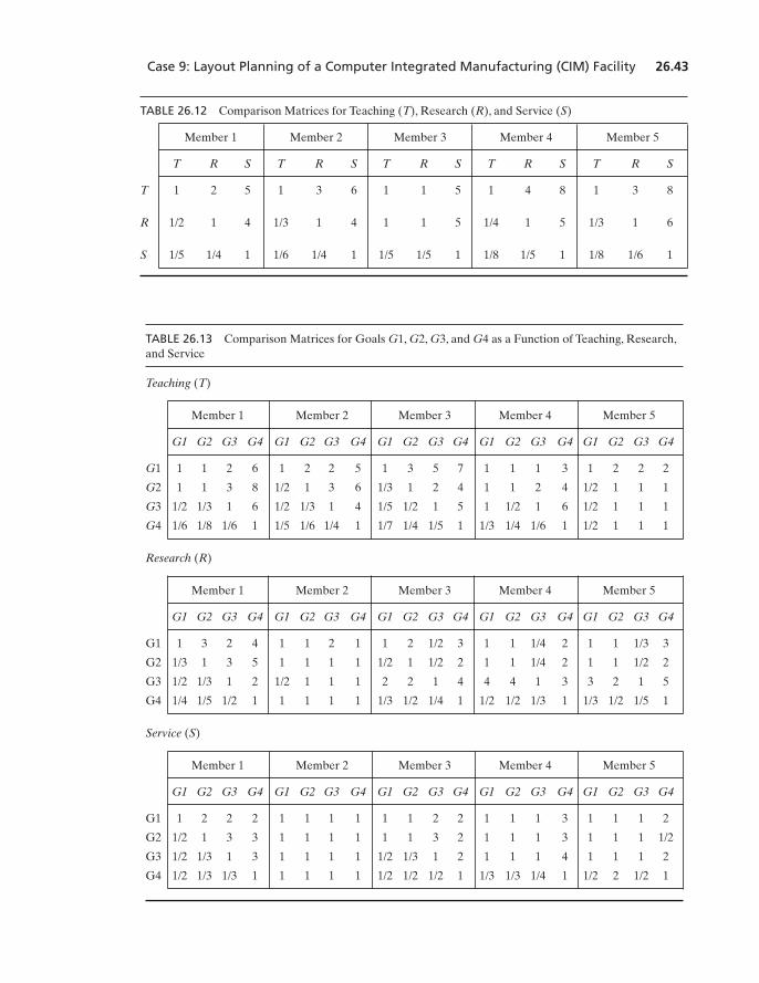
Case 9: Layout Planning of a Computer Integrated Manufacturing (CIM) Facility 26.43
TABLE 26.12 Comparison Matrices for Teaching (T), Research (R), and Service (S)
Member 1 Member 2 Member 3 Member 4 Member 5
T R S T R S T R S T R S T R S
T 1 2 5 1 3 6 1 1 5 1 4 8 1 3 8
R 1/2 1 4 1/3 1 4 1 1 5 1/4 1 5 1/3 1 6
S 1/5 1/4 1 1/6 1/4 1 1/5 1/5 1 1/8 1/5 1 1/8 1/6 1
TABLE 26.13 Comparison Matrices for Goals G1, G2, G3, and G4 as a Function of Teaching, Research,and Service
Teaching (T)
Member 1 Member 2 Member 3 Member 4 Member 5
G1 G2 G3 G4 G1 G2 G3 G4 G1 G2 G3 G4 G1 G2 G3 G4 G1 G2 G3 G4
G1 1 1 2 6 1 2 2 5 1 3 5 7 1 1 1 3 1 2 2 2
G2 1 1 3 8 1/2 1 3 6 1/3 1 2 4 1 1 2 4 1/2 1 1 1
G3 1/2 1/3 1 6 1/2 1/3 1 4 1/5 1/2 1 5 1 1/2 1 6 1/2 1 1 1
G4 1/6 1/8 1/6 1 1/5 1/6 1/4 1 1/7 1/4 1/5 1 1/3 1/4 1/6 1 1/2 1 1 1
Research (R)
Member 1 Member 2 Member 3 Member 4 Member 5
G1 G2 G3 G4 G1 G2 G3 G4 G1 G2 G3 G4 G1 G2 G3 G4 G1 G2 G3 G4
G1 1 3 2 4 1 1 2 1 1 2 1/2 3 1 1 1/4 2 1 1 1/3 3
G2 1/3 1 3 5 1 1 1 1 1/2 1 1/2 2 1 1 1/4 2 1 1 1/2 2
G3 1/2 1/3 1 2 1/2 1 1 1 2 2 1 4 4 4 1 3 3 2 1 5
G4 1/4 1/5 1/2 1 1 1 1 1 1/3 1/2 1/4 1 1/2 1/2 1/3 1 1/3 1/2 1/5 1
Service (S)
Member 1 Member 2 Member 3 Member 4 Member 5
G1 G2 G3 G4 G1 G2 G3 G4 G1 G2 G3 G4 G1 G2 G3 G4 G1 G2 G3 G4
G1 1 2 2 2 1 1 1 1 1 1 2 2 1 1 1 3 1 1 1 2
G2 1/2 1 3 3 1 1 1 1 1 1 3 2 1 1 1 3 1 1 1 1/2
G3 1/2 1/3 1 3 1 1 1 1 1/2 1/3 1 2 1 1 1 4 1 1 1 2
G4 1/2 1/3 1/3 1 1 1 1 1 1/2 1/2 1/2 1 1/3 1/3 1/4 1 1/2 2 1/2 1
M26_TAHA5937_09_SE_C26.QXD 7/26/10 9:27 PM Page 26.43
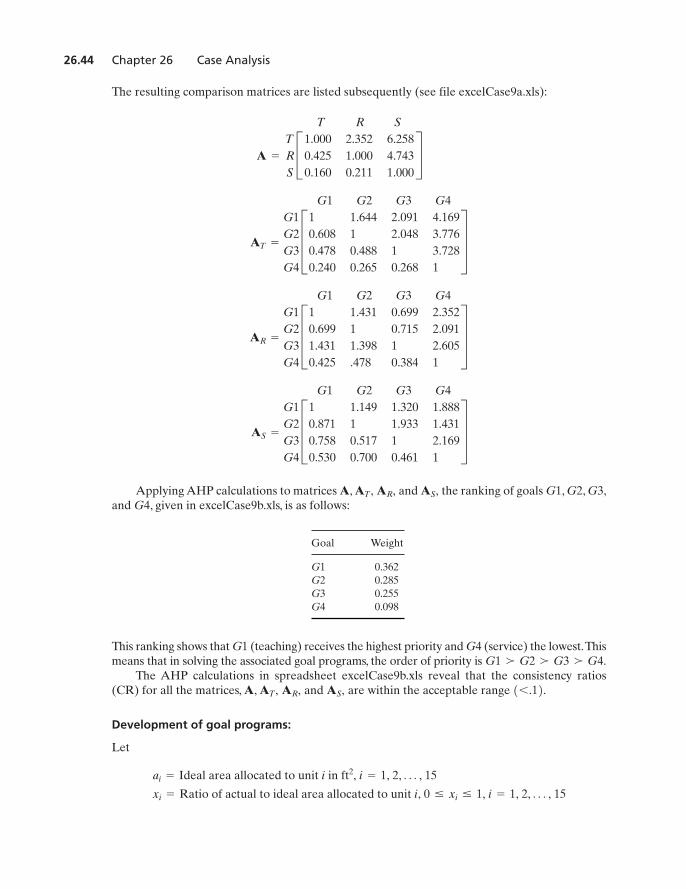
26.44 Chapter 26 Case Analysis
The resulting comparison matrices are listed subsequently (see file excelCase9a.xls):
Applying AHP calculations to matrices A, and the ranking of goals G1, G2, G3,and G4, given in excelCase9b.xls, is as follows:
Goal Weight
G1 0.362G2 0.285G3 0.255G4 0.098
This ranking shows that G1 (teaching) receives the highest priority and G4 (service) the lowest.Thismeans that in solving the associated goal programs, the order of priority is
The AHP calculations in spreadsheet excelCase9b.xls reveal that the consistency ratios(CR) for all the matrices, A, and are within the acceptable range
Development of goal programs:
Let
xi = Ratio of actual to ideal area allocated to unit i, 0 … xi … 1, i = 1, 2, Á , 15
ai = Ideal area allocated to unit i in ft2, i = 1, 2, Á , 15
16 .12.AS,AR,AT,
G1 � G2 � G3 � G4.
AS,AR,AT,
AS =
G1G2G3G4
G1 G2 G3 G4
D1 1.149 1.320 1.8880.871 1 1.933 1.4310.758 0.517 1 2.1690.530 0.700 0.461 1
T
AR =
G1G2G3G4
G1 G2 G3 G4
D1 1.431 0.699 2.3520.699 1 0.715 2.0911.431 1.398 1 2.6050.425 .478 0.384 1
T
AT =
G1G2G3G4
G1 G2 G3 G4
D1 1.644 2.091 4.1690.608 1 2.048 3.7760.478 0.488 1 3.7280.240 0.265 0.268 1
T
A =
T
R
S
T R SC1.000 2.352 6.2580.425 1.000 4.7430.160 0.211 1.000
S
M26_TAHA5937_09_SE_C26.QXD 7/26/10 9:27 PM Page 26.44
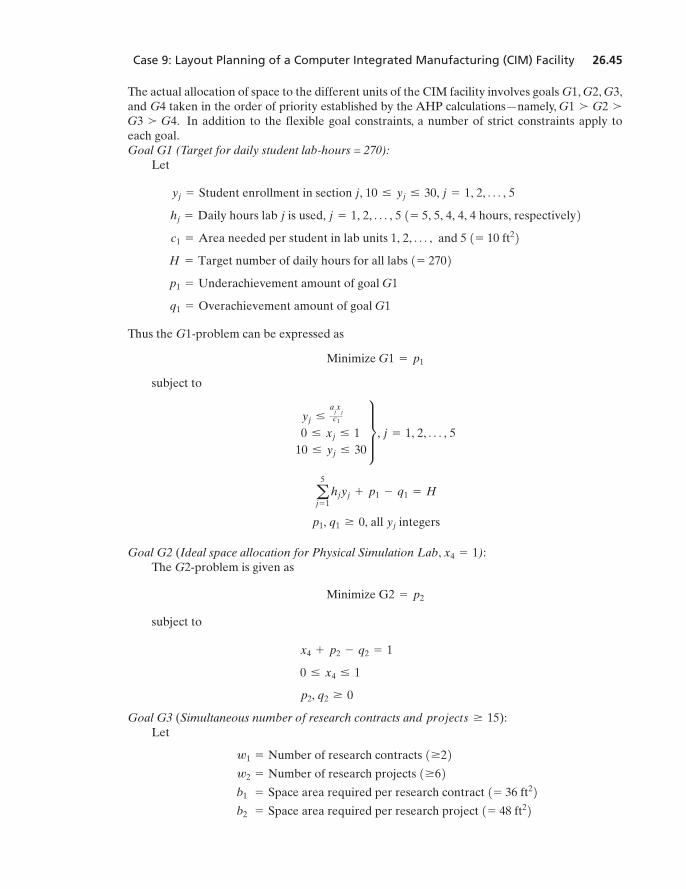
Case 9: Layout Planning of a Computer Integrated Manufacturing (CIM) Facility 26.45
The actual allocation of space to the different units of the CIM facility involves goals G1, G2, G3,and G4 taken in the order of priority established by the AHP calculations—namely,
In addition to the flexible goal constraints, a number of strict constraints apply toeach goal.Goal G1 (Target for daily student lab-hours = 270):
Let
Thus the G1-problem can be expressed as
subject to
Goal G2 (Ideal space allocation for Physical Simulation Lab, ):The G2-problem is given as
subject to
Goal G3 (Simultaneous number of research contracts and ):Let
b2 = Space area required per research project 1= 48 ft22b1 = Space area required per research contract 1= 36 ft22w2 = Number of research projects 1Ú62w1 = Number of research contracts 1Ú22
projects Ú 15
p2, q2 Ú 0
0 … x4 … 1
x4 + p2 - q2 = 1
Minimize G2 = p2
x4 = 1
p1, q1 Ú 0, all yj integers
a5
j = 1hjyj + p1 - q1 = H
yj …
ajx
jc1
0 … xj … 110 … yj … 30
t , j = 1, 2, Á , 5
Minimize G1 = p1
q1 = Overachievement amount of goal G1
p1 = Underachievement amount of goal G1
H = Target number of daily hours for all labs 1= 2702 c1 = Area needed per student in lab units 1, 2, Á , and 5 1= 10 ft22 hj = Daily hours lab j is used, j = 1, 2, Á , 5 1= 5, 5, 4, 4, 4 hours, respectively2 yj = Student enrollment in section j, 10 … yj … 30, j = 1, 2, Á , 5
G3 � G4.G1 � G2 �
M26_TAHA5937_09_SE_C26.QXD 7/26/10 9:27 PM Page 26.45
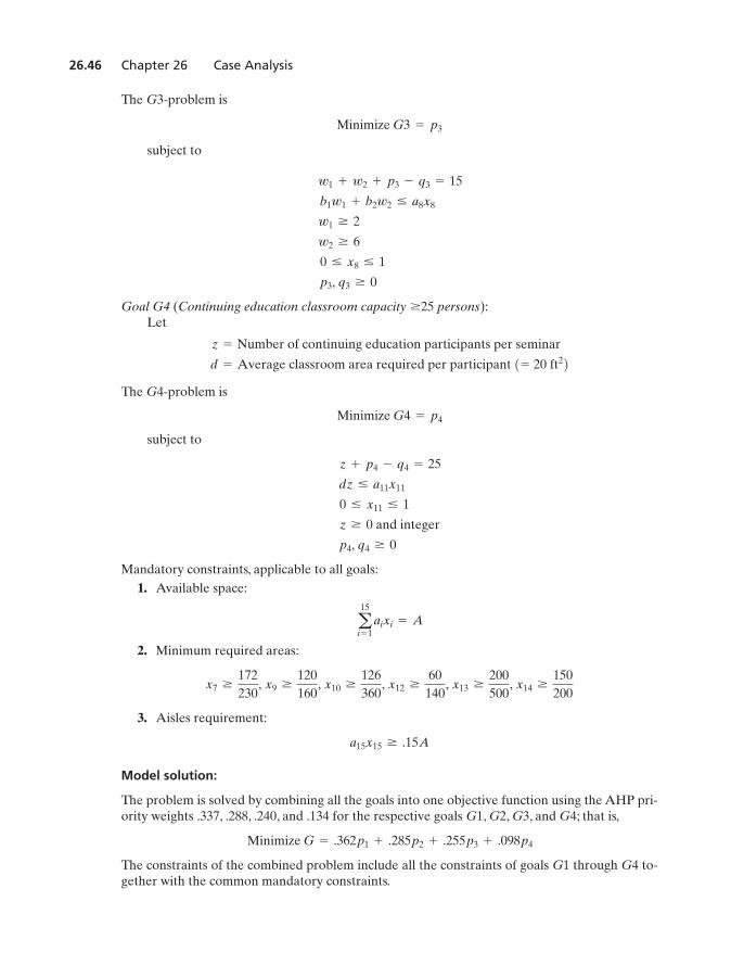
26.46 Chapter 26 Case Analysis
The G3-problem is
subject to
Goal G4 (Continuing education classroom capacity persons):Let
The G4-problem is
subject to
Mandatory constraints, applicable to all goals:1. Available space:
2. Minimum required areas:
3. Aisles requirement:
Model solution:
The problem is solved by combining all the goals into one objective function using the AHP pri-ority weights .337, .288, .240, and .134 for the respective goals G1, G2, G3, and G4; that is,
The constraints of the combined problem include all the constraints of goals G1 through G4 to-gether with the common mandatory constraints.
Minimize G = .362p1 + .285p2 + .255p3 + .098p4
a15x15 Ú .15A
x7 Ú
172230
, x9 Ú
120160
, x10 Ú
126360
, x12 Ú
60140
, x13 Ú
200500
, x14 Ú
150200
a15
i = 1aixi = A
p4, q4 Ú 0
z Ú 0 and integer
0 … x11 … 1
dz … a11x11
z + p4 - q4 = 25
Minimize G4 = p4
d = Average classroom area required per participant 1= 20 ft22 z = Number of continuing education participants per seminar
Ú25
p3, q3 Ú 0
0 … x8 … 1
w2 Ú 6
w1 Ú 2
b1w1 + b2w2 … a8x8
w1 + w2 + p3 - q3 = 15
Minimize G3 = p3
M26_TAHA5937_09_SE_C26.QXD 7/26/10 9:27 PM Page 26.46
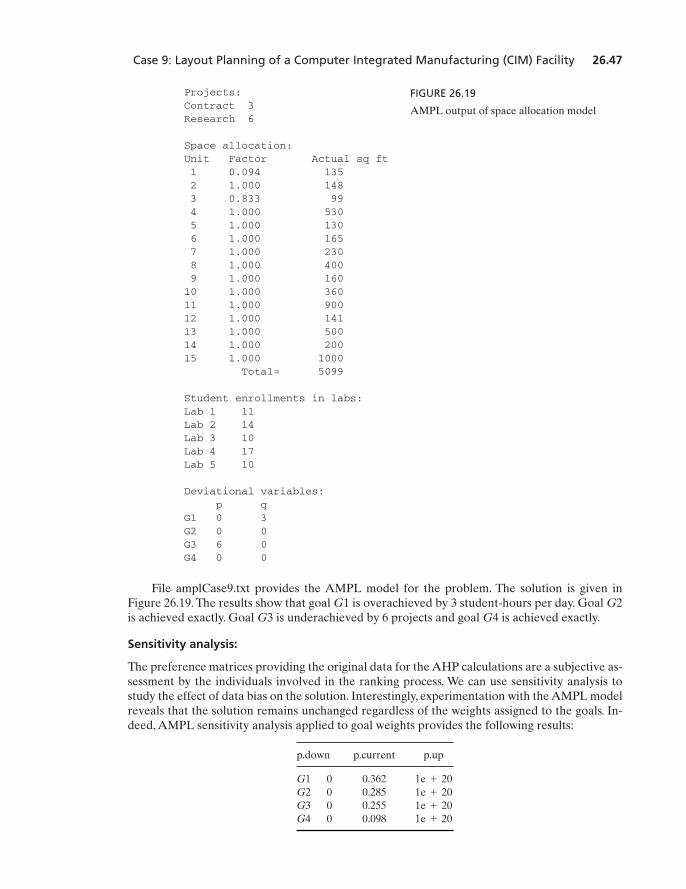
Case 9: Layout Planning of a Computer Integrated Manufacturing (CIM) Facility 26.47
File amplCase9.txt provides the AMPL model for the problem. The solution is given inFigure 26.19. The results show that goal G1 is overachieved by 3 student-hours per day. Goal G2is achieved exactly. Goal G3 is underachieved by 6 projects and goal G4 is achieved exactly.
Sensitivity analysis:
The preference matrices providing the original data for the AHP calculations are a subjective as-sessment by the individuals involved in the ranking process. We can use sensitivity analysis tostudy the effect of data bias on the solution. Interestingly, experimentation with the AMPL modelreveals that the solution remains unchanged regardless of the weights assigned to the goals. In-deed, AMPL sensitivity analysis applied to goal weights provides the following results:
p.down p.current p.up
G1 0 0.362G2 0 0.285G3 0 0.255G4 0 0.098 1e + 20
1e + 201e + 201e + 20
Projects:Contract 3Research 6
Space allocation:Unit Factor Actual sq ft1 0.094 1352 1.000 1483 0.833 994 1.000 5305 1.000 1306 1.000 1657 1.000 2308 1.000 4009 1.000 16010 1.000 36011 1.000 90012 1.000 14113 1.000 50014 1.000 20015 1.000 1000
Total= 5099
Student enrollments in labs:Lab 1 11Lab 2 14Lab 3 10Lab 4 17Lab 5 10
Deviational variables:p q
G1 0 3G2 0 0G3 6 0G4 0 0
FIGURE 26.19
AMPL output of space allocation model
M26_TAHA5937_09_SE_C26.QXD 7/26/10 9:27 PM Page 26.47
26.48 Chapter 26 Case Analysis
14Source: S. Netessine and R. Shumsky, “Introduction to the Theory and Practice of Yield Management,”INFORMS Transactions on Education, Vol. 3, No. 1, pp. 20–28, 2002.
These results show that the optimum solution remains unchanged for any weights between 0 andinfinity. This observation suggests a peculiar feasible solution space, perhaps consisting of a sin-gle point only, and for this reason the optimum solution is independent of the objective function.
The main lesson from the preceding results is that all the AHP calculations carried out earli-er could have been avoided had we formulated the goal programming problem with our best“guesstimates” of the weights for the goals and then studied the impact of changing these weightson the solution. Of course, the manner in which the model has been developed is logical and ourobservation is made only in hindsight. Nevertheless, this experience shows that one should not re-sort to the use of sophisticated analytical tools (such as AHP) before investigating the viability ofusing simpler procedures without impairing the accuracy of the final recommendation.
Question:
1. Suppose that the actual building area is Suppose further that the unit 11 (recep-tion and representation area) ideal request is Find the optimum solution.
Case 10: Booking Limits in Hotel Reservations14
Tool: Decision tree analysis
Area of application: Hotels
Description of the situation:
Hotel La Posada has a total of 300 guest rooms. Its clientele includes both business and leisuretravelers. Rooms can be sold in advance (usually to leisure travelers) at a discount price. Busi-ness travelers, who invariably are late in booking their rooms, pay full price. La Posada must thusestablish a booking limit on the number of discount rooms sold to leisure travelers to take ad-vantage of the full-price business customers.
Mathematical model:
Let N be the number of available rooms and suppose that the current protection level of roomssold at full price is The associated booking limit (rooms sold at a discount)is Figure 26.20 summarizes the situation.
To determine if the protection level should be lowered from to Q, we use the deci-sion tree in Figure 26.21. Let D be the random variable representing historical or forecast de-mand for full-price (business) rooms. Further, let c be the full price and d be the discount price
A decision to lower the protection level from to Q signifies that room willbe sold at the discount price d because there will be ample opportunity to do so. Alternatively,not lowering the protection level will result in two probabilistic outcomes: If the demand forbusiness rooms is greater than or equal to then room will sell at full price, c; elsethe room will not sell at all.The associated probabilities are and re-spectively. It thus follows that the decision to lower the protection level to Q should be adopted if
d Ú cP5D Ú Q + 16 + 0P5D … Q6
P5D … Q6,P5D Ú Q + 16Q + 1Q + 1,
Q + 1Q + 11d 6 c2.
Q + 1N - Q - 1.
Q + 1, 0 … Q 6 N.
1000 ft2.5600 ft2.
M26_TAHA5937_09_SE_C26.QXD 7/26/10 9:27 PM Page 26.48
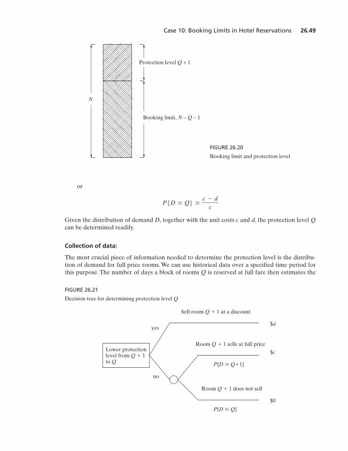
Case 10: Booking Limits in Hotel Reservations 26.49
N
Protection level Q + 1
Booking limit, N – Q – 1
FIGURE 26.20
Booking limit and protection level
Lower protectionlevel from Q 1to Q
Sell room Q 1 at a discount
yes
no
P{D Q 1}
P{D Q}
$d
$c
$0
Room Q 1 sells at full price
Room Q 1 does not sell
FIGURE 26.21
Decision tree for determining protection level Q
or
Given the distribution of demand D, together with the unit costs c and d, the protection level Qcan be determined readily.
Collection of data:
The most crucial piece of information needed to determine the protection level is the distribu-tion of demand for full price rooms. We can use historical data over a specified time period forthis purpose. The number of days a block of rooms Q is reserved at full fare then estimates the
P5D … Q6 Ú
c - dc
M26_TAHA5937_09_SE_C26.QXD 7/26/10 9:27 PM Page 26.49
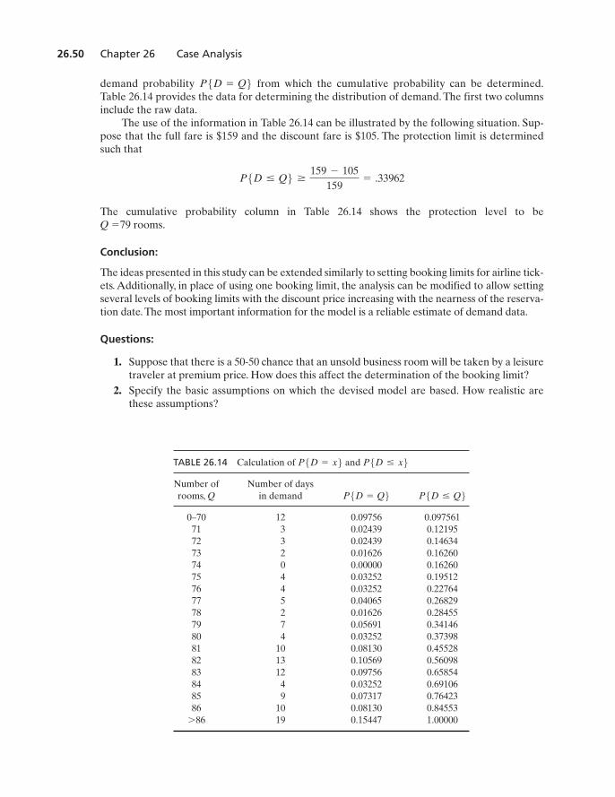
26.50 Chapter 26 Case Analysis
demand probability from which the cumulative probability can be determined.Table 26.14 provides the data for determining the distribution of demand. The first two columnsinclude the raw data.
The use of the information in Table 26.14 can be illustrated by the following situation. Sup-pose that the full fare is $159 and the discount fare is $105. The protection limit is determinedsuch that
The cumulative probability column in Table 26.14 shows the protection level to be
Conclusion:
The ideas presented in this study can be extended similarly to setting booking limits for airline tick-ets. Additionally, in place of using one booking limit, the analysis can be modified to allow settingseveral levels of booking limits with the discount price increasing with the nearness of the reserva-tion date.The most important information for the model is a reliable estimate of demand data.
Questions:
1. Suppose that there is a 50-50 chance that an unsold business room will be taken by a leisuretraveler at premium price. How does this affect the determination of the booking limit?
2. Specify the basic assumptions on which the devised model are based. How realistic arethese assumptions?
79 rooms.Q =
P5D … Q6 Ú
159 - 105159
= .33962
P5D = Q6
TABLE 26.14 Calculation of and
Number of Number of days rooms, Q in demand
0–70 12 0.09756 0.09756171 3 0.02439 0.1219572 3 0.02439 0.1463473 2 0.01626 0.1626074 0 0.00000 0.1626075 4 0.03252 0.1951276 4 0.03252 0.2276477 5 0.04065 0.2682978 2 0.01626 0.2845579 7 0.05691 0.3414680 4 0.03252 0.3739881 10 0.08130 0.4552882 13 0.10569 0.5609883 12 0.09756 0.6585484 4 0.03252 0.6910685 9 0.07317 0.7642386 10 0.08130 0.84553
19 0.15447 1.00000786
P5D … Q6P5D = Q6
P5D … x6P5D = x6
M26_TAHA5937_09_SE_C26.QXD 7/26/10 9:27 PM Page 26.50
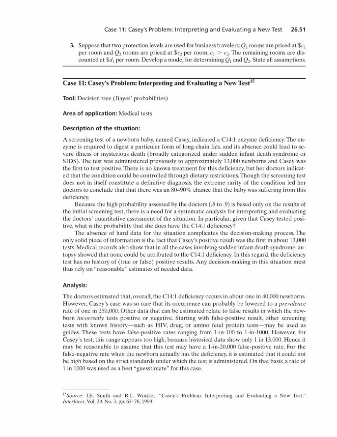
Case 11: Casey’s Problem: Interpreting and Evaluating a New Test 26.51
15Source: J.E. Smith and R.L. Winkler, “Casey’s Problem: Interpreting and Evaluating a New Test,”Interfaces, Vol. 29, No. 3, pp. 63–76, 1999.
3. Suppose that two protection levels are used for business travelers: rooms are priced at per room and rooms are priced at per room, The remaining rooms are dis-counted at per room. Develop a model for determining and State all assumptions.
Case 11: Casey’s Problem: Interpreting and Evaluating a New Test15
Tool: Decision tree (Bayes’ probabilities)
Area of application: Medical tests
Description of the situation:
A screening test of a newborn baby, named Casey, indicated a C14:1 enzyme deficiency. The en-zyme is required to digest a particular form of long-chain fats, and its absence could lead to se-vere illness or mysterious death (broadly categorized under sudden infant death syndrome orSIDS). The test was administered previously to approximately 13,000 newborns and Casey wasthe first to test positive. There is no known treatment for this deficiency, but her doctors indicat-ed that the condition could be controlled through dietary restrictions.Though the screening testdoes not in itself constitute a definitive diagnosis, the extreme rarity of the condition led herdoctors to conclude that that there was an 80–90% chance that the baby was suffering from thisdeficiency.
Because the high probability assessed by the doctors (.8 to .9) is based only on the results ofthe initial screening test, there is a need for a systematic analysis for interpreting and evaluatingthe doctors’ quantitative assessment of the situation. In particular, given that Casey tested posi-tive, what is the probability that she does have the C14:1 deficiency?
The absence of hard data for the situation complicates the decision-making process. Theonly solid piece of information is the fact that Casey’s positive result was the first in about 13,000tests. Medical records also show that in all the cases involving sudden infant death syndrome, au-topsy showed that none could be attributed to the C14:1 deficiency. In this regard, the deficiencytest has no history of (true or false) positive results. Any decision-making in this situation mustthus rely on “reasonable” estimates of needed data.
Analysis:
The doctors estimated that, overall, the C14:1 deficiency occurs in about one in 40,000 newborns.However, Casey’s case was so rare that its occurrence can probably be lowered to a prevalencerate of one in 250,000. Other data that can be estimated relate to false results in which the new-born incorrectly tests positive or negative. Starting with false-positive result, other screeningtests with known history—such as HIV, drug, or amino fetal protein tests—may be used asguides. These tests have false-positive rates ranging from 1-in-100 to 1-in-1000. However, forCasey’s test, this range appears too high, because historical data show only 1 in 13,000. Hence itmay be reasonable to assume that this test may have a 1-in-20,000 false-positive rate. For thefalse-negative rate when the newborn actually has the deficiency, it is estimated that it could notbe high based on the strict standards under which the test is administered. On that basis, a rate of1 in 1000 was used as a best “guesstimate” for this case.
Q2.Q1$d1
c1 7 c2.$c2Q2
$c1Q1
M26_TAHA5937_09_SE_C26.QXD 7/26/10 9:27 PM Page 26.51
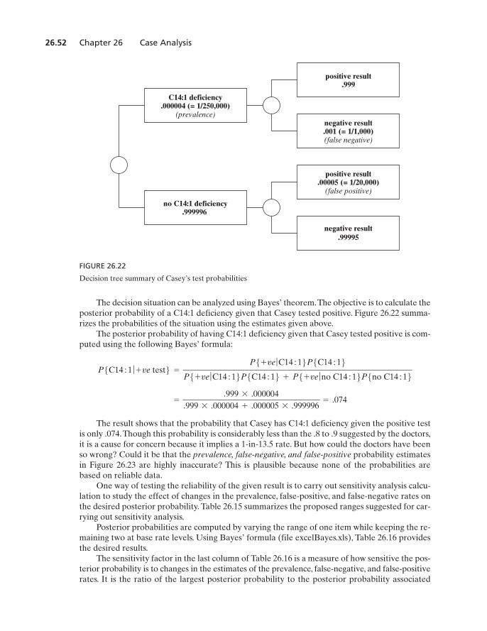
26.52 Chapter 26 Case Analysis
The decision situation can be analyzed using Bayes’ theorem.The objective is to calculate theposterior probability of a C14:1 deficiency given that Casey tested positive. Figure 26.22 summa-rizes the probabilities of the situation using the estimates given above.
The posterior probability of having C14:1 deficiency given that Casey tested positive is com-puted using the following Bayes’ formula:
The result shows that the probability that Casey has C14:1 deficiency given the positive testis only .074.Though this probability is considerably less than the .8 to .9 suggested by the doctors,it is a cause for concern because it implies a 1-in-13.5 rate. But how could the doctors have beenso wrong? Could it be that the prevalence, false-negative, and false-positive probability estimatesin Figure 26.23 are highly inaccurate? This is plausible because none of the probabilities arebased on reliable data.
One way of testing the reliability of the given result is to carry out sensitivity analysis calcu-lation to study the effect of changes in the prevalence, false-positive, and false-negative rates onthe desired posterior probability. Table 26.15 summarizes the proposed ranges suggested for car-rying out sensitivity analysis.
Posterior probabilities are computed by varying the range of one item while keeping the re-maining two at base rate levels. Using Bayes’ formula (file excelBayes.xls), Table 26.16 providesthe desired results.
The sensitivity factor in the last column of Table 26.16 is a measure of how sensitive the pos-terior probability is to changes in the estimates of the prevalence, false-negative, and false-positiverates. It is the ratio of the largest posterior probability to the posterior probability associated
=
.999 * .000004.999 * .000004 + .000005 * .999996
= .074
P5C14 : 1 ƒ +ve test6 =
P5+ve ƒ C14 : 16P5C14 : 16P5+ve ƒ C14 : 16P5C14 : 16 + P5+ve ƒ no C14 : 16P5no C14 : 16
C14:1 deficiency.000004 (= 1/250,000)
(prevalence)
positive result.999
negative result.001 (= 1/1,000)(false negative)
no C14:1 deficiency.999996
positive result.00005 (= 1/20,000)
(false positive)
negative result.99995
FIGURE 26.22
Decision tree summary of Casey’s test probabilities
M26_TAHA5937_09_SE_C26.QXD 7/26/10 9:27 PM Page 26.52
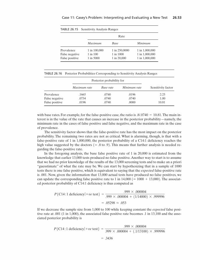
Case 11: Casey’s Problem: Interpreting and Evaluating a New Test 26.53
TABLE 26.16 Posterior Probabilities Corresponding to Sensitivity Analysis Ranges
Posterior probability for
Maximum rate Base rate Minimum rate Sensitivity factor
Prevalence .1665 .0740 .0196 2.25False negative .0734 .0740 .0740 1.00False positive .0196 .0740 .8000 10.81
with base rates. For example, for the false-positive case, the ratio is The main in-terest is in the value of the rate that causes an increase in the posterior probability—namely, theminimum rate in the cases of false positive and false negative, and the maximum rate in the caseof prevalence.
The sensitivity factor shows that the false-positive rate has the most impact on the posteriorprobability. The remaining two rates are not as critical. What is alarming, though, is that with afalse-positive rate of 1 in 1,000,000, the posterior probability of a C14:1 deficiency reaches thehigh value suggested by the doctors This means that further analysis is needed re-garding the false-positive rate.
In the foregoing analysis, the base false positive rate of 1 in 20,000 is estimated from theknowledge that earlier 13,000 tests produced no false positive. Another way to start is to assumethat we had no prior knowledge of the results of the 13,000 screening tests and to make an a priori“guesstimate” of what the rate may be. We can start by hypothesizing that in a sample of 1000tests there is one false positive, which is equivalent to saying that the expected false-positive rateis .001. Now, given the information that 13,000 actual tests have produced no false positives, wecan update the corresponding false positive rate to 1 in The associat-ed posterior probability of C14:1 deficiency is thus computed as
If we decrease the sample size from 1,000 to 100 while keeping constant the expected false posi-tive rate at .001 (1 in 1,000), the associated false positive rate becomes .1 in 13,100 and the asso-ciated posterior probability is
= .3436
P5C14 : 1 deficiency ƒ +ve test6 =
.999 * .000004.999 * .000004 + 1.1/131002 * .999996
= .05298 L .053
P5C14 : 1 deficiency ƒ +ve test6 =
.999 * .000004.999 * .000004 + 11/140002 * .999996
14,000 1= 1000 + 13,0002.
1= .8 to .92.
.8/.0740 = 10.81.
TABLE 26.15 Sensitivity Analysis Ranges
Rate
Maximum Base Minimum
Prevalence 1 in 100,000 1 in 250,0000 1 in 1,000,000False negative 1 in 100 1 in 1000 1 in 1,000,000False positive 1 in 5000 1 in 20,000 1 in 1,000,000
M26_TAHA5937_09_SE_C26.QXD 7/26/10 9:27 PM Page 26.53
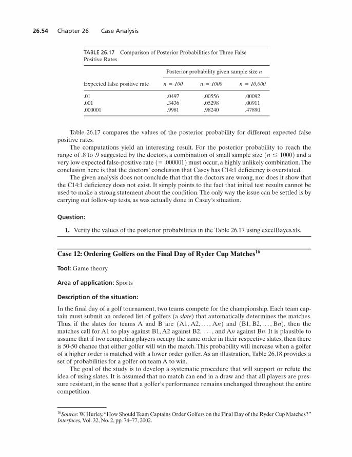
26.54 Chapter 26 Case Analysis
Table 26.17 compares the values of the posterior probability for different expected falsepositive rates.
The computations yield an interesting result. For the posterior probability to reach therange of .8 to .9 suggested by the doctors, a combination of small sample size and avery low expected false-positive rate must occur, a highly unlikely combination.Theconclusion here is that the doctors’ conclusion that Casey has C14:1 deficiency is overstated.
The given analysis does not conclude that that the doctors are wrong, nor does it show thatthe C14:1 deficiency does not exist. It simply points to the fact that initial test results cannot beused to make a strong statement about the condition. The only way the issue can be settled is bycarrying out follow-up tests, as was actually done in Casey’s situation.
Question:
1. Verify the values of the posterior probabilities in the Table 26.17 using excelBayes.xls.
Case 12: Ordering Golfers on the Final Day of Ryder Cup Matches16
Tool: Game theory
Area of application: Sports
Description of the situation:
In the final day of a golf tournament, two teams compete for the championship. Each team cap-tain must submit an ordered list of golfers (a slate) that automatically determines the matches.Thus, if the slates for teams A and B are and then thematches call for A1 to play against B1, A2 against B2, and An against Bn. It is plausible toassume that if two competing players occupy the same order in their respective slates, then thereis 50-50 chance that either golfer will win the match. This probability will increase when a golferof a higher order is matched with a lower order golfer. As an illustration, Table 26.18 provides aset of probabilities for a golfer on team A to win.
The goal of the study is to develop a systematic procedure that will support or refute theidea of using slates. It is assumed that no match can end in a draw and that all players are pres-sure resistant, in the sense that a golfer’s performance remains unchanged throughout the entirecompetition.
Á ,1B1, B2, Á , Bn2,1A1, A2, Á , An2
1= .00000121n … 10002
TABLE 26.17 Comparison of Posterior Probabilities for Three False Positive Rates
Posterior probability given sample size n
Expected false positive rate
.01 .0497 .00556 .00092
.001 .3436 .05298 .00911
.000001 .9981 .98240 .47890
n = 10,000n = 1000n = 100
16Source: W. Hurley,“How Should Team Captains Order Golfers on the Final Day of the Ryder Cup Matches?”Interfaces, Vol. 32, No. 2, pp. 74–77, 2002.
M26_TAHA5937_09_SE_C26.QXD 7/26/10 9:27 PM Page 26.54
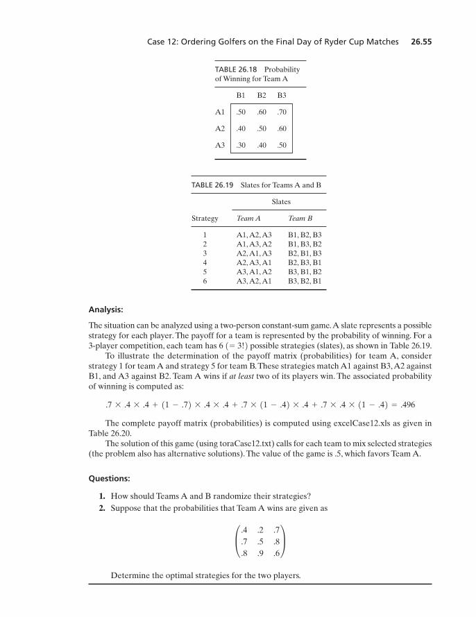
Case 12: Ordering Golfers on the Final Day of Ryder Cup Matches 26.55
TABLE 26.19 Slates for Teams A and B
Slates
Strategy Team A Team B
1 A1, A2, A3 B1, B2, B32 A1, A3, A2 B1, B3, B23 A2, A1, A3 B2, B1, B34 A2, A3, A1 B2, B3, B15 A3, A1, A2 B3, B1, B26 A3, A2, A1 B3, B2, B1
Analysis:
The situation can be analyzed using a two-person constant-sum game.A slate represents a possiblestrategy for each player. The payoff for a team is represented by the probability of winning. For a3-player competition, each team has possible strategies (slates), as shown in Table 26.19.
To illustrate the determination of the payoff matrix (probabilities) for team A, considerstrategy 1 for team A and strategy 5 for team B.These strategies match A1 against B3,A2 againstB1, and A3 against B2. Team A wins if at least two of its players win. The associated probabilityof winning is computed as:
The complete payoff matrix (probabilities) is computed using excelCase12.xls as given inTable 26.20.
The solution of this game (using toraCase12.txt) calls for each team to mix selected strategies(the problem also has alternative solutions). The value of the game is .5, which favors Team A.
Questions:
1. How should Teams A and B randomize their strategies?2. Suppose that the probabilities that Team A wins are given as
Determine the optimal strategies for the two players.
£ .4 .2 .7.7 .5 .8.8 .9 .6
≥
.7 * .4 * .4 + 11 - .72 * .4 * .4 + .7 * 11 - .42 * .4 + .7 * .4 * 11 - .42 = .496
6 1= 3!2
TABLE 26.18 Probability of Winning for Team A
B1 B2 B3
A1 .50 .60 .70
A2 .40 .50 .60
A3 .30 .40 .50
M26_TAHA5937_09_SE_C26.QXD 7/26/10 9:27 PM Page 26.55
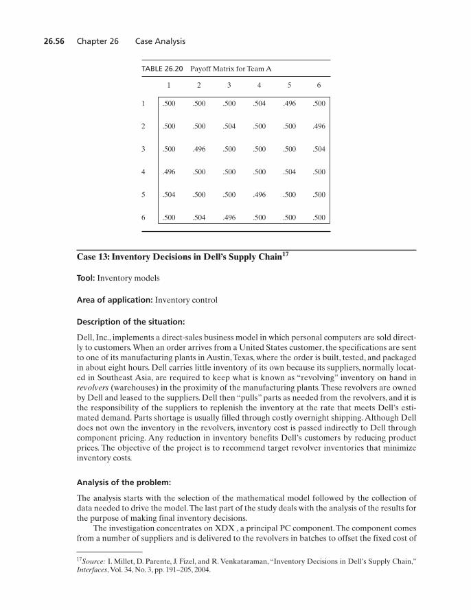
26.56 Chapter 26 Case Analysis
TABLE 26.20 Payoff Matrix for Team A
1 2 3 4 5 6
1 .500 .500 .500 .504 .496 .500
2 .500 .500 .504 .500 .500 .496
3 .500 .496 .500 .500 .500 .504
4 .496 .500 .500 .500 .504 .500
5 .504 .500 .500 .496 .500 .500
6 .500 .504 .496 .500 .500 .500
Case 13: Inventory Decisions in Dell’s Supply Chain17
Tool: Inventory models
Area of application: Inventory control
Description of the situation:
Dell, Inc., implements a direct-sales business model in which personal computers are sold direct-ly to customers.When an order arrives from a United States customer, the specifications are sentto one of its manufacturing plants in Austin, Texas, where the order is built, tested, and packagedin about eight hours. Dell carries little inventory of its own because its suppliers, normally locat-ed in Southeast Asia, are required to keep what is known as “revolving” inventory on hand inrevolvers (warehouses) in the proximity of the manufacturing plants. These revolvers are ownedby Dell and leased to the suppliers. Dell then “pulls” parts as needed from the revolvers, and it isthe responsibility of the suppliers to replenish the inventory at the rate that meets Dell’s esti-mated demand. Parts shortage is usually filled through costly overnight shipping. Although Delldoes not own the inventory in the revolvers, inventory cost is passed indirectly to Dell throughcomponent pricing. Any reduction in inventory benefits Dell’s customers by reducing productprices. The objective of the project is to recommend target revolver inventories that minimizeinventory costs.
Analysis of the problem:
The analysis starts with the selection of the mathematical model followed by the collection ofdata needed to drive the model.The last part of the study deals with the analysis of the results forthe purpose of making final inventory decisions.
The investigation concentrates on XDX , a principal PC component. The component comesfrom a number of suppliers and is delivered to the revolvers in batches to offset the fixed cost of
17Source: I. Millet, D. Parente, J. Fizel, and R. Venkataraman, “Inventory Decisions in Dell’s Supply Chain,”Interfaces, Vol. 34, No. 3, pp. 191–205, 2004.
M26_TAHA5937_09_SE_C26.QXD 7/26/10 9:27 PM Page 26.56
Case 13: Inventory Decisions in Dell’s Supply Chain 26.57
18G. Hadley and T. Whitin, Analysis of Inventory Systems, Prentice Hall, Englewood Cliffs, NJ, 1963, p. 153.
ordering. The inventory policy followed by each supplier is to deliver a new batch whenever theinventory level drops to a certain level. However, it has been noticed that both the batch size andthe reorder level are considerably inconsistent among the suppliers. The first task then was tobring consistency to the suppliers’ ordering policies. The model selected to represent the situa-tion is the (Q, R) policy, where Q is the batch size and R is the reorder level. Historical data re-veal that the order quantity Q is constant and the inconsistency in the ordering policy stems fromthe wide variation in the reorder level and the lead time between placing an order and receivingit. Consequently, a decision is made to maintain Q at its current level and to concentrate on thedetermination of R.
It is reasonable to assume that the demand x during lead time is normal with mean andstandard deviation The standard normal distribution of the lead time demand is thus de-fined as
Next, let be the probability of running out of stock during lead time that Dell is willing to tol-erate, and define Z such that then the reorder level R is
We can use an approximation borrowed from the single-period newsvendor inventory modelto determine Z heuristically (see Section 14.2). The single-period model can be justified by thefact that the component XDX has limited shelf life because of obsolescence. Given that p is thepenalty cost per unit of unsatisfied demand and h is the holding cost per unit of surplus inventory,we have
The function is the CDF of the standard normal distribution. Thus,
The mean and standard deviation of the demand during lead time are a function of tworandom variables: lead time and the demand per unit time. Under certain assumptions of inde-pendence, it can be proved that18
where
st = Standard deviation of the lead time
sd = Standard deviation of the demand
T = Average lead time in time units
D = Average demand in units per unit time
s = 2D2st2
+ Tsd2
m = DT
sm
Z = £-1a p
p + hb
£1Z2£1Z2 K P5z … Z6 =
p
p + h
R = m + Zs
P5z … Z] = 1 - a;a
z =
x - m
s
s.m
M26_TAHA5937_09_SE_C26.QXD 7/26/10 9:27 PM Page 26.57
26.58 Chapter 26 Case Analysis
Based on this model and given that the order quantity is fixed at Q units, the inventory policy is“order Q units of XDX whenever the inventory level in the revolvers drops to R units.”
Data collection:
Data collection originates from three suppliers, A, B, and C, who replenish Dell’s revolvers withdifferent but totally interchangeable XDX parts. The data for the model were collected for theperiod from December 1, 1998, to May 27, 1999, in two groups: (1) those related to the estimationof the holding and penalty costs, p and h, and (2) those used to estimate the mean and varianceof demand during lead time.
The estimation of the holding cost, h, is based on the time period between two consecutivedeliveries and includes the cost of capital tied up in the revolvers, price erosion due to obsoles-cence, and the storage charge assessed by Dell.The penalty cost, p, is estimated based on two fac-tors: lost profit from canceled or partially filled orders and increased shipping cost when the partis not available when needed.
The demand during lead time is estimated based on a number of factors: (1) Dell’s dailyconsumption (called pulls) from the revolvers, (2) daily receipts from the suppliers at the re-volvers, (3) daily in-transit inventory from the suppliers to the revolvers, (4) daily PC sales usingXDX components, (5) Dell’s forecasts to suppliers regarding the expected use of XDX duringnext month, and (6) suppliers’ lead times.
Data analysis:
The first task in the data analysis is to assess whether or not the inventory policies of the threesuppliers of XDX have been operating optimally according to the proposed (R, Q) policy. Thishypothesis is tested by computing the Z-score for all placed orders during the data collection pe-riod (December 1, 1998, to May 27, 1999). Specifically, given the actual reorder level R and theestimated mean and variance of the demand (per day) and the lead time (in days), the formulaspresented above yield
The computations reveal that Z varies significantly from .8 to 5.2 over the study period. Giventhat the estimated holding and penalty costs, h and p, are the same for all three suppliers, theZ-score under optimal conditions should remain steady at about The fact thatthe ordering policy of the suppliers exhibits such erratic variations (between .8 and 5.2) indicatesthat they are not operating under optimal inventory policy. This discrepancy led the study teamto investigate the reasons behind the current practice.
A supplier bases its replenishment policy on the monthly forecasts provided by Dell. Theseforecasts can occur at three levels: (1) aggregate representing the total number of PCs over thenext month, (2) attach representing the number of PC units that will be using the componentXDX, and (3) pull representing the number of XDX units that Dell will be withdrawing from therevolvers of each supplier. The effect of errors in aggregate, attach, and pull forecasts is a corre-sponding increase in the variability in demand, expressed in terms of the variance of the distrib-ution of demand. An investigation of the three types of forecast revealed that Dell’s forecasterrors are responsible for approximately 50% of the total inventory carried in the revolvers,mainly because the suppliers are trying to compensate for the large variance by maintaining alarger safety stock. This information is important because, aside from the implementation of theoptimal (R, Q) system based on the present “inconsistent” forecasts, Dell can play an importantrole in reducing the inventory in the revolvers by instituting more stringent forecasting techniques.
Z = £-1 A p
p + h B .
Z =
R - DT
2D2st2
+ Tsd2
M26_TAHA5937_09_SE_C26.QXD 7/26/10 9:27 PM Page 26.58
Case 14: Analysis of an Internal Transport System in a Manufacturing Plant 26.59
19Source: G. P. Cosmetatos,“The Value of Queuing Theory—A Case Study,” Interfaces,Vol. 9, No. 3, pp. 47–51,1979.
In particular, the pull forecast error is attributed primarily to the fact that Dell withdraws need-ed XDX units from one supplier at a time instead of in fixed ratios from all suppliers. The effectof “clump” pulling of XDX from the revolvers gives rise to higher replenishment rates and hencelarger safety stocks.
Conclusions:
The results of the investigation indicate that eliminating clump pulling and providing more reli-able forecasts can potentially reduce the safety stock by as much as 38%. So far, Dell has decreasedinventories for one of its lines by about 20% with estimated annual savings of $2.7 million. Perhapsthe most remarkable observation about the study is recognizing that the inventory level can bereduced by eliminating the source of variation due to forecast errors.This result is confirmed bythe fact that the optimal reorder level depends directly on the standard deviation of demand.
Questions:
1. Evaluate the adverse effect of “clump” pulling from revolvers by comparing its averagelevel of inventory with that when pulling is made uniformly from all the suppliers.
2. Suppose that the average demand per day in one assembly line is N(300, 10) and the de-mand during lead time is N(50,4). Given that the penalty cost per unit of unsatisfieddemand per day is $100 and the holding cost per surplus inventory unit per day is $5, de-termine the reorder level.
3. For the data in Question 2, study the sensitivity of the reorder level to a error in theestimation of the average demand per day (r varies from 0 to 50). The standard deviationremains unchanged.
Case 14: Analysis of an Internal Transport System in a Manufacturing Plant19
Tools: Queuing theory, simulation
Area of application: Materials handling
Description of the situation:
Three trucks are used to transport materials within in a manufacturing plant. The trucks wait ina central parking lot until requested.A requested truck will travel to the customer location, carryload to destination, and then return to the central parking lot. The principal user of the service isproduction (P) followed by the workshop (W) and maintenance (M). Other departments (O)occasionally may request the use of the trucks. Complaints about the long wait for a free truckhave prompted users, especially production, to request adding a fourth truck to the fleet. Thestudy is concerned with the justification of the cost for a fourth truck.
Input data summary:
Information on the operation of the internal transport system was collected over a period of 17consecutive two-shift work days. Tables 26.21 and 26.22 provide a summary of the collected data.
;r%
M26_TAHA5937_09_SE_C26.QXD 7/26/10 9:27 PM Page 26.59
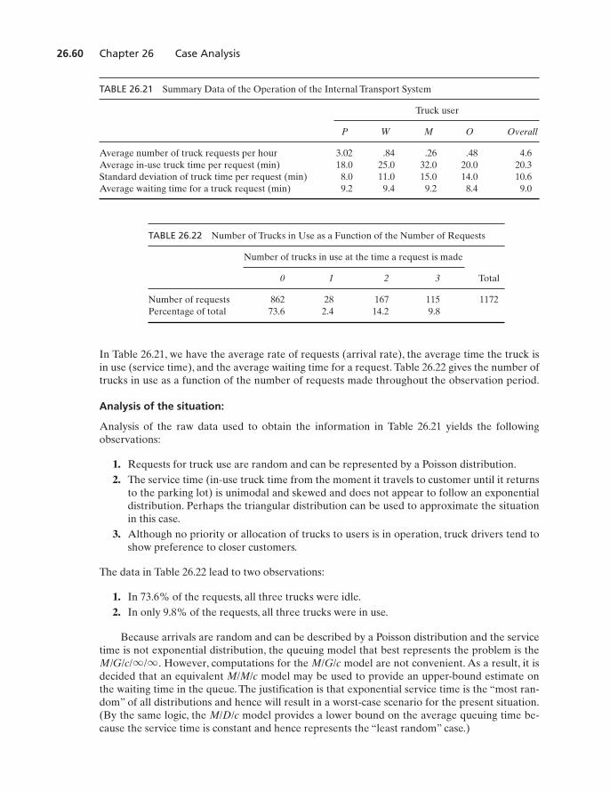
26.60 Chapter 26 Case Analysis
In Table 26.21, we have the average rate of requests (arrival rate), the average time the truck isin use (service time), and the average waiting time for a request. Table 26.22 gives the number oftrucks in use as a function of the number of requests made throughout the observation period.
Analysis of the situation:
Analysis of the raw data used to obtain the information in Table 26.21 yields the followingobservations:
1. Requests for truck use are random and can be represented by a Poisson distribution.2. The service time (in-use truck time from the moment it travels to customer until it returns
to the parking lot) is unimodal and skewed and does not appear to follow an exponentialdistribution. Perhaps the triangular distribution can be used to approximate the situationin this case.
3. Although no priority or allocation of trucks to users is in operation, truck drivers tend toshow preference to closer customers.
The data in Table 26.22 lead to two observations:
1. In 73.6% of the requests, all three trucks were idle.2. In only 9.8% of the requests, all three trucks were in use.
Because arrivals are random and can be described by a Poisson distribution and the servicetime is not exponential distribution, the queuing model that best represents the problem is the
However, computations for the M/G/c model are not convenient. As a result, it isdecided that an equivalent M/M/c model may be used to provide an upper-bound estimate onthe waiting time in the queue. The justification is that exponential service time is the “most ran-dom” of all distributions and hence will result in a worst-case scenario for the present situation.(By the same logic, the M/D/c model provides a lower bound on the average queuing time be-cause the service time is constant and hence represents the “least random” case.)
M/G/c/q /q .
TABLE 26.21 Summary Data of the Operation of the Internal Transport System
Truck user
P W M O Overall
Average number of truck requests per hour 3.02 .84 .26 .48 4.6Average in-use truck time per request (min) 18.0 25.0 32.0 20.0 20.3Standard deviation of truck time per request (min) 8.0 11.0 15.0 14.0 10.6Average waiting time for a truck request (min) 9.2 9.4 9.2 8.4 9.0
TABLE 26.22 Number of Trucks in Use as a Function of the Number of Requests
Number of trucks in use at the time a request is made
0 1 2 3 Total
Number of requests 862 28 167 115 1172Percentage of total 73.6 2.4 14.2 9.8
M26_TAHA5937_09_SE_C26.QXD 7/26/10 9:27 PM Page 26.60
Case 14: Analysis of an Internal Transport System in a Manufacturing Plant 26.61
The following is a summary of the results of the M/M/c model for re-quest per minute and service per minute:
Probability that the system is empty,
Probability of at least three requests in the system,
Average length of queue, request
Average waiting time in queue, minutes
Looking at these results, one notices makes the perplexing observation that the upperbound on the average waiting time in the queue (estimated from the M/M/c model) is muchlower than what is actually observed ( minutes versus the observed 9.0 minutes given inTable 26.21). This observation leads to one of two conclusions: Either the estimates of and are highly inaccurate or the estimate of the average waiting is unreliable. A careful study ofthe data shows that the data are indeed reliable. To reinforce the results of the M/M/c model,simulation is used in which the service time distribution is approximated by a triangular dis-tribution with parameters (15, 20.3, 30). The middle value represents the observed averageservice time and the lower and upper values are estimated based on the standard deviation ofservice time and the observed minimum and maximum service times. Thesimulation can be carried out using Excel template excelMultiServer.xls with Poisson arrivalrate of .0767 request per minute and triangular service time. With 10 replications that simu-late 450 requests each, the average queuing time was found to vary from a minimum of 1.1minutes to a maximum of 3.62 minutes and an average value of 2.07 minutes. This result gavemore credence to the upper bound result of 3.6 minutes obtained from the M/M/c model.Moreover, the high waiting time obtained from the observed data seems tocontradict the data in Table 26.22, where 73.6% of the time all three trucks were idle when aservice request arrived.
How can this inconsistency between observed and estimated results be resolved? Goingback to the plant floor to further study the operation of the transport system, an analyst madea fortunate observation: The layout of the parking lot was such that waiting trucks could notbe seen by the users, who then assumed that no trucks were available. This in essence wasequivalent to operating with less than three trucks, which in turn resulted in an artificial in-crease in waiting time. Once this problem had been discovered, the solution became obvious:Provide the truck drivers and the users with a two-way communication system. The proposedsolution led to immediate improvement in service and a noticeable decrease in the waitingtime.
Although the proposed solution was not “propelled” by queuing results in a direct manner,it was the logic inherent in queuing analysis that led to the discovery of data inconsistency and,hence, to pinpointing the source of the problem.
Questions:
1. In Table 26.21, how are the values in the “overall” column computed?2. If 95% of the requests for a truck come from production and only 5% come from the re-
maining departments, how would you analyze the situation?3. Evaluate the robustness of the results by studying the sensitivity of simulation results to
changes in the minimum and maximum values of the triangular distribution. Does the sen-sitivity analysis confirm or refute the conclusion given for the case?
1= 9.0 minutes2
1= 10.6 minutes2
ml
Wq = 3.6
Wq = 3.6
Lq = .277
pn Ú 3 = .133
p0 = .197
m =1
20.3 = .0493l =
4.660 = .0767c = 3,
M26_TAHA5937_09_SE_C26.QXD 7/26/10 9:27 PM Page 26.61
26.62 Chapter 26 Case Analysis
Case 15: Telephone Sales Manpower Planning at Qantas Airways20
Tools: ILP, queuing theory
Area of application: Airlines
Description of the situation:
To reduce operating costs, Qantas Airways seeks to staff its main telephone sales reservation of-fice efficiently while providing convenient service to its customers. Reservation office hours arefrom 7:00 till 22:00. Six shifts start on the hour and half hour during the period 7:00–9:30. An ad-ditional shift starts at 15:00. Shifts starting between 7:00 and 8:01 are 8 hours long and shifts start-ing between 8:30 and 9:31 are hours long. The seventh shift starting at 15:00 is only 7 hourslong. All operators are allowed a half-hour break, except the ones starting between 8:30 and 9:31who get one-hour breaks. Breaks can be taken after an operator has been at least three hours onthe job and are scheduled every half hour over a span of 2 hours. The lengths of shifts and of thebreaks are designed to provide a “reasonable” coverage of work hours between 7:00 and 22:00.
Traditionally, staffing needs are estimated by forecasting future telephone calls based on his-torical increase in business. The increase in staff numbers is then calculated based on the project-ed average increase in telephone calls divided by the average number of calls an operator canhandle. Because the calculations are based on averages, the additional number of hired staff doesnot take into account the fluctuations in demand during the day. In particular, long waiting timefor service during peak business hours has resulted in both customer complaints and lost business.
The problem deals with the determination of a plan that strikes a balance between the num-ber of hired operators and customer needs. The plan must be responsive to the fluctuations indemand during business hours.
Collection of data:
The basic data needed for the study include the distributions of arriving calls and of the time anoperator spends with the customer (service time). These data were collected and tallied dailyover half-hour time intervals for a period of three months. The analysis yields two main results:
1. Arrivals exhibit substantial variations by time of day but are consistent from one day toanother.
2. Service time distribution appears to be stationary over time.3. The distribution of arrivals over half-hour periods is approximately Poisson albeit with
different means (see Table 26.23).4. The distribution of service time is approximately exponential with mean 3.5 minutes.
Mathematical model:
The problem can be represented as an integer linear program whose objective is to minimize thetotal number of hired operators while satisfying the half-hourly fluctuations in demand through-out the work day as well as shift durations and breaks. Let
of operators from shift j taking a break during half-hour period i, i = 1, 2, 3, 4yij = Numberxj = Number of operators starting in shift j, j = 1, 2, Á , 7
8 1�2
20Source: A. Gaballa and W. Pearce,“Telephone Sales Manpower Planning at Qantas,” Interfaces,Vol. 9, No. 3,pp. 1–9, May 1979.
M26_TAHA5937_09_SE_C26.QXD 7/26/10 9:27 PM Page 26.62
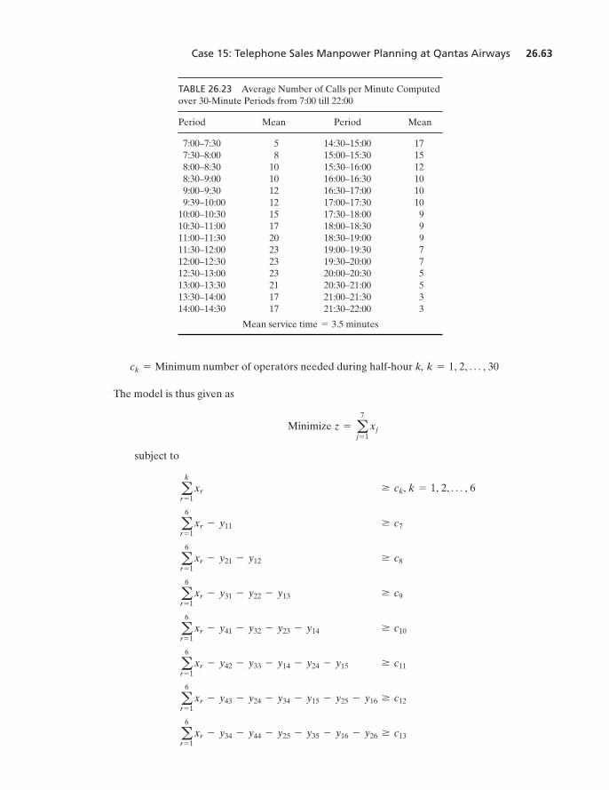
Case 15: Telephone Sales Manpower Planning at Qantas Airways 26.63
TABLE 26.23 Average Number of Calls per Minute Computedover 30-Minute Periods from 7:00 till 22:00
Period Mean Period Mean
7:00–7:30 5 14:30–15:00 177:30–8:00 8 15:00–15:30 158:00–8:30 10 15:30–16:00 128:30–9:00 10 16:00–16:30 109:00–9:30 12 16:30–17:00 109:39–10:00 12 17:00–17:30 10
10:00–10:30 15 17:30–18:00 910:30–11:00 17 18:00–18:30 911:00–11:30 20 18:30–19:00 911:30–12:00 23 19:00–19:30 712:00–12:30 23 19:30–20:00 712:30–13:00 23 20:00–20:30 513:00–13:30 21 20:30–21:00 513:30–14:00 17 21:00–21:30 314:00–14:30 17 21:30–22:00 3
Mean service time = 3.5 minutes
number of operators needed during half-hour k,
The model is thus given as
subject to
a6
r = 1xr - y34 - y44 - y25 - y35 - y16 - y26 Ú c13
a6
r = 1xr - y43 - y24 - y34 - y15 - y25 - y16 Ú c12
a6
r = 1xr - y42 - y33 - y14 - y24 - y15 Ú c11
a6
r = 1xr - y41 - y32 - y23 - y14 Ú c10
a6
r = 1xr - y31 - y22 - y13 Ú c9
a6
r = 1xr - y21 - y12 Ú c8
a6
r = 1xr - y11 Ú c7
ak
r = 1xr Ú ck, k = 1, 2, Á , 6
Minimize z = a7
j = 1xj
k = 1, 2, Á , 30ck = Minimum
M26_TAHA5937_09_SE_C26.QXD 7/26/10 9:27 PM Page 26.63
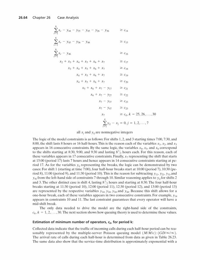
26.64 Chapter 26 Case Analysis
all and are nonnegative integers
The logic of the model constraints is as follows: For shifts 1, 2, and 3 starting times 7:00, 7:30, and8:00, the shift lasts 8 hours or 16 half-hours. This is the reason each of the variables and appears in 16 consecutive constraints. By the same logic, the variables and correspondto the shifts starting at 8:30, 9:00, and 9:30 and lasting hours each. For this reason, each ofthese variables appears in 17 consecutive constraints. Finally, representing the shift that startsat 15:00 (period 17) lasts 7 hours and hence appears in 14 consecutive constraints starting at pe-riod 17. As for the variables representing the breaks, the logic can be demonstrated by twocases: For shift 1 (starting at time 7:00), four half-hour breaks start at 10:00 (period 7), 10:30 (pe-riod 8), 11:00 (period 9), and 11:30 (period 10). This is the reason for subtracting and
from the left-hand side of constraints 7 through 10. Similar reasoning applies to for shifts 2 and 3. The other distinct case is shift 4, lasting hours and starting at 8:30. The four half-hourbreaks starting at 11:30 (period 10), 12:00 (period 11), 12:30 (period 12), and 13:00 (period 13)are represented by the respective variables and Because this shift allows for aone-hour break, each of these variables appears in two consecutive constraints. For example,appears in constraints 10 and 11. The last constraint guarantees that every operator will have amid-shift break.
The only data needed to drive the model are the right-hand side of the constraints,The next section shows how queuing theory is used to determine these values.
Estimation of minimum number of operators, , for period k:
Collected data indicate that the traffic of incoming calls during each half-hour period can be rea-sonably represented by the multiple-server Poisson queuing model The arrival rate of calls during each half-hour is determined from data as given in Table 26.23.The same data also show that the service-time distribution is approximately exponential with a
1M/M/c2 : 1GD/q /q2.
ck
ck, k = 1, 2, Á , 30.
y14
y44.y14, y24, y34,
8 1�2
yijy41
y11, y21, y31,
yij
x7
8 1�2
x6x4, x5,x3x1, x2,
yijxj
a4
i = 1yij - xj = 0, j = 1, 2, Á , 7
x7 Ú ck, k = 25, 26, Á , 30
x7 - y47 Ú c23
x7 - y37 Ú c23
x6 + x7 - y27 Ú c22
x5 + x6 + x7 - y17 Ú c21
x4 + x5 + x6 + x7 Ú c20
x4 + x5 + x6 + x7 Ú c19
x3 + x4 + x5 + x6 + x7 Ú c18
x2 + x3 + x4 + x5 + x6 + x7 Ú c17
a6
r = 1xr - y46 Ú c16
a6
r = 1xr - y45 - y36 - y46 Ú c15
a6
r = 1xr - y44 - y35 - y45 - y26 - y36 Ú c14
M26_TAHA5937_09_SE_C26.QXD 7/26/10 9:27 PM Page 26.64
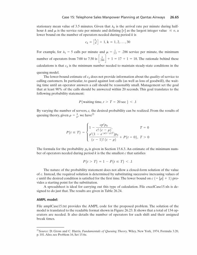
Case 15: Telephone Sales Manpower Planning at Qantas Airways 26.65
21Source: D. Gross and C. Harris, Fundamentals of Queuing Theory, Wiley, New York, 1974, Formula 3.20,p. 101. Also, see Problem 16, Set 15.6e.
stationary mean value of 3.5 minutes. Given that is the arrival rate per minute during half-hour k and is the service rate per minute and defining [v] as the largest integer value alower bound on the number of operators needed during period k is
For example, for calls per minute and service per minute, the minimum
number of operators from 7:00 to 7:30 is The rationale behind these
calculations is that is the minimum number needed to maintain steady-state conditions in the
queuing model.The lower-bound estimate of does not provide information about the quality of service to
calling customers. In particular, to guard against lost calls (as well as loss of goodwill), the wait-ing time until an operator answers a call should be reasonably small. Management set the goalthat at least 90% of the calls should be answered within 20 seconds. This goal translates to thefollowing probability statement:
By varying the number of servers, c, the desired probability can be realized. From the results ofqueuing theory, given we have21
The formula for the probability is given in Section 15.6.3. An estimate of the minimum num-ber of operators needed during period k is the the smallest c that satisfies
The nature of the probability statement does not allow a closed-form solution of the valueof c. Instead, the required solution is determined by substituting successive increasing values ofc until the desired condition is satisfied for the first time. The lower bound on pro-vides a starting point for the substitution.
A spreadsheet is ideal for carrying out this type of calculation. File excelCase15.xls is de-signed to do just that. The results are given in Table 26.24.
AMPL model:
File amplCase15.txt provides the AMPL code for the proposed problem. The solution of themodel is translated to the readable format shown in Figure 26.23. It shows that a total of 134 op-erators are needed. It also details the number of operators for each shift and their assignedbreak times.
c 1= [r] + 12
P5t 7 T6 = 1 - P5t … T6 6 .1
p0
P5t … T6 = d 1 -
cpcp0
c! 1c - r2, T = 0
rc11 - e-m1c -r2T2p0
1c - 12! 1c - r2 + P5t = 06, T 7 0
r =lm,
P5waiting time, t 7 T = 20 sec 6 6 .1
ck
ck
c 5.286 d + 1 = 17 + 1 = 18.
m =1
3.5 = .286l1 = 5
ck = Clkm D + 1, k = 1, 2, Á , 30
… v,m
lk
M26_TAHA5937_09_SE_C26.QXD 7/26/10 9:27 PM Page 26.65
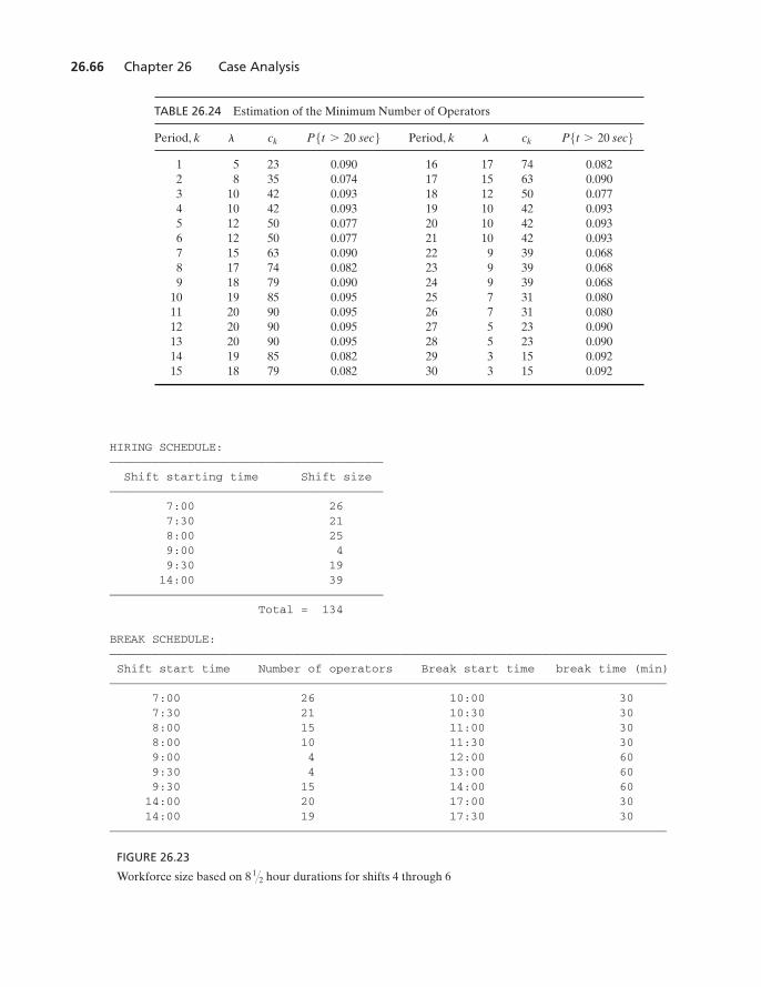
26.66 Chapter 26 Case Analysis
TABLE 26.24 Estimation of the Minimum Number of Operators
Period, k Period, k
1 5 23 0.090 16 17 74 0.0822 8 35 0.074 17 15 63 0.0903 10 42 0.093 18 12 50 0.0774 10 42 0.093 19 10 42 0.0935 12 50 0.077 20 10 42 0.0936 12 50 0.077 21 10 42 0.0937 15 63 0.090 22 9 39 0.0688 17 74 0.082 23 9 39 0.0689 18 79 0.090 24 9 39 0.068
10 19 85 0.095 25 7 31 0.08011 20 90 0.095 26 7 31 0.08012 20 90 0.095 27 5 23 0.09013 20 90 0.095 28 5 23 0.09014 19 85 0.082 29 3 15 0.09215 18 79 0.082 30 3 15 0.092
P5t 7 20 sec6cklP5t 7 20 sec6ckl
HIRING SCHEDULE:——————————————————————————————————————-Shift starting time Shift size
——————————————————————————————————————-7:00 267:30 218:00 259:00 49:30 1914:00 39
——————————————————————————————————————-Total = 134
BREAK SCHEDULE:——————————————————————————————————————————————————————————————————————————————-Shift start time Number of operators Break start time break time (min)——————————————————————————————————————————————————————————————————————————————-
7:00 26 10:00 307:30 21 10:30 308:00 15 11:00 308:00 10 11:30 309:00 4 12:00 609:30 4 13:00 609:30 15 14:00 6014:00 20 17:00 3014:00 19 17:30 30
——————————————————————————————————————————————————————————————————————————————-
FIGURE 26.23
Workforce size based on hour durations for shifts 4 through 68 1�2
M26_TAHA5937_09_SE_C26.QXD 7/26/10 9:27 PM Page 26.66
Questions:
1. An interesting question arises regarding the current practice of requiring dura-tion for shifts 4, 5, and 6 (starting at 8:30, 9:00, and 9:30, respectively) together with 1-hourbreaks. Preference among most employees is for the shorter shift (8 hours) with a half-hour break rather than the longer shift with a full-hour break. Study theimpact of imposing uniform 8-hour shifts with half-hour breaks for all employees.
2. Study the sensitivity of the solution to changing the probability of a 20-second delay inanswering a call.
A8 1�2 hours B
8 1�2-hour
Case 15: Telephone Sales Manpower Planning at Qantas Airways 26.67
M26_TAHA5937_09_SE_C26.QXD 7/26/10 9:27 PM Page 26.67

M26_TAHA5937_09_SE_C26.QXD 7/26/10 9:27 PM Page 26.68