Embed Size (px)
Citation preview

M1GLA – lecture notes
as lectured by Prof. Liebeck
Imperial College London
Mathematics 2006/2007

ii

CONTENTS iii
Contents
1 Introduction 1
2 Geometry in two dimensions 3
2.1 Vector operations . . . . . . . . . . . . . . . . . . . . . . . . . . . . . 3
2.2 Lines . . . . . . . . . . . . . . . . . . . . . . . . . . . . . . . . . . . . 4
2.3 Triangles . . . . . . . . . . . . . . . . . . . . . . . . . . . . . . . . . . 6
2.4 Distances . . . . . . . . . . . . . . . . . . . . . . . . . . . . . . . . . 7
2.5 Dot product . . . . . . . . . . . . . . . . . . . . . . . . . . . . . . . . 7
2.6 Equation of a line . . . . . . . . . . . . . . . . . . . . . . . . . . . . . 8
2.7 Perpendicular distance . . . . . . . . . . . . . . . . . . . . . . . . . . 9
2.8 Two famous inequalities . . . . . . . . . . . . . . . . . . . . . . . . . 10
3 Linear inequalities 13
4 Conics 15
4.1 Transforming conics . . . . . . . . . . . . . . . . . . . . . . . . . . . . 18
4.1.1 Translation . . . . . . . . . . . . . . . . . . . . . . . . . . . . 18
4.1.2 Rotation . . . . . . . . . . . . . . . . . . . . . . . . . . . . . . 19
4.2 The Theory . . . . . . . . . . . . . . . . . . . . . . . . . . . . . . . . 20
4.3 Geometrical definition of conics . . . . . . . . . . . . . . . . . . . . . 22
5 Matrices and linear equations 25
5.1 Method – Gaussian elimination . . . . . . . . . . . . . . . . . . . . . . 27
6 Some applications of matrix algebra 37
6.1 Linear equations . . . . . . . . . . . . . . . . . . . . . . . . . . . . . . 37
6.2 Population Distribution . . . . . . . . . . . . . . . . . . . . . . . . . . 38
6.3 Matrices and Geometry . . . . . . . . . . . . . . . . . . . . . . . . . . 41
6.3.1 Rotation . . . . . . . . . . . . . . . . . . . . . . . . . . . . . . 41
6.3.2 Reflection . . . . . . . . . . . . . . . . . . . . . . . . . . . . . 41
6.3.3 Combining Transformations . . . . . . . . . . . . . . . . . . . 41
7 Inverses 43
7.1 Relation to linear equations . . . . . . . . . . . . . . . . . . . . . . . . 43
7.2 Finding inverses . . . . . . . . . . . . . . . . . . . . . . . . . . . . . . 44
7.3 Finding inverses in general . . . . . . . . . . . . . . . . . . . . . . . . 45

iv CONTENTS
8 Determinants 47
8.1 Properties . . . . . . . . . . . . . . . . . . . . . . . . . . . . . . . . . 48
8.2 Effects of row operations on determinant . . . . . . . . . . . . . . . . 49
8.3 n × n determinants . . . . . . . . . . . . . . . . . . . . . . . . . . . . 51
9 Eigenvalues and eigenvectors 53
9.1 Eigenvectors . . . . . . . . . . . . . . . . . . . . . . . . . . . . . . . . 53
9.2 How to find eigenvectors and eigenvalues . . . . . . . . . . . . . . . . 54
9.2.1 Back to Fibonacci . . . . . . . . . . . . . . . . . . . . . . . . 55
9.3 Diagonalization . . . . . . . . . . . . . . . . . . . . . . . . . . . . . . 56
9.3.1 Repeated eigenvalues . . . . . . . . . . . . . . . . . . . . . . . 60
10 Conics(again) and Quadrics 63
10.1 Reduction of conics . . . . . . . . . . . . . . . . . . . . . . . . . . . . 65
10.1.1 Orthogonal matrices . . . . . . . . . . . . . . . . . . . . . . . 67
10.2 Quadric surfaces . . . . . . . . . . . . . . . . . . . . . . . . . . . . . . 67
10.3 Linear Geometry in 3 dimensions . . . . . . . . . . . . . . . . . . . . . 70
10.4 Geometry of planes . . . . . . . . . . . . . . . . . . . . . . . . . . . . 70

1
Chapter 1
Introduction
Some Greek highlights

2

3
Chapter 2
Geometry in two dimensions
This means geometry in the plane. Based on the real numbers. Think of real numbers
as points on the real line.
Definition 2.1. R2 is the set of all ordered pairs (x1, x2) with x1, x2 real numbers.
Note: (1, 3) 6= (3, 1)
Call (x1, x2) a vector. Geometrically, vector (x1, x2) will be used to represent several
things:
• Point p in the plane with coordinates (x1, x2)
• Position vector −→OPline in direction
−→OP , length OP
• Any vector −→AB of the same direction as −→OP
Usually we write x = (x1, x2).
The origin or zero vector is O = (0, 0).
2.1 Vector operations
Definition 2.2.
1) Addition
define the sum of two vectors by
(x1, x2) + (y1, y2) = (x1 + y1, x2 + y2)
2) Scalar multiplication
A scalar is a real number. If x = (x1, x2) is a vector and λ ∈ R is a scalar
λx = λ(x1, x2) = (λx1, λx2)
• Subtraction
x − y = x + (−y) = (x1 − y1, x2 − y2)

4 2.2. LINES
Note. If λ, ν ∈ R and x, y ∈ R2
i) λ(x + y) = λx + λy
ii) (λ+ ν)x = λx + νx
Proof.
(i)
λ(x + y) = λ(x1 + y1, x2 + y2)
= (λ(x1 + y1), λ(x2 + y2))
= (λx1 + λy1, λx2 + λy2)
= (λx1, λy1) + (λy1, λy2)
= λx + λy
(ii) excercise
�
2.2 Lines
In Euclid, points and lines are undefined. But we need to define points and lines. We
have already defined points.
Definition 2.3. Let a, u be vectors in R2 with u 6= O. The set of vectors {a+λu | λ ∈R} is called a line.
Definition 2.4. Two lines {a + λu | λ ∈ R} and {b + λv | λ ∈ R} are parallel iffv = αu for some α ∈ R.
Next we will prove the three famous propositions from Euclid.
Proposition 2.1. If L, L′ are parallel lines which have a point in common, then L = L′.
Proposition 2.2. Through any two points, there is exactly one line.
Proposition 2.3. Two non parallel lines meet in exactly one point.
Proof. Proposition 2.1.
Let
L = {a + λu | λ ∈ R}L′ = {b + λv | λ ∈ R}
As L, L′ are parallel, v = αu for some scale α ∈ R, so
L′ = {b + λαu | λ, α ∈ R} = {b + νu | ν ∈ R}

2.2. LINES 5
Given that L and L′ have x in common, we have
x = a + λ1u = b + λ2u λ1, λ2 ∈ Rb = a + λ1u − λ2u= a + (λ1 − λ2)u
b = a + λ3u (λ3 = (λ1 − λ2)→ λ3 ∈ R)Finally, we get
L′ = {b + λu | λ ∈ R}= {a + λ3u + λu | λ ∈ R}= {a + (λ3 + λ)u | λ ∈ R}= {a + λu | λ ∈ R}= L
�
Proof. Proposition 2.2.
Let u, v ∈ R2 to be our two points. Let us take the lineL = {u + λ(v − u) | λ ∈ R}
Suppose now that L′ is some line through u and v
L′ = {a + λw | λ ∈ R}Since points u and v line on L′, we get
u = a + λ1w
v = a + λ2w
v − u = (λ2 − λ1)wTherefore, lines L and L′ are parallel. As they also have a common point, they are (byproposition 1) identical.
�
Example 2.1. Find common point of
L1 = {(0, 1) + λ(1, 1) | λ ∈ R}L2 = {(4, 0) + λ(2, 1) | λ ∈ R}
By Proposition 3, there exists a unique common point, call it x .
x = (0, 1) + λ1(1, 1)
x = (4, 0) + λ2(2, 1)
Writing equations for individual coordinates, we get
0 + λ1 = 4 + 2λ2
1 + λ1 = 0 + λ2
−1 = 4 + λ2
λ2 = −5λ1 = 4 + 2(−5)λ1 = −6

6 2.3. TRIANGLES
Therefore
x = (0, 1)− 6(1, 1) = (−6,−5)= (4, 0)− 5(2, 1) = (−6,−5)
2.3 Triangles
Definition 2.5. A triangle is a set of 3 non-colinear points {a, b, c | a, b, c ∈ R2}.Edges of a triangle are the line segments ab, ac, bc, where
ab = {a + λ(b − a) | 0 ≤ λ ≤ 1}
Midpoint of ab is the point
a +1
2(b − 1) = 1
2(a + b)
A median of a triangle is a line joining one of a, b, c with the midpoint of the oposite
side (line segment).
Proposition 2.4. The 3 medians of a triangle meet in a common point.
Proof. Let the three medians be Ma, Mb and Mc
Ma = {a + λ(12(b + c)− a) | λ ∈ R}
Mb = {b + λ(12(a + c)− b) | λ ∈ R}
Mc = {c + λ(12(a + b)− c) | λ ∈ R}
We just show, that for λ = 23 , medians meet at the same point
Ma = a +1
3b +1
3c − 23a =1
3(a + b + c)
Mp = b +1
3a +1
3c − 23b =1
3(a + b + c)
Ma = c +1
3a +1
3b − 23c =
1
3(a + b + c)
Therefore, all the medians contain the point (sometimes called centroid) 13(a+ b+ c).
�
Note. Other interesting properties of triangles are
• 3 altitudes meet at a point (sometimes called orthocentre)
• 3 perpendicular bisectors meet at a point (sometimes called circumcentre)
• the 3 centres (orthocentre, circumcentre, centroid) are colinear, (they lie on Eulerline)

2.4. DISTANCES 7
2.4 Distances
Definition 2.6. The length of a vector x = (x1, x2) (denoted ‖x‖) is a real number
‖x‖ =√
x21 + x22
The distance between x and y (x, y ∈ R2) is the length of (x − y) called dist(x, y)
dist(x, y) =√
(x1 − y1)2 + (x2 − y2)2
2.5 Dot product
Definition 2.7. For x, y ∈ R2, dot product (scalar product) of x and y is a real number
x.y = x1y1 + x2y2
Example 2.2. x = (1, 2), y = (−1, 0)
‖x‖ =√
12 + 22 =√5
dist(x, y) =√
22 + 22 = 2√2
x.y = −1 + 0 = −1
Proposition 2.5. (i) ‖x‖2 + ‖y‖2 − ‖x − y‖2 = 2x.y
(ii) If θ is the angle between x and y then x.y = ‖x‖‖y‖ cos θ
(iii) The position vectors of x and y are at right angles iff x.y = 0
Proof.
(i)
LHS = x21 + x22 + y
21 + y
22 − (y1 − x1)2 − (y2 − x2)2
= −(−2x1y1)− (−2x2y2)= 2x.y
(ii) From cosine rule
‖x‖2 + ‖y‖2 − ‖y − x‖22‖x‖‖y‖ = cos θ
Using part (i), we get
2x.y = 2‖x‖‖y‖ cos θx.y = ‖x‖‖y‖ cos θ
�

8 2.6. EQUATION OF A LINE
2.6 Equation of a line
Consider a line L = {a + λu | λ ∈ R}, u = (u1, u2), define n = (−u2, u1), so thatn.u = 0.
For any x ∈ L, x = a + λu
x.n = (a + λu).n = a.n + λu.n = a.n
x.n = a.n
Proposition 2.6. Let L = {a + λy | λ ∈ R}, n = (−u2, u1). Then
(i) Every x in L satisfies x.n = a.n
(ii) Every solution of x.n = a.n lies on L
Proof.
(ii) Suppose x.n = a.n (we need to show that x = a + λu, i.e. x − a = λu). Then(x − a).n = 0.Let y = x − a, and say y = (y1, y2). As y .n = 0
−y1u2 + y2u1 = 0
y2u1 = y1u2
So, y = y1u1(u1, u2) if u1 6= 0, or y = y2
u2(u1, u2) if u2 6= 0.
Therefore
y = λu = x − ax = a + λu ∈ L
�
Definition 2.8. For a line L = {a + λu | λ ∈ R}, the vector n = (−u2, u1) (or anyscalar multiple of it) is called a normal to L.
The equation x.n = a.n is called the equation of L.
Proposition 2.7. The linear equation px1 + qx2 + r = 0 (1) is an equation of a line
with normal (p, q) and with direction (−q, p).
Proof.
Suppose q 6= 0. Then the solution of (1)p
qx1 + x2 +
r
q= 0
Let x1 = λ, x2 =−rq −
pλq , so
(x1, x2) =
(
λ,− rq− pλq
)
=
(
0,−rq
)
+ λ
(
1,−pq
)
which is a line with direction vector(
1, −pq
)
= 1−q (−q, p). Normal is clearly
(p, q).

2.7. PERPENDICULAR DISTANCE 9
When q = 0. Equation (1) is px1 + r = 0, with solution
(x1, x2) =
(−rp, 0
)
+ λ(0, 1)
Which is clearly a line with equation 1p (0, p) =1p (−q, p).
�
Definition 2.9. Lines L1 = {a + λu | λ ∈ R} and L2 = {b + λv | λ ∈ R} areperpendicular iff u.v = 0.
Proposition 2.8. Let lines L1, L2 have equations
L1 : p1x1 + q1x2 + r1 = 0
L2 : p2x1 + q2x2 + r2 = 0
Then
(i) L1, L2 are parallel iff (p1, q1) = α(p2, q2) for some scalar λ
(ii) L1, L2 are perpendicular iff (p1, q1) · (p2, q2) = 0
Proof.
(i) By Proposition 2.7
L1 = {a + λ(−q1, p1) | λ ∈ R}L2 = {b + λ(−q2, p2) | λ ∈ R}
These are parallel iff ∃α ∈ R such that (−q2, p2) = α(−q1, p1), i.e. α(p1, q1) =(p2, q2).
(ii) excercise
�
2.7 Perpendicular distance
Definition 2.10. For a line L and point p, p /∈ L, dist(p, L) is the length of the
perpendicular from p to L.
Proposition 2.9. If a is a point on the line and n is a normal to the line, then
dist(p, L) =
∣∣∣∣
(p − a).n‖n‖
∣∣∣∣
Note. A unit vector is a vector of length 1. If w is any vector, then w = w‖w‖ is a unit
vector. Therefore we can write
dist(p, l) = |(p − a).n|

10 2.8. TWO FAMOUS INEQUALITIES
Proof.
dist(p, L) = |‖p − a‖ cos θ|
=
∣∣∣∣
‖p − a‖‖n‖ cos θ‖n‖
∣∣∣∣
=
∣∣∣∣
(p − a).n‖n‖
∣∣∣∣
�
2.8 Two famous inequalities
Proposition 2.10. (Cauchy - Schwartz inequality)
Let x, y ∈ R2.
(i) |x.y | ≤ ‖x‖‖y‖
(ii) If |x.y | = ‖x‖‖y‖ then one of x.y is a scalar multiple of the other
Proof.
(i)
|x.y | ≤ ‖x‖‖y‖↔
(x1y1 + x2y2)2 ≤ (x21 + x
22 )(y
21 + y
22 )
↔x21 y
21 + 2x1y1x2y2 + x
22y22 ≤ x21y
21 + x
21y22 + x
22y21 + x
22 y22
↔0 ≤ x21y
22 + x
22y21 − 2x1y1x2y2
↔(x1y2 − x2y1)2 ≥ 0
(ii) If |x.y | = ‖x‖‖y‖, above proof shows
0 = x1y2 − x2y1x1x2=y1y2
Therefore one of x and y is a scalar multiple of the other.
Note that x.x = (x21 + x22 ) = ‖x‖2.
�
Proposition 2.11. (Triangle inequality) If x, y ∈ R2, then
‖x + y‖ ≤ ‖x‖+ ‖y‖

2.8. TWO FAMOUS INEQUALITIES 11
Proof.
‖x + y‖2 = (x + y)(x + y) = x.x + y .y + 2x.y
= ‖x‖2 + ‖y‖2 + 2x.y≤ ‖x‖2 + ‖y‖2 + 2‖x‖‖y‖ by Cauchy - Schwartz
≤ (‖x‖+ ‖y‖)2
Therefore ‖x + y‖ ≤ ‖x‖+ ‖y‖.�

12 2.8. TWO FAMOUS INEQUALITIES

13
Chapter 3
Linear inequalities

14

15
Chapter 4
Conics
In R2, a linear equation px1 + qx2 + r = 0 defines a line. Now we define a curve in R2
by quadratic equation.
Example 4.1. Circle of center c, radius r . It contains all the points x such that
‖x − c‖ = r
‖x − c‖2 = r2
(x1 − c1)2 + (x2 − c2)2 = r2
x21 + x22 − 2c2x2 + c21 + c22 − r2 = 0
Definition 4.1. A conic section in R2 is the set of poitns x ∈ R2, x = (x1, x2),satisfying a quadratic equation
ax21 + bx22 + cx1x2 + dx1 + ex2 + f = 0 (4.1)
where not all of a, b and c are 0.
Here are some basic examples
(1)
x21a2+x22b2= 1
is an ellipse
b
a
(2)
x21a2− x
22
b2= 1
is a hyperbola

16
(3)
x2 = ax21 + b
(a 6= 0) is a parabola.
b
(4)x21a2− x
22
b2= 0
is a pair of lines.
(5)x21a2= 1
is a pair of lines.

17
a−a
(6)x21a2= 0
is a double line
(7)x21a2+x22b2= 0
is a point
(8)x21a2+x22b2= −1
is the empty set (empty conic)
We call the conics (6), (7) and (8) degenerate conics. We’ll see how to reduce an
arbitrary conic to one of these basic examples.
18 4.1. TRANSFORMING CONICS
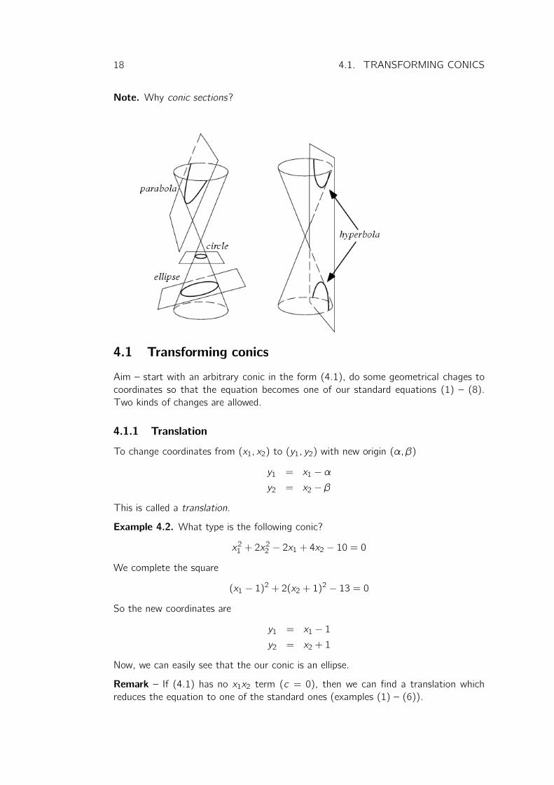
Note. Why conic sections?
4.1 Transforming conics
Aim – start with an arbitrary conic in the form (4.1), do some geometrical chages to
coordinates so that the equation becomes one of our standard equations (1) – (8).
Two kinds of changes are allowed.
4.1.1 Translation
To change coordinates from (x1, x2) to (y1, y2) with new origin (α, β)
y1 = x1 − αy2 = x2 − β
This is called a translation.
Example 4.2. What type is the following conic?
x21 + 2x22 − 2x1 + 4x2 − 10 = 0
We complete the square
(x1 − 1)2 + 2(x2 + 1)2 − 13 = 0
So the new coordinates are
y1 = x1 − 1y2 = x2 + 1
Now, we can easily see that the our conic is an ellipse.
Remark – If (4.1) has no x1x2 term (c = 0), then we can find a translation which
reduces the equation to one of the standard ones (examples (1) – (6)).

4.1. TRANSFORMING CONICS 19
4.1.2 Rotation
Rotate axes anticlockwise through θ. What happens to the coordinates of a general
point P?
Say P has old coordinates (x1, x2) and new coordinates (y1, y2).
θ
α
r y1
x1
x2
y2
bP
Now
y1 = r cosα
y2 = r sinα
and
x1 = r cos(α+ θ)
x2 = r sin(α+ θ)
Hence
x1 = r cos θ cos θ − r sinα sin θ= y1 cos θ − y2 sin θ
and
x2 = r sinα cos θ + cosα sin θ
= y2 cos θ + y1 sin θ
Summarizing – change of coordinates when we do a rotation through angle θ is
x1 = y1 cos θ − y2 sin θx2 = y1 sin θ + y2 cos θ

20 4.2. THE THEORY
Example 4.3. Rotation through π4 .
x1 =1√2(y1 − y2)
x2 =1√2(y1 + y2)
Example 4.4. What is the following conic (find the rotation and translation to change
coordinates and get standard equation)
x21 + x22 + 4x1x2 = 1
(From the hat method) Let’s rotate through π4 . By magic (see later). Then our
equation becomes
1
2(y1 − y2)2 +
1
2(y1 + y2)
2 + 41
2(y1 − y2)(y1 + y2) = 1 3y21 − y22 = 1
This is a hyperbola.
4.2 The Theory
Start with general conic
ax21 + bx22 + cx1x2 + dx1 + ex2 + f = 0
Aim
(i) find the rotation which gets rid of x1x2
(ii) complete the square to find the translation which changes the equation to one
of our six standard equations
Part(i).
If c = 0, we don’t need to rotate. So assume that c 6= 0. When we do general rotationthrough θ we change coordinates to y1, y2
x1 = y1 cos θ − y2 sin θx2 = y1 sin θ + y2 cos θ
We aim to find θ so that the new equation has no y1y2 term.
ax21 = a(y1 cos θ − y2 sin θ)2
bx22 = b(y1 sin θ + y2 cos θ)2
cx1x2 = c(y1 sin θ + y2 cos θ)(y1 cos θ − y2 sin θ)
So the y1y2 term when we change coordinates will be
−2a sin θ cos θ + 2b sin θ cos θ + c(cos2 θ − sin2 θ)=
(b − a) sin 2θ + c cos 2θ
4.2. THE THEORY 21
So we want to choose θ to make this expression zero.
(a − b) sin 2θ = c cos 2θ
If a 6= b then
tan 2θ =c
a − bIf a = b, we want to cos 2θ = 0, so take θ = π
4 .
Summary
• Step 1 – Rotation. If c 6= 0 in (4.1), we rotate through θ, where
θ =π
4
when a = b or
tan 2θ =c
a − bwhen a 6= b.
• Step 2 – Translation. After Step 1, equation becomesa′y21 + b
′y22 + d′y1 + e
′y2 + f′ = 0
Now we complete the square to find a translation which changes equation to one
of the standard ones.
We’ve proved:
Theorem 4.1. Every conic in the form (4.1) can be changed by rotation and translation
of the axes to one of the standard equations (1) – (8). Thus every conic is either an
ellipse, hyperbola, parabola, or one of the degenerate conics.
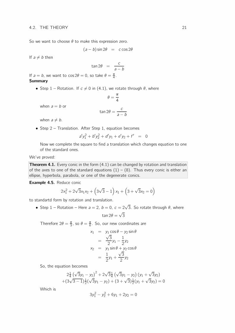
Example 4.5. Reduce conic
2x21 + 2√3x1x2 +
(
3√3− 1
)
x1 +(
3 +√3x2 = 0
)
to standartd form by rotation and translation.
• Step 1 – Rotation – Here a = 2, b = 0, c = 2√3. So rotate through θ, where
tan 2θ =√3
Therefore 2θ = π3 , so θ =
π6 . So, our new coordinates are
x1 = y1 cos θ − y2 sin θ
=
√3
2y1 −
1
2y2
x2 = y1 sin θ + y2 cos θ
=1
2y1 +
√3
2y2
So, the equation becomes
214(√3y1 − y2
)2+ 2√314(√3y1 − y2
)(y1 +
√3y2)
+(3√3− 1)12(
√3y1 − y2) + (3 +
√3)12(y1 +
√3y2) = 0
Which is
3y21 − y22 + 6y1 + 2y2 = 0
22 4.3. GEOMETRICAL DEFINITION OF CONICS
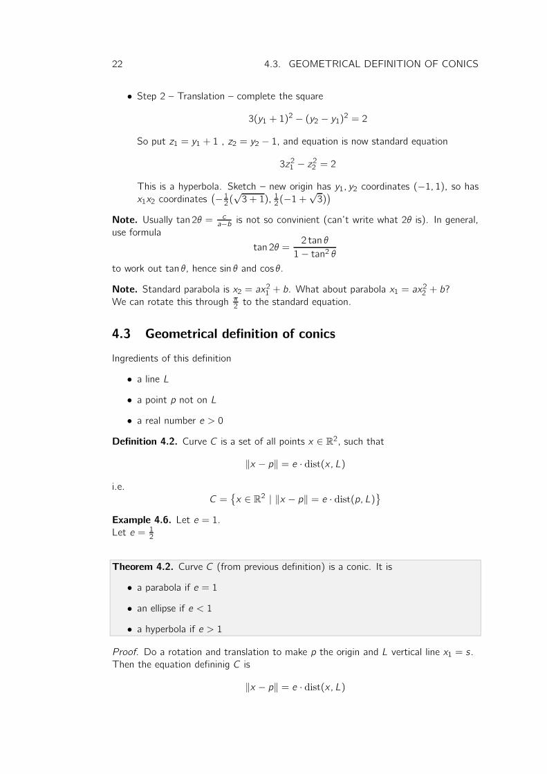
• Step 2 – Translation – complete the square
3(y1 + 1)2 − (y2 − y1)2 = 2
So put z1 = y1 + 1 , z2 = y2 − 1, and equation is now standard equation
3z21 − z22 = 2
This is a hyperbola. Sketch – new origin has y1, y2 coordinates (−1, 1), so hasx1x2 coordinates
(−12(√3 + 1), 12(−1 +
√3))
Note. Usually tan 2θ = ca−b is not so convinient (can’t write what 2θ is). In general,
use formula
tan 2θ =2 tan θ
1− tan2 θto work out tan θ, hence sin θ and cos θ.
Note. Standard parabola is x2 = ax21 + b. What about parabola x1 = ax
22 + b?
We can rotate this through π2 to the standard equation.
4.3 Geometrical definition of conics
Ingredients of this definition
• a line L
• a point p not on L
• a real number e > 0
Definition 4.2. Curve C is a set of all points x ∈ R2, such that
‖x − p‖ = e · dist(x, L)
i.e.
C ={x ∈ R2 | ‖x − p‖ = e · dist(p, L)
}
Example 4.6. Let e = 1.
Let e = 12
Theorem 4.2. Curve C (from previous definition) is a conic. It is
• a parabola if e = 1
• an ellipse if e < 1
• a hyperbola if e > 1
Proof. Do a rotation and translation to make p the origin and L vertical line x1 = s .
Then the equation defininig C is
‖x − p‖ = e · dist(x, L)

4.3. GEOMETRICAL DEFINITION OF CONICS 23
i.e
‖x‖ = e · |x1 − s |i.e
‖x‖2 = e2(x1 − s)2
i.e
x21 + x22 = e
2(x21 − 2sx1 + s2)i.e
x21 (1− e2) + x22 + 2se2x1 − s2e2 = 0If e = 1, the x21 term vanishes – this is a parabola.
Now suppose e 6= 1.Complete square
(1− e2)(
x1 +se2
1− e2)2
+ x22 − s2e2 −s2e4
1− e2 = 0
So put y1 = x1 +se2
1−e2 and y2 = x2. Then get standard equation
(1− e2)y21 + y22 = s2e2(
1 +e2
1− e2)
i.e
y21 +y221− e2 =
s2e2
(1− e2)2 (4.2)
If e < 1, this is an ellipse. If e > 1, this is hyperbola. �
Definition 4.3. The conic has focus p, directric L, excentricity e from the previous
proof.
Example 4.7. Find e, p and L for the ellipse
x212+ x22 = 1
This is the standard equation. We compare it with (4.2)
y21 +y221− e2 =
s2e2
(1− e2)2 (4.3)
From the y coordinate picture, the focus is(se2
1−e2 , 0)
, directrix is x1 = s +se2
1−e2 .
Compare equations
y21 +y221− e2 =
s2e2
(1− e2)2x21 + 2x
22 = 2
So,
1
1− e2 = 2
s2e2
(1− e2)2 = 2
So e = 1√2, s = 1. So the excentricity is 1√
2, focus (1, 0) and the directrix is x1 = 2.
Note. Ellipse has in fact two foci ±p, and two directrices L, L′.

24 4.3. GEOMETRICAL DEFINITION OF CONICS

25
Chapter 5
Matrices and linear equations
Definition 5.1. The space Rn – define
R1 = R
R2 = set of ordered pairs
R3 = set of all triples
R4 = set of all quadruples
In general, Rn is the set of all n-tuples (x1, x2, . . . , xn) with x1 ∈ R. Call these n-tuplesvectors.
Note that Ri 6⊆ Ri+1.
The Rn has interesting structure
• geometric – points, lines, curves
• algebraic
Definition 5.2. Addition of vectors
(x1, x2, . . . , xn) + (y1, y2, . . . , yn) = (x1 + y1, . . . , xn + yn)
Scalar multiplication
λ(x1, . . . , xn) = (λx1, . . . , λxn)
Definition 5.3. A linear equation in x1, x2, . . . xn is
a1x1 + a2x2 + · · ·+ anxn = b
where coefficients ai , b ∈ R.
Definition 5.4. A solution to a linear equation is a vector (k1, . . . , kn) such that the
equation is satisfied when we put xi = ki .
Example 5.1. (1,−2, 3) is a solution to the linear equation x1 + x2 + x3 = 2.
Definition 5.5. A system of linear equations in x1, . . . xn is a collection of one or more
linear equations in these variables.
Example 5.2.
26
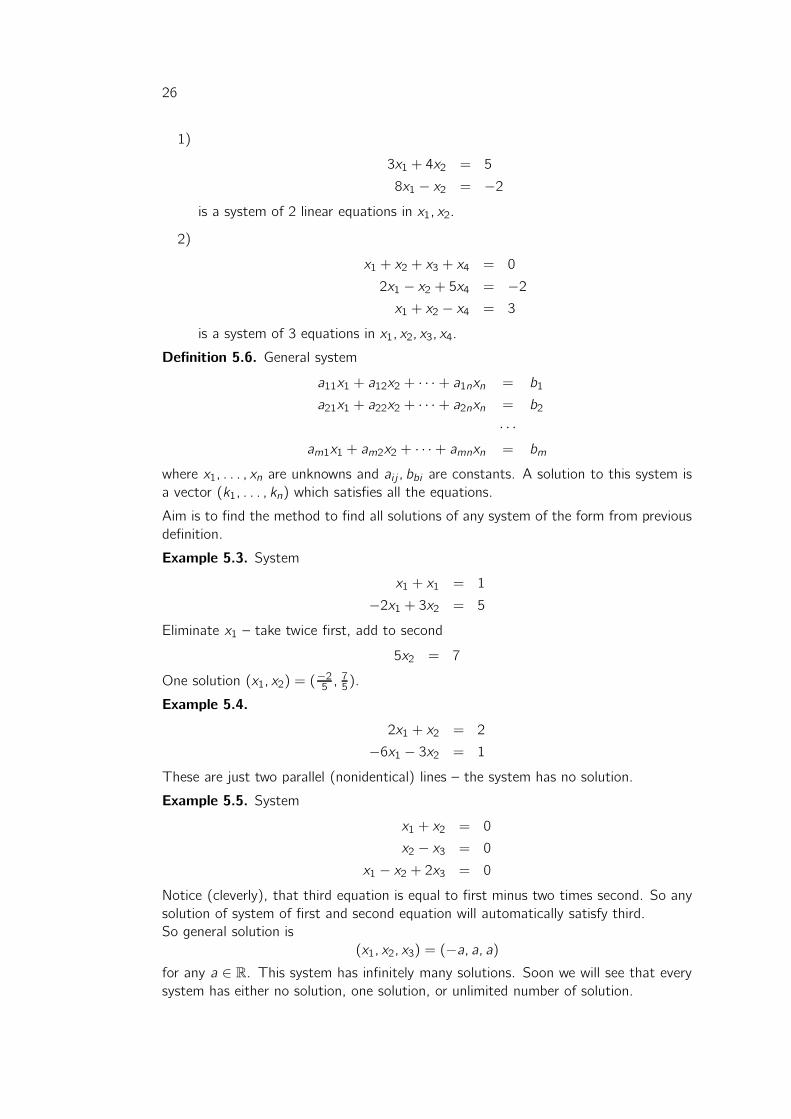
1)
3x1 + 4x2 = 5
8x1 − x2 = −2is a system of 2 linear equations in x1, x2.
2)
x1 + x2 + x3 + x4 = 0
2x1 − x2 + 5x4 = −2x1 + x2 − x4 = 3
is a system of 3 equations in x1, x2, x3, x4.
Definition 5.6. General system
a11x1 + a12x2 + · · · + a1nxn = b1
a21x1 + a22x2 + · · · + a2nxn = b2
· · ·am1x1 + am2x2 + · · ·+ amnxn = bm
where x1, . . . , xn are unknowns and ai j , bbi are constants. A solution to this system is
a vector (k1, . . . , kn) which satisfies all the equations.
Aim is to find the method to find all solutions of any system of the form from previous
definition.
Example 5.3. System
x1 + x1 = 1
−2x1 + 3x2 = 5
Eliminate x1 – take twice first, add to second
5x2 = 7
One solution (x1, x2) = (−25 ,75).
Example 5.4.
2x1 + x2 = 2
−6x1 − 3x2 = 1
These are just two parallel (nonidentical) lines – the system has no solution.
Example 5.5. System
x1 + x2 = 0
x2 − x3 = 0
x1 − x2 + 2x3 = 0
Notice (cleverly), that third equation is equal to first minus two times second. So any
solution of system of first and second equation will automatically satisfy third.
So general solution is
(x1, x2, x3) = (−a, a, a)for any a ∈ R. This system has infinitely many solutions. Soon we will see that everysystem has either no solution, one solution, or unlimited number of solution.

5.1. METHOD – GAUSSIAN ELIMINATION 27
5.1 Method – Gaussian elimination
Example 5.6. System
x1 + 2x2 + 3x3 = 9
4x1 + 5x2 + 6x3 = 24
3x1 + x2 − 2x3 = 4
Step 1 – Eliminate x1 from second and third, using first. We get equivalent system
x1 + 2x2 + 3x3 = 9
−3x2 − 6x3 = −12 (2)− 4(1)−5x2 − 11x2 = −23 (3)− 3(1)
This system has the same solutions as the original one as new equations are combina-
tions of orignal ones, and vice versa.
Step 2 – Eliminate x2 from the third equation using only second equation.
x1 + 2x2 + 3x3 = 9
−3x2 − 6x3 = −12−x3 = −3 (3)− 5
3(2)
Step 3 – Solve!
By third, x3 = 3. By the second, 3x2 = 12− 18, so x2 = −2. By the first, x1 = 4. Sothe system has one solution (4,−2, 3).
For bigger systems, we need better notation. This is provided by matrices.
Definition 5.7. A matrix is a rectangular array of numbers. Eg
(1 2 3
4 5 6
)
This is 2× 3 matrix.
1
5
−π
This is 3× 1 matrix.Call matrix m×n if it has m rows, n collumns. We use matrices to encapsulate systemsof linear equations. System from previous example has the coefficients matrix
1 2 3
4 5 6
3 1 −2
and augmented matrix
1 2 3 9
4 5 6 24
3 1 −2 4
28 5.1. METHOD – GAUSSIAN ELIMINATION
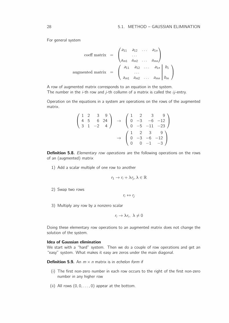
For general system
coeff matrix =
a11 a12 . . . a1n. . .
am1 am2 . . . amn
augmented matrix =
a11 a12 . . . a1n b1. . .
am1 am2 . . . amn bm
A row of augmented matrix corresponds to an equation in the system.
The number in the i-th row and j-th collumn of a matrix is called the i j-entry.
Operation on the equations in a system are operations on the rows of the augmented
matrix.
1 2 3 9
4 5 6 24
3 1 −2 4
→
1 2 3 9
0 −3 −6 −120 −5 −11 −23
→
1 2 3 9
0 −3 −6 −120 0 −1 −3
Definition 5.8. Elementary row operations are the following operations on the rows
of an (augmented) matrix
1) Add a scalar multiple of one row to another
r1 → ri + λrj , λ ∈ R
2) Swap two rows
ri ↔ rj
3) Multiply any row by a nonzero scalar
ri → λri , λ 6= 0
Doing these elementary row operations to an augmented matrix does not change the
solution of the system.
Idea of Gaussian elimination
We start with a “hard” system. Then we do a couple of row operations and get an
“easy” system. What makes it easy are zeros under the main diagonal.
Definition 5.9. An m × n matrix is in echelon form if
(i) The first non-zero number in each row occurs to the right of the first non-zero
number in any higher row
(ii) All rows (0, 0, . . . , 0) appear at the bottom.

5.1. METHOD – GAUSSIAN ELIMINATION 29
Example 5.7. The following matrices
1 2 3 9
0 −3 −6 −120 0 −3 −9
(0 0 1
0 0 0
)
are in echelon form. This one is not
0 1 3
1 0 0
0 0 0
The point If a system has its augmented matrix in echelon form, the system is easy
to solve.
Example 5.8. Solve the system of equations with augmentated matrix
2 −1 3 00 1 1 1
0 0 0 0
This system is
2x1 − x2 + 3x3 = 0
x2 + x3 = 1
Solve from bottom up. Equation 3 tells us nothing. Let x3 = a (any a ∈ R. Then eq2 implies that x2 is 1− a.Equation 1 implies 2x1 = x2 − 3x2, therefore x1 = 1−4a
2 .
Therefore the solutions are (x1, x2, x3) = (12(1 − 4a), 1 − a, a). E.g when a = 0, we
get solution(12 , 1, 0
).
Example 5.9. Solve the system with augmentated matrix
2 −1 3 00 1 1 0
0 0 0 2
System thus is
2x1 − x2 + 3x3 = 0
x2 + x3 = 1
0 = 2
Third equation instantly implies no solution at all.

30 5.1. METHOD – GAUSSIAN ELIMINATION
Example 5.10.
1 1 1 3 2 4 0
0 0 0 2 −2 0 30 0 0 0 1 1 0
The system is
x1 + x2 + x3 + 3x4 + 2x5 + 4x6 = 0
2x4 − x5 = 3
x5 + x6 = 0
Equation 3 sets x6 = a (any a). Then x5 = −a. From 2 we get x4 = 12(x5 + 3) =
12(3− a). From 1 we get x3 = b and x2 = c. Then x1 = −c − b− 23(3− a) + 2a− 4a= −9
2 − 12a − b − c. The general solution is
(x1, x2, x3, x4, x5, x6)
=
(−92 − 12a − b − c, c, b, 12(3− a), a, a)
for any a, b, c ∈ R.
In general, if augmentated matrix is in echelon form, solve the system by solving the
last equation, then the next last, and so on.
This method is called back substitution.
The variables we can put free equal to a, d, c etc are free variables. E.g. in previous
example, the free variables are x6, x3, x2.
Theorem 5.1. (Gausian elimination theorem)
Any matrix can be reduced by elementary row operations to a matrix which is in echelon
form.
Method 5.1. (Gausian elimination method)
System of linear equations (augmented matrix). We put the augmented to echelon
form using elementary row operations. Solve the new system by back substitution.
Example 5.11. Solve the system with augmentation matrix
A =
1 0 3 2 5 1
1 0 3 5 8 1
1 1 4 5 7 0
1 −1 2 −1 3 3
Answer.
• Step 1 – clear first collumn using top left hand entry (i.e. equations 2, 3, 4 takeaway equation 1)
A→
1 0 3 2 5 1
0 0 0 3 3 0
0 1 1 3 2 −10 −1 −1 −3 −2 1
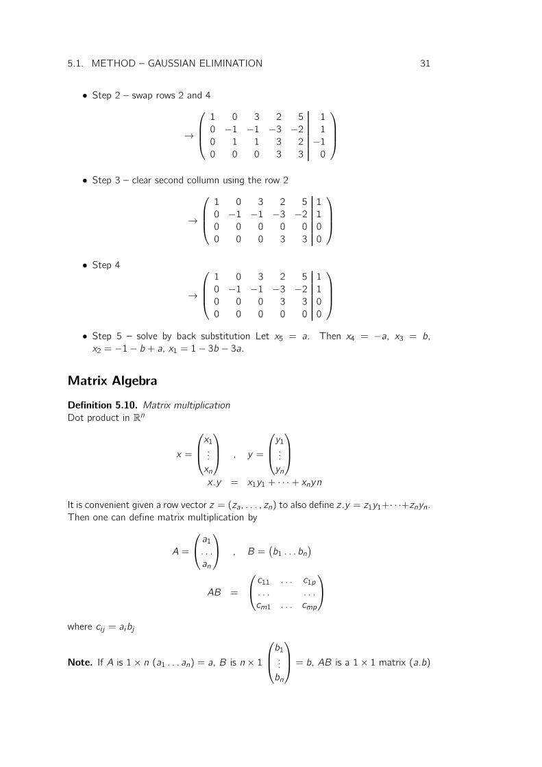
5.1. METHOD – GAUSSIAN ELIMINATION 31
• Step 2 – swap rows 2 and 4
→
1 0 3 2 5 1
0 −1 −1 −3 −2 1
0 1 1 3 2 −10 0 0 3 3 0
• Step 3 – clear second collumn using the row 2
→
1 0 3 2 5 1
0 −1 −1 −3 −2 10 0 0 0 0 0
0 0 0 3 3 0
• Step 4
→
1 0 3 2 5 1
0 −1 −1 −3 −2 10 0 0 3 3 0
0 0 0 0 0 0
• Step 5 – solve by back substitution Let x5 = a. Then x4 = −a, x3 = b,x2 = −1− b + a, x1 = 1− 3b − 3a.
Matrix Algebra
Definition 5.10. Matrix multiplication
Dot product in Rn
x =
x1...
xn
, y =
y1...
yn
x.y = x1y1 + · · ·+ xnyn
It is convenient given a row vector z = (za, . . . , zn) to also define z.y = z1y1+· · ·+znyn.Then one can define matrix multiplication by
A =
a1. . .
an
, B =(b1 . . . bn
)
AB =
c11 . . . c1p. . . . . .
cm1 . . . cmp
where ci j = aibj
Note. If A is 1× n (a1 . . . an) = a, B is n × 1
b1...
bn
= b, AB is a 1× 1 matrix (a.b)

32 5.1. METHOD – GAUSSIAN ELIMINATION
Key properties of matrix multiplication
1) One can multiply an m× n matrix A with an r × s matrix B iff r = n. Then, ABwill be an m × s matrix.
2) Commutativity fails, i.e. in general AB 6= BA.In order for both AB and BA to be defined, they must be square matrices of
same size, i.e. n × n for some n.
Example 5.12.
A =
(1 2
3 4
)
, B =
(0 1
−1 2
)
Then
AB =
(−2 5
−4 11
)
BA =
(3 4
5 6
)
3) Matrix multiplication, like for × on R, is associative.
Theorem 5.2. Given any matrices A m × n, B n × p, C p × q
(AB)C = A(BC)
Example 5.13.
A =
(1 2
3 4
)
, B =
(0 1
−1 2
)
, C =
(1 2
3 0
)
Then
AB =
(−2 5
−4 11
)
(AB)C =
(13 −429 −8
)
BC =
(3 0
5 −2
)
, A(BC) =
(13 −429 −8
)
Proof. First, we do special case, when C is p×1 matrix, i.e. column vector. LetA is m × n, B is n × p, x is p × 1. We show that
(AB)x = A(Bx)
Let y = Bx be a vector and z = Ay . So z is the right hand side. Claim is
z = (AB)x .
y = B x
(n × 1) (n × p) (p × 1)
y =
y1...
yn
=
b11 . . . b1p...
...
bn1 . . . bnp
x1...
xp

5.1. METHOD – GAUSSIAN ELIMINATION 33
z =
z1...
zm
=
a11 . . . a1n...
...
bm1 . . . bmn
y1...
yn
For i ≤ i ≤ n zi = ai1y1 + · · ·+ ainyn, yj = bj ix1 + · · ·+ bjpxp.Then
zi
=
ai1(b1ix1 + · · ·+ b1p) + ai2(b2ix1 + · · · + b2p)+. . .
+ain(bnix1 + · · ·+ bnp)
=
(ai1b11 + ai2b21 + · · ·+ ainbn1)x1 + (ai2b12 + ai2b22 + · · ·+ ainbn2)x2+ · · ·+ (ai2b1p + ai2b2p + · · ·+ ainbnp)xp
Thus coefficient of xi in zi is
(ai1bi j + ai2b2j + · · ·+ ainbnj)
which is ai .bj , where
ai =
ai1...
ain
, bj =
b1j...
bnj
which by definition is the (i , j) entry of AB!
Claim
(AB)C = A(BC)
Write C =
......
c1 cq...
...
Then
BC =(Bc1 . . . Bcq
)
Therefore
A(BC) =(A(Bc1) . . . A(Bcq)
)
�
4) Again, as for + and × on R, distributivity holds
Proposition 5.3. Given matrices A m × n, B, C, both n × p
A(B + C) = AB + AC

34 5.1. METHOD – GAUSSIAN ELIMINATION
Powers of matrices
Definition 5.11. A square matrix is one which is n × n for some n.If A is n × n, define
A2 = AA
A3 = (AA)A = A(AA)
A4 = A3A
. . .
An = An−1A
Example 5.14.
(1 2
0 1
)2
=
(1 2
0 2
)(1 2
0 2
)
=
(1 4
0 1
)
Definition 5.12. The identity matrix is
2× 2 I2 =(1 0
0 1
)
3× 3 I3 =
1 0 0
0 1 0
0 0 1
n × n In =
1 0 . . .
0 1 . . .
0 0.. .
0 0 0 1
Proposition 5.4. If A is m × n and B is n × p then
AIn = A
InB = B
Link between addition and multiplication
Proposition 5.5.
(i) If A is m × n and B, C are n × p, then
A(B + C) = AB + AC
(ii) If D, E are m × n and F is n × p, then
(D + E)F = DF + EF
Proof.
(i) Let A = (ai j), B = (bi j), C = (ci j). The i j-entry of AB is
(aj1 . . . ain)
bi j...
bnj
= ai1bi j + · · ·+ ainbnj

5.1. METHOD – GAUSSIAN ELIMINATION 35
So i j-entry of A(B + C) is
ai1(b1j + c1j) + · · ·+ ain(bnj + cnj)=
ai1b1j + ai1c1j + · · · + ainbnj + aincnj=
(ai1b1j + · · ·+ ainbnj) + (ai1c1j + · · ·+ aincnj)
This is the i j entry of AB + AC.
(ii) Left to enthusiastic reader. �

36 5.1. METHOD – GAUSSIAN ELIMINATION

37
Chapter 6
Some applications of matrixalgebra
6.1 Linear equations
We know that a general system of linear equations
a11x1 + · · ·+ a1nxn = b1...
am1x1 + · · ·+ amnxn = bn
can be expressed as a matrix product
Ax = b
where A =(ai j), x =
x1...
xn
and b =
b1...
bm
Proposition 6.1. The number of solutions of a system Ax = b is 0, 1 or ∞.Proof. Suppose the number of solutions is not 0 or 1, i.e. there are at least two
solutions. We prove that this implies that there are infinitely many solutions.
Let p and q be two different solutions (p, q ∈ Rn), soAp = b
Aq = b
and p 6= q. ThenA(p − q) = Ap − Aq = 0
For any scalar λ ∈ RAλ(p − q) = λA(p − q) = λ0
So
A(p + λ(p − q)) = Ap + Aλ(p − q) = Ap + 0 = bSo p + λ(p − q) is a solution of the original system.Since p 6= q, p − q 6= 0 and so each different scalar λ gives a different solution. Sothere are ∞ solutions. �

38 6.2. POPULATION DISTRIBUTION
Structure of solutions
Proposition 6.2.
(i) System Ax = 0 either has one solution (which must be x = O) or it has an
infinite number of solutions.
(ii) Suppose p is a solution of a system Ax = b (i.e. p ∈ Rn, Ap = b). Then allsolutions of Ax = b take the form
p + h
where h is a solution of the system Ax = 0.
Example 6.1. System
(1 0 3
0 1 1
)
x1x2x3
=
(2
1
)
. The general solution is
x = (2− 3a, 1− a, a)
Particular solution p = (2, 1, 0). So general solution is
(2− 3a, 1− a, a) = (2, 1, 0) + (−3a,−a, a) = p + h
Where h = (−3a,−a, a) is the general solution of(1 0 3
0 1 1
)
x =
(0
0
)
.
Proof.
(i) clear from previous proposition
(ii) Let q be a solution of A. So Ap = b, Aq = b. So A(q − p) = 0.Put q − p = h, a solution to Ax = 0. Then q = p + h.
�
6.2 Population Distribution
Example 6.2. Population classified in 3 income states
(1) Poor (P)
(2) Middle incom (M)
(3) Rich(R)
Over one generation (20 year period)
P → 20%M, 5%R rest stay P
M → 25%P, 10%R
R → 5%P, 30%M
6.2. POPULATION DISTRIBUTION 39
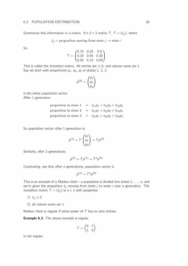
Summarize this information in a matrix. It’s 3× 3 matrix T , T = (ti j), where
ti j = proportion moving from state j → state i
So
T =
0.75 0.25 0.5
0.20 0.65 0.30
0.05 0.10 0.65
This is called the transition matrix. All entries are ≥ 0, and column sums are 1.Say we start with proportions p1, p2, p3 in states 1, 2, 3.
p(0) =
p1p2p3
is the initial population vector.
After 1 generation
proportion in state 1 = t11p1 + t12p2 + t13p3
proportion in state 2 = t21p1 + t22p2 + t23p3
proportion in state 3 = t31p1 + t32p2 + t33p3
So population vector after 1 generation is
p(1) = T
p1p2p3
= Tp(0)
Similarly, after 2 generations
p(2) = Tp(1) = T 2p(0)
Continuiing, see that after n generations, population vector is
p(n) = T np(0)
This is an example of a Markov chain – a population is divided into states 1, . . . , n, and
we’re given the proportion ti j moving from state j to state i over a generation. The
transition matrix T = (ti j) is n × n with properties
1) ti j ≥ 0
2) all column sums are 1
Markov chain is regular if some power of T has no zero entries.
Example 6.3. The above example is regular.
T =
(0 1
1 0
)
is not regular.

40 6.2. POPULATION DISTRIBUTION
Basic Fact
In a regular Markov chain, as n grows, the vector Tmp(0) gets closer and closer to a
steady state vector s =
s1s2...
sn
where
1) s1 + · · ·+ sn = 1
2) Ts = s
This is true, whatever the initial population vector p(0). Proof is not hard.
Example 6.4. On a desert island, a veg-prone community dies according to
(1) no-one eats meat 2 days in a row
(2) if someone doesn’t eat meat one day, they toss a coin: heads eat meat next day,
tails don’t
What proportion can be expected to eat meat on a given day?
Answer – Markov chain.
• State 1: meat
• State 2: no meat
• “generation”: 1 day
Transition matrix
T =
(0 1
2
1 12
)
Notice T 2 =
(12
14
12
34
)
. So it is regular. By our Basic Fact, we have a steady state
vector s =
(s1s2
)
, where s1 + s2 = 1 and Ts = s .
So
1
2s2 = s1
s1 +1
2s2 = s2
s1 + s2 = 1
So in long run, 13 of population will be eating meat on a given day.

6.3. MATRICES AND GEOMETRY 41
6.3 Matrices and Geometry
6.3.1 Rotation
Consider a rotation about the origin through angle θ. Then
y1 = r cos(θ + α)
= r(cos θ cosα− sin θ sinα)= x1 cos θ − x2 sin θ
y2 = r sin(θ + α)
= r(sin θ cosα+ cos θ sinα)
= x1 sin θ + x2 cos θ
So (y1y2
)
=
(cos θ − sin θsin θ cos θ
)(x1x2
)
Call Rθ =
(cos θ − sin θsin θ cos θ
)
, a rotation matrix.
6.3.2 Reflection
Let s be the reflection in the x1 axis sending
x =
(x1x2
)
→(x1x2
)
=
(1 0
0 −1
)(x1x2
)
So matrix S =
(1 0
0 −1
)
represents the reflection s .
6.3.3 Combining Transformations
Two rotations, say through θ then γ
x → rγ(rθ(x))
x → Rγ(Rθ(x))
= (RγRθ)x =
(cosγ − sin γsin γ cos γ
)(cos θ − sin θsin θ cos θ
)
= Rγ+θ
Reflection+Rotation
Now consider srθ, sending x → s(rθ(x)). This sendsx → S(Rθx)
= (SRθ)x
=
(1 0
0 −1
)(cos θ − sin θsin θ − cos θ
)
x
=
(cos − sin θ
− sin θ − cos θ
)
x

42 6.3. MATRICES AND GEOMETRY

43
Chapter 7
Inverses
Definition 7.1. Let A be a square matrix (n × n). Say another n × n matrix B is aninverse of A iff AB = BA = In.
Inverse of A is denoted A−1. If A has an inverse, A is invertible.
Example 7.1. A =
(1 1
0 1
)
. Then
(1 1
0 1
)(1 −10 1
)
=
(1 0
0 1
)
(1 −10 1
)(1 1
0 1
)
=
(1 0
0 1
)
Example 7.2.(1 2
0 0
)(a b
c d
)
=
(a + 2c b + 2d
0 0
)
which cannot equal to I.
Proposition 7.1. If A is invertible then its inverse is unique.
Proof. Suppose B, C are inverses of A. Then
AB = BA = I
AC = CA = I
B = BI = B(AC) = (BA)C = IC = C
�
7.1 Relation to linear equations
Proposition 7.2. Suppose A is invertible. Then any system Ax = b has a unique
solution
x = A−1b

44 7.2. FINDING INVERSES
Proof.
Ax = b
⇔A−1(Ax) = A−1b
(A−1A)x = A−1b
x = A−1b
�
Example 7.3. System
x1 + x2 = 2
x2 = 3
is (1 1
0 1
)
x =
(2
3
)
By previous proposition
x =
(1 −10 1
)(2
3
)
=
(−13
)
7.2 Finding inverses
2× 2 matrices
Let A =
(a b
c d
)
. Observe
(a b
c d
)(d −b−c a
)
=
(ad − bc 0
0 ad − bc
)
= (ad − bc)I
Using this, we can prove the following
Proposition 7.3.
1) If ad − bc 6= 0 then A is invertible and
A−1 =1
ad − bc
(d −b−c a
)
2) if ad − bc = 0 then A is not invertible.Proof.
2) Suppose ad−bc = 0. Then AB = 0 (B =(d −b−c a
)
). Assume A is invertible.
A−1(AB) = A−10 = 0
A−1(AB) = (A−1A)B = IB
Therefore IB = 0 and thus A = B = 0. But zero matrix is not invertible.
�
7.3. FINDING INVERSES IN GENERAL 45
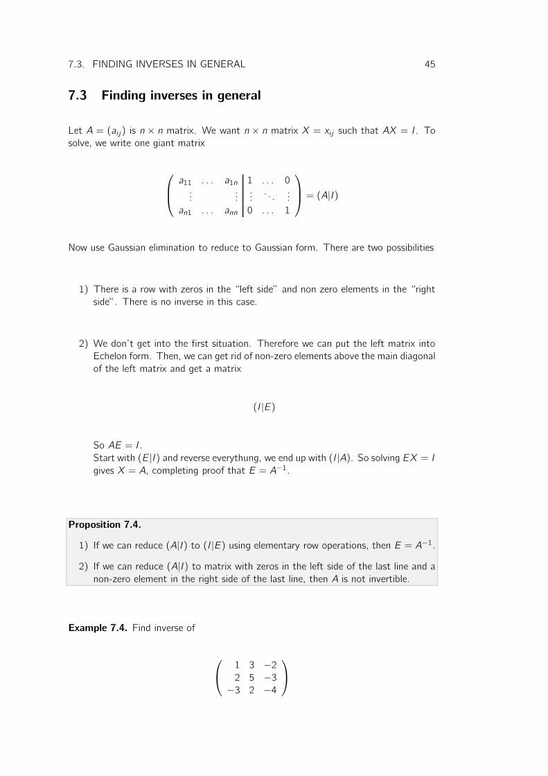
7.3 Finding inverses in general
Let A = (ai j) is n × n matrix. We want n × n matrix X = xi j such that AX = I. Tosolve, we write one giant matrix
a11 . . . a1n 1 . . . 0...
....... . .
...
an1 . . . ann 0 . . . 1
= (A|I)
Now use Gaussian elimination to reduce to Gaussian form. There are two possibilities
1) There is a row with zeros in the “left side” and non zero elements in the “right
side”. There is no inverse in this case.
2) We don’t get into the first situation. Therefore we can put the left matrix into
Echelon form. Then, we can get rid of non-zero elements above the main diagonal
of the left matrix and get a matrix
(I|E)
So AE = I.
Start with (E|I) and reverse everythung, we end up with (I|A). So solving EX = Igives X = A, completing proof that E = A−1.
Proposition 7.4.
1) If we can reduce (A|I) to (I|E) using elementary row operations, then E = A−1.
2) If we can reduce (A|I) to matrix with zeros in the left side of the last line and anon-zero element in the right side of the last line, then A is not invertible.
Example 7.4. Find inverse of
1 3 −22 5 −3−3 2 −4

46 7.3. FINDING INVERSES IN GENERAL
Augmented matrix is
1 3 −2 1 0 02 5 −3 0 1 0−3 2 −4 0 0 1
→
1 3 −2 1 0 0
0 −1 1 −2 1 00 11 −10 3 0 1
→
1 3 −2 1 0 0
0 −1 1 −2 1 0
0 0 1 −19 11 1
→
1 3 −2 1 0 0
0 1 −1 2 −11 00 0 1 −19 11 1
→
1 3 0 −37 22 20 1 0 −17 10 10 0 1 −19 11 1
→
1 0 0 14 −8 −10 1 0 −17 10 1
0 0 1 −19 11 1
Thus the inverse
14 −8 −1−17 10 1
−19 11 1
A result linking inverses, linear equations and echelon forms
Proposition 7.5. Let A be a square matrix n × n. The following four statements areequivalent
(1) A is invertible
(2) Any system Ax = b has a unique solution
(3) The system Ax = 0 has the unique solution x = 0
(4) A can be reduced to the identity In using ERO.
Proof. We prove (1)→ (2), (2)→ (3), (3)→ (4), (4)→ (1).(1)→ (2) Is done, x = A−1b
(2)→ (3) Is obvious
(3)→ (4) Needs to be proved.
(4)→ (1) Is proved earlier.�
47
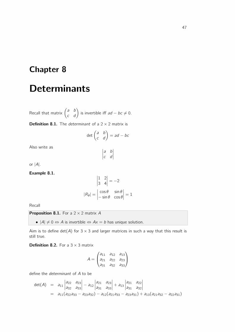
Chapter 8
Determinants
Recall that matrix
(a b
c d
)
is invertible iff ad − bc 6= 0.
Definition 8.1. The determinant of a 2× 2 matrix is
det
(a b
c d
)
= ad − bc
Also write as ∣∣∣∣
a b
c d
∣∣∣∣
or |A|.
Example 8.1. ∣∣∣∣
1 2
3 4
∣∣∣∣ = −2
|Rθ| =∣∣∣∣
cos θ sin θ
− sin θ cos θ
∣∣∣∣= 1
Recall
Proposition 8.1. For a 2× 2 matrix A
• |A| 6= 0 ⇔ A is invertible ⇔ Ax = b has unique solution.
Aim is to define det(A) for 3 × 3 and larger matrices in such a way that this result isstill true.
Definition 8.2. For a 3× 3 matrix
A =
a11 a12 a13a21 a22 a23a31 a32 a33
define the determinant of A to be
det(A) = a11
∣∣∣∣
a22 a23a32 a33
∣∣∣∣− a12
∣∣∣∣
a21 a23a31 a33
∣∣∣∣+ a13
∣∣∣∣
a21 a22a31 a32
∣∣∣∣
= a11(a22a33 − a23a32)− a12(a21a33 − a23a31) + a13(a21a32 − a22a31)
48 8.1. PROPERTIES
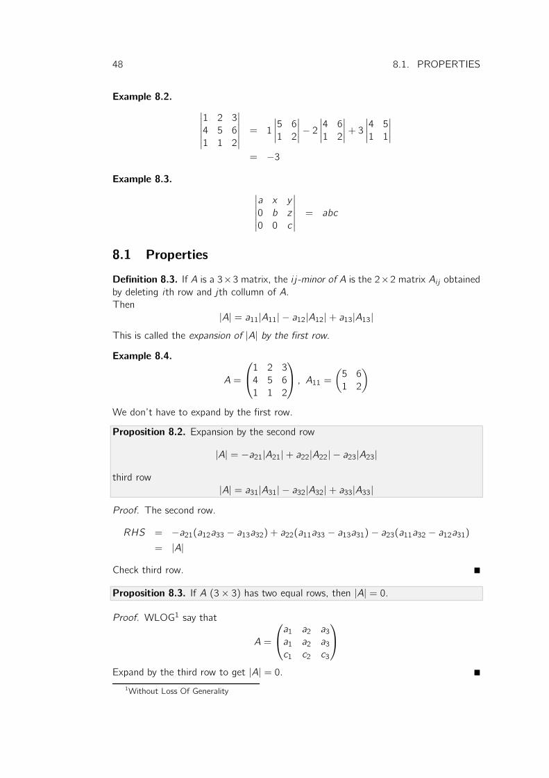
Example 8.2.
∣∣∣∣∣∣
1 2 3
4 5 6
1 1 2
∣∣∣∣∣∣
= 1
∣∣∣∣
5 6
1 2
∣∣∣∣− 2
∣∣∣∣
4 6
1 2
∣∣∣∣+ 3
∣∣∣∣
4 5
1 1
∣∣∣∣
= −3
Example 8.3.
∣∣∣∣∣∣
a x y
0 b z
0 0 c
∣∣∣∣∣∣
= abc
8.1 Properties
Definition 8.3. If A is a 3×3 matrix, the i j-minor of A is the 2×2 matrix Ai j obtainedby deleting ith row and jth collumn of A.
Then
|A| = a11|A11| − a12|A12|+ a13|A13|This is called the expansion of |A| by the first row.
Example 8.4.
A =
1 2 3
4 5 6
1 1 2
, A11 =
(5 6
1 2
)
We don’t have to expand by the first row.
Proposition 8.2. Expansion by the second row
|A| = −a21|A21|+ a22|A22| − a23|A23|
third row
|A| = a31|A31| − a32|A32|+ a33|A33|
Proof. The second row.
RHS = −a21(a12a33 − a13a32) + a22(a11a33 − a13a31)− a23(a11a32 − a12a31)= |A|
Check third row. �
Proposition 8.3. If A (3× 3) has two equal rows, then |A| = 0.
Proof. WLOG1 say that
A =
a1 a2 a3a1 a2 a3c1 c2 c3
Expand by the third row to get |A| = 0. �
1Without Loss Of Generality

8.2. EFFECTS OF ROW OPERATIONS ON DETERMINANT 49
8.2 Effects of row operations on determinant
Proposition 8.4. Let A =
r1r2r3
be 3× 3.
1) Row operation ri → ri + λrj (i 6= j). does not change |A|.
2) Swapping two rows changes |A| to −|A|.
3) Row operation ri → λri changes |A| to λ|A|
Proof.
1) Say i = 2, j = 1, so the row. op. sends
A =
a1 a2 a3b1 b2 b3c1 c2 c3
→ A′ =
a1 a2 a3b1 + λa1 b2 + λa2 b3 + λa3c1 c2 c3
Expand by the second row
|A′| = −(b1 + λa1)∣∣∣∣
a2 a3c2 c3
∣∣∣∣+ (b2 + λa2)
∣∣∣∣
a1 a3c1 c3
∣∣∣∣− (b3 + λa3)
∣∣∣∣
a1 a2c1 c2
∣∣∣∣
= |A|+ λ
∣∣∣∣∣∣
a1 a2 a3a1 a2 a3c1 c2 c3
∣∣∣∣∣∣
= |A|
2) Say we swap rows 1 and 2 to get
∣∣∣∣∣∣
b1 b2 b3a1 a2 a3c1 c2 c3
∣∣∣∣∣∣
= −a1∣∣∣∣
b2 b3c2 c3
∣∣∣∣+ . . .
3) It is obvious when we do the expansion by the row we multiply.
�
Example 8.5.
∣∣∣∣∣∣
1 2 −1−2 3 4
5 9 −4
∣∣∣∣∣∣
=
∣∣∣∣∣∣
1 2 −10 7 2
0 −1 1
∣∣∣∣∣∣
=
∣∣∣∣
7 2
−1 1
∣∣∣∣+ 0 + 0
= 9

50 8.2. EFFECTS OF ROW OPERATIONS ON DETERMINANT
Example 8.6.∣∣∣∣∣∣
1 x x2
1 y y2
1 z z2
∣∣∣∣∣∣
=
∣∣∣∣∣∣
1 x x2
0 y − x y2 − x20 z − x z2 − x2
∣∣∣∣∣∣
= (y − x)(z − x)
∣∣∣∣∣∣
1 x x2
0 1 y + x
0 1 z + x
∣∣∣∣∣∣
= (y − x)(z − x)
∣∣∣∣∣∣
1 x x2
0 1 y + x
0 0 z − y
∣∣∣∣∣∣
= (y − x)(z − x)(z − y)This is the 3× 3 Vandermande determinant.Proposition 8.5. Let A be 3 × 3 matrix, and let A′ be obtained from A by el. row.ops. Then
|A| = 0 ⇔ |A′| = 0
Proof. Doing a row op. changes |A| to |A|, -|A| or λ|A| (where λ 6= 0).�
Main result
Theorem 8.6. Let A be 3× 3 matrix. Then
|A| 6= 0⇔ A is invertible
(or the system Ax = 0 has unique solution, or A→ I3 by row ops.)Proof.
⇒ Suppose |A| 6= 0. Reduce A to echelon form A′ by row operations. By 8.5,
|A′| 6= 0. If A′ has a zero row, |A| = 0. Hence A′ =
1 · ·0 1 ·0 0 1
so can be
reduced to I. So A is invertible.
⇐ Suppose A is invertible. A can be reduced to I by row ops. Since |I| = 1, so|A| 6= 0.
�
Example 8.7. For which values of a is A invertible?
A =
1 2 5
1 3 7
1 4 a
|A| =
∣∣∣∣∣∣
1 2 5
0 1 2
0 2 a − 5
∣∣∣∣∣∣
= a − 9
So by 8.6, A is invertible iff a 6= 9.
8.3. N × N DETERMINANTS 51
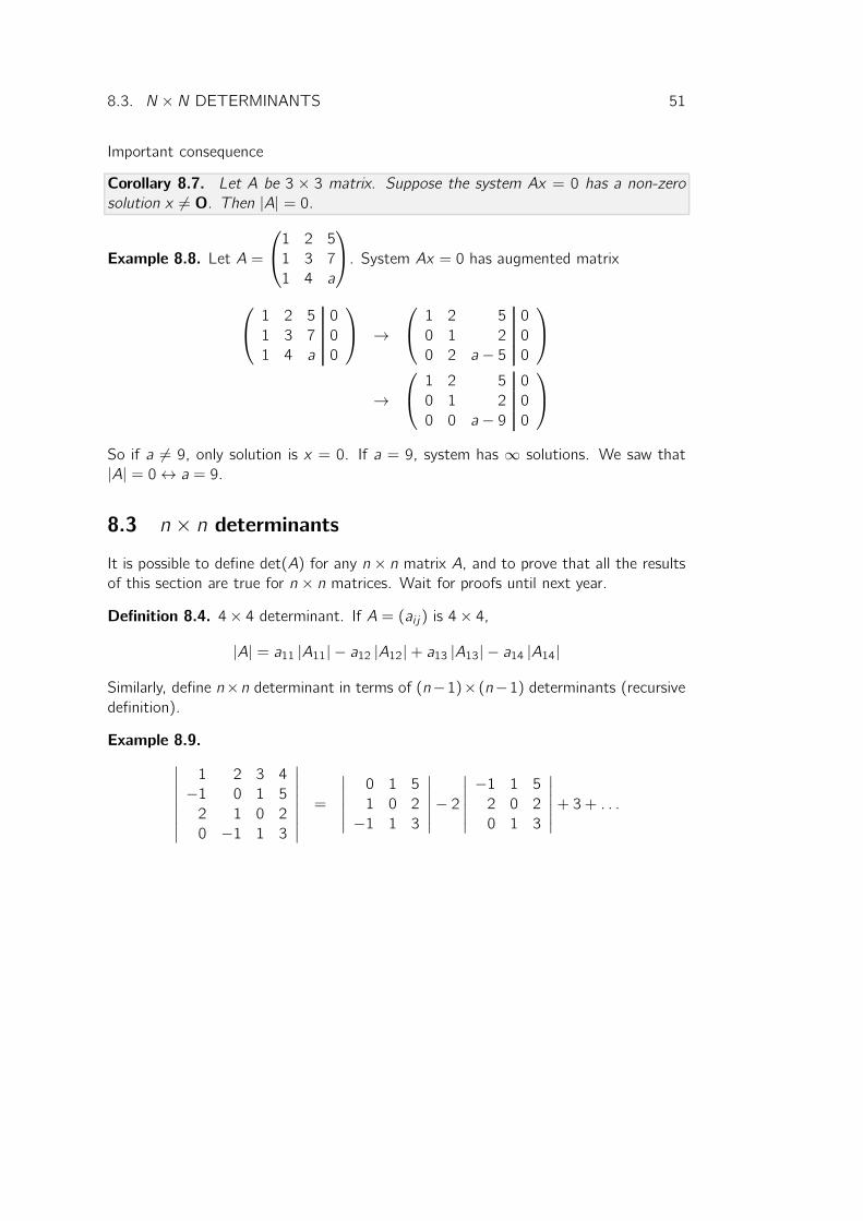
Important consequence
Corollary 8.7. Let A be 3 × 3 matrix. Suppose the system Ax = 0 has a non-zerosolution x 6= O. Then |A| = 0.
Example 8.8. Let A =
1 2 5
1 3 7
1 4 a
. System Ax = 0 has augmented matrix
1 2 5 0
1 3 7 0
1 4 a 0
→
1 2 5 0
0 1 2 0
0 2 a − 5 0
→
1 2 5 0
0 1 2 0
0 0 a − 9 0
So if a 6= 9, only solution is x = 0. If a = 9, system has ∞ solutions. We saw that|A| = 0↔ a = 9.
8.3 n × n determinantsIt is possible to define det(A) for any n × n matrix A, and to prove that all the resultsof this section are true for n × n matrices. Wait for proofs until next year.
Definition 8.4. 4× 4 determinant. If A = (ai j) is 4× 4,
|A| = a11 |A11| − a12 |A12|+ a13 |A13| − a14 |A14|
Similarly, define n×n determinant in terms of (n−1)× (n−1) determinants (recursivedefinition).
Example 8.9.
∣∣∣∣∣∣∣∣
1 2 3 4
−1 0 1 5
2 1 0 2
0 −1 1 3
∣∣∣∣∣∣∣∣
=
∣∣∣∣∣∣
0 1 5
1 0 2
−1 1 3
∣∣∣∣∣∣
− 2
∣∣∣∣∣∣
−1 1 52 0 2
0 1 3
∣∣∣∣∣∣
+ 3 + . . .

52 8.3. N × N DETERMINANTS
53
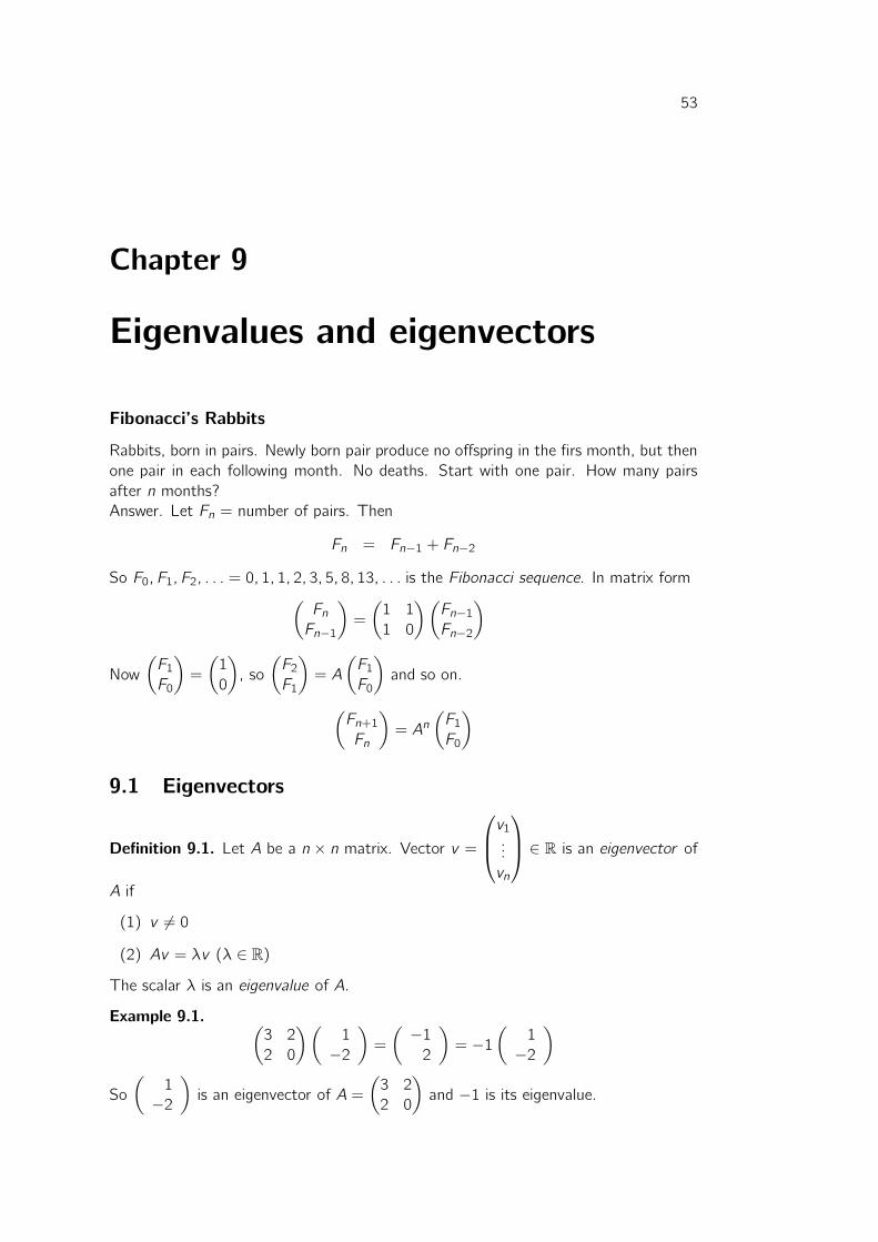
Chapter 9
Eigenvalues and eigenvectors
Fibonacci’s Rabbits
Rabbits, born in pairs. Newly born pair produce no offspring in the firs month, but then
one pair in each following month. No deaths. Start with one pair. How many pairs
after n months?
Answer. Let Fn = number of pairs. Then
Fn = Fn−1 + Fn−2
So F0, F1, F2, . . . = 0, 1, 1, 2, 3, 5, 8, 13, . . . is the Fibonacci sequence. In matrix form(FnFn−1
)
=
(1 1
1 0
)(Fn−1Fn−2
)
Now
(F1F0
)
=
(1
0
)
, so
(F2F1
)
= A
(F1F0
)
and so on.
(Fn+1Fn
)
= An(F1F0
)
9.1 Eigenvectors
Definition 9.1. Let A be a n × n matrix. Vector v =
v1...
vn
∈ R is an eigenvector of
A if
(1) v 6= 0
(2) Av = λv (λ ∈ R)
The scalar λ is an eigenvalue of A.
Example 9.1.(3 2
2 0
)(1
−2
)
=
(−12
)
= −1(1
−2
)
So
(1
−2
)
is an eigenvector of A =
(3 2
2 0
)
and −1 is its eigenvalue.

54 9.2. HOW TO FIND EIGENVECTORS AND EIGENVALUES
Example 9.2.(3 2
2 0
)(1
1
)
=
(5
2
)
6= λ(1
1
)
So
(1
1
)
is not an eigenvector of
(3 2
2 0
)
.
9.2 How to find eigenvectors and eigenvalues
Let A be a n × n matrix. Vector x is a non-zero solution of the system
Ax = λx
Example 9.3.(3 2
2 0
)(x1x2
)
= λ
(x1x2
)
We can get
(3− λ)x1 + 2x2 = 0
2x1 − λx2 = 0
So the equation is∣∣∣∣
3− λ 2
2 −λ
∣∣∣∣ = 0
λ2 − 3λ− 4 = 0
Eigenvalues are −1 and 4.For λ = −1, eigenvectors are non-zero solution of
A+ Ix = 0(4 2
2 1
)
x = 0
So eigenvectors are
(a
−2a
)
(a ∈ R, a 6= 0)For λ = 4 (
−1 2
2 −4
)
x = 0
So eigenvectors are
(2b
b
)
(b ∈ R,b 6= 0).
When does have the following equation a non-zero solution?
Ax − λx = 0
(A− λI)x = 0
Precisely when |A− λI| = 0 (by 8.6).

9.2. HOW TO FIND EIGENVECTORS AND EIGENVALUES 55
Proposition 9.1.
(1) If A is a 3×3 or 2×2, then the eigenvalues of A are the solutions λ of |A−λI| = 0.
(2) If λ is an eigenvalue, then the corresponding eigenvectors are the non-zero solu-
tions of
(A− λI)x = 0
Definition 9.2. The equation |A − λI| = 0 is the characteristic equation of A, and|A− λI| is the characteristic polynomial of A.
9.2.1 Back to Fibonacci
We had
(Fn+1Fn
)
= An(1
0
)
where A =
(1 1
1 0
)
.
Strategy
(1) Find eigenvalues λ1, λ2 and eigenvectors v1 and v2 of A. Observe
Av1 = λ1v1
Av2 = λ2v2
Then
A2v1 = A(Av1)
= A(λ1v1)
= λ1Av1
= λ21v1
Similarly
Anv1 = λn1v1
Anv2 = λn2v2
(2) Express
(1
0
)
as a combination of v1 and v2.
(1
0
)
= αv1 + βv2 (α, β ∈ R)
Then
An(1
0
)
= An(αv1 + βv2)
= αAnv1 + βAnv2
An(1
0
)
= αλn1v1 + βλn2v2 (9.1)

56 9.3. DIAGONALIZATION
Calculations
(1) Characteristic equation is |A− λI| = 0, i.e.∣∣∣∣
1− λ 1
1 −λ
∣∣∣∣= 0
i.e
λ2 − λ− 1 = 0
λ1 =1
2(1 +
√5)
λ2 =1
2(1−
√5)
Eigenvectors for λ1(1− λ 1
1 −λ
)
x = 0
So v1 =
(λ11
)
is an eigenvector.
Similarily v2 =
(λ21
)
.
(2) We now find α and β such that
(1
0
)
= α
(λ11
)
+ β
(λ21
)
α =1
λ1 − λ2β =
1
λ2 − λ1
Putting all this into (9.1)
(Fn+1Fn
)
= An(1
0
)
= αλn1v1 + βλn2v2
=1√5
(1
2
(
1−√5))n (λ1
1
)
− 1√5
(1
2
(
1−√5))n (λ2
1
)
To get formula
Fn =1√5
((1 +√5
2
)n
−(1−√5
2
)n)
9.3 Diagonalization
Want to investigate functions of matrices, e.g. An, A1n , f (A).

9.3. DIAGONALIZATION 57
Definition 9.3. An n × n matrix D is diagonal matrix if
D =
α1 O. . .
O αn
Example 9.4.(1 0
0 −2
)
It’s easy to find powers of diagonal matrices.
Proposition 9.2. Let
D =
α1 O. . .
O αn
E =
β1 O. . .
O βn
Then
DE =
α1β1 O. . .
O αnβn
and
Dk =
αk1 O. . .
O αkn
Proof. DE given by definition of matrix multiplication.
Take E = D to get D2 and repeat to get Dk . �
Aim - To relate an arbitrary square matrix A to a diagonal matrix, and exploit this to
find An, etc.
2× 2
Let A be 2×2 and suppose A has eigenvalues α1, α2 with eigenvectors v1, v2. Assumeα1 6= α2. We get
Av1 = α1v1
Av2 = α2v2
Cleverly define 2× 2 matrix P (v1, v2 are collumn vectors)
P =(v1 v2
)

58 9.3. DIAGONALIZATION
Then
AP = A(v1v2)
=(Av1 Av2
)
=(α1v1 α2v2
)
=(v1 v2
)(α1 0
0 α2
)
So if we write D =
(α1 0
0 α2
)
, we’ve shown
AP = PD (9.2)
We claim that P is invertible. For if not, then |P | = 0, which means that v1 = λv2,which is false as
Av1 = α1v1 = α1λv2
Aλv2 = λα2v2
and these are not equal as α1 6= α2.So from (9.2)
P−1AP = P−1PD = D
Summary
Proposition 9.3. Let A be 2× 2 with distinct eigenvalues α1, α2, eigenvectors v1, v2.Let
P =(v1 v2
)
Then P is invertible and
P−1AP = D =
(α1 0
0 α2
)
Note. Also true for 3× 3, . . . matrices.
Example 9.5. Let A =
(0 1
−2 3
)
.
1) Find P such that P−1AP is diagonal.
2) Find the formula An.
3) Find a 5th root of A, i. e. find B such that
B5 = A
Answer.
9.3. DIAGONALIZATION 59
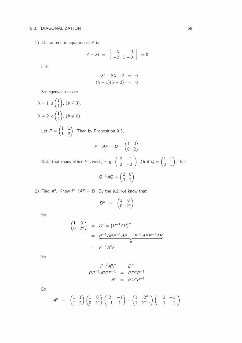
1) Characteristic equation of A is
|A− λI| =∣∣∣∣
−λ 1
−2 3− λ
∣∣∣∣ = 0
i. e.
λ2 − 3λ+ 2 = 0
(λ− 1)(λ− 2) = 0
So eigenvectors are
λ = 1 a
(1
1
)
, (a 6= 0).
λ = 2 b
(1
2
)
, (b 6= 0)
Let P =
(1 1
1 2
)
. Then by Proposition 9.3,
P−1AP = D =
(1 0
0 2
)
Note that many other P ’s work, e. g.
(2 −12 −2
)
. Or if Q =
(1 1
2 1
)
, then
Q−1AQ =
(2 0
0 1
)
2) Find An. Know P−1AP = D. By the 9.2, we know that
Dn =
(1 0
0 2n
)
So(1 0
0 2n
)
= Dn =(P−1AP
)n
= P−1APP−1AP . . . P−1APP−1AP︸ ︷︷ ︸
n
= P−1AnP
So
P−1AnP = Dn
PP−1AnPP−1 = PDnP−1
An = PDnP−1
So
An =
(1 1
1 2
)(1 0
0 2n
)(2 −1−1 1
)
=
(1 2n
1 2n+1
)(2 −1−1 1
)

60 9.3. DIAGONALIZATION
3 Find B such that B5 = A.
Well, if
C =
(1 0
0 21/5
)
Then C5 = D. So
(PCP−1)5 = PCP−1 . . . PCP−1
= PC5P−1
= PDP−1 = A
So take
B = PCP−1 =
(1 1
1 2
)(
1 0
0 215
)(2 −1−1 1
)
=
(
2− 2 15 2 15 − 12− 2 65 2 65 − 1
)
Note. Usually a matrix has many square roots, fifth roots, etc. Eg, I has infinitely
many.
Note. Similarly can calculate polynomial functions
p(A) = anAn + an−1A
n−1 + · · · + a1A+ a0I
Summary
If a square matrix A has distinct eigenvalues, then it can be diagonalized, i. e. there
exists an invertible P such that P−1AP is diagonal.
9.3.1 Repeated eigenvalues
If the characteristic polynomial of A has a repeated root λ, we call λ a repeated
eigenvalue of A.
Some A’s with the repeated eigenvalue can be diagonalised and some can’t.
Example 9.6. Let A =
(1 1
0 1
)
. Then the characteristic polynomial is
∣∣∣∣
1− λ 1
0 1− λ
∣∣∣∣= (1− λ)2
so 1 is a repeated eigenvalue. Claim A cannot be diagonalized (i.e. no invertible P
exists such that P−1AP is diagonal).
Proof. Assume there exists an invertible P such that
P−1AP = D =
(α1 0
0 α2
)

9.3. DIAGONALIZATION 61
Then
AP = PD
Writing
P =(v1 v2
)
A(v1 v2
)=
(v1 v2
)D
=(α1v1 α2v2
)
Hence Av1 = α1v1, Av2 = α2v2.
So v1, v2 are eigenvectors of A.
(0 1 0
0 0 0
)
eigenvectors are a
(1
0
)
, a 6= 0. Hence
P =
(a b
0 0
)
But this is not invertible. Contradiction. �
Point P must have evectors of A as collumns, but A does not have enough “indepen-
dent” evectors to make invertible P .
Example 9.7. Let A =
1 0 0
−1 2 0
1 −1 1
. Then the characteristic polynomial is
∣∣∣∣∣∣
1− λ 0 0
−1 2− λ 0
1 −1 1− λ
∣∣∣∣∣∣
= (1− λ)2 (2− λ)
So 1 is a repeated evalue.
Can A be diagonalized?
Let’s try.
Evectors for λ = 2
−1 0 0 0
−1 0 0 0
1 −1 −1 0
eigenvectors a
0
1
−1
, a 6= 0.
For λ = 1
0 0 0 0
−1 1 0 0
1 −1 0 0
62 9.3. DIAGONALIZATION
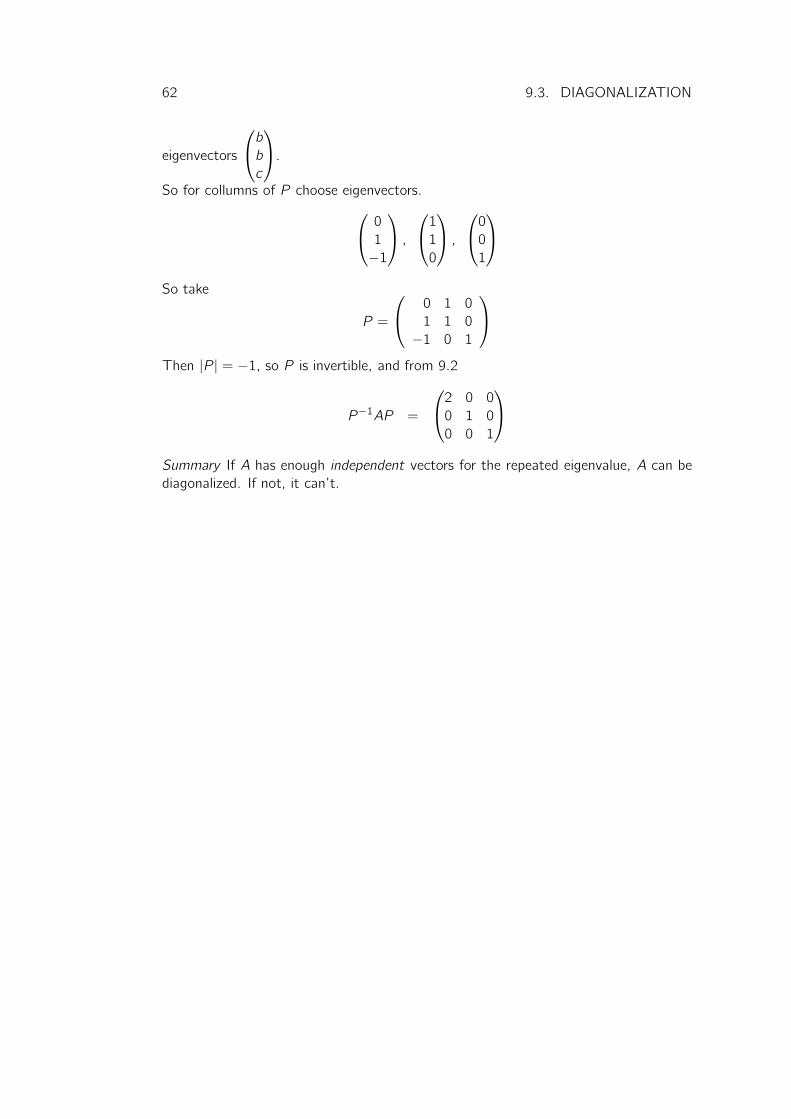
eigenvectors
b
b
c
.
So for collumns of P choose eigenvectors.
0
1
−1
,
1
1
0
,
0
0
1
So take
P =
0 1 0
1 1 0
−1 0 1
Then |P | = −1, so P is invertible, and from 9.2
P−1AP =
2 0 0
0 1 0
0 0 1
Summary If A has enough independent vectors for the repeated eigenvalue, A can be
diagonalized. If not, it can’t.

63
Chapter 10
Conics(again) and Quadrics
Recall equation of conic
ax21 + bx1x2 + cx22 + dx1 + ex2 + f = 0
We’ll write this in matrix form
(x1 x2
)(a b
2b2 c
)(x1x2
)
=(
ax1 +b2x2
b2x1 + cx2
)(x1x2
)
= ax21 + bx1x2 + cx22
So in matrix form, the equation of conic is
xTAx +(d e
)x + f = 0
where x =
(x1x2
)
, xT =(x1 x2
), A =
(a b
2b2 c
)
Digression – Transposes
Definition 10.1. If A = (ai j) is m×n, the transpose of A is them×n matrix AT = (aj i).
Example 10.1. A =
1 2
3 4
5 6
, AT =
(1 3 5
2 4 6
)
x =
(x1x2
)
, xT =(x1 x2
)
Note.
(AT )T = A
x.y =(x1 x2
)(y1y2
)
= xT y
Definition 10.2. A square matrix A is symmetric if A = AT .
Example 10.2.
(a b
2b2 c
)
is symmetric.
Proposition 10.1. Let A be m × n, B be n × p. Then
(AB)T = BTAT
64
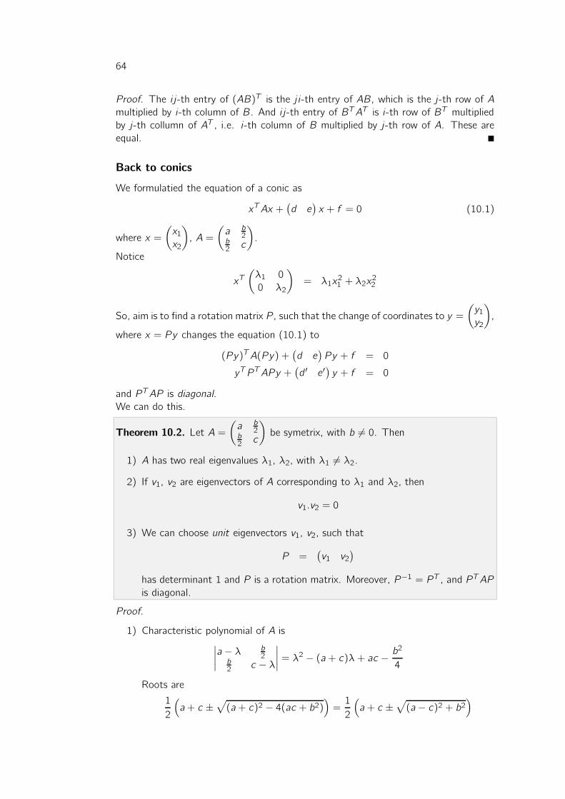
Proof. The i j-th entry of (AB)T is the j i-th entry of AB, which is the j-th row of A
multiplied by i-th column of B. And i j-th entry of BTAT is i-th row of BT multiplied
by j-th collumn of AT , i.e. i-th column of B multiplied by j-th row of A. These are
equal. �
Back to conics
We formulatied the equation of a conic as
xTAx +(d e
)x + f = 0 (10.1)
where x =
(x1x2
)
, A =
(a b
2b2 c
)
.
Notice
xT(λ1 0
0 λ2
)
= λ1x21 + λ2x
22
So, aim is to find a rotation matrix P , such that the change of coordinates to y =
(y1y2
)
,
where x = Py changes the equation (10.1) to
(Py)TA(Py) +(d e
)Py + f = 0
yTP TAPy +(d ′ e′
)y + f = 0
and P TAP is diagonal.
We can do this.
Theorem 10.2. Let A =
(a b
2b2 c
)
be symetrix, with b 6= 0. Then
1) A has two real eigenvalues λ1, λ2, with λ1 6= λ2.
2) If v1, v2 are eigenvectors of A corresponding to λ1 and λ2, then
v1.v2 = 0
3) We can choose unit eigenvectors v1, v2, such that
P =(v1 v2
)
has determinant 1 and P is a rotation matrix. Moreover, P−1 = P T , and P TAPis diagonal.
Proof.
1) Characteristic polynomial of A is∣∣∣∣
a − λ b2
b2 c − λ
∣∣∣∣ = λ
2 − (a + c)λ+ ac − b2
4
Roots are
1
2
(
a + c ±√
(a + c)2 − 4(ac + b2))
=1
2
(
a + c ±√
(a − c)2 + b2)

10.1. REDUCTION OF CONICS 65
Since b 6= 0, (a − c)2 + b2 > 0, so the roots are real and distinct. Call them λ1and λ2.
2) Let
Av1 = λ1v1
Av2 = λ2v2
Consider
vT1 Av2
(a) This is vT1 (λ2v2) = λ2vT1 v2.
(b) It is also (because A is simetric, i.e. A = AT )
(AT v1)T v2 = (Av1)
T v2 = λ1vT1 v2
So
λ2vT1 v2 = λ1v
T1 v2
As λ1 6= λ2, this forces vT1 v2 = 0, i.e. v1.v2 = 0.
3) Choose unit v1, v2 (see picture). Then
v1 =
(cos θ
sin θ
)
v2 =
(− sin θcos θ
)
So
P =(v1 v2
)
=
(cos θ − sin θsin θ cos θ
)
= Rθ
Finally, by 9.3 ,
P TAP = P−1AP =
(λ1 0
0 λ2
)
�
10.1 Reduction of conics
Start with equation (10.1).
1) Find the evalues and evectors of A
2) Find unit eigenvectors v1, v2, such that P =(v1v2
)has determinant 1, so is a
rotation matrix.
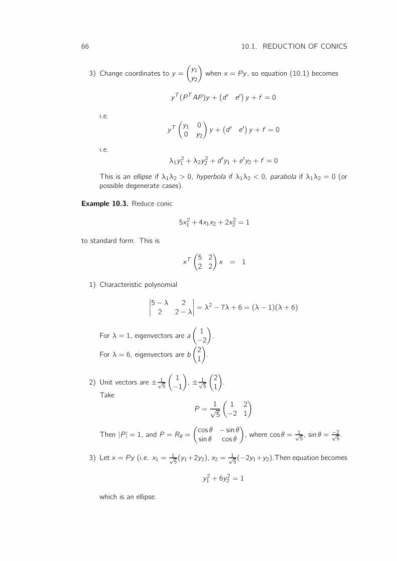
66 10.1. REDUCTION OF CONICS
3) Change coordinates to y =
(y1y2
)
when x = Py , so equation (10.1) becomes
yT (P TAP )y +(d ′ e′
)y + f = 0
i.e.
yT(y1 0
0 y2
)
y +(d ′ e′
)y + f = 0
i.e.
λ1y21 + λ2y
22 + d
′y1 + e′y2 + f = 0
This is an ellipse if λ1λ2 > 0, hyperbola if λ1λ2 < 0, parabola if λ1λ2 = 0 (or
possible degenerate cases).
Example 10.3. Reduce conic
5x21 + 4x1x2 + 2x22 = 1
to standard form. This is
xT(5 2
2 2
)
x = 1
1) Characteristic polynomial
∣∣∣∣
5− λ 2
2 2− λ
∣∣∣∣ = λ
2 − 7λ+ 6 = (λ− 1)(λ+ 6)
For λ = 1, eigenvectors are a
(1
−2
)
.
For λ = 6, eigenvectors are b
(2
1
)
.
2) Unit vectors are ± 1√5
(1
−1
)
, ± 1√5
(2
1
)
.
Take
P =1√5
(1 2
−2 1
)
Then |P | = 1, and P = Rθ =(cos θ − sin θsin θ cos θ
)
, where cos θ = 1√5, sin θ = −2√
5.
3) Let x = Py (i.e. x1 =1√5(y1+2y2), x2 =
1√5(−2y1+y2).Then equation becomes
y21 + 6y22 = 1
which is an ellipse.

10.2. QUADRIC SURFACES 67
10.1.1 Orthogonal matrices
Recall, rotation matrix satisfies
RTθ = Rθ
So does a reflection matrix(cos θ sin θ
sin θ − cos θ
)
Definition 10.3. A square matrix P is an orthogonal matrix if P T = P−1, i. e.PP T = I.
The key property:
Proposition 10.3. Orthogonal matrices preserve lengths, i. e.
‖Pv‖ = ‖v‖
Proof.
‖Pv‖2 = (Pv).(Pv)
= (Pv)T (Pv)
= vTP TPv
= vT Iv
= ‖v‖2
�
10.2 Quadric surfaces
Definition 10.4. A quadric surface is a surface in R3 defined by a quadratic equation
ax21 + bx22 + cx
23 + dx1x2 + ex1x3 + f x2x3 + gx1 + hx2 + jx3 + k = 0 (10.2)
Standard examples
1) Ellipsoidx21a2+x22b2+x23c2= 1
2) Hyperboloid of 1 sheetx21a2+x22b2− x
23
c2= 1
3) Hyperboloid of 2 sheetsx21a2+x22b2− x
23
c2= −1
4) Elliptic conex21a2+x22b2− x
23
c2= 0

68 10.2. QUADRIC SURFACES
5) Elliptic parabloid
x3 =x21a2+x22b2
6) Hyperbolic parabloid
x3 =x21a2− x
22
b2
Some degenerate cases
7) Elliptic cylinder
x21a2+x22b2= 1
8) Parabolic cylinder
x21 − ax2 = 0
Aim is to find a rotation and translation, which reduces (10.2) to one of the standard
examples. Here is the procedure.
1. Write (10.2) in matrix form
xTAx +(g h j
)x + k = 0
where
x =
x1x2x3
A =
a d2
e2
22 b f
2e2
f2 c
Notice that A is symmetric.
2. Find the eigenvalues λ1, λ2, λ3 of A (theory – these are real). Find corresponding
unit eigenvectors v1, v2, v3 which are perpendicular to each other (theory – this
can be done). Choose a directions for the vi so that the matrix
P =(v1 v2 v3
)
has determinant 1.
Then, P is a rotation matrix, and P−1 = P T . Then
P−1AP = P TAP
=
λ1 0 0
0 λ2 0
0 0 λ3

10.2. QUADRIC SURFACES 69
3. Change coordinates to y =
y1y2y3
, where x = Py . Then (??) reduces to
yT (P TAP )y +(g h j
)Py + k = 0
i. e.
λ1y21 + λ2y
22 + λ3y
23 + g
′y1 + h′y2 + j
′y3 + k = 0
Finally, complete the square to find translation reducing to a standard equation.
Note. All the assumed bits of theory will be covered in Algebra II next year.
Example 10.4. Reduce the quadric
2x1x2 + 2x1x3 − x2 − 1 = 0
to standard form.
Answer.
1. Equation is
xT
0 1 1
1 0 0
1 0 0
x = x2 + 1
2. Characteristic polynomial is
∣∣∣∣∣∣
−λ 1 1
1 −λ 0
1 0 −λ
∣∣∣∣∣∣
= −λ(λ2 − 2)
We get λ equal to 0,√2, −√2.
Eigenvectors.
For λ = 0 a
0
1
01
, unit eigenvectors ± 1√2
0
1
1
For λ =√2 b
√2
1
1
, unit eigenvectors ±
1√21212
For λ = −√2 b
−√2
1
1
, unit eigenvectors ±
− 1√21212
Let
P =
0 1√2− 1√
2
− 1√2
12
12
1√2
12
12

70 10.3. LINEAR GEOMETRY IN 3 DIMENSIONS
Then |P | = 1 and P is a rotation.Change of coordinates x = Py changes equation to
√2y22 −
√2y23 = −
1√2y1 +
1
2y2 +
1
2y3 + 1
Finally, complete the square
√2(y2 − α)2 −
√2(y3 − β)2 = −
1√2(y1 − γ)
This is a hyperbolic paraboloid.
10.3 Linear Geometry in 3 dimensions
Definition 10.5. For two vectors x = (x1, x2, x3), y = (y1, y2, y3) in R3, define
• x + y = (x1 + y1, x2 + y2, x3 + y3)
• λx = (λx1, λx2, λx3), λ ∈ R
• length of x , denoted ‖x‖ =√
x21 + x22 + x
23
• dot product x.y = x1y1 + x2y2 + x3y3 (note that x.x = ‖x‖2)
Proposition 10.4. For x, y ∈ R3
x.y = ‖x‖‖y‖ cos θ
Proof.
‖y − x‖2 = ‖x‖2 + ‖y‖2 − 2‖x‖‖y‖ cos θ2‖x‖‖y‖ cos θ = x.x + y .y − (y − x)(y − x)
= 2x.y
�
10.4 Geometry of planes
Fact – there is a unique plane through any 3 points in R3 provided thay aren’t colinear.
We want to describe planes in terms of vectors and equations.
A plane Π in R3 is specified by
1) a point A on the plane
2) a vector n normal to the plane
Then x ∈ Π⇔ (x − a).n = n ⇔ x.n = a.n.
Proposition 10.5. If there are points A,B, C ∈ R3 that are not collinear, there existsa unique plane Π through A,B, C.

10.4. GEOMETRY OF PLANES 71
Proof. Because both A− B and B − C are both in the plane
n.(a − b) = 0
n.(c − a) = 0
i.e.
r1n1 + r2n2 + r3n3 = 0
s1n1 + s2n2 + s3n3 = 0
where (r1, r2, r3) = a − b, (s1, s2, s3) = c − a.We want to show that all solutions are {λn | λ ∈ R}. Because A, B, C are not colinear,r and s are not parallel. �
How to find dist(P,Π)?
Find foot of perpendicular, Q and arbitrary A in the plane.
dist(P,Q) = ‖a − p‖ cos θ
But
(a − p).n = ‖a − p‖‖n‖ cos θ
dist(P,Q) =(a − p).n‖n‖

72 10.4. GEOMETRY OF PLANES
Notes
![Bio Soil Interactions Engineering Workshop1].pdf · Bio‐Soil Interactions & Engineering Workshop ... Notes. Notes. Notes. Notes. Notes. Notes. ... Electrokinetic and Electrolytic](https://img.dokumen.tips/doc/110x75/5e7be480f39bf41290742405/bio-soil-interactions-engineering-workshop-1pdf-bioasoil-interactions-.jpg)