Lower Bounds for Multi-Echelon Stochastic Inventory Systems

Lower Bounds for Multi-echelon Stochastic

Inventory Systems

Fangruo Chen * Yu-Sheng Zheng Graduate School of Business, Columbia University, New York, New York 10027

Operations and Information Management Department, The Wharton School, University of Pennsylvania, Philadelphia, Pennsylvania 19104

e establish lower bounds on the minimum costs of managing certain production- distribution networks with setup costs at all stages and stochastic demands. These net-

works include serial, assembly, and one-warehouse multi-retailer systems. We obtain the bounds through novel cost-allocation schemes. We evaluate the bounds' performance for one-warehouse multi-retailer systems by comparing them with simple, heuristic policies. The bounds are quite tight for systems with a small number of retailers. We also present simplified proofs of known optimality results for serial and assembly systems. (Stationary Analysis; Cost Allocation; Economies of Scale; Multi-stage Production Systems; Distri- bution Networks; Replenishment Strategies)

. Introduction his paper establishes lower bounds on the minimum )sts of managing certain production-distribution net- rorks with setup costs at all stages and stochastic de- iands. These networks include serial, assembly, and ne-warehouse multi-retailer systems. This study was iotivated by our effort to identify cost-effective control olicies for these systems. It is well known that optimal zntrol of these systems is difficult due to the presence f setup costs, especially at downstream stages (Clark nd Scarf 1962). As a result, heuristic control policies ecome attractive. Tight lower bounds on the minimum )sts are necessary to evaluate the effectiveness of heu- stic policies. We obtain lower bounds through novel cost-

[location schemes. Cost allocation has been successfully pplied to obtain lower bounds for several related multi- :age systems by Roundy (1985, 1986), Atkins and Iyo- un (1987) and Zheng (1987), among others. (See At- ins 1990 for a review on cost allocation as well as other )wer-bounding methodologies.) For more general sys- jms, new lower bounds can be created by combining zst allocation with "physical decomposition." In par- cular, imagine that the product consists of a number

of fictitious components. Each component is supplied/ produced through a subsystem-a part of the original system-and is allocated part of the costs. By assuming that the components can be replenished and sold sep- arately (i.e., physical decomposition), the original system decomposes to a number of independent systems, one for each component. The sum of the minimum costs of these independent systems is a lower bound on the minimum cost of the original system.

The virtue of the cost - allocation, physical- decomposition framework is that it provides freedom in creating fictitious components and in allocating costs. By allocating one-period expected holding and backorder cost functions (hereafter referred to as loss functions), we re-derive and generalize the so-called "induced-penalty bounds" for serial systems (Clark and Scarf 1962 and Atkins and De 1992) and for one- warehouse multi-retailer systems (Rosling 1977). On the other hand, by allocating cost rates, we generate a new class of bounds, called "parameter-allocation bounds." These bounds are derived for both periodic- review and continuous-review, stationary systems op- erating over an infinite horizon.

Our lower-bounding framework depends upon sev-

0025-1909/94/401 1/1426$01 .25 126 MANAGEMENT SCIENCE/VOL. 40, No. 11, November 1994 Copyright ? 1994, The Institute of Management Sciences

CHEN AND ZHENG Lower Bounids for Multi-echeloni Stochastic Iniventony Systems

eral key results in the multi-echelon inventory literature. These include the optimal policies for the periodic- review, serial system of Clark and Scarf (1960) and Federgruen and Zipkin (1984b) and the periodic- review, assembly system of Rosling (1989), and the lower bound for the one-warehouse multi-retailer system of Federgruen and Zipkin (1984a, b, c). In this paper, we provide a simpler proof for the above optimality results (for serial and assembly systems). We first establish (induced-penalty) lower bounds on the minimum costs of these systems, and then show that these lower bounds can actually be achieved by feasible policies. Therefore the feasible policies are optimal and the lower bounds are the minimum costs. This method also leads to parallel optimality results for the continuous-review counterparts of the above systems.

We have conducted a numerical test of the bounds' performance by comparing them with simple, heuristic policies in one-warehouse multi-retailer systems. The results indicate that the bounds are tight for systems with a small number of retailers.

The paper is organized as follows. Sections 2-4 focus on periodic-review systems. In ?2, we define the systems to be considered and review related known results. In ?3, we present the new optimality proofs for serial and assembly systems. In ?4, we establish lower bounds for serial, assembly, and one-warehouse multi-retailer systems with setup costs at all stages. Section 5 describes briefly how the optimality results and lower bounds can be extended to continuous-review systems. In ?6, we report the numerical study. Section 7 contains concluding remarks.

2. The Models In this section, we describe the models to be studied, review relevant known results, and define general no- tation. Consider serial, assembly, and one-warehouse multi-retailer systems with stochastic demand. (Since one-warehouse multi-retailer systems are the only distribution systems considered in this paper, they will be referred to as distribution systems in the sequel.) Here we concentrate on periodic-review systems. The following assumptions are common to all the systems:

* Each system produces or distributes a single final product through multiple stages. A stage can be a dis- tinctive location in distribution systems or a buffer for

a particular intermediate item in production systems. The stage(s) that receives stock from an outside supplier is called the "highest" stage. The stage(s) where customer demand arises is called the "lowest" stage.

* The transportation (or production) leadtime at stage i is a constant of Li periods, i.e., a batch released to stage i at the beginning of period t will be received at the beginning of period t + Li.

* Customer demands at different periods are independent and identically distributed. F denotes the cu- mulative distribution function (cdf) of one-period demand. If customer demand arises at more than one stage, F denotes the joint cdf. Demand is discrete.

* Replenishment decisions are centralized and based on system-wide inventory information, which is avail- able and free. The objective is to minimize long-run average system-wide costs.

* A fixed setup cost Ki is incurred for each batch released to stage i.

* The echelon holding cost at stage i is hi per unit* period. It is more expensive to hold inventory at a lower stage than at an upper stage, i.e., hi 2 0.

* Unsatisfied customer demand is fully backlogged at the lowest stage with penalty cost p per unit * period. For systems where demand occurs at several stages, the penalty cost is pi at stage i.

Serial systems. The system consists of N stages ar- ranged in series with stage 1 receiving stock from stage 2, 2 from 3, etc., and stage N from an outside supplier with infinite stock. Customer demand occurs only at stage 1. Denote the system by "Series (N)." When only stage N has a setup cost K, i.e., KN = K and Ki = 0 for 1 ? i ? N - 1, denote the system by "Series(N, K)."

Assembly systems. The system produces a final product through a tree structure, denoted by ., with N stages. More specifically, each stage has exactly one successor stage, except for the lowest stage (the root of the tree) where customer demand arises. The stages without any predecessor stage (the leaves of the tree) are replenished by outside suppliers with infinite stock. Without loss of generality, we assume that exactly one unit of each intermediate item is used to produce its immediate successor item. We will refer to the above assembly system as "Assembly ( s)." Let S ( i) be the set consisting of stage i and all its successor stages. Define Mi as the total leadtime at stage i, i.e., Mi =j E&S(i) Lj.

MANAGEMENT SCIENCE/VOl. 40, No. 11, November 1994 1427

CHEN AND ZHENG Lower Bounids for Multi-echeloni Stochastic Inivenitory Systems

The stages are numbered such that Mi is nondecreasing in i. (Thus stage 1 is the lowest stage.) When only stage N, the stage with the longest total leadtime, has a setup cost K, the above system will be referred to as "Assem- bly(., K)."

Distribution systems. The system has one warehouse and N retailers. The warehouse (stage 0) receives stock from an outside supplier with infinite stock and replenishes the retailers (stages 1, . . . , N). Customer demands occur only at the retailers. The above system will be denoted by "Distribution(N)," or by "Distri- bution(N, K)" when only the warehouse has a setup cost K.

We proceed to briefly review the existing results on Series(N, K), Assembly(&, K), and Distribution(N, K), which are the building blocks of our lower bounds.

Note that Series(1, K) or Series(1) is the extensively studied single-location system. For this system, it is well known that (s, S) policies are optimal. (See Scarf 1960 and Iglehardt 1963 for the original proof, and Zheng 1991 for a simple proof.) Under an (s, S) policy, an order is placed to increase the inventory position (= inventory on hand + outstanding orders - backorders) to S whenever it drops to or below s. The minimum cost of the system is therefore the cost associated with the optimal (s, S) policy. For a simple and efficient algorithm to compute optimal (s, S) policies, see Zheng and Federgruen (1991).

In their seminal paper, Clark and Scarf (1960) characterized the optimal policies for the finite-horizon ver- sion of Series(N, K). Their result was extended by Fed- ergruen and Zipkin (1984b) to infinite-horizon systems. An optimal policy for Series(N, K) uses an echelon stock (s, S) policy at stage N and an echelon stock order-up- to policy at each downstream stage. We denote the minimum cost of Series(N, K) by a function of the system parameters, CN(K, h, p, L, F), where h = { Nh }N and L = { L, } . A new derivation of the optimal policy and its minimum cost will be provided in ?3.

For Assembly(., 0), Rosling (1989) characterized the optimal policies by showing that the system is equivalent to a serial system by introducing the notion of total leadtimes. Section 3 provides a simple proof that this equivalence holds for Assembly ( 1, K). Denote the minimum cost of Assembly(1, K) by C' (K, h, p, L, F), where h = {hi }N and L = {Li }N

Optimal policies for Distribution(N, K) are unknown. The difficulty is due to possible stock imbalance among different retailers (Eppen and Schrage 1981, Zipkin 1984). However, Federgruen and Zipkin (1984a, b, c) provided a lower bound on the minimum cost of the system by allowing a free inventory (position) rebalance among the retailers. Under such a relaxation, the original system reduces to a single-location system whose minimum cost can be easily computed. This minimum cost is a lower bound on the minimum cost of the original system. Denote this lower bound by Cd (K, h, p, L, F), where h = {hi }o, P = {pi }N and L = {Li }. (Notice that h and L are being used to represent different vectors in different contexts.)

We proceed to define key state variables. Echelon inventory level at stage i is the inventory on hand at stage i plus inventories at or in transit to all its successor stages minus total customer backorder at stage i and its successor stages. Echelon inventory position at stage i is the sum of echelon inventory level at stage i and the inventories in transit to stage i. Assume that the activities in a period happen in the following sequence: (a) at the beginning of the period, replenishment batches are released and received; (b) during the period, customer demand occurs; and (c) at the end of the period, holding and backorder costs are assessed based on the ending inventory and backorder levels. Fix a period t. Let IL (t) and IPi (t) be the (beginning) echelon inventory level and the echelon inventory position at stage i after replenishment batches are released and received but before demand occurs. At the end of period t (after demand), let

Ii (t) = echelon inventory at stage i = inventory on hand at stage i plus inventories

at or in transit to all its successor stages Bi (t) = customer backorder level at stage i, defined

only if customer demand arises at stage i; use B(t) if customer demand arises only at one stage

ILi (t) = (ending) echelon inventory level at stage i For t1 c t2, we use [t1, t2] to denote the time interval

of periods t1, . . . , t2 . Similarly, we use [ t1, t2) to denote the time interval of periods t1, . . ., t2-1. For Series (N) and Assembly (1s), let D[ t1, t2] and D[t1, t2) be the total customer demand in [t1, t2] and [t1, t2) respectively for any t1 ? t2 with D[t, t) 0. For Distribution(N), let

1428 MANAGEMENT SCIENCE/Vol. 40, No. 11, November 1994

CHEN AND ZHENG Lower Bounds for Multi-echelon Stochastic Inventony Systems

Di [ ti, t2] and D [tl, t2) be the total customer demand at retailer i, 1 ? i ? N, in [ ti, t2] and [ ti, t2) respectively for any t, ? t2 with Di [ t, t) 0. Let Do[ tl, t2] = 1 Di[tj, t2] and Do[ tl, t2) = 1 Di[t1, t2)

3. Optimality Proofs In this section, we rederive the optimality results for Series(N, K) and Assembly(., K) by first establishing lower bounds on the minimum costs of the systems and then showing that the bounds can be reached by feasible policies.

3.1. Series(N, K) Consider any feasible policy for Series(N, K). The total holding and backorder cost incurred at period t is

N

E hi (t) + pB(t).

Since ILi(t) = Ii(t) - B(t), the above expression can be rewritten as

N

hILi(t) + (p + H1)B(t) i=l

where H1 NI= hi, the installation holding cost at stage 1. For convenience, we charge the following cost to period t - MN

N

E hiILi(t - Mi1) + (p + Hi)B(t) (1) i=l

where Mo =0 and Mi = E 41 Lj for i = 1, .. . , N. Notice that Mi is the total leadtime at stage i. This cost accounting scheme only shifts costs across time periods. Therefore, it does not affect the long-run average holding and backorder costs. The accounting scheme has the following intuitive interpretation: Since ILi (t -Mi-1) = IPi(t - Mi) - D[t - Mi, t -Mi- ], we see that ILi(t - Mi1) is statistically determined by IPi (t - Mi). Moreover, by definition, IPi (t -Mi ) is constrained by the beginning echelon inventory level at stage i + 1, i.e. IPi (t - Mi ) ? IL - 1(t - Mi ), with the difference being the on-hand inventory at stage i + 1. But IL i-+ (t - Mi) is, in turn, statistically determined by Pi+l (t - Mi+l): IL -1 (t - Mi) = Pi+l (t - Mi+) - D[ t

- Mi+?, t - Mi). A simple induction shows that IPN(t

- MN) determines, directly or indirectly, ILi (t -Mi-)

for i = 1, . . . , N. Therefore it is meaningful to charge the holding and backorder cost in (1) to period t - MN

when the decision on IPN (t - MN) is made. For sim- plicity, write IPi for IPi (t - Mi), ILi for ILi (t -Mi-1), IL7 for IL (t - Mi1), and B for B(t). Consequently, the total holding and backorder cost charged to period t - MN is

N

hiILi + (P + H1)B (2)

Next, we identify a lower bound on the expected value of (2). Define

Gl(y) = E[h1(y - D[t - Ml, t])

+ (p + Hl)(y - D[t - Ml, t])-].

Notice that G1 (*) is convex. Let Y1 be a minimum point of Gl(*) and Cl G1(Y1). Define

Cl if y ? Y

GG (y) otherwise

G l2(y) = Gl(y) - Gl(y)

and

G2(y) = E[h2(y - D[t -M2, t - M1])

+ G2(y - D[t - M2, t -Ml))]

Note that both G (*) and G2(*) are convex. The above definitions can be extended inductively. In particular, suppose that Gi ( * ), 2 ? i < N, are defined and convex. Let Yi be the minimum point of Gi (*) and Ci = Gi (Yi). Define

Ci if y ? Yi

G(YJl=Gi (y) otherwise

G'+ 1(y) = Gi (y) -G (y)

and

Gi+l(y) = E[hi+l(y - D[t - Mi+,, t - M])

+ G+l (y - D[t - Mi+?, t Mi- .

By induction, it is easy to see that the Gi (* )'s are all convex. (The above functions were introduced by Ros- ling 1989 under a slightly different form.) Now consider a single-stage system with setup cost K, loss function


CHEN AND ZHENG Lower Bounids for Multi-echeloni Stochastic Inivenitory Systenms

GN( ), and the demand process of the original system. We know that (s, S) policies are optimal. Let (SN, SN)

be the optimal (s, S) policy and CN the minimum cost of the single-stage system. (The above definitions will also be used in discussing assembly systems.)

LEMMA 1. For Series (N, K), we have E[ N=l hiIL + (p + H1)B] 2 E[ IN-1 G'(IPi) + GN(IPN)].

PROOF. Since IL1 = IP1 - D[t - M1, t] and B (IL1)-, from the definition of G1(*) we have

E[h1IL1 + (p + H1)B] = EG1(IP1).

Since IP1 ? IL - and G 2( () is nonincreasing, we have G1(IPl) = GI(IPl) + G2(IP1) ? G (IPl) + G2(ILy). Therefore

E[, hiILi + (p + H1)B]

? E[G1(IP1) + h2IL2+ G 2G(IL )]

Notice that G 2(IL- ) corresponds to the induced-penalty cost in Clark and Scarf (1960). It represents the expected holding and backorder cost increment at stage 1 when stage 2's on-hand stock is insufficient to bring stage l's inventory position up to Y1, i.e. IL F < Y1. Charging this induced-penalty cost to stage 2, we have

E[h2IL2 + G2(IL-)] = E[h2(IP2 - D[t - M2, t - M1])

+ G1(IP2 - D[t - M2, t -M))]

= EG2(1P2)

Therefore,

Ep I hiILi + (p + Hi)B] ? E[G}(IP1) + G2(IP2)].

The lemma is now true for N = 2. A simple induction verifies the lemma for any value of N. O

LEMMA 2. zI=, Ci is a lower bound on the minimum long-run average cost of Series(N, K).

PROOF. Recall that Ci is the minimum value of Gi (*) for i < N. Thus, it follows from Lemma 1 that

- N ( N-1

EE hi ILi + (p + Hi ) B | Ci + EGN (IPN)-

In other words, given IPN = y, the expected systemwide holding and backorder costs charged to period t - MN

under any policy are bounded below by i =1 C, + GN(Y). By substituting the latter for the former, the original system reduces to a single-stage system with setup cost K and loss function E iN-1 Ci + GN(Y). Since LiN=1 C, is constant, the optimal policy of this single- stage system is the (SN, SN) policy with minimum cost

i=1 Ci. Clearly, this minimum cost is a lower bound on the minimum cost of Series(N, K). O

We next show that the above lower bound can be achieved by a feasible policy. Consider the following feasible policy for Series(N, K). Stage N uses the echelon stock (SN, SN) policy: if the echelon inventory position at stage N falls to or below SN then order up to SN; and stage i, i = 1, . . ., N - 1, uses an echelon stock order- up-to Yi policy: if the echelon inventory position at stage i is below Yi then order up to Yi. This is indeed the optimal policy characterized by Clark and Scarf (1960) and Federgruen and Zipkin (1984b). To prove its optimality, it suffices to show that it actually achieves the lower bound E I=1 Ci.

THEOREM 1. For Series(N, K), the optimal policy uses the echelon stock (SN, SN) policy at stage N and the echelon stock order-up-to Yi policy at stage i, i = 1, . .. , N - 1, with minimum cost Cs(K, h, p, L, F) = , Ci.

PROOF. Suppose that the above policy is in place for Series(N, K). All we need to show is that, given IPN = y, the expected system-wide holding and backorder costs charged to period t - MN are exactly equal to

i= C + GN(Y)- Take any i < N. Notice that IPi ? IL - 1. Since stage

orders up to Yi, we have IPi = min{Yi, IL - 1 }. Thus G (IPj) = Ci. Therefore it only remains to show that the inequality in Lemma 1 is an equality. To see this, simply notice that G'+1(IPi) = G'+1(IL - 1) since if IP,

Yi then IL -I1 ? Yi and thus G'+1(IPi) = G'+1(IL -71) = 0. D

We proceed to interpret the above lower bound and optimality proof under a cost-allocation framework. For ease of presentation, we only consider Series(2, K). Imagine that the end product (at stage 1) consists of two components, 1 and 2. The subsystem that supplies component 2 is exactly the same as the original system. But component 1 is supplied through a truncated sys-

1430 MANAGEMENT SCIENCE/VOL. 40, No. 11, November 1994

CHEN AND ZHENG Lower Bounds for Multi-echelon Stochastic Inventory Systems

tem: it is directly sourced from an outside vendor with ample supply. The delivery leadtime from the vendor to stage 1 is L1, the same as the transportation time from stage 2 to stage 1. In the original system, replenishment is "coordinated" between the two components: each unit of component 2 leaving stage 2 is matched by a unit of component 1 leaving the outside vendor. After arriving at stage 1, these components are sold in packages. Since component 2 is the only item at stage 2, it bears the setup cost K at stage 2 and the stage-2 echelon holding cost with rate h2. The loss function at stage 1, G1 (*), is shared by the two components: G I (* ) by component 1 and the remaining, G1(*), by component 2. (The systems of the components are depicted in Figure 1.) Notice that the above cost allocation fully recovers the total costs of the original system.

Now relax the above coordination constraint by assuming that the components can be replenished and sold independently of each other. Under this relaxation, the original system decomposes to two independent systems, one for each component. The sum of the minimum costs of the components is a lower bound on the minimum cost of the original system.

The system of component 1 is a single-stage system with loss function G (.) and no setup cost. Thus its minimum cost is C1 = G 1(Y1), which can be reached by any policy that keeps the inventory position of component 1, IP1, at or below Y1. Now consider the system of component 2. Notice that the loss function at stage

Figure 1 Decomposition of Series (2, K)

System of System of Series(2,K) Component 1 Component 2

+

1 1

YI Y1 Y1

1, G 2(IPF), is a nonincreasing function of IP1. Since no setup cost is incurred for shipping stock from stage 2 to stage 1, there is no incentive to hold inventory at stage 2. Therefore an optimal policy would keep IP1 = IL - and the system collapses to a single-stage system. Since IL2 = IP2 - D[t - M2, t - M1] and IL-2 =I2 - D[t - M2, t - M1), the total holding and backorder cost of component 2 can be expressed as a loss function of its echelon inventory position at stage 2, IP2:

E[h2IL2 + G 2(IPl)] = E[h2IL2 + G2(IL2j)]

= E[h2(IP2 - D[t - M2, t -M1])

+ GW(IP2 - D[t - M2, t -M))]

= EG2(1P2).

Therefore the resulting single-stage system has loss function G2( ( ) and setup cost K. Since G2 ( ) is convex, the (s2, S2) policy is optimal with minimum cost C2. Thus, C1 + C2 is a (induced-penalty) lower bound on the minimum cost of Series(2, K).

To show Theorem 1, recall that the only relaxation used to generate the lower bound is that the components can be replenished and sold independently of each other. Therefore, it suffices to show that there exist optimal policies for the component systems such that the components arriving at stage 1 are exactly matched. First consider component 2. The optimal policy for component 2 is to use the echelon stock (s2, S2) policy at stage 2 and ship all to stage 1 (i.e., ship up to IL2-). However, since G 2(y) is flat for y 2 Y1, the policy remains optimal if stage 2 ships up to min{Y1, IL - }. Now consider component 1. Since G (y) is flat for y < Y1, any policy that does not raise the inventory position of component 1 to above Y1 is optimal. One such policy is to ship up to min{ Y1, IL - }. Observe that under the above optimal policies in the component systems, the components arriving at stage 1 are exactly matched. This completes the proof for the theorem. The above cost-allocation approach will be used in ?4 to derive a similar bound for Series (N).

3.2. Assembly( ?, K) Suppose that a batch is released to stage i at period t. Conventionally, this batch is not counted as part of the echelon inventory of stage i until its arrival at period t



+ Li. For convenience, we introduce an accounting scheme under which the above batch becomes a part of the echelon inventory of stage i at period t + li, where li = - Mi-Mi1. (For readers familiar with Rosling 1989, we reverse his definitions of Li and li.) Let s(i) be the immediate successor of stage i with s(1) = 0. Since Li = Mi - MS(i) and Mi-1 ? MS(i), we have l < Li. Therefore, under the new accounting scheme, the batch released to stage i at period t incurs echelon holding costs of stage i while it is still in assembly at period t + li. Consequently, the new accounting scheme overcharges the echelon holding costs. But observe that, under any policy, the difference in long-run average system-wide holding costs between the new and the original accounting schemes is

N

E hi(Li - 1)

where A is the expected one-period demand. Since the difference is a constant, an optimal policy under the original accounting scheme is still optimal under the new one, and vice versa. Unless otherwise mentioned, the new accounting scheme will be used for the rest of this section.

Write IPi for IPi(t - Mi), ILi for ILi(t - Mi1), IL for IL, (t - Mi1), and B for B(t). Notice that

ILi = IPi - D[t - Mi, t - Mi1] and B = (IL1)

Define

IPij = IPi-D[t-Mi, t-Mj)

for i j]. Clearly IPii = IPi. Note that IPij is the echelon inventory position of stage i at period t - Mi after ex- cluding orders released after period t - Mi. In particular,

IPi,i_j = IL-, the beginning echelon inventory level at stage i; while IPi,s (i) is the beginning echelon inventory level at stage i under the original accounting scheme. Write Ipi for min,l{ IP, }. Thus IpN = IPN

LEMMA 3.

(i) IP1 = IP1

(ii) Ipi _< IPi, i =2, N - .,N1, IPN = IPN

(iii) Ipi _< IP'+ 1- D[t -Mi+,, t -Mi), i = 1, . ..., N- 1.

PROOF. (i) Take any stage i ? 2. Since stage s(i) is the immediate successor of stage i, the echelon inven-

tory position of stage s ( i) is constrained by the beginning echelon inventory level at stage i under the original accounting scheme, i.e.,

Ii,'s(i) 2 IPS(i).

By subtracting D[t - Ms (i), t - M1) from both sides of the above inequality, we have

IPF1 ? IPS(i),l.

Replacing i with s(i), we have IPs(i)l ?> IPs(s(i)),l and thus IPi1 2 IPs (s ())l. Continuing this process, we have

IPi 1 ? IPF1 = IPF

since stage 1 is the root of the assembly tree and thus a successor of any other stage. That IPF = IP1 follows from the definition of IPF.

(ii) Follows from the definition of IPF. (iii)

IpF = min IP,7}

< min {IP,} n?2i+1

= min IP,1+i -D[t - Mi+1, t - Mi)} n?2i+ 1

= min {IP,1j+, }-D[t - Mi+l t - M) ?1?i+ 1

= IPi+l - D[t - M+l, t - Mi). Z

As in the series case, we charge the holding and backorder costs in (2) to period t - MN. The following lemma parallels Lemma 1.

LEMMA 4. For Assembly (G, K), we have E[ ,N=l hiILi + (p + H1)B] 2 E[ N- L Gi(IP') + GN(IPN)].

PROOF. From Lemma 3(i) we have

E[hlILl + (p + H,)B] = EG,(IP').

Notice that G,(IP') = G (IP') + G 2(IP') > GI(IP') + G 2 (IP 2) - D[ t - M2, t - Ml)), where the inequality follows since G 1(.) is nonincreasing and IPF ? IF2 -D[t - M2, t - Ml) from Lemma 3(iii). Therefore,

E hiILi + (p + Hl)B] 2 E[GI(IP') + h2IL2

+ G2(IP2 - D[t - M2, t -MI.

1432 MANAGEMENT SCIENCE/VOL 40, No. 11, November 1994


Since IL2 = IP2 - D[t - M2, t - M1] ? Ip2 - D[t -M2,

t- M1] (Lemma 3(ii)), we have

2 E hiILi + (p + H1)B)

> E[GI(IP') + h2(1P2 - D[t - M2, t -M1])

+ G2(IP2 - D[t - M2, t -M))]

- E[GI(IP') + G2(1P2)]

where the last equality follows from the definition of G2( ). Now we have proved the lemma for N = 2. The above proof can be easily adapted for any value of N by induction. D]

Recall that Ci is the minimum value of G (.) for i < N and that IPN = IpN. From Lemma 4 we have

- N 1 N-1

ELZ hiILi + (p + H1)B ? E Ci + EGN(IPN)

N-1

= z Ci + EGN(IPN).

In other words, given IPN = y, the expected system- wide holding and backorder costs charged to period t -MN under any policy are bounded below by E i&' Ci + GN(Y). By substituting the latter for the former and following the same argument as in the serial case, we have:

LEMMA 5. NI=, Ci is a lower bound on the minimum long-run average cost of Assembly(&, K).

Now consider the following feasible policy for As- sembly(', K). Stage N uses the echelon stock (SN, SN)

policy: if IPN falls to or below SN, an order is placed with the outside supplier to raise IPN Up to SN; and stage i, i = 1, ..., N - 1, uses the echelon stock order-up- to min{Yi, IPi+,,i } policy (Yi is the minimum point of Gi ()): if IPi is below min{Yi, IPi+,,i}, order up to min{Yi, IPi+1,i }. This policy is exactly the one characterized by Rosling (1989). Therefore, one way to show that the policy is optimal is to check that the cost function given by Rosling coincides with the lower bound. Below we present an alternative proof.

THEOREM 2. For Assembly(&, K), the optimal policy uses the echelon stock (SN, SN) policy at stage N and the echelon stock order-up-to min{Yi, IPi+,,i } policy at stage

i, i = 1, ... , N -1, with minimum cost C' (K, h, p, L, F) = , Ci- I= hi(Li - li) (under the original accounting scheme).

PROOF. Suppose that the above policy is in place for Assembly(&, K). In the long run, we have

IPFi < IPn+1,n for n = 1, . . ., N- 1.

By subtracting D[ t - M, t -Mi ) from both sides of the

above inequality, we have

IPni < IP,1+l,i for n ? i. (3)

With (3), it is clear that

IPi =IPi for i=1,...,N. (4)

Take any i < N. Let P(i) be the set of the immediate predecessors of stage i. Take any m E P(i). Notice that the echelon inventory position at stage i, IPi, is constrained by the beginning echelon inventory level at stage m (under the original accounting scheme), IP,:i IPi < IPF,i. Considering all the immediate predecessors of stage i, we have IPi < min{IP,iIn E P(i)}. This is the only constraint on IPi. Now consider the order- up-to (target) level for IPi, min{Yj, IPi+,,i }. Since m ? i + 1, we have from (3) IPi+,i < IP,,,i. Therefore, min{Yj, IPj+1,} < min{IP,jIn E P(i)}, i.e. the target level is within the constraint. As a result, IPF = min{Yi, IPi+1,,i }. Since IPi+,,i = IL -+1, we have

IPi = min{Yj, IL-+1} for i = 1, . . . , N - 1 (5)

With (4) and (5), the proof of Theorem 2 is identical to that of Theorem 1. (Recall that =, hi,(Li - li) is

the amount by which the new accounting scheme overcharges the holding costs. Therefore, the minimum cost in the theorem is given under the original accounting scheme.) D]

4. Lower Bounds This section establishes lower bounds on the minimum costs of Series(N), Assembly(s), and Distribution(N) through cost allocation and physical decomposition. We first establish induced-penalty bounds by allocating loss functions, and then parameter-allocation bounds by allocating cost rates. We then show that these two classes of lower bounds can be integrated to form a class of lower bounds, or integrated bounds, that dominate



both the induced-penalty bounds and the parameter- allocation bounds.

4.1. Induced-penalty Bounds 4.1.1. Series(N). The induced-penalty bound for

Serial(N) is a generalization of that for Series(N, K) (Lemma 2). To see this, we first need to revise the definitions of Gi ()'s, G ( * )'s and Gi+' (*)'s used in ?3.1. GC (*) is the same as before. Suppose that Gi (*), i < N, is defined and is convex. Consider a single-stage inventory system with setup cost Ki, loss function Gi ( * ) and the demand of the original system. Since Gi ( * ) is convex, (s, S) policies are optimal for the system. Let (si, Si) be the optimal (s, S) policy and Ci the minimum cost. De- fine

Cj if y <?S Gi (Y)=

Gi (y) otherwise

Gi (y) = Gi (y) - Gi(y)

and

Gi+j(y) = E[hi+,(y - D[t - Mi+, t - Mi])

+ Gi+1 (y - D[t - Mi+1, t -Mi.

Notice that G'+' (*) is an induced-penalty cost for stage i + 1, i.e., the cost increment at stage i when stage i + 1 is unable to raise IPi to above si.

From Veinott and Wagner (1965), we know that Si < Yi where Yi is the minimizer of Gi ( * ). From Zheng (1991), we have Gi(si) ? Ci ? Gi(si + 1). Therefore, the convexity of Gi (*) implies that G'+ (*) is convex and nonincreasing. Consequently, Gi+1 (*) is also convex. By induction, all the Gi ( * )'s are convex. Figure 2 illustrates the above definitions.

We proceed to show that I=, Ci is a lower bound for Series (N). First consider Series (2). Create components 1 and 2 and allocate costs as in ?3. 1 for Series (2, K) by replacing K with K2 and using the above new definitions of G 1 (*), G 2 (2 ) and G2 (*). The only addition here is the setup cost K1, which is allocated to component 1. Now consider the component systems sepa- rately. The system of component 1 is a single-stage system with setup cost K1 and loss function GC (*). Note that -C ) is unimodal (see Figure 2). Therefore, an (s, S) policy is optimal (Veinott 1966). It can be shown that the minimum cost of component 1 is Cl, the min-

imum cost as if the loss function were G1 (*) (see Appendix A). Now consider component 2. As in ?3.1, there is no incentive to hold inventory at stage 2 since G 2(*), the induced-penalty cost, is nonincreasing and there is no setup cost in shipping stock from stage 2 to stage 1. As a result, the system of component 2 reduces to a single-stage system with setup cost K2 and loss function G2( ( ). Therefore, the minimum cost of component 2 is C2. Consequently, C1 + C2 is an induced- penalty bound for Series (2). (The idea of using induced- penalty costs to create lower bounds originated in Clark and Scarf 1962. The form of the above lower bound first appeared in Atkins and De 1992.)

For Series(N), we first establish a lower bound on the expected system-wide holding and backorder costs. Similar to Lemma 1, it can be shown that

hiILi + (p + Hl)B] E Gi(IPi) + GN(IPN)]

Now suppose that the final product consists of N components. The supply system for component i (= 1, . . ., N) is a subsystem of the original system: from an outside supplier to stage i, to stage i - 1, . . . , to stage 1. Con-

Figure 2 Definition of Functions

Gle)

Gi+(.) I\/

ll ~~~~~~~Si Yi S

1434 MANAGEMENT SCIENCE/VOl. 40, No. 11, November 1994


sider the system of component i. Its system inventory position is IPi. Now allocate G' (IPi ) (GN(IPN) if i = N) to component i. Therefore, the system-wide holding and backorder costs for component i depend solely on its system inventory position. Also allocate Ki to component i. It is clear that the system of component i is effectively a single-stage system with loss function G (.) and setup cost Ki, whose minimum cost is Ci (Appendix A). Consequently, I I=, Ci is a lower bound for Series(N).

REMARK. Notice that echelon holding costs are a natural way to allocate installation holding costs among different stages. In the above derivation, we took this allocation as given. This does not have to be the case: the installation holding costs can be re-allocated before allocating loss functions. For example, consider Se- ries (2). The echelon holding costs h, and h2 are an allocation of the installation holding cost at stage 1, Hl, between the two stages. For the deterministic counter- part of the two-stage system (with zero leadtime and no backlogging), Roundy (1985) observed that when K2/h2 < K / h1, a better lower bound can be obtained by allocating h' (<h2) to stage 2 and h' (=Hi - h' ) to stage 1. The induced-penalty bound can also be made more general by allowing a similar holding cost re- allocation. Let h' and h' be any such allocation of H1 between stage 1 and stage 2. Under this allocation, the loss function at stage 1 becomes

G1(y) = E[h (y - D[t - M1, t])

+ (p + Hl)(y - D[t - M1, t])-.

Let ('l, S1) be the optimal (s, S) policy and C1 the minimum cost for the single-stage system with loss function GC (*) and setup cost Ki. Define

G-(y)tf if y?sl

GY (y) otherwise

Gj2(y) = G' (y) - Gj(y)

and

G2(Y) = E[h'(y - D[t - M2, t - Ml])

+ Gl(-D[t-M2, t-Ml))1.

Let C2 be the minimum cost of a single-stage system with loss function C2( ( ) and setup cost K2. Now we have a new lower bound for Series(2): C1 + C2. Nu-

merical examples suggest that the above generalization can lead to better bounds at the expense of additional computational effort. (The above idea of re-allocating installation holding costs before allocating loss functions can be applied to the other two systems as well.)

4.1.2. Assembly ( i?). Following Atkins (1988), we can decompose the assembly system into a number of serial systems, each of Series (N) -type. A lower bound can thus be generated for each of the resulting serial systems (e.g., induced-penalty bounds), and the sum of these lower bounds is a lower bound on the minimum cost of the original assembly system. For example, consider a simple assembly system where two components are assembled into an end product. By allocating the setup cost, the backorder cost as well as the echelon holding cost of the end product between the two components, the assembly system decomposes to two two- stage, serial systems. The summation of the lower bounds for the resulting serial systems is a lower bound for the original system.

4.1.3. Distribution(N). For i = 1, . .. , N, define

Gi(y) = E[hi(y - Di[t, t + Li])+

+ (ho + pi)(y - Di[t, t + Lj])j]

Notice that Gi (* ) is convex. Consider a single-stage system with setup cost Ki, loss function Gi(.), and the demand process of retailer i. Since Gi(.) is convex, (s, S) policies are optimal for the system. Let (si, Si) be the optimal (s, S) policy and Ci the minimum cost. De- fine

Ci if y <Si G'i (Y)=

Gi (y) otherwise

and G (y) = Gi (y) - G (y). Note that the above definitions are different from those used earlier in other systems. Here GC (*) represents an induced-penalty cost for the warehouse: the cost increment at retailer i due to the warehouse's inability to raise IPi to above si.

We proceed to derive an induced-penalty bound for Distribution (N). Imagine that the product at retailer i consists of two components: a common component 0 and a retailer-specific component i. Therefore, there are a total of N + 1 components. Component 0 is supplied through the original distribution system: from the outside supplier to the warehouse and then to the retailers.



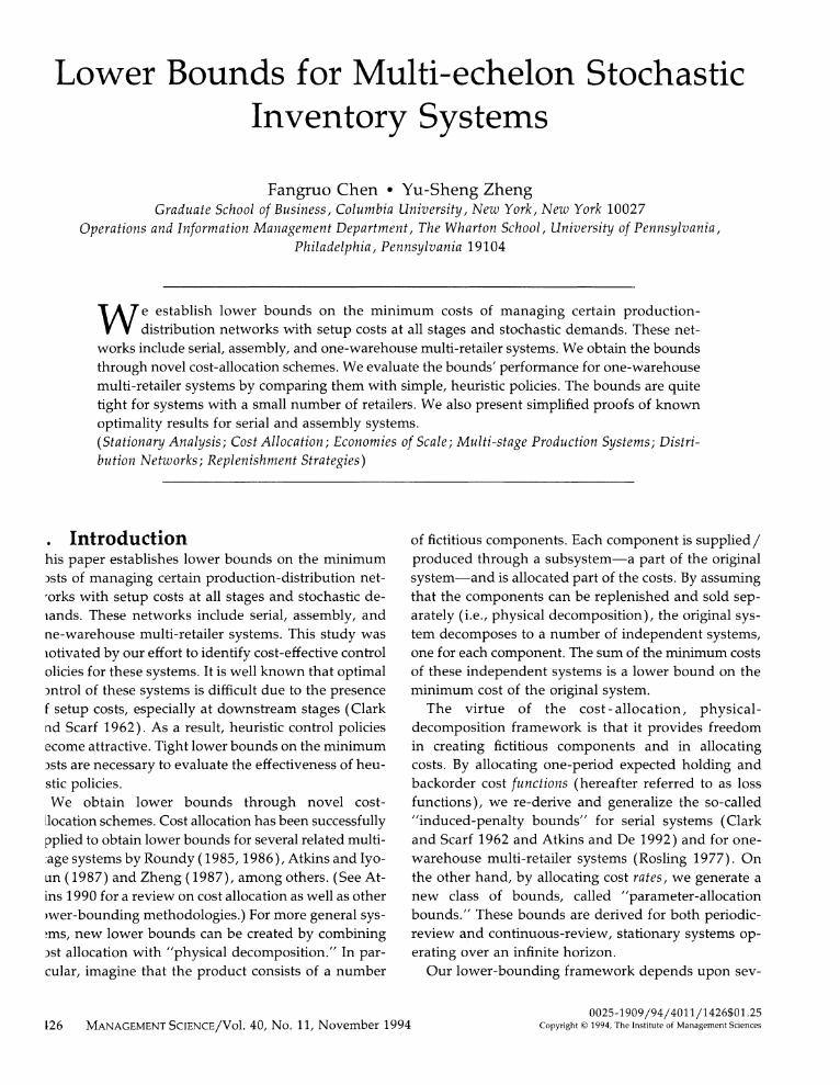
Component i is directly shipped from an outside supplier to retailer i. Allocate setup cost Ki (i = 0, . . . , N) to component i and warehouse echelon holding cost rate ho to component 0. The loss function at retailer i, Gi ( * ), is allocated between component 0 and component i: Gi(*) to component 0 and Gi(*) to component i. In summary, the system of component 0 is Distri- bution(N, KO) with warehouse echelon holding cost rate ho (assessed on the warehouse echelon inventory level), loss function G? (*) at retailer i (assessed on the inventory position of retailer i). The system of component i = 1, . . . , N is a single-stage system with setup cost Ki, loss function G (.). The component systems are depicted in Figure 3.

In the original system, replenishment of the components is "coordinated": when a shipment of component 0 is released at the warehouse to retailer i, a same quantity of component i is released at a supplier to retailer i. Both shipments arrive at retailer i at the same time. After arriving at the retailer, components 0 and i are sold in packages. Now assume that the components can be replenished and sold independently of each other. As a result, the original system decomposes to N + 1 component systems. The minimum cost of component i = (1, . . . , N) is Ci (Appendix A). A lower bound on the minimum cost of component 0, Co, can be obtained by replacing Gi ( * ) in (B5) in Appendix B with G? (.). Therefore, a lower bound for Distribu- tion(N) is

N

def= i C ip = 2: ci i=O

Figure 3 Decomposition of Distribution (N)

System of Systems of

Distribution(N) Component 0 Components 1,...,N

(Rosling (1977) obtained precisely this bound in a different form, but only under additional technical conditions.)

4.2. Parameter-allocation Bounds The previous subsection established induced-penalty bounds by allocating loss functions, or "expected" costs. Next we derive a new class of lower bounds for Se- ries (N), Assembly (S), and Distribution (N) by allocating "real" costs, i.e., holding and backorder cost rates.

4.2.1. Series(N). First consider Series(2). Create fictitious components and their systems as in Figure 1. Allocate setup cost Ki (i = 1, 2) to component i and echelon holding cost rate h2 to component 2. The echelon holding cost rate h, and the backorder cost rate p at stage 1 are allocated between components 1 and 2: h} and p' to component 1; h 2 and p2 to component 2. The allocated cost rates satisfy h 1 + h 2 = hi and pl + p2 = p. Check that the sum of the allocated costs of the components is equal to the total cost of the original system. Since the minimum costs for components 1 and 2are C'(K1, hI, p', Ll, F) and C'(K2, h , h2, p2 ILl, L2, F) respectively, a lower bound on the minimum cost of Series( 2) is

Cs(K1, h}, p', L1, F) + Cs (K2, h 2, h2, p2, L1, L2, F).

Consider the special cost allocation with h 2 = 0. Ex- amine the system of component 2. In this case, since there is no setup cost or echelon holding cost at stage 1, there is no incentive to keep any stock at stage 2. In other words, the system of component 2 effectively reduces to a single-stage system with setup cost K2, holding cost rate h2, backorder cost rate p l, and transportation leadtime L, + L2. Notice that holding costs start to accumulate at rate h2 as soon as the component enters the system (at stage 2). The time for each unit of the component to go from stage 2 to stage 1 is L, periods, during which a holding cost of h2L1 is incurred. Con- sequently, the long-run average holding cost incurred while shipping the component from stage 2 to stage 1 is gth2L, per period, where ,u is the mean one-period demand. In summary, under the above cost allocation the parameter-allocation bound becomes

Cs(K1, hi, p', L1, F)

+ Cs(K2, h2, p2, L2 + L1, F) + gh2Li.

1436 MANAGEMENT SCIENCE/VOL 40, No. 11, November 1994


With the above illustration, constructing a lower bound for Series(N) becomes straightforward. Suppose that there are N fictitious components, denoted by 1, ... , N. The system of component j is Series (j, Kj) with echelon holding cost rate h at stage i, i = 1, . . .,

and backorder cost rate p i (at stage 1). The cost allocation satisfies INi h j = hi for i = 1, ..., N and Z=1 pJ = p. Notice that the minimum cost for component j is

Cj,(Kj, h', p', LI, F),

where h h {h } j=1 and L = {L} j . A lower bound on the minimum cost of Series(N) is simply the sum of the minimum costs of all the components.

4.2.2. Assembly(S). From ?3, we know that it is straightforward to compute the minimum cost of an assembly system with a setup cost only at its highest stage, the stage with the longest total leadtime. Since there is a setup cost at each stage in Assembly(S), a natural approach is to decompose the system into sub- systems of Assembly(g, K)-type.

Recall that there are N stages in Assembly(S9). The stages are numbered in increasing order of total leadtimes. (Thus stage N has the longest total leadtime.) Imagine that the end product consists of N fictitious components. Consider component j (= 1, . . . , N). Delete stages j + 1, . . ., N of S. The resulting graph is still a tree, denoted by gj with gN = ?. Component j is produced through gj. Allocate Kj to stage j, echelon holding cost h j to stage i (=1, . .. , j), and backorder cost pi to stage 1. The cost allocation satisfies I N i h = hi for i = 1, . . ., N and E1 p - p. The system of component j is of Assembly(9j, Kj) -type, with minimum cost

C I(Kj, h', p'. LI, F)

whereh= { h j } i and Li = {L }i. The sum of these minimum costs over all components is a lower bound on the minimum cost of Assembly (S).

4.2.3. Distribution(N). Create fictitious components as in ?4.1.3, but allocate costs differently. The system of component 0 is Distribution (N, KO) with echelon holding cost rate ho at the warehouse, and echelon holding cost rate hi and backorder cost rate pi at retailer i. The system of component i = 1, . . . , N is a single-stage system with setup cost Ki, holding cost

rate hi, backorder cost rate p . The cost allocation sat- isfiesh +h? =hiandp +p? =pifori= 1,...,N. Recall that the minimum cost of component 0 is unknown, but a lower bound on it is

CN(Ko, ho, h0, p0, L, F),

whereh? = {h }I and po = {p? }I . The minimum cost of component i = 1,.. .,N is

Cj(Ki, hi, pi, Li, Fi)

where Fi is the cdf of one-period demand at retailer i. Consequently, the sum of the minimum costs of components 1, ... , N and the lower bound of component 0,

N

CN(Ko, ho, h0, p0, L, F) + Z Cs(Ki, hi, pi, Li, Fi), i=l

is a lower bound on the minimum cost of Distribu- tion (N). For easy reference, write CPa for the maximum value of the above expression over all possible cost allocations. (In the above cost allocation, we should re- strict p9 > 0 for all i in order to prevent the lower bound for component 0 from becoming negative infinity. But h? is allowed to be negative so long as h? + ho 2 0.)

It is interesting to contrast our approach here with the bounding scheme of Atkins and lyogun (1987) for one-warehouse multi-retailer systems with deterministic demand. In their approach, the warehouse setup cost is allocated to decompose the system into a number of two-stage, serial systems. However, as recognized by Atkins (1990), this method fails for not capturing the "risk pooling" function of the warehouse when demand is stochastic. Our method overcomes this difficulty: we preserve the warehouse node leaving its risk-pooling function intact but decompose the retailer nodes.

4.3. Integrated Bounds We have obtained induced-penalty bounds by allocating loss functions and parameter-allocation bounds by allocating cost rates. These allocation schemes can be integrated to generate a class of dominant bounds. We use Distribution(N) as an illustration.

First, create fictitious components and allocate cost rates as in ?4.2.3. Let A denote an allocation of the holding and backorder cost rates, i.e., hi, hi? pi and p? with hi + hi? = hi and pi + p?9 = pi for 1 c i c N. Under A, the loss function for component i is

MANAGEMENT SCIENCE/VOL. 40, No. 11, November 1994 1437

CHEN AND ZHENG Lower Bounds for Multi-echeloni Stochastic Inventory Systems

def

Gi(ylA) = E{hi(y - Di[t, t + Li])+

+ p(y - Di[t, t + Li])}

and the loss function for retailer i in the system of component 0 is

G(yfA) E E{h?(y - Di[t, t + Li])

+ (ho + p9)(y - Di[t, t + Li]y}

The system of component i = 1,... , N is a single-stage system with setup cost Ki, loss function Gi (I * A), and the demand process of retailer i. Since Gi ( * A) is convex, (s, S) policies are optimal for the system. Let si (A) be the optimal reorder point and Ci (A) the minimum cost. Note that Ci((A) = Cs(Ki, hi, pi, Li, Fi), where Fi is the cdf of one-period demand at retailer i.

Now allocate loss functions. For i = 1, . . . , N, define

{Ci(A) if y?csi(A) Gii(y I A ) =

j() i y<S A

G ) Gi (y I A) otherwise

and Gio(yjA) = Gi(y A) - Gii(yjA). Allocate Gi0( j A) back to component 0. With this allocation, component i's loss function (1 ' i ' N) reduces from Gi( IA) to Gii( 1A), but its minimum cost remains unchanged at C, (A) (Appendix A). On the other hand, the loss-function allocation increases the loss function of component 0 at retailer i from G 9( IA) to GI( IA) + Gio( 1A). As a result, the lower bound for component 0, denoted by Co(A), is greater than CN(Ko, ho, ho, p0, L, F), the lower bound for component 0 before allocating loss functions. (C0(A) is obtained by replacing Gi ( * ) in (B5) of Appendix B with G?(. IA) + Gio( IA).) Therefore, by allocating cost rates as well as loss functions, we have a new lower bound for Distribution(N):

N

I Ci(A) i=O

The integrated bound, denoted by C, is the maximum value of the above expression over all possible allocations A. (In ?4.2.3, we mentioned that p9 should be restricted to be nonnegative. This restriction should not be used in computing the integrated bound. To see this, consider the system of component 0. Recall that under the above integrated cost allocation, the loss function at retailer i is [G 9(y IA) + Gio(y IA)], whose slope is always -(pi + ho) as y -oo regardless what p9 is. In

other words, a unit of backorder at retailer i ultimately increases cost by (pi + ho). On the other hand, since the echelon holding cost at the warehouse is assessed on the warehouse echelon inventory level, a unit of backorder at retailer i decreases cost by ho. Thus the net penalty of a backorder at retailer i is pi. Therefore, no matter what the value of p? is, a positive penalty is incurred for each additional unit of backorder.)

From the above derivation, it is clear that C 2 CPa. It is also true that C 2 C'P. To see this, consider the following allocation of cost rates A0: hi = hi, hi = 0, pi = pi + ho, and p? = -ho. Under A0, check that IN1=o Ci (- A) = C'P. Therefore,

THEOREM 3. C 2 max{ CPa, Cip}.

5. Extension to Continuous-review Systems

We have so far focused on periodic-review systems. Parallel results can be obtained for their continuous- review counterparts with compound Poisson demand. These include the optimality results of ?3 and the lower bounds of ?4.

The definitions of the periodic-review systems in ?2 can be easily adapted for their continuous-review counterparts. The constant transportation leadtimes can now take any nonnegative values. In a continuous- review system, the holding and backorder costs accrue continuously over time at rates proportional to inventory levels. Therefore, the cost rates hi's and pi's should be re-defined as costs per unit time. Furthermore, since a continuous-review system monitors its inventory status continuously and can make replenishment decisions at any time, the time index t in the state variables, e.g. IPi (t), can be any time epoch.

From the previous development, we see that a key building block for our results is that (s, S) policies are optimal for single-location, periodic-review systems. Fortunately, a similar result also holds for single- location, continuous-review systems with compound Poisson demand (Beckmann 1961). To extend the previous results for periodic-review systems to their continuous-review counterparts with compound Pois- son demand, we only need to notice that: (a) the compound Poisson demand process is memoryless (this property is parallel to the iid-demand assumption for periodic-review systems); (b) the loss functions for

1438 MANAGEMENT SCIENCE/VOL. 40, No. 11, November 1994


Figure 4 Frequency Diagrams of the Ratios of Parameter-Allocation Bounds to Induced-Penalty Bounds for Distribution (N). The Horizontal Axes Represent the Ratios in Percentage

N=1 N=4 140- 140

120 120

-? 100 1 100

E E (a (a X 80- X 80.

w0 w

o o so-6 so.W

0)0

E E 40 - 40- z z 20, 20-

0 0 . . . . .. . . . . . . . . . 90 93 96 99 102 106 108 90 93 96 99 102 105 108

N=8 N=16 140- 140-

120- 120-

-e 100- CD 100- 0. 0 E E X 80X 8 w w o 0 L. 60 6- W0 CD e

.0 . E E

40 - 40-

z z 20- 200 ** IIIiEI

90 93 96 99 102 105 108 90 93'96t'90 102 105 108

N=32 140-

120-

-~100-

E kV X 80- w 0

00

E 40- z

20-

90 93 90 99 102 106 108


periodic-review systems are now loss rate functions; and (c) the idea of cost allocation/ physical decomposition does not depend on the inventory review system in place.

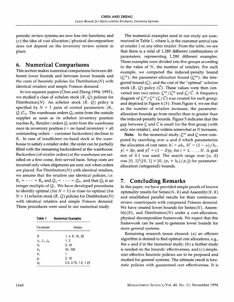
6. Numerical Comparisons This section makes numerical comparisons between different lower bounds and between lower bounds and the costs of heuristic policies for Distribution (N) with identical retailers and simple Poisson demand.

In two separate papers (Chen and Zheng 1994, 1993), we studied a class of echelon stock (R, Q) policies for Distribution (N). An echelon stock (R, Q) policy is specified by N + 1 pairs of control parameters: (Ri, Qi )N=o. The warehouse orders Qo units from the outside supplier as soon as its echelon inventory position reaches Ro. Retailer i orders Qi units from the warehouse once its inventory position (= on-hand inventory + all outstanding orders - customer backorders) declines to Ri. In case of insufficient on-hand stock at the warehouse to satisfy a retailer order, the order can be partially filled with the remaining backordered at the warehouse. Backorders (of retailer orders) at the warehouse are sat- isfied on a first-come, first-served basis. Setup costs are incurred only when shipments are sent, not when orders are placed. For Distribution (N) with identical retailers, we assume that the retailers use identical policies, i.e. R1 = = RNand Ql = * = QN, and that Qo is an integer multiple of Ql. We have developed procedures to identify optimal (for N = 1) or close-to-optimal (for N > 1) echelon stock (R, Q) policies for Distribution(N) with identical retailers and simple Poisson demand. These procedures were used in our numerical study.

Table 1 Numerical Examples

Parameter Values

N 1, 4, 8, 16, 32 /\,, Ll, Lo 1, 2 K1 5, 10 Ko 50, 100 h1 1

Pi 5, 10 0.5, 0.75, 1.0, 1.25

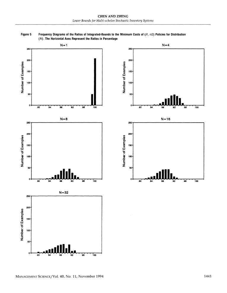
The numerical examples used in our study are sum- marized in Table 1, where Al is the customer arrival rate at retailer 1 or any other retailer. From the table, we see that there is a total of 1,280 different combinations of parameters, representing 1,280 different examples. These examples were divided into five groups according to the value of N, the number of retailers. For each example, we computed the induced-penalty bound (CiP), the parameter-allocation bound (CPA), the integrated bound (C), and the cost of the "optimal" echelon stock (R, Q) policy (C). These values were then con- verted into two ratios: CPa/C'P and C/ C. A frequency diagram of CPa/CiP (C/ C) was created for each group, and depicted in Figure 4 (5). From Figure 4, we see that as the number of retailers increases, the parameter- allocation bounds go from smaller than to greater than the induced-penalty bounds. Figure 5 indicates that the gap between C and C is small for the first group (with only one retailer), and widens somewhat as N increases.

Note. In the numerical study, CPA and C were computed by searching over a and : which parameterize the allocation of cost rates: h' = ahl, h? = (1 - a)/hl, p, =flp, and p2 = (1 -f)plfori= 1,..., N. Agrid size of 0.1 was used. The search range over (a, A) was [0, 1]2([0, 1] X [0, (pi + ho)/p1]) for parameter- allocation (integrated) bounds.

7. Concluding Remarks In this paper, we have provided simple proofs of known optimality results for Series (N, K) and Assembly( (, K) and established parallel results for their continuous- review counterparts with compound Poisson demand. We have created lower bounds for Series(N), Assem- bly(?), and Distribution(N) under a cost-allocation, physical-decomposition framework. We expect that this framework can be used to generate lower bounds for more general systems.

Remaining research issues abound: (a) an efficient algorithm is desired to find optimal cost allocations, e.g., the a and : in the numerical study; (b) a further study is needed on the bounds' effectiveness; and (c) simple, cost-effective heuristic policies are to be proposed and studied for general systems. The ultimate result is heuristic policies with guaranteed cost effectiveness. It is



Figure 5 Frequency Diagrams of the Ratios of Integrated-Bounds to the Minimum Costs of (R, nQ) Policies for Distribution (N). The Horizontal Axes Represent the Ratios in Percentage

N=1 N=4 250 250C

200? 2001

Q o

E E 0 150 kV 150| x x

o o

0) 100U 02 1000 .0 .0 E E z z

50 80.000

. 0 . . . . . . 80 84 88 92 96 100 80 84 8 92 96 0

N=8 N 1 6 250- 250-

200' 200-

0 0

E E to 150- CO 150- x x w w o 0 e 100 0 100-

E E z z

50 so.

so 8410 820.s 4 g 6 100

N=32 250-

200-

(D

E x

0 0) 100.

.0 E z

50-

80 84 88a 92 96 100

CHEN AND ZHENG Lower Bounds for Multi-echelon Stochastic Inventory Systenms

our hope that the results presented in this paper will serve as a stepping stone in this endeavor.1

1 The authors would like to thank the Associate Editor and two referees for their constructive comments that have led to many improvements in the exposition of this paper. This research was supported in part by NSF grant DDM 9111183.

Appendix A Consider a single-location, periodic-review system with infinite plan- ning horizon. Demands in different periods are independent and identically distributed with one-period probability mass function pj, j = 0, 1, .... It has setup cost K and loss function G(*) (a function of its inventory position). The long-run average cost of an (s, S) policy in this system is

K ? sS-4 G(S -j)m(j) C(S, S) = S-m-l

Ej=o m(l)

where

m (O) = 1_ p and m(i)= Z pjm(i-j) i = 1, 2, * * . lPo 1~~~~~~=0

Let Y be the minimizer of G(.). It follows from Zheng (1991) that there exists an (s*, S*) policy that satisfies

def (i) g* = c(s*, S*) = mins<s c(s, S)

(ii) s* < Y S*

(iii) G(s* + 1) ? g* c G(s*)

(iv) g* 2 G(S*). Define

G(i) i > s* G-(i) =

Now modify the above system by replacing the loss function G(*) with G-(.). The long-run average cost of an (s, S) policy in this modified system is

K + s-s- G-(S - j)m(j) C(S, 5) =

= S-s-1

2:j=0 m(j)

LEMMA. g* = mins<s c(s, S).

PROOF. First notice that c-(s*, S*) = g*. Thus we only need to show that c(s, S) 2 g* for all s < S. Take any s < S. Consider the following cases: (1) If s 2 s* then c(s, S) = c(s, S) > g*; (2) if s < S* and S ? s* then

K + g* z Ss1(j) C(S, S) - S-- mj g

2:j=o m(l) and (3) if s < s* and S > s* then

c-(s, S) = wc(s*, S) + (1 - w)g* > g*

where w = s-s- m(I)/ 0 m(j) E (0, 1], and the inequality follows since c (s *, S) > g*.

The above lemma shows that the (s *, S *) policy satisfying conditions (i)-(iv) is the optimal (s, S) policy for the above modified system (with loss function G-(*)). In fact, this policy is optimal among all policies.

THEOREM. The (s*, S*) policy is optimal for the modified systemn.

PROOF. Analogous to Theorem 2 of Zheng (1991). 0

Appendix B Based on Federgruen and Zipkin (1984a, b, c), here we briefly derive CN(K, h, p, L, F). Consider any feasible policy in Distribution(N, K). The total systemwide holding and backorder costs at period t are

N

hoIo(t) + hi Ii (t) + pi Bi (t)] i=l

Since ILO ( t) = IO( t)- i= 1 Bi ( t), the above expression can be written as

N

hoILo(t) + [hiIi(t) + (ho + pi)Bi(t)] i=l

For convenience, we charge the following to period t:

N

hoILo(t) + E [hiIi(t + Li) + (ho + pi)Bi(t + Li)]. (Bi)

It is clear that this cost accounting scheme will not affect the long- run average systemwide holding and backorder costs. Recall that IL-(t) is the beginning echelon inventory level at the warehouse at period t (before demand occurrence). Thus ILo (t) = IL - (t) - Do[ t, t]. Consequently, (Bi) becomes

ho { IL-(t) - Do[t, t] }

N

+ E [hiIi(t + Li) + (ho + pi)Bi(t + Li)]. (B2) i=l

Notice that Ii(t + Li) = {IPi(t) - Di[t, t + Li]}+ and Bi(t + Li) = {IPi(t) - Di[t, t + Li]}. Given ILj-(t) = y and IPi(t) = yi for

=1, . . ., N, the expected value of (B2) is

N

ho (y - sO) + Gi (yi) (B3) i=l

where AtO is the mean one-period system demand and def

Gi(y) = E[hi {y-Di[t, t + Li }+

+ (ho + pi){y-Di[t, t + Li]}-], (B4)

the loss function for retailer i. Notice that, by definition, the total inventory position of the retailers

cannot exceed the beginning echelon inventory level at the warehouse, i.e., i yN ? y. Thus for any given value of y, a lower bound on (B3) is

def N R(y) = ho(y - io) + min Gi(yi). (B5)

Ni -1 iyi


CHEN AND ZHENG Lower Bounds for Multi-echelon Stochastic Inventony Systems

In other words, given that the beginning echelon inventory level at the warehouse is y, the expected one-period holding and backorder costs are at least R(y). Notice that R( * ) is convex and easy to compute (cf. Zipkin 1984 for further references). The minimization in (B5) is effectively a free inventory position rebalance, a technique used by Eppen and Schrage (1981) and Federgruen and Zipkin (1984a, b, c) in solving what they called the myopic allocation problem.

Notice that IL-(t) = IPo(t - Lo) - Do[t - Lo, t). Hence, given IPO(t - Lo) = z, the expected system-wide holding and backorder costs charged to period t are at least

def Go(z) = ER(z - Do[t - Lo, t)).

Since R(*) is convex, Go(-) is convex. By substituting Go(z) for the expected system-wide holding and backorder costs at period t, the original system reduces to a single-location system with setup cost K, loss function Go( * ), and the aggregate demand of the original system. Since Go( ) is convex, (s, S) policies are optimal for the single-location system. The cost of the optimal (s, S) policy is Cd (K, h, p, L, F).

References Atkins, D., "A Lower Bound to the Dynamic Assembly Problem,"

Working Paper No. 1259, Faculty of Commerce and Business Administration, The University of British Columbia, Vancouver, B.C., Canada, 1988. , "A Survey of Lower Bounding Methodologies for Production/ Inventory Models," Annals of Oper. Res., 26 (1990), 9-28. , and S. De, "94% Effective Lot-Sizing for a Two-Stage Serial Production/ Inventory System with Stochastic Demand," Work- ing Paper, Faculty of Commerce, University of British Columbia, Vancouver, B.C., Canada, 1992. and P. lyogun, "A Lower Bound on a Class of Coordinated

Inventory/Production Problems," 0. R. Letters, 6 (1987), 63- 67.

Beckmann, M., "An Inventory Model for Arbitrary Interval and Quantity Distributions of Demand," Maniagemenit Sci., 8 (1961), 35-57.

Chen, F. and Y. S. Zheng, "Evaluating Echelon Stock (R, nQ) Policies in Production/Inventory Systems with Stochastic Demand," Management Sci., 40 (1994), 1262-1275. and , "One-warehouse Multi-retailer Systems with Cen-

tralized Stock Information," Working Paper, Department of De- cision Sciences, The Wharton School, University of Pennsylvania, 1993.

Clark, A. J. and H. Scarf, "Optimal Policies for a Multi-Echelon In- ventory Problem," Management Sci., 6 (1960), 475-490. and , "Approximate Solutions to a Simple Multi-Echelon

Inventory Problem," in Studies in Applied Probability and Man-

agemnent Science, pp. 88-110. K. J. Arrow, S. Karlin and H. Scarf (Eds.), Stanford University Press, Stanford, CA, 1962.

Eppen, G. and L. Schrage, "Centralized Ordering Policies in a Mul- tiwarehouse System with Lead Times and Random Demand," in Multi-Level Production/Inventory Control Systems: Theony and Practice, L. Schwarz (Ed.), North-Holland Publishing Company, Amsterdam, 1981.

Federgruen, A. and P. Zipkin, "Approximation of Dynamic, Multi- Location Production and Inventory Problems," Management Sci., 30 (1984a), 69-84. and , "Computational Issues in an Infinite Horizon, Multi-

Echelon Inventory Model," Oper. Res., 32 (1984b), 818-836. and , "Allocation Policies and Cost Approximation for Multi- Location Inventory Systems," Naval Res. Logist. Quart., 31 (1984c), 97-131.

Iglehardt, D., "Optimalities of (s, S) Inventory Policies in the Infinite Horizon Dynamic Inventory Problem," Management Sci., 9 (1963), 259-267.

Rosling, K., "A Generalization of Clark and Scarf's Approach to Multi- Echelon Inventory Control," in Three Essays on Batch Production and Optimization, Linkopings Tryckeri AB. Linkoping, Sweden, 1977. , "Optimal Inventory Policies for Assembly Systems Under Ran- dom Demands," Oper. Res., 37 (1989), 565-579.

Roundy, R. O., "98% Effective Integer-Ratio Lot-Sizing for One- Warehouse Multi-Retailer Systems," Management Sci., 31 (1985), 1416-1430. ,"A 98% Effective Lot-Sizing Rule for a Multi-Product, Multi- Stage Production Inventory System," Math. Oper. Res., 11 (1986), 699-727.

Scarf, H. E., "The Optimalities of (s, S) Policies in the Dynamic In- ventory Problem," in Matheniatical Methods in the Social Sciences, K. Arrow, S. Karlin and P. Suppes (Eds.), Stanford University Press, Stanford, CA, 1960.

Veinott, A., Jr., "On The Optimality of (s, S) Inventory Policies: New Conditions and A New Proof," SIAMJ. Appl. Math., 14 (1966), 1067-1083. and H. Wagner, "Computing Optimal (s, S) Inventory Policies," Maniagement Sci., 11 (1965), 525-552.

Zheng, Y. S., "Replenishment Strategies for Production/ Distribution Networks with General Joint Setup Costs," Ph.D. Dissertation, Columbia University, New York, 1987. , "A Simple Proof for the Optimality of (s, S) Policies for Infinite Horizon Inventory Problems," J. Appl. Prob., 28 (1991), 802- 810. and A. Federgruen, "Finding Optimal (s, S) Policies is About as Simple as Evaluating a Single Policy," Oper. Res., 39 (1991), 654-665.

Zipkin, P., "On the Imbalance of Inventories in Multi-Echelon Sys- tems," Math. Oper. Res., 9 (1984), 402-423.

Accepted by Azwi Federgruen; received August 23, 1991. This paper has been with the authors 7 months for 3 revisions.


Documents

Lower Bounds for Multi-Echelon Stochastic Inventory Systems