Embed Size (px)
Citation preview

Auton RobotDOI 10.1007/s10514-016-9591-z
Low stiffness design and hysteresis compensation torque controlof SEA for active exercise rehabilitation robots
Wonje Choi1 · Jongseok Won1 · Jimin Lee1 · Jaeheung Park1,2
Received: 3 April 2015 / Accepted: 25 June 2016© Springer Science+Business Media New York 2016
Abstract Rehabilitation robots for active exercise requirescompliant but consistent torque (or force) assistance (orimposition) while passive rehabilitation robots are pro-grammed to execute certain movements for patients. Thiskind of torque assistance in the rehabilitation system canbe provided by using SEA (Series Elastic Actuator). In thispaper, low stiffness SEA and spring hysteresis compensa-tion are proposed for the robust and accurate torque controlof the rehabilitation robot. C-DSSAS (Compact Dual SpiralSpring Actuation System) is developed to implement the lowstiffness SEA and a hysteresis compensation method is pro-posed for robust accurate torque control. Pros and cons of lowstiffness SEAs are dealt with in order to explain validity ofproposed application. In addition, proposed hysteresis com-pensation torque controller has backlash-based polynomialmodel and passivity-based control. Experiments of activeexercise of kneewere performedwearing the knee rehabilita-tion device using the C-DSSAS with hysteresis control. Theexperimental results demonstrate its improved performanceof the robot in terms of the robustness and accuracy.
B Jaeheung [email protected]
Wonje [email protected]
Jongseok [email protected]
Jimin [email protected]
1 Department of Transdisciplinary Studies, Seoul NationalUniversity, Seoul, Republic of Korea
2 Advanced Institute of Convergence Science and Technology,Suwon, Republic of Korea
Keywords Rehabilitation robots · Series elastic actuator ·Spiral spring · Hysteresis · Low stiffness · Passive basedcontrol · Backlash model
1 Introduction
This paper deals with SEA(Series Elastic Actuator) ofrehabilitation robots for active exercises such as strengthexercises, weight supported walking, etc. Active rehabilita-tion exercises are described above all as a proposed appliationof low stiffness SEAs, then SEAs for rehabilition robotsare reviewed. It is described through contrast with passiveand active-assistive exercises robots, because existing robotshave been mainly developed for those kind of exercises.
1.1 Active and passive exercises
Rehabilitation exercises are divided into active, passive, andactive-assistive exercises in accordance with the degree ofvoluntary muscle control (Andrews et al. 2011). Generalexercises such as strength training, endurance training, aero-bic exercises, and flexibility exercises performed by healthypeople as well as rehabilitation patients are included inthe active exercise. Mainly aimed at the patient, the pas-sive and the active-assistive exercises are fully or partiallyperformed by physical therapists. Proprioceptive neuro-muscular facilitation techniques, restoring range of motion(ROM) techniques, and task-specific training are types ofthese exercises (Voight et al. 2006).
Rehabilitation robots have mainly been developed forpassive and active-assistive rehabilitation exercises, becauserobots enable patients to perform stable rehabilitation exer-cises by replacing the hard and continuous physical efforts oftherapists. Typical robots for these exercises are gait training
123
Auton Robot
robots for patientswith diseases related to the nervous systemsuch as stroke and spinal cord injury (SCI). Treadmill gaittrainers such as Lokomat (Colombo et al. 2000) , LokoHelp(Freivogel et al. 2008), ReoAmbultor (West 2004), LOPES(Veneman et al. 2007), and foot-plate-based gait trainers(Díaz et al. 2011) such asGangtrainerGT I (Hesse et al. 2000)and HapticWalker (Schmidt 2004) are among these robots.These robots have been developed for task-specific training,which is carried out with repeated walking motion. Rewalk(Goffer 2006) is an over-ground gait trainer. The robot is notdesigned to repeat gait motion, but enables patients to walkwith programmed gait trajectories. Physiotherabot (Akdoganand Adli 2011) is a versatile robot manipulator for lowerlimbs. One of the functions of this robot is passive exercisesfor recovering ROM.
These robots largely use position control employed fortracing motion trajectories and impe-dance control exploitedin addition to position control for reflecting intention of exer-ciser. They have sufficiently large torque and high impedanceperformance to support human users. Therefore, the robotscan fully or partially involve human motor control.
On the other hand, rehabilitation robots for active exer-cises do not involve the motor control of the exercisers,but control their exercise load for safe and adequate exer-cise. Representative examples of the robots include bodyweight support systems. These reduce the exercise loadsand the stress on the exercisers joints. Zero-G (http://www.aretechllc.com/) is a weight support system for gaittraining. The SEA of this system applies gravity com-pensation force to support weight. Alter-G (http://www.alterg.com/) was developed for aerobic exercises such aswalking and running. Air pressure from the device gen-erates lifting force for the exerciser. The body weightsupport systems of the above-mentioned gait trainers havethe same function as these robots, though they are not foractive robots. The Lokolift (Frey et al. 2006) of LOPES(Veneman et al. 2007) is one of them, and it employsthe principle of SEA for applying support force. On thecontrary to these robots, robots can apply exercise loadsfor active exercises. This function of the robots can beused for strength exercises. Strength training is dividedinto isotonic, isometric, and isokinetic exercises in accor-dance with forms of muscle contraction. In the case ofisometric exercise and isokinetic exercise, the robot keepsits position, and the exerciser applies force or torque tothe robot. Meanwhile, the robot applies load force ortorque to the exerciser in isotonic exercises. The System4 Pro (http://www.biodex.com/physical-medicine/products/dynamometers/system-4-pro) is an apparatus for isokineticexercise, and it can also be used for isometric and iso-tonic exercise. The previously mentioned Physiotherabot(Akdogan andAdli 2011) also has functions of these strengthexercises.
The rehabilitation robots for body weight support systemsor isotonic strength exercises are controlled by force andtorque controllers. These robots interact directly with humanexercisers with the final output of force (or torque). There-fore, robust and stable controls of robots are important tothe safety and comfort of the exercisers, especially weak orelderly patients. We focus on design and control methods forrobust and accurate control.
1.2 SEA for rehabilitation exercises
SEA is a compliance actuator (Ham et al. 2009) that cou-ples a spring and an actuator in series. This actuator hasbeen applied to rehabilitation robots for various purposesbecause of its compliance and advantages for torque con-trol. Roboknee (Pratt et al. 2004), RSEA (Kong et al. 2009),CompAct-ARS (Karavas et al. 2012), and compact rotarySEA (Sergi et al. 2012), among others, have been developedas assistivewearable robots, and robots such as LOPES (Ven-eman et al. 2007) and eSEAJ (Lagoda et al. 2010) have beendeveloped for gait training. In addition, the Powered Ankle-Foot prosthesis (Au et al. 2007), Clutchable SEA (Rouse et al.2013), and others have been developed as prosthesis robots.
Of these, LOPES is a representative robot that appliesSEA for passive and active-assistive exercises. In studies onthis robot, the SEA design and control method were stud-ied for those exercises. In particular, it was reported thatthe SEA should have a sufficiently high stiffness for theseapplications (Veneman et al. 2007) , because an SEA cannotachieve greater impedance than its mechanical stiffness inthe impedance control. For this reason, the stiffness of theSEA is 219 Nm/rad in LOPES and is known to have well-designed stiffness. Additionally, Rotary SEA (Sergi et al.2012) and eSEAJ (Lagoda et al. 2010) have stiffness valuesof 219 Nm/rad and 119 Nm/rad, respectively, in a similarrange.
Unlike the SEAs developed for existing rehabilitationrobots, we address the SEA for active exercise robots. Inactive exercise, the load control ability of the SEA hasan advantage compared to other existing methods such asweights and springs. This advantage was aleady discussed inthe study of the Lokolift (Frey et al. 2006), because weightscause large load errors owing to the inertia effect, and withsprings, it is not easy to regulate the load. With appropriatedesign and control methods, an SEA can implement a morerobust and accurate torque control. Through high-qualitytorque or force control, the rehabilitation exerciser can workout safely and gradually.
For these purposes, we propose a low-stiffness designand spring hysteresis compensation control in this paper.In Sect. 2, the advantage of the low-stiffness SEA designis described for active exercise. The appropriate applica-tions are introduced together in accordance with the limits of
123

Auton Robot
this method. In Sect. 3, the spring hysteresis compensationcontroller is addressed. The hysteresis characteristics of amechanical spring and the proper model based on the classicbacklash model and passivity-based controller are described.In Sect. 4, the mechanical design of a compact dual spiralspring actuation system (C-DSSAS) is introduced, and thespring design of its three spring modules for the experimentsis presented. In Sect. 5, the experimental results of the per-formance of torque control are presented. In Sect. 6, we willprovide discussion and conclusions for these works.
2 Low stiffness SEA and torque control
The key advantage of a low-stiffness design of a SEA isits robust torque control with the external movement of ahuman. Robust torque control means that unnecessary gen-erated torque is reduced in human-robot interaction. Wedescribe this advantage with an example of a SEA lineartorque controller, but the same is true of the proposed hys-teresis compensation controller. This is shown through theexperiments in Sect. 5.
2.1 Advantaged of low-stiffness design of a SEA
When the final output of a control is torque, not positionor impedance, the low-stiffness SEA design has two advan-tages. First, it makes torque control robust by reducing thetorque error influence due to externalmovement. Second, it isadvantageous in implementing a higher resolution of outputtorque than a high-stiffness design.
To illustrate the former, we will consider a linear torquecontroller of a SEA as shown in Fig. 1b. The SEA is assumedto be used for applying torque to the knee of a human whoperforms active exercise. With the constant 1
k for convertingthe torque value to a displacement, position controller C andplant G for a geared motor constitute the spring deformationcontroller, and its output displacement is θm . However, thisdisplacement is affected by the movement of the human kneewhen it deforms the spring. In the SEA, this is because thegearedmotor, spring, and human knee are connected in seriesas depicted in Fig. 1a. The spring as a plant of the SEA con-verts spring deformation θs to output torque τ amplified byspring stiffness k. The movements of the human thus affectthe final output torque through the amplification of the plant.In other words, the interactive movements with human actsas a disturbance in the torque control, and this disturbance isamplified by the stiffness of the SEA. Equation (1) describesthe torque error of the torque controller in Fig. 1. As pre-viously mentioned, we can see that torque error is affectedby the product of human motion and spring stiffness, as wellas the position controller, geared motor plant, and referencetorque.
(a)
(b)
Fig. 1 A linear torque controller of SEA. a An example in which aSEA applies torque on knee. b A block diagram of the SEA’s lineartorque controller; k : spring stiffness, C : position controller, G : plantof geared motor, τre f : reference torque, τerr : torque error , τ : outputtorque, θm : displacement bymotor, θh : displacement by humanmotion,θs : spring deformation
τerr = 1
1 + CG· (τre f + k · θh) (1)
Whenwe try to increase the gain of the controller to reducethe torque error, it has the same limits irrespective of stiff-ness, because the system of the torque controller is the sameas the system of the geared motor position controller insidethe torque controller. This is due to the cancellation of thespring plant and the inverse of the stiffness constant as shownin Fig. 1. However, the increse of the gain can be limited byperformance of a geared motor of SEA if its stiffness is rel-atively low. It is described in the next subchapter.
The second advantage is related to the practical imple-mentation of the SEA. The resolution of an output torque ofa SEA depends on the resolution of a position sensor includ-ing an encoder for measuring the spring displacement. If it ispossible to implement a certain resolution on the maximumamount of spring deformation, there is no problem. However,in reality, it is difficult to implement sensors in this way,thus these characteristics are valid. From Hooke’s law, therelationship between the torque resolution ζ , displacementresolution ε of the position sensor for spring deformation,and spring stiffness k can be expressed as.
ζ = k · ε (2)
That is the lower stiffness can realize a higher torque reso-lution when measuring the spring deformation with the sameposition resolution. Furthermore, these features are effectivein reducing the torque control error.
123
Auton Robot
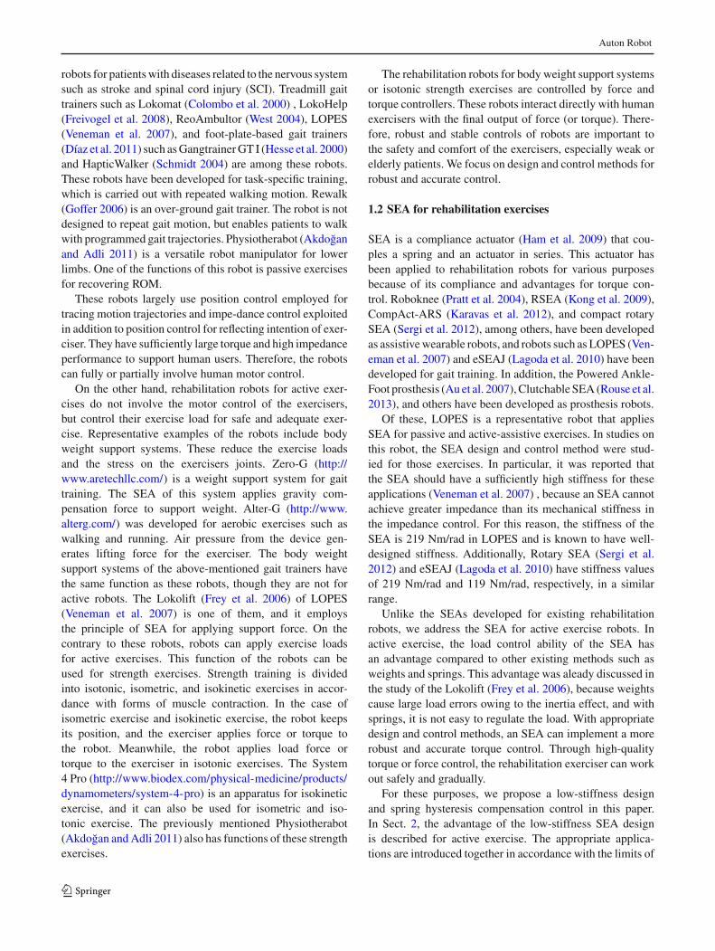
2.2 Disadvantages of low stiffness SEA design
A significant disadvantage of the low stiffness SEA design isthat the geared motor in SEA should cover wider spring dis-placement for the same torque output. Equation (3) describesthe relationship between output torque τ of SEA, spring stiff-ness k, spring deformation θs , displacement θm by the gearedmotor, and displacement θh by external motion of the human.This relationship is from Hooke’s law.
τ = k · θs = k · (θm + θh) (3)
From Eq. (3), we can derive a required displacement θm ,angular velocity ωm , and power Pm of the geared motor.Equations (4), (5), and (6) represent these respectively. Thevariableωh in Eqs. (5) and (6) represents the angular velocityby human motion.
θm = τ
k− θh (4)
ωm = 1
k· dτ
dt− ωh (5)
Pm = τ · ωm = τ ·(1
k· dτ
dt− ωh
)(6)
As shown inEq. (4), the lower stiffness of theSEArequiresmore displacement of the motor under the same torque andexternal movement. Equation (5) is obtained by differentiat-ing both sides of Eq. (4) for time. This relation indicates thatthe lower stiffness of SEAneeds a larger velocity for the sametorque gradient and external motion velocity. Therefore, therequired power is also increased if we use the lower-stiffnessspring for the SEA as depicted in Eq. (6). As a result, a gearedmotor with higher speed and power should be exploited inthe same torque requirement when we use a low spring stiff-ness for a SEA. This is consistent with the existing studyof LOPES (Veneman et al. 2006) that reported that too lowa SEA stiffness is limited in improving system bandwidth.Fromabove equations, one of important requirement for stiff-ness design is a torque rate for time. When the high torquerate is needed, a low-stiffness design of requires too higha specification of the motor from Eqs. (5) and (6). On theother hand, if there is no torque change required, spring stiff-ness is no longer a factor in increasing the speed and powerrequirements.
2.3 Proper application of a low-stiffness SEA
Despite the advantages discussed in the Sect. 2.1, the appli-cation of a low-stiffness SEA is limited by the disadvantagesdescribed in Sect. 2.2. Because of the high speed and powerrequirements of the motor, low-stiffness springs are not suit-able for portable robots such as light-weight wearable robots.
(a) (b) (c)
Fig. 2 Proper application of low stiffness SEA. a Weight supportdevice by prismatic SEA. b Weight support device by rotational SEA.c Strength exercise robot by rotational SEA
In addition, low stiffness is not a proper design option onaccount of the speed and power problems if a large torquerate is needed, such as for walking assistance. However, alow-stiffness spring for a SEA can be an appropriate designoption in the following cases:
a. Zero or sufficiently low torque (or force) rate require-ment.
b. Requirment of strict torque (or force) limitation.Case ‘a’ corresponds to applications such as body weight
support devices as shown in Fig. 2. In this case, the SEAapplies a constant weight compensation force to the human,thus, there is no force change rate. The low-stiffness draw-backs for speed and power requirement are no longer aproblem, and only the advantages are applicable. Case of‘b’ is applicable in cases of torque-based body weight sup-port robots for the closed-chain exercises in Fig. 2b andrehabilitation robots for the strength exercises in Fig. 2c. Inthese cases, the drawbacks for required speed and power ofa geared motor in SEA do not disappear completely. How-ever, a low-stiffness SEA can be considered sufficiently as adesign option in cases where relatively low torque rate andstict torque control, namely robust torque control, is requiredfor reasons such as safety, comfortability, etc. Strength exer-cises for patients whose muscle function is not completelyrecovered or exercisers who want stable gravity compensa-tion force by robots are suitable examples. These applicationsare consistent with those mentioned in the Sect. 1.
3 Hysteresis compensation torque control
For the accuracy of torque control, we propose a torque con-troller for compensating the hysteresis of springs. First ofall, the properties of spring hysteresis is introduced. Theunidirectional hysteresis characteristic of a single springand the bidirectional hysteresis characteristic of antagonisticinstalled springs are described by deformation experimentson a spiral torsion spring. Next, we propose a proper modelfor describing the quasi-static hysteresis characteristics of
123

Auton Robot
Fig. 3 Experiment Setup for measuring torque and displacement ofsprings
the SEA spring. Finally, the spring hysteresis compensationtorque controller is introduced. Its stability is analyzed byusing the concept of passivity. Experiments on the proposedcontroller are covered in Sect. 5.
3.1 Hysteresis characteristics of mechanical spring
As is well known from Hookes law, mechanical springs havea linear proportional relationship between force and dis-placement or torque and rotational displacement. In practice,however, they have non-linear characteristics. Hysteresisloops are caused by dissipation of elastic potential energy
due to internal friction, and non-linear relationships betweentorque (or force) and deformation are caused by unevenshapes or the number of active coils of springs.
Experiments for measuring the torque and displacementof springs were carried out to observe the static hysteresischaracteristics of springs. The experiments were conductedin the environment shown inFig. 3. Reference position trajec-tories are input to a servo motor, and the spring displacementand torque were measured by a 13-bit encoder (RMB28SC,RLS) mounted on a motor and a torque sensor (TCN 10K,Dacell) set up on a spring, respectively.
The experimental results for a single spring are shown inFig. 4. The spring used in the experiments is a spiral tor-sion spring designed and manufactured to have a stiffnessof 8.25 Nm/rad as a unidirectional spring. Figure 4b showsthe torque-deformation data of the spring for the input dis-placement trajectory shown in Fig. 4a. Experimental resultsindicate the unidirectional non-linear characteristics of thespring including hysteresis loops and non-linear curves.When velocity of displacement changes from positive to neg-ative, the torque value falls sharply in some displacementrange, then it falls gently after the range. These trajectoriesmake the hysteresis loops. This hysteresis of the mechanicalspring is relatively small compared to other materials suchas ferroelectric, magnetic, piezoelectric materials, etc. Insmall displacements, the relationship between deformation
0 50 100 150 200 250 300 350 400 450 500
Time (sec)
-1
-0.5
0
0.5
1
Ref
. Def
orm
atio
n (r
ad)
-1 -0.5 0 0.5 1
Deformation (rad)
-15
-10
-5
0
5
10
15
Tor
que
(Nm
)
0 50 100 150 200 250 300 350
Time (sec)
0
0.5
1
1.5
Ref
. Def
orm
atio
n (r
ad)
5.115.00
Deformation (rad)
0
1
2
3
4
5
6
7
8
9
10
Tor
que
(Nm
)
(a) (b)
(c) (d)
Fig. 4 Experiment results in respect of spring hysteresis. a Input trajectory for a single spring. b Result data of a single spring. c Input trajectoryfor bi-directional antagonistic connected springs. d Result data of bi-directional antagonistic connected springs
123
Auton Robot
(a) (b) (c)
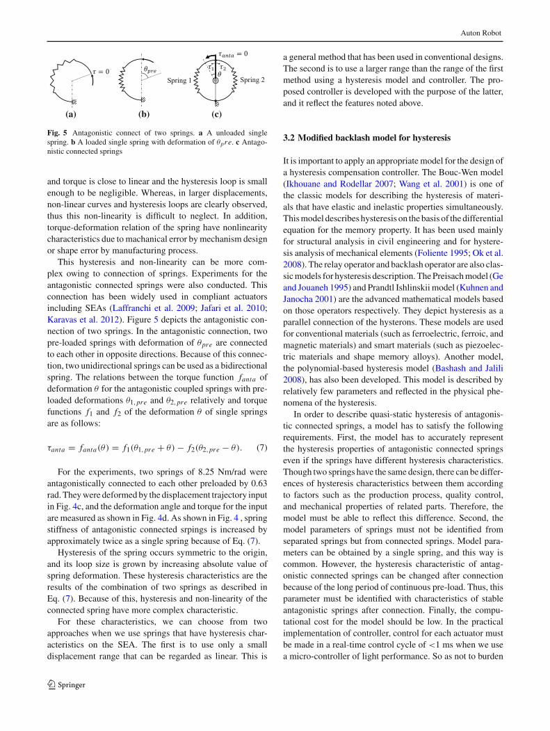
Fig. 5 Antagonistic connect of two springs. a A unloaded singlespring. b A loaded single spring with deformation of θpre. c Antago-nistic connected springs
and torque is close to linear and the hysteresis loop is smallenough to be negligible. Whereas, in larger displacements,non-linear curves and hysteresis loops are clearly observed,thus this non-linearity is difficult to neglect. In addition,torque-deformation relation of the spring have nonlinearitycharacteristics due to machanical error bymechanism designor shape error by manufacturing process.
This hysteresis and non-linearity can be more com-plex owing to connection of springs. Experiments for theantagonistic connected springs were also conducted. Thisconnection has been widely used in compliant actuatorsincluding SEAs (Laffranchi et al. 2009; Jafari et al. 2010;Karavas et al. 2012). Figure 5 depicts the antagonistic con-nection of two springs. In the antagonistic connection, twopre-loaded springs with deformation of θpre are connectedto each other in opposite directions. Because of this connec-tion, two unidirectional springs can be used as a bidirectionalspring. The relations between the torque function fanta ofdeformation θ for the antagonistic coupled springs with pre-loaded deformations θ1,pre and θ2,pre relatively and torquefunctions f1 and f2 of the deformation θ of single springsare as follows:
τanta = fanta(θ) = f1(θ1,pre + θ) − f2(θ2,pre − θ). (7)
For the experiments, two springs of 8.25 Nm/rad wereantagonistically connected to each other preloaded by 0.63rad. Theywere deformedby the displacement trajectory inputin Fig. 4c, and the deformation angle and torque for the inputare measured as shown in Fig. 4d. As shown in Fig. 4 , springstiffness of antagonistic connected srpings is increased byapproximately twice as a single spring because of Eq. (7).
Hysteresis of the spring occurs symmetric to the origin,and its loop size is grown by increasing absolute value ofspring deformation. These hysteresis characteristics are theresults of the combination of two springs as described inEq. (7). Because of this, hysteresis and non-linearity of theconnected spring have more complex characteristic.
For these characteristics, we can choose from twoapproaches when we use springs that have hysteresis char-acteristics on the SEA. The first is to use only a smalldisplacement range that can be regarded as linear. This is
a general method that has been used in conventional designs.The second is to use a larger range than the range of the firstmethod using a hysteresis model and controller. The pro-posed controller is developed with the purpose of the latter,and it reflect the features noted above.
3.2 Modified backlash model for hysteresis
It is important to apply an appropriatemodel for the design ofa hysteresis compensation controller. The Bouc-Wen model(Ikhouane and Rodellar 2007; Wang et al. 2001) is one ofthe classic models for describing the hysteresis of materi-als that have elastic and inelastic properties simultaneously.Thismodel describes hysteresis on thebasis of the differentialequation for the memory property. It has been used mainlyfor structural analysis in civil engineering and for hystere-sis analysis of mechanical elements (Foliente 1995; Ok et al.2008). The relay operator and backlash operator are also clas-sicmodels for hysteresis description. ThePreisachmodel (Geand Jouaneh 1995) and Prandtl Ishlinskii model (Kuhnen andJanocha 2001) are the advanced mathematical models basedon those operators respectively. They depict hysteresis as aparallel connection of the hysterons. These models are usedfor conventional materials (such as ferroelectric, ferroic, andmagnetic materials) and smart materials (such as piezoelec-tric materials and shape memory alloys). Another model,the polynomial-based hysteresis model (Bashash and Jalili2008), has also been developed. This model is described byrelatively few parameters and reflected in the physical phe-nomena of the hysteresis.
In order to describe quasi-static hysteresis of antagonis-tic connected springs, a model has to satisfy the followingrequirements. First, the model has to accurately representthe hysteresis properties of antagonistic connected springseven if the springs have different hysteresis characteristics.Though two springs have the same design, there can be differ-ences of hysteresis characteristics between them accordingto factors such as the production process, quality control,and mechanical properties of related parts. Therefore, themodel must be able to reflect this difference. Second, themodel parameters of springs must not be identified fromseparated springs but from connected springs. Model para-meters can be obtained by a single spring, and this way iscommon. However, the hysteresis characteristic of antag-onistic connected springs can be changed after connectionbecause of the long period of continuous pre-load. Thus, thisparameter must be identified with characteristics of stableantagonistic springs after connection. Finally, the compu-tational cost for the model should be low. In the practicalimplementation of controller, control for each actuator mustbe made in a real-time control cycle of <1 ms when we usea micro-controller of light performance. So as not to burden
123

Auton Robot
(a) (b)
Fig. 6 Concept illustrations of two hysteresis models. a classic back-lash model. b Proposed model
the control operation with heavy computation, models withtoo many parameters should be avoided.
To satisfy these requirements, we propose a new modelinstead of the existing models. This model is based on thepolynomial and modified from the classic backlash model inorder to meet the third requirement mentioned previously.The classical backlash model is a model of the relation-ship between input and output displacements caused by amechanical gap. The model can be placed on the torque-displacement relationship shown inFig. 6a. It has twoparallellinear straight lines and a dead zone at regular intervalsbetween the two lines. When the sign of the input rate ischanged, output rises or falls vertically to pass through thedead zone. This model can represent the phenomenon of thesteep falling of torque values corresponding to changing thedisplacement direction as observed in the Sect. 3.1. Figure 6bshows the changes of the proposed model from the existingmodel. In the proposed model, two parallel straight lines ofthe classic model are replaced by the non-linear polynomialsof an ascending curve and a descending curve depending onthe sign of displacement velocity, and the vertical relationsof input and output in the dead zone are altered by a lineartransition line with constant slope.
This model have advantages compared to other models indescription of hysteresis for mechanical springs since twohigh-order polynomials sufficiently represent the nonlinear-ity of antagonistic connected springs with a few parameters.Bouc Wen model is not suitable in cases where nonlinear-ity exists though there is no hysteresis. Existing polynomialmodels have a limit to express because they can only expressonly up to third-degree polynomial. Operator based modelssuch as Prei-sachmodel are able to describe complex hystere-sis, but they requires huge parameters and high computationcost. Although the proposed model has limitations due torelatively simple description of complex hysteresis loops, itsdrawback is not significant because hysteresis of mechanicalsprings is comparatively small than other materials.
There are two rules applying to the proposed model forthe purpose of satisfying the aforementioned requirements
for antagonistic connection. One is that all non-linear poly-nomials of the model pass through the origin; the other isthat all functions of the model are divided into parts in accor-dance with a sign of a deformation value. This is due to theimplicit model of the proposed model with regard to a sin-gle spring, which is one of the antagonistically connectedsprings. Figure 7a depicts the implicit single spring model ofthe proposed model. This model is divided into two sectionson the basis of the preloaded deformation θpre of a singlespring. One is the zero hysteresis loop section that has nohysteresis loop area in the smaller deformation than θpre;the other is a non-zero hysteresis loop section that has theloop area in the larger deformation. Accordingly, the torquefunctions of each preloaded single spring are
τ1 = f1(θ) ={f1,curve(θ) if θ < θpre
f1,hys(θ) if θ ≥ θpre(8)
τ2 = f2(θ) ={f2,curve(θ) if θ < θpre
f2,hys(θ) if θ ≥ θpre(9)
where fcurve is the torque function in the zero hysteresis loopsection, fhys is the torque function in the non-zero hystere-sis loop section, and the subscript number represents eachspring. At θpre, the springs have the following relationshipbecause each spring is in equilibrium:
τ1 = τ2 = f1(θ1,pre) = f2(θ2,pre) (10)
Antagonistically connected springs have the following twotorque functions byEq. (7) dependingon the signof the defor-mation where fhys+ is the function in positive deformation,and fhys− is that in negative.
fhys+(θ) = f1,hys(θ1,pre + θ) − f2,curve(θ2,pre − θ) (11)
fhys−(θ) = f1,curve(θ1,pre + θ) − f2,hys(θ2,pre − θ) (12)
These two functions pass through the origin by Eq. (10).This is consistent with the first rule. Positive and negativefunctions reflect the hysteresis characteristics of each singlespring. The positive function in Eq. (11) reflects only thehysteresis loop characteristics of spring 1, and the negativefunction in Eq. (12) reflects that of spring 2. Because of thesecond rule, the hysteresis parameter functions involve thehysteresis loop characteristics of each spring although theyare obtained from antagonistic connected springs.
The proposed model has three types of curve and passesthrough the origin as described above. Thus the model isrepresented by torque function fhys of deformation θ forθ ∈ [θmin, θmax ] as following:
123

Auton Robot
(a) (b) (c)
Fig. 7 Illustrations for proposed model. a Properties taken by the proposed model on a single spring. b Sub-functions of the model curves. cExamples for explaining the behavior of the model
τ = fhys(θ)
=
⎧⎪⎪⎪⎪⎨⎪⎪⎪⎪⎩
0, if θ = 0
fac(θ), if θ ≥ 0, and θ /∈ [θtl,i,min, θtl,i,max ]fdc(θ), if θ ≤ 0, and θ /∈ [θtl,i,min, θtl,i,max ]ftl,i (θ), if θ �= 0, and θ ∈ [θtl,i,min, θtl,i,max ]
(13)
where θmin and θmax are minimum and maximum deforma-tion of spring respectively, τ is generated torque by springdeformation, fac is torque function for ascending curve, fdcis torque function for descending curve, ftl,i is torque func-tion for transition line, θtl,i,min and θtl,i,max are minimumand maximum deformation value of transition line existencerange.
Torque function fac and fdc for ascending and descend-ing curve have to be set up to satisfy following two basicconditions:
fac(θ) > fdc(θ) for θ �= 0 and θ ∈ [θmin, θmax ] (14)
f ′ac(θ) > 0 and f ′
dc(θ) > 0 f or θ ∈ [θmin, θmax ] (15)
where f ′ac and f ′
dc are derived functions of fac and fdcrespectively. A following condition is added to above con-ditions for equalizing the slope of fac and fdc at zerodeformation.
f ′ac(0) = f ′
dc(0) = k (16)
Constant k is linear stiffness value of the spring, and it isobtained by linear regression of torque-deformation data. Asshown in Fig. 7b, function fac and fdc are divided into thesub-function fac+, fac−, fdc+, and fdc− depending on thesign of θ , and each function is represented by polynomial asfollow format:
amθm + am−1θm−1 + · · · + a2θ
2 + kθ. (17)
This polynomial format satisfies conditions of Eqs. (13)and (16) at θ = 0. The linear stiffness k, the degree m andthe coefficients am, am−1, . . . , a2 of each polynomial curvefunction are parameters of proposed model. These parame-ters are obtained bymodel parameter identification describedin Appendix 1.
Transition line function ftl,i represent the transition linecrossing between the ascending curve and the descendingcurve. As for the subscript i , ftl,i means the i-th generatedfunction since this function is newly generated according toa certain condition. The i is not a variable but only for refer-ence. The function ftl,i is expressed by a linear function withconstant slope, and it is divided into two functions accordingto sign of θ Thus ftl,i of deformation θ is represented byfollowing equation for θ ∈ [θtl,i,min, θtl,i,max ]
ftl,i (θ) ={ftl+,i (θ) = s+ · θ + pi if θ > 0
ftl−,i (θ) = s− · θ + pi if θ < 0(18)
where ftl+,k and ftl−,k are transition line functions decidedby sign of θ , s+ and s− are constants representing slopes ofthe lines according to sign of θ , pk is constant term of thefunction. Slope constants s+ and s− are model parameters ofthe proposed model. They are obtained through model para-meter identification likewise other parameters, and details arecovered in the Appendix 1. The parameter s+ and s− haveto satisfy the following conditions for ∀θ ∈ [θmin, θmax ] inorder that all of generated transition lines intersect betweenthe ascending curve and the descending curve. The functionwith apostrophe means derivative of each curve function.
s+ > max[ f ′ac+(θ), f ′
dc+(θ)] > 0 (19)
s− > max[ f ′ac−(θ), f ′
dc−(θ)] > 0 (20)
123
Auton Robot
Due to these two conditions and the conditions of Eqs. (14)and (15), the following relationship between transition line,ascending curve, and descending curve is established forθ ∈ [θtl,k,min, θtl,k,max ]
ftl,i (θ) < fac(θ), and ftl,i (θ) > fdc(θ) (21)
Transition line function is generated when traveling(orwinding) direction of deformation θ (or the sign of thedeformation velocity θ ) is changed on ascending curve ordescending curve. At that time, the type of the function ftl,iis decided by the sign of θ , then the constant term pi and exis-tence range [θtl,i,min, θtl,i,max ] of the function are calculated.The variable pi , θtl,i,min , θtl,i,min are not model parametersbut internal variables. It is illustrated how these variables aredetermined by the example in Fig. 7c. If spring is woundmonotonically in the positive traveling direction from zerodeformation to deformation θA of the point A, spring torque-displacement relationship of themodel follows the ascendingcurve function fac on path OA. When winding direction ofthe spring is changed at point A, the i-th transition line func-tion ftl,i is generated. The point A is the turning point, thedisplacement and the torque at that time are denoted as θtp,i ,τtp,i . The pointA is an intersection of the ascending curve andthe new transition curve function, thus the following relationis established where s is constant slope.
τtp,i = fac(θtp,i ) = ftl,i (θtp,i ) = s · θtp,i + pi (22)
In this case, ftl,i is ftl+,i , and s is s+ because the sign ofdeformation is positive. The constant term pi is derived fromEq. (22) as following
pi = fac(θtp,i ) − s · θtp,i . (23)
The deformation value θtp,i at turning point becomes themaximum deformation value θtl,i,max of transition line exis-tence range as following
θtl,i,max = θtp,i . (24)
The transition line is present up to a intersectionpointwhere itmeets the descending curve, regardless of switching directionof deformation. Therefore, the minimum deformation valueθtl,i,min of transition line existence range is the solution offollowing equation
fdc(θtl,k,min) − ftl,i (θtl,i,min) = 0 (25)
for θtl,i,min ∈ [θmin, θmax ]. Thereby generations of functionftl,i and associated variables are completed.While the deformation of the spring to move from θa to θc
via θb along path of ABC in Fig. 7c, displacement-torque of
relationship of the model follows the transition function ftl,kthough deformation traveling direction is changed at pointB. Winding spring from θc to θd of point D, spring of themodel follows descending curve out of transition line. Whenwinding direction is changed at point D, (i + 1)-th transitionline function ftl,i+1 is newly generated, and point D becomea turning point which has displacement-torque coordinates(θtp,i+1, τtp,i+1). In the same way as the previous case, aconstant term pi+1 of the function and a minimum valueθtl,i+1,min in existence range of the function are follows
pi+1 = fac(θtp,i+1) − s · θtp,i+1 (26)
θtl,i+1,min = θtp,i+1, (27)
and θtl,i+1,max of function existence range the the solutionof following equation for θtl,i+1,max ∈ [θmin, θmax ].
fac(θtl,i+1,max ) − ftl,k+1(θtl,i+1,max ) = 0 (28)
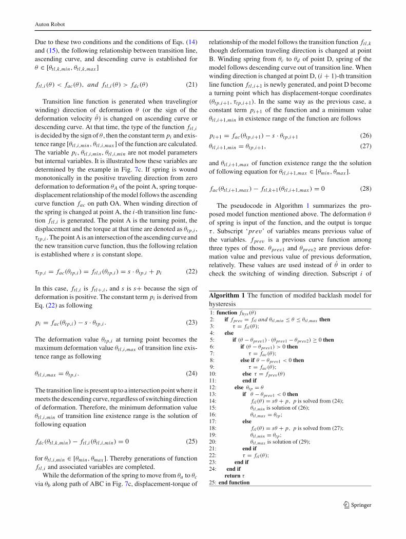
The pseudocode in Algorithm 1 summarizes the pro-posed model function mentioned above. The deformation θ
of spring is input of the function, and the output is torqueτ . Subscript ‘prev’ of variables means previous value ofthe variables. f prev is a previous curve function amongthree types of those. θprev1 and θprev2 are previous defor-mation value and previous value of previous deformation,relatively. These values are used instead of θ in order tocheck the switching of winding direction. Subscript i of
Algorithm 1 The function of modifed backlash model forhysteresis1: function fhys(θ)
2: if f prev = ftl and θtl,min ≤ θ ≤ θtl,max then3: τ = ftl (θ);4: else5: if (θ − θprev1) · (θprev1 − θprev2) ≥ 0 then6: if (θ − θprev1) > 0 then7: τ = fac(θ);8: else if θ − θprev1 < 0 then9: τ = fac(θ);10: else τ = f prev(θ)
11: end if12: else θtp = θ
13: if θ − θprev1 < 0 then14: ftl (θ) = sθ + p, p is solved from (24);15: θtl,min is solution of (26);16: θtl,max = θtp;17: else18: ftl (θ) = sθ + p, p is solved from (27);19: θtl,min = θtp;20: θtl,max is solution of (29);21: end if22: τ = ftl (θ);23: end if24: end if
return τ
25: end function
123
Auton Robot
H2
H1
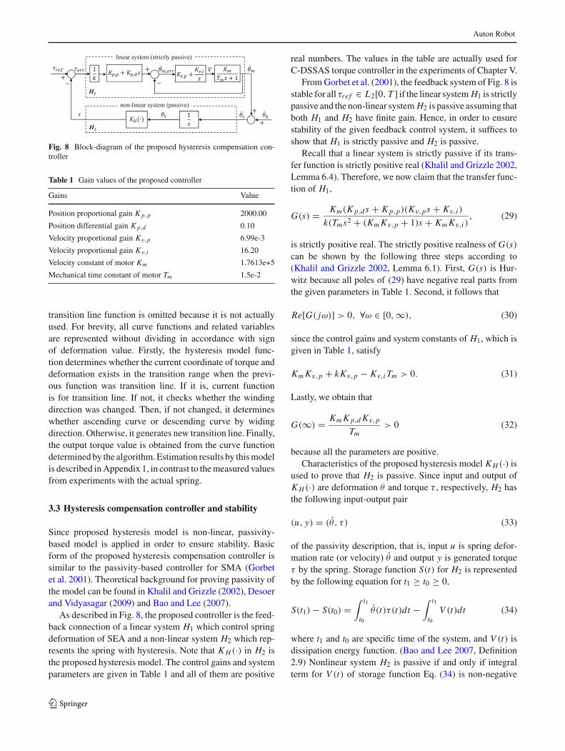
Fig. 8 Block-diagram of the proposed hysteresis compensation con-troller
Table 1 Gain values of the proposed controller
Gains Value
Position proportional gain Kp,p 2000.00
Position differential gain Kp,d 0.10
Velocity proportional gain Kv,p 6.99e-3
Velocity proportional gain Kv,i 16.20
Velocity constant of motor Km 1.7613e+5
Mechanical time constant of motor Tm 1.5e-2
transition line function is omitted because it is not actuallyused. For brevity, all curve functions and related variablesare represented without dividing in accordance with signof deformation value. Firstly, the hysteresis model func-tion determines whether the current coordinate of torque anddeformation exists in the transition range when the previ-ous function was transition line. If it is, current functionis for transition line. If not, it checks whether the windingdirection was changed. Then, if not changed, it determineswhether ascending curve or descending curve by widingdirection. Otherwise, it generates new transition line. Finally,the output torque value is obtained from the curve functiondeterminedby the algorithm.Estimation results by thismodelis described inAppendix 1, in contrast to themeasured valuesfrom experiments with the actual spring.
3.3 Hysteresis compensation controller and stability
Since proposed hysteresis model is non-linear, passivity-based model is applied in order to ensure stability. Basicform of the proposed hysteresis compensation controller issimilar to the passivity-based controller for SMA (Gorbetet al. 2001). Theoretical background for proving passivity ofthe model can be found in Khalil and Grizzle (2002), Desoerand Vidyasagar (2009) and Bao and Lee (2007).
As described in Fig. 8, the proposed controller is the feed-back connection of a linear system H1 which control springdeformation of SEA and a non-linear system H2 which rep-resents the spring with hysteresis. Note that KH (·) in H2 isthe proposed hysteresis model. The control gains and systemparameters are given in Table 1 and all of them are positive
real numbers. The values in the table are actually used forC-DSSAS torque controller in the experiments of Chapter V.
FromGorbet et al. (2001), the feedback system of Fig. 8 isstable for all τre f ∈ L2[0, T ] if the linear system H1 is strictlypassive and the non-linear system H2 is passive assuming thatboth H1 and H2 have finite gain. Hence, in order to ensurestability of the given feedback control system, it suffices toshow that H1 is strictly passive and H2 is passive.
Recall that a linear system is strictly passive if its trans-fer function is strictly positive real (Khalil and Grizzle 2002,Lemma 6.4). Therefore, we now claim that the transfer func-tion of H1,
G(s) = Km(Kp,ds + Kp,p)(Kv,ps + Kv,i )
k(Tms2 + (KmKv,p + 1)s + KmKv,i ), (29)
is strictly positive real. The strictly positive realness of G(s)can be shown by the following three steps according to(Khalil and Grizzle 2002, Lemma 6.1). First, G(s) is Hur-witz because all poles of (29) have negative real parts fromthe given parameters in Table 1. Second, it follows that
Re[G( jω)] > 0, ∀ω ∈ [0,∞), (30)
since the control gains and system constants of H1, which isgiven in Table 1, satisfy
KmKv,p + kKv,p − Kv,i Tm > 0. (31)
Lastly, we obtain that
G(∞) = KmKp,d Kv,p
Tm> 0 (32)
because all the parameters are positive.Characteristics of the proposed hysteresis model KH (·) is
used to prove that H2 is passive. Since input and output ofKH (·) are deformation θ and torque τ , respectively, H2 hasthe following input-output pair
(u, y) = (θ , τ ) (33)
of the passivity description, that is, input u is spring defor-mation rate (or velocity) θ and output y is generated torqueτ by the spring. Storage function S(t) for H2 is representedby the following equation for t1 ≥ t0 ≥ 0,
S(t1) − S(t0) =∫ t1
t0θ (t)τ (t)dt −
∫ t1
t0V (t)dt (34)
where t1 and t0 are specific time of the system, and V (t) isdissipation energy function. (Bao and Lee 2007, Definition2.9) Nonlinear system H2 is passive if and only if integralterm for V (t) of storage function Eq. (34) is non-negative
123

Auton Robot
real. (Bao andLee2007,Definitions 2.8 and2.9)The functionV (t) means the amount of energy lost by the friction fromthe elastic potential energy that was stored in the spring. Theamount of lost energy is equal to the sum of area of closedhysteresis loops. Thus, V (t) is described by the followingequation for t1 ≥ t0 ≥ 0,
∫ t1
t0V (t)dt =
n∑k=1
∮c,k
θ τdt =n∑
k=1
∮c,k
dθ
dtτdt
=n∑
k=1
∮c,k
τdθ
=p∑
k=1
∮c,k
τ+dθ +q∑
k=1
∮c,k
(−1) · τ−dθ
= sum of closed path area
≥ 0
(35)
where n is total number of closed loops, p is the numberof closed loops generated in positive deformation, q is thenumber of closed loops generated in negative deformation,τ+ is generated torque in positive deformation, and τ− isgenerated torque in negative deformation. The sum of closedloop area in proposed model is non-negative, therefore, H2
is passive. Detailed proof is given in Appendix 2.
4 Design of C-DSSAS and spiral springs
4.1 Design of C-DSSAS
The C-DSSAS is the compact version of DSSAS (Kim et al.2013) from our previous work. C-DSSAS is intended toenable a variety of experiments for rehabilitation robots,and an exoskeleton robot with C-DSSAS was developed forperforming rehabilitation exercises with wearing the robots.Figure 9 shows the developed C-DSSAS and the 1-degree-of-freedom (DOF) exoskeleton robot on the knee.
For miniaturization and weight reduction of C-DSS-AS,the overall layout was designed in the form of the accumula-tion of thin parts, and appropriate off-the-shelf componentswere selected for this purpose. The main parts, including themotor, speed reducer, and spring were modularized respec-tively to implement a variety of specifications of the SEA.Specifications of each fabricated module are described inTable 2. Figure 10 depicts three modules of C-DSSAS andits spring module. Torque transmission teeth on the input andoutput side of the inner shaft were designed as toy blocks fortorque transfer. Spiral torsion springs are used as mechanicalelastic elements and coupled to each other antagonistically bythe inner shaft and the outer arm. A 13-bit magnetic absoluteencoder for directly measuring the deflection angle of the
Fig. 9 Developed C-DSSAS, knee brace, and assembled kneeexoskeleton robot
Table 2 Specifications of C-DSSAS modules
Modules Specification
Motor Electric Synchronous AC motor
Rated torque : 2.3Nm
Rated speed : 4000RPM
Rated power : 450W
Gear Planetary Gear
Gear ratio : 25:1
Spring Magnetic Absolute Encoder
Resolution : 8192 counts/rev.
spring was installed inside the spring module. The encodersignal is passed through a specially designed connector toanother module. The left side of Fig. 9 shows a knee brace ofthe exoskeleton robot. This mechanism was designed withreference to knee braces on the market and other existingexoskeleton robots. For safety, the knee joint was designednot to bend over outside the range of 120 ◦.
4.2 Design of spiral torsion springs
To conduct the experiments, three different spiral torsionsprings were designed as per the specifications of Table 3.The design parameters are represented in Fig. 11a, and thefabricated springs are shown in Fig. 11b–d. Spring parame-ters were calculated for the desired stiffness by the followingspring formulas (Associated Spring 1981; http://mitcalc.com/doc/springs/help/en/springs.htm):
k = E · b · t312L
(36)
L = π · n · (Di + De)
2(37)
123

Auton Robot
Fig. 10 Modules of C-DSSAS. a Three modules of C-DSSAS. bExploded view of the spring modules
Table 3 Design parameters of three spiral torsion springs
Springs Parameters Value
Common Modulus of elasticity E 200 Mpa
Thickness of spring trip t 3 mm
Width of spring strip b 10 mm
Inner diameter of spring Di 18 mm
Outer diameter of spring De 71 mm
Low Number of active coils n 4.87
Stiffness of torsion spring k 6.60 Nm/rad
Medium Number of active coils n 3.90
Stiffness of torsion spring k 8.25 Nm/rad
High Number of active coils n 2.92
Stiffness of torsion spring k 11.02 Nm/rad
Equation (36) shows the relationship between the stiffnessand the spring parameters, and Eq. (37) is a formula for thefunctional spring length L in Eq. (36). There were manufac-turing errors in the design parameters of the inner diameterof the spring, outer diameter of the spring, and the number ofactive coils. The measured stiffness results are accordinglylower than the designed values. The stiffness of each springfrom linear regression of measured torque-displacement datais 4.9 Nm/rad, 6.4 Nm/rad, and 9.7 Nm/rad, respectively. Thestiffness of each spring module is 9.8 Nm/rad, 12.8 Nm/rad,
(a) (b)
(c) (d)
Fig. 11 Spiral springs for experiments. a Design parameters of spiralsprings. b Low stiffness spring. c Medium stiffness spring. d Highstiffness spring
and 19.5 Nm/rad according to Eq. (7) for an antagonisticspring connection.
5 Experiments
The controller proposed in Sect. 3 was employed in theexperiments for Sect. 2. For this reason, we firstly cover theexperiments for the hysteresis compensation controller, andthen we deal with the experiments about the torque controlperformance in accordance with the torque stiffness.
5.1 Torque control without external motion
The first experiments were conducted to test the perfor-mance of the proposed spring hysteresis compensation torquecontroller in the absence of external motion. In these experi-ments, the accuracy of the controllerswith andwithout springhysteresis model are compared. The experiments were car-ried out for three stiffness of the spring module mentioned inSect. 4.2. Prior to the experiments, the model parameters foreach spring were extracted via a model parameter identifica-tion process. The details of this procedure are described inAppendix 1. Table 4 shows the model parameters extractedfrom the process. The parameters have data on the maximumorder numbers and coefficients for polynomial functions ofascending and descending curves, and constants for the gra-dients of the transition lines.
123

Auton Robot
Table4
Parametersof
threespringsfortheproposed
hysteresismodel
f ac(
θ)or
f dc(
θ)=
a nθn
+a n
−1θn−
1+
···+a 2
θ2+
kθ,
f tl(
θ)=
sθ+
p
Low
stiffness(k=9.768Nm/rad)
Medium
stiffness(k=12.770
Nm/rad)
Highstiffness(k=19.470
Nm/rad)
na 5
a 4a 3
a 2n
a 5a 4
a 3a 2
na 7
a 6a 5
a 4a 3
a 2
f al+
5−2
.501
8.877
−10.122
4.053
5−1
0.332
27.001
−22.200
6.203
7−1
613.7
4502.2
−4798.6
2431.3
−589.9
58.4
f al+
52.021
6.967
8.854
4.483
50.440
1.188
4.019
3.525
7−1
071.2
−2486.2
−1997.3
−620.1
−47.5
4.2
f al+
52.438
−8.305
9.946
−4.651
5−0
.636
17.379
−12.726
1.685
7−1
322.3
3321.9
−3045.7
1239.9
−219.3
14.3
f al+
5−4
.106
−15.589
−19.281
−8.231
5−7
.19
−20.014
−17.080
−4.751
7−1
225.6
−3250.3
−3260.6
−1554.1
−364.8
−37.142
ss +
=12
.551
,s −
=13
.176
s +=
18.977
,s −
=21
.211
s +=
28.332
,s −
=25
.464
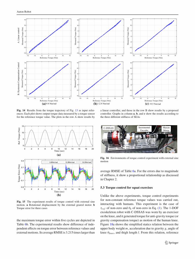
Figure 12 depicts the experimental setup for implementingthe proposed torque controller in Fig. 8. A microcon-troller (NUCLEO-F446RE, STM32)with a 180-MHzCPU isexpoited as a main operational unit for the torque controller.It has the proposed hysteresis model and a position con-troller for spring deformation control. The microcontrolleris connected with a servo drives (DC Whistle, Elmo) of ageared motor in cascade. The analog voltage signal fromthe microcontroller is inputted to the servo driver, and thenthe integrated velocity from the geared motor is outputted.The integrated deformation velocity of spring by the gearedmotor and external motion is inputted to the microcontrollerthrough an absolute magnetic encoder (RMB28SC, RLS)with a 13-bit resolution per revolution. Note that there isno external movement in experiments of this sub-chapter.The reference torque trajectory shown in Fig. 13 is transmit-ted from theCompact-RIO to themicrocontroller byRS-232.TheC-DSSAS as an SEAgenerates torque by the torque con-troller, and a torque sensor (TCN-10K, Dacell) connected inseries with C-DSSAS reads the physical torque value. Thespring block of Fig. 12 has the proposed hysteresis modelin the case of the hysteresis compensation torque controller,or this block has linear stiffness values obtained by linearregression in the case of the linear torque controller. Gainsfor the controller were set as described in Table 1 regardlessof the spring stiffness, and values of the gains satisfy the con-ditions for passivity described in Sect. 3.3. Figure 12 showsthe experimental results with plots of reference torque andmeasured output torque data. Plots in rowA show the case ofthe linear controller, and those of row B show the case of thehysteresis compensation controller. Graphs that are closer tolinear imply more accurate torque output. It can be shownthat the results of row B are more linear than the results ofrow A. For quantitative confirmation, we calculated the non-linearity error (Kuhnen 2003) of torque control defined by
max1≤t≤te
{∣∣τre f (t)) − τ(t)∣∣}
max1≤t≤te
{∣∣τre f (t)∣∣} (38)
where t is time, te is the end of the experiment time, τre f (t)is the reference torque data at that time, and τ(t) is themeasured torque data at that time. Non-linearity error val-ues are described in Table 5 corresponding to each springand controller. This result shows that the proposed hystere-sis compensation torque controllers generate more accuratetorque output (Fig. 14).
An additional experiment for torque control in the absenceof external motion was conducted to contrast with the exper-iments to be performed on the following two subchapters. Itis the case of τre f of non-zero and θh of zero in Eq. (1). In thisexperiment, we observed torque errors when desired torquevalues were given as a sine wave that has a period of 4 s
123

Auton Robot
Fig. 12 Experiment setup forproposed torque controller
0 20 40 60 80 100 120Time (sec)
-15
-10
-5
0
5
10
15
Ref
eren
ce T
orqu
e (N
m)
Fig. 13 Reference torque trajetory for the experiments
Table 5 Non-linearity torque control error of linear controller and hys-teresis compensation controller
Controller Non-linearity error(%)
Spring stiffness (Nm/rad) Average
9.8 12.8 19.5
Linear 7.786 6.214 7.643 7.214
Hysteresis 4.250 3.786 3.929 3.988
as shown in Fig. 15a. Though testing for various bandwidthis desireable, we carried out the experiments in sufficientlylow bandwidth in order to reduce effects due to the specifica-tions of a geared motor in SEA. Figure 15b shows the torqueerrors between reference values and torque values estimatedby proposed hysteresis model in the controller. As describedin Chapter 2 , there should be no difference of the torque errorbetween the three cases. However, the plot shows that theSEA of lower stiffness has lower error though its differenceis smaller than results of experiments in next two subchap-ters. It is presumed due to resolution as mentioned in Chapter2, but it requires further analysis in our future works. For
quantitative comparison, the root mean squre error (RMSE)is obtained from data within five cycles, and its results aretabulated in Result (a) of Table 6.
5.2 Torque control with external sine motion
In this experiment, the torque controllers of SEAs with dif-ferent stiffnesses are examined in the condition that desiredtorque is zero, while outside of SEA is interacted with a cer-tain motion. This experiment means the case of τre f of zeroand θh of non-zero in Eq. (1). Figure 16 shows the experi-mental setup. A geared motor (DC motor, Maxon) and servodrives (EPOS2 70/10, Maxon) were used in order to imple-ment regular external motion. The geared motor has a powerof 150 W, maximum no-load speed of 7580 RPM, and max-imum torque of 40.7 Nm with a reduction gear of 230:1. Aservo drive of 700 W was exploited for position control ofthe motor. The motor was connected directly to C-DSSASfor applying forcedmovements by position control. A hollowincremental encoder (E40-H-8-5000, Autonics) was used tomeasure the external displacement by the motor. Controlgains were the same as shown in Table 1 regardless of thespring stiffness, and only the spring module of C-DSSASwas changed.
When a constant reference torque of zero is inputted tothe proposed controller, the geared motor moves with a sinu-soidal position trajectory with an amplitude of 45 ◦ and aperiod of 4 s, as shown in Fig. 17a. We measured the torqueerror through the torque value estimated by the hysteresismodel and external displacement by the encoder. The resultsof the measured data according to the time are depicted inFig. 17b. A smaller torque error is exhibited for the lowerstiffness of the spring in the plots. Results for the RMSE and
123
Auton Robot
-15 -10 -5 0 5 10 15
Reference Torque (Nm)
-15
-10
-5
0
5
10
15
Mea
sure
d T
orqu
e (N
m)
-15 -10 -5 0 5 10 15
Reference Torque (Nm)
-15
-10
-5
0
5
10
15
Mea
sure
d T
orqu
e (N
m)
-15 -10 -5 0 5 10 15
Reference Torque (Nm)
-15
-10
-5
0
5
10
15
Mea
sure
d T
orqu
e (N
m)
-15 -10 -5 0 5 10 15
Reference Torque (Nm)
-15
-10
-5
0
5
10
15
Mea
sure
d T
orqu
e (N
m)
-15 -10 -5 0 5 10 15
Reference Torque (Nm)
-15
-10
-5
0
5
10
15
Mea
sure
d T
orqu
e (N
m)
-15 -10 -5 0 5 10 15
Reference Torque (Nm)
-15
-10
-5
0
5
10
15
Mea
sure
d T
orqu
e (N
m)
(a) (b) (c)
Fig. 14 Results from the torque trajectory of Fig. 13 as input refer-ences: Each plot shows output torque data measured by a torque sensorfor the reference torque value. The plots in the row A show results by
a linear controller, and those in the row B show results by a proposedcontroller. Graphs in column a, b, and c show the results according tothe three different stiffness of SEAs
0 2 4 6 8 10 12 14 16 18 20
Time (sec)
-0.2
-0.1
0
0.1
0.2
Tor
que
Err
or (
Nm
)
9.8Nm/rad 12.8Nm/rad 19.5Nm/rad
0 2 4 6 8 10 12 14 16 18 20
Time (sec)
0
5
10
15
Ref
. Tor
que
(Nm
)
(a)
(b)
Fig. 15 The experiment results of torque contorl with external sinemotion. a Rotational displacement by the external geared motor. bTorque error for three cases
the maximum torque error within five cycles are depicted inTable 6b. The experimental results show difference of inde-pendent effects on torque error between reference values andexternalmotions. Its averageRMSE is 3.215 times larger than
Fig. 16 Environments of torque control experiment with external sinemotion
average RMSE of Table 6a. For the errors due to magnitudeof stiffness, it show a proportional relationship as discussedin Chapter 2.
5.3 Torque control for squat exercises
Unlike the above experiments, torque control experimentsfor non-constant reference torque values was carried out,interacting with humans. This experiment is the case ofτre f of non-zero and θh of non-zero in Eq. (1). The 1-DOFexoskeleton robot with C-DSSAS was worn by an exerciseron the knee, and it generated torque for anti-gravity torque (orgravity compensation torque) as motion of the human knee.Figure 18a shows the simplified statics relation between theupper body weight m, acceleration due to gravity g, angle ofknee θknee, and thigh length l. From this relation, reference
123

Auton Robot
0 2 4 6 8 10 12 14 16 18 20
Time (sec)
-0.4
-0.2
0
0.2
0.4
0.6
Tor
que
Err
or (
Nm
)
9.8Nm/rad 12.8Nm/rad 19.5Nm/rad
0 2 4 6 8 10 12 14 16 18 20
Time (sec)
-50
0
509.8Nm/rad 12.8Nm/rad 19.5Nm/rad
(a)
(b)
Fig. 17 The experiment results of torque contorl with external sinemotion. a Rotational displacement by the external geared motor. bTorque error for three cases
torque τre f for anti-gravity is calculated by
τre f = τanti−g = −r · τg
= −r · lmg · sin(
π − θknee
2
)
= −α · sin(
π − θknee
2
) (39)
where τanti−g is the assist torque for anti-gravity, τg is thetorque due to gravity, r is the assist ratio, and a is a constantfor the experiment. The constant α was set to obtain a similartrajectory with the second test in Chapter 5.1. The range ofθknee is approximately 0 to 90 degree, similar to the experi-ments of the Chapter 5.2. A repetition period of exercise is4 second in common with other experiments. The exerciserchecked a stopwatch continuously and shouted a number inorder to maintain the time intervals. As with other experi-ments, the control gain followed Table 1, and only the springmodules were replaced during the experiments.
(a) (b)
Fig. 18 Squat exercise experiments. a Simplified statics relation insquat exercise. b Squat exercise wearing the exoskeleton robot withC-DSSAS
Figure 19a–c represents the generated reference torque byEq. ( 39) and generated output torque by C-DSSAS depend-ing on stiffness. The output torque value is estimated bythe proposed static hysteresis model. Figure 19d shows thetorque error between the reference and the output. This graphshows that the SEA of lower stiffness has lower torque error,as with results of Chapter 5.2. Table 6c desribes RMSE andmaximum error of this results. The RMSEs of this experi-ment is larger than the results in Table 6a, but it is lowerthan the results in Table 6b. Since, in this experiment, thehuman motion assists the SEA to reach desired torque valuebecause the direction of rotation by human is different fromthose of rotation by a geared motor of SEA for generatingtorque are different. This corresponds to the case that τre f hasopposite sign from θh in Eq. (1), thus the absolute magnitudeof the error is reduced. The relationship between force andmovement in this case can also be occurred in other robots foractive exercise. Besides the case in this experiment, for exam-ple, the strength exercises such as leg extension have a samecharacteristic. Even though the error is reduced for this rea-son, the torque error due to the spring stiffness still remains.Accordingly, the spring stiffness is left as an important fac-tor of the torque error. After all, the low stiffness reduces thetorque error, and this conclusion can be confirmed from theresult of Table 6c. It also means that the low stiffness con-tributes to robust torque control and reduction of interactiontorque between robot and human.
Table 6 Root mean square torque error (RMSE) and maximum torqueerror of experimental results: (a) Torque control for non-zero referencevalue without external motion (b) Torque control for zero reference
value with regular external motion by a geared motor (c) Torque controlfor non-zero reference value with external motion by a human exerciser
Stiffness (a) (b) (c)
(Nm/rad) RMSE (Nm) Max. Error (Nm) RMSE (Nm) Max. Error (Nm) RMSE (Nm) Max. Error (Nm)
9.8 0.0429 0.1042 0.1293 0.2192 0.1133 0.2743
12.8 0.0556 0.1238 0.1591 0.2465 0.1364 0.3001
19.5 0.0728 0.1786 0.2623 0.4407 0.2203 0.4799
123

Auton Robot
0 2 4 6 8 10 12 14 16 18 20
Time (sec)
0
10
20T
orqu
e (N
m)
Reference torque Estimated torque
0 2 4 6 8 10 12 14 16 18 20
Time (sec)
0
10
20
Tor
que
(Nm
)
Reference torque Estimated torque
0 2 4 6 8 10 12 14 16 18 20
Time (sec)
0
10
20
Tor
que
(Nm
)
Reference torque Estimated torque
0 2 4 6 8 10 12 14 16 18 20
Time (sec)
-0.5
0
0.5
1
Err
or (
Nm
) 9.8Nm/rad 12.8Nm/rad 19.5Nm/rad
(a)
(b)
(c)
(d)
Fig. 19 Result of the squat experiment. a Reference and estimatedoutput torque of 9.8 Nm/rad stiffness spring module. b Reference andestimated output torque of 12.8 Nm/rad stiffness spring module. c Ref-erence and estimated output torque of 19.5 Nm/rad stiffness springmodule. d Torque errors for each spring module
6 Conclusion and discussion
Active exercises are general exercises in which the exerciserscontrol their body themselves, such as strength exercises andaerobic exercises. Robots for active exercises can be appliedfor providing proper load conditions for safe and proper exer-cises. Weight support robots and strength training robots areproper examples of rehabilitation robots for active exercises.The final output of these robots is force or torque,whereas thefinal outputs of existing robots for passive or active-assistiverehabilitation exercises are position or impedance. Therefore,SEAs for active exercise robots are required high quality oftorque (or force) control. In this paper, a low-stiffness designis proposed for robust and high-resolution torque control,and a hysteresis compensation controller is introduced forhigh-accuracy torque control.
A low-stiffness SEA design for robust control is describedby theoretical considerations with a linear torque controller,and results of experiments demonstrate those. The lower stiff-ness of the SEA reduces the influence of external humanmotion and improves the torque resolution of the SEA in thepractical design. Experiments were conducted with lowertorque and stiffness than existing SEAs, but the same effectsof the low-stiffness design are expectedwhen it applied to theactual robot rehabilitationwith sufficient torque and stiffness.
However, further studies are needed in order to optimal stiff-ness design of SEA for active exercise robots. In the future,we will conduct further studies on how to obtain optimumstiffness of the robot designwith specific active rehabilitationexercises.
A hysteresis compensation torque controller for accu-racy control is proposed with a polynomial-based modifiedbacklash model and passivity-based control, and relatedexperiments were conducted by measuring its non-linearityerror. The proposedmodel is effective formechanical springswhich have thin hysteresis and antagonistic connection, butthe model have limitations for describing complex hystere-sis loops. Therefore, we need to develop an improved modelthat can depict the complex hysteresis of springs in order toachieve high accuracy. In addition, comparative studies areneeded on the hysteresis characteristics between springs andother materials and onmodel accuracy between the proposedand existing models.
Acknowledgments This work have been supported by the NationalResearch Foundation of Korea funded by the Ministry of Science, ICTand Future Planning (2011-0011341 and 2015-055375).
Appenndix 1: Model parameter identification
The model parameters are calculated from torque data forthe deformation of the spring obtained by the experimentswith actual springs. First, the parameters associated with theascending curve and the descending curve are firstly cal-culated from data of blue solid lines as shown in Fig. 20bwhen spring deformation trajectory is given from blue solidlines in Fig. 20a. These data is the experimental data for themedium stiffness spring of Table 4. The trajectory shuttlewith a constant speed between the minimum and maximumvalue of predetermined deformation range. Although a per-missible torque range of the SEA was about 14 Nm torquespring, we set the deformation range for spring identificationabout 16 Nm with marginal range. First, the linear stiffnessk is obtained by the linear regression from the total data assatisfying following format
τ = kθ. (40)
Then data is classified into four of positive ascending curve,negative ascending curve, positive descending curve, andnegative descending curve, based on the sign of displace-ment and its velocity. Specific parts of data speculated totransition line are removed discretionally. We discarded apart of data as much as 0.05rad frommaximum displacementof positive descending curve and minimum deformation ofnegative ascending curve. The four curve functions of themodel are obtained through polynomial regression processthat meets the format of Eq. (17). We decided properdegrees of the polynomials though trial and error, and
123
Auton Robot
-1 -0.5 0 0.5 1
Deformation(rad)
-15
-10
-5
0
5
10
15
Torq
ue(N
m)
0 50 100 150 200 250 300 350 400 450 500
Time(sec)
-1
0
1R
ef
De
form
atio
n(r
ad
)
(a)
(b)
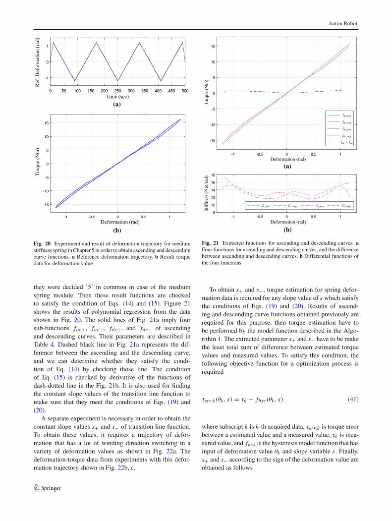
Fig. 20 Experiment and result of deformation trajectory for mediumstiffness spring inChapter 5 in order to obtain ascending and descendingcurve functions. a Reference deformation trajectory. b Result torquedata for deformation value
they were decided ’5’ in common in case of the mediumspring module. Then these result functions are checkedto satisfy the condition of Eqs. (14) and (15). Figure 21shows the results of polynomial regression from the datashown in Fig. 20. The solid lines of Fig. 21a imply foursub-functions fac+, fac−, fdc+, and fdc− of ascendingand descending curves. Their parameters are described inTable 4. Dashed black line in Fig. 21a represents the dif-ference between the ascending and the descending curve,and we can determine whether they satisfy the condi-tion of Eq. (14) by checking those line. The conditionof Eq. (15) is checked by derivative of the functions ofdash-dotted line in the Fig. 21b. It is also used for findingthe constant slope values of the transition line function tomake sure that they meet the conditions of Eqs. (19) and(20).
A separate experiment is necessary in order to obtain theconstant slope values s+ and s− of transition line function.To obtain these values, it requires a trajectory of defor-mation that has a lot of winding direction switching in avariety of deformation values as shown in Fig. 22a. Thedeformation-torque data from experiments with this defor-mation trajectory shown in Fig. 22b, c.
-1 -0.5 0 0.5 1
Deformation(rad)
-15
-10
-5
0
5
10
15
Tor
que(
Nm
)
fac,pos
fac,neg
fdc,pos
fdc,neg
fac- f
dc
-1 -0.5 0 0.5 1
Deformation(rad)
8
10
12
14
16
18
Stif
fnes
s(N
m/r
ad)
fac,pos
fac,neg
fdc,pos
fdc,neg
(a)
(b)
Fig. 21 Extracted functions for ascending and descending curves. aFour functions for ascending and descending curves, and the differencebetween ascending and descending curves. b Differential functions ofthe four functions
To obtain s+ and s−, torque estimation for spring defor-mation data is required for any slope value of s which satisfythe conditions of Eqs. (19) and (20). Results of ascend-ing and descending curve functions obtained previously arerequired for this purpose, then torque estimation have tobe performed by the model function described in the Algo-rithm 1. The extracted parameter s+ and s− have to be makethe least total sum of difference between estimated torquevalues and measured values. To satisfy this condition, thefollowing objective function for a optimization process isrequired
τerr,k(θk, s) = τk − fhys(θk, s) (41)
where subscript k is k-th acquired data, τerr,k is torque errorbetween a estimated value and a measured value, τk is mea-sured value, and fhys is the hysteresismodel function that hasinput of deformation value θk and slope variable s. Finally,s+ and s− according to the sign of the deformation value areobtained as follows
123

Auton Robot
-1 -0.5 0 0.5 1
Deformation(rad)
-15
-10
-5
0
5
10
15
Torq
ue(N
m)
-1 -0.5 0 0.5 1
Deformation(rad)
-15
-10
-5
0
5
10
15
Torq
ue(N
m)
-1 -0.5 0 0.5 1
Deformation(rad)
-15
-10
-5
0
5
10
15
Torq
ue(N
m)
-1 -0.5 0 0.5 1
Deformation(rad)
-15
-10
-5
0
5
10
15
Torq
ue(N
m)
0 200 400 600 800 1000 1200 1400 1600
Time(sec)
-1
-0.5
0
0.5
1R
ef D
efor
mat
ion(
rad)
(a)
(b) (d)
(c) (e)
Fig. 22 Experiment and results for extracting slope constants of tran-sition line. a Deformation trajectory. b Measured data for the greenpart of the trajectory. c Measured data for the blue and red part. d Esti-
mated data by obtained slope constant values for the green part of thetrajectory. e Estimated data for the blue and red part
s+ = argmins∈(s+,min ,∞)
n∑k=1
τerr,k,+(θk, s) (θk ≥ 0) (42)
s− = argmins∈(s−,max ,∞)
n∑k=1
τerr,k,−(θk, s) (θk < 0) (43)
where s+,min and s,min are from the conditions of Eqs. (19)and (20). In thismanner, all of the parameters of the proposedmodel are obtained. Table 7 describes torque error betweenestimation value andmeasured value of the springs accordingto models.
123
Auton Robot
Table 7 Error between measured torque value and estmatied value byspring models for the three springs
Model Error Stiffness (Nm/rad)
9.8 12.8 19.5
Linear RMSE (Nm) 0.385 0.271 0.312
Max. Error (Nm) 1.042 1.132 0.998
Hysteresis RMSE (Nm) 0.115 0.087 0.089
Max. Error (Nm) 0.646 0.527 0.584
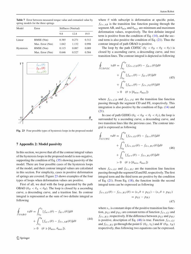
Fig. 23 Four possible types of hysteresis loops in the proposed model
7 Appendix 2: Model passivity
In this section, we prove that all of the contour integral valuesof the hysteresis loops in the proposedmodel is non-negative,supporting the condition of Eq. (35) showing passivity of themodel. There are four possible cases of the hysteresis loopsof the model, and their contour integral values are calculatedin this section. For simplicity, cases in positive deformationof springs are covered. Figure 23 shows examples of the fourtypes of loops when deformation values are positive.
First of all, we deal with the loop generated by the pathOBAO (θO < θA < θB). The loop is closed by a ascendingcurve, a descending curve, and a trasition line. Its contourintegral is represented as the sum of two definite integral asfollowing
∮OABO
τdθ =∫ θA
θO
[ fac+(θ) − fdc+(θ)]dθ
+∫ θB
θA
[ fac+(θ) − ftl+,AB(θ)]dθ
> 0 (θ [θmin, θmax ]).
(44)
where θ with subscript is deformation at specific point,ftl+,AB is the transition line function passing through thesegment AB, and θmin and θmax are minimum and maximumdeformation values, respectively. The first definite integralterm is positive from the condition of Eq. (14), and the sec-ond term is also positive the condition of Eq. (21). Thus thecontour integral of path OBAO is positive.
The loop by the path CDFEC (θC < θD < θE < θF ) isclosed by a ascending curve, a descending curve, and twotransition lines. The contour integral is depicted as following
∮CDFEC
τdθ =∫ θD
θC
[ ftl+,CD(θ) − fdc+(θ)]dθ
+∫ θE
θD
[ fac+(θ) − fdc+(θ)]dθ
+∫ θF
θE
[ fac+(θ) − ftl+,FE (θ)]dθ
> 0 (θ [θmin, θmax ])
(45)
where ftl+,CD and ftl+,FE are the transition line functionpassing through the segment CD and FE, respectively. Thisintegration is also positive by the condition of Eqs. (14) and(21).
In case of path GIJHG (θG < θH < θI < θJ ), the loop issurrounded by a ascending curve, a descending curve, andtwo transition lines like the previous case. The contour inte-gral is expressed as following∮GI J HG
τdθ =∫ θH
θG
[ ftl+,GI (θ) − fdc+(θ)]dθ
+∫ θI
θH
[ ftl+,GI (θ) − ftl+,H J (θ)]dθ
+∫ θJ
θI
[ fac+(θ) − ftl+,H J (θ)]dθ
> 0 (θ [θmin, θmax ])
(46)
where ftl+,GI and ftl+,H J are the transition line functionpassing through the segmentGI andHJ, respectively. Thefirstintegral term and the third term are positive by the conditionof Eq. (21). From Eq. (18), the function inside the secondintegral term can be expressed as following
ftl+,GI (θ) − ftl+,H J (θ) = (s+θ + pGI ) − (s+θ + pH J )
= pGI − pH J
(47)
where s+ is constant slope of the positive transition line func-tion, pGI and pH J are constant terms of function ftl+,GI andftl+,H J , respectively. If the difference between pGI and pH J
is positive, description of Eq. (46) is true. Function ftl+,GI
and ftl+,H J go through the pointG (θG, τG) and H (θH , τH )
respectively, thus following two equations can be expressed.
123

Auton Robot
{τG = s+θG + pGI
τH = s+θH + pH J(48)
By simplifying Eq. (48) for constants pGI and pH J and thensubstituting these equations to Eq. (47), following result isobtained from the condition of Eq. (21).
pGI − pH J = s+(θH − θG) − (τH − τG)
= ftl+,GI (θH ) − ftl+,GI (θG)
θH − θG· (θH − θG)
− ( fdc+(θH ) − fdc+(θG))
= ftl+,GI (θH ) − fdc+(θH )
> 0 (θ [θmin, θmax ])(49)
Therefore, description of Eq. (46) is true.The path KLK(θK < θL ) is only on a transition line, thus
there is no hysteresis loop by the model. The contour integralof this case is represent as following
∮K LK
τdθ =∫ θL
θK
[ ftl+,K L(θ) − ftl+,K L(θ)]dθ
= 0 (θ [θmin, θmax ])(50)
where ftl+,K L is the transition line function passing throughthe segment KL.
References
Akdogan, E., & Adli, M. A. (2011). The design and control of a thera-peutic exercise robot for lower limb rehabilitation: Physiotherabot.Mechatronics, 21(3), 509–522.
Andrews, J. R.,Harrelson,G. L.,&Wilk,K. E. (2011).Physical rehabil-itation of the injured athlete. Philadelphia, PA: Elsevier Saunders.
Associated Spring. (1981) Design handbook: Engineering guide tospring design. Associated Spring, Barnes Group Inc.
Au, S. K., Herr, H., Weber, J., Martinez-Villalpando, E. C. (2007).Powered ankle-foot prosthesis for the improvement of amputeeambulation. Engineering in Medicine and Biology Society, 2007.EMBS 2007. 29th Annual International Conference of the IEEE,(pp. 3020–3026), IEEE.
Bao, J., & Lee, P. L. (2007). Process control: The passive systemsapproach. Berlin: Springer Science & Business Media.
Bashash, S., & Jalili, N. (2008). A polynomial-based linear mappingstrategy for feedforward compensation of hysteresis in piezoelec-tric actuators. Journal of Dynamic Systems, Measurement, andControl, 130(3), 031008.
Colombo, G., Joerg, M., Schreier, R., & Dietz, V. (2000). Treadmilltraining of paraplegic patients using a robotic orthosis. Journal ofrehabilitation research and development, 37(6), 693.
Desoer, C. A., & Vidyasagar, M. (2009). Feedback systems: Input-output properties (Vol. 55). Philadelphia, PA: SIAM.
Díaz, I., Gil, J. J., Sánchez, E. (2011). Lower-limb robotic rehabilita-tion: Literature review and challenges. Journal of Robotics, 2011,759764. doi:10.1155/2011/759764.
Foliente, G. C. (1995). Hysteresis modeling of wood joints andstructural systems. Journal of Structural Engineering, 121(6),1013–1022.
Freivogel, S., Mehrholz, J., Husak-Sotomayor, T., & Schmalohr, D.(2008). Gait training with the newly developed lokohelp-system isfeasible for non-ambulatory patients after stroke, spinal cord andbrain injury. a feasibility study. Brain Injury, 22(7–8), 625–632.
Frey,M.,Colombo,G.,Vaglio,M.,Bucher, R., Jorg,Matthias,&Riener,Robert. (2006). A novel mechatronic body weight support system.Neural Systems and Rehabilitation Engineering, IEEE Transac-tions on, 14(3), 311–321.
Ge, P., & Jouaneh, M. (1995). Modeling hysteresis in piezoceramicactuators. Precision Engineering, 17(3), 211–221.
Goffer, A. (2006) Gait-locomotor apparatus, December 26 2006. USPatent 7,153,242.
Gorbet, R. B., Morris, K. A., & Wang, D. W. L. (2001). Passivity-based stability and control of hysteresis in smart actuators.ControlSystems Technology, IEEE Transactions on, 9(1), 5–16.
Ham, Rv, Sugar, T. G., Vanderborght, B., Hollander, K. W., & Lefeber,D. (2009). Compliant actuator designs. Robotics & AutomationMagazine, IEEE, 16(3), 81–94.
Hesse, S., Uhlenbrock, D., et al. (2000). A mechanized gait trainer forrestoration of gait. Journal of rehabilitation research and devel-opment, 37(6), 701–708.
http://mitcalc.com/doc/springs/help/en/springs.htm. Accessed 21 June2016.
http://www.alterg.com/. Accessed 21 June 2016.http://www.aretechllc.com/. Accessed 21 June 2016.http://www.biodex.com/physical-medicine/products/dynamometers/
system-4-pro. Accessed 21 June 2016.Ikhouane, F., & Rodellar, J. (2007). Systems with hysteresis: Analysis,
identification and control using the Bouc-Wen model. Hoboken:Wiley.
Jafari, A., Tsagarakis, N. G., Vanderborght, B., Caldwell, D. G. (2010).A novel actuator with adjustable stiffness (awas). IntelligentRobots and Systems (IROS), 2010 IEEE/RSJ International Con-ference on, (pp. 4201–4206), IEEE.
Karavas, N. C., Tsagarakis, N.G., Caldwell, D.G. (2012). Design,mod-eling and control of a series elastic actuator for an assistive kneeexoskeleton. Biomedical Robotics and Biomechatronics (BioRob),2012 4th IEEE RAS & EMBS International Conference on, (pp.1813–1819), IEEE.
Khalil, H. K., & Grizzle, J. (2002). Nonlinear systems, vol. 3. UpperSaddle River: Prentice Hall.
Kim, Y., Lee, J., & Park, J. (2013). Compliant joint actuator with dualspiral springs.Mechatronics, IEEE/ASME Transactions on, 18(6),1839–1844.
Kong, K., Bae, J., & Tomizuka, M. (2009). Control of rotary serieselastic actuator for ideal force-mode actuation in human-robotinteraction applications.Mechatronics, IEEE/ASME Transactionson, 14(1), 105–118.
Kuhnen, K. (2003). Modeling, identification and compensation ofcomplex hysteretic nonlinearities: A modified prandtl-ishlinskiiapproach. European journal of control, 9(4), 407–418.
Kuhnen, K., & Janocha, H. (2001). Inverse feedforward controller forcomplex hysteretic nonlinearities in smart-material systems. Con-trol and Intelligent systems, 29(3), 74–83.
Laffranchi, M., Tsagarakis, N. G., Cannella, F., Caldwell, D. G. (2009).Antagonistic and series elastic actuators: a comparative analysison the energy consumption. Intelligent Robots and Systems, 2009.IROS 2009. IEEE/RSJ International Conference on, (pp. 5678–5684), IEEE.
Lagoda, C., Schou, A. C., Stienen, A. H. A., Hekman, E. E. G., van derKooij, H. (2010). Design of an electric series elastic actuated jointfor robotic gait rehabilitation training. Biomedical Robotics and
123

Auton Robot
Biomechatronics (BioRob), 2010 3rd IEEE RAS and EMBS Inter-national Conference on, (pp. 21–26), IEEE.
Ok, J. K., Yoo, W. S., & Sohn, J. H. (2008). New nonlinear bushingmodel for general excitations using bouc-wen hysteretic model.International Journal of Automotive Technology, 9(2), 183–190.
Pratt, J. E., Krupp, B. T., Morse, C. J., Collins, S. H. (2004). Theroboknee: An exoskeleton for enhancing strength and enduranceduring walking. Robotics and Automation, 2004. Proceedings.ICRA’04. 2004 IEEE International Conference on, (Vol 3, pp.2430–2435) , IEEE.
Rouse, E. J., Mooney, L. M., Martinez-Villalpando, E. C., Herr, H. M.(2013). Clutchable series-elastic actuator: Design of a robotic kneeprosthesis for minimum energy consumption. In RehabilitationRobotics (ICORR), 2013 IEEE International Conference on, (pp.1–6), IEEE.
Schmidt, H. (2004). Hapticwalker-a novel haptic device for walkingsimulation, Proc. of’EuroHaptics.
Sergi, F., Accoto, D., Carpino, G., Tagliamonte, N. L., Guglielmelli,E. (2012). Design and characterization of a compact rotary serieselastic actuator for knee assistance during overground walking.Biomedical Robotics and Biomechatronics (BioRob), 2012 4thIEEE RAS & EMBS International Conference on, (pp. 1931–1936), IEEE.
Veneman, J. F., Ekkelenkamp,R.,Kruidhof,R., van derHelm, F.C.T.,&van derKooij, Herman. (2006). A series elastic-and bowden-cable-based actuation system for use as torque actuator in exoskeleton-type robots. The international journal of robotics research, 25(3),261–281.
Veneman, J. F., Kruidhof, R., Hekman, E. E. G., Ekkelenkamp, R.,Van Asseldonk, Edwin H F, & Van Der Kooij, Herman. (2007).Design and evaluation of the lopes exoskeleton robot for interactivegait rehabilitation. Neural Systems and Rehabilitation Engineer-ing, IEEE Transactions on, 15(3), 379–386.
Voight, M., Hoogenboom, B., & Prentice, W. (2006). Musculoskele-tal interventions: Techniques for therapeutic exercise. New York:McGraw Hill Professional.
Wang, C.-H., Foliente, G. C., Sivaselvan, M. V., & Reinhorn, A. M.(2001). Hysteretic models for deteriorating inelastic structures.Journal of Engineering Mechanics, 127(11), 1200–1202.
West, R Gary. Powered gait orthosis and method of utilizing same,February 10 2004. US Patent 6,689,075.
Wonje Choi received the B.S.in aerospace engineering fromSeoulNationalUniversity,Korea,in 2010 and the M.S. degrees inDepartment of TransdisciplinaryStudies, Seoul Nation Universityin 2013. He is doctoral candi-date at Seoul Nation Universityin Korea.
JongseokWon received the B.S.and M.S. degrees in Mechani-cal Engineering from SoongsilUniversity, Seoul, Korea, in 1993and 1995, respectively. He iscurrently working toward thePh.D degree in the Depart-ment of Transdisciplinary Stud-ies, Seoul National University,Seoul, Korea. From 2007 to2013, he was a researcher/teammanager in Meerecompany Inc.,Korea, where he was involvedwith surgical robotics.
JiminLee received aB.S. inBio-medical engineering and Electri-cal engineering from the kyunghee university in 2012. He iscurrently PhD course studentat Seoul National University inSouth Korea.
Jaeheung Park received theB.S. and M.S. degrees in aerospace engineering from SeoulNational University, Korea, in1995 and 1999, respectively, andthe PhD degree in aeronau-tics and astronautics from Stan-ford University, U.S. in 2006.From 2006 to 2009, He wasa post-doctoral researcher andlater a research associate at Stan-ford Artificial Intelligence Lab-oratory. From 2007 to 2008,he worked part-time at HansenMedical Inc., a medical robot-
ics company in U.S. Since 2009, he has been an assistant professorin the Graduate School of Convergence Science & Technology atSeoul National University, Korea. His research interests lie in the areasof robot-environment interaction, contact force control, robust hapticteleoperation, multicontact control, whole-body dynamic control, bio-mechanics, and medical robotics.
123