Embed Size (px)
Citation preview

Software Reliability
Lou Gullo
Jon Peterson
Raytheon Company

2011 RAMS – Tutorial 12A – Gullo and Peterson 2
Topics of Discussion� Introduction
� Software Reliability Process
� Capability Maturity Model (Keene Model)
� Rayleigh Model Analysis
� Software Error Estimation Program (SWEEP)
� Computer Aided Software Reliability Estimation
� Business Case Study
� Incorporating Software Reliability Into System Ao Modeling
� Limitations
� Conclusions

2011 RAMS – Tutorial 12A – Gullo and Peterson 3
Goals
To train reliability engineers, software design engineers, software safety engineers, and system engineers in the processes and tools to find more design weaknesses and improve the Design for Software Reliability in a manner such that :
1. Mission stopping failures are minimized or reduced over the anticipated life
2. Minimize or reduce unscheduled downtime
3. Zero net cost, and the ROI must be more than the DfSR investment.

2011 RAMS – Tutorial 12A – Gullo and Peterson 4
Software Reliability Introduction
� Software reliability is the result of a reliability process
such that the s/w will perform adequately for the
period of time intended under the operating
conditions encountered……Probability of Success
� Reliability depends on the design – Must change
design to improve it
2011 RAMS – Tutorial 12A – Gullo and Peterson 5
Software Reliability Introduction
� Software has a unique feature difference compared to hardware:
Variability code to code is virtually zero (exception is upgraded codes). If the code has an error in one copy, then all copies have the error
Defects in the code are typically failures in understanding operational requirements rather than degradation of the code
x x x x xx

2011 RAMS – Tutorial 12A – Gullo and Peterson 6
Reliability in Design
How Do I Make Reliability Important in Design ?
• Collect and Analyze Data
• Determine Uncertainties and Weaknesses
• Calculate Probabilities
• Understand the Risks
• Develop Solutions with Contingencies

2011 RAMS – Tutorial 12A – Gullo and Peterson 7
Software to Detect Bad Behavior Of Other Software
From: MANAGING SOFTWARE DEVELOPMENT / QUALITY ASSURANCE - Carnegie Mellon University School of Computer Science

2011 RAMS – Tutorial 12A – Gullo and Peterson 8
Failure Definitions
�Mission Critical Failure: a system failure that breaks or interrupts a mission critical thread� A fault that is longer than the application’s timed event
processing (non-failure response time)� Counts towards Availability (Ao) and IOS� Involves restoration of the master process or resource in a Fault
Tolerant System
�Software Failure (System Failure): customer recognizes a problem in functionality� System experiences a problem – User Oriented�The problem is perceived or realized as a “System Failure to
meet its requirement”� A Fault in which the execution of software produces behavior
which does not meet customer expectations (Fails to Meet Specifications)

2011 RAMS – Tutorial 12A – Gullo and Peterson 9
Failure Definitions
�Fault: The part of the software system which must be repaired to prevent a failure�Faults are Causes of Failures - Developer Oriented�Event Detected�Not all Faults result in Failures
�Error: Software bug that may or may not lead to a system fault�Errors are allowed up to a certain threshold (e.g. Allowable Bit Error Rates)
�Some errors lead to malfunctions of the application -Not all Bugs are Faults
�Start of the Failure Event

2011 RAMS – Tutorial 12A – Gullo and Peterson 10
�Specification errors
- Typically the largest source of failure
- Ambiguous requirements
�Errors in design of code
- Incorrect interpretation of the spec
- Incomplete interpretation of the spec
- Incorrect logic in the interpretation of the spec
- Timing errors and race conditions
- Shared data variables
Software Failures

2011 RAMS – Tutorial 12A – Gullo and Peterson 11
�Software code generation
- Large potential for human error
- Typographical error
- Numerical errors: 0.1 instead of .01
- Omission of symbols “)”
- Indeterminate equations. A quotient where
denominator can be “0”
Software Failures
Latent Software Faults are Similar to Latent
Hardware Faults

2011 RAMS – Tutorial 12A – Gullo and Peterson 12
History of the Software Reliability at
Bellcore/Telcordia
� January 1990 - SR-TSY-001547 issued The Analysis and Use of Software Reliability and Quality Data— Generic techniques for analyzing software reliability
data
� December 1993 - GR-2813-CORE issuedGeneric Requirements for Software Reliability Prediction— Requirements for software reliability metrics— Requirements for data collection— Requirements for software reliability prediction model— Example of model which satisfies requirements

2011 RAMS – Tutorial 12A – Gullo and Peterson 13
RAC Predictive Model
Using the RAC TR-87-171 method
(1) R = A x D x S
(2) S = SA x ST x SQ x SL x SM x SX x SR
Where:R= Faults per executable lines of code
A= Value from a Look-up Table
D= Derived from questions about the structure of the development organization
SA= Indication of how software anomalies are managed
ST= Requirements traceability indicator
SQ= Quality indicator
SL= Language indicator
SM= Modularity indicator
SX= Size indicator
SR= Review indicator
** Notice that errors per lines of code is not an input parameter

2011 RAMS – Tutorial 12A – Gullo and Peterson 14
Specification Definition
• Define system functions
• Functional hazards, effects &
compensation
• Interface definition
• Module/subcomponent definition
Software Reliability Star
Software Checking
• Debugging
• Compiling
• Logic Reviews
• Sophisticated Algorithms
Reliability Analyses
• Software FMEA
• Software Sneak Analysis
• Software FTA
Software Testing
• Covers Range of Inputs
• Addresses Timing Issues
• Not Comprehensive
• Error Reporting
Fault Tolerant Structure
• Simple, consistent, modular
• Trained, defensive style, remarks
• Error detection/compensation
• Frame limits & defaults
• Resets & backup modes
As taught at the Six Sigma Academy

2011 RAMS – Tutorial 12A – Gullo and Peterson 15
IEEE 1633
2/24/2010
IEEE 1633 IEEE 1633 –– IEEE Recommended Practice on IEEE Recommended Practice on
Software Reliability (SR)Software Reliability (SR)
� Developed by the IEEE Reliability Society in 2008
� Purpose of IEEE 1633
� Promotes a systems approach to SR predictions
� Although there are some distinctive
characteristics of aerospace software, the
principles of reliability are generic, and the
results can be beneficial to practitioners in any
industry.

2011 RAMS – Tutorial 12A – Gullo and Peterson
Software Reliability Prediction & Measurement Process

2011 RAMS – Tutorial 12A – Gullo and Peterson 17
Process Oriented Justification
� Software reliability is estimated as the software
development proceeds.
� The prediction is refined and justified progressively.refined and justified progressively.
� The prediction is continuously updated based on the
most current failure information collected.most current failure information collected.

2011 RAMS – Tutorial 12A – Gullo and Peterson 18
IEEE 1633 Aligns with SW Development Process
2/24/2010
3 step process leveraging IEEE 1633:3 step process leveraging IEEE 1633:
� Step 1 – Keene Model for early software predictions
� Weighs SEI CMMI Process Capability (e.g.
CMMI Level 5 achieved by IDS) to Software
Size (e.g. 10KSLOCs)
� Step 2 – SWEEP Tool for tracking growth of
Software Trouble Reports (STRs) and Design
Change Orders
� Step 3 – CASRE Tool for tracking failures in test
(e.g. SWIT and SAT failures during development and
integration)

2011 RAMS – Tutorial 12A – Gullo and Peterson 19
Capability Maturity Model
Topics of Discussion
� Capability Maturity Model Description
� Capability Maturity Model SEI Levels
� Capability Maturity Model Distribution Curves
� Capability Maturity Model Studies
� Calculating Reliability Growth
� Available Tools
� Tool Demonstration

2011 RAMS – Tutorial 12A – Gullo and Peterson 20
Capability Maturity Model (Keene Model) Step 1
Time
SEI Level I
SEI Level II
SEI Level III
SEI Level IV
SEI Level VDefect Rate The better the process, the
better the process capability
ratings and the better the delivered code, developed under that process, will perform….defects will be lower.
The higher the SEI Level the more efficient andOrganization is in detecting defects early in development

2011 RAMS – Tutorial 12A – Gullo and Peterson 21
Capability Maturity Model (Keene Model) Step 1
� The Capability Maturity Model provides a preliminary
prediction based on:
�Estimated size of the code in KSLOC
�Software Engineering Institute’s (SEI) Capability
Maturity Model (CMM) rating
�The assertion is that the software process capability is a
predictor of the latent faults shipped with the code.

2011 RAMS – Tutorial 12A – Gullo and Peterson 22
• Dr Keene observed a 10:1 variation in latent fault rate
among developers of military quality systems
• Best documented software fault rate = 0.1 faults/KSLOC
• Space shuttle program.
• SEI CMM/CMMI Level 5 Developer
• Published fault rate on newly released code
• Achievable after 8 months of customer testing
• Fault rate at customer acceptance = 0.5 faults/KSLOC
• Entire mature code base approaches 6 sigma level of fault
rate or 3-4 faults/KSLOC
Step 1: Fault Profile Curves vs CMMI
2011 RAMS – Tutorial 12A – Gullo and Peterson 23
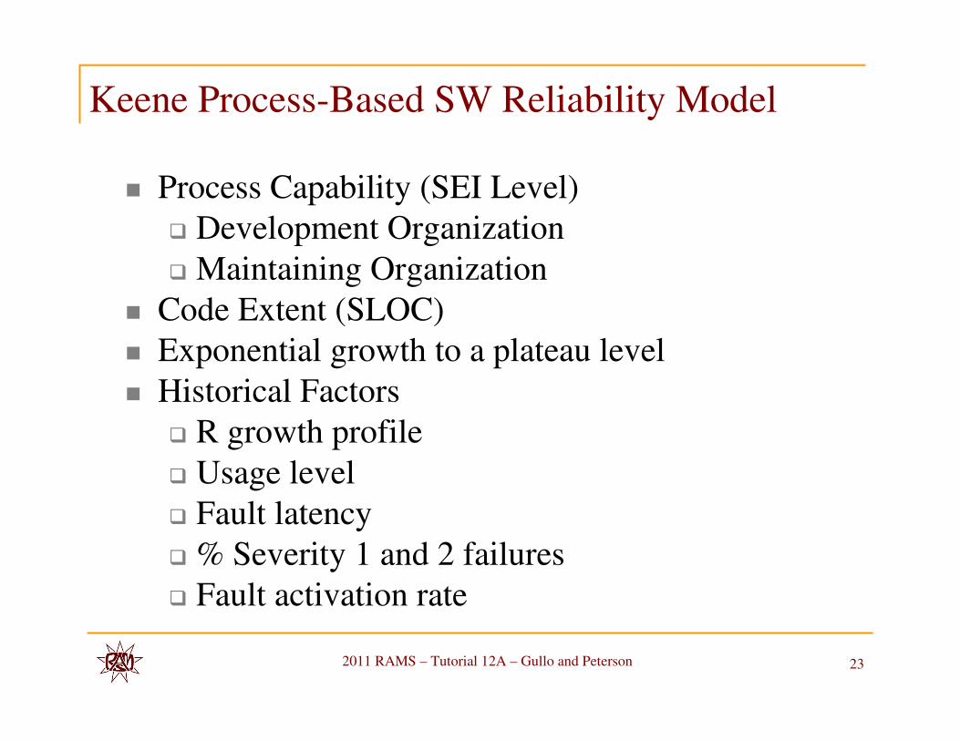
Keene Process-Based SW Reliability Model
� Process Capability (SEI Level)
� Development Organization
� Maintaining Organization
� Code Extent (SLOC)
� Exponential growth to a plateau level
� Historical Factors
� R growth profile
� Usage level
� Fault latency
� % Severity 1 and 2 failures
� Fault activation rate

2011 RAMS – Tutorial 12A – Gullo and Peterson 24
The Importance of Process
Conclusion: Design, Software, Requirements
Management, Quality of Communications between
Groups, and the Development Process are the major
drivers of software and system reliability.

2011 RAMS – Tutorial 12A – Gullo and Peterson 25
Capability Maturity Model
SEI LevelsLevel Description of Organization
Level 1:
Initial
Organizations lack effective project management; do not
maintain a solid, stable environment …
Level 2:
Repeatable
Organizations maintain policies and procedures for managing
and developing ... Project planning based upon experience …
Level 3:
Defined
Organizations have developed and documented a standard
process for managing and developing software systems....
Level 4:
Managed
Organizations set quantitative goals … use measurement
instruments to collect process and product metrics.
Level 5:
Optimizing
Organizations focus on continuous process improvement…

2011 RAMS – Tutorial 12A – Gullo and Peterson 26
Fault Discovery and Reliability Growth
� Reliability growth reasonably follows the exponential growth pattern over deployment
� The best documentation at time of analysis was Chillarege’s paper reporting 4 year maturation cycle on AIX when delivered and 2 years for updates – big operating system
� Latest data from Dr Keene (2005 data) for software growth to maturity stage suggests a 2 year period – depends on the operating system
� Calculate Reliability Growth: F = N*e-λλλλ t
F = Faults remaining at Maturity
N = Initial Faults
The number of faults is assumed to follow an exponential function

2011 RAMS – Tutorial 12A – Gullo and Peterson 27
Keene Development Process Software Prediction
Model Results Correlation Curt Smith ISSRE 99
0
50
100
150
200
250
300
350
400
450
500
550
600
650
700F
eb
-96
Ma
r-9
6
Ap
r-9
6
Ma
y-9
6
Ju
n-9
6
Ju
l-9
6
Au
g-9
6
Se
p-9
6
Oc
t-9
6
No
v-9
6
De
c-9
6
Ja
n-9
7
Fe
b-9
7
Ma
r-9
7
Ap
r-9
7
Ma
y-9
7
Ju
n-9
7
Ju
l-9
7
Au
g-9
7
Se
p-9
7
Oc
t-9
7
No
v-9
7
De
c-9
7
Ja
n-9
8
Fe
b-9
8
Ma
r-9
8
Ap
r-9
8
So
ftw
are
Err
ors
Re
ma
inin
g / 1
00
KS
LO
C
SWEEP actuals
SWEEP prediction
CASRE actuals
Generalized Poisson estimate
DPM prediction
91%
99%
35%
DPM = Development Process Model
Figure reproduced by permission of the author and the IEEE © 10th International Symposium on Software Reliability Engineering
Actual data supports the Rayleigh Model
2011 RAMS – Tutorial 12A – Gullo and Peterson 28
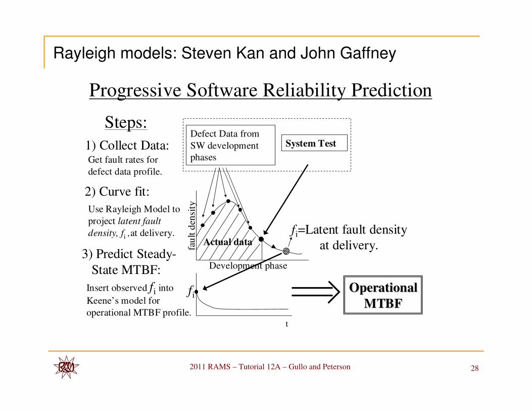
Progressive Software Reliability Prediction
1) Collect Data:Defect Data from
SW development
phases
System Test
2) Curve fit:
Steps:
3) Predict Steady-
State MTBF:
Get fault rates for
defect data profile.
fau
lt d
ensi
tyUse Rayleigh Model to
project latent fault
density, fi ,at delivery. fi=Latent fault densityat delivery.
Insert observed fi into
Keene’s model for
operational MTBF profile.t
fiOperationalOperational
MTBFMTBF
Development phase
Actual data
Rayleigh models: Steven Kan and John Gaffney

2011 RAMS – Tutorial 12A – Gullo and Peterson 29
Capability Maturity Model
Fault Density at Delivery Studies
� Fault density is in defects per thousand lines of code (KSLOC).
� Data represents average expected results gathered from several SEI rated companies.
CMM
LEVEL
FAULTS/KSLOC
(Keene Data)
FAULTS/KSLOC
(Caper Jones)
FAULTS/KSLOC
(Herb Krasner)Defect Plateau Level
V 0.5 0.5 0.5 1.5%
IV 1.0 1.4 2.5 3.0%
III 2.0 2.69 3.5 5.0%
II 3.0 4.36 6.0 7.0%
I 5.0 7.44 30 10.0%

2011 RAMS – Tutorial 12A – Gullo and Peterson 30
Capability Maturity Model
Calculating Reliability Growth

2011 RAMS – Tutorial 12A – Gullo and Peterson 31
Keene Process-Based (a priori) SW Reliability
Model (CMM Model) Inputs
• This model provides MTBF and Ao predictions that are used to allocate
requirements and confirm that the requirements were
obtainable.
• These predictions are
somewhat approximate, and so further refinement is needed in the later
stages of the process.
� Process Capability (SEI Level)
� Development Organization
� Maintaining Organization
� Code Extent (SLOC)
� Exponential growth to a plateau level
� Historical Factors
� R growth profile
� Usage level
� Fault latency
� % Severity 1 and 2 failures
� Fault activation rate

2011 RAMS – Tutorial 12A – Gullo and Peterson 32
Keene Process-Based (a priori) SW Reliability
Model (CMM Model) Inputs
Data Required Inputs Range Input Instructions: KSLOCs 441.7 >0 Number KSLOCsSEI Level - Develp 3 1-5 SEI Level factor (1-5). SEI Level - Maint. 3 1-5 SEI Level factor (1-5).
Months to maturity 20 <=48Number of months to maturity or failure rate plateau.
Use hrs/week 168 <=168 Number of operational hours/week
% Fault Activation 100 <=100Ave. %population exhibiting fault activation.
Fault Latency 2 >=1Ave. # of fault reoccurrences/failing-site until corrected.
% Sev 1&2 Fail 10 <=100Ave. % severity 1 and 2 or % countable failures.
MTTR 10 >0 Ave. Time to restore system (minutes)
Process Input Parameters

2011 RAMS – Tutorial 12A – Gullo and Peterson 33
Capability Maturity Model
Available Tools
� Excel Spreadsheet
� MathCad Worksheet
� Database Application

2011 RAMS – Tutorial 12A – Gullo and Peterson 34
Capability Maturity Model
Example
� Assumptions:
� SEI Level 4 process was followed during development, which gives a fault density of 1.
� SEI Level 4 process was followed during maintenance, which gives a steady state of 3.0% of the initial fault density.
Module KSLOC
Total Defects
At Delivery
Defects At
Steady State
A 208 208 3.12

2011 RAMS – Tutorial 12A – Gullo and Peterson 35
Capability Maturity Model
Data Table Example
� Critical defects are assumed to be 7.93% of the total populationbased on historical information.
� Critical defect is defined as priority 1 or 2 per Mil Std. 2167.
Month MTBF
(Hrs)
Faults
Remaining
Faults
Discovered
Critical
MTBF
Fault
Density
Failure
Rate
Availability
0 48.04 208.00 0 605.82 1.0000 0.00165 0.9995875
1 51.68 193.42 14.58 651.74 0.9299 0.00153 0.9996165
2 55.60 179.87 13.55 701.13 0.8648 0.00142 0.9996435
3 59.81 167.26 12.60 754.27 0.8042 0.00132 0.9996686
4 64.35 155.54 11.72 811.43 0.7478 0.00123 0.9996919
5 69.22 144.64 10.90 872.93 0.6954 0.00114 0.9997136
6 74.47 134.51 10.14 939.09 0.6467 0.00106 0.9997338

2011 RAMS – Tutorial 12A – Gullo and Peterson 36
SWEEP (Software Error Estimation Program)
Topics of Discussion
� SWEEP Capabilities
� SWEEP Assumptions
� SWEEP Model Theory
� SWEEP Features
� Where to Find SWEEP
� Questions

2011 RAMS – Tutorial 12A – Gullo and Peterson 37
SWEEP Capabilities
� The SWEEP tool enables you to:
� Predict and track the rate at which defects will be found
� Predict the latent defect content of software products.
� Analyze estimated errors injected in each phase of the software
development cycle
� Determine the detection effectiveness and leakage of errors to
subsequent phases.
� Measure percentage of critical failures that feedback into the
Keene model
� SWEEP Data Collection
� Data is typically collected using Software Trouble Reports (STR)
� Data can be organized by development phase or time increments.

2011 RAMS – Tutorial 12A – Gullo and Peterson 38
SWEEP Model Assumptions
� All detected defects are recorded when they are detected.
� Defects are fixed when they are discovered.
� Defects are tracked consistently.
� If you track a certain type of defect in the design phase, then you must track the same type of defect throughout the life cycle.
� Defects in software documentation are not tracked with functional software defects. Documentation defects incorrectly inflate the latent defect content of the software product.
� The data input into SWEEP is validated and updated on a regular basis.

2011 RAMS – Tutorial 12A – Gullo and Peterson 39
SWEEP Model Theory
� The SWEEP Tool uses the Rayleigh Model
� The Rayleigh Distribution is a special case of the Weibull Distribution
� Model Assumptions
� The defect rate observed during the development process is positively correlated with the defect rate in the field (The more area under the curve, the higher the field defect rate).
� Given the same error injection rate, if more defects are discovered and removed earlier, fewer will remain in later stages.
� Reference Reading Metrics and Models in Software Quality Engineering, Addison Wesley Publishing

2011 RAMS – Tutorial 12A – Gullo and Peterson 40
SWEEP Model Theory
Time
SEI Level I
SEI Level II
SEI Level III
SEI Level IV
SEI Level VDefect Rate
2011 RAMS – Tutorial 12A – Gullo and Peterson 41
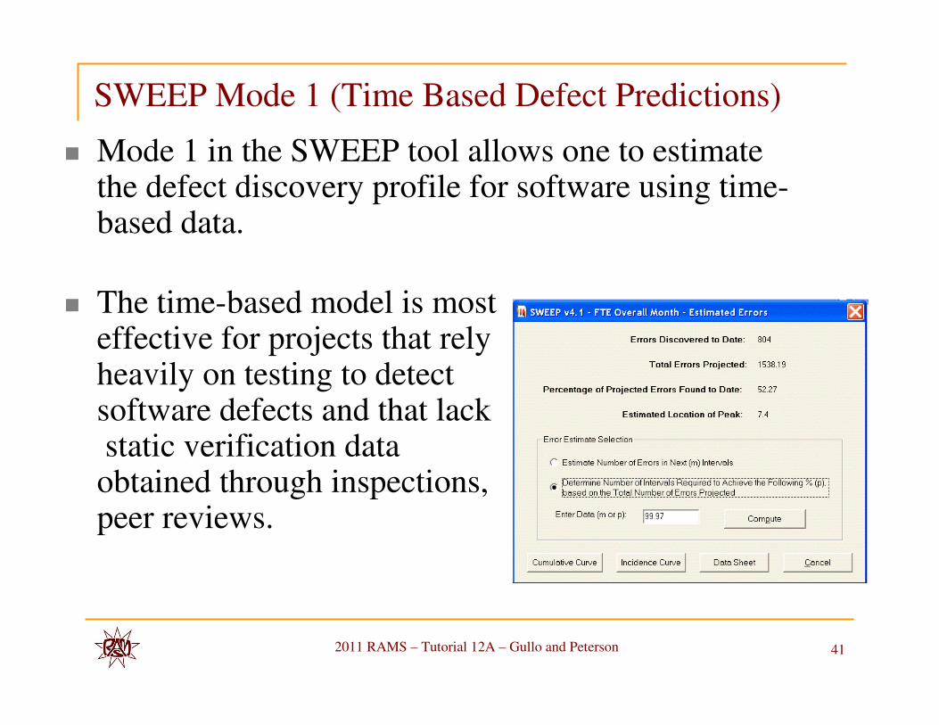
SWEEP Mode 1 (Time Based Defect Predictions)
� Mode 1 in the SWEEP tool allows one to estimate the defect discovery profile for software using time-based data.
� The time-based model is most effective for projects that rely heavily on testing to detect software defects and that lackstatic verification data obtained through inspections, peer reviews.

2011 RAMS – Tutorial 12A – Gullo and Peterson 42
SWEEP Mode 1 (Time Based Defect Predictions)
� Mode 1 answers questions such as:
� What are the estimated remaining defects after N more test intervals?
� How many more test intervals are needed to remove X percentage of projected defects?
� When will system testing finish?
� When can the software product be shipped?
2011 RAMS – Tutorial 12A – Gullo and Peterson 43
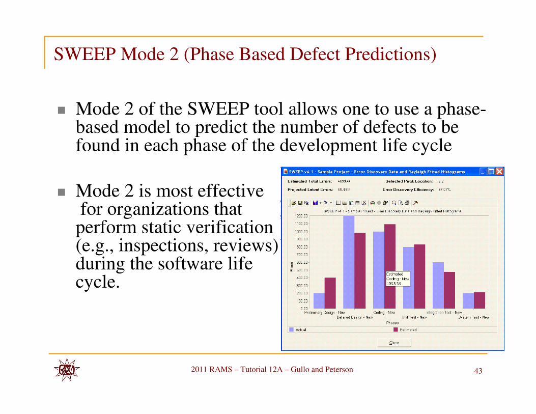
SWEEP Mode 2 (Phase Based Defect Predictions)
� Mode 2 of the SWEEP tool allows one to use a phase-based model to predict the number of defects to be found in each phase of the development life cycle
� Mode 2 is most effectivefor organizations that perform static verification (e.g., inspections, reviews)during the software life cycle.

2011 RAMS – Tutorial 12A – Gullo and Peterson 44
SWEEP Mode 2 (Phase Based Defect Predictions)
� Mode 2 has the following advantages over Mode 1:
� One can plan and schedule testing activities more accurately for later phases of development due to earlier prediction of defects.
� One can use defect data to predict the discovery of defects in later phases of the development life cycle.
� One can predict defects before your software is in an executable state.
� The organization can compare the defect discovery histories for various software products.
2011 RAMS – Tutorial 12A – Gullo and Peterson 45
Where To Find SWEEP?
� SWEEP (Software Error Estimation Program) is available through the Software Productivity Consortium.
� Free tool to members and is available on their web site.
http://www.software.org
� If your company is a member of the software productivity consortium, complete web site access is available by requesting an account and password.

2011 RAMS – Tutorial 12A – Gullo and Peterson 46
SWEEP Tool Demonstration
1. Time based data example.
2. Phase based data example
3. Questions

2011 RAMS – Tutorial 12A – Gullo and Peterson 47
CASRE (Computer Aided Software Reliability Estimation)
Topics for Discussion
� CASRE Introduction
� CASRE Applicability
� Software Reliability Process
� Software Reliability Models
� CASRE Data Input
� CASRE Tool Demonstration
� Questions

2011 RAMS – Tutorial 12A – Gullo and Peterson 48
CASRE Introduction
� CASRE (Computer Aided Software Reliability
Estimation)
� Software reliability measurement tool
� Runs in the Microsoft Windows environment
� Develop by Allen Nikora at JPL.
� The modeling and analysis capabilities of CASRE are
provided SMERFS (Statistical Modeling and
Estimation of Reliability Functions for Software).
� In CASRE, the original SMERFS user interface has
been discarded, and the SMERFS modeling libraries
are linked into the new CASRE user interface

2011 RAMS – Tutorial 12A – Gullo and Peterson 49
CASRE Applicability
� CASRE is typically applied starting after unit test and continuing through system test, acceptance test, and operations.
� You should only apply CASRE to modules for which you expect to see at least 40 or 50 failures. If you expect to see fewer failures, you may reduce the accuracy of your estimates.
� Experience shows that at the start of software test, modules having more than about 2000 source lines of executable code will tend to have enough faults to produce at least 40 to 50 failures.

2011 RAMS – Tutorial 12A – Gullo and Peterson 50
Software Reliability Models
� Software reliability models are statistical models
used to make predictions about a software system's
failure rate, given the failure history of the system.
� The models make assumptions about the fault
discovery and removal process. These assumptions
determine the form of the model and the meaning
of the model's parameters.
� There are two types of models:
1. Predict times between failures
2. Predict the number of failures that will be found
in future test intervals.
2011 RAMS – Tutorial 12A – Gullo and Peterson 51
CASRE Data Input
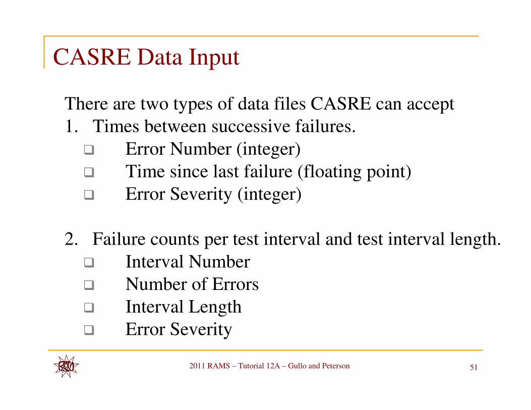
There are two types of data files CASRE can accept
1. Times between successive failures.
� Error Number (integer)
� Time since last failure (floating point)
� Error Severity (integer)
2. Failure counts per test interval and test interval length.
� Interval Number
� Number of Errors
� Interval Length
� Error Severity

2011 RAMS – Tutorial 12A – Gullo and Peterson 52
Accuracy
Information to enhance the accuracy of model predictions:
� Date and time at which each failure was found, and the test interval during which the software was run that produced that failure.
� Date and time at which the testing method changed. The reason for this is that the perceived reliability of the system depends on how it is executed.
� Date and time at which the test environment changed. The reason for collecting this information is to more accurately characterize the length of a test interval.
� Date and time at which the software being tested changes significantly.
� Severity of each failure.

2011 RAMS – Tutorial 12A – Gullo and Peterson 53
Sample CASRE Data Models and OutputModule A Actuals Vs CASRE Model Fit
0
2000
4000
6000
8000
10000
12000
14000
16000
18000
20000
1 2 3 4 5 6 7 8 9 10 11 12 13 14 15 16 17 18 19 20 21 22 23
Event
Tim
e B
etw
een
Even
ts (
Hrs
) Actual Time Betw een Failure Events
CASRE Model Curve Fit
Failure Counts ModelsGeneralized PoissonSchneidewindShick-WolvertonYamada S-shaped
Times Between Failures ModelsGeometricJelinski-MorandaLittlewood-Verrall LinearLittlewood-Verrall Quadratic* Musa BasicMusa-Okumoto *
All Data is Notional

2011 RAMS – Tutorial 12A – Gullo and Peterson 54
CASRE Model Selection Criteria
Time between failures
Prequential likelihood,
Relative accuracy,
Model bias,
Model bias trend,
Bias scatter plot,
Model noise,
Kolmogorov - Smirnov test statistic
Failure counts
Prequential likelihood,
Relative accuracy,
Chi-Square test statistic
Maximum Likelihood Estimation

2011 RAMS – Tutorial 12A – Gullo and Peterson 55
CASRE Model Selection Criteria
Least Squares Estimation
Time between failures
Kolmogorov - Smirnov
test statistic
Failure counts
Chi-Square test
statistic

2011 RAMS – Tutorial 12A – Gullo and Peterson 56
CASRE Model Assumptions - Time To Failure Models
Geometric model
1.The software is operated in a similar manner as the
anticipated operational usage.
2.The detections of faults are independent of one
another.
3.There is no upper bound on the total number of failures
(i.e., the program will never be error-free).
4.All faults do not have the same chance of detection.
5.The detections of faults are independent of one
another.
6.The failure detection rate forms a geometric
progression and is constant between failure
occurrences.

2011 RAMS – Tutorial 12A – Gullo and Peterson 57
CASRE Model Assumptions - Time To Failure Models
Jelinski-Moranda model
1.The software is operated in a similar manner to the
anticipated operational usage.
2.All failures are equally likely and independent.
3.Rate of failure detection is proportional to the current
fault content.
4. All failures are of the same order of severity
5. Failure rate remains constant over the interval between
failure occurrences.
6.Faults are corrected instantaneously without introduction
of new faults into the program.
7.The total number of failures expected has an upper bound.

2011 RAMS – Tutorial 12A – Gullo and Peterson 58
CASRE Model Assumptions Time To Failure Models
Musa Basic Model1.The software is operated in a similar manner to the
anticipated operational usage.
2. Failure detections are independent of one another.3. All software failures are observed (i.e., the total
number of failures has an upper bound).4.The execution times between failures are piecewise
exponentially distributed.5.The hazard rate is proportional to the number of faults
remaining in the program.
6.Fault correction rate is proportional to the failure rate.7.Perfect debugging is assumed.

2011 RAMS – Tutorial 12A – Gullo and Peterson 59
CASRE Model Assumptions Time To Failure Models
Musa-Okumoto Model
1.The software is operated in a similar manner as
the anticipated operational usage.
2.The detections of failures are independent of one
another.
3.The expected number of failures is a logarithmic
function of time.
4.The failure intensity decreases exponentially with
the expected number of failures experienced.
5.There is no upper bound on the number of total
failures (i.e., the program will never be error-free).

2011 RAMS – Tutorial 12A – Gullo and Peterson 60
CASRE Model AssumptionsFailure Count Models
Generalized Poisson Model (includes Schick-Wolverton Model):
1. The software is operated in a similar manner as the
anticipated operational usage.2. Failures are equally likely and are independent
3. Expected number of failures occurring in any time interval is proportional to the fault content at the time
of testing, and a function of the time spent in testing.4. Each failure is of the same order of "severity" as any
other failure.
5. Faults are corrected at the ends of the testing intervals, without introducing new faults.

2011 RAMS – Tutorial 12A – Gullo and Peterson 61
CASRE Model AssumptionsFailure Count Models
Schneidewind Model (all three variants):1. The software is operated in a similar manner as the
anticipated operational usage.2. Failures are equally likely and independent3. Fault correction rate is proportional to the number of faults.4. Mean number of failures decreases from one testing interval
to the next. Total number of failures has an upper bound.5. All testing periods are of the same length.6. Rate of fault detection is proportional to the number of faults
in the program at the time of test. Failure detection is a non-homogeneous Poisson process with exponentially decreasing failure rate.
7. Perfect debugging is assumed.

2011 RAMS – Tutorial 12A – Gullo and Peterson 62
Yamada S-shaped model:1.The software is operated in a similar manner as the
anticipated operational usage.
2. A software system is subject to failures at random caused by faults present in the system.
3.Initial fault content of the system is a random variable.4.The time between failures (k - 1) and k depends on the
time to failure (k - 1).5.Each time a failure occurs, the fault which caused it is
immediately removed; no new faults are introduced.
6.Total number of failures expected has an upper bound.
CASRE Model AssumptionsFailure Count Models

2011 RAMS – Tutorial 12A – Gullo and Peterson 63
CASRE Demonstration
1. Times between successive failures example.
2. Failure counts per test interval example
3. Questions

2011 RAMS – Tutorial 12A – Gullo and Peterson 64
How Do I Acquire CASRE?
You may obtain a copy of CASRE and its documentation
at the following web address:
http://www.openchannelfoundation.org/projects/CASRE
_3.0/

2011 RAMS – Tutorial 12A – Gullo and Peterson 65
� The product represents a typical commercial off-the-shelf electro-mechanical device manufactured in high volume for a global marketplace
� A test that detects failures which would ultimately have an impact on product reliability and performance in the field in the hands of a customer has the potential of providing value to the business
� Actual value is obtained only when the failures are isolated and corrected.
� Value obtained by warranty cost avoidance and customer satisfaction with continued business.
Business Case Study

2011 RAMS – Tutorial 12A – Gullo and Peterson 66
AST Results
� Seven (7) test starts “stages” were performed
� Stages 1-4 did not meet 300k goal
� During the first 3 starts, a software pattern failure
developed
� Demonstrated MCBF was 30.9k cycles
� Failure rate = 32.3 fails/million cycles
� Cycles/unit and cycles-to-failure data

2011 RAMS – Tutorial 12A – Gullo and Peterson 67
Stage 1-4 Failure Data (Cycles)
Unit Initial start
15,037
cycles
2nd start
45,037
cycles
3rd start
59,101 cycles
Total
Cycles
~300,000
cycles
Total Failures
1 15,037 23,437
“S11”
37,501 285,736 Software failure
2 8,750 “S3” 9,950 “S8” 10,550 “G3” 10,550 Gear + 2 s/w fails
3 14,750 “S7” 44,700 58,550 “S20” 306,631 2 s/w failures
…
15 15,037 36,637
“S14”
50,701 298,936 Software failure
16 15,037 45,037 52,237 “S18” 300,318 Software failure
Total
Failures8 9 6 5 28

2011 RAMS – Tutorial 12A – Gullo and Peterson 68
Probabilistic Software Failure Example
� 2ms window for failure occurrence
65ms function occurrence
� Probability of Failure
(Pf) = 1/ 32,768 = 3.05 x 10E-5 = 0.00305%
� Probability of Success
(Ps) = 1 – Pf = 0.999969; or 99.99695%
These calculated results closely match the empirical results from the Weibull model

2011 RAMS – Tutorial 12A – Gullo and Peterson 69
//**************************************************TIMER INTERRUPT ROUTINE
//**************************************************Interrupt routine // Called every 65mS{
Increment CounterIf (Counter > max value){
TimeOut Bit = TRUE;}
}//**************************************************
Pseudocode

2011 RAMS – Tutorial 12A – Gullo and Peterson 70
//***********************************************************MAIN PROGRAM
//***********************************************************Start TimeOut Routine{
Clear TimeOut Bit Clear Counter
}Start Mechanical Arm travelWhile ( Arm NOT at final destination AND TimeOut bit is FALSE){if (TimeOut Bit is TRUE){
Do Error Routine}
}//***********************************************************
Pseudocode

2011 RAMS – Tutorial 12A – Gullo and Peterson 71
Warranty Cost Avoidance Model
� Warranty cost model = ΣΣΣΣ[(FR x V x AFU) x P x C]
� Model Assumptions:
� Average Field Usage (AFU) is 100 cycles/day, equating to 36,500 cycles/unit
� Production fix put into place after 4 months of field reports
� Volume (V) = 27,000 annual sales => sold 9000 in first 4 months of product launch
� 4,500 in inventory
� Rework inventory required once problem was found
� Software errors in first year of usage:
� 10,610 software errors-fails/yr (FR x V x AFU)
2011 RAMS – Tutorial 12A – Gullo and Peterson 72
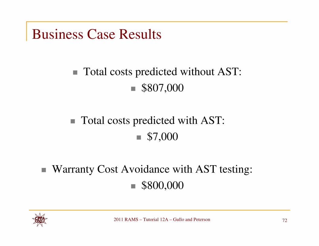
Business Case Results
� Total costs predicted without AST:
� $807,000
� Total costs predicted with AST:
� $7,000
� Warranty Cost Avoidance with AST testing:
� $800,000

2011 RAMS – Tutorial 12A – Gullo and Peterson 73
SW Reliability Reference Books
� Metrics and Models in Software Quality Engineering, Stephen Kan, Addison Wesley Publishing
� Handbook of Software Reliability Engineering, Michael Lyu, McGraw Hill Publishing
� Software Reliability: Measurement, Prediction, Application, John D. Musa, Anthony Iannino, and Kazuhira Okumoto, McGraw-Hill Book Company
� IEEE 1633: Recommended Practice on Software Reliability (SR)
� IEC 62628: Guidance on Software Aspects of Dependability

2011 RAMS – Tutorial 12A – Gullo and Peterson 74
Considerations Incorporating Software
Reliability Into System Ao Modeling

2011 RAMS – Tutorial 12A – Gullo and Peterson 75
Operational Availability (Ao)
�Ao is the ratio of Up Time to Total Time, where total
time includes Up Time and Down Time.
�Down Time includes all time when the program is
not functional.
�Total Time is the sum of Up Time and Down Time.
IOSMTBF
MTBF
Time RunTotal
Time Recovery - Time RunTotal
Time DownTime Up
Time UpAo
+=
=+
=

2011 RAMS – Tutorial 12A – Gullo and Peterson 76
Software Ao Modeling
Ao (Software) Ao (Hardware)
Typical Reliability Block Diagram (RBD)
Single Serial System

2011 RAMS – Tutorial 12A – Gullo and Peterson 77
Software Ao Modeling
Ao (Hardware)
Typical RBD
Parallel System With Independence Assumption
1:2
Ao (Software)
Ao (Hardware)Ao (Software)
2011 RAMS – Tutorial 12A – Gullo and Peterson 78
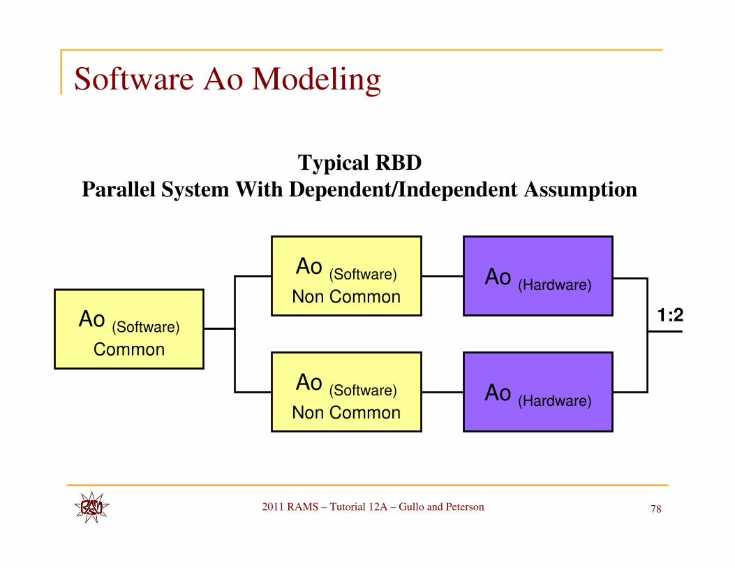
Software Ao Modeling
Typical RBD
Parallel System With Dependent/Independent Assumption
Ao (Hardware)
1:2
Ao (Software)
Non Common
Ao (Hardware)Ao (Software)
Non Common
Ao (Software)
Common

2011 RAMS – Tutorial 12A – Gullo and Peterson 79
Sample Ao - System to Software Configuration Item
� Accumulated average Ao Measurements
� Measurements assess results at different levels in the system hierarchy – the three levels are:
� System
� Component = Multiple SCIs
� Software Configuration Item (SCI)
System
Measured
Ao
Spec
Ao Component
Measured
Ao Spec Ao SCI
Measured
Ao
Specified
Ao
A1 A1-1 0.9999999 0.99989
A1-2 0.9999998 0.99989
A2 A2-1 0.9999998 0.99989
A2-2 0.9999994 0.99989
A3 A3-1 0.9999989 0.99979
A3-2 0.9999993 0.99986
0.99978
0.99978
0.99965
A 0.9999971 0.999 0.9999997
0.9999993
0.9999981

2011 RAMS – Tutorial 12A – Gullo and Peterson 80
Sample Results – Ao by Month
Demonstrates Traditional Growth Curve
0.95
0.955
0.96
0.965
0.97
0.975
0.98
0.985
0.99
0.995
1
Aug-0
8Sep
-08
Oct
-08
Nov
-08
Dec
-08
Jan-
09Feb
-09
Mar
-09
Apr-0
9M
ay-0
9Ju
n-09
Jul-0
9Aug
-09
Sep-0
9O
ct-0
9N
ov-0
9D
ec-0
9Ja
n-10
Feb-1
0M
ar-1
0Apr
-10
Peaks demonstrate the
Test Analyze and Fix
(TAAF)
Methodology

2011 RAMS – Tutorial 12A – Gullo and Peterson 81
Limitations
� Not applicable to one-shot systems
� Software embedded in a one-shot system is different from software in
a large or complex system
� Reliability is the critical performance parameter, but the system
model is different from a system with a large mission times
� The entire software reliability growth process decreases value-added
benefits as the software programs get smaller and less complex
� < 2KSLOCs
� < 10 I/Os
� < 1 hr Mission Time
� State Machine vs Asynchronous Complex Systems
2011 RAMS – Tutorial 12A – Gullo and Peterson 82
Conclusions
� Goals for the Training
� Software Reliability Process
� Capability Maturity Model (Keene Model)
� Rayleigh Model Analysis
� Software Error Estimation Program (SWEEP)
� Computer Aided Software Reliability Estimation
� Business Case Study
� Incorporating Software Reliability Into System Ao Modeling
� Limitations