Looking back, What’s ahead

Looking back, What’s ahead

Yves Robert Per Stenstrom Viktor K. Prasanna

December 15, 2011

1

Chapter 1

Looking Back at Dense Linear AlgebraSoftware

Piotr Luszczek

Jakub Kurzak

Jack Dongarra

Abstract

Over the years, computational physics and chemistry served as an ongoing source of problems that

demanded the ever increasing performance from hardware as well as the software that ran on top of

it. Most of these problems could be translated into solutions for systems of linear equations: the very

topic of numerical linear algebra. Seemingly then, a set of efficient linear solvers could be solving

important scientific problems for years to come. We argue that dramatic changes in hardware designs

precipitated by the shifting nature of the marketplace of computer hardware had a continuous effect

on the software for numerical linear algebra. The extraction of high percentages of peak performance

continues to require adaptation of software. If the past history of this adaptive nature of linear algebra

software is any guide then the future theme will feature changes as well – changes aimed at harnessing

the incredible advances of the evolving hardware infrastructure.

1.1 Introduction

Over the decades, dense linear algebra has been an indispensible component of science and engineer-ing. While the mathematical foundations and application methodology has changed little, the hardwarehas undergone a tumultous transition. The latter precipitated a number of paradigm shifts in the waythe linear algebra software is implemented. Indeed, the ever evolving hardware would quickly render oldcode inadequate in terms of performance. The external interfaces to the numerical software routineshave undergone only minor adjustment which is in line with the unchanged mathematical forumlationof the problem of solving a system of linear equations. The internal implementation of these interfaceswas changing to accomodate drastic redesign of the underlying hardware technology. The internalshave been modularized to ease the implementation process. These modules over time have become thebuilding blocks of new generations of the numerical linear algebra libraries and made the effort moremanagable in the long run. Over time, the number and functionality of these building blocks haveincreased but the delegation of responsibilities between various modules inside the software stack hasbeen retained. The most recent increase in hardware parallelism further altered the established compo-sition process of the modules by necessitating the use of explicit scheduling mechanism which neededto be handled manually in the compositing code or externally with a software scheduler. The rapidtransformation of computer hardware has not been ongoing and is expected to be continuing into thefuture. With it, the software will evolve further and our hope is that the design decision made in thepast will allow for a smooth transition by reusing the tested and optimized libraries we have becomeaccustomed to.

3

4 Looking Back at Dense Linear Algebra Software

1.2 Motivation: Plasma Physics and Electronic Structure Calculation

Computational experiments of self-sustaining fusion reactions could give us an informed perspectiveon how to build a device capable of producing and controlling the high performance [1]. Modeling theheating response of plasma due to radio frequency (RF) waves in the fast wave time scale leads to solvingthe generalized Helmholtz equation. The time harmonic terms of effective approximations of the electricfield, magnetic field, and distribution function as a time-averaged equilibrium satisfy the equation.The Scientific Discovery through Advanced Computing project (SciDAC) Numerical Computation ofWave Plasma-Interactions in Multi-dimensional Systems developed and implemented a simulation codethat gives insight into how electromagnetic waves can be used for driving current flow, heating andcontrolling instabilities in the plasma. The code is called AORSA [2, 3, 4, 5, 6] and stands for All ORdersSpectral Algorithm. The resulting computation requires a solution of a system of linear equationsexceeding half a million unknowns [7].

In quantum chemistry, most of the scientific simulation codes result in a numerical linear algebraproblem that may readily be solved with the ScaLAPACK library [8, 9]. For example, early versions ofParaGauss [10, 11, 12, 13] relied on diagonalization of the Kohn-Sham matrix and the parallelizationmethod of choice relied on the irreducible representations of the point group. The submatrices diago-nalize in parallel and the number of them depended on the symmetry group. When using one of ScaLA-PACK’s parallel eigensolvers it is possible to achieve speedup even for a Kohn-Sham matrix with onlyone block. A different use of the BLAS library occurs in UTChem [14] – an application code that collectsa number of methods that allow for accurate and efficient calculations for computational chemistry ofelectronic structure problems. Both the ground and excited states of molecular systems are covered.In supporting a number of single-reference many-electron theories such as configuration-interactiontheory, coupled-cluster theory, and Møller-Plesset perturbation theory, UTChem derives working equa-tions using a symbolic manipulation program called Tensor Contraction Engine (TCE) [15]. It automatesthe process of deriving final formulas and generation of the execution program. The contraction of cre-ation and annihilation operators according to Wick’s theorem, consolidation of identical terms, andreduction of the expressions into the form of tensor contractions controlled by permutation operatorsare all done automatically by TCE. If tensor contractions are treated as a collection of multi-dimensionalsummations of the product of a few input arrays then the commutative, associative, and distributiveproperties of the summation allow for a number of execution orders, each of which having different ex-ecution rates when mapped to a particular hardware architecture. Also, some of the execution orderswould result in calls to BLAS, which provides a substantial increase in floating-point execution rate.The current TCE implementation generates many-electron theories that are limited to non-relativisticHartree-Fock formulation with reference wave functions but it is possible to extend it to relativistic 2-and 4-component reference wave functions.

1.3 Problem Statement in Matrix Terms

Most dense linear systems solvers rely on a decompositional approach [16]. The general idea is thefollowing: given a problem involving a matrix A, one factors or decomposes A into a product of simplermatrices from which the problem can easily be solved. This divides the computational problem into twoparts: first determine an appropriate decomposition, and then use it in solving the problem at hand.Consider the problem of solving the linear system:

Ax = b (1.1)

where A is a nonsingular matrix of order n. The decompositional approach begins with the observationthat it is possible to factor A in the form:

A = LU (1.2)

where L is a lower triangular matrix (a matrix that has only zeros above the diagonal) with ones on thediagonal, and U is upper triangular (with only zeros below the diagonal). During the decompositionprocess, diagonal elements of A (called pivots) are used to divide the elements below the diagonal. Ifmatrix A has a zero pivot, the process will break with division-by-zero error. Also, small values of thepivots excessively amplify the numerical errors of the process. So for numerical stability, the methodneeds to interchange rows of the matrix or make sure pivots are as large (in absolute value) as possible.

1.4. Introducing LU: a Simple Implementation 5

This observation leads to a row permutation matrix P and modifies the factored form to:

PA = LU (1.3)

The solution can then be written in the form:

x = A−1Pb (1.4)

which then suggests the following algorithm for solving the system of equations:

• Factor A according to Eq. (1.3)

• Solve the system Ly = Pb

• Solve the system Ux = y

This approach to matrix computations through decomposition has proven very useful for several rea-sons. First, the approach separates the computation into two stages: the computation of a decompo-sition, followed by the use of the decomposition to solve the problem at hand. This can be important,for example, if different right hand sides are present and need to be solved at different points in theprocess. The matrix needs to be factored only once and reused for the different right hand sides. Thisis particularly important because the factorization of A, step 1, requires O(n3) operations, whereas thesolutions, steps 2 and 3, require only O(n2) operations. Another aspect of the algorithm’s strength is instorage: the L and U factors do not require extra storage, but can take over the space occupied initiallyby A. For the discussion of coding this algorithm, we present only the computationally intensive partof the process, which is step 1, the factorization of the matrix.

Decompositional technique can be applied to many different matrix types:

A1 = LLT A2 = LDLT PA3 = LU A4 = QR (1.5)

such as symmetric positive definite (A1), symmetric indefinite (A2), square non-singular (A3), and generalrectangular matrices (A4). Each matrix type will require a different algorithm: Cholesky factorization,Cholesky factorization with pivoting, LU factorization, and QR factorization, respectively.

1.4 Introducing LU: a Simple Implementation

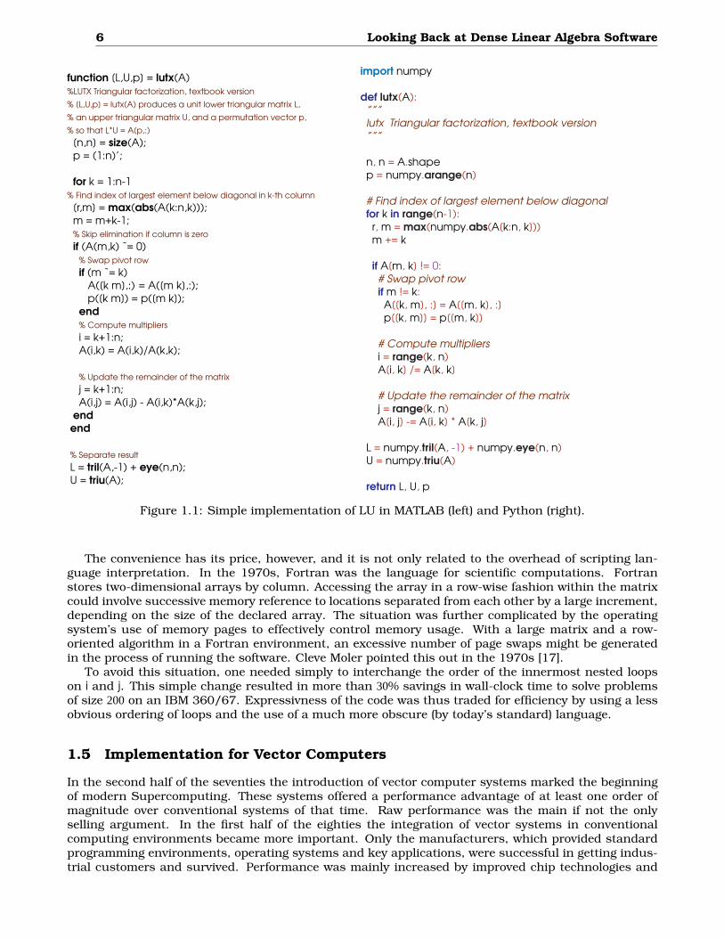
For the first version, we present a straightforward implementation of LU factorization. It consists ofn—1 steps, where each step introduces more zeros below the diagonal, as shown in Figure 1.1.

Tools often used to teach Gaussian elimination include MATLAB and Python. They are scriptinglanguages that make developing matrix algorithms very simple. The notation might seem very unusualto people familiar with other scripting languages because it is oriented to process multidimensionalarrays. The unique features of the language that we use in the example code are:

• Transposition operator for vectors and matrices: ’ (single quote)

• Matrix indexing specified as:

– Simple integer values: A(m, k)

– Ranges: A(k:n, k)

– Other matrices: A([k m], : )

• Built-in matrix functions such as size or shape (returns matrix dimensions), tril (returns the lowertriangular portion of the matrix), triu (returns the upper triangular portion of the matrix), and eye(returns an identity matrix, which contains only zero entries, except for the diagonal, which is allones).

The algorithm presented in Figure 1.1 is row-oriented, in the sense that we are taking a scalarmultiple of the “pivot” row and adding it to the rows below to introduce zeros below the diagonal. Thebeauty of the algorithm lies in its similarity to the mathematical notation. Hence, this is the preferredway of teaching the algorithm for the first time so that students can quickly turn formulas into runningcode.


function [L,U,p] = lutx(A)%LUTX Triangular factorization, textbook version

% [L,U,p] = lutx(A) produces a unit lower triangular matrix L,

% an upper triangular matrix U, and a permutation vector p,

% so that L*U = A(p,:)

[n,n] = size(A);p = (1:n)’;

for k = 1:n-1% Find index of largest element below diagonal in k-th column

[r,m] = max(abs(A(k:n,k)));m = m+k-1;% Skip elimination if column is zero

if (A(m,k) ˜= 0)% Swap pivot row

if (m ˜= k)A([k m],:) = A([m k],:);p([k m]) = p([m k]);

end

% Compute multipliers

i = k+1:n;A(i,k) = A(i,k)/A(k,k);

% Update the remainder of the matrix

j = k+1:n;A(i,j) = A(i,j) - A(i,k)*A(k,j);

end

end

% Separate result

L = tril(A,-1) + eye(n,n);U = triu(A);

import numpy

def lutx(A):”””

lutx Triangular factorization, textbook version

”””

n, n = A.shapep = numpy.arange(n)

# Find index of largest element below diagonal

for k in range(n-1):r, m = max(numpy.abs(A[k:n, k]))m += k

if A[m, k] != 0:# Swap pivot row

if m != k:A[[k, m], :] = A[[m, k], :]p[[k, m]] = p[[m, k]]

# Compute multipliers

i = range(k, n)A[i, k] /= A[k, k]

# Update the remainder of the matrix

j = range(k, n)A[i, j] -= A[i, k] * A[k, j]

L = numpy.tril(A, -1) + numpy.eye(n, n)U = numpy.triu(A)

return L, U, p

Figure 1.1: Simple implementation of LU in MATLAB (left) and Python (right).

The convenience has its price, however, and it is not only related to the overhead of scripting lan-guage interpretation. In the 1970s, Fortran was the language for scientific computations. Fortranstores two-dimensional arrays by column. Accessing the array in a row-wise fashion within the matrixcould involve successive memory reference to locations separated from each other by a large increment,depending on the size of the declared array. The situation was further complicated by the operatingsystem’s use of memory pages to effectively control memory usage. With a large matrix and a row-oriented algorithm in a Fortran environment, an excessive number of page swaps might be generatedin the process of running the software. Cleve Moler pointed this out in the 1970s [17].

To avoid this situation, one needed simply to interchange the order of the innermost nested loopson i and j. This simple change resulted in more than 30% savings in wall-clock time to solve problemsof size 200 on an IBM 360/67. Expressivness of the code was thus traded for efficiency by using a lessobvious ordering of loops and the use of a much more obscure (by today’s standard) language.

1.5 Implementation for Vector Computers

In the second half of the seventies the introduction of vector computer systems marked the beginningof modern Supercomputing. These systems offered a performance advantage of at least one order ofmagnitude over conventional systems of that time. Raw performance was the main if not the onlyselling argument. In the first half of the eighties the integration of vector systems in conventionalcomputing environments became more important. Only the manufacturers, which provided standardprogramming environments, operating systems and key applications, were successful in getting indus-trial customers and survived. Performance was mainly increased by improved chip technologies and

1.5. Implementation for Vector Computers 7

subroutine dgefa(a,lda,n,ipvt,info)integer lda,n,ipvt(1),infodouble precision a(lda,1)double precision tinteger idamax,j,k,kp1,l,nm1

cc gaussian elimination with partial pivotingc

info = 0nm1 = n - 1if (nm1 .lt. 1) go to 70do 60 k = 1, nm1

kp1 = k + 1cc find l = pivot indexc

l = idamax(n-k+1,a(k,k),1) + k - 1ipvt(k) = l

cc zero pivot implies this column is already triangularizedc

if (a(l,k) .eq. 0.0d0) go to 40cc interchange if necessaryc

if (l .eq. k) go to 10t = a(l,k)a(l,k) = a(k,k)

a(k,k) = t10 continue

cc compute multipliersc

t = -1.0d0/a(k,k)call dscal(n-k,t,a(k+1,k),1)

cc row elimination with column indexingc

do 30 j = kp1, nt = a(l,j)if (l .eq. k) go to 20

a(l,j) = a(k,j)a(k,j) = t

20 continue

call daxpy(n-k,t,a(k+1,k),1,a(k+1,j),1)30 continue

go to 5040 continue

info = k50 continue

60 continue

70 continue

ipvt(n) = nif (a(n,n) .eq. 0.0d0) info = nreturn

end

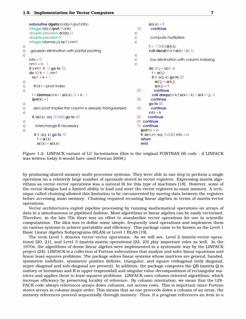
Figure 1.2: LINPACK variant of LU factorization (this is the original FORTRAN 66 code - if LINPACKwas written today it would have used Fortran 2008.)

by producing shared memory multi-processor systems. They were able in one step to perform a singleoperation on a relatively large number of operands stored in vector registers. Expressing matrix algo-rithms as vector-vector operations was a natural fit for this type of machines [18]. However, some ofthe vector designs had a limited ability to load and store the vector registers in main memory. A tech-nique called chaining allowed this limitation to be circumvented by moving data between the registersbefore accessing main memory. Chaining required recasting linear algebra in terms of matrix-vectoroperations.

Vector architectures exploit pipeline processing by running mathematical operations on arrays ofdata in a simultaneous or pipelined fashion. Most algorithms in linear algebra can be easily vectorized.Therefore, in the late 70s there was an effort to standardize vector operations for use in scientificcomputations. The idea was to define some simple, frequently used operations and implement themon various systems to achieve portability and efficiency. This package came to be known as the Level 1Basic Linear Algebra Subprograms (BLAS) or Level 1 BLAS [19].

The term Level 1 denotes vector-vector operations. As we will see, Level 2 (matrix-vector opera-tions) [20, 21], and Level 3 (matrix-matrix operations) [22, 23] play important roles as well. In the1970s, the algorithms of dense linear algebra were implemented in a systematic way by the LINPACKproject [24]. LINPACK is a collection of Fortran subroutines that analyze and solve linear equations andlinear least-squares problems. The package solves linear systems whose matrices are general, banded,symmetric indefinite, symmetric positive definite, triangular, and square tridiagonal (only diagonal,super-diagonal and sub-diagonal are present). In addition, the package computes the QR (matrix Q isunitary or hermitian and R is upper trapezoidal) and singular value decompositions of rectangular ma-trices and applies them to least-squares problems. LINPACK uses column-oriented algorithms, whichincrease efficiency by preserving locality of reference. By column orientation, we mean that the LIN-PACK code always references arrays down columns, not across rows. This is important since Fortranstores arrays in column-major order. This means that as one proceeds down a column of an array, thememory references proceed sequentially through memory. Thus, if a program references an item in a


particular block, the next reference is likely to be in the same block.The software in LINPACK was kept machine-independent partly through the introduction of the

Level 1 BLAS routines. Calling Level 1 BLAS did almost all of the computation. For each machine, theset of Level 1 BLAS would be implemented in a machine-specific manner to obtain high performance.The Level 1 BLAS subroutines DAXPY, DSCAL, and IDAMAX are used in the routine DGEFA.

It was presumed that the BLAS operations would be implemented in an efficient, machine-specificway suitable for the computer on which the subroutines were executed. On a vector computer, thiscould translate into a simple, single vector operation. This avoided leaving the optimization up to thecompiler and explicitly exposing a performance-critical operation.

In a sense, then, the beauty of the original code was regained with the use of a new vocabulary todescribe the algorithms: the BLAS. Over time, the BLAS became a widely adopted standard and weremost likely the first to enforce two key aspects of software: modularity and portability. Again, these aretaken for granted today, but at the time they were not. One could have the cake of compact algorithmrepresentation and eat it too, because the resulting Fortran code was portable.

Most algorithms in linear algebra can be easily vectorized. However, to gain the most out of sucharchitectures, simple vectorization is usually not enough. Some vector computers are limited by havingonly one path between memory and the vector registers. This creates a bottleneck if a program loadsa vector from memory, performs some arithmetic operations, and then stores the results. In orderto achieve top performance, the scope of the vectorization must be expanded to facilitate chainingoperations together and to minimize data movement, in addition to using vector operations. Recastingthe algorithms in terms of matrix-vector operations makes it easy for a vectorizing compiler to achievethese goals.

Thus, as computer architectures became more complex in the design of their memory hierarchies,it became necessary to increase the scope of the BLAS routines from Level 1 to Level 2 and Level 3.

1.6 Implementation on RISC Processors

RISC computers were introduced in the late 1980s and early 1990s. While their clock rates might havebeen comparable to those of the vector machines, the computing speed lagged behind due to their lackof vector registers. Another deficiency was their creation of a deep memory hierarchy with multiplelevels of cache memory to alleviate the scarcity of bandwidth that was, in turn, caused mostly by alimited number of memory banks. The eventual success of this architecture is commonly attributed tothe right price point and astonishing improvements in performance over time as predicted by Moore’sLaw [25]. With RISC computers, the linear algebra algorithms had to be redone yet again. This time,the formulations had to expose as many matrix-matrix operations as possible, which guaranteed goodcache reuse.

As mentioned before, the introduction in the late 1970s and early 1980s of vector machines broughtabout the development of another variant of algorithms for dense linear algebra. This variant wascentered on the multiplication of a matrix by a vector. These subroutines were meant to give improvedperformance over the dense linear algebra subroutines in LINPACK, which were based on Level 1BLAS. In the late 1980s and early 1990s, with the introduction of RISC-type microprocessors (the“killer micros”) and other machines with cache-type memories, we saw the development of LAPACK [26]Level 3 algorithms for dense linear algebra. A Level 3 code is typified by the main Level 3 BLAS, which,in this case, is matrix multiplication [27].

The original goal of the LAPACK project was to make the widely used LINPACK library run efficientlyon vector and shared-memory parallel processors. On these machines, LINPACK is inefficient becauseits memory access patterns disregard the multilayered memory hierarchies of the machines, therebyspending too much time moving data instead of doing useful floating-point operations. LAPACK ad-dresses this problem by reorganizing the algorithms to use block matrix operations, such as matrixmultiplication, in the innermost loops (see the paper by E. Anderson and J. Dongarra under ”FurtherReading”). These block operations can be optimized for each architecture to account for its memoryhierarchy, and so provide a transportable way to achieve high efficiency on diverse modern machines.

Here we use the term “transportable” instead of “portable” because, for fastest possible performance,LAPACK requires that highly optimized block matrix operations be implemented already on each ma-chine. In other words, the correctness of the code is portable, but high performance is not – if we limitourselves to a single Fortran source code.

1.6. Implementation on RISC Processors 9

SUBROUTINE DGETRF(M, N, A, LDA, IPIV, INFO)INTEGER INFO, LDA, M, NINTEGER IPIV( * )DOUBLE PRECISION A( LDA, * )DOUBLE PRECISION ONEPARAMETER ( ONE = 1.0D+0 )INTEGER I, IINFO, J, JB, NB

EXTERNAL DGEMM, DGETF2, DLASWP, DTRSMEXTERNAL XERBLAINTEGER ILAENVEXTERNAL ILAENVINTRINSIC MAX, MININFO = 0IF( M.LT.0 ) THEN

INFO = -1ELSE IF( N.LT.0 ) THEN

INFO = -2ELSE IF( LDA.LT.MAX( 1, M ) ) THEN

INFO = -4END IF

IF( INFO.NE.0 ) THEN

CALL XERBLA( ’DGETRF’, -INFO )RETURN

END IF

IF( M.EQ.0 .OR. N.EQ.0 ) RETURN

NB = ILAENV( 1, ’DGETRF’, ’ ’, M, N, -1, -1 )IF( NB.LE.1 .OR. NB.GE.MIN( M, N ) ) THEN

CALL DGETF2( M, N, A, LDA, IPIV, INFO )ELSE

DO 20 J = 1, MIN( M, N ), NBJB = MIN( MIN( M, N )-J+1, NB )

* Factor diagonal and subdiagonal blocks and test for exact* singularity.

CALL DGETF2( M-J+1, JB, A( J, J ), LDA, IPIV( J ), IINFO )* Adjust INFO and the pivot indices.

IF( INFO.EQ.0 .AND. IINFO.GT.0 ) INFO = IINFO + J - 1DO 10 I = J, MIN( M, J+JB-1 )

IPIV( I ) = J - 1 + IPIV( I )10 CONTINUE

* Apply interchanges to columns 1:J-1.CALL DLASWP( J-1, A, LDA, J, J+JB-1, IPIV, 1 )IF( J+JB.LE.N ) THEN

* Apply interchanges to columns J+JB:N.CALL DLASWP( N-J-JB+1, A(1, J+JB), LDA, J, J+JB-1, IPIV, 1 )

* Compute block row of U.CALL DTRSM( ’Left’, ’Lower’, ’No transpose’, ’Unit’,

JB,$ N-J-JB+1, ONE, A(J, J), LDA, A(J, J+JB), LDA )

IF( J+JB.LE.M ) THEN

* Update trailing submatrix.CALL DGEMM( ’No transpose’, ’No transpose’,

M-J-JB+1,$ N-J-JB+1, JB, -ONE, A(J+JB, J), LDA,$ A(J, J+JB), LDA, ONE, A(J+JB, J+JB), LDA )

END IF

END IF

20 CONTINUE

END IF

RETURN

END

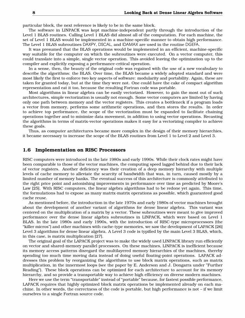
Figure 1.3: LAPACK’s LU factorization routine DGETRF (FORTRAN 77 coding.)

LAPACK can be regarded as a successor to LINPACK in terms of functionality, although it doesn’talways use the same function-calling sequences. As such a successor, LAPACK was a win for thescientific community because it could keep LINPACK’s functionality while getting improved use out ofnew hardware.

Most of the computational work in the algorithm from Figure 1.3 is contained in three routines:

• DGEMM - Matrix-matrix multiplication

• DTRSM - Triangular solve with multiple right hand sides

• DGETF2 - Unblocked LU factorization for operations within a block column

One of the key parameters in the algorithm is the block size, called NB here. If NB is too small ortoo large, poor performance can result-hence the importance of the ILAENV function, whose standardimplementation was meant to be replaced by a vendor implementation encapsulating machine- specificparameters upon installation of the LAPACK library. At any given point of the algorithm, NB columnsor rows are exposed to a well-optimized Level-3 BLAS. If NB is 1, the algorithm is equivalent in perfor-mance and memory access patterns to the LINPACK’s version.

Matrix-matrix operations offer the proper level of modularity for performance and transportabilityacross a wide range of computer architectures, including parallel systems with memory hierarchy. Thisenhanced performance is primarily due to a greater opportunity for reusing data. There are numerousways to accomplish this reuse of data to reduce memory traffic and to increase the ratio of floating-pointoperations to data movement through the memory hierarchy. This improvement can bring a three- toten-fold improvement in performance on modern computer architectures.

The jury is still out concerning the productivity of writing and reading the LAPACK code: how hardis it to generate the code from its mathematical description? The use of vector notation in LINPACK is


SUBROUTINE PDGETRF( M, N, A, IA, JA, DESCA, IPIV, INFO )INTEGER IA, INFO, JA, M, NINTEGER DESCA( * ), IPIV( * )DOUBLE PRECISION A( * )INTEGER BLOCK CYCLIC 2D, CSRC , CTXT , DLEN , DTYPE ,

$ LLD , MB , M , NB , N , RSRCPARAMETER ( BLOCK CYCLIC 2D = 1, DLEN = 9, DTYPE = 1,

$ CTXT = 2, M = 3, N = 4, MB = 5, NB = 6,$ RSRC = 7, CSRC = 8, LLD = 9 )DOUBLE PRECISION ONEPARAMETER ( ONE = 1.0D+0 )CHARACTER COLBTOP, COLCTOP, ROWBTOPINTEGER I, ICOFF, ICTXT, IINFO, IN, IROFF, J, JB, JN,

$ MN, MYCOL, MYROW, NPCOL, NPROWINTEGER IDUM1( 1 ), IDUM2( 1 )EXTERNAL BLACS GRIDINFO, CHK1MAT, IGAMN2D, PCHK1MAT,

$ PB TOPGET, PB TOPSET, PDGEMM, PDGETF2,$ PDLASWP, PDTRSM, PXERBLAINTEGER ICEILEXTERNAL ICEILINTRINSIC MIN, MOD

* Get grid parametersICTXT = DESCA( CTXT )CALL BLACS GRIDINFO( ICTXT, NPROW, NPCOL, MYROW, MYCOL )

* Test the input parametersINFO = 0IF( NPROW.EQ.-1 ) THEN

INFO = -(600+CTXT )ELSE

CALL CHK1MAT( M, 1, N, 2, IA, JA, DESCA, 6, INFO )IF( INFO.EQ.0 ) THEN

IROFF = MOD( IA-1, DESCA( MB ) )ICOFF = MOD( JA-1, DESCA( NB ) )IF( IROFF.NE.0 ) THEN

INFO = -4ELSE IF( ICOFF.NE.0 ) THEN

INFO = -5ELSE IF( DESCA( MB ).NE.DESCA( NB ) ) THEN

INFO = -(600+NB )END IF

END IFCALL PCHK1MAT( M, 1, N, 2, IA, JA, DESCA, 6, 0, IDUM1,

$ IDUM2, INFO )END IFIF( INFO.NE.0 ) THEN

CALL PXERBLA( ICTXT, ’PDGETRF’, -INFO )RETURN

END IF* Quick return if possible

IF( DESCA( M ).EQ.1 ) THENIPIV( 1 ) = 1RETURN

ELSE IF( M.EQ.0 .OR. N.EQ.0 ) THENRETURN

END IF* Split-ring topology for the communication along process rows

CALL PB TOPGET( ICTXT, ’Broadcast’, ’Rowwise’, ROWBTOP )CALL PB TOPGET( ICTXT, ’Broadcast’, ’Columnwise’, COLBTOP )CALL PB TOPGET( ICTXT, ’Combine’, ’Columnwise’, COLCTOP )CALL PB TOPSET( ICTXT, ’Broadcast’, ’Rowwise’, ROWBTOP )CALL PB TOPSET( ICTXT, ’Broadcast’, ’Columnwise’, COLBTOP )CALL PB TOPSET( ICTXT, ’Combine’, ’Columnwise’, COLCTOP )RETURNEND

CALL PB TOPSET( ICTXT, ’Broadcast’, ’Rowwise’, ’S-ring’ )CALL PB TOPSET( ICTXT, ’Broadcast’, ’Columnwise’, ’ ’ )CALL PB TOPSET( ICTXT, ’Combine’, ’Columnwise’, ’ ’ )

* Handle the first block of columns separatelyMN = MIN( M, N )IN = MIN( ICEIL( IA, DESCA( MB ) )*DESCA( MB ), IA+M-1 )JN = MIN( ICEIL( JA, DESCA( NB ) )*DESCA( NB ), JA+MN-1 )JB = JN - JA + 1


CALL PDGETF2( M, JB, A, IA, JA, DESCA, IPIV, INFO )IF( JB+1.LE.N ) THEN

* Apply interchanges to columns JN+1:JA+N-1.CALL PDLASWP( ’Forward’, ’Rows’, N-JB, A, IA, JN+1, DESCA,

$ IA, IN, IPIV )* Compute block row of U.

CALL PDTRSM( ’Left’, ’Lower’, ’No transpose’, ’Unit’, JB,$ N-JB, ONE, A, IA, JA, DESCA, A, IA, JN+1, DESCA )

IF( JB+1.LE.M ) THEN* Update trailing submatrix.

CALL PDGEMM( ’No transpose’, ’No transpose’, M-JB, N-JB,JB,

$ -ONE, A, IN+1, JA, DESCA, A, IA, JN+1, DESCA,$ ONE, A, IN+1, JN+1, DESCA )

END IFEND IF

* Loop over the remaining blocks of columns.DO 10 J = JN+1, JA+MN-1, DESCA( NB )

JB = MIN( MN-J+JA, DESCA( NB ) )I = IA + J - JA


CALL PDGETF2( M-J+JA, JB, A, I, J, DESCA, IPIV, IINFO )IF( INFO.EQ.0 .AND. IINFO.GT.0 )

$ INFO = IINFO + J - JA* Apply interchanges to columns JA:J-JA.

CALL PDLASWP( ’Forward’, ’Rowwise’, J-JA, A, IA, JA, DESCA,$ I, I+JB-1, IPIV )

IF( J-JA+JB+1.LE.N ) THEN* Apply interchanges to columns J+JB:JA+N-1.

CALL PDLASWP( ’Forward’, ’Rowwise’, N-J-JB+JA, A, IA, J+JB,$ DESCA, I, I+JB-1, IPIV )

* Compute block row of U.CALL PDTRSM( ’Left’, ’Lower’, ’No transpose’, ’Unit’, JB,

$ N-J-JB+JA, ONE, A, I, J, DESCA, A, I, J+JB,$ DESCA )

IF( J-JA+JB+1.LE.M ) THEN* Update trailing submatrix.

CALL PDGEMM( ’No transpose’, ’No transpose’, M-J-JB+JA,$ N-J-JB+JA, JB, -ONE, A, I+JB, J, DESCA, A,$ I, J+JB, DESCA, ONE, A, I+JB, J+JB, DESCA )

END IFEND IF

10 CONTINUEIF( INFO.EQ.0 )

$ INFO = MN + 1CALL IGAMN2D( ICTXT, ’Rowwise’, ’ ’, 1, 1, INFO, 1, IDUM1, IDUM2,

$ -1, -1, MYCOL )IF( INFO.EQ.MN+1 )

$ INFO = 0CALL PB TOPSET( ICTXT, ’Broadcast’, ’Rowwise’, ROWBTOP )CALL PB TOPSET( ICTXT, ’Broadcast’, ’Columnwise’, COLBTOP )CALL PB TOPSET( ICTXT, ’Combine’, ’Columnwise’, COLCTOP )RETURNEND

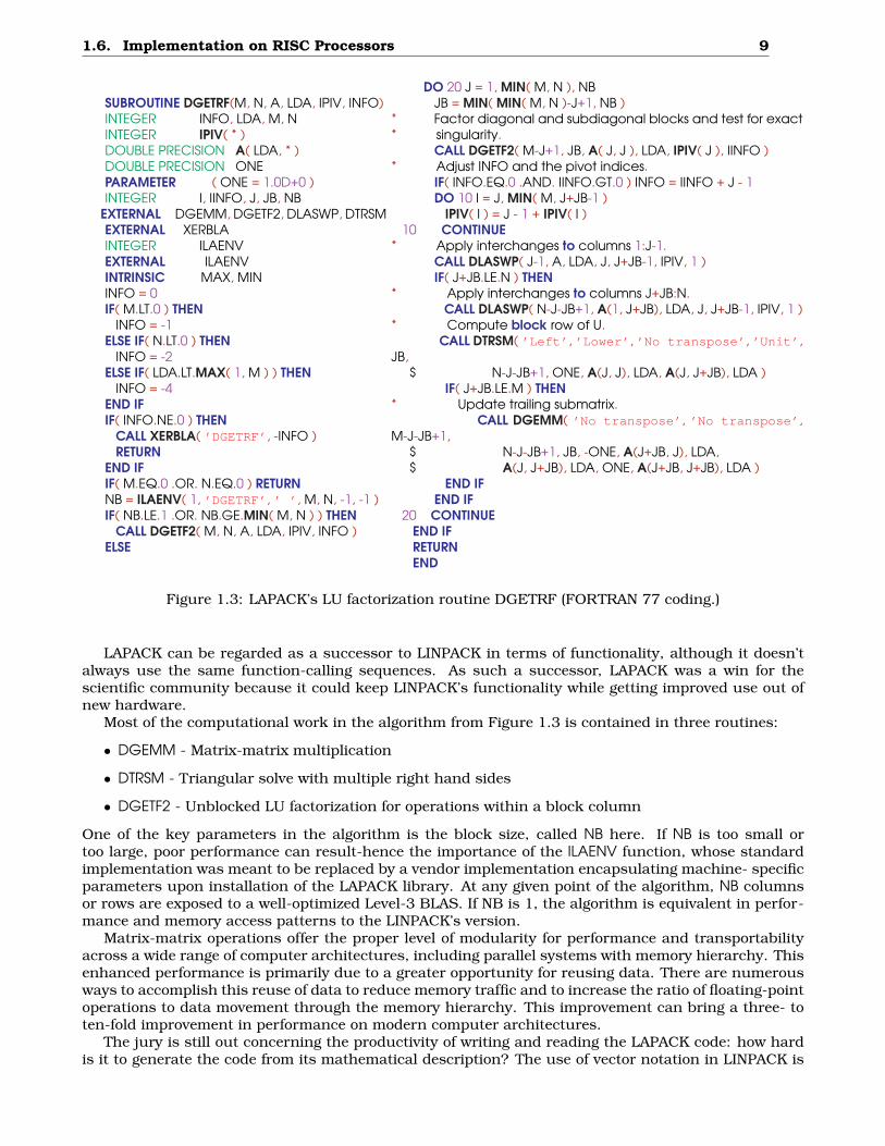
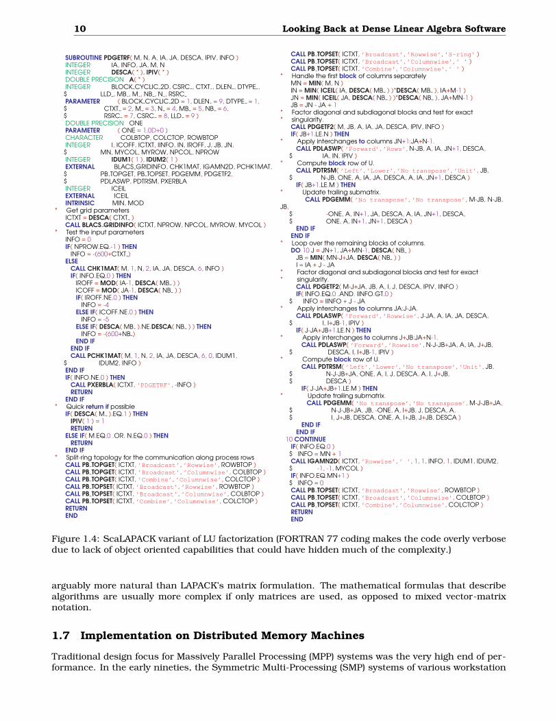
Figure 1.4: ScaLAPACK variant of LU factorization (FORTRAN 77 coding makes the code overly verbosedue to lack of object oriented capabilities that could have hidden much of the complexity.)

arguably more natural than LAPACK’s matrix formulation. The mathematical formulas that describealgorithms are usually more complex if only matrices are used, as opposed to mixed vector-matrixnotation.

1.7 Implementation on Distributed Memory Machines

Traditional design focus for Massively Parallel Processing (MPP) systems was the very high end of per-formance. In the early nineties, the Symmetric Multi-Processing (SMP) systems of various workstation

1.7. Implementation on Distributed Memory Machines 11

manufacturers as well as the IBM SP series, which targeted the lower and medium market segments,gained great popularity. Their price/performance ratios were better due to the missing overhead in thedesign for support of the very large configurations and due to cost advantages of the larger productionnumbers. Due to the vertical integration of performance it was no longer economically feasible to pro-duce and focus on the highest end of computing power alone. The design focus for new systems shiftedto the market of medium performance systems.

The acceptance of MPP systems not only for engineering applications but also for new commercialapplications especially for database applications emphasized different criteria for market success suchas the stability of the system, continuity of the manufacturer and price/performance. Success in com-mercial environments became a new important requirement for a successful supercomputer businesstowards the end of the nineties. Due to these factors and the consolidation in the number of vendorsin the market, hierarchical systems built with components designed for the broader commercial mar-ket did replace homogeneous systems at the very high end of performance. The marketplace adoptedclusters of SMPs readily, while academic research focused on clusters of workstations and PCs.

At the end of the nineties clusters were common in academia but mostly as research objects andnot primarily as general purpose computing platforms for applications. Most of these clusters were ofcomparable small scale and as a result the November 1999 edition of the TOP500 [28] listed only sevencluster systems. This changed dramatically as industrial and commercial customers started deployingclusters as soon as applications with less stringent communication requirements permitted them totake advantage of the better price/performance ratio – roughly an order of magnitude of commoditybased clusters. At the same time, all major vendors in the HPC market started selling this type ofcluster to their customer base. In November 2004, clusters were the dominant architectures in theTOP500 with 294 systems at all levels of performance. Companies such as IBM and Hewlett-Packardsell the majority of these clusters and a large number of them are installed at commercial and industrialcustomers.

In the early 2000s, clusters build with off-the-shelf components gained more and more attentionnot only as academic research object but also computing platforms with end-users of HPC computingsystems. By 2004, these groups of clusters represent the majority of new systems on the TOP500 ina broad range of application areas. One major consequence of this trend was the rapid rise in theutilization of Intel processors in HPC systems. While virtually absent in the high end at the beginningof the decade, Intel processors are now used in the majority of HPC systems. Clusters in the ninetieswere mostly self-made system designed and built by small groups of dedicated scientist or applicationexperts. This changed rapidly as soon as the market for clusters based on PC technology matured.Nowadays, the large majority of TOP500-class clusters are manufactured and integrated by either a fewtraditional large HPC manufacturers such as IBM or Hewlett-Packard or numerous small, specializedintegrators of such systems.

In addition, there still is generally a large difference in the usage of clusters and their more inte-grated counterparts: clusters are mostly used for capacity computing while the integrated machinesprimarily are used for capability computing. The largest supercomputers are used for capability orturnaround computing where the maximum processing power is applied to a single problem. Thegoal is to solve a larger problem, or to solve a single problem in a shorter period of time. Capabilitycomputing enables the solution of problems that cannot otherwise be solved in a reasonable period oftime (for example, by moving from a 2D to a 3D simulation, using finer grids, or using more realisticmodels). Capability computing also enables the solution of problems with real-time constraints (e.g.,predicting weather). The main figure of merit is time to solution. Smaller or cheaper systems are usedfor capacity computing, where smaller problems are solved. Capacity computing can be used to enableparametric studies or to explore design alternatives; it is often needed to prepare for more expensiveruns on capability systems. Capacity systems will often run several jobs simultaneously. The mainfigure of merit is sustained performance per unit cost. Traditionally, vendors of large supercomputersystems have learned to provide for the capacity mode of operation as the precious resources of theirsystems were required to be used as effectively as possible. By contrast, Beowulf clusters are mostlyoperated through the Linux operating system (a small minority using Microsoft Windows) where theseoperating systems either lack the tools or these tools are relatively immature to use a cluster effectivelyfor capability computing. However, as clusters become on average both larger and more stable in termsof continuous operation, there is a trend to use them also as computational capability servers.

There are a number of choices of communication networks available in clusters. Of course 100 Mb/s


Ethernet or Gigabit Ethernet is always possible, which is attractive for economic reasons, but it hasthe drawback of a high latency (∼ 100µs) – the time it takes to send the shortest message. Alternatively,there are, for instance, networks that operate from user space, like Myrinet, Infiniband. The networkspeeds as shown by these networks are more or less on par with some integrated parallel systems. So,possibly apart from the speed of the processors and of the software that is provided by the vendorsof traditional integrated supercomputers, the distinction between clusters and the class of customcapability machines becomes rather small and will, without a doubt, decrease further in the comingyears. And the advances of the Ethernet standard into the 100 Gb/s territory with latencies well below10 µs make it even more so.

LAPACK was designed to be highly efficient on vector processors, high-performance “superscalar”workstations, and shared-memory multiprocessors. LAPACK can also be used satisfactorily on all typesof scalar machines (PCs, workstations, and mainframes). However, LAPACK in its present form is lesslikely to give good performance on other types of parallel architectures – for example, massively par-allel Single Instruction Multiple Data (SIMD) machines, or Multiple Instruction Multiple Data (MIMD)distributed-memory machines. The ScaLAPACK effort was intended to adapt LAPACK to these newarchitectures.

Like LAPACK, the ScaLAPACK routines are based on block-partitioned algorithms in order to min-imize the frequency of data movement between different levels of the memory hierarchy. The funda-mental building blocks of the ScaLAPACK library are distributed-memory versions of the Level-2 andLevel-3 BLAS [29], and a set of Basic Linear Algebra Communication Subprograms (BLACS) [30] forcommunication tasks that arise frequently in parallel linear algebra computations. In the ScaLAPACKroutines, all interprocessor communication occurs within the distributed BLAS and the BLACS, so thesource code of the top software layer of ScaLAPACK looks very similar to that of LAPACK. The similaritymay be observed by comparing Figures 1.3 and 1.4.

In order to simplify the design of ScaLAPACK, and because the BLAS have proven to be very usefultools outside LAPACK, we chose to build a Parallel BLAS, or PBLAS [29], whose interface is as similarto the BLAS as possible. This decision has permitted the ScaLAPACK code to be quite similar, andsometimes nearly identical, to the analogous LAPACK code.

It was our aim that the PBLAS would provide a distributed memory standard, just as the BLASprovided a shared memory standard. This would simplify and encourage the development of highperformance and portable parallel numerical software, as well as providing manufacturers with just asmall set of routines to be optimized. The acceptance of the PBLAS requires reasonable compromisesbetween competing goals of functionality and simplicity.

The PBLAS operate on matrices distributed in a two-dimensional block cyclic layout. Because sucha data layout requires many parameters to fully describe the distributed matrix, we have chosen amore object-oriented approach and encapsulated these parameters in an integer array called an arraydescriptor. An array descriptor includes:

• The descriptor type

• The BLACS context (a virtual space for messages that is created to avoid collisions between logi-cally distinct messages)

• The number of rows in the distributed matrix

• The number of columns in the distributed matrix

• The row block size

• The column block size

• The process row over which the first row of the matrix is distributed

• The process column over which the first column of the matrix is distributed

• The leading dimension of the local array storing the local blocks

By using this descriptor, a call to a PBLAS routine is very similar to a call to the corresponding BLASroutine:CALL DGEMM ( TRANSA, TRANSB, M, N, K, ALPHA, A( IA, JA ), LDA, B( IB, JB ), LDB, BETA, C( IC, JC ), LDC )

1.8. Shared Memory Implementation 13

CALL PDGEMM( TRANSA, TRANSB, M, N, K, ALPHA, A, IA, JA, DESC A, B, JB, DESC B, BETA, C, IC, JC, DESC C)DGEMM computes C = BETA × C + ALPHA × op( A ) × op( B ), where op(A) is either A or its transposedepending on TRANSA, op(B) is similar, op(A) is M-by-K, and op(B) is K-by-N. PDGEMM is the same,with the exception of the way submatrices are specified. To pass the submatrix starting at A(IA,JA) toDGEMM, for example, the actual argument corresponding to the formal argument A is simply A(IA,JA).PDGEMM, on the other hand, needs to understand the global storage scheme of A to extract the correctsubmatrix, so IA and JA must be passed in separately.

DESC A is the array descriptor for A. The parameters describing the matrix operands B and C areanalogous to those describing A. In a truly object-oriented environment, matrices and DESC A wouldbe synonymous. However, this would require language support and detract from portability.

Using message passing and scalable algorithms from the ScaLAPACK library makes it possible tofactor matrices of arbitrarily increasing size, given machines with more processors. By design, thelibrary computes more than it communicates, so for the most part, data stay locally for processing andtravels only occasionally across the interconnect network.

But the number and types of messages exchanged between processors can sometimes be hardto manage. The context associated with every distributed matrix lets implementations use separate“universes” for message passing. The use of separate communication contexts by distinct libraries (ordistinct library invocations) such as the PBLAS insulates communication internal to the library fromexternal communication. When more than one descriptor array is present in the argument list of aroutine in the PBLAS, the individual BLACS context entries must be equal. In other words, the PBLASdo not perform “inter-context” operations.

In the performance sense, ScaLAPACK did to LAPACK what LAPACK did to LINPACK: it broadenedthe range of hardware where LU factorization (and other codes) could run efficiently. In terms of codeelegance, the ScaLAPACK’s changes were much more drastic: the same mathematical operation nowrequired large amounts of tedious work. Both the users and the library writers were now forced intoexplicitly controlling data storage intricacies, because data locality became paramount for performance.The victim was the readability of the code, despite efforts to modularize the code according to the bestsoftware engineering practices of the day.

1.8 Shared Memory Implementation

The advent of multi-core processorss brought about a fundamental shift in the way software is pro-duced even though comparisons have been brought up with the established coding techniques fromSMPs. Rather elaborating the differences we will focus on how most of software had to be adjusted forSMPs with a special focus on dense linear algebra. The good news is that LAPACK’s LU factorizationruns on a multi-core system and can even deliver a modest increase of performance if multi-threadedBLAS are used. In technical terms, this is the Block Synchronous Processing (BSP) model [31] model ofparallel computation: each call to BLAS (from a single main thread) forks a suitable number of threads(parallel units of executions that share memory and are often scheduled by the operating system),which perform the work on each core and then join the main thread of computation. This is also calleda fork-join model and it implies a synchronization point at each join operation.

The bad news is that the LAPACK’s fork-join algorithm gravely impairs scalability even on smallmulti-core computers that do not have the memory systems available in SMP systems. The inherentscalability flaw is the heavy synchronization in the fork-join model:only a single thread is allowed toperform the significant computation that occupies the critical section of the code, leaving other threadsidle. That results in lock-step execution: all threads have to wait for the slowest one among them. Italso prevents hiding of inherently sequential portions of the code behind parallel ones. In other words,the threads are forced to perform the same operation on different data. If there is not enough data forsome threads, they will have to stay idle and wait for the rest of the threads that perform useful workon their data. Clearly, another version of the LU algorithm is needed such that would allow threads tostay busy all the time by possibly making them perform different operations during some portion of theexecution.

The multithreaded version of the algorithm recognizes the existence of a so-called critical path inthe algorithm: a portion of the code whose execution depends on previous calculations and can block


voidSMP dgetrf(int n, double *a, int lda, int *ipiv, int NB,

int tid, int tsize, int *pready, ptm *mtx, ptc *cnd) {int pcnt, pfctr, ufrom, uto, ifrom, p;double *pa = a, *pl, *pf, *lp;

pcnt = n / NB; /* number of panels */

/* first panel that should be factored by this thread after

* the very first panel (number 0) gets factored */

pfctr = tid + (tid ? 0 : tsize);

/* this is a pointer to the last panel */

lp = a + (size t)(n - NB) * (size t)lda;

/* for each panel (that is used as source of updates) */

for (ufrom = 0; ufrom < pcnt;ufrom++, pa += NB * (size t)(lda + 1)){

p = ufrom * NB; /* column number */

/* if the panel to be used for updates has not been

* factored yet; ’ipiv’ does not be consulted, but it is

* to possibly avoid accesses to ’pready’ */

if (! ipiv[p + NB - 1] || ! pready[ufrom]) {/* if this is this thread’s panel */

if (ufrom % tsize == tid) {pfactor(n-p, NB, pa, lda, ipiv+p, pready, ufrom, mtx,

cnd);

/* if this is not the last panel */

} else if (ufrom < pcnt - 1) {LOCK( mtx );while (! pready[ufrom]) { WAIT( cnd, mtx ); }UNLOCK( mtx );

}}

/* for each panel to be updated */

for (uto = first panel to update( ufrom, tid, tsize );uto < pcnt; uto += tsize) {

/* if there are still panels to factor by this thread and

* preceding panel has been factored; test to ’ipiv’

* could be skipped but is in there to decrease number

* of accesses to ’pready’ */

if (pfctr < pcnt && ipiv[pfctr*NB-1] &&pready[pfctr-1]) {

/* for each panel that has to (still) update panel

* ’pfctr’ */

for (ifrom = ufrom + (uto>pfctr ? 1 : 0); ifrom < pfctr;ifrom++) {

p = ifrom * NB;pl = a + (size t)p * (size t)(lda + 1);pf = pl + (size t)(pfctr - ifrom) * (size t)NB * lda;pupdate( n - p, NB, pl, pf, lda, p, ipiv, lp );

}p = pfctr * NB;pl = a + (size t)p * (size t)(lda + 1);

pfactor(n-p, NB, pl, lda, ipiv+p, pready, pfctr, mtx,cnd);

pfctr += tsize; /* move to this thread’s next panel */

}/* if panel ’uto’ hasn’t been factored (if it was, it

* certainly has been updated, so no update is

* necessary) */

if (uto > pfctr || ! ipiv[uto * NB]) {p = ufrom * NB;pf = pa + (uto - ufrom) * (size t)NB * lda;pupdate( n - p, NB, pa, pf, lda, p, ipiv, lp );

}}

}}

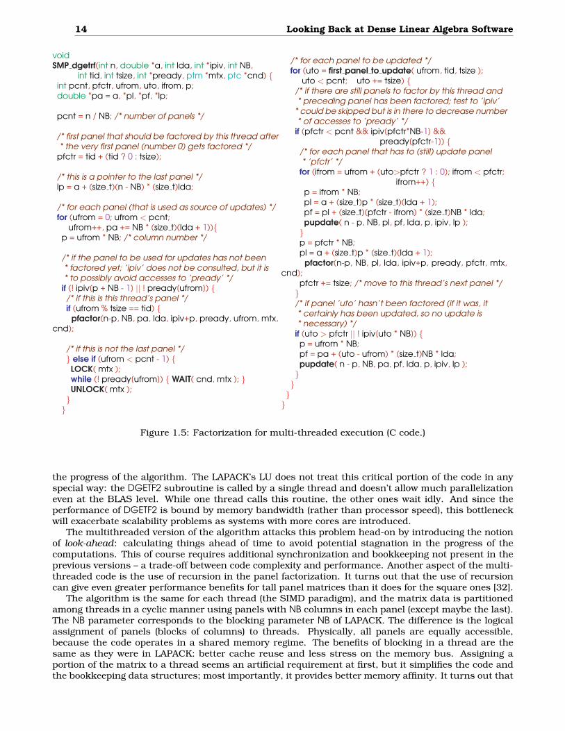
Figure 1.5: Factorization for multi-threaded execution (C code.)

the progress of the algorithm. The LAPACK’s LU does not treat this critical portion of the code in anyspecial way: the DGETF2 subroutine is called by a single thread and doesn’t allow much parallelizationeven at the BLAS level. While one thread calls this routine, the other ones wait idly. And since theperformance of DGETF2 is bound by memory bandwidth (rather than processor speed), this bottleneckwill exacerbate scalability problems as systems with more cores are introduced.

The multithreaded version of the algorithm attacks this problem head-on by introducing the notionof look-ahead: calculating things ahead of time to avoid potential stagnation in the progress of thecomputations. This of course requires additional synchronization and bookkeeping not present in theprevious versions – a trade-off between code complexity and performance. Another aspect of the multi-threaded code is the use of recursion in the panel factorization. It turns out that the use of recursioncan give even greater performance benefits for tall panel matrices than it does for the square ones [32].

The algorithm is the same for each thread (the SIMD paradigm), and the matrix data is partitionedamong threads in a cyclic manner using panels with NB columns in each panel (except maybe the last).The NB parameter corresponds to the blocking parameter NB of LAPACK. The difference is the logicalassignment of panels (blocks of columns) to threads. Physically, all panels are equally accessible,because the code operates in a shared memory regime. The benefits of blocking in a thread are thesame as they were in LAPACK: better cache reuse and less stress on the memory bus. Assigning aportion of the matrix to a thread seems an artificial requirement at first, but it simplifies the code andthe bookkeeping data structures; most importantly, it provides better memory affinity. It turns out that

1.9. Multicore Implementations 15

multi-core chips are not symmetric in terms of memory access bandwidth, so minimizing the numberof reassignments of memory pages to cores directly benefits performance.

The standard components of LU factorization are represented by the pfactor() and pupdate() func-tions in Figure 1.5. As one might expect, the former factors a panel, whereas the latter updates a panelusing one of the previously factored panels.

The main loop makes each thread iterate over each panel in turn. If necessary, the panel is factoredby the owner thread while other threads wait (if they happen to need this panel for their updates).

The look-ahead logic is inside the nested loop (prefaced by the comment for each panel to be updated)that replaces DGEMM or PDGEMM from previous algorithms. Before each thread updates one of itspanels, it checks whether its already feasible to factor its first unfactored panel. This minimizes thenumber of times the threads have to wait because each thread constantly attempts to eliminate thepotential bottleneck.

As was the case for ScaLAPACK, the multithreaded version detracts from the inherent elegance ofthe LAPACKs version. Also in the same spirit, performance is the main culprit: LAPACKs code willnot run efficiently on machines with ever-increasing numbers of cores. Explicit control of executionthreads at the LAPACK level rather than the BLAS level is critical: parallelism cannot be encapsulatedin a library call. The only good news is that the code is not as complicated as ScaLAPACKs, and efficientBLAS can still be put to a good use.

1.9 Multicore Implementations

The multicore processors do not resemble the SMP systems of the past, nor do they resemble distributedmemory systems. In comparison to SMPs, multicores are much more starved for memory due to thefast increase in the number of cores, which is not followed by a proportional increase in bandwidth.Owing to that, data access locality is of much higher importance in case of multicores. At the sametime, they do follow to a large extent the memory model where the main memory serves as a central(not distributed) repository for data. For those reasons, the best performing algorithms or multicoreshappen to be parallel versions of what used to be know as “out of core” algorithms (algorithms developedin the past for situations where data does not fit in the main memory and has to be explicitly movedbetween the memory and the disc).

In dense linear algebra, the Tile Algorithms are direct descendants of ”out of core” algorithms. TheTile Algorithms are based on the idea of processing the matrix by square submatrices, referred to astiles, of relatively small size. This makes the operation efficient in terms of cache and TLB use. TheCholesky factorization lends itself readily to tile formulation, however the same is not true for the LUand QR factorizations. The tile algorithms for them are constructed by factorizing the diagonal tile firstand then incrementally updating the factorization using the entries below the diagonal tile. This is avery well known concept that dates back to the work of Gauss. The idea was initially used to build“out-of-core” algorithms and recently rediscovered as a very efficient method for implementing linearalgebra operations on multicore processors. It is crucial to note that the technique of processing thematrix by square tiles yields satisfactory performance only when accompanied by data organizationbased on square tiles. The layout is referred to as Square Block layout or, simply, Tile Layout.

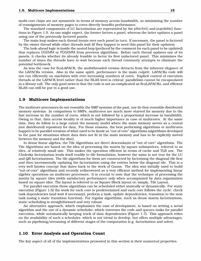
For parallel execution those algorithms can be scheduled either statically or dynamically. For staticexecution (Figure 1.6) the work for each core is predetermined and each core follows the cycle: checktask dependencies (and wait if necessary), perform a task, update dependencies, transition to the nexttask (using a static transition function). For regular algorithms, such as dense matrix factorizations,static scheduling is straightforward and very robust.

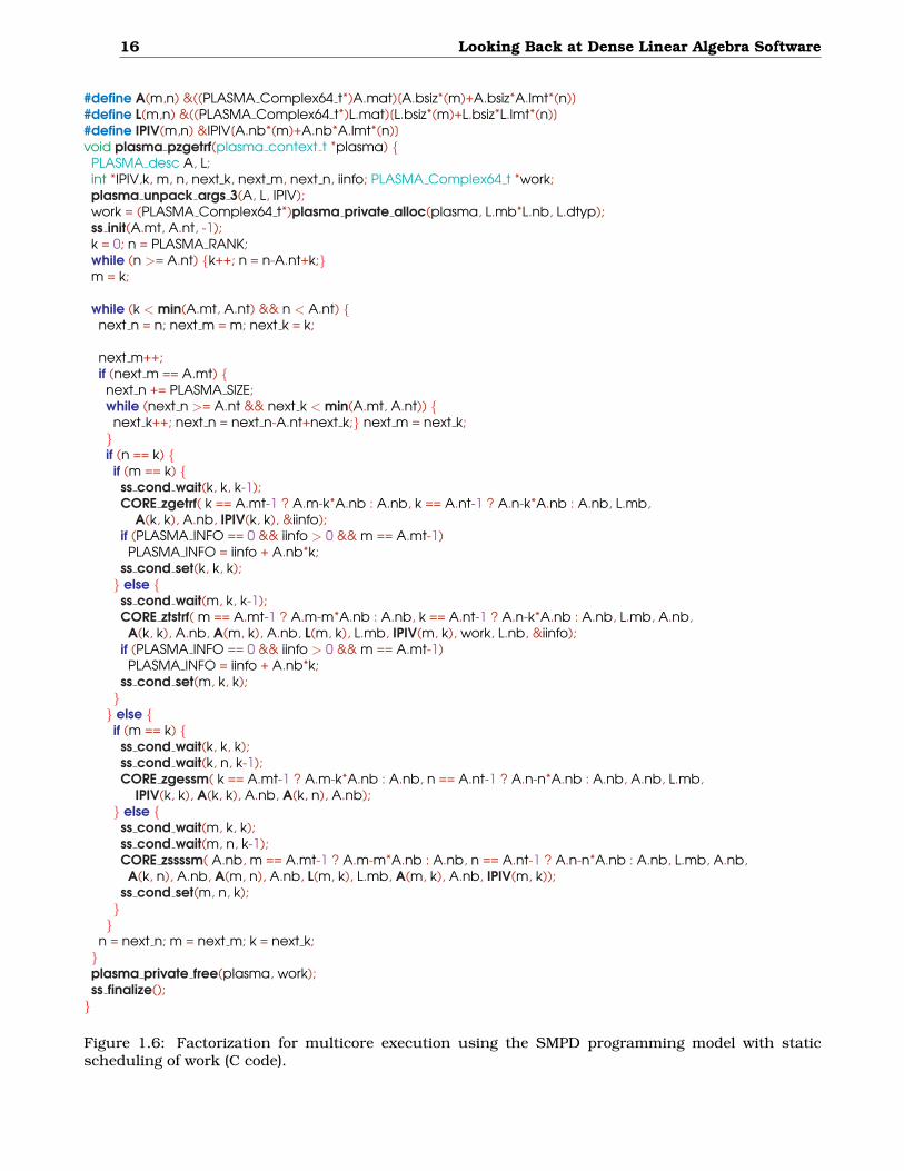
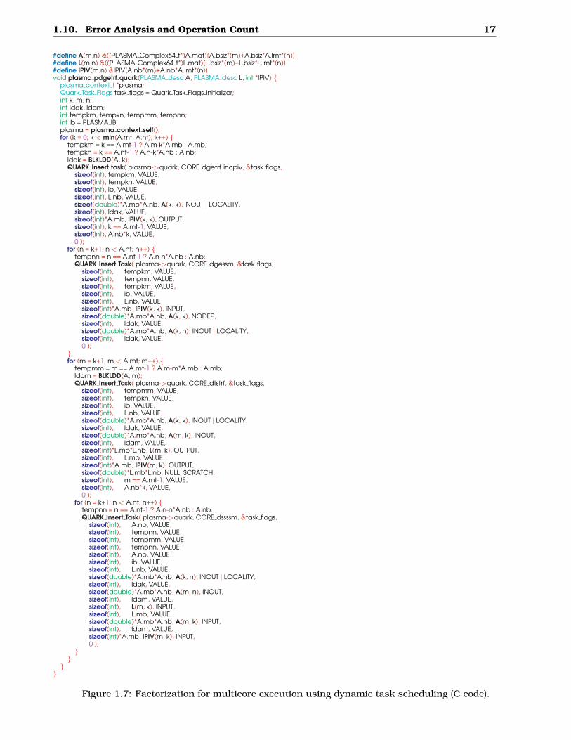
An alternative approach, which emphasizes the ease of development, is based on writing a serialalgorithm and the use of a dynamic scheduler, which traverses the code and queues tasks for parallelexecution, while automatically keeping track of data dependencies (Figure 1.7). This approach relieson the availability of such a scheduler, which is not trivial to develop, but offers multiple advantages,such as pipelining/streaming of different stages of the computation (e.g. factorization and solve).

1.10 Error Analysis and Operation Count

The key aspect of all of the implementations presented in this section is their numerical properties.


#define A(m,n) &((PLASMA Complex64 t*)A.mat)[A.bsiz*(m)+A.bsiz*A.lmt*(n)]#define L(m,n) &((PLASMA Complex64 t*)L.mat)[L.bsiz*(m)+L.bsiz*L.lmt*(n)]#define IPIV(m,n) &IPIV[A.nb*(m)+A.nb*A.lmt*(n)]void plasma pzgetrf(plasma context t *plasma) {

PLASMA desc A, L;int *IPIV,k, m, n, next k, next m, next n, iinfo; PLASMA Complex64 t *work;plasma unpack args 3(A, L, IPIV);work = (PLASMA Complex64 t*)plasma private alloc(plasma, L.mb*L.nb, L.dtyp);ss init(A.mt, A.nt, -1);k = 0; n = PLASMA RANK;while (n >= A.nt) {k++; n = n-A.nt+k;}m = k;

while (k < min(A.mt, A.nt) && n < A.nt) {next n = n; next m = m; next k = k;

next m++;if (next m == A.mt) {

next n += PLASMA SIZE;while (next n >= A.nt && next k < min(A.mt, A.nt)) {

next k++; next n = next n-A.nt+next k;} next m = next k;}if (n == k) {if (m == k) {ss cond wait(k, k, k-1);CORE zgetrf( k == A.mt-1 ? A.m-k*A.nb : A.nb, k == A.nt-1 ? A.n-k*A.nb : A.nb, L.mb,

A(k, k), A.nb, IPIV(k, k), &iinfo);if (PLASMA INFO == 0 && iinfo > 0 && m == A.mt-1)

PLASMA INFO = iinfo + A.nb*k;ss cond set(k, k, k);

} else {ss cond wait(m, k, k-1);CORE ztstrf( m == A.mt-1 ? A.m-m*A.nb : A.nb, k == A.nt-1 ? A.n-k*A.nb : A.nb, L.mb, A.nb,A(k, k), A.nb, A(m, k), A.nb, L(m, k), L.mb, IPIV(m, k), work, L.nb, &iinfo);

if (PLASMA INFO == 0 && iinfo > 0 && m == A.mt-1)PLASMA INFO = iinfo + A.nb*k;

ss cond set(m, k, k);}

} else {if (m == k) {ss cond wait(k, k, k);ss cond wait(k, n, k-1);CORE zgessm( k == A.mt-1 ? A.m-k*A.nb : A.nb, n == A.nt-1 ? A.n-n*A.nb : A.nb, A.nb, L.mb,

IPIV(k, k), A(k, k), A.nb, A(k, n), A.nb);} else {ss cond wait(m, k, k);ss cond wait(m, n, k-1);CORE zssssm( A.nb, m == A.mt-1 ? A.m-m*A.nb : A.nb, n == A.nt-1 ? A.n-n*A.nb : A.nb, L.mb, A.nb,A(k, n), A.nb, A(m, n), A.nb, L(m, k), L.mb, A(m, k), A.nb, IPIV(m, k));

ss cond set(m, n, k);}

}n = next n; m = next m; k = next k;

}plasma private free(plasma, work);ss finalize();

}

Figure 1.6: Factorization for multicore execution using the SMPD programming model with staticscheduling of work (C code).

1.10. Error Analysis and Operation Count 17

#define A(m,n) &((PLASMA Complex64 t*)A.mat)[A.bsiz*(m)+A.bsiz*A.lmt*(n)]#define L(m,n) &((PLASMA Complex64 t*)L.mat)[L.bsiz*(m)+L.bsiz*L.lmt*(n)]#define IPIV(m,n) &IPIV[A.nb*(m)+A.nb*A.lmt*(n)]void plasma pdgetrf quark(PLASMA desc A, PLASMA desc L, int *IPIV) {

plasma context t *plasma;Quark Task Flags task flags = Quark Task Flags Initializer;int k, m, n;int ldak, ldam;int tempkm, tempkn, tempmm, tempnn;int ib = PLASMA IB;plasma = plasma context self();for (k = 0; k < min(A.mt, A.nt); k++) {

tempkm = k == A.mt-1 ? A.m-k*A.mb : A.mb;tempkn = k == A.nt-1 ? A.n-k*A.nb : A.nb;ldak = BLKLDD(A, k);QUARK Insert task( plasma->quark, CORE dgetrf incpiv, &task flags,

sizeof(int), tempkm, VALUE,sizeof(int), tempkn, VALUE,sizeof(int), ib, VALUE,sizeof(int), L.nb, VALUE,sizeof(double)*A.mb*A.nb, A(k, k), INOUT | LOCALITY,sizeof(int), ldak, VALUE,sizeof(int)*A.mb, IPIV(k, k), OUTPUT,sizeof(int), k == A.mt-1, VALUE,sizeof(int), A.nb*k, VALUE,0 );

for (n = k+1; n < A.nt; n++) {tempnn = n == A.nt-1 ? A.n-n*A.nb : A.nb;QUARK Insert Task( plasma->quark, CORE dgessm, &task flags,

sizeof(int), tempkm, VALUE,sizeof(int), tempnn, VALUE,sizeof(int), tempkm, VALUE,sizeof(int), ib, VALUE,sizeof(int), L.nb, VALUE,sizeof(int)*A.mb, IPIV(k, k), INPUT,sizeof(double)*A.mb*A.nb, A(k, k), NODEP,sizeof(int), ldak, VALUE,sizeof(double)*A.mb*A.nb, A(k, n), INOUT | LOCALITY,sizeof(int), ldak, VALUE,0 );

}for (m = k+1; m < A.mt; m++) {

tempmm = m == A.mt-1 ? A.m-m*A.mb : A.mb;ldam = BLKLDD(A, m);QUARK Insert Task( plasma->quark, CORE dtstrf, &task flags,

sizeof(int), tempmm, VALUE,sizeof(int), tempkn, VALUE,sizeof(int), ib, VALUE,sizeof(int), L.nb, VALUE,sizeof(double)*A.mb*A.nb, A(k, k), INOUT | LOCALITY,sizeof(int), ldak, VALUE,sizeof(double)*A.mb*A.nb, A(m, k), INOUT,sizeof(int), ldam, VALUE,sizeof(int)*L.mb*L.nb, L(m, k), OUTPUT,sizeof(int), L.mb, VALUE,sizeof(int)*A.mb, IPIV(m, k), OUTPUT,sizeof(double)*L.mb*L.nb, NULL, SCRATCH,sizeof(int), m == A.mt-1, VALUE,sizeof(int), A.nb*k, VALUE,0 );

for (n = k+1; n < A.nt; n++) {tempnn = n == A.nt-1 ? A.n-n*A.nb : A.nb;QUARK Insert Task( plasma->quark, CORE dssssm, &task flags,

sizeof(int), A.nb, VALUE,sizeof(int), tempnn, VALUE,sizeof(int), tempmm, VALUE,sizeof(int), tempnn, VALUE,sizeof(int), A.nb, VALUE,sizeof(int), ib, VALUE,sizeof(int), L.nb, VALUE,sizeof(double)*A.mb*A.nb, A(k, n), INOUT | LOCALITY,sizeof(int), ldak, VALUE,sizeof(double)*A.mb*A.nb, A(m, n), INOUT,sizeof(int), ldam, VALUE,sizeof(int), L(m, k), INPUT,sizeof(int), L.mb, VALUE,sizeof(double)*A.mb*A.nb, A(m, k), INPUT,sizeof(int), ldam, VALUE,sizeof(int)*A.mb, IPIV(m, k), INPUT,0 );

}}

}}

Figure 1.7: Factorization for multicore execution using dynamic task scheduling (C code).


It is acceptable to forgo elegance in order to gain performance. But numerical stability is of vitalimportance and cannot be sacrificed, because it is an inherent part of the algorithms correctness.While these are serious considerations, there is some consolation to follow. It may be surprising tosome readers that all of the algorithms presented are the same, even though its virtually impossibleto make each excerpt of code produce exactly the same output for exactly the same inputs. Thefundamental reason for this are the vagaries of the floating-point arithmetic in finite precision as itis implemented in virtually all hardware. In essence, only a slight change in the order in which thefloating-point operations are performed causes a change in the result: the change is on the order of the,so called, machine precision. Machine precision comes from the number of decimal digits representedin the floating-point format: for double precision there are 15 digits and so the machine precision isabout 10−15. LINPACK and LAPACK perform the operations in different order because the latter mergesthe updates into a single call to BLAS. And even though ScaLAPACK merges the updates in a similarfashion as LAPACK does, the former performs its operations only on the local portion of the matrixwhereas the latter treats the matrix as a single piece quantity. In other words, when LAPACK makesa single update operation, ScaLAPACK could make as many as there are processors involved in thecomputation.

When it comes to repeatability of results, the vagaries of floating-point representation may be cap-tured in a rigorous way by error bounds. One way of expressing the numerical robustness of theprevious algorithms is with the following formula:

‖Ax−b‖‖A‖

≤ ‖x− x‖ ≤ ‖A−1‖‖Ax−b‖ (1.6)

where the error vector x− x is the difference between the computed solution x and the correct solutionx, and Ax−b is a so-called “residual”. The previous formula basically says that the size of the error (theparallel bars surrounding a value indicate a norm – a measure of absolute size) is as small as warrantedby the quality of the matrix A. Therefore, if the matrix is close to being singular in numerical sense(some entries are small with respect to machine precision and the condition number of the matrix andso they might be considered to be zero) the algorithms will not give an accurate answer. But otherwise,a relatively good quality of the result may be expected.

Another feature that is common to all the versions presented is the operation count: they all per-form O(2/3n3) floating-point multiplications and/or additions. The order of these operations is whatdifferentiates them. There exist algorithms that increase the amount of floating-point work to save onmemory traffic or network transfers (especially for distributed-memory parallel algorithms.) But be-cause the algorithms shown in this chapter have the same operation count, it is valid to compare themfor performance. The computational rate (number of floating-point operations per second) may be usedinstead of the time taken to solve the problem, provided that the matrix size is the same. But comparingcomputational rates is sometimes better because it allows a comparison of algorithms when the matrixsizes differ. For example, a sequential algorithm on a single processor can be directly compared with aparallel one working on a large cluster on a much bigger matrix.

1.11 Concluding Remarks and Future Directions

In this chapter we have looked at the evolution of the design of a simple but important algorithm incomputational science. The changes over the past 30 years have been necessary to follow the leadof the advances in computer architectures. In some cases these changes have been simple, suchas interchanging loops. In other cases, they have been as complex as the introduction of recursionand look-ahead computations. In each case, however, a code’s ability to efficiently utilize the memoryhierarchy is the key to high performance on a single processor as well as shared and distributedmemory systems.

The essence of the problem is the dramatic increase in complexity that software developers havehad to confront, and still do. Dual-core machines are already common, and the number of coresis expected to roughly double with each processor generation. But contrary to the assumptions ofthe old model, programmers will not be able to consider these cores independently (i.e., multi-core isnot “the new SMP”) because they share on-chip resources in ways that separate processors do not.This situation is made even more complicated by the other non-standard components that future

1.11. Concluding Remarks and Future Directions 19

architectures are expected to deploy, including mixing different types of cores, hardware accelerators,and memory systems.

When processor clock speeds flatlined in 2004, after more than fifteen years of exponential in-creases, the era of routine and near automatic performance improvements that the HPC applicationcommunity had previously enjoyed came to an abrupt end. The air of crisis that followed in the wake ofthis new regime continues to hang over computational science. To develop software that will performwell on petascale systems with thousands of nodes and millions of cores, the list of major challengesthat must now be confronted is formidable:

• Dramatic escalation in the costs of intrasystem communication between processors and/or levelsof memory hierarchy;

• Increased hybridization of processor architectures (mixing CPUs, GPUs, etc.), in varying and un-expected design combinations;

• High levels of parallelism and more complex constraints means that cooperating processes mustbe dynamically and unpredictably scheduled for asynchronous execution;

• Software will not run at scale without much better resilience to faults and far more robustness;and

• New levels of self-adaptivity will be required to enable software to modulate process speed in orderto satisfy limited energy budgets.

After the industry-wide move from single to multi-core systems, dominant mainstream computerarchitecture is now undergoing a second major evolution: from homogeneous to heterogeneous plat-forms. With increased frequency, the new systems are called Hybrid Multicores (HMCs). Todays breedof HMCs simply feature a multi-core processor and a high end GPU. In the future, the multi-corevendors are planning integration of GPU-like technology directly into the multi-core chip. From theprogrammer perspective, this might alleviate the problem of dealing with two separate memory addressspaces: one attached to the multi-core and one attached to the GPU. If such integration is realizedand the performance levels are satisfactory, then such hybrid computing device could be the prevalenthardware design. Faced with a choice of either having an external GPU or an integrated GPU-likedevice, the programmer would have to choose the more productive solution give the problem at hand.

In a nutshell, the high performance computing (HPC) community will soon be faced with machinessupporting heterogeneities in all hardware aspects – processing elements of multiple types with differ-ent ISAs, multiple memory components with variable data transport interfaces, general and specificaccelerators for various purpose, power control system infrastructure integrated throughout – and allin concurrent, simultaneous action and interaction.

Finally, the proliferation of widely divergent design ideas shows that the question of how to bestcombine all these new resources and components is largely unsettled. When combined, these changesproduce a picture of a future in which programmers will have to overcome software design problemsvastly more complex and challenging than those in the past in order to take advantage of the muchhigher degrees of concurrency and greater computing power that new architectures will offer. Thecurrent trends in software do not address such complexities. The message passing paradigm epitomizedby the MPI (Message Passing Interface) standard quickly leads to management issues if every processingcore corresponds to a single MPI process. Only a hierarchical approach could possibly address todaysmachine that features man hundreds of thousands of computational cores. One such approach is amix of MPI and OpenMP. The former connects the multi-core nodes while the latter commands thecomputation inside each node. Such a mix could potentially reduce the programming complexity byone or two orders of magnitude in the number cores but the issue of the attached accelerator (eithera GPU or GPU-like device) is still not addressed within a single programming framework. ExistingPGAS (Partitioned Global Address Space) languages such as Co-Array Fortran, Titanium, and UPC havenever been designed to address the hardware hybridization phenomenon. Even the new languages ofthe breed such as Chapel, Fortress, and X10 could potentially face the challenge of redesign to fitin the changing hardware landscape. It is still too early to tell what would come out of the currentinitiatives to retrofit the mainstay languages of HPC, C and Fortran, with new facilities for handlinghybrid computers. At this point in time it is hard to which approach will prove to have a lasting power.


So the bad news is that none of the presented codes will work efficiently someday. The good newsis that we have learned various ways to mold the original simple rendition of the algorithm to meet theever increasing challenges of hardware designs.

Bibliography

[1] R. Aymar, V. Chuyanov, M. Huguet, and Y. Shimomura. Overview of ITER-FEAT - the futureinternational burning plasma experiment. Nuclear Fusion, 41(10), 2001.

[2] E.F. Jaeger, L.A. Berry, E. DAzevedo, D.B. Batchelor, M.D. Carter MD, K.F. White, and H. Weitzner.Advances in full-wave modeling of radio frequency heated multidimensional plasmas. Physics of

Plasmas, 9(5):1873–1881, 2002.

[3] E.F. Jaeger, L.A. Berry, J.R. Myra, D.B. Batchelor, E. DAzevedo, P.T. Bonoli, C.K. Philips, D.N.Smithe, D.A. DIppolito, M.D. Carter, R.J. Dumont, J.C. Wright, and R.W. Harvey. Sheared poloidalflow driven by mode conversion in Tokamak plasmas. Phys. Rev. Lett., 90(19), 2003.

[4] E.F. Jaeger, R.W. Harvey, L.A. Berry, J.R. Myra, R.J. Dumont, C.K. Philips, D.N. Smithe, R.F. Bar-rett, D.B. Batchelor, P.T. Bonoli, M.D. Carter, E.F. Dazevedo, D.A. Dippolito, R.D. Moore, and J.C.Wright. Global-wave solutions with self-consistent velocity distributions in ion cyclotron heatedplasmas. Nuclear Fusion, 46(7):S397S408, 2006.

[5] M. Fuchs, A. M. Shor, and N. Rosch. The hydration of the uranyl dication. incorporation of solventeffects in parallel density functional calculations with the program PARAGAUSS. Int. J. Quantum

Chem., 86:487–501, 2002.

[6] Th. Belling, Th. Grauschopf, S. Kruger, F. Nortemann, M. Staufer, M. Mayer, V. A. Nasluzov,U. Birkenheuer, and N. Rosch. ParaGauss: A density functional approach to quantum chemistryon parallel computers. In F. Keil, M. Mackens, H. Voß, and J. Werther (Hrsg.), editors, Scientific

Computing in Chemical Engineering II, volume 1, pages 66–73. Springer, Heidelberg, 1999.

[7] R. F. Barrett, T. H. F. Chan, E. F. D’Azevedo, E. F. Jaeger, K. Wong, and R. Y. Wong. Complexversion of high performance computing LINPACK benchmark (HPL). Concurrency and Computation:

Practice and Experience, 22(5):573–587, April 10 2010.

[8] L. Suzan Blackford, J. Choi, Andy Cleary, Eduardo F. D’Azevedo, James W. Demmel, Inderjit S.Dhillon, Jack J. Dongarra, Sven Hammarling, Greg Henry, Antoine Petitet, Ken Stanley, David W.Walker, and R. Clint Whaley. ScaLAPACK Users’ Guide. Society for Industrial and Applied Mathe-matics, Philadelphia, 1997.

[9] J. Choi, Jack J. Dongarra, Susan Ostrouchov, Antoine Petitet, David W. Walker, and R. ClintWhaley. The design and implementation of the ScaLAPACK LU, QR, and Cholesky factorizationroutines. Scientific Programming, 5:173–184, 1996.

[10] A. M. Shor, E. A. Ivanova Shor, V. A. Nasluzov, G. N. Vayssilov, and N. Rosch. First hybridembedding scheme for polar covalent materials using an extended border region to minimizeboundary effects on the quantum region. J. Chem. Theor. Comput., 3:2290–2300, 2008. DOI:10.1021/ct700159k.

[11] A. V. Matveev, V. A. Nasluzov, and N. Rosch. Linear response formalism for the Douglas-Kross-Hess approach to the Dirac-Kohn-Sham problem: First- and second-order energy derivatives. Int.

J. Quantum Chem., 107:3236–3249, 2007. DOI: 10.1002/qua.21501.

[12] N. Rosch, A. V. Matveev, V. A. Nasluzov, K. M. Neyman, Moskaleva L. V, and S. Kruger. Quantumchemistry with the douglas-kroll-hess approach to relativistic density functional theory: Efficientmethods for molecules and materials. In P. Schwerdtfeger (Hrsg.), editor, Relativistic Electronic

21

22 Bibliography

Structure Theory - Applications, Theoretical and Computational Chemistry Series, volume 14, pages656–722. Elsevier, Amsterdam, 2004.

[13] T. Kerdcharoen, U. Birkenheuer, S. Kruger, A. Woiterski, and N. Rosch. Implementation of aquantum mechanics/molecular mechanics approach in the parallel density functional programPARAGAUSS and applications to model copper thiolate clusters. Theor. Chem. Acc., 109:285–297,2003.

[14] Takeshi Yanai, Haruyuki Nakano, Takahito Nakajima, Takao Tsuneda, So Hirata, YukioKawashima, Yoshihide Nakao, Muneaki Kamiya, Hideo Sekino, and Kimihiko Hirao. UTChem -a program for ab initio quantum chemistry. In P.M.A. Sloot et al., editor, LNCS: ICCS 2003, volume2660, pages 84–95. Springer-Verlag, Berlin Heidelberg, 2003.

[15] Chi-Chung Lama, Thomas Rauber, Gerald Baumgartner, Daniel Cociorva, and P. Sadayappan.Memory-optimal evaluation of expression trees involving large objects. Computer Languages, Sys-

tems & Structures, 37(2):63–75, 2011.

[16] G. W. Stewart. The decompositional approach to matrix computation. Computing in Science &

Engineering, 2(1):50–59, Jan/Feb 2000. ISSN: 1521-9615; DOI 10.1109/5992.814658.

[17] Cleve B. Moler. Matrix computations with fortran and paging. Communications of the ACM,15(4):268–270, 1972.

[18] Jack J. Dongarra, Fred G. Gustavson, and A. Karp. Implementing linear algebra algorithms fordense matrices on a vector pipeline machine. SIAM Review, 26(1):91–112, January 1984.

[19] C. L. Lawson, R. J. Hanson, D. Kincaid, and F. T. Krogh. Basic linear algebra subprograms forfortran usage. ACM Trans. Math. Soft., 5:308–323, 1979.

[20] Jack J. Dongarra, J. Du Croz, S. Hammarling, and R. Hanson. An extended set of FORTRAN BasicLinear Algebra Subprograms. ACM Transactions on Mathematical Software, 14:1–17, March 1988.

[21] Jack J. Dongarra, J. Du Croz, S. Hammarling, and R. Hanson. Algorithm 656: An extended setof FORTRAN Basic Linear Algebra Subprograms. ACM Transactions on Mathematical Software,14:18–32, March 1988.

[22] Jack J. Dongarra, J. Du Croz, Iain S. Duff, and S. Hammarling. Algorithm 679: A set of Level 3Basic Linear Algebra Subprograms. ACM Transactions on Mathematical Software, 16:1–17, March1990.

[23] Jack J. Dongarra, J. Du Croz, Iain S. Duff, and S. Hammarling. A set of Level 3 Basic LinearAlgebra Subprograms. ACM Transactions on Mathematical Software, 16:18–28, March 1990.

[24] J. J. Dongarra, J. R. Bunch, C. B. Moler, and G. W. Stewart. LINPACK User’s Guide. SIAM,Philadelphia, 1979. ISBN 0-89871-172-X.

[25] Gordon E. Moore. Cramming more components onto integrated circuits. Electronics, 38(8), April19 1965.

[26] E. Anderson, Z. Bai, C. Bischof, Suzan L. Blackford, James W. Demmel, Jack J. Dongarra, J. DuCroz, A. Greenbaum, S. Hammarling, A. McKenney, and Danny C. Sorensen. LAPACK User’s

Guide. Society for Industrial and Applied Mathematics, Philadelphia, Third edition, 1999.

[27] E. Anderson and J. Dongarra. Lapack working note 19: Evaluating block algorithm variants inLAPACK. Technical Report UT-CS-90-103, University of Tennessee Computer Science, April 1990.

[28] Hans W. Meuer, Erich Strohmaier, Jack J. Dongarra, and Horst D. Simon. TOP500 Supercomputer

Sites, 38th edition, November 2011. (The report can be downloaded from http://www.netlib.org/benchmark/top500.html).

[29] J. Choi. A proposal for a set of parallel basic linear algebra subprograms. Technical Report UT-CS-95-292, University of Tennessee Knoxville, 1995. LAPACK Working Note 100.

Bibliography 23

[30] Jack Dongarra and R. Clint Whaley. A user’s guide to the BLACS v1.1. Technical Report UT-CS-95-281, University of Tennessee Knoxville, March 1995. LAPACK Working Note 94 updated May5, 1997 (VERSION 1.1).

[31] L. Valiant. A bridging model for parallel computation. Communications of ACM, 33(8):103–111,1990.

[32] Fred G. Gustavson. Recursion leads to automatic variable blocking for dense linear-algebra algo-rithms. IBM Journal of Research and Development, 41(6):737–755, November 1997.

Documents

Looking back, What’s ahead