01

AD-A243 952III Ilfl ! ill il

NASA AVSCOMContractor Report 4342 Technical Report 90-C-028

Local Synthesis andTooth Contact Analysisof Face-Milled SpiralBevel Gears

Faydor L. Litvin and Yi Zhang

GRANT NAG3-964JANUARY 1991

',i~~ ~~ ,V: ,, -NASAT~79MAL

NASA AVSCOMContractor Report 4342 Technical Report 90-C-028

Local Synthesis andTooth Contact Analysisof Face-Milled SpiralBevel Gears

Faydor L. Litvin and Yi ZhangUniversity of Illinois at ChicagoChicago, Illinois _1 -

.v '.O: : at !01-...

Prepared for., t y ,

Propulsion Directorate .: .-

USAARTA-AVSCOM andNASA Lewis Research Center

under Grant NAG3-964

National Aeronautics andSpace AdministrationOffice of ManagementScientific and TechnicalInformation Division

1991

TABLE OF CONTENTS

SECTION PAGE

1 LOCAL SYNTHESIS of GEARS(GENERAL CONCEPT) ..................... 1

1.1 Introduction..................................................1

1.2 Basic Linear Equations.........................................1

2 PINION AND GEAR GENERATION........................................ 12

2.1 Pinion Generation............................................ 12

2.2 Gear Generation.............................................. 13

2.3 Gear Machine-Tool Settings...................................... 13

3 GEAR GEOMETRY.......................................................... 16

3.1 Gear Surface................................................ 16

3.2 Mean Contact Point and Gear Principal Directions and Curvatures............ 20

4 LOCAL SYNTHESIS OF SPIRAL BEVEL GEARS .......................... 23

4.1 Conditions of Synthesis......................................... 23

4.2 Procedure of Synthesis.......................................... 23

5 PINION MACHINE-TOOL SETTINGS ...................................... 28

5.1 Introduction................................................. 28

5.2 Head-Cutter Surface........................................... 28

5.3 Observation of A Common Normal At The Mean Contact Point For Surfaces E. E2, EF

and E, . . . . . . .. . . . . . . . . . . . . . . . . . . . . . . . . . . . . . . . . . . . . . . . . . . 3 1

5.4 Basic Equations For Determination of Pinion Machine-Tool Settings........... 33

5.5 Determination of Cutter Point Radius............................... 37

5.6 Determination Of mFI 1 Em1 and XG . .. .. .... .... .... .... .... 39

6 TOOTH CONTACT ANALYSIS ............................................. 48

6.1 Introduction................................................. 48

6.2 Gear Tooth Surface............................................ 50

6.3 Pinion Tooth Surface .. .. .. .. ... ... ... ... ... ... .... ... ..... 51

6.4 Determination of Transmission Errors. .. .. .. .... ... ... ... ... .... 61

6.5 Simulation of Contact .. .. .. ... ... ... ... ... .... ... ... ... .. 62

7 V and HCheck............................................................... 69

7.1 Determination of V and H values. .. .. .. ... ... ... ... ... ... ...... 69

7.2 Tooth Contact Analysis for Gears With Shifted Center of Bearing Contact. .. .. .. 73

A Generation With Modified Roll............................................... 74

A.1 Introduction. .. .. .. .. ... ... ... ... .... ... ... ... ... ... .. 74

A.2 Taylor Series for The Function of Generating Motion .. .. .. .. ... ... ... .. 74

A.3 Synthesis of Gleason's Cam. .. .. .. ... ... ... ... .... ... ... ..... 78

A.4 Cam Analysis .. .. .. .. ... ... ... ... ... .... ... ... ... ... .. 82

A.5 Determination of Coefficients of The Taylor Series .. .. .. ... ... ... ...... 92

A.6 Selection of Cams and Cam Settings .. .. .. .. ... .... ... ... ... .... 95

B Description of Program and Numerical Examples ............................. 97

References ................................................................... 100

iv

NOMENCLATURE

[A J Augmented matrix of linear equation system

A* Distance between the shifted center of bearing contact and

pitch apex

Am Mean cone distance

aij (i, j = 1,2, 3) Coefficients of basic linear equations

a, b Half-long and short axes of contact ellipse

bG Gear dedendum

c Clearance

C Coefficient of the second order of Taylor series of generation motion

D Coefficient of the third order of Taylor series of generation motion

E Coefficient of the forth order of Taylor series of generation motion

F Coefficient of the fifth order of Taylor series of generation motion

6CX Third order parameter of generation motion

24DX Forth order parameter of generation motion

120EX Fifth order parameter of generation motion

Emi Blank offset in generation of gear i

ef, h Principal directions of surface E,

e, eIq Principal directions of surface E2

e 1p2 , eqp2 Principal directions of gear surface in system S.?

HG, VG Gear horizontal and vertical settings

h, Mean whole tooth depth

i Tilt angle

i Swivel angle

K=) (i 1,2) Sum of principal curvatures of surface 1 or 2

V

K(' ) , K(' ) (i 1,2) Principal curvatures of surface 1 or 2

[Lw ] Matrix of coordinate transformation from system S, to system SY

for free vectors

m21 ( 1 ) Derivative of transmission ratio

M Mean contact point

[M.] Matrix of coordinate transformation from system S,- to system S,

for position vectors

Ni (i = 1,2) Number of teeth of pinion (i = 1) or gear (I = 2)

ip2 Unit normal vector of gear cutter surface in system S,,2

ii Common unit normal at point of contact

Oi Pitch cone apex of gear i

0 2R Root cone apex of gear

p Percentage of amount of shift along the pitch line over face width

PW Point width of gear cutter

qi Cradle angle for gear i

Rcp Point radius of pinion head cutter

R aG Gear ratio of roll

R.2 Gear nominal cutter radius

rc Gear cutter tip radius

Ffp2 Position vector of gear cutter surface in system Sp2

Position vector of tooth surface of gear i represented in system Si, IF

is equivalent to [ri]

rhi) Position vector of mean contact point in system S;,

-4()F) Position vector of pinion cutter center in system S,r h

r' (OF, OF) Position vector of pinion in system S1

f*2(OG, (p) Position vector of gear in system S 2

vi

S., Sb Coordinate systems originated at point of contact between E, and F2

Smi Coordiiiate system rigidly connected to the cutting machine of gear i

S6i Movable coordinate system rigidly connected to the cradle of cutting

machine for gear i

Sh, Fixed coordinate system

Si Coordinate system rigidly connected to gear i

(SG, OG) Surface coordinates of gear cutter surface

(SF, OF) Surface coordinates of pinion cutter surface

S,-i Radial setting of gear i

Sz Auxiliary coordinate system identified by subscript x

AT Cam setting

V1 (i ) (i = 1, 2) Sliding velocity of contact point in the motion over surface Ei

W( (i 1, 2) Transfer velocity of contact point in the motion with surface Ei

V, , vq (i 1, 2) Projection of f-;(i ) upon e,. and jtT

112 Relative velocity at contact point

l-m2) Relative velocity in the process for gear generation represented in system S,2

(X0 I) Z i Coordinates of center of the arc blade

XBi Sliding base for generation of gear i

XGi Machine center to back for generation of gear i

(XL, RL) Parameters determining mean contact point

VG, HG Vertical and horizontal adjustments for the gear drive

Zn Distance of gear root cone apex beyond pitch cone apex

Kr, rq Principal curvatures of surface E2

(P ) , (P ) Principal curvatures of surface E2

K1 , ,h Principal curvatures of surface E,

Imi Machine root angle for generation of gear i

vii

ri Pitch angle of gear i

Root angle of gear i

a Cam guide angle

aC, CF Cutter blade angles for gear and pinion respectively

p Radius of circular arc

(A, OF) Surface coordinates of the surface of revolution generated

by circular arc blade

77i Direction angle of contact path on surface Ej

(, ) Unit vectors along long and short axes of contact ellipse

b Elastic approach

bG Gear dedendum angle

Angle of rotation of gear i in the process for generation

Rotation angle in meshing of gear i between the gear (2) and the pinion (1)

OF, Op Rotation angles of cradle in the process for pinion and gear

generation, respectively

OG Gear spiral angle

(OG, p) Surface coordinates of gear tooth surface at mean contact point

C (12) Angle formed between principal directions Ff and F, (in meshing

and generation )

Ei Surface of gear i

EF Pinion generating surface

EP Gear generating surface

() (i 1,2) Angular velocity of surface Ei (in meshing and generation )

(F)' c'(P) Angular velocity of the cradle in the process for pinion and

gear generation, respectively(P2)Pm2 Relative angular velocity in the process for gear generation represented

viii

in system S12

W(FI) Relative angular velocity in the process of pinion generation

4(i) Angular velocity of gear i

O(ij) Relative angular velocity between gear i and gear j

ix

SUMMARY

Computerized simulation of meshing and bearing contact for spiral bevel gears and hypoid gears

[1,2] is a significant achievement that could improve substantially the technology and the quality of

the gears. This report covers a new approach to the synthesis of face-milled spiral bevel gears and

their tooth contact analysis. The proposed approach is based on the following ideas proposed in 13]

(i) application of the principle of local synthesis that provides optimal conditions of meshing and

contact at the mean contact point M and in the neighborhood of M; (ii) application of relations

between principle directions and curvatures for surfaces being in line contact or in point contact.

The developed local synthesis of gears provides (i) the required gear ratio at M; (ii) a localized

bearing contact with the desired direction of the tangent to the contact path on gear tooth surface

and the desired length of the major axis of contact ellipse at M; (iii) a predesigned parabolic function

of a controlled level (8-10 arc seconds) for transmission errors; such a function of transmission errors

enables to absorb linear functions of transmission errors caused by misalignment ?3) and reduce the

level of vibrations.

The proposed approach does not require either the tilt of the head-cutter for the process of

generation or modified roll for the pinion generation. Improved conditions of meshing and contact

of the gears can be achieved without the above mentioned parameters. The report is complemented

with a computer program for determination of basic machine-tool settings and tooth contact anal-

ysi for the designed gears. The approach is illustrated with a numerical example.

The contents of the following sections cover the following topics:

(1). Basic ideas of local synthesis of gears and the mathematical concept of this approach

(Chapter 1). The local synthesis discussed in this chapter is applicable for all types of gears and

provides the optimal conditions of meshing and contact at the mean point of tangency of gear tooth

surfaces.

(2). Methods for generation of the pinion and the gear and basic machine-tool settings that are

x

necessary for gear generation (Chapter 2).

(3). Determination of geometry of gear tooth surface, the gear mean contact point and he

principal directions and curvatures at this point (Chapter 3).

(4). Application of basic principles of local synthesis for spiral bevel gears (Chapter 4).

(5). Determination of pinion machine-tool settings considering as given:(i) the gear r)metrv,

and (ii) the conditions of meshing and contact at the mean contact point obtained from the local

synthesis (Chapter 5).

(6). Computerized simulation of meshing and contact (Tooth Contact Analysis) for spiral bevel

gears that have been synthesized in the previous chapters (Chapter 6).

(7). Analysis of the shift of bearing contact caused by the misalignment of gears (Chapter 7).

(8). The theory of modified roll (variation of cutting ratio in the process for generation) and

mechanisms used for application of modified roll (Appendix A).

(9). Description of developed computer programs and numerical examples that illustrates the

application of those programs.

xi

1 Local Synthesis of Gears (General Concept ,

1.1 Introduction

The main goals of local synthesis are to provide: (i) contact of gear tooth surfaces at the mean point

of contact of gear tooth surfaces, and (ii) improved conditions of meshing within the neighborhood

of the mean contact point. The local synthesis is the first stage of the global synthesis with a goal

to provide improved conditions of meshing for the entire area of meshing. The criteria of c, ditions

of meshing are the transmission errors and the bearing contact. The principles of local synthesis

that are discussed in this chapter for face-milled spiral bevel gears can be applied for other types

of gears as well.

1.2 Basic Linear Equations

Consider two right-handed trihedrons S.(c"1 , i.) and Sb(Jp.,q,ii) (Fig. 1.2.1). The common

origin of the trihedrons coincides with the contact point M, the n-axis represents the direction of

the surface unit normal, ef and F1, are the unit vectors of the principal directions of surface El, e,

and Fq represent the principal directions of surface E 2 , and a(12) is the angle formed between Ff

and F., (measured clockwise from F, to g'! and counterclockwise from Ff to t, ). In reference [41

three linear equations were deriv "1 that relate the velocity V$ } of the contact point over sui; ."e Ei

with the principal curvatures and directions of contacting surfaces and the transfer components of

velocities. These equations are:

(1) 1 ) __

a, 1 . -- a 1 2 V a 13

(1) (1) 1 .a 1 2v 8 + a22tq - a23

al3,1 + a23vq a 3 3

Here (see the designations in 14])

all = K, - Kf cos 2 0(12) _ a sin 2 0 ( 1 2 )

Kj! - Ni eL12

a 12 = a 21 - sin2

a13 = a3= -K.,Z$(12)

- [z(12)iie]

a22 = Kq-, sin 2 L ( 1 2 ) - I COs 2& ( 1 2 ) (1.2.2)

a 2 3 3 ,(12) (12)f-

( . )))2 - ,' (12 - ! (12) j-7(12)1 _ 2 J{2) × ' pr - (r }

{ 72 1 X k2) (F - R)}

(' 1: = , 1) -.q

Equations (1.2.1) and (1.2.2) can be applied for two cases where: (i) surfaces Ei and E 2 are

in line contact, and (ii) the surfaces are in point contact. The instantaneous line of contact is

typical for the case when the gear tooth surface (El) is generated by the tool surface (E2). The

instantaneous point of contact is typical for gears with localized bearing contact.

Line Contact

When the gear tooth surfaces are in line contact, the direction of velocity ir) can be varied, and

(1) ( .T i eutequations (1.2.1) can not provide a unique solution for the unknowns z.,. and zo . This results

in that the rank of the augmented matrix

all a 1 2 a 1 3

(112 a 22 a 23 (1.2.3)

a13 a23 a 3 3

must be less than 2. This requirement yields

2

2_

a12 - alla 2 2

aia 23 = a 1 2a13 (1.2.4)

al2a 3 3 al3a23

Equivalent equations are

2a 1 1 -

a 3 3

a 3 a 2 3 (1.2.5)

a 3 3

a 2a22 --: 23

a33

Using equations (1.2.5) and (1.2.2) we obtain equations that will enable us to determine a' 12,

Kj and Kh for E1 considering as given r., and K. for surface E 2 . The equations are:

tan 2a(12) - 2a 13 a 2323 - a 3 + (r - Kq)a33 (1.2.6)

2a 1 3 a 2 3K1 - l:(..7a33 sin 2o "(12)

2 2Ka + t, (K, + 1q) a13 + a2 3 (1.2.8)fa3 3

(12

) a (12) (12)

Equation (1.2.6) provides two solutions : or1 and a2 ±1 7r/2 and botn of them can be

used for computations of K 1 and Kh that are represented by equations (1.2.7) and (1.2.8). Fig.1.2.2

shows the orientation of two couples of unit vectors e) ,el (i = 1,2), with respect to unit vector

F. The magnitude of principal curvature for the direction with collinear vectors ef 1 and Ch is the

3

same (N1 ) = K (2)) although the notation for the unit vectors has been changed. Similarly, we can

(1) (2)say that

Knowing the angle a (12 ), and the unit vectors Fi, and j*,, the principal directions on surface E,

can be determined with the following equations,

.41) - cosc( 12 , - sinc 1 2 ) (1.2.9)

41) _ ( , + coso'( 12 ) (1.2.10)

e, el- sin +Cs0

Point Contact

In the case of instantaneous point of contact, the direction of motion of the contact point over

the surface is definite, equations (1.2.2) for the unknowns can provide a unique solution for the

unknowns t 1 and vq and the rank of matrix [A] is 2. This yields that

all a 1 2 a13

a21 a22 a23 - 0 (1.2.11)

a 3 1 a 3 2 a 3 3

Equation (1.2.11) yields the following relation

f(K.,, Kq, nf , , (i2), 717 ) 0 (1.2.12)

Our goal is to determine Icf,Kh and C( 12 ) (the principal curvatures and directions of EI) and

provide at the mean contact point (i) a certain direction of the tangent to cont act path on surface

4

E2 , (ii) a desired length of the major axis of instantaneous contact ellipse, and (iii) a parabolic

function of transmission errors. For these purpose we have to derive extra equations in addition to

equation (1.2.12)

Determination of rn7'

The derivative r' 1(ol) is the second derivative of function 02(ol) that is taken at the mean

contact point: 61 and 02 are the angles of rotation of gears 1 and 2. In the case of an ideal gear

train, function 02(:1) is linear and is represented by

02 = 01 (1.2.13)

However, due to misalignment between the meshing gears the real function o2(ol) becomes a

piecewise periodic function with the period equal to the cycle of meshing of a pair of teeth (Fig.

1.2.3). Due to the jump of angular velocity at the junction of cycles, the acceleration approaches

to an infinitely large value and this can cause large vibration and noise. For this reason it is

necessary to predesign a parabolic function of transmission error that can absorb a linear function

of transmission error and reduce the jump of angular velocity and acceleration 3. This goal(the

predesign of a parabolic function) can be achieved with certain relations between the principal

curvatures of contacting surfaces .

Fig. 1.2.4 shows the predesigned transmission function for the gear convex side (Fig. 1.2.4(a))

and gear concave side (Fig. 1.2.3(b)). Both functions- 2(O1 ) and 012 t - are in tangency at the

mean contact point and have the same derivative n2 1 , at this point.

Consider now that the predesigne-d transmission function is represented as

02 - 0 I "(C, - 00) (1.2.14)

5

Here: 6 °(0) and (P0O are the initial angles of rotation of gears 1 and 2 that provide the tangency

of gear tooth surfaces at the mean contact point l.

Using the Taylor expansion up to the members of second order. we obtain

F(o1 - o0) OF ( )- 1 0 2 Foo) 2 10 o 0,,

_ ,2 I o,10),)2 , (o of )- (1.2.15)

where m 2 1(o) is equal to ,/,'N 2 at the mean contact point and 77, is the to be chosen constant

value: positive for the gear concave side, and negative for the gear convex side. The synthesized

gears rotates with a parabolic function of transmission errors represented by

.- 2(0(o, - o ))-(1.2.16)2 0,

where

7 7. ( 0 } ) ) . T(- 1 - N

Equation (1.2.16) enables the determination of mrn considering as known the expected values

of transmission errors.

Relation between Directions of Paths of Contact

-41)We recall that velocities , and --2 ) are related b. the equation 4.

, 2 > , ', : 2 ,( 1 .2 .1 7 )

Directions of velocities Gi and i 2 coincide with the tangents to) the c)ntact path that form

angles r7 and T/2 with the unit vector C, (Fig. 1.2.5). Equati ons (1.2.17) yield

6

+ 1'~(12) -yl2 (.218IIq Vq +Jq

According to Fig. 1.2.5

?(i) Wiqi = ,(itan i (1.2.19)

Third equation of system (1.2.1) and equations (1.2.18) and (1.2.19) yield

- a31112) I - (a3 3 - a3 1' 1 2 ) )tan 772tan ill -=1 33 __R (1.2.2(I)a31a2 V(12)aaa aa r v, tan 7?)

JIM a33 (1.2.21)a 13 + a23 tan 71,

aaz tan rh (1.2.22)q a 13 + a 23 tan 71

Prescribing a certain value for T12 (choosing the direction for path of contact on E 2 ), we can

determine tan il, 4,) and vq). We recall that coefficients a3 l,a 3 2 and a33 do not depend on the

to-be determined principal curvatures Kf and Ki, and a(12).

Relations between the Magnitude of Major Axis of Contact Ellipse, Its Orientation and

Principal Curvatures and Directions of Contacting Surfaces

Our goal is to relate parameters a( 12 ),Kf and Nh of the pinion surface El with the length of the

major axis of the instantaneous contact ellipse. This ellipse is considered at the mean contact point

and the elastic approach 6 of contacting surfaces is considered as known from the experimental

data. The derivation of the above mentioned relations is based on the following procedure

Step 1: Using equations (1.2.2), we obtain

7

a, 1 + a22 K" ) - K ( ' ) = K,

all - a 2 2 g2 - gi cos2o-' 2 ) (1.2.23)

(all - a22)2 4a 2 - 2gg2 cos 2o(12) -g

Step 2: It is known from !41 that

V ' (1.2.24)

.A _) - K - 2gig 2 c.,2, '7 2 (1.2.25)

Equation (1.2.25) yields

[(all - a 22 -4- 4A12 = (a,, - a2 2 )2 - 4a 12 (1.2.26)

Step 3: We may consider now a system of three linear equations in unknowns a1 ,. a 12 and a22

()(1,

v, )all 4 Vq a12 = a13

V. al l vq a22 = a23 (1.2.27)

a l l -- a 2 2 - J

Step 4: The solution of equation system (1.2.27) for the unknowns all.a12 and a 22 allows to

express these unknowns in terms of a 13 ,a 23 , K,, V( and vq. Then, using equation (1.2.25) we

can get the following equation for Ky

8

4A 2 - (n' + n')K, = 2A - (ni cos 2771 + n2 sin2h) (1.2.28)

Here:

2 2 2a13 - a2 3 tan 771

(1 t tan2 7h)a 3 3

a13 tan ?1 + a 23 )(a 13 + a23 tan 1)

(1 + tan2 711)a33

a2

A - (1.2.29)

The advantage of equation (1.2.28) is that we are able to determine KE knowing the major axis

2a of the contact ellipse and the elastic approach 6.

Step 5: The sought for principal curvatures and directions for the pinion identified with Kj. til,

and a(12) can be determined from the following equations

K/ 1 = K 2 KE (1.2.30)

tan 2(12) - 2a22 2n2 - Ky sin 27(.g2 - (all - a22) 92 - 2n, + KA cos27(2

2a 2 _ 2n 2 - K sin 2h91 - sin 2o((12) sin 2o'(1 2 ) 1.2.32)

(1l)

( 1) - 1+gi2

(1.2.33)

(1) (1._342 (12.3.1)

Step 6: The orientation of unit vector F' and j", is represented with equations (1.2.9) and

(1.2.10). The orientation of the contact ellipse with respect to "f is determined with angle n" 1

(Fig. 1.2.6) that is represented with the equations

cos 2a ( 1 ) - 91 - g2 cos2(7 (1.2.35)

2gn 9o I 2 csn 2ar( I2) + g2)2

sin 2am - 9 2 sin2o,1 2 ) (1.2.36)(g - 2gg 2 cos 2a(1 2) + g2)

The minor axis of the contact (2b) ellipse is determined with the equations

b (1.2.37)

B 4 E S 1[K( , 'K2t + g - 2glg2cos2cr -- g2 (1.2.38)

Local Synthesis Computational Procedure

The following is an overview of the computational procedure that is to-be used for the local

synthesis.

The input data are: K,,q, A,, ,r), 1 2 ) j 1 2 ) and 6. The to-be chosen parameters are:

72, M' and 2a. The output data are: Kf! Kj,r( 12 ), Ff and F.

Step 1: Choose 172 and determine rh from equation (1.2.20)

Step 2: Determine v, and from equations (1.2.21) and (1.2.22)

10

Step 3: Determine A from equation (1.2.29)

Step 4: Determine Ky from equation (1.2.28)

Step 5: Determine a (0 2 ), , and K/, by using the set of equations from (1.2.30) to (1.2.34)

Step 6: Determine the orientation of the contact ellipse and its minor axis by using equations

from (1.2.35) to (1.2.37)

1.3 Conclusion

The contact of tooth surfaces is considered for two cases: line contact and point contact. For line

contact, the principal directions and curvatures of one surface can be determined in terms of the

other's knowing the relative motion between the two . For point contact, we proposed an approach

for local synthesis of spiral bevel gears which enables: (i) to provide a limited level of transmission

errors, (ii) optimal direction for the path of contact on gear surface Y2 ,and (iii) the guaranteed

length of the major axis of contact ellipse.

The output data obtained from the procedure of local synthesis are: Kf, KI,. 0 12! ,( and Cj,.

The machine-tool settings for the generation of the gear tooth surfaces must be carefully chosen to

guarantee the above mentioned conditions of local meshing and contact.

11

2 Pinion and Gear Generation

2.1 Pinion Generation

To describe the pinion generation we will use the following coordinate system (Fig.2.1.1): (i) S,,I-

a fixed coordinate system that is rigidly connected to the cutting machine: (ii) S,i -a movable

coordinate system that is rigidly connected to the cradle and performs rotation with the cradle

about the Z,,,,- axis; initially, S,. coincides with S, (Fig.2.1.1 (b)); angle oF determines the

current position of S.1 (Fig 2.1.1 (c)) : (iii) Coordinate systems S, and St, that are rigidly connected

to the cradle and its coordinate system SI; systems S,, and Sb are used to describe the installment

of the head-cutter on the cradle. Angle q, determines the orientation of S,, with respect to S,-1;

(iv) Coordinate system SF that is rigidly connected to the head-cutter (not shown in Fig.2.1.1);

the head-cutter in the process for generation performs rotation with the cradle (transfer motion)

and relative motion with respect to the cradle about an axis that passes through 0,,: (v) Auxiliary

coordinate systems Sd and Sp are used to describe the installment of the pinion on the cutting

machine (Fig.2.1.1 and Fig.2.1.2); the pinion axis forms angle 1,,,, with axis Xd that is parallel to

X,mi. (vi) A movable coordinate system S that is rigidly connected to the being generated pinion;

the pinion rotates about the axis XP and 01 is the current angle of pinion rotation (Fig.2.1.2).

Henceforth, we have to differentiate the parameter of motions that ire performed in the process

for generation and the parameters of installment of the head cutter and the pinion on the cutting

machine.

In the process for generation the cradle of the cutting machine with the mounted head-cutter

performs rotation with angular velocity Z(F) (Fig.2.1.2). The head-cutter performs rotational

motion with respect to the cradle but this motion is not related with the process for generation

and just provides the desired velocity of cutting. The being generated pinion performs rotational

motion with angular velocity ;(') (Fig.2.1.2) that is related with 2ZFiv .

The parameters of installment of the head-cutter are: (i) the swivel angle j (Fig.2.1.1) and the

12

tilt angle i that is the turn angle of St about Yb (Fig.2.1.3); S71 = 1OOmi1 is the radial setting; q,

is the cradle angle.

The parameters of installment of the pinion are: E,,,i-the shortest machine center distance (Fig.

2.1.1, Fig.2.1.2): root angle ",; sliding base XBI; machine center to back AG1.

2.2 Gear Generation

While describing the gear generation, we will consider the following coordinate systems: (i) S,,,2

that is rigidly connected to the cutting machine; (ii) S, 2 that is rigidly connect to the cradle, (iii) S,2

that is rigidly connected to the head-cutter and S,2 , (iv) S.12 that is an additional fixed coordinate

system rigidly connected to S,,2 : and (v) S2 that is rigidly connected to the being generated gear.

The cradle performs rotation about the Z,,,2 axis with angular velocity LO(P) (Fig.2.2.1). The

initial and current positions of coordinate systems 5 ,2 and Sp2 with respect to S,,2 are shown in

Fig.2.2.1 (a) and Fig.2.2.1 (b), respectively.

Coordinate system S2 (it is rigidly connected to S7,2 ) is used to describe the installment of

the gear at the cutting machine (Fig.2.2.2(a)). In the general case apices 0 2r and 02 of the gear

root cone and pitch cone do not coincide. Apex 0 2B is located on axis X,2 of the cutting machine.

The origin 0,2 of .512 coincides with the apex 02 of the gear pitch core. Axes Xd2 and X,,2 form

angle ),.,2 which is the gear machine root angle.

Coordinate system .5, is rigidly connected to the gear that in the process of generation performs

rotation about Xd2 with angular velocity (2) (Fig.2.2.2(b)). Angle 02 is the current angle of

rotation of gear 2.

2.3 Gear Machine Tool Settings

Gear Cutting Ratio

Fig.2.3.1 shows the sketch of the gear with noncoinciding apexes of the root and pitch cones.

In the process for generation the pitch line 0 2 P is the instantaneous axis of rotation. It is evident

13

that the angular velocity of rotation in relative motion, O(p2) , must lie in the plane that is formed

by vectors (Tr) and (2) (Fig.2.3.2)

' (p2) (2.3.1)

The cutting gear ratio is:

i'02)- cos SG cos(F 2 - "2)

R,,G_- - (2.3.2),v)l sinr 2 sinF2

Gear Settings

Fig.2.3.3 shows the installment of the head- cutter. We designate the mean pitch cone distance

0 2 P (Fig.2.3.1, Fig.2.3.3) by A,,,. Then we obtain (Fig.2.3.3)

HG = A,, cos 6 G - R,2sinVG (2.3.3)

PG = R,,2 cos G (2.3.4)

.5,2 = (HG - G (S, 2 O 0 2 ) (2.3.5)

Ssin (2.3.6)S,2

Here: 'G is the spiral angle on the root cone, R,,2 is the mean radius of the head cutter. The

sliding base '0,,,202 is

XB2 = Zp Sin ),n2 (2.3.7)

14

Here: -Y,,,2 is the same as the gear root cone angle 12. and ZR is the distance between 02B and

02, which are the apexes of the root cone and the pitch cone, respectively.

15

3 Gear Geometry

3.1 Gear Surface

The gear tooth surface is the envelope to the family of generating surfaces. We recall that the

cradle carries the head-cutter that is provided with finishing blades. The blades are rotated about

the axis of the head-cutter and generate two cone surfaces. Fig.3.1.1 shows one of the cones.

The family of a generating surface (the cone surface) is generated in S 2 while the cradle and

being generated gear perform related rotations, about the Zm2-axis and X 2- axis (Fig.2.2.2).

The derivation of the gear tooth surface is based on the following procedure:

Step 1: We represent the cone surface and its unit normal in system Sp2 (Fig.3.1.1) as follows

(r, - SG sin aG) cOS OG

(r - sG snG) sin OG

r'v2 = (3.1.1)- SG COS QG

_ J = _ _ x (3.1.2)n 1 -9p2l OOG (9SG

iip2 - cos aG sin OG (3.1.3)

sin ac

Here: sG and 0G are the surface coordinates; OG is the blade angle; r, is the radius of the

head-cutter that is measured at the bottom of the blades. It is evident (Fig.3.1.2) that

6R ± - (3.1.4)

16

Here: R,,2 is the nominal radius, PW is the so called point width; the positive sign in (3.1.4)

corresponds to the gear concave side and the negative sign corresponds to the gear convex side.

Equations (3.1.1) and (3.1.3) represent both generating cones with aG > 0 for the gear convex

side and nG < 0 for the gear concave side.

Step 2: The family of generating surfaces that is generated in 52 is represented by the following

matrix equation

F2(SG,O G, €p) [M 2d2 [ Ad 2,,,2]LA"in 2 l~A,, 2Me 2 p2 (3.1.5)

Here (Fig.2.2.2, Fig.2.2.1):

1 0 0 0

0 cos ¢2 sin 0 2 0

M -2 (3.1.6)0 -sin 2 cos0 2 0

0 0 0 1

COS I,,2 0 sin 1,,2 - XB2 sin)nt2

0 1 0 0

[Md 2"12 = -sin%,7 Y2 0 cos IL2 -XB 2 cosnm2 (3.1.7)

0 0 0 1

17

1 0 0 S, 2 cosq 2

0 1 0 S,2sinq 2

[M 2]= 1 0 0 1 0 (3.1.8)

0 00 1

cos sin 0. 0 0

sin 0,, cos 6P, 0 0

[Mm 12e 0 0 1 0 (3.1.9)

0 0 0 1

The machine Toot angle 1,n2 in equation (3.17) is equal to gear root cone angle ".

Step 3: The derivation of the equation of meshing is based on the equation

4'p 2)_

iir2 = 0 (3.1.10)

The subscript "m2" means that vectors in equation (3.1.10) are represented in coordinate system

,,,2 ; i,,2 is the unit, normal to the generating surface; I'M2 i r1,-2 is the relative (sliding)

velocity. Vector fi,,2 is represented by the matrix equation

- cos OG cos(OG -- r) 1n,,2 = [Lm2P217ip2 - cos OG sin(OG + 01) (3.1.11)

sin n ]

where 'L,,,1 T,] is the 3 x 3 submatrix [A,,i2T)]

We consider that the axes of rotation of the cradle and the gear intersect each other (Fig.2.2.2(a)),

thus

18

-4p2) 0"2 (3.1.12)I;2 (r)_-))- -., x, rFThI, 2 TIL

2 TIL-2) ;r 7tL

2)X n2

where

-L2) Cos -72 0 R1 - sin 1 2 ).T (3.1.13)

We assumed that ; 1 in equation (3.1.13). Equations from (3.1.10) to (3.1.13) yield the

following relation

SG A (O, (3.1.14)B(OG, cr,)

Here

1. 1A(OGOr,) = '2M.4A1 (sin ,2 - Ra1 - ?IV,,/XB2 cos12 A 2 (sin y2 - RaG

+71r, 2 4ZAI COS 12 (3.1.15)

1

B(OG, ) -hf, 2 1sin 0 G sin(OG - 0) + n,,,2 sin .- G)sinoGcos(O,

- cs COS'0 - 1l,,,?: COS 12 sin 0 G sin(OG -- O) (3.1.16)

Al sin(0OG or ) - 5 -sin(q 2 - Qr) (3.1.17)

A2 r, cos(OG - 0,) - S2cos(q: - (,) 3.1.18)

Step 4: Equations (3.1.5) and (3.1.1.4) considered simultaneously represent the gear surface in

three- parametric form but with related parameters. Since parameter sG in equation of meshing

19

(3.1.14) is linear, it can be eliminated in equation (3.1.5), and then the gear tooth surfac, will be

represented in two-parametric form, by the vector function '2(#G, oI)

3.2 Mean Contact Point and Gear Principal Directions and Curvatures

The mean contact point Al is shown in Fig.2.3.1. Usually, Al is chosen in the middle of the tooth

surface. The gear tooth surface and the pinion tooth surface must contact each other at Al.

The procedure of local synthesis discussed in section 2.1 is directed at providing improved

conditions of meshing and contact at Al and in the neighborhood of .11. The location of point

Ml is determined with parameters XL and RL (Fig.2.3.1) that are represented by the following

equations

XL A ,, , cosF 2 - (bG - hlL 2 sinF 2 (3.2.1)

RL A , ,, sin F2 - (bG - )cos F2 (3.2.2)2

Here: A,, is the pitch cone mean distance; h,,, is the mean whole depth: IG is the gear mean

dedendum: c is the clearance Equations (3.2.1). (3.2.2) and vector equation fo(G.cr) for the gear

tooth surface allows to determine the surface parameters O% and o;, for the mean contact point

from the equations

X 2(0b , 0,) XL (3.2.3)

2(0 , Z2(0o (RL) 2 (3.2.4)

20

Gear Principal Directions and Curvatures

The gear principal directions and curvatures can be expressed in terms of principal curvatures

and directions of the generating surface (see chapter (13) in [4]), that is the cone surface.

Step 1: The cone principal directions are represented in Sp2 by the equations (see (3.1.1))

aFP2ciP) = 0' sin OG COS OG 0]T (.25

I o--'P2 aP 325

-ip,) a3 1T___

p = "- G = [- sin aG cos OG - sin ac sin OG -cos aG] (3.2.6)

The superscript "p" indicates that the cone surface EP is considered. Unit vector E4,) is directed-4P)

along the cone generatrix and unit vector c,, 2 is perpendicular to C4q. The unit vectors of cone

principal directions are represented in S,2 by the equations

ea) 2 = [- sin(OG + 'p) cOs(OG O p) 0]T (3.2.7)

CP)2 = sin QG cos(OG + Op) sin CG sin(OG + 6p) cos aGT (3.2.8)

The cone principal curvatures are:

A(P)= COSCG and I¢(P ) = 0 (3.2.9)

rc - SG sin Oa

Step 2: The determination of principal curvatures and directions for gear tooth surface E2 is

based on equations from (1.2.6) to (1.2.8). The superscript "2" in these equations must be changed

21

for "p" and superscript "1" for "2". The second derivative of cutting ratio, m2 1 M 2 is zero

because the cutting ratio is constant. The principal curvatures of the gear tooth surface will be

determined as K! and nh. The principal directions on gear tooth surface will be represented in by

Ff and 'h and they can be determined from equations (1.2.9) and (1.2.10). To represent in S 2 the

principal directions on gear tooth surface - 2 and its unit normal we use the matrix equation that

describe the coordinate transformation from S,,2 to S2 . This equation is

"L2d2 Lb7,,, ],,, (3.2.10)

Here: d,,, 2 stands for vectors 6,2, F!,, 2 and CY,, and di stands for i 2 , -142" and -42)

22

4 Local Synthesis of Spiral Bevel Gears

4.1 Conditions of Synthesis

The basic principles of local synthesis of gear tooth surfaces discussed in Section 1 will enable us

to determine the principle curvatures and directions of the being synthesized pinion. Thus, we will

be able to determine the required machine-tool settings for the pinion. While solving the problem

of local synthesis, we will consider as known:

(i) The location of the mean contact point M in a fixed coordinate system, and the orientation

of the normal to gear surface E2.

(ii) The principle curvatures and directions on E2 at Al. The local synthesis of gear tooth

surfaces must satisfy the following requirements:

(1) The pinion and gear tooth surfaces must be in contact at Al.

(2) The tangent to the contact path on the gear tooth surface must be of the prescribed direction.

(3) Function of gear ratio M2 1(0 1 ) in the neighborhood of mean contact point must be a linear

one, be of prescribed value at M and have the prescribed value for the derivative m 2 1(0 1 ) at M.

The satisfaction of these requirements provides a parabolic type of function for transmission errors

of the desired value at each cycle of meshing.

(4) The major axis of the instantaneous contact ellipse must be of the desired value (with the

given elastic approach of tooth surfaces).

4.2 Procedure of Synthesis

We will consider in this section the following steps of the computational procedure: (i) representa-

tion of gear mean contact point in a fixed coordinate system S, ; (ii) satisfication of equation of

meshing of the pinion and gear at the mean contact point ; (iii) representation of principle directions

on gear tooth surface E2 in S,; (iv) observation of the desired derivative 121(01). (v) observation

at the mean contact point of the desired direction of the tangent to the path contact on gear tooth

23

surface , (vi) observation at the mean contact point of the desired length of the major axis of the

contact ellipse; (vi) determination of principal directions and curvatures on pinion tooth surface

El at the mean contact point.

Step 1: We set up a fixed coordinate system S, that is rigidly connected to the gear mesh

housing (Fig.4.2.1(a)). In addition to Sh, we will use coordinate systems S, (Fig.4.2.1(a)) and S1

(Fig.4.2.1(b)) that are rigidly connected to gears 2 and 1, respectively. We designate with o' and

€ the angles of rotation of gears being in mesh. We have to emphasize that with this designation

'(i = 1,2) we differentiate the angle of gear rotation in meshing from the angle o, of gear rotation

in the process of generation.

The orientation of coordinate system S1, is based on following considerations: (i) The axes of

rotation of the pinion and the gear in a drive of spiral bevel gears intersect each other. Taking into

account the possible gear misalignment, we will consider that the pinion-gear axes are crossed at

angle r and the shortest distance is E. (ii) We will choose that X, coincides with the pinion axis

and Oh is located on the shortest distance (Fig.4.2.1(a)). (iii) Considering as given the shaft angle

r, we will define ]h- the unit vector of Yh - as follows

-.-h - ,-(4.2.1)zh -h

where dh is the unit vector of gear axis that is parallel to plane (Xh, Yh).

The coordinate transformation from S2 to S1, is based on matrix equation

, - LM,,,]IU,2( 9 G,0,) (4.2.2)

where Sd (Fig.4.2.1) is an auxiliary fixed coordinate system. The unit normal to E2 is repre-

24

sented in Sh as

iI') = [Lhd][Ld21ii2(OG,0p) (4.2.3)

Here (Fig. 4.2.1)

1 0 0 0

o -cos 02 sin 0' 0

[Md2] (4.2.4)o -sine' 2 -coso 2 0

0 0 0 1

cosFr 0 sinr 0

0 1 0 E

shd] in F 0 cosF 0 (4.2.5)

0 0 0 1

where F is the shaft angle.

Equations (4.2.3), (4.2.2) and (4.2.3) enable to represent in S, the position vector and unit

contact normal at M by

rh0 ,, o. ,.h (4.2.6)

where (0*, €) are the surface coordinates for the mean contact point at E2 ; the angle O' of rotation

of gear 2 will be determined from the equation of meshing (see below).

25

Step 2: The equation of meshing of pinion and gear at the mean contact point is

-(2) -. (12) f(9ih .Vh f -(OG, OpP2) = 0 (4.2.7)

Here (Fig. 4.2.1)

-. (12) (__2 4 ) W( )

, ,, = [P -y ] Lj ) x r,, L (4.2.8)

(1) = [-1 0 0 T (, - 1) (4.2.9)

_7h N1(2= -[cosr 0 - sinrIF (4.2.10)

since at point M the angular velocity ratio is

W( 2) Ni~,(2) N (4.2.11)

~(~ N2

Substituting equations (4.2.3), (4.2.8)- (4.2.11) in equation (4.2.7), we can solve equation (4.2.7)

for 0'. Usually equation (4.2.7) yields two solutions for ( '2 but the smaller one, say (e), should

be chosen.

Step 3: We consider as known the principal curvatures and directions on E2 at any point of E2,

including the mean contact point (see section 3). To represent in SI, the principal directions at the

mean contact point, we use the matrix equation

d'hM I -- Ljhd [Lj.,2 (4.2.12)

26

where d2 is the unit vector of principal directions on E2 that is represented in S2 . The following

steps of computational procedure are exactly the same that have been described in section 1.2.

This procedure permit determination of the pinion principal directions and curvatures at the mean

contact point.

27

5 Pinion Machine-Tool Settings

5.1 Introduc.ion

We consider at this stage of investigation as known:

(i) the common position vector r1 and unit normal fi, at the point of contact point M Of 12

and E,

(ii) pinion surface principal directions and curvatures at Al.

The goal is to determine the settings of the pinion and the head- cutter that will satisfy the

conditions of local synthesis. We consider that the pinion surface and the generating surface are

in line contact. Henceforth, we will consider two types of the generating surface: (a) a cone

surface, and (b) a surface of revolution. We consider that each side of the pinion tooth is generated

separately and two head-cutters must be applied for the pinion generation.

5.2 Head-Cutter Surface

Cone Surface

The cone surface is generated by straight blades being rotated about the ZF-axis (Fig. 5.2.1(a)).

The EF equations are represented in roordinate system SF that is rigidl-" connected to the head-

cutter as following:

(R, + SF sin OF)cOSOF

(Rcp + SFsinaF)sinOF=F (5.2.1)

- F cos oF

Here: SF and OF are the surface coordinates; OF ard RV are the blade angle and the radius of the

cone in plane ZF = 0. The blade angle OF is standardized and is considered as known. Parameter

28

OF is considered as negative for the pinion convex side and (IF is positive for the pinion concave

side. The point radius R(, is considered as unkxiown and must be determined later.

The unit normal to pinion tooth surface is represented as

?IF and U F - d(.22NF a0OF C-SF (5.2.2)

i.e.,

!F - FcosoFcOSF CoSoFSinOF sin aF'T (5.2.3)

The principal diretions on the cone surface are:

&r

= 9f*F . - sin OF cos 0 T (5.2.4)

'OOF

-4 F) OOF s F csO sin FsinF ,l-Ell [Sin OFF CS OF s(5.2.5)

ArF

The corresponding principal curvatures are

(F) COS OF (FKI ?Cy, - SF sin OF and Ki - (5.2.6)

Surface of Revolution

29

We consider that the head-cutter surface >2F is generated by a circular arc of radius p by

rotation about the z0 -axis that coincides with the ZF-axds of the head-cutter (Fig. 5.2.1(b)) and

(Fig.5.2.1(c)). The shape of the blade is represented in So by the vector equations

=OC +CN =(X) +pcos A)i + (Z )+ p sin A) k, (5.2.7)

Here: (X0C), Z0C)) are algebraic values that represent in S, the location of center C of the arc;

p = ICNI is the radius of the circular arc and is an algebraic value, p is positive when center C

is on the positive side of the unit normal. ; A is the independent variable that determines the

location of the current point N of the arc. By using the coordinate transformation from S,, to SF

(Fig.5.2.1(c)), we obtain the following equations of the surface of the head-cutter:

(X}f' ) + p cosA ) cos OF

(X((,c) + p cos A) sin OFrF - (5.2.8)

Zc) + p sinA

1

where A and OF are the surface coordinates (independent variables).

The surface unit normal nF is represented by the following equations

fF NF and9f* F (9i;FNF and 9 - (5.2.9)NF OF (9A

Then we obtain

30

-cos A cOS OF cos AsinOF sinA]T (5.2.10)

The variable A at the mean contact point M has the same value as the standardized blade angle

aF. The principal directions on the head-cutter surface are

9F

= -_ - [-sinOF cosOF 0] (5.2.11)

0rF4 F) 9 A [sin.cos9F sin Asin F -Cos AlT (5.2.12)

The principal curvatures are

K(F) COS A and K(F) (5.2.13):1 - _ - (5.2.13)

X(, + p cos A P

The radius R,,, of the head-cutter in plane (Fig. 5.2.1) can be determined from the equations

Rry, = x 0 + p 1 - ( - )2 (5.2.14)

5.3 Observation of a Common Normal at the Mean Contact Point for Surfaces Ep,

E2 EF and V1

We consider that at the mean contact point Al four surfaces- Yp,X2,EF and YI- must be in

tangency. The contact of Er and E 2 at Al has been already provided due to the satisfication of

31

their equation of meshing (3.1.10). Our goal is to determine the conditions for the coincidence

at M of the unit normals to EF, Ep and E2. The tangency of E, with the three above mentioned

surfaces will be discussed below.

We will consider the coincidence of the unit normals in coordinate system S,,,. To determine the

orientation of coordinate system S;, with respect to Si, let us imagine that the set of coordinate

systems S,, S1 and S2 (Fig.4.2.1) with gears 1 and 2 is installed in S,,,, with observation of following

conditions (Fig.5.2.2): (i) axis j, of S, coincides with axis xP of Sj,; (ii) coordinate system S,

coincides with SP and the orientation of S, with respect to S, is designated with angle qh (4'I)°

where 0h is the to be determined instalment angle. Angle pl, will be determined from the conditions

of coincidence of the unit normals to EF, E2 E, and El. The procedure for derivation is as follows:

Step 1: Consider that the coordinate system SI, with the point of tangency of surfaces E2 and

EP is installed in S,,,1. We may represent the surface unit normal i(2) in 5,1 by using the following

matrix equation (Fig. 5.2.2).

cos 1 0 -siny 1 1 0 0

-(2) [Lr2) 0 1 0 0 cos o, -- sin, .(M)fni, = [L,,1r,[Lpn h (5.31)

sin f1 0 cos 11 0 sin 0 cos 61,

The unit vector i(h2 ) has been represented by equation (4.2.3).

Step 2: The unit vector to the surface of EF of the head-cutter that generates the pinion

has been represented in SF by equation (5.2.3) for a cone and equation (5.2.10) for a surface of

revolution. Axes of coordinate systems SF and S, have the same orientation and

-(F) _(F)Tii (5.3.2)

32

Equations (5.3.1), (5.3.2), (5.2.3) and (5.2.10) yield the following equations

n(2) +snQ i yCos = - -snaFsin1 (5.3.3)COS 'Y1 Cos kF

(2) (2) (2) (2)Cosa,, -1 a2 sin ,1, = -5.3.4

CS (2 ))2 + (n( 2))2 ( (2))2 + (n( 2 ))2 (53.4)

(yh) A , h! ryh + rh

Here:

a, -CosaF sinO a2 = cosaFsin 1 cos 0' - sin F cos 11 (5.3.5)

The advantage of the proposed approach is that the coincidence of the unit normals to surfaces

EF, E2, EP and E, can be achieved with standard blade angles and without a tilt of the head-cutter.

5.4 Basic Equations for Determination of Pinion Machine-Tool Settings

At this stage of investigation we will consider as known: (1) )-1) -1) -M and F.M It istel K1 te l Cl :l m ml

(F) (F) (1) (1) -41) -41 1necessary to determine: K1

F , KiF), a,(IF), RcP El, XBG, and mF . Here: K , KII ,l. and cllr

are the principal curvatures and unit vectors of principal directions on the pinion surface that are

taken at mean contact point M; rm ) and n-(M) are the position vector of M and the contact normal

at M. The subscript "ml" indicates that the vectors are represented in Smi. Designations iF)

and K(F) indicate the principal curvatures of the surface of the pinion head-cutter that are taken

at M. The angle a(F) is formed by the unit vectors C'11) and iF) of principal directions on Y1 and

~~ISRC3 is the cutter "point radius" (Fig.5.5.1) that is measured in plane ZF 0 and is dependent

33

on K¢l) . E,,,, and XG, are the pinion settings for its generation (Fig.2.1.1 and Fig.2.1.2); mF1,

which is equal to 1-, and m 1 are the cutting ratio and its derivative.

We recall that the pinion surface curvatures K (1) and K(1) have been determined in the process

of local synthesis. Vectors e"4h4 "' Mhave been determined in system Sh,. To represent these

vectors in S,,,, we have to apply the coordinate transformation from S1, to S,, similar to equation

(5.3.1).

dtI,1 = [L,,] [LpAF, (5.4.1)

where d, represents that principal directions of the pinion surface C"1'h and 41), the position vector

of man cntat pont g) -- 41) -41) and- n)of mean contact point r,, am1 represents the corresponding vectors Imh' cl nI and n1

(FF)) ,t ( I F ) , m ,X rF nNow our goal, as it was mentioned above, is to determine (F) K(F) 01 EmlXGIrmFl and

mF.1 We recall that vectors C4) and €4i',) are known from the local synthesis, and C4F) and 4F)

become known from equations (5.2.4) and (5.2.5) for straight blade, and from equations (5.2.11)

and (5.2.12) for curved blade, after the coincidence of the contact normal to surfaces E2, E1, and

EF is provided. Thus parameter a(IF) can be determined from the equations

(IF) -(Al) ( X1 -F))

cos((IF) =1) 4F)17141l ' 6rIl71

According to Fig. 5.5.1, since the Z,, 1 -axis is parallel to ZF-axis, surface parameter SF for the

cone surface at mean point can be determined as:

: ZTI I4F. - (5.4.3)

cos 3F

34

Parameter 1F) is equal to zero for a cone surface of the head-cutter and it must be chosen

for a head-cutter with a surface of revolution. Then, the number of remaining parameters to-bedetermined becomes equal to five and they are: (F), EnI XG1 , mlF and mE1.

It will be shown below that we can derive only four equations for determination of the unknowns

of the output data. Therefore one more parameter has to be chosen, and this is m -the modified

roll. Usually, it is sufficient to choose rnFi 0, but the more general case with m' 0 is

considered in this report as well.

The to be derived equations are as follows,

7-1I'M It = 0 (5.4.4)

a1ia 22 = a12 (5.4.5)

alia23 = a12(213 (5.4.6)

a12a33 = a 1 3 a 2 3 (5.4.7)

Equation (5.4.4) is the equation of meshing of the pinion and head-cutter that is applied at

the mean contact point. Equations from (5.4.5) to (5.4.7) come from the conditions of existence of

instantaneous line contact between E, and XF. The coefficients aj in equation (5.4.5)-(5.4.7) are

represented as follows,

(F) 'Ill 2 1Fi (1j 2 (1F

all - K, COS (T - I sin ( (5.4.8)

35

a1 2 a2 1 sin 2aT(1F) (5-4.9)

2

a 13 a31 - I (F) (IF) - -F (5.4.10)

(F) (1 F)s 1) co2 (1F)

a 22 K1 1 K1 sin or - CO 2 (5.4.11)

a 23 = a 32 = (F) t)i _ [(If )] (5.4.12)

a 3 3 t !c1F (IF)) 2 + K(F) (F))2 I lF' IF(5.4.13)

Vectors in ¢ iation of meshing (5.4.4) can be represented as follows

- cos-y, 0 sin (,(1)P - 1) (5.4.14)

,,rn1j - - F0 0 1j (5.4.15)

where R , which is equal to s the ratio of roll.2Fl

((1F - 1 1]T '

10nl (cos'l- 0' sin(5.4.16)

tMI MItr - (5.4.16)

_n 1 F) 1) - F)

36

1 ) = ( 1 ) A l-M ) r si n ' s in ( 5 .4 .1 8 )

Vt~tr Wtfn1 X rTLI .Kyj~ Sy 1 - Zni Cos1

L 1m1 COS YI I

(F) Y1

rn1F1 -4- E,7 ,l771Fl

.(F) t 4Mi X ( WfI t + FI XGI COS 1 (54 , ;0j

5.5 Determination of Cutter Point Radius

Step.l: Equations (5.4.3), (5.4.6) and (5.4.7) yield the following expression for K (F)

(1) (1) 4- (F)((1) c2 (1F) ( sin2 .(IF))K (F) = i KII -n KII ,"(:I COS2 0' - ()sin (5.5.1).(F) (1) sin 2 r(iF) 2(1) o IF)II - K1 I Cos 2

Step 2: According to Meusnier's theorem, the cutter radius R, at the mean contact point is

(Fig.5.5.1)

Rm = COS aF (5.5.2)(F)1K 1

As shown in Fig.5.2.1. the cutter point radius can be determined for a straight blade cutter as

follows,

R,-, - R,,, - s- sin aF (5.5.3)

For the arc blade, the location of the center of the arc can be determined in S,, by following

equations,

37

X(-) R,,, p COS aF (5.5.4)

Z c ) = R,,, - psifln F (5.5.5)

Knowing X,(') and Z,( >, we can determine the point radius for the arc blade by equation (5.2.14).

In order to find the position vector of the center of the head cutter, we define the following two

vectors in S,,1 as shown in Fig. 5.5.1.

,- oF)

p,= flcos C- l sinOF (5.5.6)

COS OF - sinOF 0 0 XA, ' ' X,(CO)s O F

sin OF COS OF 0 0 0 XV sin OF-== (5.5.7)

0 0 1 0 Z )

0 0 01 1 1

where, p(O) is a unit vector directed from the blade tip 1l, to the cutter center OF, and p(c) is

a position vector directed from OF to the arc center C. Referring to Fig.5.2.2 and Fig.5.5.2, the

position vector of the cutter center OF with respect to O,, rh can be determfined in system Sm

as follows,

For straight blade:

F) lAP -.. -4 Fr, = "r,,h - .'F,- , - (5.5.8)

38

For arc blade

r,, = I p p.,, - p (5.5.9)

It can be verified that the Z,,,1 component of r '0 is zero, since equations (5.4.3) and (5.5.5)

are observed. It is worth to mention that 0j and s* are the surface coordinates where the contact

is at mean point. The values of 0j and sj will serve as the initial guess in tooth contact analysis.

5.6 Determination of MFi - EM, and XG1

The determination of cutting ratio R ,P, settings Ei and XGl is based on application of equations

(5.4.2), (5.4.4) and (5.4.5).

Initial Derivations

It is obvious that equation of meshing (5.4.4) is satisfied at point M if the relative velocity I F11

lies in plane that is tangent to the contacting surfaces at A. Thus, if velocity 1;F1) satisfies the

equation,

1 -4 F I )

: = V ( F l ) - F ) -t (F I } -I I ( 51)-4 F

1 61 -r- "' 11 (5.1

1

it means that equation of meshing (5.4.4) is also satisfied. Assuming that vectors of equation

(5.6.1)) are represented in coordinate system S,,,,, we obtain

39

(F1) (F) (F1) (F)VI CjmlX + V1 1 ellnlX

V1 V, eI , yIlY + ,ll elimlY (5.6.2)

(F1) (F) (F1) (F)II e1lmZ + Vii ClmlZ

For further derivations we will use the following expressions for a13 and a 23 .

(F) (Fl) l

a 1 3 K I I + Mlt + 12

(5.6.3)(F) (F1)a23 = KII IIll + M21tI + M22

Here,

Al 1 1 nmi_(F)i - _(F)

- CO,[lmymiY -- - fY lmlZE 1 y(F) (F)

M12 -- - cos -yjl[nmlYc (F)lZ - -rmlZcl (y)

M 21 = nmXe(F) - nm1YeIF)lX

M 2 2 = - cos y1 [nmlye (l)IZ - -nrnlZCllY) (5.6.4)

tl = ree - sin 1 (5.6.5)

Using equations (5.6.2), (5.6.3) and (5.4.16), we obtain

(Fl) (F' (F1) (F)VI ImZ + Vii fItmlZ + 3'yn cos'Y1 0 (5.6.6)

Following Derivations

40

Step 1: Expressions for (F) and FIF). Equations (5.6.6) and (5.4.4) represent a system of

two linear equation in unknowns vF1) and v i F. The solution of these equations for the unknowns

yields:

(Fl) L21tl + L22 (5.6.7)

(F7 _ L1 lt 1 + L12 (5.6.8)

Here,

(F)

L,z(aaAM21 - al2Mll) (5.6.9)L21 (F) c(F) (F) (F)a12I 1 EllmlZ + lIIll EImlZ

L22 e lFlZ(all 122 - a1 2 M 12 ) - aliK jrII cos )i (5.6.10)(F) e(F) (F) (F)

a I2KJF~11rnZ + a11Kli CyImZ

(F)

51 __-- F, Z(a11IM21 - a 2A12 ) (5.6.11)) (F) ( (F) ( F)

a12Kl ,IjmlZ a1 - + Z e

(FF) (F)

a12K F )cjj m ,z + alIKll elZ

Step 2: Lxpression for jFl)

Substituting the above equation in equation (5.6.2) , we obtain

41

XIt -- X 12

j 1) = X 2 1t1 + X 2 2 (5.6.13)

X31tl - X 32 J

Here:

X, I L,)ic (F) x + Lli (F)- 2 1~ll - llt-

(F) t (F)

X12 = L22CIrnlX L12CITrll X

-21 (F) (F)/V 1 = rtl -2cTT1 + Lli €llrlY

(F) (F) (56.14)

X22 =- L22f,71,l1 +- L,2 irlmi}.

(F) €(F)X 3 1 = 21ICLlz + LlllnZ

(F)A 3 2 L 2 2 elMIZ + L12cIIFLIz

Step 3: Expression for $1r

Equations (5.4.16) and (5.4.18) yield

XlItl + X13

A 2 1tI + X 23 (5.6.15)

X 3 1 tI + X 33

Here,

X 13 = X1 - Y;,, sin Y

X23 = X 22 4+ X,, sin - 7fl COS- (5.6.16)

X33 = X 32 + Yml cos -Y

42

Step 4: Expressions for trinle products in equatior, (1.2.2) for a 33

[i (F1) Vf Ellt2 L E1 2tI + E 13 (5.6.17)

where

El l - t rnlxX21

E12 = nmlyX12 - nrllXA22 - nmLz.X21 Cos 1 + nml Xj1 cosl (5.6.18)

E 13 -(n:nIZX22 - n,,,I'X 3 2 ) cos "1

[ t F)] = }y2itl + Y 2 2 (5.6.19)

where

Y21 = -nnlxX21 sinl + nly(XIi sinI 1 - X 1 cos-,,) + nnzX 21 COS'f } (5.6.20)

Y22 -- nrnlxX23 sin'1 + nly(X13 sin 1y - X3 a cos -YI)

[f Yt I t] = 1t + YJ (5.6.21)

where

- m-nly(Xml sin ly - Zm, cosyi) - n,}ly sin6 .(5.6.22)

Y12 =1sin 1IY

Step 5: Expression for the last term in equation (1.2.2) for a 33.

We havt to differentiate between two derivatives: m 1 aid mF 1 . The first one, m 2 1 , is applied

to provide a parabolic function of transmissions errors for the case of meshing of the generated

43

I e lI I nilI !l li l il ' ',..:

pinion and the gear. Such a function is very useful because it will allow to absorb linear functions

of transmission errors caused by the gear misalignment. The other derivative, mF1, means that

the cutting ratio in the process for pinion generation is not constant and it is just an additional

parameter of machine-tool settings.

In the approach proposed in this research project it is not required to have modified roll.

However the use of such parameter in the more general case with rn 1 : 0 is also included to offer

an extra choice. After some derivations, we obtain

(W( )) _J__.-_F) 2

(2€ ) m , (n 4- 2I) - + Z13 (5.6.23)

Here

Zll = (2C)(n,,xXil + nmiyX 2 1 + NmlZX 3 1)

Z12 = (2C)[nnlXXl3 + nnlyX 2 3 + nlZX33 + sin 71(n,,xX1 l + ny,,,,11'X2 1 + NnlZX31)]

Z13 = (2C)sinII(nmlxX13 + fmlYX32 + nlmzX33)

(5.6.24)

where

2C - mF 1 (5.6.25)(mF1)2

Step 6: Final expression for a33 .

Using the expressions received in steps 4 and 5, we obtain the following expression for a33

a3 3 = Zlt +- Z 2t - Z3 (5.6.26)

44

where,

Z, = K F )L +2 I 1 (F )LIr Ell + Zll (5.6.27)(F) 2 (5.6.27)1~,c L21 + KrII J1I"1

Z2 = 2x(F)L 21 L 22 + 2 ( LIIL12- E12- 12 + Il + Z1 2 (5.6.28)

(F)L 2 + (FL 2 _ E 13 -1 2 2 + Y 12 + Z 13 (5.6.29)13 I 22 t KII 12

Step 7: New representations of coefficients a 13 and a23 .

Equations (5.6.3), (5.6.7) and (5.6.8) yield

a 13 = N 2 1tl + N22 5(5.6.30)

a23 = Nutl + N12 J

Here;

(F)r

Nil = KIi4 11 + M 2 1

N 12 = r 1 )L 12 + M 22(5.6.31)

=(F)N21 =F) L 2 1 + Mll

(F)N22 = K1 L 2 2 + M 12

Step 8: Derivation of squared equation for tl

Equations (5.6.30) and (5.4.5) yield

alt, + a2t, + a3 = 0 (5.6.32)

45

where,

a, - a1 2 Z 1 - N21N11

a2 = a12Z2 - (N21N12 + N 22N11 ) (5.6.33)a 3 = a 1 2 Z 3 - N 22 N 1 2

Solving equation (5.6.32), we obtain

-a 2 ± a2 - 4ala3tj 2a, (5.6.34)2a1

There are two solutions for tj and we can choose one of them. If the tilt and the modified roll

are not used, it can be proven that in this case a1 becomes equal to zero and equation (5.6.32)

yields

tl - a (5.6.35)a2

knowing t1 , the ratio of roll may be easily determined as

rnF1 = t 1 + sin 7 1

Rap = 1 (5.6.36)

According to equations (5.4.19) and (5.6.15), the blank offset and machine center to back can

be determined by

Ym rnlinlF1 + X 1lt 1 + 1E,.I = +(5.6.37)

46

XG. - X21tl + X 2 3 - XrnirFi (5.6.38)mFI COSIYI

Knowing E..1 and XGI, we may represent the position vector of the center of head-cutter with

respect to the cradle center as follows,

XG1 cos -fl

rm, = + -IE1 (5.6.39)

XG1 sin yj + XG1

In practice, the position of the center of the head cutter is defined by radial setting S'1 and

cradle angle qj, which may be determined by the following equations,

" (() F))2 + (- ((F)Vk' = *(ml )2 ~m

- ' 1(5.6.40)ql = sin

Since the cutter center Op must lie in the machine plane, the component Z)F) must be zero.

Thus, the sliding base XBl may be determined as,

XBI = -XG1 sin-I1 (5.6.41)

47

6 Tooth Contact Analysis

6.1 Introduction

The tooth contact analysis (TCA) is directed at simulation of meshing and contact for misaligned

gears and enables to determine the influence of errors of manufacturing ,assembly and shaft deflec-

tion. The basic equations for TCA are as follows:

I , ,) = r2(G,0P,02) (6.1.1)

' : f(2) - 1

fil,)(F,6F,0"1) - L(G,-'102) (6.1.2)

Equations (6.1.1) and (6.1.2) describe the continuous tangency of pinion and gear tooth surfaces

E, and E2. The subscript h indicates that the vectors are represented in fixed coordinate system

Sh. The superscripts 1 and 2 indicate the pinion tooth surface Ej and gear tooth surface E2,

respectively. Vector equation (6.1.1) describes that the position vectors of a point on E1 and a

point on E2 coincide at the instantaneous point of contact Al; vector equation (6.1.2) describes

that the surface unit normals coincide at A.

Parameters OF and OF represent the surface coordinates for Ej; OG and op are the surface

coordinates for E2. Parameters 0i and 0' represent the angles of rotation of the pinion and gear

being in mesh.

Two vector equations (6.1.1) and (6.1.2) are equivalent to five independent scaler equations in

six unknowns, which are represented as

fi(OF, OF, 0i, OG O, ,') = 0 (i = 1,2,...,5) (6.1.3)

48

The continuous solution of equations (6.1.3) means determination of five functions of a param-

eter chosen as the input one, say € . Such functions are:

9F(01)' OF(I) ' O&( ). 21(0), (P2) (6.1.4)

In accordance with the theorem of Implicit Function System Existence [4, solution (6.1.4) exists

if at any iteration the following requirements are observed:

(i) There is a set of parameters

P(OF, OF, OG, Op, 0P2) (6.1.5)

that satisfies equations (6.1.1) and (6.1.2)

(ii) The Jacobian that is taken with the above mentioned set of parameters and with 0 as an

independent variable, differs from zero, i.e.

D(f1 . f2, fa. 14. fs)D:i ,f3 5 0 (6.1.6)(OF, , oG, Op, P2)

The solution of the system (6.1.3) of nonlinear equations is based on application of a subroutine.

such as DNEQNF of the IMSL software package. The first guess f)r the starting the iteration process

is based on the data that are provided by the local synthesis.

The tooth contact analysis output data, functions (6.1.4), enable to determine the contact path

on the tooth surface, the so called line of action, and the transmission errors.

The contact path on pinion tooth surface is determined in S by the following functions

49

F1 (OF, OF, 0j), OF(01), OF(OD) (6.1.7)

Similarly, the contact path on gear tooth surface is represented by functions

F2(OG, Op, 0'2). OG(O) O7(o) (6.1.8)

Function 0'2(oz4) relates the angles of rotation of the gear and the pinion being in mesh. Devi-

ations of 4(o' ) from the theoretical linear function represent the transmission errors (see section

6.4). TCA is accomplished by the following procedure: (i) derivation of gear tooth surface, (ii)

derivation of pinion tooth surface, (iii) determination of transmission errors, and (iv) determination

of bearing contact as the set of instantaneous contact ellipses.

6.2 Gear Tooth Surface

The gear tooth surface E2 and the surface unit normal have been represented in S 2 by equations

(3.1.5) and (3.2.10), where OG is the parameter of generating cone and o, is the rotational angle

of the cradle. Coordinate system S 2 is rigidly connected to the gear. To represent the gear tooth

surface E,, and its unit normal in fixed coordinate system Sh, we can use the following matrix

equations:

r,, (G, Op. 02) -- I 2 (02)]F2 (OG,1,) (6.2.1)

-( 2)f(h)(OG, p0, 2-[Zh2(0)2)I5i2(OG,) (6.2.2)

50

6.3 Pinion Tooth Surface

We will consider two cases for generation of pinion tooth surface: (i) by a cone, and (ii) by a surface

of revolution that is formed by rotating curved blades.

Generation by a Cone Surface

Step 1: We recall that the generating cone surface and the surface unit normal has been repre-

sented in SF by equations (5.2.1) and (5.2.3).

(RI, SFsinOF)COS9 F

(R r - SF sin OF) sin OF

F (6.3.1)-- SF COS OF

1

- cos OF Cos OF

ffF - cos OF sin OF (6.3.2)

-S F cos oF

where SF and OF are the surface coordinates.

Step 2: During the process for generation the cradle with the mounted cone surface performs a

rotational motion about the Z,,,a-axis and a family of cone surfaces with parameter OF is generated

in S..1. This family is represented in S, by the matrix equation

Fr,,tl(-4F, OF, OF) = i 3,,~ (OF).Fi (SF.OF) (633)

51

where

rj = F- S, 1 cos q, - S, 1 sin q, 0 ]T (6.3.4)

The position vector F, represents a point of the cone surface in coordinate system S,; S, and

q, are the settings of the head-cutter center OF in S,,,1 .

Matrix [M,,,iI is (Fig.2.1.1)

cosOF sin OF 0 0

-sin6F cos OF 0 0

r~rn~cj(6.3.5)0 0 1 0

0 0 0 1

The unit normal at a point of the generating surface XF is represented in Smi by

fi, 9(OF, OF) = IL,.,,1 (0F)1fi,, (OF) (6.3.6)

where tii1 _ iiF.

We recall that the generating cone surface is a ruled developed surface and the surface unit

normal does not depend on SF (Parameter SF determines the location of a point on the cone

generatrix.) Matrix [Lmirl is the 3 x 3 rotational part of L,,', and is represented as follows,

cos OF sin OF 0

, - sin OF cosOF 0 (6.3.7)

0 0 1

52

Step 3: Equation of meshing of the head-cutter cone with the pinion tooth surface. The equation

of meshing is considered with vectors that are represented in Smn. Thus:

.(F) ,F)= 0 (6.3.8)

Here: .- F( l ) is the sliding (relative) velocity represented as follows

-. ("F) (_ - F) -01 ) (6.3.9)= (nl -::,:, ) r ,., 7, L.

While deriving equation (6.3.9), we have taken into account that vector of angular velocity 0I1)

of pinion rotation does not pass through the origin O, 1 of Sr 1 ; R7,, 1 represents the position vector

that is drawn from Oai to a point of line of action of 5(1); Rii can be represented as (Fig.2.1.2):

S= [XGI cos- 1 - Ema1 X0 sin _ lT (6.3.10)

vectors ,(') and O(F) are represented in S,,,i as follows

MI= [cos -i 0 sin I(1) (6.3.11)

.(F) 1 1 W F )

M1 - o 0 1r ( o () (6.3-12)Rap-Ra

Equations from (6.3.8) to (6.3.12) yield

53

SF T1 (OF, OF) (.-3SF-T2 (OF, 6F) (..3

Here:

Ti= Xnmi,(-Em.i sin I, -A A(sin) I, mFl))+ -r ,7 ,(XB1 cos 1 I,+ A2 (sinyI, - MF)

+ Znmi,(Emi cosy ±j A, cosyi (6.3.14)

T2=: .,l(i - MF1) sinOF sin(OF + OF) - Y7,, I (sin -T, - fllF1) s1inOF COS(OF + OF)

-COS aF COS III - Znicos yj sin CkF sin(OF + OkF) (6.3.15)

where

A, = R,:psin(OF + OF) + S,-I sin(-ql + OF) '(6.3.16)

A 2 =RrP COS(OF -- OF) + SI cos(-q1 ± OkF)J

Step 4: Two-parametric representation of surface of action

The surface of action is the set of instantaneous lines of contact between the generating cone

surface and the pinion tooth surface that are represented in the fixed coordinate system SI. The

surface of action is represented by equations (6.3.3) and (6.3.13) being considered simultaneously.

These equations represent the surface of action by three related parameters. Taking into account

equation (6.3.13) ,we can eliminate SF and represent the surface of action in two-parametric form

by

54

rml = FrI(OF, OF) (6.3.17)

The common normal to contacting surfaces has been already reprebented in two-parametric

form by equations (6.3.6).

Generation by a Surface of Revolution

Step 1: The shape of the blades is a circular arc (Fig.5.5.1) and such blades generate a surface

of revolution by rotation about the head-cutter axis.

The position-vector of the center of the generating arc is represented in Smin by the equation

,,,1 (F,OF) = [M,,,l'{' ) + [ S, 1 cosql - Srl sinq, 0 ]q } (6.3.1)

where,

cosOF sin OF 0 0

-sinOF COSOF 0 0

[M,,ii] =(6.3.19)

0 0 1 0

0 0 0 1

and p ') has been expressed by equation (5.5.7).

Step 2: We will need for further transformations the following equatiorns

- sin(OF + OF)

Fbn,,= [Lm1,] 4 F ) cos(OF + OF) (6.3.20)

0

55

and

- cos(OF -OF) -

f,,,l. - sin(OF + OF) (6.3.21)

0

Here: e 4F) is the unit vector of principal direction I on the head- cutter surface and 7 ,j is a unit

vector that is perpendicular to ej,,, and the axis of the head-cutter (Fig. 6.3.1)

Step 3: To simplify the equation of meshing we will represent it by the following equatio>_

i .1F, C) = 0 (6.3.22)

.41FC).where VM 1 is the relative velocity of the center of the circular arc that generates the head-cutter

surface of revolution. The proof that (6.3.22) is indeed the equation of meshing is based on the

following considerations:

(i) The relative velocity for a point of the head-cutter surface is represented by equation ',6.3.9),

given as

-.1 (F), ) - + R (6.3.23)M I Mn -- Man M I l--R- 1 n

We can represent posilion vector Fm, for a point Al as

- = 1 + P_4m) (6.3.24)

56

where p is the radius of the arc blade.

While deriving equation (6.3.24), we have taken into account that a normal to th2 head-cutter

surface passes through the current arc center C; the siign of p depends on how the surface unit

normal is directed with respect to the surface.

Then, we may represent the equation of meshing as follows

{(.ii4 - (F)) [(F,,U + pi4, ) + (0l ,F (Fr

- -(F) ( + (R, 0 7

41F.C) .(F) 0 (6.3.25)I ll • till -

Thus, equation (6.3.22) is proven._-,(F. C)

Step 4: It follows from equation (6.3.22) that vector Vm. belongs to a plane that is parallel-41F.C) .s

to the tangent plaie T to the head- cutter surface (Fig.6.3.2). This means that if vector t1, i

translated from point C to M it will lie in plane T. The unit vector Q lies in plane T already.

Then, we may represent the unit normal fi, by the equation

_-41F.C)ml(OrrPF ) =Clrn 1 X "t'm1

f'mi(OFOF) x ,F.C) (6.3.26)

where t, 1 is represented as follows,

-m F 4C) (6.3.27)m) F XPm

57

v Z x +'m +[X cos -J E,,I - XGI sin (6.3.28)

".{1F.c) -Al) zt F) (6.3.29)vnl vnl -- nl

The advantage of vector equation (6.3.26) is that the surface unit normal at the point of contact

is represented by a vector function of two parameters only, OF and OF; this vector function does

not contain the surface parameter A.

The order of co-factors in vector equation must provide that the direction of iime is toward the

axis of the head-cutter. The direction of rn 1 can be checked with the dot product

/A = fi',. ,1 (6.3.30)

The surface unit normal has the desired direction if A > 0. In the case when A _ 0, the desired

direction of fimi can be observed just by changing the order of co-factors in equation (6.3.26).

To determine parameter A for the current point of contact we can use the equation,

cos A = u, 1 - ,I (6.3.31)

Step 5: Our final goal is the determination in S,,, of a position vector of a current point of

contact of surfaces EF and El. This can be done by using the equation,

p PC,,,I - pn,, (6.3.32)

58

where p is the radius of the circular arc.

Finally, the pinion tooth surface may be determined in S1 as the set of contact points. Thus:

F(OF, OF) = [ Mlp][ Mp, .. ] (OF, OF) (6.3.33)

The unit normal to surface El is determined in S1 with the equation

fil (OF, OF) = [Ljp][LTT, Jfm1 (OF, OF) (6.3.34)

Here: ml(OF,0F) and ii1,1(OF,¢F) have been represented by equations (6.3.17) and (6.3.6) for

straight blade cutter and by equations (6.3.26) and (6.3.32) for curved blade cutter. Here (Fig.2.1.2):

cos 71 0 siny -X 0 1 sin7 1

0 1 0 E,,[MpI,] = (6.3.35)

-sin ty 0 cos-f 1 -(Xl sins II-- XB1)

o 0 0 1

1 0 0 0

0 cos 01 sin 01 0[MP] (6.3.36)

0 -sin 1 cos €i 0

0 0 0 1

59

where 01 is the angle of the pinion rotation in the process for generation. Angles 01 and OF (the

angle of rotation of the cradle) are related as follows:

(i) in the case when the modified roll is not used and R,,P is constant, we have

01 = R, 6F (6.3.37)

(ii) when the modified roll is used, ci is represented by the Taylor's series

f(OF)= R,,,,(OF - (4 - D4- - E - Fo") (6.3.38)

where C, D, E and F are the coefficients of Taylor's series of generation motion (see Appendix

B).

Step 7: The tooth contact analysis, as it was mentioned above, is based on conditions of tan-

gency of the pinion and gear surfaces that are considered in the fixed coordinate system SI, (see

section 6.1). To represent the pinion tooth surface and the surface unit normal in SI, we use the

matrix equations

[M= ,]fh'(OF,.F) (6.3.39)

1 L1,Lnii(&F,0F) (6.3.40)

Here:

60

1 0 0 0

0 cosO' -sinO' 0[Mhl] = (6.3.41)

o sin 01 cos 6 0

0 0 0 1

where 0' is the angle of rotation of the pinion being in mesh with the gear.

6.4 Determination of Transmission Errors

The function of transmission errors is determined by the equation

(',) = 0'2 )0] - N t - (0'1)0 (6.4.1)N2

Here: (0')o (i = 1,2) is the initial angle of gear rotation with which the contact of surfaces E,

and E2 at the mean co-.tact point is provided. Linear function

N2 L,0 - (0,1)01 (6.4.2)

provides the theoretical angle of gear rotation for a gear drive without misalignments. The

range of 0' is determined as follows

(02) 2 0 0 (6.4.3)

61

The function of transmission errors is usually a piecewise periodic function with period equal

to 4 2r (i = 1,2) (Fig.6.4.1). The purpose of synthesis for spiral bevel gears is to provide that

the function of transmission errors will be of a parabolic type and of a limited value P (Fig.6.4.1).

The tooth contact analysis enables to simulate the influence of errors of assembly of various

types, particularly, when the center of the bearing contact is shifted in two orthogonal directions

(see section 7).

6.5 Simulation of Contact

Mapping of Contact Path into a Two-Dimensional Space

It was mentioned above that the contact path on the pinion and gear tooth surfaces is determined

with functions (6.1.7) and (6.1.8), respectively. For the purpose of visualization, the contact path

on the gear tooth surface is mapped onto plane (X ,,)) that is shown in Fig.6.5.1. The X,-axis

is directed along the root cone generatrix and Y, is perpendicular to the root cone generatrix and

passes through the mean contact point (Fig. 6.5.1).

Consider that a current contact point N* is represented in S 2 (Fig.6.5.2) by coordinates:Z2 1

X 2 (¢ ),RL'(d4) where 0' is the angle of rotation of the gear and RL' = [EN1 = (Y;' + 2

Axis X 2 belongs to plane (X,, Y,,) (Fig.6.5.2). While mapping the contact path onto plane (X,, Y,.),

we will represent its current point N- by N that can be determined by coordinates X 2 and RL',

where RL' = ENI = JEN'* (Fig.6.5.3). The coordinates of mean contact point Al, XL and R,

have been previously determined by equations (3.2.1) and (3.2.2). Drawing of Fig.6.5.3 yield

ON = 0,02 + 02E + EN (6.5.1)

Here:

62

002 =QK + KO2 (6.5.2)

K0 2 = -RL cos(7k - (6.5.3)

where Ik is determined by:

Yk RL (6.5.4)

7k= tanl(X-L)

Equations from (6.5.1) to (6.5.8) yield

OUK I -tORO21 sin _Y 2 (6.5.5)

0 2E = X 2 COS 12i, - X2 sin Y2Jc (6.5.6)

EN = RL'(sin 7,ic + cos1 22:) (6.5.7)

0 Xi + Yj: (6.5.8)

Xc= X 2 (0'2 )cos7Y2 + RL'(02)sin1 2 - [(XL) 2 + (RL)2]2 cos(bk - 72) I (6.5.9)Y. = X 2 (62) sin 2 ' RL'(¢')cosy 2 - Znsiny 2

Contact Ellipse

63

Theoretically, the tooth surfaces of the pinion and the gear are in point contact. However, due

to the elastic deformation of tooth surfaces their contact will be spread over an elliptic area. The

dimensions and orientation of the instantaneous contact ellipse depend on the elastic approach 6 of

the surfaces and the principal curvatures and the angel (12) formed between principal directions

-4 ) -2)el and c, of the surfaces. The elastic approach depends on the magnitude of the applied load.

The value of 6 can be taken from experimental results and this will enable us to consider the

determination of the instantaneous contact ellipse as a geometric problem. Usually, the magnitude

6 is taken as 6 = 0.00025 inch.

In our approach the curvatures and principal directions of the pinion and the gear are determined

with the principal curvatures and directions of the generating tools and parameters of relative

motion in the process for generation.

Gear Tooth Principal Curvatures and Directions

The procedure for determination of gear tooth principal curvatures and directions was de-

scribed in section 1.2. Knowing functions O,(),o,(o") from the TCA procedure of computa-

tion, we are able to determine the position vector i7, 2 (O(6'), o,(o')) and the surface unit normal

f"7,2(0p(6'2). 6T,(O,)) for an instantaneous point of contact. The principal directions and curvatures

for the generating surface can be determined from equations (5.2.4), (5.2.5) and (5.2.6). The pa-

rameters of relative motions in the process for generation can be determined with equations (3.1.12)

and (3.1.13).

Pinion Tooth Principal Curvatures and Directions

As it was mentioned above, the pinion tooth surface can be generated by a cone or by a surface

of revolution. The derivation of principal curvatures and directions on the pinion tooth surface

i based on relations between principal curvatures and directions between mutually enveloping

surfaces EF of the head- cutter and E, of the pinion. The procedure of derivation is as follows:

Step 1: We represent in S,,, the principal directions on the head- cutter surface Yr using the

following equations

64

emfl = [Lmiclj (j 11) (6.5.10)

Step 2: Parameters of relative motion in the process for pinion generation have been represented

by equations (5.4.14) to (5.4.19). The derivative of cutting ratio, m', , is equal to zero for the case

when the modified roll is not used, and can be determined when the modified roll is applied as

follows (see the Appendix)

dMF F = ' ( 3 (6.5.11)

Tf(OF)

where,

f'(¢bF) = Rap(1 - 2 C'0F - 3D2 - 4E3 - 5F4)

f"(OF) = -Ra(2C + 6DOF 12EOF 4 20Fo )

(6.5.12)

Step 3: Now, since the principal curvatures and directions on EF are known and the relative

motion is also known, we can determine for each point of contact path the principal curvatures njand KII of the pinion tooth surface El, the angle aT(FI) and the principal directions -1 )41)

and ~ ~ ~ Ia th prncpallretin on

Ej. We use for this purpose equations (1.2.6) to (1.2.10). The principal directions on El can be

represented in coordinate system Sb by the matrix equation (Fig.5.2.2),

65

, [Lh] Li][L (j = ,) (6.5.13)

Orientation and Dimensions of the Instantaneous Contact Ellipse

Knowing the principal directions and principal curvatures for the contacting surfaces at each

point of contact path, we can determine the half-axes a and b of the contact ellipse and angle a('

of the ellipse orientation (Fig.6.5.4). The procedure of computation is as follows [4]:

Step 1: Determination of a and b

= [K4) - (2 ) - 2 - 2gg2 cos2o + g-2 (6.5.14)

1 [K(l) -KJ)+ -2gg 2 cos2u + g22 (6.5.15)

a l - (6.5.16)= AI

b - (6.5.17)

where,

K) ' K(ii) gi K (0 K (ii) (i 1,2) (6.5.18)

Step 2: Determination of 0,(12) (Fig.6.5.4)

66

sin o ( ) - , e,, (6.5.19)COSC,(1

2 ) - -41) . 42)

Step 3: Determination of a(')

Angle a(1) determines the orientation of the long axis of the contact ellipse with respect to ehl

(Fig.6.5.4) and is one of the angles determined by the following equations,

tan2a = g2 sin2a(12) (6.5.20)g1 - g2 cos 2o

(12)

Step 4: The orientation of unit vectors ij and C of long and short axes of the contact ellipse

(Fig.6.5.4) with respect to the pinion principal directions is determined with the equations

T,, = 4L coso - 4,h, sin a' (6.5.21)

a ,h - I) s a 1) + _CU cos (6,5.22)= --ILISnC ChlII COSa(6.2

Step 5: In order to visualize the contact ellipse we represent its axes of contact ellipse in plane

(X, Y) (F ig .6 .5 .1 ) , u sin g th e fo llo w in g e q u a tio n s

42= : 2L=,'i,, 0 Lh (.23

where

67

1 0 0o cos r 0 -sin r

[L2h] 0 - cos 02 - sin 0; 0 1 0 (6.5.24)

-0 sin 0' - cos 0 2 - sin r 0 cos r

Axes of the contact ellipse form with the gear axes the following angles

a r c c o s 2 22( 6 .5 .2 5 )=arccos((6 Z)J

The unit vectors of axes of contact ellipse form in plane (X,, Y ) the following angles with the

X,-axis (the generatrix of the root cone)

'r 7) -12 7* 2 (6.5.26)

68

7 V and H check

The purpose of the so called V and H check is the computer aided simulation of the shift of

the bearing contact to the toe and to the hill of the gear. The gear quality is judged with the

sensitivity of the shape of the contact pattern and the change in the level of transmission errors to

the above-mentioned shift of contact.

7.1 Determination of V and H values

Fig.7.1.1 shows the initial position M of contact point (it is the mean contact point), and the new

position M* of the contact point). The shift of the contact pattern was caused by the deformation

unier the load. Coordinates X L and RL determines the location of M. For the following derivations

we will use the following notations.

(i) PF = A - A* is the shift of the center of bearing contact, where F is the tooth length

measuring along the pitch line; p is an algebraic value, that is positive when A* < A and the shift

is performed to the toe as shown in Fig.7.1.1. Usually, p is equal to 0.25.

(ii) 6 c and ac are the gear dedendum and addendum angle.

(iii) PD - bG and P*D* = b* are the gear dedendums that are measured in sections I and I.

(iv) h, BD and h* = B'- are the gear tooth heights.

(v) F2 is the pitch cone angle

The determination of V and H for point contact M* is based on the following procedure.

Step 1: Determination of XL* and RL*.

Fig.7.1.1 results in

h* = h,, - pF(tan G -- tanaG) (7.1.1)

69

b* = bG - pFtan 6G (7.1.2)

where b* = P*D* and bc = PD

We assume that MD* - C and MD -h+ ,where c is the clearance.2 2

Taking into account that

0 2 M = 02P* + P'M* (7.1.3)

we obtain

XL* = A* cosF 2 + PM* sinr 2 A* cosF 2 -, (b- h* + C)sinr 2 (7.1.4)2

h*+ CRL* = A* sinr 2 + P' " cosF 2 =A* sinr2 - (b 2 )cosr 2 (7.1.5)

The surface coordinates (0*, 0*) can be determined by solving the following two equations,

X2(X, X L* (7.1.6)

[y ( * 2 )" --::0(717)

70

Step 2: Determination of V ad H

We introduce the shift of the bearing contact in coordinate system Sh by V and H that are

directed along the shortest distance between the pinion and gear axes, and the pinion axis, respec-

tively (Fig.7.1.2). V is positive when the gear is shifted apart from the pinion in Yp, direction, H is

positive when the pinion is withdrawn. It is obvious that

[12). _12)(7.8r,. + ?I,, (7.1.8)

Here: r, (i = 1,2) is the position vector for the initial point of contact ',, * (i = 1,2) is the

position vector for the shifted contact point; , and ki, are the unit vectors of coordinate axes

Sh.

Equations of tangency at the new contact point provide

(7.1.10)

[ (2)O .,6 , ,,,,j. 1- = (t ) 0 * € , 01), 7..1

Gear surface c-ordinates O and O,, can bo determined from equations (7.1.6) and (7.1.7).

Equations (7.1.10) and (7.1.11) yield

(o 'G, . )'* t ,'(, " 1(7.1.12

71

H = r G )8 p* ')"-[ I(F ¢~ 71 l (7.1.13)

[z(2)[ , (ZGa,0p;, 2)]' - [Z 1'( , -., ,0 )]6- 0 (7.1.14)

(2) (1) (2) (1)snI =-nh~YnlZ -t "njhZnjl

(n))2 + (nl)2(7.1.15)

, n 2)._(1) (2) (1) ( . . 5

Cos 1 hyrly + _LIZI(nly) + (nlZ)

nhX( G) * - nj, OF,¢I)1" 0 (7.1.16)

Equations from (7.1.12) to (7.1.16) represent a system of five independent equations in six

unknowns: V, H, 0', 01, OF and OF. The sixth independent equation, that is required for the

solution of unknowns, can be derived based on the condition that the equation of meshing must be

satisfied with the designed gear ratio, i.e.,

(2) . v 2J = f(a,¢*, '2, F O, ,H) 6p0 (7.1.17)

In solving the above system, we first solve a sub-system composed of equations (7.1.14), (7 1.16)

and (7.1.17) for 0',OF and OF, and then calculate the values of 6', V and H directly, by equations

(7.1.12), (7.1.13) and (7.1.15).

72

7.2 Tooth Contact Analysis for Gears with Shifted Center of Bearing Contact

After the determination of parameters V and H, the tooth contact analysis for gears with shifted

center of bearing contact can be performed similarly to the analysis described in sections 6.4. and

6.5. The initial guess for the first iteration in the procedure of computations is provided by the set

of six unknowns obtained in section 7.1.

73

Appendix A

Generation with Modified Roll

1 Introduction

Modification of roll or sometimes called modified roll means that the cutting ratio is not constant

but varied in the process for generation. The variable cutting ratio-the variable ratio of roll- can

be provided by a cam mechanism of the transmission of the cutting machine or by the servo-motors

of a computer controlled cutting machine. According to the developments of Gleason, the TCA

program can analyze the process for generation up to members of the fifth order. However, due to

the limitations caused by application of cam mechanisms only the parameters up to the third order

are controllable in the process for generation.

The modified roll is an additional parameter for the synthesis of spiral bevel gears. In our

approach the synthesis of spiral bevel gears can be performed, as it was mentioned above, with a

constant cutting ratio. However, we consider in this section the application of modified roll as well

to provide a broader point of view on synthesis of spiral bevel gears.

2 Taylor Series for the Function of Generation Motion

According to the practice of Gleason, the kinematic relation between the angles of rotation of the

workpiece and the cradle is represented by a Taylor's series up to fifth order. To the knowledge of

the authors, Gleason has never published any materials related to the kinematics of the modified

74

roll. However, Professor Zheng had done a good job in deciphering Gleason's mechanisms for

modified roll and represented the kinematic relations in his valuable book [51.

Consider that the angles of rotation of the pinion and the cradle are related by a nonlinear

function

01 = f(OF) f E CK (K > 3) (A.1)

We assume that 01 = 0 at OF = 0 and represent f(OF) in the neighborhood of OF 0 by the

Taylor series as follows,

f'(O) f " + f(0)02 + (A.2)

Taking into account that

d~a f' (OF) (A.3)d0F

We obtain

f (0) - ,=o Re (A.4)

where R,,, is the ratio of roll.

Without loosing generality of the solution, we can take w(" I and then obtain

75

f'(¢F)-- = 1 (A.5)

Differentiation of equation (A.5) yields

dF d2 OFf"(OF)(-) 2 _ f'(OF) d 2 (A.6)dt t

Equation (A.6) yields

a2 f"(6F)

W2-"F - f'(OF) (A.7)

where a2 -d 22 f is the angular acceleration of the cradle.wherea -d2t2

Equation (A.7) with new designations can be represented as follows

a 2 12C= - _ f (°) (A.8)

Similar differentiation of higher order of equation (A.3) yields:

Rap(QF- F - D - EOZ4 - F') (A.9)

Here:

76

26 = - f0Rap

6D =- I f"(0)Rap

24E_ I ,v (0)Ray

12OF - I-f (0)

Unfortunately, function f(¢f) cannot b represented in explicit form for certain cutting ma-

chines, for instance, for the Gleason spiral bevel grinder. For such a case we will consider the

following auxiliary expressions

3-d3 F a 3d3 6CX = -- (A.IO)a -- dt 3 ,) 3F

WF

d4 0F 24DX -a4- (A.11)a4 dt4 WF

ds OF a,a5 - 12uEX =(A.121dt 5

Then, differentiating equation (A.6) and taking OF = 0, we may obtain the following equations

6D = 6X - 3(2C)' (A.13)

77

24E = 24DX + (2C)[15(2C) 2 - 10(6CX)] (A.14)

120F = 120EX - 15(2C)(24DX) + 105(2C) 2 [6CX - (2C') 2 ! - 10(6CX) 2 (A.15)

The procedure for determination of coefficients C, D, E and F for the Taylor's series (A.9) when

function fi (OF) cannot be represented in explicit form is as foos .:

Step 1: Differentiate the implicit equation that relates O$F and 01 up to five times and then find

WF,a 2 ,a 3 , a4 , a5 in terms of 01 and 02 at 01 = OF = 0.

Step 2: Considering €1 = QF = 0, find 6CX,24DX,120EX by equations (A.10) - (A.12).

Step 3: Find 2C, 6D, 24E, 120F by equation (A.8),(A.13)- (A.15).

3 Synthesis of Gleason's Cam

Introduction

Gleason's cam mechanism,as shown schematically in Fig. A.3.1, is an ingenious invention that

has been proposed and developed by the engineers of the Gleason Works. The mechanism trans-

forms rotation of the cam about Oq into rotation of the cradle about O. The rotation of the cam

about O, is related with the rotation of the pinion being generated, but the angles of cam rotation

and pinion rotation, Cq and 01, are related by a linear function when there is no cam settings.

To authors' knowledge, the engineers of the Gleason Works have not published the principles

of synthesis and analysis of this mechanism. However, H.Cheng f61 , Zheng '5- have made good

contributions to the deciphering of this mechanism. The following 's a systematic representation

of synthesis and analysis of Gleason's mechanism.

The purpose of cam synthesis is to obtain the shape of the cam, considering that the angles of

rotation of the cam and the cradle are related by a linear function, , However, this function

78

can be modified into a nonlinear function by changing the location of the designed cam with respect

to Oq and the orientation of the cam guides that are installed on the cradle. Fig. A.4.1 shows the

settings of the cam mechanism with the designed shape : (i) the cam is translated along the line

OcOq an amount AT ; (ii) and then, the cam guides are rotated about the cam rotation center

and formed angle a with OOq. It is obvious that the cam mechanism w:th the settings AT and

o will transform rotation about Oq to 0, with a nonlinear function between the angles of rotation

of the cam and the cradle. The deviation of this function from a linear one depends on settings of

the cam mechanism and will be discussed in section A.4.

Coordinate Systems

While considering the synthesis of the cam mechanism, we will use three coordinate systems:

the movable coordinate systems S, and Sq that are rigidly connected to the cradle and the cam,

and Sf that is the fixed coordinate system (Fig. A.3.2).

Equation of Meshing, Contact Point in S,

Assuming that the transformation of motion is performed with constant ratio of angular veloc-

ities and in the same direction, we can determine the location of instantaneous center of rotation,

I, in coordinate system S by using the equation (Fig. A.3.2)

SE r,, (A.16)

Where, E in the distance between the cradle center 0,. and the cam rotation centeor O,, r,, is the

so-called pitch radius of the cam.

The location of instantaneous point of contact .1.I on the guides can be determned by using

the theorem of planar gearing '4'. According to this theorem the common normal to the guides

and the cam at the point of their contact must pass tihrugh the inst ant ane us center ,f ri I a:, i

I. Thus, contact point M and the unit normal at If are represented in .> as follows

79

r, [-b-u 0 1 )T (A.17)

n,=[1 0 0 ]T (A.18)

(A. 19)

Here: b is an algebraic value (b is positive if the left side of guides is considered and b is negative

if the right side of guides is considered); u is a variable parameter that is determined with the

equation

u = (E + ru) cos 0, - E (A.20)

Equations (A.17) and (A.20) yield

F-(0,) b f(0o) 0 11] (A.21)

where

f E - (E - r) cos 0, (A.22)

Shape of the Cam

The shape of the cam is a planar curve that is reijresented in S. '-,. the matrix eqisation

80

Fq(Oc) = [Mqp[Mpfj][Mf cFc(O,) (A.23)

Here: coordinate system SP is an auxiliary fixed coordinate system (Fig. A.3.2). Matrices in

equation (A.23) are represented as follows

Cos q -sin q 0 0

[MqS] sinOq Cos Oq 0 0 (A.24)0 0 1 0

0 0 0 1

1 0 0 0

0 1 0 E

[Mpf ] = (A.25)0 0 1 0

L0 0 0 1

cos 0, sin0 0 0

rMf,,i = sinS 0,Cos 0, 0 0 (A.26)

0 0 1 0

0 0 0 1

The normal to thc cam shape is represented by the matrix equation

1(A.27)

81

Here: [Lpf ] is the identity matrix and is the (3 x 3) submatrix of the respective matrix 'Al'. We

consider that the shape of the cam and its normal depend on the generalized parameter Oq only

since

, E( )Oq (A.28)

The final equations of the cam and its normal are represented as follows

-bcos( E - E s E)cos(- sin(

E -- r,- q) + (r,, + E ) C S( ' ,q) si ( - - Oq) - E si O t

-bsin( E Oq) - (r, + E)COS( r,,)cos( E q,,) - E cos 9,,rqE + E E-r . (A.29)

01

cos( E+- 9)

fq sin( E Oq) (A.30)

0

4 Cami Analysis

The cam analysis is directed at the determination of function 97(9 ) for a cam and guides with

modified settings. The analysis is based on simulation of tangency of the designed cam with the

cradle guides taking into account the settings of the cam and the guides.

Coordinate Systems and Coordinate Transformation

Coordinate systems Sj, .8, and S. are rigidly connected to the guides and the cradle (Fig.

A.4-1(a)). The guides after rotation about 0, form angle a with the y,.-axis

82

Coordinate systems Sq, S,, and Sm are rigidly connected to the cam. The settings of the cam

with respect to Sm are determined by AT and angle a.

The cam and the cradle perform rotations about O, and Of, respectively (Fig. A.4.2). The

conditions of continuous tangency mean that the designed cam and the guides have a common

normal and a common position vector at every instant in Sf.

A current point N of the guide is determined in Sf with the equation (Fig. A.4.1 and Fig.

A .4.4):

r1) [Mf .[M,:][c. ]dFd (A.31)

where

Fd--[-b -A 0 1]T (A.32)

The unit normal is determined in Sf as follows

- LL)= [L*.,][Lc]nd (A.33)

where

f= 1 a 0T (A.34)

Here:

83

cos& -sin90 0 0

sin 0" cos n[M,. (A.35)

0 0 1 0

0 0 0 1

1 0 0 0

0 1 0 -E[M ,! =(A.36N

0 0 1 0

0 0 0 1

cos o sino 0 0

-sino cosa 0 0[A141 (A.37)

0 0 1 0

0 0 0 1

A current point of the cam and the unit normal at this point are represented in Sf by the

equations (Fig. A.4.1(b), Fig. A.4.2).

42 ) : -Mv[ ;,]M :n [I:,r- (A.38)

-4' (,, 2i (A.39)

84

Equations (A.38) and (A.23) yield

-42) (.0rf)= [mf*P][M,,[M,.l[M,*q]l[M qpl[Mpf][Mfll.]r (A.40)

where

F, -b -u 0 1 ]T (A.41)

Matrices [MAqp], [Mfp] and [M] have been represented by equations (A.24), (A.25) and (A.26),

respectively. Matrices [Alv" lA,],[Af,,n] and [A!,,q] are represented as follows (Eig. A.4.1(b),

Fig. A.4.2):

1 0 0 0

0 1 0 -E[M;]P (A.42)

0 0 1 0

0 0 0 1

cos * -sin0* 0 0

q q

sin0* cos9 0 0

[M,,j = (A.43)

0 0 10

0 0 01

85

cosa sinca 0 0

-sina cosa 0 0[M d] = (A.44)

0 0 1 0

0 0 0 1

1 0 0 0

0 1 0 -/kT

[M q] 0 1 (A.45)0 0 1 0

0 0 0 1

Equations (A.39) and (A.27) yield

ji(2 ) [Lp][L*,][L,n][Lq][Lqp]Lp]ILJC]i. (A.46)

Here:

[ .=[1 0 0] (A.47)

Matrices [L*J and [L] are 3 x 3 submatrices of matrices [MA3 and [Af].

Equations of Tangency

The tangency of cam and guides with modified settings is represented by equations

1 ) r-2)(9. 0 T, a) (A.48)

86

=Q .( , ) (A.49)

We recall that vector equations (A.48) and (A.49) yield a system of only three independent

equations in four unknowns: 0*, e*, 0 and A; setting parameters AT and a are considered as given;

Oq and 0, are related with equation (A.28) and Oq is considered as a generalized parameter. Our

goal is to determine the function that relates angles of rotation of the cam and the cradle, 4; and

4C, and the parameters of settings a and AT, i.e. the function

f(0-, 0', AT, a) = 0 (A.50)

Equality of Contact Normal-Satisfaction of Equation (A.49)

Equations (A.49), (A.33) and (A.46) yield

[Lc][A] = [L*,][A][Lqp][LfI (A.51)

Then we obtain

[B][A] = [Allc] (A.52)

Here:

87

cos(0* - 0*) sin(0* - 0*) 0

[B] = [L~c][L*,] - sin(0* - 0*) cos(0* - 0*) 0 (A.53)

o 0 1

cos(Oq - 0,) - sin(Oq - 0,) 0

[C] = [Lqp][Lj,] = sin(Oq - 0:) cos(Oq - 0,) o (A.54)

0 0 1

cosa sino 0

[A] = [Led] = [Lq] - sina cosa 0 (A.55)

0 0 1

Matrices (A.52) are rotational matrices that describe rotation about axes of the same orienta-

tion. This means that we can change the order of co-factor matrices and

[B][Al jC[A] (A.56)

This yields that

[C]-B][A= [A' (A-57)

[Cj-FB (A.58)

where II] is a unitary matrix and

88

[B] =[C] (A.59)

Equation (A.59) yields

E+

since

0, E Oq(A.61)

Equality of Position Vectors- Satisfaction of Equation (A.48)

Equations (A.48), (A.31) and (A.38) yield

[M -]'[M* ]' [AI;J][M.I[Med]fd = [Mnv..[M~q][Mqp][MApf][Mfc]F (A.62)

After transformations we obtain

[Q]Fd =[S]F~c (A.63)

Here:

89

all a12 0 a14

= a21 a22 0 a24 (.4

0 01 0

0 0 01

all a12 0 a;4

[]= a2l a22 0 a 4 (.5

0 01 0

0 0 01

The rotational 3 x 3 submatrices of [Q] and [S] are equal due to the equality of contact normals

(see equation (A.52). The elements of [Q] and [S] are represented by

a, 1 zcos 77 a12 = sin?77 a2l -a 12 a22 all (A.66)

where 7 =0 - 0*~ + a , and

a14 E[- sin(O* - 0*) +sin 0] , a24 E[-cos(O; 0 -~>cos 0. (A.67)

a -Esin(O. - a) - AT sin a] a24 E~cos(Oq - a) - AT cos a' (A.68)

Matrix equation (A.62) yields the following system of two linear equations

ai 2 (U -A) + a 4 -a 1 4 =0 1 a2 2 (U -A) +a 2 4 -a; 4 =0 (A.69)

90

Eliminating (u - A), we obtain

(a14 - a 4 )a2 2 - (a24 - =)a11 = 0 (A.70)

Equations (A.70), (A.66), (A.67) and (A.68) results in

F(, 0,rTT sin(O, - 0;) - sin(0; - a) - sin a = 0 (A.71)F(qOT E)=sn (q-e) -

Equation (A.71) represents in implicit form the displacement function for the cam mechanism

with settings a and AT. It is easy to be verified, that equation (A.71) with AfT = 0, a = 0

represents the linear function ,

09 = E + r, 0c (A.72)ru

For Gleason's grinder, E is equal to 15 inch. According to Gleason's practice, the sense of

rotation of the cradle and the cam is opposite to the assumption in the derivation in this report.

Without loss of generality, by substituting 0* = -0* and 0 = -0* with E = 15 in equation (A.71)

we obtain the final expression of the relation between 60 and 0q as follows,

sin(O* + a) - sin a + -f- sin(0* - 0;) + sin L- (0* - 0*) = 0 (A. 73)

91

5 Determination of Coefficients of the Taylor's Series

The determination of the coefficients of the Taylor's Series for generation motion with modified

roll is a lengthy process. Gleason provides its customers with computer program which can select

the cams with settings and analyze the effects of the modified roll. However Gleason's program

is a black box with no explanation for the determination of the coefficients of the Taylor's Series.

Valuable contribution to the understanding of Gleason's program has been made by C.Q. Zheng

[5]. For reader's convenience, a series of derivations are represented in this section, which coincide

with the equations in [5] except some printing errors.

In the process of generation, the cam rotates at a constant angular velocity . Without loss of

generality, we assume that the cam rotates with unitary velocity, i.e. q 1. Using the proceduredt

discussed in section A.2, we differentiate equation (A.73) five time as follows,

U.' CS(* +0)+ u;*- )[!AT cos(09* _ O,) + r, Co.s, sin(O* - 0*)] =0 (A. 74)

r cos( + ,) + ( - 1)[5 . qT15 cs

a 2 cos(0 + a) + (wL*)2 sin(r + )

+a2 Cor (* _* AT cos(cos - 0*)]15[] O 15 r q) 15 q--5

1)2(r,)2 ru AT si(]- +)] =-w sin 1 -0;sin- = (0 15.7 +5)

15 1 5 I c~q~ 15 C5

a3 cos(9r + a) - 3a 2 (W,,)2 sin(O. + a) -(w:)cos(O* + a)

+a3[r, Co r,, (0. - 0* T cos(0* - K ),

-3a2(,- 1)[( r,)2 sin ( 0) +1 sin( - O)r i) 0;cos -9) AT ros(9

15 15 15 - ) 0 (A.76)

92

a 4 COS(9r* + at) - 4a3 W,* sin(O' + or) - 3a 2 s'n(9.* + at)

-6(,o*) 2 a 2 COS(07 + at) + (W ) sin(O* -+ a)

_ ,rU 2 Si u(0 _ + A T-4a 3 (Wr* )(- i - - ) +(0 - )

-3a2[(- )sin -±9 -9) AT iO -015 15 q 1~r2 r,, AT

+a4 -COS (o - 0,) +--- Cos(9' - 9)I

_ 1)2[(r,),COS ru, 0 , _ ;)+AT6a 2 (Wc 1 15 " Cos(o8* - 0)

15 15 15

a5 cos(9,* + at) - [lOa3 (W)2 + 15a2~ - wl rco~+a

-[5a4w~r + 10Q 2 a3 - lOa2(LU,)3 ]sin(9, + a)

ru ru AT O( 0)a515 CS15 (C q +15

-5a4 (u. - u 1)2 sin ru (9* _-9) + LT (~-)15 151

- 1Oa, (w; 1)2,( ru)3co -O u(, AT15 15 15)~ o(9

-10a 2 a3 r( )2 sin ru(0;_9 * AT si( 9 - 0k)]15 15 q 15

-15a2,* _ 1)[(ru), COS L, ATa\,C 15 15 r q 1

+1Oa2(W,* - i)'r[( r) 4sn T(0*- ; + LT snO *15 15 r1

4( 1), u )5 COS-ru(0 _ , _ ATC 15 15 LIj 15 co(r-)z (A.7

At 0* 0* 0, we can deternine or', a2 , a3 , a 4 . a5 from above expressions as foflows,

r ~ A (A 79)15 Cos o +r,,-,.AT

93

a2 = 15 sin a (A.80)15 Cos a + r, + AT w(.

3a3 3a2w* sin a + (w:) 3 cOS a + (c 13 + (A.81)

a 3 = r ,. + A Tcos a + 15

a4 = 6a 2 (w*) 2 cosa + [4a 3Wr + 3a - (w2) 4 1 sin a + 6a 2 (w* - 1-ru+LT 1+ (A.82)

cos a+15

a 5 C a + T {[1Oa 3 (Wc*)2 + 15a2w: -(wc)51 COSa

cos+ 15+15

+[5a 4w* + 10a 2 a 3 - 1Oa2(w* )3 1 sin a + [10a 3 (w0 - 1)3

-) )3 ~AT - r3 AT (.3+15a 2(W* _ 1)](_- 5 + LT ) _ (W* )3(_--u + LT ), (A .83)

Using equation (A.8) and (A.10) - (A.12), we obtain

1 15 cos aRac - 1 + (A.84)

W* r + AT

2C = Rac 1 tana (A.85)

(1 - __o)3 r 3

1 + 3(2C)tana + " ( '- + AT)6CX = 15±SaT 15 (A.86)1+ru + AT

1+15 cos a

24DX T {6(2C) cosa + [4(6CX) + 3(2C) 2 - 1] sina

r)+ ATACosa + ,L

15

+6(2C)(1 - Ra. 1- 5 + (A.87)

94

120EX = T {[10(6CX) + 15(2C) 2 - 1] cosaCO l+ru + AkTcos a 1515

+[5(24DX) + 10(2C)(6CX) - 10(2C)] sina

+[10(6CX)(1 - Rae)2 + 15(2C)2 (1 - Rac1]( 1 r AT5

155+ AT (A.88)

Knowing Rae,2C,6CX,24DX and 120EX, we can determine 6D, 24E and 120F by equations

(A.13) - (A.15).

6 Selection of Cams and Cam Settings

In order to provide the desired low transmission errors and bearing contact, the ratio of roll Ra,

and second ratio of roll (2c), which are determined by the local synthesis, must be applied for the

grinder. Due to the structure of Gleason's grinder, the ratio of roll, Rap is related to Rae as follows,

Rae = mimc Rap (A.89)

Here, Rae is the transmission ratio between the cam and the cradle, as determined by equation

(A.84). m is a fixed gear ratio and is equal to 1 in Gleason's grinder; mi is the gear ratio from the

workpiece to the cam and is determined as,

n

M - n (A.90)ni

95

here, n is the namber of teeth of the workpiece and ni is the index internal, i.e. the gear tooth

number skipped over in indexing.

From equation (A.80) and (A.89), we obtain

a= tan-1[(( 2 c) Ra)] (A.91)

r~ + T = 15 cos a (A.92)Rac - 1

The cams and their pitch radii r, are tabulized. A cam with pitch radius closest to (r, + AT)

calculated by equation (A.92) should be selected. After the cam with pitch radius r,, is selected

the corresponding setting, AT, can then be determined as:

LT = 15 cos a (A.93)Rac - 1

In some cases, it is also necessary to control 6CX. In order to satisfy Rac, 2C and 6CX, the

value of ni can be used together with AT and a. Since ni must be an integral number it is difficult

to obtain an accurate solution. But by careful selection of cams and index interval ni, a practical

engineering solution is often achievable.

When the cam and its sittings are selected, it is then necessary to determine the coefficients of

the Taylor's Series of the generation motion and carry out the TCA to see how the higher order

coefficients (i.e., 6D, 24E and 120F) affect the transmission errors and bearing contact. If the result

of TCA are satisfactory, then the gears can be ground by the selected cam and cam settings.

96

Appendix B

Description of Program and Numerical Example

Input and Output of Program

The research project is complemented by a computer program, which can be used for the

determination of machine tool settings through the method of local synthesis and simulate the

transmission errors and bearing contact through TCA. The input data to the program include four

parts.

Part 1. Blank Data

TN1 pinion number of teeth

TN2 gear number of teeth

C : shaft offset ( zero for spiral bevel gear

FW : width of gear

GAMMA :shaft angle

MCD :mean Cone distance

RGMA1 : pinion root cone angle

BI pinion spiral angle

B2 gear spiral angle

RGMA2 gear root cone angle

FGMA2 gear face cone angle

PGMA2 gear pitch cone angle

97

D2R gear root cone apex beyond pitch apex

D2F gear face cone apex Leyond pitch apex

ADD2 gear mean addendum

DED2 gear mean dedendum

WD : whole depth

CC clearance

DEL : elastic approach (experiment datum)

Part 2. Cutter Specificaions

RU2 gear nominal cutter radius

PW2 point width of gear cutter

ALP2 blade angle of gear cutter

Part 3. Parameters of Synthesis Condition

F121 : derivati,'- of transmission ratio, negative for gear convex side and positive for gear concave

--le "ihe riage is -0.008 < P121 < 0.008 .

KD : percentage of the half long axes of (ontact ellipse uver face width. KD = 0.15 - 0.20

ETAG : rirectiun angle of contact path. For right hand gear, -80' < ETAG < 0' for gear convex

side and -80' < ETAG < 0' for gear concave side; For left hand gear, 00 < ETAG < 800 for

gear convex side and -80' < ETAG < 0 for gear concave side. When ETAG is close to zero, the

contact path is along the tooth height, when the magnitude is increased, the contact path will have

bias in and reach almost l.ngitudinal direction if ETAG is close to 90 degrees.

GAMA1 : pinion machine root angle, which is the same as the pinion root angle if no tilt is used.

RHO : radius of the arc blade if curved blade is used, which can be any values when curved blade

is not used.

C2 second order ratio of roll if modified roll is used. C2 is zero without modified roll.

98

ALPI : pinion cutter blade angle. ALPI is positive for gear convex side and negative for gear

concave side. ALP1 can be the same as ALP2. For better result, it is suggested for pinion concave

side the magnitude of ALP1 is smaller than ALP2 and for pinion convex side, the magnitude of

ALP1 is larger than ALP2.(As shown in the example).

TN1I : number of teeth skipped over indexing. TN1I is only used in modified roll, the ratio between

TNII and TN1 must not be an integer.

Part 2. Control Codes

JCL JCL control V and H check. JC'L = 1 means no V-H check.

JCH For right hand gear, set JCH = 1. for left hand gear set JCH = 2.

JCC : For straight blade, set J('(' = 1. for curved blade set JCC = 2.

TL1, TL2 : Extra points on contact path. both should be less or equal than 2.

Tie program output includes: (1) the machine-tool settings for gear and pinion; (2) the trans-

mission error; (3) the contact path; (4) the length and orientation of the long axes of the contact

ellipse; and bearing contact at toe and heel position.

Numerical Example

The model used in this report is the spiral bevel drive with the shaft angle of 90 degrees. In

the numerical example, modified roll and curved blad'- for generation of gears were not used since

favorable results were attained without them. The list of the blank data and machine tool settings

are tabulized in the attached tables.

The TCA results with V-Ht check are shown through Fig. B.A through Fig. B.6. The V and H

values shown in the figures are of ' 6 inch. It is shown also that ,he transmission errors are very

small and the bearing contact is stable for both side at the three positions, toe, mean and heel.

99

BLANK DATA

PINION GEAR

NUMBER OF TEETH: 11 41

PRESSURE ANGLE: 200

SHAFT ANGLE: 900

MEAN SPIRAL ANGLE: 35.0o

HAND OF SPIRAL: LF RH

OUTER CONE DISTANCE: 90.07

FACE WIDTH: 27.03

WHOLE DEPTH: 8.11 8.11

CLEARANCE: 0.81 0.81

ADDENDUM: 5.24 2.061

DEDENDUM: 2.87 6.05

PITCH ANGLE: 1501, 74059'

ROOT ANGLE: 13020' 70039'

FACE ANGLE: 19021 ' 76040'

GEAR CUTTER SPECIFICATIONS

BLADE ANGLE: 200

CUTTER DIAMETER: 152.40

POINT WIDTH: 2.79

100

GEAR MACHINE TOOL SETTINGS

RADIAL SETTING(s): 70.43577

CRADLE ANGLE(q): 62.39810

MACHINE CENTER TO BACK (XG): 0.00

SLIDING BASE(XB): 0.00

RATIO OF ROLL(R): 1.032397

BLANK OFFSET(E,): 0.0

MACHINE ROOT ANGLE(-Y3): 70.650

PINION MACHINE TOOL SETTINGS

CONVEX CONCAVE

CUTTER BLADE ANGLE: 21.50 18.50

CUTTER POINT RADIUS: 80.4876 71.7222

RADIAL SETTING(s): 71.55166 69.04316

CRADLE ANGLE(q): 59.46380 64.06240

MACHINE CENTER TO BACK(XG): 1.08497 -1.58960

SLIDING BASE(XB): -0.25021 0.36659

RATIO OF ROLL(R,): 3.898097 3.788604

BLANK OFFSET(E,): -2.56862(Up) 2.19033(Down)

MACHINE ROOT ANGLE(-y): 13.33330 13.33330

101

REFERENCES

References

[1] Gleason Works: Understanding Tooth Contact Analysis. Rochester. NY 14692, Publi-cation No. SD3139, 1981.

[2] Litvin, F.L. and Gutman, Y.: Methods of Synthesis and Analysis for Hypoid GearDrives of "Formate" and "Helixform", Parts 1-3. ASME Journal of Mechanical Design.Vol. 103, January 1981, pp. 8 3 -1 13.

[3] Litvin, F.L. et al: Topology of Modified Helical Gears. Surface Topology, Vol.2,Issue 1,March 1989, pp. 4 1-5 9 .

[4] Litvin, F. L.: Theory of Gearing, NASA publication: 1212 ( AVSCOM technical report;88-c-035),1989.

[5] Chang-Qi Zheng: Spiral Bevel and Hypoid Gear Drives, in Chinese, Press of MechanicalIndustry, 1988, Beijing.

[6] H.C. Chao and H.S. Cheng: A Computer Solution for the Dynamic Load, Lubricant FilmThickness and Surface Temperatures in Spiral Bevel Gears. NASA Contract Report,

4077, July, 1987.

102

- 42)

TVLor12 eq ,e ll

103

eh

(12)

ef

-(2)

e f

Fig. 1.2.2 The two Solutions for 5,12)

104

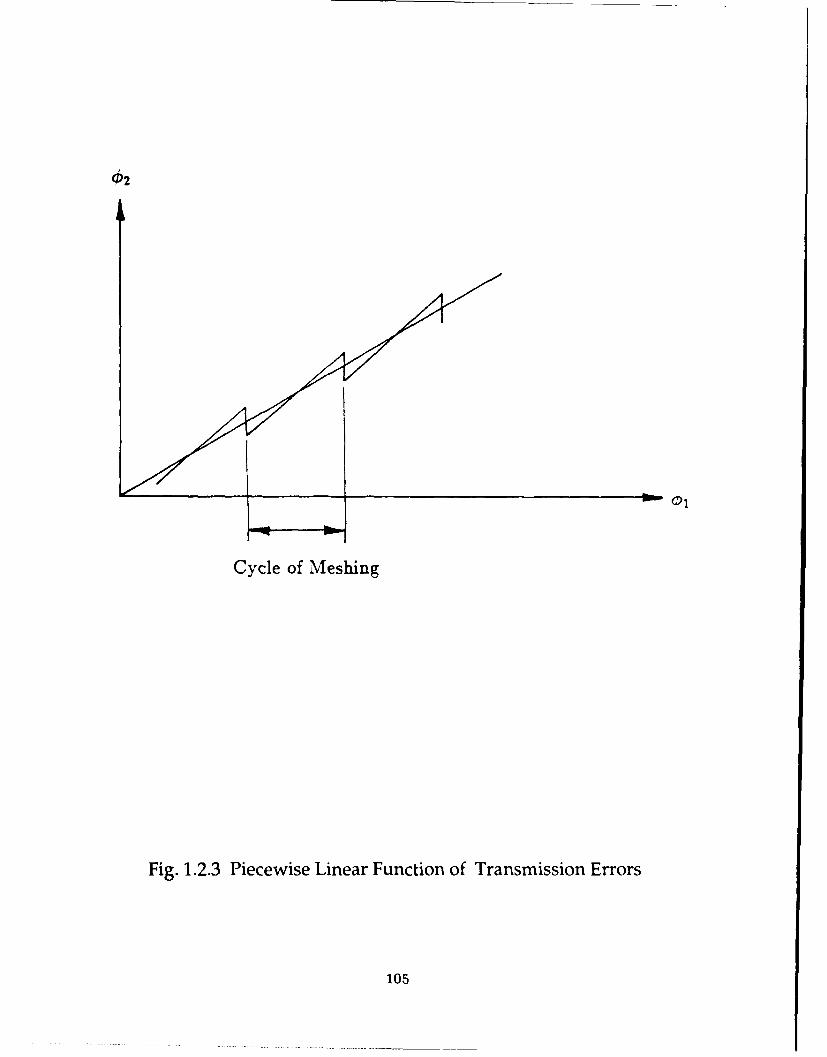
P2

Cycle of Meshing

Fig. 1.2.3 Piecewise Linear Function of Transmission Errors

105

(a)

(0)

(b) Cycle of Meshing02

(0))

01

Cycle of Meshing

Fig. 1.2.4 Parabolic Type of Transmission Errors

106

772

Fig. 1.2.5 Tangents of Contact Paths

107

4 eh

e.j

2b

Fig. 1.2.6 Orientation and Dimension of Contact Ellipse

108

Em,

Omi?

Od

i-Va VX2,

-vQa

(b) (c)

Fig. 2.1.1 Coordinate Systems and Pinion and Cradle Settings

109

Yd

0 M Xmi?4

E

Od Xd

Zd)

Fig. 2.1.2 Pinion Generation: Additional Coordinate Systems

110

nnn m mu oun wlm n nunnnnmammi ~ un nnumn ml~namOumnp

Xb

ObOe ,C

Fig. 2.1.3 Tilt of Pinion Head-Cutter

ill

(a) I.rn2 1c2

0m22

MT Xm2 Xc2

zc2--7n

(b)

c2 1 rrz2

I1p2

Op2

0m2

0c2 m

Fig. 2.2.1 Coordinate Systems and Gear and Cradle Settings112

(a) Yd2 m

XB2

0 d2

Zd2 Z,~2

(b)

-17d

Fig. 2.2.2 Gear Generation: Additional Coordinate Systems

113

\ h,

02R 72 r2

Fig. 2.3.1 Mean Contact Point

114

JlP

Fig. 2.3.2 Gear Generation: Instantaneous Axis of Rotation

115

HG

Yp,2

'rn2

y2)Op2 __ __ _ __ __ _

q20 m2 8'Xm2 t-Vc2

02

Zmn2

Fig. 2.3.3 Gear Head-Cutter Installments

116

z&p2

Fig. 3.1.1 Gear Head-Cutter

117

Pw

R.u2 -

Fig. 3.1.2 Point Diameter

118

Zdd

002

011

(a)

(b),

OF

(b))

c ZFZ

20

6-4F

o For Convex Side =(M

R m

OF R, p

Rep For Concave Side

C

OF Rrvp _f

ZF, Z,

Fig. 5.5.1 Pinion Head-Cutter Blades

121

Yn1

0M Xn ji(M)

444

Zd)O/~ 00r/X

122

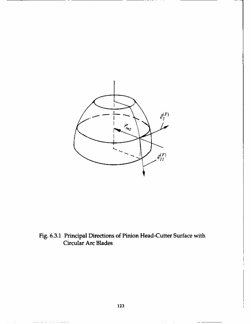
K e1

Fig. 6.3.1 Principal Directions of Pinion Head-Cutter Surface withCircular Arc Blades

123

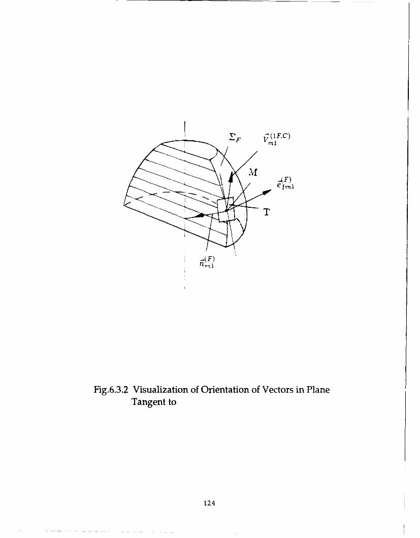
M F)

-.( F)

Fig.6.3.2 Visualization of Orientation of Vectors in PlaneTangent to

124

0O2

ILT

--

Fig. 6.4.1 Parabolic Function of Transmission Errors

125

i .,..... • X C

02 r2

Fig. 6.5.1 Coordinate Systems Used for Visualization of Contact Path

126

02 2

Z2

x2

Fig. 6.5.2 Mapping of Contact Point _N"

127

YC

Fig. 6.5.3 Coordinates of Points of Contact Ml and N"

128

J(ii

Fig. 6.5.4 Orientation of Contact Ellipse

129

Fi.7.. Loaino enCnatPito hfe ern otc

Pitch Con 13P

/ p

Face Cone GM

02 Root Cone /r

Fig. 7.1.1 Location of Mean Contact Point of Shifted Bearing Contact

130

x2

y h

2;2

Oh r

Fig. 7.1.2 Gear-Pinion 'Misalignment

131

CAM PROFILE AND ITS MOTIONb -5.5, E =15, TA3.6230

TCradle CenterOct

* Guide

Cam Rotation

q.q

o Cam

0

-20.0 -12.0 -4.0 4012.0 20.0

Fig. A.3.1 Cam Profiles and Guides

132

Yf

Ox0;

9q9

Fig. A.3.2 Schematic of Motions of Cam and Guides

without Modified Settings

133

(a)

CV

-

(b)

I2TL /

Fig. A.4.1 Coordinate Systems for Cam Mechanismwith Modified Settings

134

Yc

00:0

Cr

VvO p

Fi.A . rnmsio fCmRtto it rdeRtto

by~~~~, Modfe Stig

135

Transmission Error in Meshing Pe iGaear Ceaw~z Side - Mea

6

Use \ / / 0

A '41il

-2. 1. 1. 60 -. 00 40 80 1. 60 3.RotCmeGsrtrz(n

Fig. .1 CnatPtenad.asisinErr tGa en

Poiino2ovxSd

U) 13 I

Transmission Error in Meshing PeriodGear Couvez Side Too

V iN9 0.0

ag

X "'

(A i , 1

4 \ /292.GEA RTATONANGB dogoo

TOT ONAT.~rMGearCouvz S I

To /

-1. t. 80 -. .0 40 80 1. 60 2.RotCs eearz(n

Fi. .2Cotat ater ad rasmssonEror a GarTo PsiioofCnexSd

13

Transmission Error in Meshing PeriodGear Coavex Side - Heel

V u-8 ; H .3

! /

ix

-"A0 -L3.0 -4.0 4.0 13.9 20.0

G"AR ROTATION ANGLz (dogrow)

TOOTrH CONTAC'T PATTERBPNGear Convexr Side

e Heel V/H -0O / 3

A o

Root Come Gonoratrix (sam)

Fig. B.3 Contact Pattern and Transmission Errors at Gear Heel Positionof Convex Side

138

Transmission Error in Meshing PeriodGear Caca.s Side MEAN

V * 0; H - 0

0

Saz

0

La

2. 0- .9-.4.Me3.

GERRTTO0AGE(ere

MOHCNAC ATRGea Cocv i

MeniH82.

-20. 1. -1.S 0. -4.6 . .6 ' 12. 6 . 26.6

RoAt oTnsO GeeANGLE (mmr)

PoitonofCoGaea SideveSd

M..aV/139

Transmission Error in Meshing PeriodGear Concave Side - TOR

V -11: H 3

0)

U

o40401202.GIA OATO NLE(ere

TOT ONATPATRGerCnaeSd

To V/ 11

o

Z

14

Transmission Error in Meshing PeriodGear Cowrne Side - Heel

V m9: H -3

-2 . 20-. . 363.GERRTTO0AGE(ere

TOT ONATPATR

GerCsaeSd

14

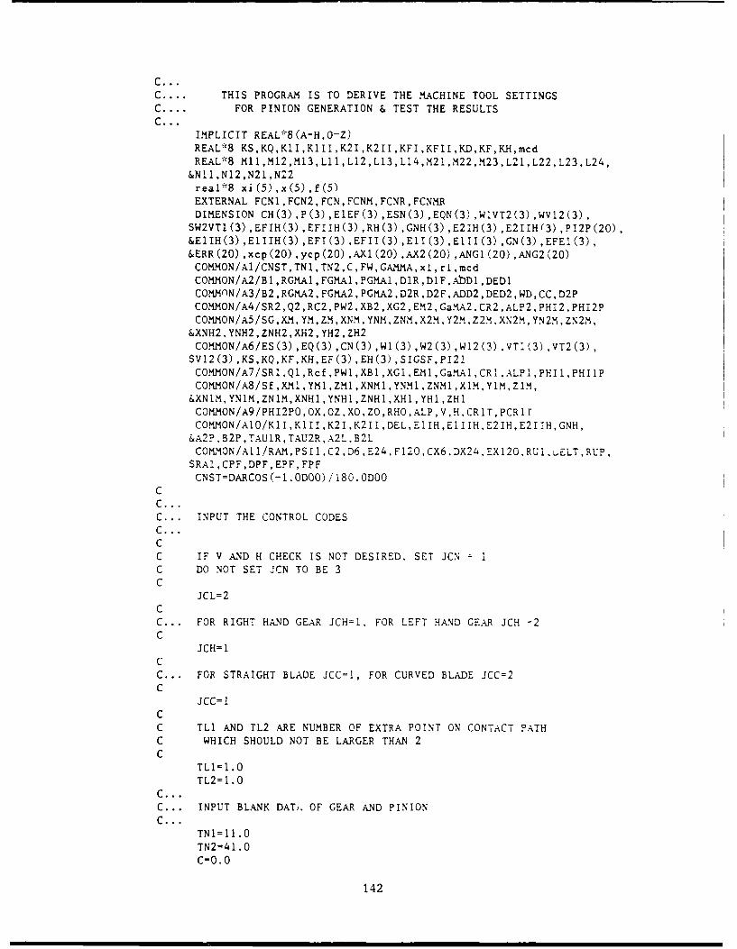
c ...

C .... THIS PROGRAM IS TO DERIVE THE MACHINE TOOL SETTINGSC .... FOR PINION GENERATION & TEST THE RESULTSC ...

IMPLICIT REAL'*8(A-H,O-Z)REAL*8 KS,KQ,K1I,KlII,K2I,K2II ,KFI,KFII,KD,KF,KH,mcdREAL*8 Mll,M12,M13,Lll , L2,L13, L14,M2l,m22,M23,Ll21,L22, L23, L24,

&N11 ,N12,N2l ,NZ2real *8 xi (5) ,x(5) ,f (5~)EXTERNAL FCNl ,FCN2, FCN, FCNM, FCNR, FCNMEDIMENSION CH(3),P(3),ElEF(3),ESN(3),EQN(3),W1VT2(3),WV12(3),

$W2VT1(3) ,EFIH(3) ,EFIIH(3) ,RH(3) ,GNH(3) ,E2IH(3) ,E2IIH(3) ,PI2P(20),&E1IH(3) ,ElIIH(3) ,EFI(3) ,EFII(3) ,E1I(3) ,E1II(3) ,GN(3) ,EFE1(3),&ERR(20) ,xcp(20) ,ycp(20) ,AX1 (20) ,AX2(20) ,ANG1 (20) ,ANG2(k20)COMMON/A1/CNST, TNl, TN2,C, FW, GAMMA, xi, r,mcdCOMMON/A2/Bl,RGMAI,FGMA1,PGMA1,DlR,D1F,AkbD1,DED1COMMfN/A3/B2,RGMA2,FGMA2,PGM-A2,D2R,D2F,ADD2,DED2,WD,CC,D2PCOMMON/A4/SR2,Q2 ,RC2, PW2. XB2 ,XG2, EM2 ,Ga.A2 ,CR2 ,ALP2, PHI2 ,PHI2PCOMMON/A5/SG,XM,YM,ZM,XNM,YNM,ZNM,X2M,Y2M4,Z2M,XN2m,YN2M,ZN2M,

&XNH2,YNH2,ZNH2,XH2, YH2,ZH2COMMON/A6/ES (3) ,EQ(3) ,CN(3) ,W1(3) ,W2(3) ,W12(3) ,VTI(3) ,VT2(3),

SV12 (3) ,KS,KQ,KF,KH, EF (3),EH (3),SIGSF, PI21COMMON/A7/SRI,Ql,Rcf,FWI,XB1,XG1,EM1,GaMiAl,CRI,AkLPI,PHI1,PHIlPCOMMON/A8/Sf,XMI,YMI,Z,1i,XNM1,YNM1,ZNM1,XlM,YlM,ZlM,&XN1M,YNiM,ZN1M,XNH1,YNHI,ZNH1,XH,YHI,ZH.COMMON/A9/PHI2PO,OXOZ,XO,ZO,RHO,ALP,V,H,CR1T,PCRifCOltMON/AIO/KlI, KlI,K2I, K2II, DEL, EIIHEIIIH. E2 IH, E2IIH, GNH,&A2P,B2P,TAU1R,TAUr2R,A2L,B2LCOMMON/A11/RAM,PSII,C2,D6,E24,Fl20,CX6,DX24,EX12O.RU1,uELT,RUP,

SRAI ,CPF,DPF,EPF, FPFCNST=DARCOS(-1.ODOO) /180.ODOO

C ...C ... INPUT THE CONTROL CODESC ...CC IF V AND H CHECK IS NOT DESIRED, SET JCN IC DO NOT SET JCN TOBE 3C

JCL=2CC ... FOR RIGHT HAND GEAR JCH=1. FOR LEFT HAND GEAR 3CR =2C

JCH=iCC ... FOR STRAIGHT BLADE JCC=1, FOR CURVED BLADE JCC=2C

JCCIlCC TLi AND TL2 ARE NUMBER OF EXTRA POINT ON CONTACT PATHC WHICH SHOULD NOT BE LARGER THAN 2C

TLi=1 .0TL2-1.0

C ...C ... INPUT BLANK DAT, OF GEAR AND PINIONC ...

TN1 11.0TN2='41.0C=0.0

142

FW27. 03GAMMA=90. 0*CNSTMCD76.56RGMAI= 13. 3333*CNSTBl=35.0*CNSTB2=35 .0*CNSTRGiIA2= 70. 6500*CNSTFGMA2= 76. 666 7*CNSTPGMA2= 74. 9833*CNSTD2R= 0.0D2F0.0ADD2= 2.06DED2=6.05WD= 8.11CC=0.81DEL0. O0025*25 .4

CC ... INPUT NORMINAL RADIUS OF GEAR CUTTER AND POINT WIDTH, BLADE ANGLEC

RU2=152.4000/2.0PW2= 2.79ALP2=20. 0*'CNSTDC22. 0*RU2

CC... INPUT THE SYNTHESIS CONDITION PARAMETERS AND PINION CUTTER BLADE

C ANGLE, ALP1(FOR GEAR CONVEX, ALP1>O, FOR GEAR CONCAVE ALP1<0)CC GEAR CONVEX SIDEC

F121--0.0008KD=0. 180ETAG=-65 .0OCNSTGAMA1= 13. 3333"CNSTRHO= 250.0C2= 0.00ALPl-18 .500*CNSTTNI-8.0

C ...SGN=DSIN (ALPi) /DABS (DSIN (ALPI))KSIDE=O

CC ...C

GOTO 1989

CC '~GEAR CONCAVE SIDEC1990 CONTINUE

F121= 0.0008KD=0. 180ETAG= 65.0'CNSTGAMA1=13. 3333*CNSTRHO- 200.0C2- 0.00ALF1=-21 .50*CNSTTNI-8.0

C ...SGN-DS IN(ALP 1)/DABS (DS IN (ALP 1))KSIDE-1jc1-2

143

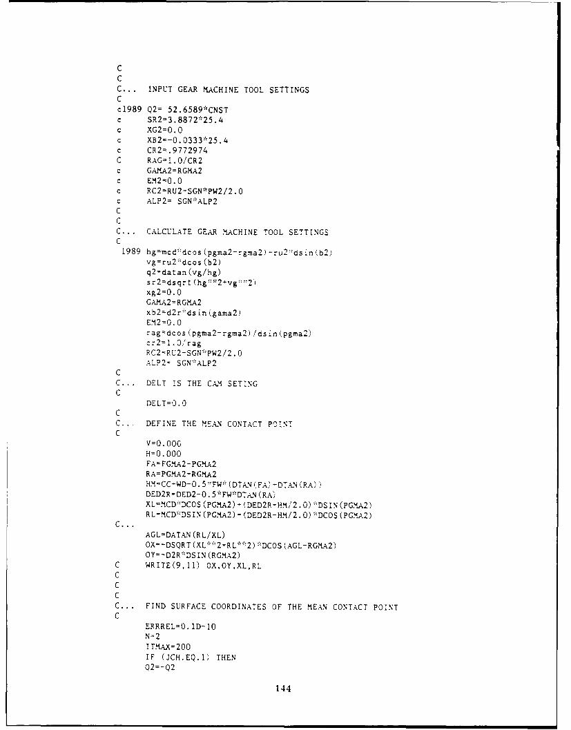
CCC ... INPUT GEAR MiACHINE TOOL SETTINGSCc1989 Q2= 52.6589*CNSTc SR2=3.8872*25.4c XG2=0O.Oc XB2--0.0333*25.4c CR2=.9772974C RAG-1.O/CR2c GAMA2=RGMA2c EM2=0.Oc RC2=-RU2-SGN*PW2/2.Oc ALP2= SGN'-"ALP2CCC ... CALCULATE GEAR MACHINE TOOL SETTINGSC1989 hgnmcd-dcos(pgma2-rgma2)-ru2"dsin~b2,

vgru2--.dcos (b2)q2=datani(vg/hg)sr2=dsqr-t(hg'2-vg 2)xg2=0.OGAMA2=RGMA2xb2=d2r'-dsin(gana2)E,12=0.O0rag~dcos (pgma2-rgna2) /dsin(pgma2)cr2=1.0/ragRC2=RU2-SGN""PW2/2. CALP2= SGN'*ALP2

CC... DELT IS THE CAM SETINGC

DELT=O.OCC... DEFINE THE MEAN CONTACT POINTC

V=O. 00H=0. 000FA=FGMA2-PGMA2RA=PGMA2-RGMA2H.M=CC-WD-O. 5-'FW' (DTA-Ni (FA) -DTA.N (RA))DED2R=DED2-O. 5'FW,'DT.AN (RA)XL=M'CD' DCOS (PGMA2) -(DED2R-HI/'2 .0) -'DS IN (PGMiA2 )RL=.MICD-,'DSIN (PGMA2) - (DED2R-HM/2.O0) -, DCOS (PGM.-A2)

C ...AGL-DATAN (RL/XL)OX=-DSQRT (XL'--2+-RL*"'2) *DCOS (AGL-RGIMA2)OY=-D2R'DS IN (RGMIA2)

C WRITE(9,1l) OX,OY,XL,RLCCCC .. . FIND SURFACE COORDINATES OF THE MEANL CONTACT POINTC

ERRREL=O. iD-10N= 2ITHAX=200IF (JCH.EQ.1) THEN02=-Q2

144

X1 (1) =270. 6*CNST+B2ELSEXI (1) =B2END I Fxi (2) -0. 0CALL DNEQNF(FCN1,ERRREL,N,ITMAX,XI,X,FN0RM)TH=X(1)PH=X (2)ST=DSIN (TH)CT=DCOS (TH)SH=DSIN (PH)CS=DCOS (PH)SP=DSIN (ALP2)CP=DCOS (ALP 2)SM=DSIN (GM.A2)CM=DCOS (GAMA2)THIG=TH

C WRITE(9,11) Xn2M,Yn2M,Zn2M,ZNM.YNM.ZNM)C WRITE(9,11) XM,YM,Z.M,sg,hnCC... DEFINE VECTORS TO COMIPUTER THE SECOND ORDER PROPERTY OF GEAR

CES (1) =-DSIN(TH-PH)ES (2) =DCOS (TH-PH)ES(3)> 0.0EQ (1) =SP*DCOS (rH-PH)EQ (2) =-SP--DSIN (TH-PH)EQ(3) =-CP

CN (1) =XNMCN (2) =YNMCN (3) =ZNMKS=CP/ (RC2-SG"SP)KQ=O. 0w1 (1) =-CMWl(2)= 0.0wi (3) =-smW2(1)= 0.0W2(2)= 0.0W2 (3) =-CR2VTI1 ()= Ym,"Sm+E42'SmVT1 (2) =-xm*sm+(ZM-XB2) '"C.MVT1 (3) =-YM*C.M-Em2 CmVT2 (1) = YM-"CR2VT2 (2) =-XM'*CR2VT2(3)= 0.0Do 10 1-1,3W12 (I)=W1 (I)-W2(I)

Vl12(I)=VT1 (I)-VT2(I)10 CONTINUE

C

C ... FIND THE PRINCIPAL DIRECTION AND CURVATURES AT MEAN POINT

CP121=0.0CALL CURVAI

C WRITE(9,12) KF,KH,SIGSF

C 12 FORMAT(3X,3(G14.7,2X))K21-KFK211-=KHPHI 2=PH/CR2sh2=ds in(phi2)

1 45

ch2-dcos (phi2)xX- CM*ef(l)+SM'cef(3)yY- ef(2)zZ--SM*ef (1) CM*ef (3)ef (1)=xxef(2)- CH2*yY-SH2*zZef (3) = SH2*yY+CH2*Z

C WRITE(9,11) xx,yy,zzC

xX= CM~eh()+SM*eh(3)yY= eh(2)zZ=-SM~eh (1) CM~eh (3)eh (1)-xxeh(2)= CH2'*yY-SH2'*zZeh(3)= SH2"yY+CH2**zZ

C WRITE(9,11) Ef(l),Ef(2),Ef(3)C WR ITE(9, 11) Eh(l),Eh(2) Eh(3)CCC

ERRREL=O. iD-10N1lIT.MAX=200XI (1)=O.OCALL DNEQNF(FCN2,ERRREL,N,ITMAtX.XI,X.FNORM)PHI2PO=X (1)

C WRITL(9,11) X(1)C WRITE(9,11) XH2,YH2.ZH2C WRITE(9,11) XNH2,YNH2,ZNH2C

CHP=DCOS (X(i))SHP=DS IN (X(1) )C MM =DCO0S (GA~I)SMM=DSIN (GAM hA)XX= ef(l)YY=-ef (2) '--CHP+ef (3) .shpZZ--ef (2) *SHP-ef (3) "chpEF(l)= XcC.i+zz',SlmNef(2)- YYEF (3) -- XX SMZZ--CM.i

C ...

XX= eh(i)YYeh (2) *CHP-eh (3) -shpZZ--eh (2) *SHP-eh (3) *chpEH(l)- XX*CM+~,ZZ*SMM4eh(2)- YYEH (3) -- XX*SMMi.ZZ*CimN

C WRITE(9,11) -F(l),EF(2),EF(3)C WRITE(9,11) EH(l),EH(2).EH(3)

ETAG=90. O*CNST+S IGSF+ETAGCC LOCAL SYNTHESIS AT MEAN CONTACT POINTCC...

RH (1)-XH2RH(2)-YH2RH (3) =ZH2GNH (1)-XNH2GNH (2)-YNH2G;NH (3)-ZNH2

146

E21H(1)= EF(i)E21H(2)= EF(2)E2IH(3)= EF(3)E21IH(1)= EH(l)E211H(2)= EH(2)E2IIH(3)= EH(3)K2I=KFK21I=KH-

C ...C... RELATIVE MOTION PARAMETERS IN GEAR & PINION MESHING PROCESSC...

R12=TN1/1N2Wi (1)=-1 .0000Wi1 (2) =0. ODOOWi (3) =0. ODOOW2 (1) = R12'~MW2(2)=0.ODOOW2 (3) =-R 12 "SMIMW 12 (1)-Wi1 (1) -W2 (1)W 12 (2) =Wl (2) -W2 (2)W 12 (3)-Wi1 (3) -W2 (3)VT1(i)- 0.0000VTi(2)= ZH2VTI (3) =-YH2VT2(i)= Ri21"(YH2-C)--'SMMVT2(2)-R2(XH2-SM-ZH2',CMM4)VT2(3)- Ri27(YH2-C)"CMMV!2(1)= VT1(i)-VT2(i)V12 (2) = VTI (2) -VT2 (2)V12(3)= VT1(3'J-VT2(3)

C WRITE(9,3) Vi2(i),VI2(2),Vi2(3)C3 FORMAT(5X,3G!4.7,/)C ...C ... CALCULATE THE COEFFICIENT A13.A23,A33

ESN(i)= GN'H(2):.E21H(3)-GiNH(3W:IE2IH(2I

ESN(3)= GNH(i>*E2IH(2)-GNH(2) 'E2IH(,')C ...

EQN(1)= GNH(2) '.E2IIH(3)-GNH(3)'.E2IIH(2)

EQN (3) = GNH (1) -E2 IH (2) -GNH (2) :E2iIH (1)C ...

WIVT2(i)= W1(2')".VT2(3-Wi(3)*VT2(2)

W2VT(i)= W2(2)*~VTI(3)-W2(3)*cVTi(2)W2VT1 (2) =- (W2(1)*'VT1 (3) -W2 (3)*VTi (1))

C ...V 12S=0. 0D0Vi2Q=O.ODOWNES=O. ODODWNEQ=O.ODOOVWN= 0.0000

147

W1TN=O. 0000W2TN-O.ODOOVT2N=0. ODOO

C ...DO 1 1-1,3

V12S= V12 (I) *E2IIH(I)+vl2

WNES= W12(I)*ESN(I)-WNESWNEQ= W12(I)'*EQN (I)-.-WNEOVWN -GNH(I)*wv12(I)+VWNW1TN=GNH(I) *W1VT2(I)4+W1TNW2TN=GNH(I)*~w2VT1 (I)+W2TNVT2N= GNH (I)*~VT2 (I) +VT2N

I CONTINUEC WRITE(9,6) V12S,v12QC 6 FORMAT (5X,2G14.7,/)C ...C ... COMPUTER THE COEFFICIENTS A13,A23,A33C...

B13=-K21*Vl2S-WNESB23=-K2I*Vl2Q-WNEQ

C ...C... LOCAL SYNTHESIS OF MESHING AT MEAN CONTACT POINTC ...

DL=KD'FWSIGK2= K21+K2IISIGG2= K2I-K2 ITA=DEL/DL*"2Tl=-B13-"vl2Q+ (B33-Bl3"'-V'.2S) 'DTA.N ETAG)T2=B33+B23*IV12Q-V12S',-DTAN(ETAG),ETAP=DATAN (TI/T2)VSI mB33/ (Bl3-B23'-DTAN (c-EAP'))AMl=DSIN(ETAP)*"2AM2=-DSIN(2.ODOO*ETAP) /2.0000AN I=(B13-B23*DTN(ETA?"/(1. D04-DAN(E-,AP),, .2)'IS IAN2=(B13'*DTAN(ETAP)-B23)/((1.ODOO+DTA-%.N(E'AP) '"2"!vSl)SGN=DSIN(ALP1) /DABS (DSIN(ALPI))A=A'*SGNSIK (.DOA 2 (,N "-2A2""1)/ 2.ODOO A-(A-1iv.DCUS2.ODOO-,.

&ETAP) +AN2*DS IN (2. ODOO"*ETAP )))SIGKI= SIGK2-SIGKT1= 2.ODOO0-N2-SIGKDSIN(2.ODOO*ETAP)T2=SIGG2-2.ODO0*ANl-SIGK*DCOS (2.ODO0"'ETAP)SIG12=.50D00;'DATA4N(Tl/T2)SIGGI=(2.OD00*AN2-SIGK'DSIN(2.ODOO-ETAP))/DSIN(2.0DOO SIG12)KI = (SIGK1+SIGG1) /2.0000KIII1=(SIGKI-SIGG1) /2. 0000

C..C..C..C WRITE(9.11) ETAP.K1I.K1IIC WRITE (9,11) SIGK,SIG12,SIGK1 ,SIGGIC WRITE(9,8) T1,T2C 8 F0RMAT(5X,3G14.7)C..C..C...

C... PRINCIPLE DIRECTIONS OF PINION SURFACE AT POINT MC ...

148

DO 15 I=1,3

15 CONTINUEC WRITE(9,11) E1IH(1),E1IH(2),E1IH(3)C WRITE(9,11) ElIIH(l),E1IIH(2),ElIIH(3)C ...C .. . COINCIDE THE NORMALS OF CUTTER AND THE PINION SURFACESC ...

SM1=DSIN (GAMAl)CM1=DCOS (GAMAl)SP-DS IN (ALP 1)CP=DCOS (ALP 1)Tl=- (XNH2-'SP""SM1)T2= CP*CM1

IF (JCH.Eo.1) THENTHF=DARCOS (T1/T2)ELSETHF=DARCOS (T1/T2)THF=360. O*CNST-THFEND IFBAI=-CP-"DSIN (THF)BA2= CP'"DSIN (GAMAI) '--DCOS (THF) -SP"'DCOS (GAMAI)TT=-(YNH2**2,ZNH21'12)CSH=- (BA1',"YNH21-BA2-'ZNH2) /TTSNH= (BA2'*YNH2-BA1'-"ZNH2) 'TTPHIH=2.0*DATAN2(SNH. (1.ODOO--CSH')

C WRITE(9,8) THF,PHI-CC... FIND THE PRINCIPALT DIRECTIONS OF PITNION GENERATING SURFACEC

EFI (1)=-DSIN (THE)EEI(2)= DCOS(THF)E-lI(3)= O.ODOOEFII (1)= SP*DCOS(THF)EFTII(2)= SP*DSIN(THF)EFII (3)=-CP

C WRITE(9,11) EFI(1),EFI(2),EEI(3)C WRITE(9,jl) EFII(1),EFII(2),EFII(3)CC ... FIND THE PINION PRINCIPAL DIRECTIONS IN SYSTEM S41C

XX= E1IH(1YY= DCOS(PHIH)"E1IH(2ytDSIN(?HIH)-,1.IH(3)ZZ=-DSIN (PHIH) "eE1IH (2) -DCOS (PHIH) "'E1IH (3)

E1I(2)= YYE1I(3)= SN1*XX+CMI*ZZ

CXX= E1IIH(1YY= DCOS(PHIH)*ElIIH(2)-DSIN(PHIH).?EIIIH(3)ZZ=-DSIN (PHIH) *EIIIH (2) DCVS (PIII) "'IIH (3)EIII(1)= CM1*XX-SM1I*ZZE1II(2)= YYE1II(3)= SM1'*XXICM*ZZ

CC ... FIND THE UNIT NORMiAL IN SYSTEM SMIC

XX- XNH2YY- DCOS(PHIH)"YNH2,DSIN(PHIH)""ZNH2

14q

ZZ=-DSIN (PHIH) *YNH2+DCOS (PHIH) *ZNH2GN(1)- CM1*XX-SM1*zzGN(2)- YYGN (3) = SMI*'XX+-CM1 ZZ

CC ... EXPRESS THE POSITION VECTOR IN SMIC

XX= XH2YY= DCOS (PHIH) *YH2+DSIN (PHIH) ,,ZH2ZZ=-DSIN (PHIH)*~YH2-DCOS (PHIH) "ZH2RX= CM1*XX-SM1*ZZRY- YYRZ= SMI*XX+CM1*'ZZ

C XX=-CF*DCOS(THF)C YY=-CF'-DSIN(THF)C ZZ=-SPC ...C WRITE(9, 11) ElI (1).EII;(2) .ElI (3)C WRITE(9,11) ElII(1},EI>: 2.ElII'3lC WRITE(9,1l) GN(1),GN(2),GN(3)C WRITE(9,11) XX,YY,ZZC WRITE(9,11) RX,RY.RZC ...

DO 20 I=1,3XX=-EFI (I)EFI(I)= EFII(I)EFII (I)=XX

20 CONTINUECC WRITE(9,ll) ElI(l),E11k2),Ei!I(3)C WRITE(9, 11) EiII(l. .El::(2) .::I 'JC ...C... FIND THE ANGLE FORMED BETWEEN PR:-NCIPAL CURVA;TURESC ...

EFEl (3) = EFI (1) 'E1 (2) -E-l (2) " E1: (: )T1=O.ODOOT2=0.ODOODO 30 I=1,3

30 CONTINUESIGFI=2.0 O-DATA N2 (Ti,1. O-T2)

CC ... FIND THE CURVATURE OF PINION GENERATION SURFACE AT MEAN POINTC

IF (JCC.EQ.1) THENKFI=O.O

Bll=KFI-KlI'-DCOS(SIGF1) --2-KlII*"DSIN(SIGF1) ',-"2TKK= KI*SNSG I-"*- lI-C SSG I""'KFII=(B12*~*2#Bll' TKK)/Bl

C WRITE(9,11) SIGFI,KFIICC... FIND THE CUTTER POINT RADIUS AND ITS CENTERCC SF=SG*"DCOS (ALP2) /DCOS (ALPI)

SF=DABS (RZ) /DCOS (ALP 1)RCF=CP/DABS (KFI I) -SF-"SP

1 50

DO 40 1-1,3

40 CONTINUERCX- RX-SF*EFI(1)+RCF*P(1)RCY- RY-SF*EFI (2) +RCF*P (2)RCZ- RZ-SF*EFI (3) -RCF*P (3)

C WRITE(9,11) RCF,SFC WRITE(9,11) RCX,RCY,RCZ

ELSEKFI=1 .0/RHOB12=0.5DOO*(KI-KII)*~DSIN(-2.ODOO*SIGF1)

TKK= Kl*SNSG1*2KI*CSSG1;"KFII-(Bl2*~*2+Bl1*TKK) /Bll

C WRITE(9,11) SIGF1,KFIIDBT=-RZRM=CP/DABS (KFII)zo=- (IBT+RHO*SP)XO=RM-RHO*CPRCF=XO+RHO*DSQRT(1 .0- (ZO/RHO) " '2)RCX=RHO*GN (1)-XO"'DCOS (THE) -RXRCY=RHO'*GN (2) -XO*DSIN (THF) -RYRCZ=RHO*GN (3) -Z04RZ

C WRITE(9,777) XO,ZOC777 FORMAT(3X,' XO, XO =',2(2X,G14.7))C WRITE(9,11) RCF,RM,DBTC WRITE(9,11) RCX.RCY,RCZ

END IFCCC ... THE FOLLOWING IS TO FIND THE CUTTING RATIOC

CSM 1 CM 1SNM1=SM1TlX-EFI(1)TlY=EFI (2)

T2X-EFII (1)T2Y=EFII (2)T2Z=EFII (3)XN=GN(l)YN=GN (2)ZN=GN (3)RXC=RXRYC=RYRZC=RZ

CC WRITE(9,11) RCX,RCY,RCZC WRITE(9,11) TLX,TIY,TlZC WRITE(9,11) T2X,T2Y,T2ZC WRITE(9,11) XN,YN,ZNC WRITE(9,11) RXC,RYC,RZCC ...C ... THE FOLLOWING IS TO DETERMINE DELTA,.M1,AND IFM

C ...Mll1,XN*TY-YN*T1XM12=--CSMI* (YN'*Tlz-ZN*-TIY)M2 1 XN*T2Y- YN"*T2XM22--CSMI'*(YN*T2Z-ZN*T2Y)

C WRITE(9,11) Ml1,M12,M421,M22

C L11=(B12/B11*M11I-M21)/KFIIC L12-(B12/Bl11*M12-M22)/KFIIC ...C L21=-T2Z/TlZ*LllC L22=-T2Z/TIZ*Ll2-RYC-"'CSM1/T1Z

DTT=Bl2*KFI*T2Z4B1 VKFII*TIZ

Ll=T /DTTM2-I2"ll/T

L21=T2Z*(B11".M21-Bl2*.M11)/DTT

C WRITE(9,11) L11,L12,L21,L22Xl 1=L21'*TlX+-L1 1T2XX12=L22*T1X+Ll2*T2XX21=L21*TlY+L1 1*T2YX22=L22*T1Yi-Ll2"T2YX31=L21"-'TIZ±LI 1*T2ZX32=L22*TlZ+Ll2*T2ZEl1=YN*X11-XN*X21E12=YN"-X I 2-XN"-X22-ZN---X2 1 "CSM I- YN"X3 1 '"CSM IE13=- (ZNX22-YN*X32) <CS.11Y1 1=-XN*~(RXC'*SNMI-RzC-'*CSM1 -YN-"RYC"SNM1iY12=Y1 1SNM1X13=Xl2-RYC'*SNM1X23=X22+RXC"'SNM1-RZC'-'CS.1X33=x32+RYC*CSM1

Y22=-XN--X23--SNM1+YN,- (SNM -"X13-CSMPl- X33) -ZN'-'X23..CS-MICC ...CC ...C ... THE EFFECT OF SECOND ORDER RATIO OF ROLL ON A33

Th1=XN'"XI -YN'X21-ZN'X3i,

C WRITE(9,163) TMI,TM2C163 FORNAT(2X,'TM1,TM12 ',2(2XG14.7))

ZZ1=C2*TM1lZZ2=C2* TM2-SNMP, TIM IZZ3=C2!"SNM1*TM2

C ...C Z1=KFII',L11 -2-EllC Z2=2.ODOOKFII-"L11""Li2-E-12-Y2V-YlC Z3=KFIIVLI2*.2-E3-Y2-Y2

Z3=KFI*L22,'24KFII*L12"'---2-13-Y22.-Y12+ZZ3NIl=KFII*L11+M21N12=KFI I*Ll2+M22N21=KFIV L21±M11N22 =KF I -L2 2*M 2

C WRITE(9,11) B!2,Z1,M11,Ni1AA=B12'*Zl-N21*1 1BB=Bl2'Z2-N21*Nl2-N22Th1 1CCC=B12''Z3-N22*NI2

r WRITE (9,11) AA,BB,CCCIF (AA.GT.O.OOODO1) GOTO 1949T1=-CCC/BBGOTO 1950

1949 T1=(-BB+DSQRT(BB,"2-4.0D0O7'AACCC)/(2.01DOO'-.AA%1950 FM1=T1+SNM1l

152

CR1=FM1RAP=1. 0/CRIVF3=X31*~Tl+X32+RYC*CSMI

C ...

C...C ...C ... THE DETERMINATION OF EM AND DELTAC ...

EM1= (Xl 1'T1 RYC""FM1-X13) /FM1XG1= (X21*Tl-RXC-'FM11-X23) /(FM1*CSM1I)

C ...RCX=RCX-XG1*CSM1RCY=RCY-EM1RCZ=RCZ-XGI','SNM1

C ...Vl=RCYHl=RCXXBl=RCZSR1=DSQRT(V1".2-Hl1'-*2)'Q1=-DARSIN (V1/SR1)XB1=-XB1

CC .... DETERMINE THE CAM SETTINGC

RA11 . 0/CRIRAM=TN1/TNlI".RAlPSII= DATAN (C2-"RAM/ (RAM-l. 0)RUP=15.0*DCOS( PS 'i')/ ,RA.9->.O)RU1=RUP

C DELT=O.0C

CALL CAMC WRITE(9,191) RU?C WRITE(9,191) RUlC191 FORMAT(2X,'RU1 DELT = ',2(2X,G14.7)C WRITE(9,199) RAI,C2,D6,E24,F120C WRITE(9,199) RA1,CF,DPF,EPFFPFC 199 FORMAT(2X,'CA ,',2X,5(2X,G14.7))CC ...CC WRITE(9,25) F.41C 25 FORMAT(5X,' F.41 = ',G14. 7)C WRITE(9,44) EH1,SR1,Q1C44 FORMAT(2XJ'EMI,SRI,Ql',3(3X,G14.7))C WRITE(9,45) XG1,XBI,V1,H1C45 FORMAT(2X,'XGI,XB1,V1,H1',4(2X,G14.7I))C...

IF (KSIDL.EQ.O.O) THENWRITE (9. 131)

131 FORMAT(/2X,$ 2X, '" OUTPUT FOR GEAR CONVEX SIDE ~

& 2X ~ ........................................ ......... IELSEWRITE (9 ,331)

331 F OR MAT (/ 2X, '***** ,c*'* '**--** ,,*"****.-1.**,',**-' .-, 1* ;-,-. I-I /r 2X, '" OUTPUT FOR GEAR CONCAVE SIDE

& 2 x( , ...........

END IFWRITE (9, 13)

153

13 FORMATU (2X,'/$ 2X, "' GEAR CUTTER SPICIFICATIONS

& 2X , ~,r ,,**********

WRITE(9,115) DC2,PW2,ALP2

115 FORMAT(/2X,' GEAR CUTTER DIAMETER DC2 ,G14.7,/

$ 2X,' CUTTER POINT WIDTH : PW ' ,G14.7,/& 2X,' CUTTER BLADE ANGLE : PHI2 ,G14.7,//)

WRITE(9,3)

3 FORMAT (/2X, '$ 2X,'* BASIC GEAR MACHINE-TOOL SETTINGS ' ' ,/

& 2X, '***,:,r * ************************* *-,WRITE(9,4) Q2,SR2,XG2,XB2,EM2,GAIA2,RAG

4 FORMAT(/2X,' BASIC CRADLE ANGLE : Q2 ' ,Gl4.7,/& 2X,' RADIAL SETTING : SR2 ,Gl4.7,/

# 2X,' MACHINE CENTER TO BACK : XG2 ,Gl4.7,/

# 2X, SLIDING BASE XB2 ,G14.7,/$ 2X, BLANK OFFSET EM2 =' ,Gl4.7,/

# 2X,' .ACHINE ROOT ANGLE GAiA2 = G14.7,/

# 2X, RATIO OF ROLL RAG ,G14.7,//)WRITE(9,6)

6 FORMAT(//2X, ' ...............& 2X.'" BASIC PINION MACHINE-TOOL SETTINGS ,

WRITE(9,7) ALPI, RCF, QI,SRI,XGI,XBI,EMI,GAMAI,RAP

7 FORMAT(/2X,' BLADE ANGLE : ALP! = ,G14.7,/

& 2X, POINT RADIUS RCF ,G14.7,/& 2X,' BASIC CRADLE ANGLE Ql ,G14.7,/$ 2X, RADIAL SETTING : SRI

& 2X, .MACHINE CENTER TO BACK : XGI .014.7./S 2X, SLIDING BASE : XB- .G14.7,/

& 2X, BLANK OFFSET : EM! ,G14.7,/$ 2X, ,iACHINE ROOT A-NGLE : GALAt ,G14.7,,/& 2X,' RATIO OF ROLL RAP ,G-., i.IF (JCC.EQ.2) THENWRITE (9,61)

61 FORAT (//2X. ' .... .....

& 2X,'77 COORDINATES OF THE CENTER C _HE ARC t7','

WRITE(9,71) XO,ZO

71 FORMAT(/2X, ' RADIAL COORDINATE XO ' 014.7,.& 2X,' AXIAL COORDINATE ZO =

' ,G14.7,//)

ELSE

GOTO 1919END IF

1919 C)NTINUEWRITE (9,16)

16 FORMAT (//2X,.. . ....................... ........-..

& 2X,''CAM SETTINGS AND COEFFICIENTS OF TAYLOR SERIES . ,/

& 2X,.................-"-...-.-.,,...-.-..-.-- . -....-............-7

WRITE(9,17) PSI1, RUP, DELT, RA1,C2,D6,E24, F2"17 FORMAT(/2X, GUIDE ANGLE : PSI = , 4.,

& 2X, CAM PITCH RADIUS PUP ,G'4.7,& 2X,' CAM SETTING : DELT = .7,& 2X,' 1ST ORDER COEFFICIENT RA .

& 2X,' 2ND ORDER COEFFICIENT C2 '01.7,

& 2X,' 3RD ORDER COEFFICIENT: D6 0.7,& 2X, 4TH ORDER COEFFICIENT : E24 = G4..7

& 2X,' 5TH ORDER COEFFICIENT F,2Q , ..

C

C... CALL TCA

154

CC ..C ... DEFINE THE INITIAL POINTC ...C ...

XI (1)THIGXI(2)= 0.000000XI (3)-THFXI (4) =0.0XI(5)= 0.00

CC... FIND THE INITIAL CONTACT POINTC5555 N=5

ERRREL=0. iD-10ITMAX =200PH12P=PHI2POIF (JCC.EQ.1) THENCALL DNEQNF(FCN,ERRRELN,ITN'AX,XIX,FNORM,ELSECALL DNEQNF(FCNR,ERRRELN,ITMAX,XI,X,FNORM)END IFPHIIPO=X(5)

CCCC

PH 'P =H 2 O 10 0*N 7',N -T ,L-8 . C T''6 o N2PHI2P2=PHI2P0+180.0'CNST/TN2-TL2""180.0' CNET/ (6.0-"TN2)

PH12P=PHI2Pl333 CONTINUE

IF (JCC.EQ.1) THENCALL DNEONF(FCN,ERRREL.NITMAX.XI,X,FNORM)ELSECALL DNEQNF(FCNR,ERRREL,NITMiAX.XI,X.FNORM'END IF

C XI(l)=X(1)C XI(2)=X(2)C XI(3)=X(3)C XI(4)=X(4)C XI(5)=X(5)CC ... find the transmission errorCC ERRR=PH12P-PHI2P0-TNI/TN2*(X(5)-PHIlP0)

LkRPH12P-PHI2PO+TN1/TN2*(X (5) -PHIlPO)ERR (KK) =3600. 0*ERRR/CNSTP12P (KK) =PH12P

CC... computer the contact pathC

xlc= x2mrlc- dsqrt (y2m*~*2+z2m**2)xcp(KK)- xlc*dcos(rgma2)+rlc~dsin(rgma2)+oxycp(KK)--xlc*dsin(rgma2)4rlc*dcos (rgma2)+oy

CC... COMPUTER THE PRINCIPAL DIRECTIONS AND CURVATURES OF GEARC

TH-X(l)

155

PH-X(2)ST-DSIN (TH)CT-DCOS (TH)SH-DS IN(PH)CS-DCOS (PH)SP-DSIN(ALP2)CP-DCOS (ALP2)SM-DSIN (G.AMA2)CM-DCOS (GAMA2)

CC... DEFINE VECTORS TO COMPUTER THE SECOND ORDER PROPERTY OF GEARC

ES (1)=-DSIN (TH-PH)ES (2) = DCOS (TH-PH)ES(3)= 0.0EQ(1) =-SP*DCOS (TH-'PH)EQ (2) =-SP*DS IN (TH-PH)EQ (3)=CCN (1)=XNMCN (2)=YNMCN (3)=ZNNKS-'CP/ (RC2-SG*SP)KQ0. 0Wi (1)=-CMWl(2)= 0.0wi (3) =-SNW2(1)= 0.0W2(2)= 0.0W2 (3) =-CR2/T1(iI)= Y,%SN--EM2""SN

VT1 (2)=-XM*SM-(ZX',-XB2)'CM4VT1 (3)=-YM"C.-EM42*QVT2(1>'= YM*CR2VT2 (2) =-XM'*CR2VT2(3)= 0.0DO 110 1=1,3W 12 (1)=W 1 (1) -W2(I)V 12 (1)=VT 1 (1) -VT2 (I)

:10 CONTINUECC

P121=0.0

CALL CURVAlK21=KFK21 I=KHPH12-PH/CR2sh2=dsin (ph i2)ch2=dcos (rhi2)xX- CM~ek'(1)+SM~ef(3)YY ef(2)

zZ='-SM'~ef (1) CM'ef (3)ef(l1=xxef(2)= CH2*cyY-~SH2*czZef (3) = SH2'*yY+CH2'*zZ

c

xX-' CM~eh(l)+SM~'eh(3)yY- eh(2)zZ-S~eh()CM~eh(3)eh(I) xxeh (2)= CH2*yY-SH2*czZ

156

eh (3) = SH2*yY+CH2*ZC ...

CHP=DCOS (PHI2P)SHP=DSIN (PHI2P)CMII=DCOS (GA.MMA)SMM=DS IN (GAMM.A)XX= ef(1)YY-ef (2) *CHP+ef (3) *shpZZ=-ef (2)*'SHP-ef (3) *chpE21H(1)= XX*CMM+ZZ*SMME2IH(2)= YYE21H (3) =-XX*Smli~tZZ*Cm?1

C ...XX= eh(l)YY-eh (2) *CHP+eh (3) *'sj.pZZ=-eh (2) *SHP-eh (3) *chpE211H(1)= XX*ICMM+ZZ*SMME2IIH(2)= YYE21IH (3) =-XX"'SHM+ZZ',CMM1

CC ... COMPUTER THE PRINCIPAL DIRECTIONS AND CURVATURES OF PINIONC

TH1=X(3)PHI=X(4)STP=DSIN (TH1+PHl)CTP=DCOS (TH1-sPHI)IF(JCC.EQ.1) THENSP1=DSIN(ALPl)CP1=DCOS (ALP 1)ELSESGN=ALP1/DABS (ALPI)ALP=SGN*ALPSP1I=DS IN (ALP)CP1=DCOS (ALP)END IFSM-DS IN (G.AMAl)CM1=DCOS (GAMAl)

CC ... DEFINE VECTORS TO COMPUTER THE SECOND ORDER PROPERTY OF PINIONC

ES (1)=-STPES(2)= CTPES(3)= 0.0EQ(1)= SP1'*CTPEQ(2)= SP1*STPEO(3)=-CP1CN(1)=XNM1CN (2)=YNM1CN (3)=ZNM1IF (JCC.EQ.1) THENKS=CP1/ (RCFs+SF*SPI)KQO0.OELSEKS=DCOS (ALP) /(RHO*~DCOS (ALP) .XO)KQ=1 .0/RHOEND IFwl(1)= CM1w1(2)= 0.0W1(3)= SMiW2(1)= 0.0

157

W2 (2) - 0. 0W2(3)- CRiTVT1 (1) -Ym1*Sml-Em1*SMIVT1 (2)- XM1*SM1- (zM1-XB1) *CMIVT1 (3)- YM1*CM14EM1*CM1VT2 (1)--YM1*CR1TVT2(2)- XM1*CRlTVT2(3)= 0.0Do 210 1-1,3W12 (1)-Wi (I) -W2 (I)V 12(1) -VTl (I) -VT2 (I)

210 CONTINUECC

P121-PCRlT

CALL CURVAIC WRITE(9,12) KF,KII,SIGSF

Ki I=KF

C PHIl=PH1/CR1SH1=DSIN(PHI1)CH1I'DCOS (PHI 1)XX- CM1*EF(1)+SM1*EF(3)yYY ef(2)ZZ=-SM1*EF (1) +CM1*EF (3)ef (1)=EF(2)= CH1*YY+SH1'*ZZEF (3) =-SHl*YY-rCHI"-ZZ

XX= C~f1*EH(l)+SM1.El(3)yY= eh(2)

eh (1>xxEH(2)= CH1I*YY+SHI*ZZEH (3) =-SH1IrYY+CHl*ZZ

C ...CH1P=DCOS (X (5))SHIP=DSIN (X (5))ElIH(l)=EF(1)El IH(2) = CH1P'*EF (2) -SHlP*EF(3)ElIH(3)= SHIP*EF(2)+CH1P*EF(3)ElIIH(l)-EH(l)ElIIH(2)= CHlP*EH(2)-SHlP*EH(3)E1IIH(3)= SH1P*EH(2)-CH1P*,"EH(3)DO 109 1-1,3ElIH(I)=-ElIH(I)ElIIHN(I) =-EIIIH (I)

109 CONTINUECC ... COMPUTER THE DIMENSION AND ORIENTATION OF THE CONTACT ELLIPSE

CGNH (1)=XNH2GNH(2)=YNH2GNH (3)=ZNH2CALL ELLIPAX 1 (K) = A2 LAX2(KK)=B2LANGi (KK) =TAU1RANG2 (KK)-'TAU2R

C

1 58

KiKi(K+ 1PH12P-PHI2P+ 180.0*CCNST/ (TN2*'6.0)IF(PHI2P.LE. (PHI2P2+O.O0') GOTO 333

C..C..

WRITE(9, 441)441 FORMAT (I

& I TRANSMISSION ERROR IN A MESHING PERIOD$ /- r -ft*****$. .. . . . . ... .1

CDO 444 I=1,KK-1PI2P(I)=PI2P(I) /CNSTWRITE(9,555) P12P(l),ERR(l)

555 FORMAT(3X,3(GI4.7,3X))444 CONTINUEC

WRITE (9, 551)551 FORMAT(/,

& /, CONTACT PATH FOR A PAIR OF TEETH IN MESH

DO 666 11I,KK-1WRITE(9,747) XCP(I),YCP(I)

747 FORMAT(3X,2(G14.7,3X)<'666 CONTINUE

CWRITE(9,661)

661 FORMAT/,'~..........................& ,'~DIMENSION A.ND ORPJENTAT :CN OFCOTC ELPS

DO 888 I=i,KK-1wRITE(9,889) .kXING AX2(:) A.SG2(:)

889 FORM.AT(3X,4(G14.7,3X))888 CONTINUE

CCC

IF(JTCL.EQ.1) GOTO 1111IF-(JCL.EQ-.3) GOTO 11.3

CC ... V AND H CHECK FOR TOE POSITIONC

HMT=WD-CC-3 .0,/4. O':FW" (DTAN FA) -DTA-N(RA-)DED2T=DED2-3.O/4.0-O'W'DT.A.N (RA)T.MCD=.4CD-O. 25:-FWXL=TMCD -DCOS (PGM'A2) - DED02T-HUT/2. 0 DS IN, ?cMiA2)RL=TMCDfDS IN (?G.NA2) - (DED27,-HMT/2. 0) ' -DCOS (PGM-A2)

CC ... FIND THE MEAN CONTACT POINT ON THE GEAR SURFACEC

ERRREL=0. 1D-7N=2ITAxW=200IF (JCH.Eo.1) THENXI (1)=270.0'CNST-B2ELSEXI (1)=B2

C XI (1) =90. 0;-CNST-B2END IFXI (2)=0.OCALL DNEQNF(FCN.ERRREL,N,ITMAX,XI,X,FNORM;'

TH=X (1)PH-X (2)zy1=x(1)ZY2=X (2)N=3ERRREL=0. iD-lOITIMAX=200xI(1)=O.0XI (2)=THFXI(3)= 0.0IF (JCC.EQ.1) THENCALL DNEQNF(FCNN,ERRREL,N, ITM AX,XI,XFNORM)ELSECALL DNEQNF(FCNMRERRREL,N,ITAX,XI,X,FNRMjEND IFPH12PO=X (1)Xi (1)=ZY1XI (2)=Zf2XI (3)=X(2)XI (4)=X(3)XI (5)=PHIlPWRITE(9, 149)

149 FORHAT (//6X, ----- ------& 6X."- V AND H CHECK AT TOE POSITTON& 6X,WRITE(9,139) VH

139 FOR.%AT (//4X. V G .14. 7, H .7,'.

,CL=3GO TO 5555

C .. . V AND H CHECK FOR HEEL POS:IZ-NCC1113 HM=DCC1 /.0F" D;. A D,,C DED2H=DED2- 1.0/4. 0'TU'"DTAN IRA)C HMCD=MiCD-0.25'*FW1113 HMH=WD-CC-0. 16"FW (TAN "FA)-D-iAN IR.k,)

DED2H=DED2-0. 16 'FW' -DTA.N(RA.HIMCD=MCD-0. 16 FWXL=HMCD*DCOS (PGMiA2) (DED2H-HMH/2. 0 :DS IN ?G~tA2",RL=HMCD"DS IN (PGMA2) -(DED2H-H.utH'2.0) 'fDCCS (PG~iA2ERRREL=O. D-'7N=2ITMAX =200IF (JCH.EQ.1) THENXI (1)=270.0'-CNST-B2ELSE

C XI(1)=90.0. CNST-B2XI (1)=B2END IFXI (2)=0.0CALL DNEQNF(FCNI,ERRREL,N, ITMAX.XI,X,FNQR.MTH=X(1)PH=X(2)zy1=x(1)ZY2=X (2)

C .. . FIND THE V A.ND H VALUE FOR HEEL POSITIONN= 3ERRREL=O. 10-10I TMAX=200

160

xi (1)=-0. 00

XI (2) -THFXI(3)= 0.0

C XI(2)-THF+0.2C XI(3)=-0.2

IF (JCC.EQ.1) THEN

CALL DNEQNF(FCNM,ERRREL.N, TM4AX,XI,X,FNR~ )

ELSECALL DNEQNF(FCNMR.ERRREL,N,ITAXIXF-NRM')END IFPH12PO=X(1)XI (1)=ZY1XI (2) =ZY2XI (3)=X(2)XI (4)=X(3)XI (5)=PHIIP

C WRITE(9,11) PH12PO.PHII?WRITE(9. 159)

159 FORMAT(/6X. ''

&6X. V ,N D 'H CH E CK AT H EE ?S:T

& 6X.WRITE(9,169) V.H

169 FORMAT(U//4X,~" V Gi .047, H .'>- 7.C ...

JCL=IGOTO 5555

1111 CONTINUE

STOPEND

CC ... FCNI IS TO FFIND THE MEAN CNAT?

CSTLBROUTINE FCNIIX.F,N'IMPLICIT REAL"-8 (-.INTEGER N

REAL 8 X(N),F(N<,mcdCOtmmON/Ai,CNST, TN I .TN2 . F,4.'~

COMMON /A3 / B 2 .R GtA 2 .FG.MA2 ,P2 ,D2F D 2 F.AD2 DE D_' ,D. C .D2

CO. ON/A4/SR2.C2,RC2.?W2.X32,XG2.EM2-.Ga' iA.CF2- .A-Z?2?H2,PH2?

COM!'ON/A5/SG, XMYM. Z!.XNM, YM.ZNM.,X2M, Y2M.,Z2Y..XN .= vN -,;m

&XNH2,YNH2 ,ZNH2 ,XH2, YH2 .ZH2TH=X (1)PH=X(2)SP=DSIN (ALP2)CP=DCOS (ALP2)SM'=DSIN (GAMA2)CM=DCOS (c-AMtA2STP=DS IN (TH-PH)CTP=DCOS (TH-PH)XNM=-CPI"CTFYNM= -C P:ST PZNM= SPAlI RC2*STP-SR2*DS IN -02-PH)A2=RC2"CTPSR2 :DCOS -Q2-?HAX -Z2' SMAY= M-2cmAZ= E:-i2 CM

CC ... FIND SC

161

CT1= XNM' (A-A'l (SM-CR2) ) YNM-, (AY+AA2* (SM-CR2) ) ZNM*(AZ+AAJ1 fCm)T2--XNM*~(SM-CR2) *SP 'STP+YNM*c( (SM-CR2) 'cSP'*CTP-CP*CM) +,ZNM*CM*SP*STPSG-Tl/T2XM= (RC2-~SG-"SP) CTP+SR2rDCOS (-Q2-i'H)YM= (RC2-SG,'sP) "'STP+SR2*tSIN (-Q2-PH)ZN=-SG"~Cp

C XM=-SG'*SP"CTP-AA2C YM=-SG*~SP*STP-AAIC ZM--SG*CP

xXX CM'O(M+SM--ZM-XG2-XB2"-SMYY= YM+EM2zZ-MX+.*MX2CXN- CM*XNM-~SM",ZNMYN= YNMZN =- SMXNM+CM"ZNMPH12=PH/CR2

sh2=dsLin (phi2)ch2=dcos ~phl2)x2m= xxY2M4= CH2"yY-SH2*zZZ2M= SH2'yY'-CH2"*zZXN2M= XNYN2M= CH2*YN-SH2*ZNZN2M= SH2*'YN-CH2"ZNF (1)=X2M-XLF (2) =Yy,"~2-Zz '2-RL'-2

c F (2) =Y2M -""2.Z2M4**2-RL ,-- --RETURNEND

C ...C ... SUBROUTINE CURVAl IS TO COMPUTER THE CURVATURE OF THEC. ... GENERATED SURFAFEC ...

SUBROUTINE CURVAlIMPLICIT REAV"8(A-H,O-Z)REAL'*8 KS,KQ,KF,KHDIMENSION ESN(3),EQN(3).WlVT2(3),WV12(3),W2VTI(3)COMCON/A6/ES (3) ,EQ(3) ,CN(3) .Wl(3) ,W2(3) ,W12(3) ,VT1(3) ,VT2(3),

$V12 (3) .KS, KQ, KF,KH ,EF (3)EH (3),SIGSF PI21C...

ESN(1)= CN(2)"ES (3)-CN(3) --FS(2)

ESN(3) = CN(1)' 'ES (2) -CN(2) '"ES (1)C ...

EQN(1)= CN(2) *EQ(3)-CN(3) '-EQ(2)EQN (2)=-(CN( 1) *EQ(3) -CN (3) 'FQ (1))EQN(3)= CN(1) *EQ(2)-CN(2)*-EQ(1)

C ...

W2VT2(1)= Wl(2)*VTl(3)-W2(3)"'VT2(2)W2VT1 (2)=-(W2(1) '-VT1 (3)-W2 (3)*'VT2l ))

C ...

W2V12(2)-(W12(l) *V1(3)-W12(3) *V12 ())

WV12(3) = W12( 1),'V12(2) -W12(2y'*V12(1)

162

C...V12S-0. 0V 12Q-0. 0WNES-"O.0WNEQ= 0. 0VWN- 0. 0W1TN-0.OW2TN-0. 0VT2NO0. 0

C...DO 1 1-1, 3

WNES- W12(I)*ESN(I>IWNESWNEQ- W12(I)*EQN(I>-WNEQVWN =CN(I)*WV12(I)-VWNWITN-' CN(I)*W1VT2(i>.WlTNw2TN= CN(I)*W2Vr1 (r)-W2TNVT2N- CN(I)*VT2(I)1+VT2N

1 CONTINUEC ...C ... COMPUTER THE CURVATURE OF THE GENERATED SURFACEC ...

Al 3=-KS*Vl12S-WNESA23=-KQ;'Vl2Q-WNEQA3 =Scl S -f QV 2 ' --2 V N W T - 2,, , 1.'2 / 2 3Tl=2.ODOO*Al3,'A23T2=A23-,-',,2-A3* 2-KS-Q',,'"A233SIGlF=O.5D00*DATAN2 (Ti ,T2)KF=O. 5ODOO'*-(KSI-KQ) -0. 5DOD < (A: 3' 2-.423--2,. /A33&-Al3 'A23/(A33',DSIN(2.ODOO0'SIG' 'F))KH= KF-2.ODOO':Al3':A23/(A-33:-DSIN 2. ODOO'-STG1F;,SIGSF=SIGlFDO 2 1=1,3EF(I)= DCOS(SIGlF) ,ES(l)-DSIN(SIG'1F) "FQ(T)EH(I)= DSIN(SIGlF>*zES( I)=DCOS(SIG'F)-'.EQ(T)

2 CONTINUERETURNEND

CC ... FCN2 IS TO FIND THE INITIAL GEAR ROTATIONAL ANGLEC

SUBROUTINE FCN2(X.F,N)IMPLICIT REAL ,q (A-H,O-Z)INTEGER NREAL'-8 X (N) , F(N)COMMON/A1/CNST,TN1.TN2,C,FW,G L'IAXL,RL,MICDCOMMON/A5/SG.XM".YM,ZM,XNM,YNM,ZNM,X2M,Y2M,Z2M.XN2N,YN2MZN2M,&XNH2, YNH2 ,ZNH2,XH2, YH2 ,ZH2

CM=DCOS (GAMMA)S M =DS IN (GAM.MA)CHP=DCOS(X(1))SHP=DSIN (X (I)XX= X2MYY=-Y2A"'CHP-Z2.M-'.SHPZZ=-~Y211*SHP-Z2M*CHPXH2= X)!CM-ZZ SMYH2= YY#CZH2=-xx-'Sm~zz-,cm

C ...

163

XX- XN2MYY--YN2M*CHP+ZN2M*SHPZZ --YN2M*SHP-ZN2M*CHPXNH2= XX*CM.4ZZ*SMYNH2= YYZNH2--XX*SM+ZZ*CM

C...R12=TN1/TN2V12X=- (YH2-C) *SM*R12V12Y- XH2*SM*R12+(1.+R2'-Cm)*"ZH2V12z--YH2e (1. O+Rl2'*CM) -,C*'CM;*Rl2F(1)=XNH2*Vl2X1.YNH2*Vl2Y+ZNH2*Vl2ZRETURNEND

C ...C ... THE FOLLOWING IS THE TCA SUBROUTINE FOR CURVED BLADEC...

SUBROUTINE FCNR(X,F,N)IMPLICIT REAL*8(A-H,O-Z)rea1-"8 x(N),f(N)DIMENSION CH(3) ,P(3) ,ElEF(3) ,ESN(3) ,EQN(3) ,W1VT2(3' ,WV1223)

SW2VT1 (3) ,EFIH(3) ,EFIIH(3) ,RH(3) ,GNH(3) .E2IH(3) ,E2 IH(3),&E1IH(3) ,ElIIH(3) ,EFI(3) ,EFII(3) ,E1I(3) ,E1II(3) ,G.N(3) ,E:Ei (3,).&ERR (20) ,XP(20) ,YP(20)COMMON/A1/CNST,TN1,TN2,C,FW,GAMM~A,xi,r,ncdCOMMON/A2/B , RGMA1 ,FGM'A1 , PGMA1 DIR,.D1F,ADD1 .DEDICOMJON/A3/B2,RGMA2,FGMNA2,pGM,,A2,D2R,D2F.A-DD2.DED2,WD,CC.D2PCOMiON/A4/SR2,Q2,RC2,PW2,XB2,XG2.EM2,GaMIA2,CR2,AL?2,PH!2,PHU2PCOMMON/A5/SG,XM,YM,ZM,XNM,YNM,ZNMX2M,Y2M,Z2M,XN2M.YN"2M.ZN2M.

&XNH2, YNH2 ,ZNH , K2 , Yli2 . r2COMMON/A6/ES(3),EQ(3),CN(3),W1(3),W2(3),w12(3),vTL"3),VT2(3),$V12(3),KS,KQ,KF,KH-,EF(3),EH(3),SIGSF,PI2'ICOMMON/A7/SR1, Qi,RcfPWI,XB1. XGI, EMI, Ga'iA1,CR1. ALP' . H2 PHIIPCOMMON/A8/Sf,XN1l,YMI,ZM1,XNMI,YNM1ZNM,XM,YI,Z>M. ,&XNlM,YN1M,ZNIM,XNH1,YNHI,ZNHI,XH1,YH1,ZHICOMMON/A9/PHI2PO.OX,OZ,XO,ZO,RHO,ALP,V,H.CRI7,PCRI'TCOMMON/All/RA.%M, PSII, C2. D6 ,E24, F12 , CX6 DX24 EXI 20. RUI, DE'LT,. PUP'

SRAl ,CPF,DPF,EPF. FPFTH=X(1)PH=X (2)SP=DSIN (ALP2)CP=DCOS (ALP 2)SM=DS IN (GAmA2)CM=DCOS (GAMA2)STP=DSIN (TH-PH)CTP=DCOS (TH-PH)XNM-CP*CTPYNM=-CP*STPZNM= SPAAl=RC2-ISTPFSR2-- DS IN (-Q2-P")AA2=RC2-,CTPSR2 -DCOS (-Q2-PH)AX=-~EM2*SMAY= XB2*CMAZ= E:2*CM

CC... FIND SGC

T1= XNM* (AX-AAl "" (SM-CR2) ) -YNM* (AY-AA2--c (SM-CR2) ~ZM(AZ-AA: CMi)T2'--XNM'*(sM-CR2) '"SP*'STP-YNM'( C(SM-CR2), -SP'*CTP-CP: CM ZN.IVCMu SP 'STPSG'-T1/T2

164

XM= (RC2-SG*SP) 'CTP4.SR2*DCOS (-Q2-PH)YM= (RC2-~SG*SP) *STP+SR2*DSIN (-Q2-PH)ZM--SG"CP

C XN=-SG*SP*CTP+AA2C YM=-SG*SP*cSTP+AAlC ZM=-SG'.ICP

xX= CM*XM+SM*ZM-XG2-XB2'SMyYY YM+EM2

XN= CM*XNM±SM*ZNMYN= YNMZN=-SM'cXNM+CM"ZNMPHI12=PH/CR2sh2=ds in (phi2)ch2=dcos (phi2)X2M= xXY2M= CH2,'yY-SH2"zZZ2,M= SH2*yY--CH2*zZXN2M= XNYN2M= CH2'.YN-SH2*ZNZN"2M= SH2*YN-+CH2"'ZNCI* =DCOS (GAMA2A)SI* =DS IN (GAMMAt)CHP=DCOS (PHi2P)SHP=DSIN (PHI2P)XX= X2MYY-2-'CH,2*HZZ =- Y2.M--SHP -Z2.',CHPXH2= XX"C," -ZZ StMYH2= YY-C-VZH2=-XX"-Sl'M+ZZ'--C±

C ...

XX= XN2~MYY=- YN2.MC::?'-ZN2N'~zSHPZZ=-YN2.M'"SHP-ZN2MCHPXNH2= XX"CMMZZ'SMtYNH2= YYZNH2=-XX SMZZ'--CMMl

C ... DEFINE THE PINION SURFACEC

THI=X(3)PH1=X (4)SMI=DSIN(GANA1)C2.1=DCOS (GA.MAl)STP=DSIN (THl PHl)CTP=DCOS (TH-P-I)

CC ... FIND CR1T,PF,PPF,PCRlTC

DDD=DA.BS (PHI)IF(DDD.LE.O.OO1) GOTO 6PH I I=RAl~ "' PlCFP "2DFP 3EF*H ,--4FF-PF R I 10 2 0*C F-H - . -,P .P I *$- . * P * H "'3 5 0" P - H -''4PP =R I.'2 0"P + .* P .7~ -2 0 E FIH 1 2 2 ."F FP l 3CR ITs1. O/PFPCRl1T--PFF/PF**3GOTO 7

6 PHIl=RAI*'PH1

165

CRIT-CR1PCR1T=2.O0rCPF/ (RA1**2)

7 CONTINUEC CRiT-CRiC PCR1T-O.OOOCC FIND THE NONAL OF THE EQUIDISTANCE SURFACEC

XMO= XO*CTP+SRI*DCOS (-Q1.-PH1)YMO= XO*STP+SR;*DSIN(-Ql+PHl)ZMO= ZOV1X=-YMO*SMI.-EMI*SK1VlY= XMO*SM1-(ZMO-XB1)*CMIVIZ- YMO*'CM1+EM1*CM1V2X=-YMO*CR ITV2Y= XMO*CRlTV2Z= 0.0VX=VIX-V2XVY=VlY-V2YVZ=VlZ-V2ZTX=-CTPTY=-STPTZ= 0.0FX= STPFY=-CTPFZ=O.OXNN= FY*'VZ-FZ*VXYNN= FZ*VX-FX-"VZZNN= FX*VY-FY"'VXDDD=DSQRT( N-,,2YN**"-N*2XNM1 XNN/DDDYNM1=YNN/DDDZNM1=ZNN/DDDDT=TXXNM1+TY*YNM1+TZ"ZNM1IF(DT.GE.O.0) GOTO 10XNM1=-XNMIYNM1=-YNM1ZNM1=-ZNMI

10 CONTINUEXM1= XMO-RHO*XNM1YM1= YMO-RHO*YNMlZMl= ZMO-RHO*ZNMlALP=DARCOS (TX*XNMI+TY-"YNMI-TZ*ZNMI)xX= CM1*XN14+SMI*ZMI-XG1-XBI-cSM1YY YMl"-EM1Z=SMI*XM1+CM*ZMI-XB.'CMIXN1=Cml*~XNMI+SM1*ZNMIYNl=YNMIZN1=-SMl *XNM1+CM1'*ZNM1

C PH11-PHI/CRIshl'dsin(ph.1)/chl'dcos (phil)XIM' xXYlMN CH1*yY+SH1*zZZ1M=-SH1*YY+CH1*ZXN1M= XN1YN1M= CHI*YNI+SHI*ZNIZNlM=-SHl*YN1+CH1*ZN 1PHIlP-X(5)shlP-dsin(phil')

166

chlP=dcos (phli P)XH1= XlM+HYH1= CH1P*cYlM-SHlP*Z1MZH1= SH1P*YLM4CHIP*Z1mXNH1= XNIMYNHI= CHIP)*YNIY-SHIP*ZNIMZNH1= SH1P*YNIM*CH1P",ZN]MF (1) =XH2-XHlF (2) =YH2- YH IF (3) =ZH2-ZH1F(4) =XNH2-XNHIF (5) =ZNH2-ZNHIRETURNEND

C ...C ... THE FOLLOWING IS THE SUBROUTINE FOR STRAIGHT BLADEC ...

SUBROUTINE FCN(X,F,N)IMPLICIT REAL 8(A-H,O-ZIreal'. 8 x(N) ,f(N)DIMENSION CH(3) ,P(3) ,E1EF(3) ,ESN(3) ,EQN(3) ,WIVT2(3) ,WVl2(3)$W2VT1(3) ,EFIH (3) ,EFIIH(3) ,RAi(3) ,GNH(3) ,E2IH(3) ,E2iiH(3),&ElIH(3) ,E1IIH(3) ,EFI(3) ,EFII(3) ,E1I(3) ,E1II(3) ,GN(3) ,EFE1 (3),&ERR (20),.XP (20) ,YP (20)

COMNON/Al/CNST, TN1, TN2 ,C, FW, GAMMA, xl, ri, mcdCOMMON/A2/B,RGMI-Al.FGAI,PGMAl,DIRDlF,ADD1,DLDlCOMM'ON/3/B2,RGA2,FGA2,PGMA2,D2R,D2F,ADD2,DED2.WD,CC,D2 PCOMION/A4/SR2,02,RC2.PW2,XB2,XG2.,EM'2.GaMA2,CR2,ALP2,?HI2.?:H2?7COM1M0N/A5/SG,XM,Y.ZM4,XNM,YNM,ZNM4,X2M4,Y2M4,Z2,XN2.M,YN2M.2.N2m,&XNH2 ,YNH2 ,ZNH2 XH2, YH2 ,ZH2

CO.I'ON/A6/ES (3) ,EQ(3) .CN(3 ,w1(3) ,w2(3) ,w12(3) ,VTI(3, ,VT2(13,,$V12(3).KS.KO,KF,KH,EF(3,,,E',(3),SIGSF,PI21

COtM!ON/A//SR1, Qi.Rcf ,PW1, XB1, XG1, EMI, GaM Al,CR1, ALPi,PHIl. ?HI1PCOMON/A8/Sf,XMI,YMI,ZMi,XNM41,YNM1,ZNMI,XIM,Y1NM,Z1M,

&XN IM ,YN N, ZN IN.XNH1, YNH1. ZNH1, XH1, YH'I,ZH ICOMMON/A9/PHI2PO.OX,OZ,X,ZO,RHO,ALP,V,H,CRlT,PCR1TCO7IlON/Al/RAM,PSI,C2,D6,E24,F120,CX6.DX24,EX120,RU1,DEL:,RUP

SRAl ,CPF,DPF,EPF,FPFTH=X ()PH=X(2)SP=DSIN (ALP2)CP=DCOS (ALP2)SM=DSIN (GAMA2'CM=DCOS (GAKA2)STP=DSIN (TH-PH)CTP=DCOS (TH-PH)XNN=-CP"CTFYNM= -CP7"ST PZNM= SPAAl=RC2"STP-SR2'.DS IN (-Q2-PH)AA%2=RC2"CTP- SR2"DCOS (-Q2-PH)AX=-EM2'SAY= XB21.CMAZ= EM2'cCM

CC... FIND SGC

T1l' XNM" (AX-AAl * (SM -CR2)) *YNM'" (AY-.AA2* (SM-CR2) ) +ZNM;" (AZ-AAV CM)T2--XNM'I (SM-CR2) --SP*"STP-YNM"' ((SM-CR2) ""SP7"zCTP- CPCM) -ZNM ',CM "SP;STPSG-Tl/T2

167

XMt= (RC2-SG'*SP)*~CTP-SR2*DCOS (-Q2-PH)YM= (RC2-SG""SP) *STP-SR2*DSIN (-Q2-PH)zm=-SG"ICP

C XM=-SG"*SP'*CTP*AA2C Ym=-sG~sp',srp+AAiC zm=-5G*CP

xX= C. XN+SV"Z-XG2-XB2'*SMyYY 'fM-EM2ZZ=- SM"I+' -ZM-XB 2CMXN= CM*XNW'-SM-"ZNMYN= YNMZN=-SM*XNMi1CNM*ZNNPH12-PH/CR2sh2-ds in (phi2)ch2=dcos (phi2)X2M= xXY2M= CH2',yY-SH2hzZZ2M= SH2*~YY-CH2 'zZXN2M= XNYN2fi= CH2'YN-SH2'*ZNZN2M- SH2*YN*'CH2""zNCMM-DCOS (GMMiA)S"=DSIN (GAA)CHP=DCOS (PHi2p)SHP-DSIN (PH12P)Ux= X2M

YY=-Y2VM"CHP-Z2M- SHP

XH2= XX "CMM- ZZ",sIm)YH2- YY-C-V

C YH2- YY-C-V

XX= XN21MYY=-YN2.MVCHP-ZN2M'SHPZZ=-YN2.M*SHP-ZN2M' CH?XNH2= XX"CMMl- SMYNH2= YYZNH2=-XX"SMW.-ZZ CMxti

C ... DEFINE THE PINION SURFACE

TH1=X (3)PHI=X(4)

CPl-DCOS (-ALPI)SMI1=DSIN (GMA1~)CM11=DCOS (GAHAI)STP=DSIN (THI--PHI)CTP=DCOS (THI-PH1)XNMI=-CPI*CTPYNMI= -C? VSTPZNMl= SPiABI=RCF' STP-SR1PDSIN (-QlPHl)AB2=RCF'CIP*SR1 ' DCOS (-QI+-PHl)AXX--EM1*'SMl

AZZ- EMV"CMl

C ... FIND SF,CRIT,PF,PPF,PCRIT

168

CDDD=DABS (PHi)IF(DDD.LE.O.001) GOTO 6PHI1=RA1* (PH1-CPF--T-HI1 2DFP1*3EFPII -4FF -H-,,5

PS= A 4 I.. 2.P~H 0 .' OP FPH 1 .0'4)PF"'PP=RA 1(2. 0"CP F -6. 'DP F P H 1 12. 0 KFlP1p2-2jOFKH

CRIT=1 .OiPFPCRT-PPF/PF'- ,3GOTG 7

6 PHII=RAI*PH1CR1T=CR1PCRIT=2.n*'CPF/(RAl1'-,2)

7 CONTINUEC CR1T=CRIC PCRIT=O.OOO

T 2=XN M 1"(SM1- C R IT) ~S P VS P-

SF=-I /T2C

X.'u= (RCF-SF'"S?1)":C:-SRIvDCOS(-o1-PH1)YMI= (RCF-SF---SP 1) "S T?-SR I1DSIN (-Qi-PHI)Z.9l=-SF'"CPixX= C.MlX.M1,,'-SMVZM1-XG1-XBIV'SMIyY= YM1-Em1

XN1=CM1*XNM1-SMPVZNMlYN1=YNN1ZN1l=-SM1'l-XNMI-CMI'-ZNX'

C PHI1=PhI/CR1sh1~dsin(phli Ich1'~dcos (phil1)

Y1M= CHI"yY-SHI"'zZZlM=SHlvY-CHl1-zZXN1M= XN1YN~IM= CHl:YYNl-SH1"7ZN1ZNlM=-SH1',YNl-CHlPZNl

C WRITE(9,11l) X1M.YP ,ZIMPHIP= X(5)shlPdsin (phi 1?)chl?=dcos (phi iP)XH1= Xl.'-HYH1= CHlP--YlM-SHl? -ZlM

XNHI= XN1.9YNHI= CH1PVYNIM-SHIFI"ZNIMZNHl= SH1P"-YNl.M-CHlF ZN!F (1) =XH2-XHIF(2)=YH2-YHlF (3)=ZH2-ZHlF (4) =XNH'--XNH1F(5) =YNH2-YNH1R.ETUR NEND

C ........... vv,. 002

C ... SUBROUTINE ELL!? IS T,71 DETERMINE THE S:Zc' A ,ND -_P:N~:J cA 003 0

169

C ... OF THE CONTACT ELLIPSE AA 00040C.. AA 00050C... AA 00060

SUBROUTINE ELLIP AA 00070IMPLICIT REAL*8(A-H,0-Z) AA 00080REAL*8 KS,KQ,KII ,KIII,K21,K211 AA 00090DIMENSION R0(3) ,ETA2 (3) ,ZETA2 (3) ,E1E2(3) ,ETA(3) ,ZETA(3) AA 00100DIMENSION E1IH(3),ElIIH(3),E2IH(3),E2IIH(3),GNH(3)COMMON /Al/CNST ,TN 1,TN2 ,C.FW, GAMMA xI, ri,mcdCOMMON/A3/B2,RGMA2,FGM,'A2,PGmA2,D2R,D2F,ADD2,DED2,WD,CC,D2PCOMMON/A4/SR2,Q2,RC2,PW2,XB2,XG2,EM12,GaMA2,CR2,ALP2,PHI2,PH12PCOMMON/A5/SG,XN,YM,ZM,XNM,YNM.ZNM,X2M,Y2M,Z2MXN2M,YN2M.ZN2M,

&XNH2, YNH2 ,ZNH2 ,XH2, YH2 ,ZH2COMMON/A9/PHI2PO,OX,OZ,XO,ZO,RHO,ALP,V,H,CRIT,PCRITCOMON/AIO/KlI,KIII,K2I,K2II,DEL,E1IH,EIIIH,E2IH,E21IH.GNH.

&A2P,B2P, TAUIR,TAU2R,A2L,B2LCNST=DARCOS (-1. ODOO) /180.00

C... 00,OOL0ElE2(1)= EIIH(2) E2H3JEI(3EIH2 00120

E1E2(3)= ETIH(1) -,E21H(.")-EIIH(2)-,E2lH(I) AA 00140C ... AA 00150

T1=O.O AA 00160T2=0.0 AA 00170DO 1 I=1,3 A.A 00180

T2= GNH(I> -ElE2(I)T2 AA 00200CONTINUE !A00210

C ... A-A 00220T1=T1-1 . 0000LA 00230S 1G12=2.0D00"D~kAN2 (T2,-T1, AA 00240

C... A.A 00250

SK2= K21+K21I AA 00270SG1= KUI-Kill AA 00280SG2= K21-K2T' zA~ 00290

C ... AA 00300T1=SG1-SG2',-DCOS (2.OD00'-SIG12) A.A 00310T2=SG2', DSIN (2. 0D00'SlTI2) zA 00320

T3 D Q T S I, AA '' - .DO "'G S 2-C S, .D OS~ 2, 00330C ... A.00340

TX=T2/T3 A.A 00350TY=T1/T3+1 .000 .A.A, 00360ALP12=DATAN2 (TX, TY) AA 00370

C ... AA 00380C... THE DIRECTION AND LENGTH OF THE AX~ES OF CONTACT ELLIPSE. AA, 00390C... AA00400r AA 007000. 00410

AL=0.25DOO*SKI-SK2-T3) zLA 00420

BL=0.25D0' (SKI-SK2-T3) AA00430C WRITE(9,5) S1G12,AL.BLC 5 FORMAT(2X,'SIG12, AL ,BL = ,3K2X,G14.7))

AL=DABS (AL) ,kA 00440BL=DABS (BL) AA 00450A2L=2.0D00-"DSQRT (DEL/AL) AA 00)460B2L=2.OD00'- DSQRT (DE'/BL) A.. 004710

C... AA 00480C... .~00,490

DO 2 T=1,3 AA 00500ETA(,') = DCCS(ALP12 'F IV "E,. .l .<EIi> 01

17()

ZETA(I)= DSIN(ALP12)Y',EIIH(I>--DCOS(ALP12) "EIIIH(I) nA~ 005202 CONTINUE AA 00530

C ... AA 00540C ... DETERMINE THE PROJECTION OF CONTACT ELLIPS IN AXIAL SECTION AA 00550C ... AA 00560

CHP=DCOS (PHI2P) AA 00570SHP=DSIN (PHI2P) AA 00580

C... AA 00590CMMi=DCOS (GAMMA) AA 00600SMli=DS IN (GAMA) --A 00610

C ... kAA 00620XX= ETA(1) xCMM-ETA(3) "StmI A 00630YY= ETA(2) 00640ZZ= ETA(I)'*SM+ETA(3)."CMM 00650ETA2(1)= XX AA 00660ETA2 (2) =-YY*CHP-ZZI"SHP .&00670

ETA2(3)= YY"SHP-ZZ.CHP AA 00680C ... .~00690

XX= ZETA(1J*CM11-ZETA(3V sm1 W 0700YY= ZETA(2) AA00710ZZ= ZETA(1)*'SM+ZETA (3) ,C." .LA 00 720ZETA2(1)= XX A. 00730ZETA2 (2) =-YY*CHP-ZZ"SHP AA 0074L0ZETA2 (3) = YY*rSHP-ZZ*CHP x. . 00750

C ... ;~A 00-760RO(2 )=Y2M/DSQRT(Z2.M-"2-Y2M-,2) ,'0770

RO 3 =2M D Q T Z . "" -2M,- '21L 010780RO'W =0.ODOO CC 0700

C ... 00800Ti l=0.ODOO080T12=0.ODOO 008--

Do 3 1=1,3 .- . 0830T12= ETA2(I)>'R0( )-T12 C-. 084 0T11=ZETA2(1)'R0(I)--711 -!, 00850

3 CONTINUE ;-- 00O860C ... --)A 00870

TAL'=DATAN2(T1I ,ZETA-2K1) L 00880TAU2=DAT.A*N2(TI2,ETA2Al) .LA 00890

C ... .~00900

A2P=A2L"ZETA2 (1) /DCOS (TAUl' k-A 00910B2P=B2L-"ETA2 (1)/DCOS (TAL2) .~00920

C.. )~ 009c3 0TAUlR=(T.'Ui-RGMtA2)/CNST .- l f)C'0TAU2R= (TAU2-RGMA2 /CN4ST ' 00950RETURN 9~ 00960END 7~- 0r7

C ...C ... THE FOLLOWING IS THE V-H CHECK PROGRAM FOR. CURVED BLADEC ...

SUBROUTINE FCNMR(X,F,NIMPLICIT REAL '8(A-H.O-Z)r ea 1 8 x (N) , f N)C0M! ON/Al/CNST,TNITN2,C.FW,G. . At,x1,rl,ncdC0M.M0N/A5/SG,XMYMZM,XNM,YNM,ZN.MX2M,Y2i.Z2MXN2M,Y.%,2.Z2.&XNH2, YNH2,.ZNH2, XH2, YH2 .ZH2

COMMON/A7/SR1, 01, Rc , PW1.XBI. XGl, EM IGaM'Al,CR1. ALPI, PB 1 PH2IPCOMMON/A9/PHI2PO,CJ)XZXG,Z0,RHO,ALP,V,H,CRIT,PCRITC0Mi1MN / A 11/R AM, PSIIl, C 2, D6. E 24, F12 0,CX6 DX 24. EX 12~,,R -I ,DEL T. R p.SRAl ,CPF ,DPF.EPF, FPF

CM=DC0S (GA' i1A)

171

SM-DS IN(GAMM)C CHP-DCOS(PHI2PO)C SHP-DSIN(PHI2PO)

CHP=DCOS(X (1))SHP-DS IN (X(1))XX- X2MYY--Y2M'*CHP+Z2M'*SHPZZ--Y2M"SHP-Z2m"CHPXH2- xx~CM+zz*smYH2- YY-CZH2- -XX SM+ZZ *Cm

C ...

XX= XN2MYY=-YN2M?,- CHP4 ZN2m*SHPZZ=-YN2m*SHP-ZN2M*ECHPXNH2= XX*CM +ZZ",SMYNH2= YYZNH2=-XX*SM-ZZ'*Cm

C ... DEFINE THE PINION SURFACEC

TH1=X (2)PH1=X (3)SM1=DSIN (GAMAl)CMI=DCOS (GAMiAl)STP=DSIN(TH--PHl)CTP=DCOS (TH1+PH1)

C ... FIND CRlT,PF,PPF,PCR1TC

DDD=DABS (PH 1)IF(DDD.LE.O.O0fl GOTO 6PHI 1=RA1' PH1CF~H 2DFH~-pDi>-PvH

CR1T=I .O/PFPCRlT=-0,PF/PF--"-3GOTO /

6 PHII=RA1'PHICR 1T=CR IPCRlT=2.O'*CPF/(RAl"'2)

7 CONTINUECC FIND THE NOIMAL OF THE EQUIDISTA.NCE SURFACEC

XMO= XO'*CTP-SRl' DCOS(-Q1-PHl)

ZMO= ZOVIX=-YMOI'SMI-EMl SMlV1y= XMO*SMl- (ZMO-XB1 ) 'CM1VlZ= YMO'.CMI-E.4"CMlv 2x=- YM 'C R ITV2Y= X.MO0CRITV2Z= 0.0

VX=VlX-V2XVY=VIY-V2YVZ-V 1Z-V2ZTX- -CTPTY--STP

172

TZ=0.O0FX= STPFY=-CTPFZ=0.O0XNN= FYIIVZ-FZ'WXYNN= FZVX-FX*VZZNN= FX*VY-FY*VXDD=SR(N*2YN'2ZN,,2XNM1-XNN/DDDYNMI>YNN/iDDZNM1=ZNN/DODDT=TX*XNM1 rIY*YNM1,-TZ*ZNM1IF(DT.GE.O.O) GOTO 10XNM1--XNM1YNMI>-YNM1ZNM1--ZNMI

10 CONTINUEXMI= XMO-RHO*XNM1YM1= YMO-RHO'"YNMIZMI= ZMO-RHO'*ZNM1ALP=DARCOS(T*N LT- YM---"NIxX= CM1*XM1-SMI*ZZNPXG1-XB'*SMyY= YM1+EM1zZ=-SMI1.XM1I-CMI*ZM1-XBI'"CMIXN=CM1'XNMI+SMI1 ZNMIYN1=YNMlZN1=-SM I-XNM1-C1i ',ZN!!l

C PHII>PHI/CRIshlfs in (phi 1)chldcos (phil)

YlM'i CHlyY-SHIzZZl1M=-SH1-"yY*CH1" zZXNIM- XN1YNIM- CH1'*YN1+SH1"'ZNIZNlM=-SH1YNlCHl',ZNl

C ...C

TT=YNlM',-,2-ZNlM*: 2SHIP= (-ZNl 1M.YNH2-YNI1M"ZNH2) ITT

CH1PF ( YN~ri'YNH2+ZNIM"rZNH2) ITTPHI1P=2.OD0'"DATkN.(SH1P, (1 .0D0-CHIP)"

C...C ...

XHI= X1MYHI= CHlP Y1.M-SHiLP''Zl.MZHI= SHIP'YIM'CHlP'ZIMXNHI= XN1.1

YNH1= C}{P'YNMSHIF ZN1M

ZNHI= SHlP' YNl1M1-CH1PVZNlMV=- (YH2-YH1)H=XH2-XH I

C ...F(1>=2H2-ZHIF (2) -XNH2-XNHI

C F (2)-YH "'-N2*2TCCC ...

R l2'TN1 /TN2

173

V 12x=O. O-YH2*SM~R 12V12Y= ZHL'-R12-,'(XH2'cSMa-ZH2'"CM)

C V12X=-(YH2-(C-V))*SM--'RI2C V12Y= XH*MR2(.,R2,"M,'HC vlz -H * 10 R 2IC ) ( -)-M"I

F (3) =XNH2"vl2X+YNH2',vl2Y-ZNH2',V12ZRETURNEND

C...C ... THE FOLLOWING IS THE V-H CHECK SUBROUTINE FOR STRAIGHT BLADE

SUBROUTINE FCNM(X,F.N)IMPLICIT REAL"8(A-H,O-Z)real*8 x(N) ,E(N)COMM'ON/A/CNST1,TNI,TN2,C,FW.G,'i2{A,xl,ri,ncdCOMMON/A5/SGXM,YM,ZM,XNM,YNM),ZN' .X2M,Y2M,Z2Mi,XN2M,YN2m,ZN2m,

&XNH2, YNH2,ZNH2 ,XH2, YH2 ZH2COMMON/A7/SR1,QI. Rc . PWI, XB1.XG1.EM 1,GaM AI.CR1. AL-i. ?HIL.PICOMION/A9/PHI2P0.OX,OZ,XOZO,RHO,AL?,V,H,CRIT,PCR1TCOMMON/A1I/RAM.PSI1,C2.D6,E24,FI20,CX6,DX24,EX:20.RULI.DEL7,RUP,

$RA1 ,CPF,DPF.EPFFPFCM=DCOS (GMM±A)SM=DS IN (GAMMA)CHP=DCOS (X (1))SHP=DS IN(X (1)XX= X2MYY=-Y2M*'CHP-Z2M SHPZZ=-Y2M!'-SHP-Z2M. CHPXH2= XX'-CM-ZZ-SMYH2= YY-CZH2=-XX*SM-ZZ ,Cml

C ...XX= XN2MYY=-YN2M4'',CHP--ZN2.MvSHPZZ=-YN2MV-SHP-ZN2M,zCHPXNH2= XX"-'CM-ZZ SMYNH2= YYZNH2=-XX"SM-ZZ CM

C. .CC. ... DEFINE THE PINICON SURFACEC

TH1=X(2)PHI=X (3)SP1=DSIN("-ALPI)CP I=DCOS (-ALP 1)S.M1=DSIN(GA.MAi)CMI=DCOS (GkMAl)STP DSIN (THI-PH1CTP=DCOS (THI-PHI)XNMI -- CP 1"CTPYNMI=-CP 1'ISTPZNM41= SPIABI=RCF" STP-SRI -DSIN'(-Q1-PH1;AB2=RCF*CTP-SR1 7DCOS(-Q1-PHl,AXX=-EM1 "SMlIAYY= XB1"CM1AZZ= E.M1' CMl

C

174

C ... FIND SF,CR1T,PF,PFF,PCR1TC

PHI 1=RAI (PH1-CPF*FH I -"2-DPF'*PH1 '*'3-EPF'PH1 '4-FPF"'PH1 *5)

S-4.0O"EPF'*PH1 **3-5 . *FPF*THI*14)PPF=-RAI1 2.0'CPF+6. O"DPF*PH1- 12. O*EPFPHI ".'2-2O.0 FPF-'PHl,'"c3)CRIT1 .O/PFPCRIT=-PPF/PF'r3

CT1= XN1(X-B-,(M-~T)

T2=-XNMP'(SM1-CR1T)--,SPl*STP+

SF=T1/T2

YM1= (RCF2*SF"'S?1)'STP-SR1"DSIN(-Q~I-PHl)ZMI=-SF*CP1xX= CM1'*X1-SM1*ZMIXGI-XB'*SM1yY= YMI+EM41zZ=-SM'*XMI+CMI'-ZMI-XBI7'CN1lXN1=CM1'*XNM1+SM1'*ZNMlYN1=YNM1ZN1=-SM1lXNM1+-CM1*ZNMI

C PH1PHl/CR1shldsin(phil)chldcos (phil)X1m= xXYlM= CHl' yY-SH1"zZZIM=-SHI'.yY-CH' zZXNI.M XNIYNIrI= CHI YNl--SH1 'ZN.,ZNlm=-SHI'YNl4-CHl*ZNITT=YNlMl"2ZNW'M"2SH1P (-zNlM-"-YNH2-'YN1M1i zNH2) ITTCHIP=( YNlM'-"YNH2-ZN1.FZ':H2) /TTPHIlP=2.ODOO',-DATAN2(SH1P,(1.ODOO-CHl?'j)

C SHlP=DSIN(PHIIP)C CHlP=DCOS(PHI1P)

XH1= XIMYHI= CH1P'"YlM-SHIFP"Z.L11ZHl= SH1P"'YlM+CHlP'*ZiM!XNHl= XN1MYNH1= CHlP*YNIM-SHIP" ZNIMZNHl= SH1P'lYNIM-CHIP"ZNIN1.V=- (YH2- YH1)H=XH2-XH 1

F (1)=ZH2-ZH1F (2) =XNH2-XNHI

C F(2)=YNH2"-,-'2 -ZNH2' "' -TTCCC ...

R12-TNI/TN2V12X-O.O-YH2*SMlRI2V12Y- ZH+l*X2SlZ2:lv12Z--YHl-R 12*,YH2*C~m

C VI v2X- -(YH2- (C- V)'Sl R 12C V12Y= XH2'SMR12(.O-RI2 CM%)!ZHi2c V1 Z -H 711 0 R 2 C . C V ''C 1

175

F(3)=XNH2*'Vl2x*YNH2-"Vl2Y.ZNH2-,cVl2ZRETURNEND

CC SUBROUTINE CAM IS FOR THE COEFFICIENTS OF GENERATION MO0TIONC

SUBROUTINE CAM A-~A 00070IMPLICIT REAL"8(A-H,O-Z) .- A 00080COMMON/All/RAM,PSII,C2,D6,E24,F120,CX6,DX24,EX12O,RUI,DELT,RUP,

SRA1 ,CPF,DPF,EPF, FPFT1.0-3.0-,'C2*DTAN (PSII)

T2= DCOS(PSII)-(RU1-DELT)/15.0DX24= Tl/T2Tl (0 0,X -5 0-C 72 10 -'C S P Ii:& -(5. 0-'-DX24,10. 0;C2--CX6-1O-.-c2) -,.DSTN(PSI 1)& -(10. 0-CX6 "'(l.0- RAM) "'2& - 15. 0-,C2*"2Wl(. -RM) )-(RU1 "3/15. 0 3-DELT/15.0O& -(I.O-RAM) Ru 1 5/15. -5-DELT/1l5.O0T2=DCOS(PSII1>- (RUlI-DELT) /15.0EX'20=Tl/'T2D6=CX6-3.0'C2"-2E24?-=DX24-C2-,( 15. OCZ.2 2- 1, .0'CX6)F I2G'EX 23- 15. 0 CZ. ZJA24-lJ.U 0C7 --- 2AO-L 4. 1U.XU

C?F=C2/2.0DPF=D)6/6. 0E? F= E24/24.OFPF=F120/ 120.0RETU:RNEND

*USCOVERNMENTPtINNOFFICA1 9.2'0-/60

E-5865 176

ionlA Report Documentation PageNa~onal Aeronu s td

Space Adrninistraion

1. Report No. NASA CR-4342 2. Government Accession No. 3 Recipients Catalog No

AVSCOM TR- 90-C-028

4. Title and Subtitle 5. Report Date

Local Synthesis and Tooth Contact Analysis of January 1991

Face-Milled Spiral Bevel Gears 6 Performing Organization Code

7. Author(s) 8 Performing Organization Report No

Faydor L. Litvin and Yi Zhang None (E-5865)

10 Work Unit No.

IL162211 A47A9. Performing Organization Name and Address 505-63-36

University of Illinois at Chicago 11 Contract or Grant No.

Chicago, Illinois NAG3-964

12. Sponsoring Agency Name and Address 13. Type of Report and Period Covered

Propulsion Directorate Contractor Report

U.S. Army Aviation Systems Command Final

Cleveland, Ohio 44135-3191 14. Sponsoring Agency Code

andNASA Lewis Research CenterCleveland, Ohio 44135-3191

15. Supplementary Notes

Project Manager, Robert F. Handschuh, Propulsion Systems Division. NASA Lewis Research Center.

16. Abstract

Computerized simulation of meshing and bearing contact for spiral bevel gears and hypoid gears is a significantachievement that could improve substantially the technology and the quality of the gears. This report covers anew approach to the synthesis of face-milled spiral bevel gears and their tooth contact analysis. The proposedapproach is based on the following ideas: (i) application of the principle of local synthesis that provides optimalconditions of meshing and contact at the mean contact point M and in the neighborhood of M: ii application ofrelations between principle directions and curvatures for surfaces being in !ine contact or in point contact. Thedeveloped local synthesis of gears provides (i) the required gear ratio at M: (ii a localized bearing contact %kiththe desired direction of the tangent to the contact path on gear tooth surface and the desired length of the majoraxis of contact ellipse at M; (iii) a predesigned parabolic function of a controlled level (8-10 arc seconds, fortransmission errors: such a function of transmission errors enables to absorb linear functions of transmissionerrors caused by misalignment and reduce the level of vibrations. The proposed approach does not require eitherthe tilt of the head-cutter for the process of generation or modified roll for the pinion generation. Improvedconditions of meshing and contact of the gears can be achieved without tile above mentioned parameters. Thereport is complemented with a computer program for determination of basic machine-tool settings and toothcontact analysis for the designed gears. The approach is illustrated with a numerical example.

17. Key Words (Suggested by Author(s)) T18 Distribution Statement

S2.ral bevel gears Unclassificd- TnlinimcdTooth contact analysis Subiect Catcgor\ 37Gear geometryGear transmission error

19 Security Classif (of this report) 20 Security Classif (of this page) 21 No of pages 22 Price*

Unclassified Unclassified 184 A09

NASA FORM 1626 OCT 86 'For sale by the National Technical Informaton Service Sprorqiei(1 Vr(w.r 22 61