Local Government Spending and Employment in Brazil ... · Local Government Spending and Employment in ... updated by literature attempting to use novel ... nd evidence of a political

Local Government Spending and Employment in Brazil: Evidence

from a Natural Regression Discontinuity ∗

Breno Braga*, Diogo Guillen**, and Ben Thompson***

*The Urban Institute

**Gavea Investimentos

***Department of Economics, University of Michigan

June 26, 2015

Abstract

This paper examines the effect of local government spending on labor markets in a devel-

oping country context. We use plausibly exogenous variation in the allocation mechanism of

federal funds at the municipality level in Brazil to estimate the effect of general spending on

formal employment. We estimate that a jobs-spending elasticity of around 0.9%, for a cost of

around $4800 per job in current US dollars. This effect is much larger than other employment

multipliers estimated in developed country contexts. We also find that most of increase comes

from relatively unskilled labor.

JEL Classification: O11, O54, H72

Keywords: Government Multipliers, Local Expenditure, Local Labor Markets

∗Results are preliminary. Comments are welcome. Please do not cite without authors’ permission. Please direct

comments at [email protected]. We thank participants at the Northeast Universities Development Consortium,

LACEA-LAMES Annual Meetings, the Annual Meetings of the Brazilian Econometric Society, the Pacific Conference

for Development Economics, and University of Michigan Informal Development Seminar, as well as John Bound, Raj

Arunachalam, John DiNardo and Gaurav Khanna for their help and feedback.

1

1 Introduction

Fiscal policy and spending is a primary means by which the government can affect the state of the

economy. The efficacy of these channels is of particular interest to macroeconomic policy makers.

Accordingly, estimating fiscal multipliers and the effect of government spending on the economy

are of great interest; however, isolating the effect of government spending on variables of interest

proves challenging due to the lack of existing identifying variation in government spending.

Fiscal policy can entail vastly different outcomes for local economies in developing countries

than it might in their developed counterparts. For instance, corruption, differences in the local

business environment, and the mistrust of government can all severely limit the extent of the in-

fluence of government spending. In spite of these limitations, fiscal policy still plays an important

role in a developing country context, and thus estimating its effects remains of great importance.

It may very well be the case that fiscal policy can appear more effective in creating jobs due to

the presumably lower cost of a job in developing countries. The question, then, seems to be an

empirical one.

Our paper uses a known discontinuity in the allocation of government transfers in Brazil to es-

timate the effect of fiscal policy on employment at the local level. Amounts of government transfers

to municipalities under the Fundo de Particpacao dos Municıpios (FPM) program vary according

to population thresholds such that municipalities in the same population bracket within the same

states should all receive the same amount of transfers. These transfers make up a substantial por-

tion of municipality budgets, and as such, revenue at the local level varies discontinuously around

the population thresholds. We find that this revenue translates into spending and use this plau-

sibly exogenous variation in spending to estimate the effect of fiscal policy on local labor market

variables. We focus mainly on employment using detailed data from an annual administrative sur-

vey covering the overwhelming majority of formal labor market, however we also examine other

variables of interest, such as monthly earnings.

We consider employment and labor market outcomes for several reasons. First, employment is a

2

visible indicator of the welfare of an economy. Given the nature of inequality in developing countries

like Brazil, it is possible that a glance at the labor market, albeit the formal labor market, could

serve as a better tool than other measures such as GDP per capita. Secondly, corruption is a serious

concern at the local government level in Brazil. To the extent that corruption can mask the welfare

of an economy in that corruption can appear as a part of local economic activity, labor market

effects could potentially serve as a better tool for ascertaining social welfare. Finally, formal sector

employment as a measure of welfare is interesting unto itself. It is possible that the relationship be-

tween employment and economic activity is not as strong as it appears to be in developed countries.

The canon of literature on fiscal spending, including estimates based on military spending

(Barro (1981)) and VAR models (Blanchard and Perotti (2002)) has focused on activity indicators

such as GDP and has been recently updated by literature attempting to use novel instruments to

identify exogenous variation in spending. Several studies have utilized an instrumental variables

approach, such as Serrato and Wingender (2011) and Shoag (2010); the former uses variation in

census population counts to determine the allocation of government resources, and the latter uses

variation in government pension windfalls. Both papers find that taking advantage of instrumental

variables yields much larger, positive effects of government spending on local labor market variables,

such as employment and income, compared to naive estimates derived from simply regressing labor

outcomes on government spending and ignoring endogeneity. Specifically, Serrato and Wingender

find estimates in the neighborhood of 1.45, and Shoag finds estimates around 2.12. As for results

that are more related to our outcome of interest, Wilson (2012) finds that American Recovery and

Reinvestment Act spending yielded about 8 jobs per $ 1 million spent, also using an instrumental

variables strategy.

While these results are interesting, the current literature on fiscal multipliers and, more gen-

erally speaking, government spending has focused almost exclusively on developed countries. The

literature on government spending in developing countries is scant, but existing studies do hint

at the notion that developing country (GDP) multipliers are quite small. Kraay (2012, 2013)

use variation in World Bank spending projects to gain leverage on identifying the effects of fis-

cal spending on GDP. Kray (2012) fails to find multipliers significantly different from doer on a

3

sample of 29 developing (and almost entirely African) countries, and Kray (2013) finds multipli-

ers in the range of 0.3 to 0.5 on a larger sample of 102 developing countries. The author suggests

the lack of mechanisms of wealth effects in developing countries as a reason for such low multipliers.

As aforementioned, in order to deal of the endogeneity problem of government spending, our

paper uses a known discontinuity in federal transfers to municipalities based on population cutoffs

to identify ’shocks’ in government spending. A number of studies have used the same disconti-

nuity, however none has focused directly on the effects on labor market outcomes, though some

examine a few related outcome variables in supporting analysis. Brollo et al (2013) examines the

political resource curse, or the idea that an influx of resources can actually prove detrimental to a

state, using the same discontinuity to identify exogenous variation in government resources. The

authors indeed find evidence of a political resource curse, and thus of non-negligible corruption at

the municipality level. Litschig and Morrison (2012) also use FPM cutoffs to identify the effects

of increased government spending on the reelection probabilities of incumbent officials. They find

that the increased government spending due to the FPM cutoffs increased the reelection probability

by about 10%. The authors explored the effects on wages and income per capita, finding positive

effects, however the period they examined was from 1982-1985. Caselli and Michaels (2013) exam-

ine a different source of exogenous variation in oil revenue royalties paid to municipalities, finding

small effects of oil abundance on government provision of services. They also do not explore labor

market outcomes in detail. Finally, Corbi, Surico and Papaioannou (2014) examine the effects

of spending on GDP in Brazilian municipalities, as measured primarily with satellite imagery of

night-time lights, finding fiscal multipliers on the order of 1.4 to 1.8. Caselli and Michaels (2013)

examine a different source of exogenous variation in oil revenue royalties paid to municipalities,

finding small effects of oil abundance on government provision of services. They also do not explore

labor market outcomes in detail.

To more explicitly state our contribution, we use a relatively novel identification approach to

estimate the effects of federal transfers and subsequent government spending on labor market out-

comes, namely employment. To our knowledge, an in-depth analysis of the effect these transfers

might have on labor markets in Brazil has not been done, and our paper adds more broadly to the

4

literature on job creation and local government spending in developing counties.

2 Institutional Background and Data Sources

The Brazilian government operates in a highly decentralized manner. The 26 states of Brazil

are subdivided into over 5,500 municipalities, or municıpios, which have an average population of

around 35,000 people. These municipalities are the lowest level of governance. Each of the 26 states

has, on average, about 200 municipalities. Local political power, including the allocation of gov-

ernment resources, is concentrated within the executive government of these municipalities. Each

has an elected mayor, or prefeito, that has major influence over the distribution of the municipal

budget, along with an elected council, or Camara dos Vereadores.

In general, municipalities are heavily dependent on government transfers as a source of revenue.

For an average municipality, tax revenues constitute a relatively small percentage of total revenues

(around 6%), whereas transfers from the Fundo de Participacao dos Municıpios program constitute

a much more sizable fraction (around 40%). The program stipulates that 30% of the funds must

be spent on education and health, 70% is unrestricted (Brollo et al (2013)).1

The FPM program works by distributing funds first allocated at the state level to municipalities

within the states, based on their population. FPM funding is initially collected via income taxes

nationwide. The funds are then allocated fractionally. Each of the 26 states receives a different

amount of federal transfers, according to state shares which have not changed for some time (Corbi

et al (2014)). Within each state, FPM funds to municipalities are distributed according to shares

determined by population brackets. To be precise, municipalities, indexed by i within a state j

are assigned coefficients λi. The amount of federal transfers a municipality receives, or FTi,j , is a

fraction of the total amount allocated to the state (FTj):

FTi,j =λi∑i λi

FTj

Table 1 gives a description of the population brackets and their corresponding coefficients. The

1All monetary amounts in this paper, unless otherwise specified, are listed in 2000 reais.

5

coefficients, unsurprisingly, are increasing in population, as shown in Figure 1.

This federal transfer framework, then, provides an interesting discontinuity in federal money

with population as a running variable. Given the discontinuity in transfers, variation in govern-

ment spending along this dimension is plausibly exogenous, assuming that the running variable of

population is not manipulated by mayors or by other government officials. Non-fungible, general

expenditures (despesas nao financeiras) are subdivided into expenditures on current expenditures

and capital spending, and expenditures on labor (pessoas); about 45% of general spending goes

toward labor expenditures. Of the labor spending, a large majority (around 85%) goes to the

existing workforce (i.e. not toward pensions or inactive workers).

2.1 Data Sources

Our data come from three main sources. First, population data are estimated by the Brazilian

Institute of Geography and Statistics, or Instituto Brasileiro de Geografia e Estatıstica (IBGE);

the population counts are provided annually to the public on the website of the Tribunal de Contas

da Uniao (TCU), a federal accountability agency responsible for oversight of federally distributed

funds. Public finance data, such as revenues, expenditures, and the distribution of expenditures

come from the Finances of Brazil, Financas do Brasil (FINBRA) annual survey of the Ministry of

Finance, and employment and wages by sector and education level come from the Annual Report

of Social Information, or Relacao Anual de Informacoes Sociais (RAIS) of the Ministry of Labor.

The RAIS only covers workers in the formal sector. The merged data contain information at the

municipality level over the years 2002 to 2010.

2.2 Analytical Sample Construction

For our analysis, we use observations around the first of the seven thresholds. Other papers that

use the FPM transfers as identification tend to examine all cutoffs; however, in our data, there does

not seem to be a strong link between receipts of FPM funds and spending in cutoffs beyond the

first. The program tends to be more important for smaller municipalities, so this result is perhaps

unsurprising. We therefore estimate the effect on “jobs” for the smallest municipalities, with an

6

average population of around 10,000 inhabitants.

Additionally, we examine only the years 2002-2007 – we omit the last three years of data. The

reason for this is the threat of (imprecise) manipulation of the population counts of mayors in census

years (shown in Monasterio (2013)) which could affect the interpretation of the “jobs” multiplier.

More will be explained in the following section as to the extent of the manipulation and the the

potential effect it might have on our estimates.

3 Estimation and Identification

3.1 Validity of the Discontinuity

The main concern in estimating the effect of fiscal spending via a “naive” OLS approach is the

potential bias of the estimate due to the implausibility of random government spending. For in-

stance, government spending is often a response to economic outcomes and usually cannot be seen

as random. In the regression discontinuity framework described above, our exogeneity comes from

the notion that government funds, and spending, are distributed randomly close to the cutoff.

However, even in an RD environment, there can still be threats to this identification. We identify

two main sources of potential threats: (1) the exogeneity of the cutoffs, and (2) the manipulation

of position around the cutoff.

• Exogeneity: Litschig and Morrison (2012) mention that the history of the seemingly arbi-

trary population bracket cutoff numbers originally come from the establishment of a redis-

tribution program by a military junta in the 1960s aimed at allocating resources to areas

by objective measures of need – population happened to be a proxy for this. The original

numbers were thought to have been multiples of 2000, however were subsequently updated

with population counts and became the arbitrary numbers we see today. Given this history,

it is unsurprising that no other known program uses these cutoffs.

7

• Manipulation: If agents are able to precisely change their position around the cutoff in

an RD design, the exogeneity of the RD can be compromised (Lee and Lemieux (2009)).

Population estimates in non-census years are estimated independently by the IBGE and then

verified by Brazil’s Federal Court of Audits (the TCU); mayors are never involved in their

creation. Litschig (2012) does find evidence of deviations from the estimates in the early

1990s, and while we cannot rule out that the threat of some manipulation of these estimates

remains, we find no empirical evidence of manipulation. Specifically, that there do not seem

to be discontinuous breaks in the population density, as shown by McCrary (2008) tests, in

years in which the population was estimated. We would expect such breaks if mayors were

actually attempting to marginally clear the closest population cutoff, which is actually what

we do see in years in which populations were not estimated.

In 2007, a recount (Contagem 2007 ) was carried out to correct potentially erroneous group-

ings of municipalities into population brackets. McCrary tests show clear evidence of large

breaks in the density of observations around the discontinuity. Monasterio (2013) has shown

similar results for Census years. It is clear that agents are somehow manipulating their posi-

tion around the cutoffs. There are various theories as to how and by whom such manipulation

is taking place. Mayors could be engaging in additional hiring in the year of the recount in

order to artificially boost population, or be spending on amenities or incentives to attract

potential citizens (and workers). In either case, including these years (and those following)

could overstate the “effect” of spending on employment. Therefore, to preserve our notion of

exogeneity, we omit years 2007 and following from our analysis.

3.2 Specifications

Our specification follows the regression discontinuity literature in the spirit of Lee and Lemieux

(2009), Dinardo and Lee (2004), and Hahn, Todd, and van der Klaauw (2001). As such, we estimate

the effect of being just above the relevant threshold controlling for a polynomial in the running

variable, as well as time and state fixed effects to “soak up” residual variation (Lee and Lemeiux

(2009)). It should be noted here that state fixed effects are especially important for estimation,

8

given that funds are first allocated according to fixed state shares; thus the “size of the pie” that

each municipality gets depends on the state in which it is located.

Our main specification is the following:

yi,s,t = α+ β(Di,s,t) + f(popi,s,t) + δt + µs + εi,s,t (1)

where yi,s,t represents either the amount of FPM transfers, spending, labor market outcome for

a municipality i in state s at year t. Di,s,t is an indicator function taking on the value 1 if the

municipality i (in state s at year t) has a population that is greater than 10,189, and 0 otherwise.

Year-fixed effects and state-fixed effects are captured by δt and µt respectively. For precision, we es-

timate Huber-White standard errors, clustered at the municipality level. We consider two versions

of f(popi,s,t): a second degree and third degree polynomial, both allowing for flexibility around the

cutoff.

Additionally, we also include time-invariant controls on the status of the labor market (as mea-

sured by the 2000 Census) to soak up additional variation. We do not expect the inclusion of these

controls to affect the accuracy of our estimates but rather the precision.

We understand that the estimation of regression discontinuities can be a very specification-

dependent strategy, and we use the above regression model because it seems easiest to interpret.

We want to present the simplest version of our identification strategy possible, and we suspect that

were there to be effects, they should show up in this minimalistic specification.

3.3 First-Stage Estimates

As aforementioned, our identification relies on the notion that the receipt of FPM funds increases

discontinuously across the cutoff, and that the receipt of these funds translates into discontinuously

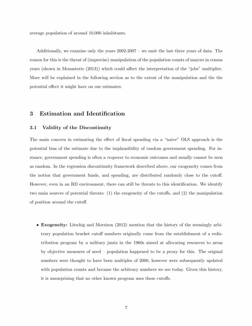
higher spending. Figures 2 and 3 show the jump in the overall receipts, and overall non-finance

government spending 2 (not including state or year fixed effects). Tables 1, 2, and 3 show the

2”Non-Finance refers to spending that is not used to pay off loans or debts for, say, past projects. ”Finance”

spending is a small fraction of overall spending and does not jump at the cutoffs. For our intents, non-finance spending

9

numerical estimates of the jump. On average, receipts and spending both seem to rise by about

11%-13%.

4 Results

Given our first stage, we show both the reduced form and instrumental variable estimates, which

use place above the cutoff to generate plausibly exogenous increases in spending that can be used

to determine the effect of spending on labor market outcomes. This approach is in the vein of the

‘fuzzy’ RD design estimate (Lee and Lemieux (2009)).

4.1 Employment

First stage estimates point to increases in overall jobs by slightly over 210 at the cutoff, seen in

Table 4. Instrumental variables estimates (in Table 8) indicate that a 1% increase in spending is

associated with an 0.92 % increase in the number jobs for a ”spending-employment” elasticity of

close to 1. In table 9, we find an “overall” jobs multiplier of about 0.165 jobs per 1000 reais spent

(in year 2000 reais), or a cost of about $4800 per job in current US dollars. For comparison, Wilson

(2009) estimates a cost of around $125,000 per job, and Serrato and Wingender (2014) estimate

the same to be around $35,000.

This increase in jobs seems to be concentrated in certain skill segments of the labor market,

as shown in the reduced form effects of Table 6. Specifically, the employment increases seem to

be those without college degrees. Jobs involving college educated workers increase almost negligi-

bly, while jobs involving those without a secondary diploma and those who only have a secondary

diploma as their highest education level increase by around 160 and 50 respectively, accounting for

nearly all of the increase in overall jobs.

There also seems to be heterogeneity across sectors of the labor market (Table 7). Private

will be henceforth referred to as ”general spending.”

10

employment increases significantly, and there seems to be a reduction in the number of municipal

jobs, though the effect is not precisely estimated. As crowd-out of private sector labor is often

a concern in fiscal spending studies, it seems that there is no evidence of this but rather some

indication that there may be some “reverse” crowd-out occurring.

4.2 Earnings and Wages

Earnings data is available from the RAIS at the monthly level, however, we so far have not able to

identify consistent effects of spending on wages. Point estimates tended to be small and insignifi-

cant, as shown in Table 5. Given the rigid nature of wage setting in Brazil, this result is perhaps

unsurprising.

5 Discussion

There are several potential explanations for why we might see large job effects concentrated among

the lower skilled and the private sector. Firstly, municipalities may be engaging in public works

projects that require the use of external, low-skilled (and perhaps temporary) labor. If this is true,

then it is debatable to what extent these job numbers can be considered real ’contributions’ to

the economy. To the extent these workers are taken from the unemployed, it could potentially be

hugely beneficial; however, if the workers are coming from outside the municipality and will return

to their place of permanent residence, then the long-run effect may be negligible. More work to

determine the effects of worker relocation is needed to definitively answer this question.

Secondly, it is known that firing public workers in Brazil is notoriously hard due to legal con-

straints. Mayors and other employers, conditional on the eventual receipt of government funds,

may therefore have an incentive to hire labor on contracts which may be more easily dissolved.

However, aside from these concerns, our results indicate that public spending in Brazil may

indeed have some redistributive qualities at the local level. Household income has been linked to

11

skill-level, and to the extent that jobs are being created among the lower-skilled segment of the

labor force, government spending could represent a transfer to lower-income households, which may

exist independently of social welfare programs like Bolsa Familia.

6 Conclusion

Overall, we find evidence of sizable employment effects from local government spending in Brazil.

Using a discontinuity in the allocation of federal transfers according to population brackets, we find

that the effect is concentrated at the lower end of the skill distribution – virtually no jobs involving

workers with college education were created. Additionally, there appears to be evidence that the

effect is also concentrated within the private sector. Surprisingly, public sector jobs did not see an

increase as a result of being just above the cutoff.

Our results point to the notion that ‘jobs multipliers’ in developing countries may be large due

to the hiring of low-skilled labor. To the extent that skill level is correlated with household income,

our results indicate that government spending may have a potential redistributive effect. More

work remains to be done on the effects on wages and on the trajectory of individual workers as

they face an economy with higher levels of spending.

12

References

[1] Algan, Yann, Pierre Cahuc, and Andre Zylberberg (2002). ”Public Employment and Labor

Market Performances”. Economic Policy:1-65.

[2] Barro, Robert (1981). ”Output Effects of Government Purchases.” Journal of Political Economy.

89: 1086 - 1121.

[3] Behar, Alberto and Junghwan Mok (2013). ”Does Public-Sector Employment Fully Crowd-out

Private-Sector Employment?” IMF Working Paper 13/146.

[4] Blanchard, Olivier and Roberto Perotti (2002). ”An Empirical Characterization of the Dynamic

Effects of Changes in Government Spending. Quarterly Journal of Economics. 117(4): 1329-

1368.

[5] Brollo, Fernanda, Tommaso Nannicini, Roberto Perotti, and Guido Tabellini (2012). ”The

Political Resource Curse”.

[6] Caselli, Francesco and Guy Michaels (2013). ”Do Oil Windfalls Improve Living Standards?

Evidence from Brazil”. American Economic Journal: Applied Economics 5(1): 208-38.

[7] Ferraz, Claudio, and Frederico Finan (2008). ”Exposing Corrupt Politicians: The Effects of

Brazil’s Publicly Released Audits on Electoral Outcomes.” Quarterly Journal of Economics 123

(3): 703745.

[8] Gyimah-Brempong, Kwabena (2002). ”Corruption, Economic Growth, and Income Inequality

in Africa.” Economics of Governance 3: 183-209.

[9] Kraay, Aart (2012). ”How Large is the Government Spending Multiplier? Evidence from World

Bank Lending”. Quarterly Journal of Economics. 127(2): 829-887.

[10] Kraay, Aart (2013). ”Government Multipliers in Developing Countries: Evidence from Lending

by Official Creditors”.

[11] Mauro, Paolo (1995). ”Corruption and Growth.” Quarterly Journal of Economics. 110(3): 681

- 712.

13

[12] Lee, David and Thomas Lemieux (2010). ”Regression Discontinuity Designs in Economics”.

Journal of Economic Literature. 48(2): 281-355.

[13] Litschig, Stephan (2012). ”Are Rules-based Government Programs Shielded from Special-

Interest Politics? Evidence from Revenue-Sharing Transfers in Brazil”. Journal of Public Eco-

nomics. 96: 1047-1060.

[14] Litschig, Stephan, and Kevin Morrison (2012). ”Government Spending and Re-election: Quasi-

Experimental Evidence from Brazilian Municipalities”. Barcelona GSE Working Paper Series.

No. 515.

[15] Monasterio, Leonardo (2013). ”O FPM e a estranha distribuicao da populacao dos pequenos

municipıos brasileiros”. IPEA Texto Para Discussao. No. 1818.

[16] McCrary, Justin (2008). ”Manipulation of the Running Variable in the Regression Discontinu-

ity Design: A Density Test”. Journal of Econometrics. 142(2).

[17] Olken, Benjamin (2007). ”Monitoring Corruption: Evidence from a Field Experiment in In-

donesia”. Journal of Political Economy. 115(2).

[18] Shoag, Daniel (2010). ”The Impact of Government Spending Shocks: Evidence on the Multi-

plier from Public Pension Plan Returns”.

[19] Serrato, Juan Carlos Suarez and Philippe Wingender (2011). ”Estimating the incidence of

government spending”.

[20] Wei, Shang-Jin. ”Corruption in Economic Development: Beneficial Grease, Minor Annoyance,

or Major Obstacle?” Policy Research Working Paper 2048, World Bank.

14

Figure 1: FPM Population Brackets and Corresponding Coefficients

1616

.05

16.1

16.1

516

.216

.25

Ln(G

ener

al R

ecei

pts)

-1500 -1000 -500 0 500 1000 1500Population - Threshold

Figure 2: Ln(General Receipts) as a Function of Normalized Population

15

1616

.05

16.1

16.1

516

.216

.25

Ln(G

ener

al E

xpen

ditu

re)


Figure 3: Ln(General Expenditure) as a Function of Normalized Population

16

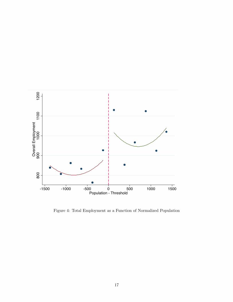
800

900

1000

1100

1200

Ove

rall E

mpl

oym

ent


Figure 4: Total Employment as a Function of Normalized Population

17

(1) (2) (3)

VARIABLES Ln(FPM Transfers) Ln(FPM Transfers) Ln(FPM Transfers)

Above 0.232*** 0.224*** 0.224***

(0.0393) (0.0386) (0.0389)

Observations 2,818 2,818 2,818

R2 0.174 0.250 0.251

State FE NO YES YES

Year FE YES YES YES

Poly. Degree 2 2 2

Flex Slopes YES YES YES

Baseline Controls NO NO YES

Clustered SE Municipality Municipality Municipality

Robust standard errors in parentheses

*** p<0.01, ** p<0.05, * p<0.1

Table 1: Reduced Form Effects on FPM Transfers (in 1000’s of year 2000 reais)

18

(1) (2) (3)

VARIABLES Ln(General Receipts) Ln(General Receipts) Ln(General Receipts)

Above 0.123*** 0.140*** 0.140***

(0.0470) (0.0295) (0.0277)


R2 0.208 0.551 0.585

State FE NO YES YES

Year FE YES YES YES

Poly. Degree 2 2 2





*** p<0.01, ** p<0.05, * p<0.1

Table 2: Reduced Form Effects on Receipts (in 1000’s of year 2000 reais)

19

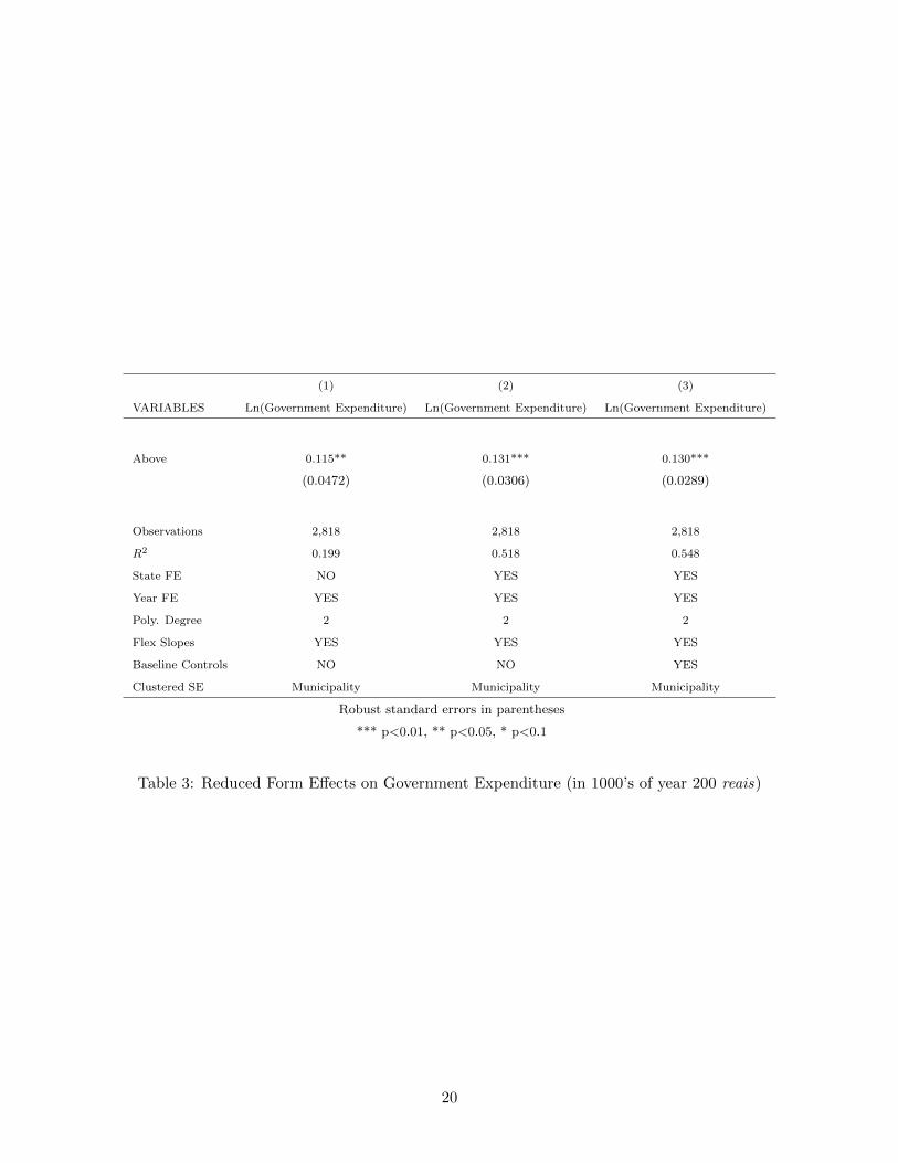
(1) (2) (3)

VARIABLES Ln(Government Expenditure) Ln(Government Expenditure) Ln(Government Expenditure)

Above 0.115** 0.131*** 0.130***

(0.0472) (0.0306) (0.0289)


R2 0.199 0.518 0.548

State FE NO YES YES

Year FE YES YES YES

Poly. Degree 2 2 2





*** p<0.01, ** p<0.05, * p<0.1

Table 3: Reduced Form Effects on Government Expenditure (in 1000’s of year 200 reais)

20

(1) (2) (3)

VARIABLES Overall Employment Overall Employment Overall Employment

Above 147.8 226.7** 217.8**

(119.9) (108.4) (94.43)


R2 0.008 0.179 0.286

State FE NO YES YES

Year FE YES YES YES

Poly. Degree 2 2 2





*** p<0.01, ** p<0.05, * p<0.1

Table 4: Reduced Form Effects on Total Employment (Number of Jobs)

21

(1) (2) (3)

VARIABLES Ln Avg. Wage Ln Avg. Wage Ln Avg. Wage

Above -0.0329 0.0202 0.0188

(0.0460) (0.0304) (0.0313)


R2 0.075 0.447 0.465

State FE NO YES YES

Year FE YES YES YES

Poly. Degree 2 2 2





*** p<0.01, ** p<0.05, * p<0.1

Table 5: Reduced Form Effects on Ln(Average Monthly Earnings)

22

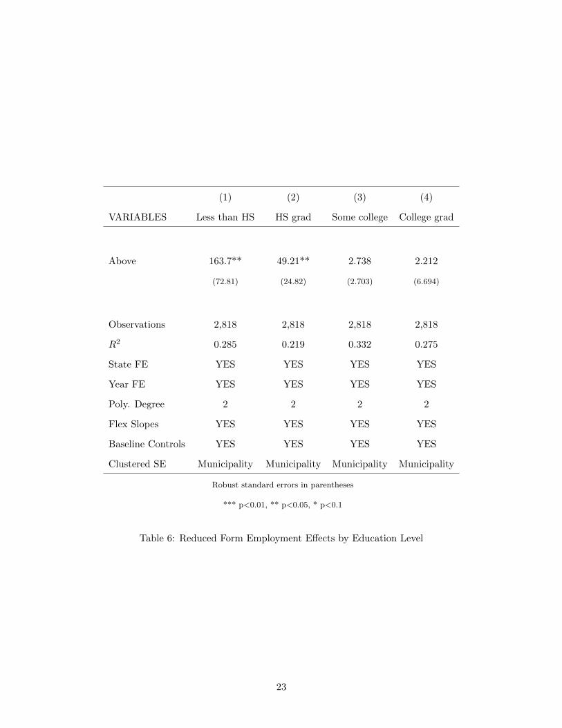
(1) (2) (3) (4)

VARIABLES Less than HS HS grad Some college College grad

Above 163.7** 49.21** 2.738 2.212

(72.81) (24.82) (2.703) (6.694)

Observations 2,818 2,818 2,818 2,818

R2 0.285 0.219 0.332 0.275

State FE YES YES YES YES

Year FE YES YES YES YES

Poly. Degree 2 2 2 2

Flex Slopes YES YES YES YES

Baseline Controls YES YES YES YES

Clustered SE Municipality Municipality Municipality Municipality


*** p<0.01, ** p<0.05, * p<0.1

Table 6: Reduced Form Employment Effects by Education Level

23

(1) (2) (3)

VARIABLES Private Public - Municipal Public - Other

Above 226.2** -11.17 0.875*

(89.99) (16.12) (0.521)


R2 0.241 0.281 0.026

State FE YES YES YES

Year FE YES YES YES

Poly. Degree 2 2 2


Baseline Controls YES YES YES



*** p<0.01, ** p<0.05, * p<0.1

Table 7: Reduced Form Employment Effects by Sector

24

(1) (2)

VARIABLES Ln(Government Expenditure) Ln Employment

Above 0.130***

(0.0289)

Ln(Government Expenditure) 0.918*

(0.507)

Constant 15.40*** -10.60

(0.201) (7.826)

Observations 2,818 2,818

R2 0.548 0.696

State FE YES YES

Year FE YES YES

Poly. Degree 2 2

Flex Slopes YES YES

Baseline Controls YES YES

First Stage F Stat 16.29 16.29

Clustered SE Municipality Municipality


*** p<0.01, ** p<0.05, * p<0.1

Table 8: IV Estimates of Ln(Expenditure) on Ln(Employment)

25

(1) (2)

VARIABLES Gen. Expenditure Overall Employment

Above 1,318***

(326.5)

Gen. Expenditure 0.165**

(0.0745)

Constant 2,779 -2,002***

(2,290) (642.7)

Observations 2,818 2,818

R2 0.496 0.309

State FE YES YES

Year FE YES YES

Poly. Degree 2 2

Flex Slopes YES YES

Baseline Controls YES YES

First Stage F Stat 16.29 16.29

Clustered SE Municipality Municipality


*** p<0.01, ** p<0.05, * p<0.1

Table 9: IV Estimates of Expenditure on Employment

26

Documents

Local Government Spending and Employment in Brazil ... · Local Government Spending and Employment in ... updated by literature attempting to use novel ... nd evidence of a political