Embed Size (px)
Citation preview

Jean-Pierre Ramis
Jacques Sauloy
Changgui Zhang
LOCAL ANALYTICCLASSIFICATION OFq-DIFFERENCE EQUATIONS
Jean-Pierre RamisInstitut de France (Academie des Sciences) and Laboratoire Emile Picard,Institut de Mathematiques, CNRS UMR 5219, U.F.R. M.I.G., UniversitePaul Sabatier (Toulouse 3), 31062 Toulouse CEDEX 9.E-mail : [email protected]
Jacques SauloyLaboratoire Emile Picard, Institut de Mathematiques, CNRS UMR 5219,U.F.R. M.I.G., Universite Paul Sabatier (Toulouse 3), 31062 ToulouseCEDEX 9.E-mail : [email protected]
Url : www.math.univ-toulouse.fr/~sauloy/
Changgui ZhangLaboratoire Paul Painleve, UMR-CNRS 8524, UFR Mathematiques Pures etAppliquees, Universite des Sciences et Technologies de Lille (Lille 1), CiteScientique, 59655 Villeneuve d’Ascq Cedex.E-mail : [email protected]
Url : www-gat.univ-lille1.fr/~zhang/
2000 Mathematics Subject Classification. — 39A13. Secondary:34M50.
Key words and phrases. — q-difference equations, analytic classification,Stokes phenomenon, summation of divergent series.
LOCAL ANALYTIC CLASSIFICATION OFq-DIFFERENCE EQUATIONS
Jean-Pierre Ramis, Jacques Sauloy,Changgui Zhang
Abstract. — We essentially achieve Birkhoff’s program for q-difference equa-tions by giving three different descriptions of the moduli space of isoformal an-alytic classes. This involves an extension of Birkhoff-Guenther normal forms,q-analogues of the so-called Birkhoff-Malgrange-Sibuya theorems and a newtheory of summation. The results were announced in [37, 38] and in variousseminars and conferences between 2004 and 2006.
Resume (Classification analytique locale des equations aux q-differences)
Nous achevons pour l’essentiel le programme de Birkhoff pour la classifica-tion des equations aux q-differences en donnant trois descriptions distinctesde l’espace des modules des classes analytiques isoformelles. Cela passe parune extension des formes normales de Birkhoff-Guenther, des q-analogues destheoremes dits de Birkhoff-Malgrange-Sibuya et une nouvelle theorie de lasommation. Ces resultats ont ete annonces dans [37, 38] ainsi que dans diverssminaires et conferences de 2004 a 2006.


CONTENTS
1. Introduction. . . . . . . . . . . . . . . . . . . . . . . . . . . . . . . . . . . . . . . . . . . . . . . . . . . . . . . . 11.1. The problem. . . . . . . . . . . . . . . . . . . . . . . . . . . . . . . . . . . . . . . . . . . . . . . . . . . . . . 11.2. Contents of the paper. . . . . . . . . . . . . . . . . . . . . . . . . . . . . . . . . . . . . . . . . . . . . 41.3. General notations. . . . . . . . . . . . . . . . . . . . . . . . . . . . . . . . . . . . . . . . . . . . . . . . . 7Acknowledgements. . . . . . . . . . . . . . . . . . . . . . . . . . . . . . . . . . . . . . . . . . . . . . . . . . . . . 9
2. Some general nonsense . . . . . . . . . . . . . . . . . . . . . . . . . . . . . . . . . . . . . . . . . . . . 112.1. The category of q-difference modules. . . . . . . . . . . . . . . . . . . . . . . . . . . . . . 112.2. The Newton polygon and the slope filtration. . . . . . . . . . . . . . . . . . . . . . 152.3. Classification of isograded filtered difference modules. . . . . . . . . . . . . 232.4. The cohomological equation. . . . . . . . . . . . . . . . . . . . . . . . . . . . . . . . . . . . . . . 41
3. The affine space of isoformal analytic classes . . . . . . . . . . . . . . . . . . . 433.1. Isoformal analytic classes of analytic q-difference modules. . . . . . . . . 433.2. Index theorems and irregularity. . . . . . . . . . . . . . . . . . . . . . . . . . . . . . . . . . . 473.3. Explicit description of F(P1, . . . , Pk) in the case of integral slopes 513.4. Interpolation by q-Gevrey classes. . . . . . . . . . . . . . . . . . . . . . . . . . . . . . . . . 56
4. The q-analogs of Birkhoff-Malgrange-Sibuya theorems . . . . . . . . 594.1. Asymptotics. . . . . . . . . . . . . . . . . . . . . . . . . . . . . . . . . . . . . . . . . . . . . . . . . . . . . . 594.2. Existence of asymptotic solutions. . . . . . . . . . . . . . . . . . . . . . . . . . . . . . . . . 654.3. The fundamental isomorphism. . . . . . . . . . . . . . . . . . . . . . . . . . . . . . . . . . . . 694.4. The isoformal classification by the cohomology of the Stokes sheaf 77
5. Summation and asymptotic theory . . . . . . . . . . . . . . . . . . . . . . . . . . . . . . 795.1. Some preparatory notations and results. . . . . . . . . . . . . . . . . . . . . . . . . . . 795.2. Asymptotics relative to a divisor. . . . . . . . . . . . . . . . . . . . . . . . . . . . . . . . . . 855.3. q-Gevrey theorem of Borel-Ritt and flat functions. . . . . . . . . . . . . . . . 955.4. Relative divisors and multisummable functions. . . . . . . . . . . . . . . . . . . 100
vi CONTENTS
5.5. Analytic classification of linear q-difference equations. . . . . . . . . . . . . 104
6. Geometry of the space of classes. . . . . . . . . . . . . . . . . . . . . . . . . . . . . . . . . 1116.1. Privileged cocycles. . . . . . . . . . . . . . . . . . . . . . . . . . . . . . . . . . . . . . . . . . . . . . . . 1116.2. Devissage q-Gevrey. . . . . . . . . . . . . . . . . . . . . . . . . . . . . . . . . . . . . . . . . . . . . . . 1166.3. Vector bundles associated to q-difference modules. . . . . . . . . . . . . . . . . 120
7. Examples of the Stokes phenomenon . . . . . . . . . . . . . . . . . . . . . . . . . . . . 1237.1. The q-Euler equation and confluent basic hypergeometric series. . . 1247.2. The symmetric square of the q-Euler equation. . . . . . . . . . . . . . . . . . . . 1307.3. From the Mock Theta functions to the q-Euler equation. . . . . . . . . . 1357.4. From class numbers of quadratic forms to the q-Euler equation . . . 139
Bibliography. . . . . . . . . . . . . . . . . . . . . . . . . . . . . . . . . . . . . . . . . . . . . . . . . . . . . . . . . . . 143
CHAPTER 1
INTRODUCTION
1.1. The problem
1.1.1. The generalized Riemann problem and the allied problems.— This paper is a contribution to a large program stated and begun by G.D.Birkhoff in the beginning of XXth century [8]: the generalized Riemann prob-lem for linear differential equations and the allied problems for linear differenceand q-difference equations. Such problems are now called Riemann-Hilbert-Birkhoff problems. Today the state of achievement of the program as it wasformulated by Birkhoff in [8]: is the following.
– For linear differential equations the problem is completely closed (bothin the regular-singular case and in the irregular case).
– For linear q-difference equations (|q| 6= 1), taking account of precedingresults due to Birkhoff [8], the second author [44] and van der Put-Reversat [51] in the regular-singular case, and to Birkhoff-Guenther [9]in the irregular case, the present work essentially closes the problem andmoreover answers related questions formulated later by Birkhoff in a jointwork with his PhD student P.E. Guenther [9] (cf. below 1.1.2).
– For linear difference equations the problem is closed for global regular-singular equations (Birkhoff, J. Roques [40]) and there are some impor-tant results in the irregular case [22], [11].
1.1.2. The Birkhoff-Guenther program. — We quote the conclusionof [9], it contains a program which is one of our central motivations for thepresent work. We shall call it Birkhoff-Guenther program.
2 CHAPTER 1. INTRODUCTION
Up to the present time, the theory of q-difference equations has laggednoticeabely behind the sister theories of linear difference and q-differenceequations. In the opinion of the authors, the use of the canonical system,as formulated above in a special case, is destined to carry the theory ofq-difference equations to a comparable degree of completeness. This programincludes in particular the complete theory of convergence and divergence offormal series, the explicit determination of the essential invariants (constantsin the canonical form), the inverse Riemann theory both for the neighborhoodof x = ∞ and in the complete plane (case of rational coefficients), explicitintegral representations of the solutions, and finally the definition of q-sigmaperiodic matrices, so far defined essentially only in the case n = 1. Becauseof its extensiveness this material cannot be presented here.
The paper [9] appeared in 1941 and Birkhoff died in 1944; as far as we know“this material” never appeared and the corresponding questions remainedopened and forgotten for a long time.
1.1.3. What this paper could contain but does not. — Before de-scribing the contents of the paper in the following paragraph, we shall firstsay briefly what it could contain but does not.
The kernel of the present work is the detailed proofs of some resultsannounced in [37], [38] and in various seminars and conferences between 2004and 2006, but there are also some new results in the same spirit and someexamples.
In this paper, we limit ourselves to the case |q| 6= 1. The problem ofclassification in the case |q| = 1 involves diophantine conditions, it remainsopen but for the only exception [15]. Likewise, we do not study problemsof confluence of our invariants towards invariants of differential equations,that is of q-Stokes invariants towards classical Stokes invariants (cf. in thisdirection [17], [55]).
In this work, following Birkhoff, we classify analytically equations admittinga fixed normal form, a moduli problem. There is another way to classifyequations: in terms of representations of a “fundamental group”, in Riemann’sspirit. This is related to the Galois theory of q-difference equations, we willnot develop this topic here, limiting ourselves to the following remarks, even
1.1. THE PROBLEM 3
if the two types of classification are strongly related.
The initial work of Riemann was a “description” of hypergeometric differ-ential equations as two-dimensional representations of the free non-abeliangroup generated by two elements. Later Hilbert asked for a classificationof meromorphic linear differential equations in terms of finite dimensionalrepresentations of free groups. Apparently the idea of Birkhoff was to getclassifications of meromorphic linear differential, difference and q-differenceequations in terms of elementary linear algebra and combinatorics but not interms of group representations. For many reasons it is interesting to work inthe line of Riemann and Hilbert and to translate Birkhoff style invariants interms of group representations. The corresponding groups will be fundamentalgroups of the Riemann sphere minus a finite set or generalized fundamentalgroups. It is possible to define categories of linear differential, difference andq-difference equations, these categories are tannakian categories; then apply-ing the fundamental theorem of Tannakian categories we can interpret themin terms of finite dimensional representations of pro-algebraic groups, theTannakian groups. The fundamental groups and the (hypothetic) generalizedfundamental groups will be Zariski dense subgroups of the Tannakian groups.
In the case of differential equations the work was achieved by the first au-thor, the corresponding group is the wild fundamental group which is Zariskidense in the Tannakian group. In the case of difference equations almostnothing is known. In the case of q-difference equations, the situation is thefollowing.
1. In the local regular singular case the work was achieved by the secondauthor in [45], the generalized fundamental group is abelian, its semi-simple part is abelian free on two generators and its unipotent part isisomorphic to the additive group C.
2. In the global regular singular case only the abelian case is understood[45], using the geometric class field theory. In the general case some nonabelian class field theory is needed.
3. In the local irregular case, using the results of the present paper thefirst and second authors recently got a generalized fundamental group[32, 36, 35].
4. Using case 3, the solution of the global general case should follows easilyfrom the solution of case 2.

4 CHAPTER 1. INTRODUCTION
1.1.3.1. About the asumption that the slopes are integral. — The “abstract”part of our paper does not require any assumption on the slopes: that meansgeneral structure theorems, e.g. theorem 3.1.4 and proposition 3.4.2. Thesame is true of the decomposition of the local Galois group of an irregularequation as a semi-direct product of the formal group by a unipotent groupin [32, 36].
However, all our explicit constructions (Birkhoff-Guenther normal form,privileged cocycles, discrete summation) rest on the knowledge of a normalform for pure modules, that we have found only in the case of integral slopes.
In [51] van der Put and Reversat classified pure modules with non integralslopes. The adaptation of [51] to our results does not seem to have been done- and would be very useful.
1.2. Contents of the paper
We shall classify analytically isoformal q-difference equations. The isofor-mal analytic classes form an affine space, we shall give three descriptions ofthis space respectively in chapters 3, 4 and 6 (this third case is a particularcase of the second and is based upon chapter 5) using different constructionsof the analytic invariants. A direct and explicit comparison between thesecond and the third description is straightforward but such a comparisonbetween the first and the second or the third construction is quite subtle;in the present paper it will be clear for the “abelian case”, of two integralslopes; for the general case we refer the reader to [32, 36] and also to workin progress [48].
Chapter 2 deals with the general setting of the problem (section 2.1) andintroduces two fundamental tools: the Newton polygon and the slope filtra-tion (section 2.2). From this, the problem of analytic isoformal classificationadmits a purely algebraic formulation: the isograded classification of filtereddifference modules. An algebraic theory is developped in section 2.3. Sincethe space under study looks like some generalized extension module, it relieson homological algebra and index computations. Last, in view of dealing withspecific examples, some practical aspects are discussed in section 2.4.
1.2. CONTENTS OF THE PAPER 5
The first attack at the classification problem for q-difference equationscomes in chapter 3. Section 3.1 specializes the results of section 2.3 toq-differences, and section 3.2 provides the proof of some related index com-putations. One finds that the space of classes is an affine scheme (theorem3.1.4) and computes its dimension. This is a rather abstract result. In orderto provide explicit descriptions (normal forms, coordinates, invariants ...)from section 3.3 up to the end of the paper, we assume that the slopes of theNewton polygon are integers. This allows for the more precise theorem 3.3.5and the existence of Birkhoff-Guenther normal forms originating in [9]. Thisalso makes easier the explicit computations of the following chapters. Thensome precisions about q-Gevrey classification are given in section 3.4.
Analytic isoformal classification by normal forms is a special feature ofthe q-difference case, such a thing does not exist for differential equations.To tackle this case Birkhoff introduced functional 1-cochains using Poincareasymptotics [7, 8]. Later, in the seventies, Malgrange interpreted Birkhoffcochains using sheaves on a circle S1 (the real blow up of the origin of thecomplex plane). Here, we modify these constructions in order to deal withthe q-difference case, introducing a new asymptotic theory and replacing thecircle S1 by the elliptic curve Eq = C∗/qZ.
In this spirit, chapter 4 tackles the extension to q-difference equationsof the so called Birkhoff-Malgrange-Sibuya theorems. In section 4.1 is out-lined an asymptotic theory adapted to q-difference equations but weakerthan that of section 5.2 of the next chapter: the difference is the same asbetween classical Gevrey versus Poincare asymptotics. The counterpart ofthe Poincare version of Borel-Ritt is theorem 4.1.4; also, comparison withWhitney conditions is described in lemma 4.1.3. Indeed, the geometric meth-ods of section 4.3 rest on the integrability theorem of Newlander-Niremberg.They allow the proof of the first main theorem, the q-analogue of the abstractBirkhoff-Malgrange-Sibuya theorem (theorem 4.3.10). Then, in section 4.4,it is applied to the classification problem for q-difference equations and oneobtains the q-analogue of the concrete Birkhoff-Malgrange-Sibuya theorem(theorem 4.4.1): there is a natural bijection from the space F(M0) of analyticisoformal classes in the formal class of M0 with the first cohomology setH1(Eq,ΛI(M0)) of the “Stokes sheaf”. The latter is the sheaf of automor-phisms of M0 infinitely tangent to identity, a sheaf of unipotent groups overthe elliptic curve Eq = C∗/qZ. The proof of theorem 4.4.1appeals to the

6 CHAPTER 1. INTRODUCTION
fundamental theorem of existence of asymptotic solutions, previously provedin section 4.2.
Chapter 5 aims at developping a summation process for q-Gevrey divergentseries. After some preparatory material in section 5.1, an asymptotic theory“with estimates” well suited for q-difference equations is expounded in section5.2. Here, the sectors of the classical theory are replaced by preimages inC∗ of the Zariski open sets of the elliptic curve C∗/qZ, that is, complementsof finite unions of discrete q-spirals in C∗; and the growth conditions atthe boundary of the sectors are replaced by polarity conditions along thediscrete spirals. The q-Gevrey analogue of the classical theorems are statedand proved in sections 5.3 and 5.4: the counterpart of the Gevrey versionof Borel-Ritt is theorem 5.3.3 and multisummability conditions appear intheorems 5.4.3 and 5.4.7. The theory is then applied to q-difference equationsand to their classification in section 5.5, where is proved the summability ofsolutions (theorem 5.5.3), the existence of asymptotic solutions coming as aconsequence (theorem 5.5.5) and the description of Stokes phenomenon as anapplication (theorem 5.5.7).
Chapter 6 deals with some complementary information on the geometryof the space F(M0) of analytic isoformal classes, through its identificationwith the cohomology set H1(Eq,ΛI(M0)) obtained in chapter 4. Theorem4.4.1 of chapter 4 implicitly attaches cocycles to analytic isoformal classes andtheorem 5.5.7 of chapter 5 shows how to obtain them by a summation process.In section 6.1, we give yet another construction of “privileged cocycles” (from[46]) and study their properties. In section 6.2, we show how the devissageof the sheaf ΛI(M0) by holomorphic vector bundles over Eq allows to identifyH1(Eq,ΛI(M0)) with an affine space, and relate it to the correspondingresult of theorem 3.3.5. In section 6.3, we recall how holomorphic vectorbundles over Eq appear naturally in the theory of q-difference equations andwe apply them to an interpretation of the formula for the dimension of F(M0).
Chapter 7 provides some elementary examples motivated by their relationto q-special functions, either linked to modular functions or to confluent basichypergeometric series.
It is important to notice that the construction of q-analogs of classical ob-jects (special functions. . . ) is not canonical, there are in general several “good”
1.3. GENERAL NOTATIONS 7
q-analogs. So there are several q-analogs of the Borel-Laplace summation(and multisummation): there are several choices for Borel and Laplace kernels(depending on a choice of q-analog of the exponential function) and severalchoices of the integration contours (continuous or discrete in Jackson style)[34], [39], [53, 56, 54]. Our choice of summation here seems quite ”optimal”:the entries of our Stokes matrices are elliptic functions (cf. the “q-sigma peri-odic matrices” of Birkhoff-Guenther program), moreover Stokes matrices aremeromorphic in the parameter of “q-direction of summation”; this is essentialfor applications to q-difference Galois theory (cf. [32, 36, 35]). Unfortunatelywe did not obtain explicit integral formulae for this summation (except forsome particular cases), in contrast with what happens for other summationsintroduced before by the third author.
1.3. General notations
Generally speaking, in the text, the sentence A := B means that the termA is defined by formula B. But for some changes, the notations are the sameas in [37], [38], etc. Here are the most useful ones.
We write Cz the ring of convergent power series (holomorphic germs at0 ∈ C) and C(z) its field of fractions (meromorphic germs). Likewise, wewrite C[[z]] the ring of formal power series and C((z)) its field of fractions.
We fix once for all a complex number q ∈ C such that |q| > 1. Then, thedilatation operator σq is an automorphism of any of the above rings and fields,well defined by the formula:
σqf(z) := f(qz).
Other rings and fields of functions on which σq operates will be introducedin the course of the paper. This operator also acts coefficientwise on vectors,matrices. . . over any of these rings and fields.
We write Eq the complex torus (or elliptic curve) Eq := C∗/qZ
and p : C∗ → Eq the natural projection. For all λ ∈ C∗, we write[λ; q] := λqZ ⊂ C∗ the discrete logarithmic q-spiral through the point λ ∈ C∗.All the points of [λ; q] have the same image λ := p(λ) ∈ Eq and we mayidentify [λ; q] = p−1
(λ)
with λ.

8 CHAPTER 1. INTRODUCTION
A linear analytic (resp. formal) q-difference equation (implicitly: at 0 ∈ C)is an equation:
(1) σqX = AX,
where A ∈ GLn(C(z)) (resp. A ∈ GLn(C((z)))).
1.3.1. Theta Functions. — Jacobi theta functions pervade the theory of q-difference equations. We shall mostly have use for two slightly different formsof them. In section 5, we shall use:
(2) θ(z; q) :=∑n∈Z
q−n(n−1)/2zn =∏n∈N
(1− q−n−1)(1 + q−nz)(1 + q−n−1/z).
The second equality is Jacobi’s celebrated triple product formula. When ob-vious, the dependency in q will be omitted and we shall write θ(z) instead ofθ(z; q). One has:
θ(qz) = q z θ(z) and θ(z) = θ(1/qz).
In section 7, we shall rather use:
(3) θq(z) :=∑n∈Z
q−n(n+1)/2zn =∏n∈N
(1− q−n−1)(1 + q−n−1z)(1 + q−n/z).
One has of course θq(z) = θ(q−1z; q) and:
θq(qz) = zθq(z) = θq(1/z).
Both functions are analytic over the whole of C∗ and vanish on the discreteq-spiral −qZ with simple zeroes.
1.3.2. q-Gevrey levels. — As in [6],[33], we introduce the space of formalseries of q-Gevrey order s:
C[[z]]q;s :=∑
anzn ∈ C[[z]] | ∃A > 0 : fn = O
(Anqsn2/2
).
We also say that f ∈ C[[z]]q;s is of q-Gevrey level 1/s. It understood thatC[[z]]0 = Cz and C[[z]]∞ = C[[z]] (but it is not true that
⋂s>0
C[[z]]s =
Cz, nor that⋃
s>0C[[z]]s = C[[z]]).
Similar considerations apply to spaces of Laurent formal series:
C((z))q;s := C[[z]]q;s[1/z].
More generally, one can speak of q-Gevrey sequences of complex numbers. Let
k ∈ R∗ ∪ ∞ and s :=1k
. A sequence (an) ∈ CN is q-Gevrey of order s if it
is dominated by a sequence of the form(CAn |q|n
2/(2k))
, for some constants

ACKNOWLEDGEMENTS 9
C,A > 0.Note that this terminology is all about sequences, or coefficients of series.Extension to q-Gevrey asymptotics is explained in definition 5.2.1, while the q-Gevrey interpolation by growth of decay of functions is dealt with in definitions5.2.7 and 5.4.1.
Acknowledgements
During the final redaction of this work, the first author beneffited of asupport of the ANR Galois (Programme Blanc) and was invited by the de-partement of mathematics of Tokyo University (College of Arts and Science,Komaba). During the same period, the second author benefitted of a semesterCRCT by the Universite Toulouse 3 and was successively invited by Universityof Valladolid (Departamento de Algebra, Geometria and Topologia), Univer-site des Sciences et Technologies de Lille (Laboratoire Paul Painleve) and Insti-tut Mathematique de Jussieu (Equipe de Topologie et Geometrie Algebriques);he wants to thank warmly these three departments for their nice working at-mosphere. Last, we heartily thank the referee of prevous submissions of thispaper, who encouraged us to add some motivating examples (these make upthe contents of chapter 7) and to extend it to the presentn form.

CHAPTER 2
SOME GENERAL NONSENSE
2.1. The category of q-difference modules
General references for this section are [52], [47]
2.1.1. Some general facts about difference modules. — Here, we alsorefer to the classical litterature about difference fields, like [13] and [18] (seealso [31]). We shall also use specific results proved in section 2.3.
We call difference field (1) a pair (K,σ), where K is a (commutative) fieldand σ a field automorphism of K. We write indifferently σ(x) or σx the actionof σ on x ∈ K. One can then form the Ore ring of difference operators:
DK,σ := K〈T, T−1〉
characterized by the twisted commutation relation:
∀k ∈ Z , x ∈ K , T kx = σk(x)T k.
We shall rather write somewhat improperly DK,σ := K〈σ, σ−1〉 and, for short,D := DK,σ in this section. The center of D is the “field of constants”:
Kσ := x ∈ K | σ(x) = x.
The ring D is left euclidean and any ideal is generated by an entire unitarypolynomial P = σn + a1σ
n−1 + · · · + an, but such a generator is by no waysunique. For instance, it is an easy exercice to show that σ − a and σ − a′(with a, a′ ∈ K∗) generate the same ideal if, and only if, a′/a belongs to the
(1)Much of what follows will be extended to the case of difference rings in section 2.3, where
the basic linear constructions will be described in great detail.
12 CHAPTER 2. SOME GENERAL NONSENSE
subgroup σbb | b ∈ K
∗ of K∗.
Any (left) D-module M ∈ ModD can be seen as a K-vector space E andthe left multiplication x 7→ σ.x as a semi-linear automorphism Φ : E → E,which means that Φ(λx) = σ(λ)Φ(x); and any pair (E,Φ) of a K-vector spaceE and a semi-linear automorphism Φ of E defines a D-module; we just writeM = (E,Φ). Morphisms from (E,Φ) to (E′,Φ′) in ModD are linear mapsu ∈ LK(E,E′) such that Φ′ u = u Φ.
The D-module M has finite length if, and only if, E is a finite dimensionalK-vector space. A finite length D-module is called a difference module over(K,σ), or over K for short. The full subcategory of ModD whose objects areof difference modules is written DiffMod(K,σ). The categories ModD andDiffMod(K,σ) are abelian and Kσ-linear.
By choosing a basis of E, we can identify any difference module with some(Kn,ΦA), where A ∈ GLn(K) and ΦA(X) := A−1σX (with the natural op-eration of σ on Kn); the reason for using A−1 will become clear soon. IfB ∈ GLp(K), then morphisms from (Kn,ΦA) to (Kp,ΦB) can be identi-fied with matrices F ∈ Matp,n(K) such that (σF )A = BF (and compositionamounts to the product of matrices).
2.1.1.1. Unity. — An important particular object is the unity 1, which maybe described either as (K,σ) or as D/DP with P = σ − 1. For any differencemodule M = (E,Φ) the Kσ-vector space Hom(1,M) can be identified withthe kernel of the Kσ-linear map Φ − Id : E → E; in case M = (Kn,ΦA),this boils down to the space X ∈ Kn | σX = AX of solutions of a “σ-difference system”; whence our definition of ΦA. The functor of solutionsM ; Γ(M) := Hom(1,M) is left exact and Kσ-linear. We shall have use ofits right derived functors Γi(M) = Exti(1,M) (see [10]).
2.1.1.2. Internal Hom. — Let M = (E,Φ) and N = (E,Ψ). The map TΦ,Ψ :f 7→ ΨfΦ−1 is a semi-linear automorphism of the K-vector space LK(E,F ),whence a difference module Hom(M,N) :=
(LK(E,F ), TΦ,Ψ
). Then one has
Hom(1,M) = M and Γ(Hom(M,N)
)= Hom(M,N). The dual of M is
M∨ := Hom(M, 1), so that Hom(M, 1) = Γ(M∨). For instance, the dual ofM = (Kn,ΦA) is M∨ = (Kn,ΦA∨), where A∨ := tA−1.

2.1. THE CATEGORY OF q-DIFFERENCE MODULES 13
2.1.1.3. Tensor product. — Let M = (E,Φ) and N = (E,Ψ). The mapΦ⊗Ψ : x⊗y 7→ Φ(x)⊗Ψ(y) from E⊗KF to itself is well defined and it is a semi-linear automorphism, whence a difference module M ⊗N = (E⊗K F,Φ⊗Ψ).The obvious morphism yields the adjunction relation:
Hom(M,Hom(N,P )
)= Hom(M ⊗N,P ).
We also have functorial isomorphisms 1⊗M = M and Hom(M,N) = M∨⊗N .The classical computation of the rank through 1 → M∨ ⊗ M → 1 yieldsdimK E as it should. We write rk M this number.
2.1.1.4. Extension of scalars. — An extension difference field (K ′, σ′) of(K,σ) consists in an extension K ′ of K and an automorphism σ′ of K ′ whichrestricts to σ on K. Any difference module M = (E,Φ) over (K,σ) then givesrise to a difference module M ′ = (E′,Φ′) over (K ′, σ)′, where E′ := K ′ ⊗L E
and Φ′ := σ′ ⊗ Φ is defined the same way as above. We then write ΓK′(M)the K ′σ′-vector space Γ(M ′). The functor of solutions (with values) inK ′ M ; Γ(M ′) = Hom(1,M ′) is left exact and Kσ-linear. The functorM ; M ′ from DiffMod(K,σ) to DiffMod(K ′, σ′) is compatible withunity, internal Hom, tensor product and dual. The image of M = (Kn,ΦA)is M ′ = (K ′n,ΦA).
2.1.2. q-difference modules. — We now restrict our attention to the dif-ference fields
(C(z), σq
)and
(C((z)), σq
), and to the corresponding cate-
gories of analytic, resp. formal, q-difference modules: they are C-linear abeliancategories since C(z)σq = C((z))σq = C. In both settings, we consider theq-difference module M = (Kn,ΦA) as an abstract model for the linear q-difference system σqX = AX. Isomorphisms from (the system with matrix)A to (the system with matrix) B in either category correspond to analytic,resp. formal, gauge transformations, i.e. matrices F ∈ GLn(C(z)), resp.F ∈ GLn(C((z))), such that B = F [A] := (σqF )AF−1. We write Dq indiffer-ently for DC(z),σq
or DC((z)),σqwhen the distinction is irrelevant.
Lemma 2.1.1 (Cyclic vector lemma). — Any (analytic or formal) q-difference module is isomorphic to a module Dq/DqP for some unitary entireq-difference operator P .
Proof. — See [14], [44].
Theorem 2.1.2. — The categories DiffMod(C(z), σq) and DiffMod(C((z)), σq)are abelian C-linear rigid tensor categories. (They actually are neutral tan-nakian categories, but we won’t use this fact.)

14 CHAPTER 2. SOME GENERAL NONSENSE
Proof. — See [52], [45].
2.1.2.1. The functor of solutions. — It is customary in D-module theory tocall solution of M a morphism M → 1. Indeed, a solution of D/DP is then anelement of Ker P . We took the dual convention, yielding a covariant C-linearleft exact functor Γ for the following reason. To any analytic q-differencemodule M = (C(z)n,ΦA), one can associate a holomorphic vector bundleFA over the elliptic curve (or complex torus) Eq := C∗/qZ in such a way thatthe space of global sections of FA can be identified with Γ(M). We thus thinkof Γ as a functor of global sections, and, the functor M ; FA being exact,the Γi can be defined through sheaf cohomology.
There is an interesting relationship between the space Γ(M) = Hom(1,M)of solutions of M and the space Γ(M∨) = Hom(M, 1) of “cosolutions” ofM . Starting from a unitary entire (analytic or formal) q-difference operatorP = σn
q + a1σn−1q + · · ·+ an ∈ Dq, one studies the solutions of the q-difference
equation:P.f := σn
q f + a1σn−1q f + · · ·+ anf = 0
by vectorializing it into the form:
σqX = AX, where X =
f
σqf...
σn−2q f
σn−1q f
and A =
0 1 0 . . . 00 0 1 . . . 0...
......
. . ....
0 0 0 . . . 1−an −an−1 −an−2 − . . . −a1
.
Solutions of P then correspond to solutions of M = (C(z)n,ΦA) or(C((z))n,ΦA). Now, by lemma 2.1.1, one has M = Dq/DqQ for some unitaryentire q-difference operator Q. Any such polynomial Q is dual to P . Anexplicit formula for a particular dual polynomial is given in [47].
From the derived functors Γi(M) = Exti(1,M), one can recover generalExt-modules:
Proposition 2.1.3. — There are functorial isomorphisms:
Exti(M,N) ' Γi(M∨ ⊗N).
Proof. — The covariant functor N ; Hom(M,N) is obtained by composingthe exact covariant functor N ; M∨⊗N with the left exact covariant functorΓ. One can then derive it using [20], chap. III, §7, th. 1, or directly by

2.2. THE NEWTON POLYGON AND THE SLOPE FILTRATION 15
writing down a right resolution of Γ and applying the exact functor, then thecohomology sequence of Γ.
Remark 2.1.4. — For any difference field extension (K,σ) of (C(z), σq),the Kσ-vector space of solutions of M in K has dimension dimKσ ΓK(M) ≤rk M : this follows from the q-wronskian lemma (see [14]). One can showthat the functor ΓK is a fibre functor if, and only if, (K,σ) is a universalfield of solutions, i.e. such that one always have the equality dimKσ ΓK(M) =rk M . The field M(C∗) of meromorphic functions over C∗, with the auto-morphism σq, is a universal field of solutions, thus providing a fibre functorover M(C∗)σq = M(Eq) (field of elliptic functions). Actually, no subfieldof M(C∗) gives a fibre functor over C (see [45]). In [52], van der Put andSinger use an algebra of symbolic solutions which is reduced but not integral.A transcendental construction of a fibre functor over C is described in [32].
2.2. The Newton polygon and the slope filtration
We summarize results from [47] (2).
2.2.1. The Newton polygon. — The contents of this section are valid aswell in the analytic as in the formal setting. To the (analytic or formal) q-difference operator P =
∑aiσ
iq ∈ Dq, we associate the Newton polygon N(P ),
defined as the convex hull of (i, j) ∈ Z2 | j ≥ v0(ai), where v0 denotes thez-adic valuation in C(z),C((z)). Multiplying P by a unit aσk
q of Dq justtranslates the Newton polygon by a vector of Z2, and we shall actually considerN(P ) as defined up to such a translation (or, which amounts to the same,choose a unitary entire P ). The relevant information therefore consists in thelower part of the boundary of N(P ), made up of vectors (r1, d1), . . . , (rk, dk),
ri ∈ N∗, di ∈ Z. Going from left to right, the slopes µi :=di
riare rational
numbers such that µ1 < · · · < µk. Their set is written S(P ) and ri is themultiplicity of µi ∈ S(P ). The most convenient object is however the Newtonfunction rp : Q→ N, such that µi 7→ ri and null out of S(P ).
(2)Note however that, from [32], we changed our terminology: the slopes of a q-difference
module are the opposites of what they used to be; and what we call a pure isoclinic (resp.
pure) module was previously called pure (resp. tamely irregular).
16 CHAPTER 2. SOME GENERAL NONSENSE
Theorem 2.2.1. — (i) For a given q-difference module M , all unitary entireP such that M ' Dq/DqP have the same Newton polygon; the Newton polygonof M is defined as N(M) := N(P ), and we put S(M) := S(P ), rM := rP .(ii) The Newton polygon is additive: for any exact sequence,
0→M ′ →M →M ′′ → 0 =⇒ rM = rM ′ + rM ′′ .
(iii) The Newton polygon is multiplicative:
∀µ ∈ Q , rM1⊗M1(µ) =∑
µ1+µ2=µ
rM1(µ1)rM2(µ2).Also: rM∨(µ) = rM (−µ).
(iv) Let ` ∈ N∗, introduce a new variable z′ := z1/` (ramification) and makeK ′ := C((z))[z′] = C((z′)) or C(z)[z′] = C(z′) a difference field extensionby putting σ′(z′) = q′z′, where q′ is any `th root of q. The Newton polygon ofthe q′-difference module M ′ := K ′ ⊗M (computed w.r.t. variable z′) is givenby the formula:
rM (µ) = rM ′(`µ).
Example 2.2.2. — Vectorializing an analytic equation of order two yields:
σ2qf+a1σqf+a2f = 0⇐⇒ σqX = AX, with X =
(f
σqf
)and A =
(0 1−a2 −a1
).
The associated module is (C(z)2,ΦA). Putting e :=(
10
), one has ΦA(e) =(
−a1/a2
1
)and:
Φ2A(e) =
−1a2e+−σqa1
σqa2ΦA(e) =⇒M ' Dq/DqL, where L := σ2
q +σqa1
σqa2σq+
1a2,
L thus being a dual of L. Note that if we started from vector e′ :=(
01
), we
would compute likewise:
Φ2A(e′) =
−1σqa2
e′+−a1
σqa2ΦA(e′) =⇒M ' Dq/DqL′, where L′ := σ2
q+a1
σqa2σq+
1σqa2
,
another dual of L. However, they give the same Newton polygon, sincev0(a1/σqa2) = v0(σqa1/σqa2) and v0(1/σqa2) = v0(1/a2).We now specialize to the equation satisfied by a q-analogue of the Euler series,the so-called Tshakaloff series:
(4) Ch(z) :=∑n≥0
qn(n−1)/2zn.

2.2. THE NEWTON POLYGON AND THE SLOPE FILTRATION 17
Then φ := Ch satisfies:
φ = 1 + zσqφ =⇒ L.φ = 0,
where:
qzL := (σq − 1)(zσq − 1) = qzσ2q − (1 + z)σq + 1.
By our previous definitions, S(L) = 0, 1 (both multiplicities equal 1). Thesecond computation of a dual above implies that:
M ' Dq/DqP, where P := σ2q − q(1 + z)σq + q2z = (σq − qz)(σq − q),
whence S(M) = S(P ) = −1, 0 (both multiplicities equal 1).This computation relies on the obvious vectorialisation with matrix A =(
0 1−1/qz (1 + z)/qz
). However, we also have:
L.f = 0⇐⇒ σqY = BY, with X =(
f
zσqf − f
)and B =
(z−1 z−1
0 1
).
The fact that matrix A is analytically equivalent to an upper triangular matrixcomes from the analytic factorisation of L; the exponents of z on the diagonalare the slopes: this, as we shall see, is a general fact when the slopes areintegral.
2.2.2. Pure modules. — We call pure isoclinic (of slope µ) a module Msuch that S(M) = µ and pure a direct sum of pure isoclinic modules. Wecall fuchsian a pure isoclinic module of slope 0. The following description isvalid whether K = C((z)) or C(z).
Lemma 2.2.3. — (i) A pure isoclinic module of slope µ over K can be writ-ten:
M ' Dq/DqP, where P = anσnq + an−1σ
n−1q + · · ·+ a0 ∈ Dq with :
a0an 6= 0 ; ∀i ∈ 1, n− 1 , v0(ai) ≥ v0(a0) + µi and v0(an) = v0(a0) + µn.
(ii) If µ ∈ Z, it further admits the following description:
M = (Kn,ΦzµA) with A ∈ GLn(C).
Proof. — The first description is immediate from the definitions. The secondis proved in [47].

18 CHAPTER 2. SOME GENERAL NONSENSE
2.2.2.1. Pure modules with integral slopes. — In particular, any fuchsian mod-ule is equivalent to some module (Kn,ΦA) with A ∈ GLn(C). One maymoreover require that A has all its eigenvalues in the fundamental annulus:
∀λ ∈ SpA , 1 ≤ |λ| < |q| .
Last, two fuchsian modules (Kn,ΦA), (Kn′ ,ΦA′) with A ∈ GLn(C),A′ ∈ GLn′(C) having all their eigenvalues in the fundamental annulusare isomorphic if and only if the matrices A,A′ are similar (so that n = n′).
It follows that any pure isoclinic module of slope µ is equivalent to somemodule (Kn,ΦzµA) with A ∈ GLn(C), the matrix A having all its eigen-values in the fundamental annulus; and that two such modules (Kn,ΦzµA),(Kn′ ,ΦzµA′) are isomorphic if and only if the matrices A,A′ are similar.
2.2.2.2. Pure modules of arbitrary slopes. — The classification of pure mod-ules of arbitrary (not necessarily integral) slopes was obtained by van derPut and Reversat in [51]. It is cousin to the classification by Atiyah ofvector bundles over an elliptic curve, which it allows to recover in a sim-ple and elegant way. Although we shall not need it, we briefly recall that result.
The first step is the classification of irreducible (that is, simple) modules.An irreducible q-difference module M is automaticaly pure isoclinic of slopesay µ. We write µ = d/r with d, r coprime and may assume that r ≥ 2 (thecase r = 1 is already known). Let K ′ := K[z1/r] = K[z′] and q′ an arbitraryrth root of q. Then M is isomorphic to the restriction of some q′-differencemodule M ′ of rank 1 over K ′; and M ′ is isomorphic to (K ′,Φcz′d) for a uniquec ∈ C∗ such that 1 ≤ |c| < |q′|. Actually:
M ' E(r, d, cr) := Dq/Dq
(σr
q − q′−dr(r−1)/2
c−rz−d).
Moreover, for E(r, d, a) and E(r′, d′, a′) to be isomorphic, it is necessary (andsufficient) that (r′, d′, a′) = (r, d, a).
Then van der Put and Reversat prove that an indecomposable moduleM (that is, M is not a non trivial direct sum) comes from successive ex-tensions of isomorphic irreducible modules; indeed, it has the form M 'E(r, d, a)⊗ (Km,ΦU ) for some indecomposable unipotent constant matrix U .Last, any pure isoclinic module is a direct sum of indecomposable modules inan essentially unique way.

2.2. THE NEWTON POLYGON AND THE SLOPE FILTRATION 19
2.2.3. The slope filtration. — Submodules, quotient modules, sums. . . ofpure isoclinic modules of a given slope keep the same property. It follows thateach module M admits a biggest pure submodule M ′ of slope µ; one then hasa priori rk M ′ ≤ rM (µ). Like in the case of differential equations, one wantsto “break the Newton polygon” and find pure submodules of maximal possiblerank. In the formal case, the results are similar, but in the analytic case, weget a bonus.
2.2.3.1. Formal case. — Any q-difference operator P over C((z)) admits, forall µ ∈ S(P ), a factorisation P = QR with S(Q) = µ and S(R) = S(P )\µ.As a consequence, writing M(µ) the biggest pure submodule of slope µ of M ,one has rk M(µ) = rM (µ) and S(M/M(µ)) = S(M) \ µ. Moreover, allmodules are pure:
M =⊕
µ∈S(M)
M(µ).
The above splitting is canonical, functorial (preserved by morphisms) andcompatible with all tensor operations (tensor product, internal Hom, dual).
2.2.3.2. Analytic case. — Here, from old results due (independantly) toAdams and to Birkhoff and Guenther, one draws that, if µ := minS(P ) is thesmallest slope, then P admits, a factorisation P = QR with S(Q) = µ andS(R) = S(P )\µ. As a consequence, the biggest pure submodule of slope µ ofM , call it M ′, again satisfies rk M ′ ≤ rM (µ), so that S(M/M ′) = S(M)\µ.
Theorem 2.2.4. — (i) Each q-difference module M over C(z) admits aunique filtration with pure isoclinic quotients. It is an ascending filtration(M≤µ) characterized by the following properties:
S(M≤µ) = S(M) ∩ ]−∞, µ] and S(M/M≤µ) = S(M) ∩ ]µ,+∞[ .
(ii) This filtration is strictly functorial, i.e. all morphisms are strict.(iii) Writing M<µ :=
⋃µ′<µM≤µ′ and M(µ) := M≤µ/M<µ (which is pure
isoclinic of slope µ and rank rM (µ)), the functor:
M ; grM :=⊕
µ∈S(M)
M(µ)
is exact, C-linear, faithful and ⊗-compatible.
Proof. — See [47]
20 CHAPTER 2. SOME GENERAL NONSENSE
2.2.4. Application to the analytic isoformal classification. — Theformal classification of analytic q-difference modules is equivalent to the clas-sification of pure modules: the formal class of M is equal to the formal classof grM , and the latter is essentially the same thing as the analytic class ofgrM . The classification of pure modules has been described in paragraph 2.2.2.
Let us fix a formal class, that is, a pure module:
M0 := P1 ⊕ · · · ⊕ Pk.
Here, each Pi is pure isoclinic of slope µi ∈ Q and rank ri ∈ N∗ and weassume that µ1 < · · · < µk. All modules M such that grM ' M0 have thesame Newton polygon N(M) = N(M0). They constitute a formal class andwe want to classify them analytically. The following definition is inspired by[2].
Definition 2.2.5. — We write F(M0) or F(P1, . . . , Pk) for the set of equiv-alence classes of pairs (M, g) of an analytic q-difference module M and anisomorphism g : gr(M)→M0, where (M, g) is said to be equivalent to (M ′, g′)if there exists a morphism f : M →M ′ such that g = g′ gr(f).
Note that f is automatically an isomorphism. The goal of this paper is todescribe precisely F(P1, . . . , Pk).
Remark 2.2.6. — The group∏
1≤i≤k
Aut(Pi) naturally operates on F(P1, . . . , Pk)
in the following way: if (φi) is an element of the group, thus definingφ ∈ Aut(M0), then send the class of the isomorphism g : gr(M) → M0 tothe class of φ g. The quotient of F(P1, . . . , Pk) by this action is the set ofanalytic classes within the formal class of M0, but it is not naturally madeinto a space of moduli.For instance, taking P1 := (K,σq) and P2 := (K, z−1σq), it will follow of ourstudy that F(P1, P2) is the affine space C. Also, Aut(P1) = Aut(P2) = C∗
with the obvious action on F(P1, P2) = C. But the quotient C/C∗ is ratherbadly behaved: it consists of two points 0, 1, the second being dense.
2.2.4.1. The case of two slopes. — The case k = 1 is of course trivial. Thecase where k = 2 is “linear” or “abelian”: the set of classes is naturally afinite dimensional vector space over C. We call it “one level case”, becausethe q-Gevrey level µ2 − µ1 (see the paragraph 1.3.2 of the general notations
2.2. THE NEWTON POLYGON AND THE SLOPE FILTRATION 21
in the introduction for its definition) is the fundamental parameter. This willbe illustrated in section 3.4, in chapter 5
. Let P, P ′ be pure analytic q-difference modules with ranks r, r′ and slopesµ < µ′.
Proposition 2.2.7. — There is a natural one-to-one correspondance:
F(P, P ′)→ Ext(P ′, P ).
Proof. — Here, Ext denotes the space of extension classes in the categoryof left Dq-modules; the homological interpretation is discussed in the remarkbelow.Note that an extension of Dq-modules of finite length has finite length, sothat an extension of q-difference modules is a q-difference module. To give g :grM ' P ⊕P ′ amounts to give an isomorphism M≤µ ' P and an isomorphismM/M≤µ ' P ′, i.e. a monomorphism i : P → M and an epimorphism p :M → P ′ with kernel i(P ), i.e. an extension of P ′ by P . Reciprocally, forany such extension, one automatically has M≤µ = i(P ), thus an isomorphismg : grM ' P ⊕P ′. The condition of equivalence of pairs (M, g) is then exactlythe condition of equivalence of extensions.
Remark 2.2.8. — By the classical identification of Ext spaces with Ext1
modules, we thus get a description of F(P, P ′) as a C-vector space. However,we have only shown the map is one-to-one: linearity will be proved later, insection 2.3, thereby giving a way to compute the natural structure on F(P, P ′).
2.2.4.2. Matricial description. — We now go for a preliminary matricial de-scription, valid without any restriction on the slopes (number or integrity).Details can be found in section 2.3. From the theorem 2.2.4, we deduce thateach analytic q-difference module M with S(M) = µ1, . . . , µk, these slopesbeing indexed in increasing order: µ1 < · · · < µk and having multiplicitiesr1, . . . , rk ∈ N∗, can be written M = (C(z)n,ΦA) with:(5)
A0 :=
B1 . . . . . . . . . . . .
. . . . . . . . . 0 . . .
0 . . . . . . . . . . . .
. . . 0 . . . . . . . . .
0 . . . 0 . . . Bk
and A = AU :=
B1 . . . . . . . . . . . .
. . . . . . . . . Ui,j . . .
0 . . . . . . . . . . . .
. . . 0 . . . . . . . . .
0 . . . 0 . . . Bk
,
where, for 1 ≤ i ≤ k, Bi ∈ GLri(C(z)) encodes a pure isoclinic mod-ule Pi = (Kri ,ΦBi) of slope µi and rank ri and where, for 1 ≤ i <
22 CHAPTER 2. SOME GENERAL NONSENSE
j ≤ k, Ui,j ∈ Matri,rj (C(z)). Here, U stands short for (Ui,j)1≤i<j≤k ∈∏1≤i<j≤k
Matri,rj (C(z)). Call MU = M the module thus defined: it is
implicitly endowed with an isomorphism from grMU to M0 := P1 ⊕ · · · ⊕ Pk,here identified with (Kn,ΦA0). If moreover the slopes are integral: S(M) ⊂ Z,then one may take, for 1 ≤ i ≤ k, Bi = zµiAi, where Ai ∈ GLri(C).
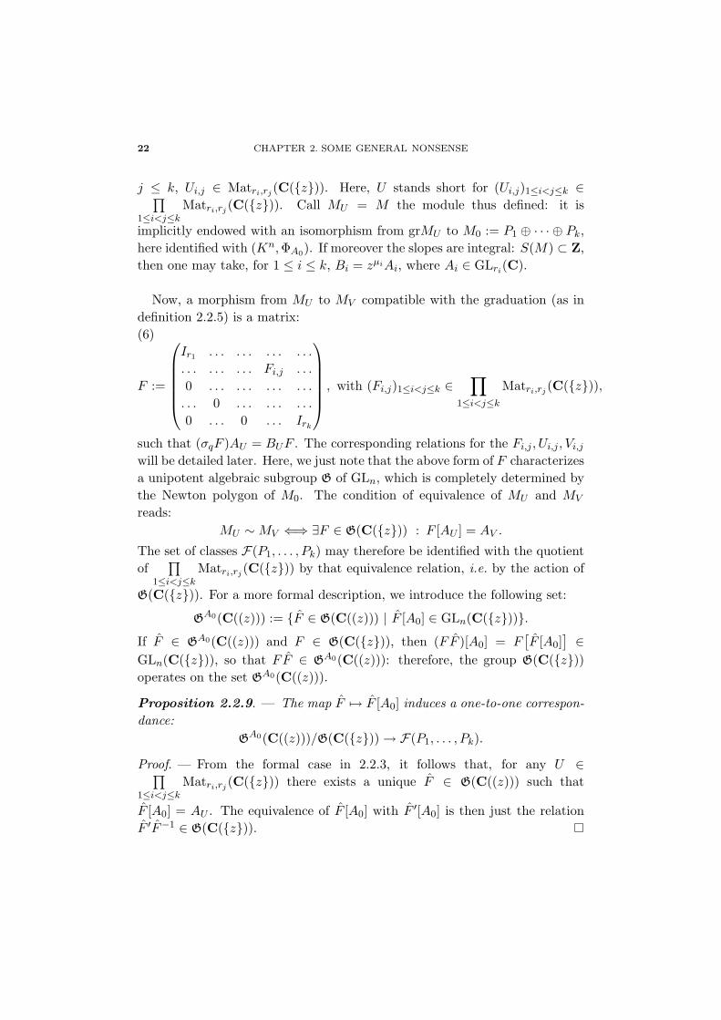
Now, a morphism from MU to MV compatible with the graduation (as indefinition 2.2.5) is a matrix:(6)
F :=
Ir1 . . . . . . . . . . . .
. . . . . . . . . Fi,j . . .
0 . . . . . . . . . . . .
. . . 0 . . . . . . . . .
0 . . . 0 . . . Irk
, with (Fi,j)1≤i<j≤k ∈∏
1≤i<j≤k
Matri,rj (C(z)),
such that (σqF )AU = BUF . The corresponding relations for the Fi,j , Ui,j , Vi,j
will be detailed later. Here, we just note that the above form of F characterizesa unipotent algebraic subgroup G of GLn, which is completely determined bythe Newton polygon of M0. The condition of equivalence of MU and MV
reads:MU ∼MV ⇐⇒ ∃F ∈ G(C(z)) : F [AU ] = AV .
The set of classes F(P1, . . . , Pk) may therefore be identified with the quotientof
∏1≤i<j≤k
Matri,rj (C(z)) by that equivalence relation, i.e. by the action of
G(C(z)). For a more formal description, we introduce the following set:
GA0(C((z))) := F ∈ G(C((z))) | F [A0] ∈ GLn(C(z)).
If F ∈ GA0(C((z))) and F ∈ G(C(z)), then (FF )[A0] = F[F [A0]
]∈
GLn(C(z)), so that FF ∈ GA0(C((z))): therefore, the group G(C(z))operates on the set GA0(C((z))).
Proposition 2.2.9. — The map F 7→ F [A0] induces a one-to-one correspon-dance:
GA0(C((z)))/G(C(z))→ F(P1, . . . , Pk).
Proof. — From the formal case in 2.2.3, it follows that, for any U ∈∏1≤i<j≤k
Matri,rj (C(z)) there exists a unique F ∈ G(C((z))) such that
F [A0] = AU . The equivalence of F [A0] with F ′[A0] is then just the relationF ′F−1 ∈ G(C(z)).
2.3. CLASSIFICATION OF ISOGRADED FILTERED DIFFERENCE MODULES 23
Remark 2.2.10. — Write FU for the F in the above proof. More generally,for any U, V ∈
∏1≤i<j≤k
Matri,rj (C(z)) there exists a unique F ∈ G(C((z)))
such that F [AU ] = AV ; write it FU,V . Then FU,V = FV F−1U and the condition
of equivalence of MU and MV reads:
MU ∼MV ⇐⇒ FU,V ∈ G(C(z)).
Giving analyticity conditions for a formal object strongly hints towards aresummation problem! (See chapters 4 and 5.)
2.3. Classification of isograded filtered difference modules
2.3.1. General setting of the problem. — Definition 2.2.5 obviouslyadmits a purely algebraic generalization, which is related to some interestingproblems in homological algebra. We shall now describe in some detail resultsin that direction, from [23]; this will give us an adequate frame to formulateand prove our first structure theorem for the space of isoformal analytic classes.
Let C a commutative ring and C an abelian C-linear category. We fix afinitely graded object:
P = P1 ⊕ · · · ⊕ Pk,
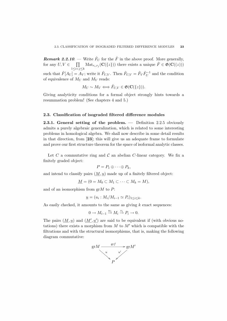
and intend to classify pairs (M,u) made up of a finitely filtered object:
M = (0 = M0 ⊂M1 ⊂ · · · ⊂Mk = M),
and of an isomorphism from grM to P :
u = (ui : Mi/Mi−1 ' Pi)1≤i≤k.
As easily checked, it amounts to the same as giving k exact sequences:
0→Mi−1wi→Mi
vi→ Pi → 0.
The pairs (M,u) and (M ′, u′) are said to be equivalent if (with obvious no-tations) there exists a morphism from M to M ′ which is compatible with thefiltrations and with the structural isomorphisms, that is, making the followingdiagram commutative:
grMu
!!CCCC
CCCC
grf // grM ′
u′
||zzzz
zzzz
P
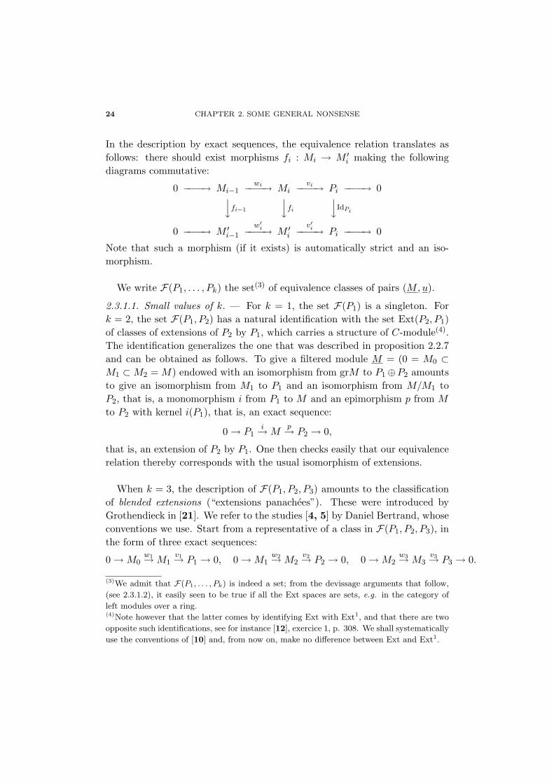
24 CHAPTER 2. SOME GENERAL NONSENSE
In the description by exact sequences, the equivalence relation translates asfollows: there should exist morphisms fi : Mi → M ′
i making the followingdiagrams commutative:
0 −−−−→ Mi−1wi−−−−→ Mi
vi−−−−→ Pi −−−−→ 0yfi−1
yfi
yIdPi
0 −−−−→ M ′i−1
w′i−−−−→ M ′i
v′i−−−−→ Pi −−−−→ 0
Note that such a morphism (if it exists) is automatically strict and an iso-morphism.
We write F(P1, . . . , Pk) the set(3) of equivalence classes of pairs (M,u).
2.3.1.1. Small values of k. — For k = 1, the set F(P1) is a singleton. Fork = 2, the set F(P1, P2) has a natural identification with the set Ext(P2, P1)of classes of extensions of P2 by P1, which carries a structure of C-module(4).The identification generalizes the one that was described in proposition 2.2.7and can be obtained as follows. To give a filtered module M = (0 = M0 ⊂M1 ⊂M2 = M) endowed with an isomorphism from grM to P1⊕P2 amountsto give an isomorphism from M1 to P1 and an isomorphism from M/M1 toP2, that is, a monomorphism i from P1 to M and an epimorphism p from M
to P2 with kernel i(P1), that is, an exact sequence:
0→ P1i→M
p→ P2 → 0,
that is, an extension of P2 by P1. One then checks easily that our equivalencerelation thereby corresponds with the usual isomorphism of extensions.
When k = 3, the description of F(P1, P2, P3) amounts to the classificationof blended extensions (“extensions panachees”). These were introduced byGrothendieck in [21]. We refer to the studies [4, 5] by Daniel Bertrand, whoseconventions we use. Start from a representative of a class in F(P1, P2, P3), inthe form of three exact sequences:
0→M0w1→M1
v1→ P1 → 0, 0→M1w2→M2
v2→ P2 → 0, 0→M2w3→M3
v3→ P3 → 0.
(3)We admit that F(P1, . . . , Pk) is indeed a set; from the devissage arguments that follow,
(see 2.3.1.2), it easily seen to be true if all the Ext spaces are sets, e.g. in the category of
left modules over a ring.(4)Note however that the latter comes by identifying Ext with Ext1, and that there are two
opposite such identifications, see for instance [12], exercice 1, p. 308. We shall systematically
use the conventions of [10] and, from now on, make no difference between Ext and Ext1.
2.3. CLASSIFICATION OF ISOGRADED FILTERED DIFFERENCE MODULES 25
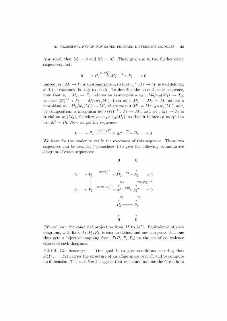
Also recall that M0 = 0 and M3 = M . These give rise to two further exactsequences; first:
0 // P1
w2v−11 // M2
v2 // P2// 0
Indeed, v1 : M1 → P1 is an isomorphism, so that v−11 : P1 →M1 is well defined;
and the exactness is easy to check. To describe the second exact sequence,note that v2 : M2 → P2 induces an isomorphism v2 : M2/w2(M1) → P2,whence (v2)−1 : P2 → M2/w2(M1); then w3 : M2 → M3 = M induces amorphism w3 : M2/w2(M1)→M ′, where we put M ′ := M/w3 w2(M1), and,by composition, a morphism w3 (v2)−1 : P2 → M ′; last, v3 : M3 → P3 istrivial on w3(M2), therefore on w3 w2(M1), so that it induces a morphismv3 : M ′ → P3. Now we get the sequence:
0 // P2w3(v2)−1
// M ′ v3 // P3// 0
We leave for the reader to verify the exactness of this sequence. These twosequences can be blended (“panachees”) to give the following commutativediagram of exact sequences:
0
0
0 // P1
w2v−11 // M2
v2 //
w3
P2//
w3(v2)−1
0
0 // P1
w3w2v−11 // M
can //
v3
M ′ //
v3
0
P3
P3
0 0
(We call can the canonical projection from M to M ′.) Equivalence of suchdiagrams, with fixed P1, P2, P3, is easy to define, and one can prove that onethus gets a bijective mapping from F(P1, P2, P3) to the set of equivalenceclasses of such diagrams.
2.3.1.2. The devissage. — Our goal is to give conditions ensuring thatF(P1, . . . , Pk) carries the structure of an affine space over C, and to computeits dimension. The case k = 2 suggests that we should assume the C-modules
26 CHAPTER 2. SOME GENERAL NONSENSE
Ext(Pj , Pi) to be free of finite rank. (As we shall see, the only pairs thatmatter are those with i < j.) Then, aiming at an induction argument, oneinvokes a natural onto mapping:
F(P1, . . . , Pk) −→ F(P1, . . . , Pk−1),
sending the class of (M,u) defined as above to the class of (M ′, u′) defined by:
M ′ = (0 = M0 ⊂M1 ⊂ · · · ⊂Mk−1 = M ′) et u′ = (ui)1≤i≤k−1.
The preimage of the class of (M ′, u′) described above is identified withExt(Pk,M
′); and note that Ext(Pk,M′) indeed only depends (up to a canon-
ical isomorphism) on the class of (M ′, u′). Under the assumptions we shallchoose, we shall see that Ext(Pk,M
′) can in turn be unscrewed (devisse)in the Ext(Pk, Pi) for i < k, and we expect to get a space with dimension∑1≤i<j≤k
dim Ext(Pj , Pi).
Remark 2.3.1. — Once described the space F(P1, . . . , Pk), one can ask forthe seemingly more natural problem of the classification of those objects Msuch that grM ' P (without prescrit of the “polarization” u). One checks thatthe group
∏Aut(Pi) operates on the space F(P1, . . . , Pk): actually, (φi) ∈∏
Aut(Pi) acts on the “class” of all pairs (M,u) through left compositionsφi ui. Then, our new classification comes by quotienting F(P1, . . . , Pk) bythis action. We shall not deal with that problem.
The use of homological algebra in classification problems for functionalequations is ancient, but it seems that the first step, the algebraic modeli-sation, has sometimes been tackled rather casually: for instance, when identi-fying a module of extensions with a cokernel, the explicit description of a mapis almost always given; the proof of its bijectivity comes sometimes; the proofof its additivity seldom; the proof of its linearity (seemingly) never. For thatreason, very great care has been given here to detailed algebraic constructionsand proofs of “obvious” isomorphisms.
2.3.2. Difference modules over difference rings. — In order to studya relative situation from 2.3.4 on, we now generalize to difference rings ourbasic constructions. Let K be a commutative ring and σ a ring automorphismof K. As noticed in 2.1.1, most constructions and statements about differencefields and modules remain valid over the difference ring (K,σ). Now let C bea commutative ring (we may think of the the field C of complex numbers, orelse some arbitrary field of “constants”). Assume that K is a commutative
2.3. CLASSIFICATION OF ISOGRADED FILTERED DIFFERENCE MODULES 27
C-algebra and σ a C-algebra automorphism, that is, a C-linear ring automor-phism. Then the ring of constants Kσ := x ∈ K | σx = x is actually a subC-algebra of K, and the Ore ring of difference operators DK,σ := K < σ, σ−1 >
is a C-algebra with center Kσ. (As before, its elements are non-commutativeLaurent polynomials with the twisted commutation relations σk.λ = σk(λ)σk).
A difference module over the difference C-algebra (K,σ) (more shortly, overK) will be defined to be a left DK,σ-module which, by restriction of scalars toK, yields a finite rank projective K-module. We write DiffMod(K,σ) thefull subcategory of DK,σ −Mod with objects the difference modules over K.Both categories are abelian and C-linear. Left DK,σ-modules (resp. differencemodules over K) can be realized as pairs (E,Φ), where E is a K-module (resp.projective of finite rank) and Φ is a semi-linear automorphism of E, that is,a group automorphism such that ∀λ ∈ K , ∀x ∈ E , Φ(λx) = σ(λ)Φ(x). Inthis description, a morphism of DK,σ-modules from (E,Φ) to (F,Ψ) is a mapu ∈ LK(E,F ) such that Ψ u = u Φ.
2.3.2.1. Matricial description of difference modules. — Here, we assume thatthe K-module E is free of finite rank n. This assumption will be maintainedin 2.3.2.2 and 2.3.3.2, where we pursue the matricial description. Choosing abasis B allows one to identify E with Kn. It is then clear that Φ(B) is also abasis of E, whence the existence of A ∈ GLn(K) such that Φ(B) = BA−1. Ifx ∈ E has the coordinate column vector X ∈ Kn in basis B, i.e. if x = BX,computing Φ(x) = Φ(BX) = Φ(B)σ(X) = BA−1σ(X) shows that Φ(x) ∈ Ehas the coordinate column vector A−1σ(X); we thus may identify (E,Φ) '(Kn,ΦA), where ΦA(X) := A−1σ(X). Morphisms from (Kn,ΦA) to (Kp,ΦB)are matrices F ∈Mp,n(K) such that (σF )A = BF and their composition boilsdown to matrix product. In particular, isomorphism of modules is describedby gauge transformations:
(Kn,ΦA) ' (Kp,ΦB)⇐⇒ n = p et ∃F ∈ GLn(K) : B = F [A] := (σF )AF−1.
2.3.2.2. Matricial description of filtered difference modules. — Let Pi =(Gi,Ψi) (1 ≤ i ≤ k) be difference modules such that each K-module Gi is freeof finite rank ri . For each Gi, choose a basis Di, and write Bi ∈ GLri(K) theinvertible matrix such that Ψi(Di) = DiBi.
Let M be a finitely filtered difference module with associated graded moduleP = P1 ⊕ · · · ⊕ Pk; more precisely, M = (0 = M0 ⊂ M1 ⊂ · · · ⊂ Mk = M) isequipped with an isomorphism u = (ui : Mi/Mi−1 ' Pi)1≤i≤k from grM to P .
28 CHAPTER 2. SOME GENERAL NONSENSE
Letting Mi = (Ei,Φi), one builds a basis Bi of Ei by induction on i = 1, . . . , kin such a way that Bi−1 ⊂ Bi and that B′i := Bi \ Bi−1 lifts Di via ui (showingby the way that K-modules Ei are free of finite ranks r1 + · · · + ri). WriteΦi (resp. Φi) the semi-linear automorphism induced by Φ (resp. by Φi) onEi (resp. on Ei/Ei−1), and Ci the basis of Ei/Ei−1 induced by B′i, one drawsfrom equality ui Φi = Ψi ui (due to the fact that ui is a morphism) therelation: Φi(Ci) = CiBi, then, from the latter, the relation:
Φi(B′i) ≡ B′iBi (mod Ei−1).
Last, one gets that the matrix of Φ in basis B is block upper-triangular:
Φ(B) = B
B1 ? ?
0. . . ?
0 0 Bk
.
As in 2.3.2.1, we identify Pi (1 ≤ i ≤ k) with (Kri ,ΦAi), where Ai := B−1i ∈
GLri(K). Likewise, P is identified with (Kn,ΦA0) and M with (Kn,ΦA),where n := r1 + · · ·+ rk and:
A0 =
A1 0 0
0. . . 0
0 0 Ak
et A =
A1 ? ?
0. . . ?
0 0 Ak
.
Note that these relations implicitly presuppose that a filtration on M is given,as well as an isomorphism from grM to P . If moreover M ′ = (Kn,ΦA′),where A′ has the same form as A (i.e. M ′ is filtered and equipped with anisomorphism from grM ′ to P ), then, a morphism from M to M ′ respectingfiltrations (i.e. sending each Mi into M ′
i) is described by a matrix F in thefollowing block upper triangular form; and the induced endomorphism of P 'grM ' grM ′ is described by the corresponding block diagonal matrix F0
F =
F1 ? ?
0. . . ?
0 0 Fk
et F0 =
F1 0 0
0. . . 0
0 0 Fk
.
In particular, a morphism inducing identity on P (thus ensuring that the fil-tered modules M,M ′ belong to the same class in F(P1, . . . , Pk)) is represented

2.3. CLASSIFICATION OF ISOGRADED FILTERED DIFFERENCE MODULES 29
by a matrix in G(K), where we denote G the algebraic subgroup of GLn de-fined by the following shape: Ir1 ? ?
0. . . ?
0 0 Irk
.
Now write AU the block upper triangular matrix with block diagonal compo-nent A0 and with upper triangular blocks the Ui,j ∈Mri,rj (K) (1 ≤ i < j ≤ k);here, U is an abrevation for the family (Ui,j). For all F ∈ G(K), the matrixF [AU ] is equal to AV for some family of Vi,j ∈ Mri,rj (K). Thus, the groupG(K) operates on the set
∏1≤i<j≤k
Mri,rj (K). The above discussion can be
summarised as follows:
Proposition 2.3.2. — The map sending U to the class of (Kn,ΦAU) induces
a bijection from the quotient of the set∏
1≤i<j≤k
Mri,rj (K) under the action of
the group G(K) onto the set F(P1, . . . , Pk).
2.3.3. Extensions of difference modules. — Let 0 → M ′ → M →M ′′ → 0 an exact sequence in DK,σ − Mod. If M ′,M ′′ are differencemodules, so is M (it is projective of finite rank because we have a splitsequence of K-modules). The calculus of extensions is therefore the same inDiffMod(K,σ) as in DK,σ −Mod and we will simply write Ext(M ′′,M ′) thegroup ExtDK,σ
(M ′′,M ′) of classes of extensions of M ′′ by M ′. According to[10, §7], this group is actually endowed with a structure of C-module, whichis well described in loc. cit.(5). We shall now make explicit that structure inthe case that M ′ and M ′′ are difference modules.
So let M = (E,Φ) and N = (F,Ψ). Any extension 0→ N → R→ M → 0of M by N gives rise (by restriction of scalars) to an exact sequence of K-modules 0→ F → G→ E → 0 such that, if R = (G,Γ), the following diagramis commutative:
0 −−−−→ Fi−−−−→ G
j−−−−→ E −−−−→ 0yΨ
yΓ
yΦ
0 −−−−→ Fi−−−−→ G
j−−−−→ E −−−−→ 0
(5)And, to the best of our knowledge, nowhere else.
30 CHAPTER 2. SOME GENERAL NONSENSE
(We wrote again i, j the underlying K-linear maps.) Since E is projective, thesequence is split and one can from start identify G with the K-module F ×E,thus writing i(y) = (y, 0) and j(y, x) = x. The compatibility conditionsΓ i = i Ψ and Φ j = j Γ then imply:
Γ(y, x) = Γu(y, x) :=(Ψ(y) + u(x),Φ(x)
), with u ∈ Lσ(E,F ),
where we write Lσ(E,F ) the set of σ-linear maps from E to F . (This meansthat u is a group morphism such that u(λx) = σ(λ)u(x).) Setting moreoverRu := (F × E,Γu), which is a difference module naturally equipped with astructure of extension of M by N , we see that we have defined a surjectivemap:
Lσ(E,F )→ Ext(M,N),
u 7→ θu := class of Ru.
We can make precise the conditions under which u, v ∈ Lσ(E,F ) have thesame image θu = θv, i.e. under which Ru and Rv are equivalent extensions.This happens if there exists a morphism φ : Ru → Rv inducing the identitymap on M and N , that is, a linear map φ : F × E → F × E such thatΓv φ = φ Γu (since it is a morphism of difference modules) and having theform (x, y) 7→
(y + f(x), x
)(since it induces the identity maps on E and on
F ). Now, the first condition becomes:
∀(y, x) ∈ F ×E ,(Ψ(y+f(x))+v(x),Φ(x)
)=(Ψ(y)+u(x)+f(Φ(x)),Φ(x)
),
that is:
u− v = Ψ f − f Φ.
Remark by the way that, for all f ∈ LK(E,F ), the map tΦ,Ψ(f) := Ψf−f Φis σ-linear from E to F .
Theorem 2.3.3. — The map u 7→ θu from Lσ(E,F ) to Ext(M,N) is func-torial in M and in N , C-linear, and its kernel is the image of the C-linearmap:
tΦ,Ψ : LK(E,F )→ Lσ(E,F ),
f 7→ Ψ f − f Φ.
Proof. — Functoriality.We shall only prove (and use) it on the covariant side, i.e. in N . We invoke[10, §7.1 p. 114, example 3 and §7.4, p. 119, prop. 4]. Let θ be the class

2.3. CLASSIFICATION OF ISOGRADED FILTERED DIFFERENCE MODULES 31
in Ext(M,N) of the extension 0 i→ N → Rj→ M → 0 and g : N → N ′ a
morphism in DiffMod(K,σ). Let
0 −−−−→ Ni−−−−→ R
j−−−−→ M −−−−→ 0yg
yh
yIdM
0 −−−−→ N ′ i′−−−−→ R′j′−−−−→ M −−−−→ 0
be a commutative diagram of exact sequences. If θ′ is the class in Ext(M,N)
of the extension 0 i′→ N ′ → R′j′→M → 0, then:
Ext(IdM , g)(θ) = g θ = θ′ IdM = θ′.
We take:
R′ := R⊕N N ′ =R×N ′
(i(n),−g(n)
)| n ∈ N
,
with i′, j′ the obvious arrows, and for R the extension Ru; with the previousnotations for N,M,R, and also writing N ′ = (F ′,Ψ′), with compatibilitycondition Ψ′ g = g Ψ, we see that the K-module underlying R⊕N N ′ is:
G′ :=F × E × F ′
(y, 0,−g(y)
)| y ∈ F
,
endowed with the semi-linear automorphism induced by the map Γu×Ψ′ fromF × E × F ′ to itself (the latter does fix the denominator).The map (y, x, y′) 7→
(y′ + g(y), x
)from F × E × F ′ to F ′ × E induces an
isomorphism from G′ to F ′ × E and the induced semi-linear automorphismon G′ is (y′, x) 7→
(Ψ′(y′) + g
(u(x)
),Φ(x)
), that is Γgu, from which it follows
that R′ = Rgu. The arrows i′, j′ are determined as follows: i′(y′) is theclass of (0, y′) in G′, that is, under the previous identification, i′(y′) = (y′, 0);and j′(y′, x) is the image of an arbitrary preimage, for instance the class of(0, x, y′): that image is j(0, x) = x. We have therefore shown that the class ofthe extension Ru by Ext(IdM , g) is Rgu, which is the wanted functoriality. Itis expressed by the commutativity of the following diagram:
Lσ(E,F ) −−−−→ Ext(M,N)yLσ(IdM ,g)
yExt(IdM ,g)
Lσ(E,F ′) −−−−→ Ext(M,N ′)Linearity.According to the remark just before the theorem, the map tΦ,Ψ indeed sendsLK(E,F ) to Lσ(E,F ).Addition. The reference here is [10, §7.6, rem. 2 p. 124]. From the extensions

32 CHAPTER 2. SOME GENERAL NONSENSE
0 → Ni→ R
p→ M → 0 and 0 → Ni′→ R′
p′→ M → 0 having classesθ, θ′ ∈ Ext1(M,N), one computes θ + θ′ as the class of the extension 0 →N
i′′→ R′′p′′→M → 0, where:
R′′ :=(z, z′) ∈ R×R′ | p(z) = p′(z′)(−i(y), i′(y)) | y ∈ N
,
and i′′(y) is the class of (0, i′(y)), i.e. the same as the class of (i(y), 0); and p′′
sends the class of (z, z′) to p(z) = p′(z′). Taking R = Ru and R′ = Ru′ , thenumerator of R′′ is identified with F × F × E equipped with the semi-linearautomorphism (y, y′, x) 7→ (Ψ(y)+u(x),Ψ(y′)+u′(x),Φ(x)). The denominatoris identified with the subspace (−y, y, 0) | y ∈ F equipped with the inducedmap. The quotient is identified with 0× F ×E, through the map (y, y′, x) 7→(0, y′′, x), where y′′ := y′ + y, equipped with the semi-linear automorphism Φ′′
which sends (0, y′′, x) to
(0,Ψ(y′) + u′(x) + Ψ(y) + u(x),Φ(x)) = (0,Ψ(y′′) + (u+ u′)(x),Φ(x)).
This is indeed Ru+u′ .External multiplication. The reference here is [10, §7.6, prop. 4 p. 119].Let λ ∈ C. We apply the invoked proposition to the following commutativediagram of exact sequences:
0 −−−−→ N −−−−→ Ru −−−−→ M −−−−→ 0y×λ
y(×λ,IdM )
yIdM
0 −−−−→ N −−−−→ Rλu −−−−→ M −−−−→ 0
If θ, θ′ are the classes in Ext(M,N) of the two extensions, one infers from loc.cit. that:
θ′ IdM = (×λ) θ =⇒ θ′ = λθ.
The class of the extension Rλu is therefore indeed equal to the product of λby the class of the extension Ru.
Exactness.It follows immediately from the computation shown just before the statementof the theorem.
2.3.3.1. The complex of solutions. — The following is sometimes consideredas a difference analog of the de Rham complex in one variable, see for instance[1, 49].

2.3. CLASSIFICATION OF ISOGRADED FILTERED DIFFERENCE MODULES 33
Definition 2.3.4. — We call complex of solutions of M in N the followingcomplex of C-modules:
tΦ,Ψ : LK(E,F )→ Lσ(E,F ),
f 7→ Ψ f − f Φ.
concentrated in degrees 0 and 1.
It is indeed clear that the source and target are C-modules, that the maptΦ,Ψ does sends the source into the target and that it is C-linear.
Corollary 2.3.5. — The homology of the complex of solutions is H0 =Hom(M,N) and H1 = Ext(M,N), and these equalities are functorial.
Proof. — The statement about H1 is the theorem. As regards H0, the kernelof tΦ,Ψ is the C-module f ∈ LK(E,F ) | Ψ f = f Φ, that is, Hom(M,N);and functoriality is obvious in that case.
Corollary 2.3.6. — From the exact sequence 0→ N ′ → N → N ′′ → 0, onededuces the “cohomology long exact sequence”:
0→ Hom(M,N ′)→Hom(M,N)→ Hom(M,N ′′)
→ Ext(M,N ′)→ Ext(M,N)→ Ext(M,N ′′)→ 0.
Proof. — We keep the previous notations (and moreover adapt them toN ′, N ′′). The exact sequence of projective K-modules 0→ F ′ → F → F ′′ → 0being split, both lines of the commutative diagram:
0 −−−−→ LK(E,F ′) −−−−→ LK(E,F ) −−−−→ LK(E,F ′′) −−−−→ 0ytΦ,Ψ′
ytΦ,Ψ
ytΦ,Ψ′′
0 −−−−→ Lσ(E,F ′) −−−−→ Lσ(E,F ) −−−−→ Lσ(E,F ′′) −−−−→ 0
are exact, and it is enough to call to the snake lemma.
2.3.3.2. Matricial description of extensions of difference modules. — Wenow assume E,F to be free of finite rank over K and accordingly identifythem with M = (Km,ΦA), A ∈ GLm(K) and N = (Kn,ΦB), B ∈ GLn(K).An extension of N by M then takes the form R = (Km+n,ΦC), where
C =(
A U
0n,m B
)for some rectangular matrix U ∈ Mm,n(K); we shall write
C = CU . The injection M → R and the projection R→ N have as respective
matrices(Im
0n,m
)and
(0n,m In
). The extension thus defined will be denoted

34 CHAPTER 2. SOME GENERAL NONSENSE
RU .
A morphism of extensions RU → RV is a matrix of the form F =(Im X
0n,m In
)for some rectangular matrix X ∈ Mm,n(K). The compatibility
condition with the semi-linear automorphisms writes:
(σF )CU = CV F ⇐⇒ U + (σX)B = AX + V ⇐⇒ V − U = (σX)B −AX.
Corollary 2.3.7. — The C-module Ext1(N,M) is thereby identified with thecokernel of the endomorphism X 7→ (σX)B −AX of Mm,n(K).
Proof. — The above construction provides us with a bijection, but it followsfrom theorem 2.3.3 that it is indeed an isomorphism.
2.3.4. Extension of scalars. — We want to see F(P1, . . . , Pk) as a schemeover C, that is as a representable functor C ′ ; F(C ′ ⊗C P1, . . . , C
′ ⊗C Pk)from commutative C-algebras to sets. To that end, we shall extend what wedid to a “relative” situation.
Let C ′ be a commutative C-algebra. We set:
K ′ := C ′ ⊗C K and σ′ := 1⊗C σ.
Then K ′ is a commutative C ′-algebra and σ′ an automorphism of that C ′-algebra. Moreover:
DK′,σ′ := K ′ < σ′, σ′−1
>= K ′ ⊗K DK,σ = C ′ ⊗C DK,σ.
These equalities should be interpreted as natural (functorial) isomorphisms.
From any difference module M = (E,Φ) over (K,σ), one gets a differencemodule M ′ = (E′,Φ′) over (K ′, σ′) by putting:
E′ = K ′ ⊗K E = C ′ ⊗C E and Φ′ = σ′ ⊗K Φ = 1⊗C Φ.
(This is indeed a left DK′,σ′-module and it is projective of finite rank over K ′.)We shall write it M ′ = C ′ ⊗k M to emphasize the dependency on C ′. Thefollowing proposition is the tool to tackle the case k = 2.
Proposition 2.3.8. — Let M,N be two difference modules over (K,σ). Onehas a functorial isomorphism of C ′-modules:
ExtDK′,σ′ (C′ ⊗C M,C ′ ⊗C N) ' C ′ ⊗C ExtDK,σ
(M,N),

2.3. CLASSIFICATION OF ISOGRADED FILTERED DIFFERENCE MODULES 35
and a functorial epimorphism of C ′-modules:
C ′ ⊗C HomDK,σ(M,N)→ HomDK′,σ′ (C
′ ⊗C M,C ′ ⊗C N).
Proof. — We shall write M ′ = C ′ ⊗C M , E′ = K ′ ⊗K E etc. The K-modulesE,F beeing projective of finite rank, there are natural isomorphisms:
C ′ ⊗C LK(E,F ) = LK′(E′, F ′) et C ′ ⊗C Lσ(E,F ) = Lσ′(E′, F ′).
(This is immediate if E and F are free, the general case follows.) By tensoringthe (functorial) exact sequence:
0→ HomDK,σ(M,N)→ LK(E,F )→ Lσ(E,F )→ ExtDK,σ
(M,N)→ 0,
we get the exact sequence:
C ′⊗CHomDK,σ(M,N)→ C ′⊗CLK(E,F )→ C ′⊗CLσ(E,F )→ C ′⊗CExtDK,σ
(M,N)→ 0.
Both conclusions then come by comparison with the exact sequence:
0→ HomDK′,σ′ (M′, N ′)→ LK′(E′, F ′)→ Lσ′(E′, F ′)→ ExtDK′,σ′ (M
′, N ′)→ 0.
Proposition 2.3.9. — Let 0 = M0 ⊂ M1 ⊂ · · · ⊂ Mk = M be a k-filtrationwith associated graded module P1 ⊕ · · · ⊕ Pk. Then, setting M ′
i := C ′ ⊗C Mi
and P ′i := C ′⊗C Pi, we get a k-filtration 0 = M ′0 ⊂M ′
1 ⊂ · · · ⊂M ′k = M ′ with
associated graded module P ′1 ⊕ · · · ⊕ P ′k.
Proof. — The Pi being projective as K-modules, the exact sequences 0 →Mi−1 →Mi → Pi → 0 are K-split, so they give rise by the base change K ′⊗K
to exact sequences 0→M ′i−1 →M ′
i → P ′i → 0.
If (M,u) denotes the pair made up of the above k-filtered object and of afixed isomorphism from grM to P1⊕· · ·⊕Pk, we shall write (C ′⊗CM, 1⊗C u)the corresponding pair deduced from the proposition.
Definition 2.3.10. — We define as follows a functor F from the categoryof commutative C-algebras to the category of sets. For any commutative C-algebra C ′, we set:
F (C ′) := F(C ′ ⊗C P1, . . . , C′ ⊗C Pk).
For any morphism C ′ → C ′′ of commutative C-algebras, the map F (C ′) →F (C ′′) is given by:
class of (M ′, u′) 7→ class of (C ′′ ⊗k′ M′, 1⊗C u
′).
36 CHAPTER 2. SOME GENERAL NONSENSE
The set F (C ′) is well defined according to the previous constructions. Themap F (C ′) → F (C ′′) is well defined on pairs thanks to the proposition, andthe reader will check that it goes to the quotient. Last, the functoriality(preservation of the composition of morphisms) comes from the contractionrule of tensor products:
C ′′′ ⊗C′′ (C ′′ ⊗C′ M ′) = C ′′′ ⊗C′ M ′.
2.3.5. Our moduli space. — To simplify, herebelow, instead of saying “thefunctor F is represented by an affine space over C (with dimension d)”, weshall say “the functor F is an affine space over C (with dimension d)”. Thisis just the usual identification of a scheme with the space it represents.
Theorem 2.3.11. — Assume that, for 1 ≤ i < j ≤ k, one has Hom(Pj , Pi) =0 and that the C-module Ext(Pj , Pi) is free of finite rank δi,j. Then the functorC ′ ; F (C ′) := F(C ′ ⊗C P1, . . . , C
′ ⊗C Pk) is an affine space over C withdimension
∑1≤i<j≤k
δi,j.
Proof. — When k = 1, it is trivial. When k = 2, writing V the free C-moduleof finite rank Ext(P2, P1), and appealing to proposition 2.3.8, we see that thisis the functor C ′ ; C ′ ⊗C V , which is represented by the symetric algebraof the dual of V , an algebra of polynomials over C. For k ≥ 3, we use aninduction based on a lemma of Babbitt and Varadarajan [2, lemma 2.5.3, p.139]:
Lemma 2.3.12. — Let u : F → G be a natural transformation between twofunctors from commutative C-algebras to sets. Assume that G is an affinespace over C and that, for any commutative C-algebra C ′, and for any b ∈G(C ′), the following functor “fiber above b” from commutative C ′-algebras tosets:
C ′′ ; u−1C′′(G(C ′ → C ′′)(b)
)is an affine space over C ′. Then F is an affine space over C.
In loc. cit., this theorem is proved for C = C, but the argument isplainly valid for any commutative ring. Here is its skeleton. Choose B =C[T1, . . . , Td] representing G. Take for b the identity of G(B) = Hom(B,B)(“general point”); the fiber is represented by B[S1, . . . , Se]. One then showsthat C[T1, . . . , Td, S1, . . . , Se] represents F . This gives by the way a computa-tion of dimF as dimG + dim of the general fiber. In our case, all fibers willhave the same dimension.
2.3. CLASSIFICATION OF ISOGRADED FILTERED DIFFERENCE MODULES 37
2.3.5.1. Structure of the fibers. — Before going to the proof of the theorem,we need an auxiliary result.
Proposition 2.3.13. — Let C ′ be a commutative C-algebra and let M ′ bea difference module over K ′ := C ′ ⊗C K, equipped with a (k − 1)-filtration:0 = M ′
0 ⊂ M ′1 ⊂ · · · ⊂ M ′
k−1 = M ′ such that grM ′ ' P ′1 ⊕ · · · ⊕ P ′k−1
(as usual, P ′i := C ′ ⊗C Pi). Then the functor in commutative C ′-algebrasC ′′ ; Ext(C ′′ ⊗C Pk, C
′′ ⊗C′ M ′) is an affine space over C ′ with dimension∑1≤i≤k
δi,k.
Proof. — After proposition 2.3.8, this is the functor C ′′ ; C ′′⊗C′Ext(P ′k,M′).
From each exact sequence 0 → M ′i−1 → M ′
i → P ′i → 0 one draws the coho-mology long exact sequence of corollary 2.3.6; but, from proposition 2.3.8, onedraws that, for any commutative C-algebra C ′, one has Hom(C ′⊗C Pj , C
′⊗C
Pi) = 0 and that the C ′-module Ext(C ′ ⊗C Pj , C′ ⊗C Pi) is free of finite rank
δi,j . According to the equalities Hom(P ′j , P′i ) = 0, the long exact sequence is
here shortened as:
0→ Ext(P ′k,M′i−1)→ Ext(P ′k,M
′i)→ Ext(P ′k, P
′i )→ 0,
and, for i = 1, . . . , k− 1, these sequences are split, the term at the right beingfree. So, in the end:
Ext(P ′k,M′) '
⊕1≤i≤k
Ext(P ′k, P′i ),
which is free of rank∑
1≤i≤k
δi,k. As in the case k = 2 (which is a particular
case of the proposition), the functor mentioned is represented by the symetricalgebra of the dual of this module.
For all ` such that 1 ≤ ` ≤ k, let us write:
V` :=⊕
1≤i≤`
Ext(P`, Pi),
W` :=⊕
1≤i<j≤`
Ext(Pj , Pi),
V ′` :=⊕
1≤i≤`
Ext(P ′`, P′i ),
W ′` :=
⊕1≤i<j≤`
Ext(P ′j , P′i ).

38 CHAPTER 2. SOME GENERAL NONSENSE
We consider V`,W` as affine schemes over C and V ′` ,W′` as affine schemes over
C ′, so that:
V ′` = C ′ ⊗C V`, W ′` = C ′ ⊗C W`.
We improperly write C ′⊗CV the base change of affine schemes Spec C ′⊗Spec C
V . Also, we do not distinguish between the direct sums of the free C-modulesExt(Pj , Pi) and the product of the corresponding affine schemes. Note that, inthe proof of the proposition, the isomorphism Ext(P ′k,M
′) ' V ′` is functorialin C ′. This entails:
Corollary 2.3.14. — Each fiber Ext(P ′k,M′) is isomorphic to V ′k as a
scheme over C ′.
2.3.5.2. End of the proof of theorem 2.3.11. — Now we end the proof of thetheorem. Besides functor F (C ′), we consider the functor C ′ ; G(C ′) :=F(C ′ ⊗C P1, . . . , C
′ ⊗C Pk−1), of which we assume, by induction, that it is anaffine space of dimension
∑1≤i<j≤k−1
δi,j . The natural transformation from F
to G is the one described in 2.3.1.2. An element b ∈ G(C ′) is the class of apair (M ′, u′), a (k − 1)-filtered object over C ′, and the corresponding fiber isthe one studied in the above auxiliary proposition 2.3.13. The lemma 2.3.12of Babbitt and Varadarajan then allows us to conclude.
Looking at the proof of 2.3.12, one moreover sees that, if all fibers of u :F → G are isomorphic to a same affine space V (up to obvious extension ofthe base), then there is an isomorphism F ' V ×C G such that u correspondsto the second projection. With the previous notations, we see that, writingF` the functor C ′ ; F(C ′ ⊗C P1, . . . , C
′ ⊗C P`), corollary 2.3.13 gives anisomorphism of schemes:
F` ' F`−1 × V`.
By induction, we conclude:
Corollary 2.3.15. — The functor in C-algebras C ′ ; F(C ′⊗CP1, . . . , C′⊗C
Pk) is isomorphic to the functor C ′ ;⊕
1≤i<j≤` Ext(C ′ ; Pk, C′ ; Pi). That
is, we have an isomorphism of affine schemes over C:
F(P1, . . . , Pk) '∏
1≤i<j≤`
Ext(Pk, Pi).
2.3. CLASSIFICATION OF ISOGRADED FILTERED DIFFERENCE MODULES 39
2.3.6. Extension classes of difference modules. — We shall now de-scribe more precisely extension spaces in the case of a difference field (K,σ).We keep all the previous notations. Our main tools are theorem 2.3.3 and itscorollaries 2.3.5 and 2.3.7. We shall give more “computational” variants ofthese results.
We use the cyclic vector lemma (lemma 2.1.1): the proof given in [14] is validfor general difference modules, under the assumption that the characteristic ofK is 0 and that σ is not of finite order (e.g. q is not a root of unity). Althoughmost of what follows remains true for D-modules of arbitrary length (becauseD is principal [10]), the proofs, inspired by [42, II.1.3], are easier for D/DP .Recall that, the center of D being C, all functors considered here are C-linearand produce C-vector spaces. For a difference module M = (E,Φ), we stillwrite E the C-vector space underlying E.
Proposition 2.3.16. — Let M := D/DP and N := (F,Ψ) two differencemodules. Then Exti(M,N) = 0 for i ≥ 2 and there is an exact sequence ofC-vector spaces:
0→ Hom(M,N)→ FP (Ψ)→ F → Ext1(M,N)→ 0.
Proof. — From the presentation (in the category of left D-modules):
D ×P→ D →M → 0,
one draws the long exact sequence:
0→ Hom(M,N)→Hom(D,M)→ Hom(D,M)
→ Ext1(M,N)→ Ext1(D,M)→ Ext1(D,M)→ · · ·
· · · → Exti(M,N)→ Exti(D,M)→ Exti(D,M)→ · · ·
Since D is free, Exti(D,M) = 0 for i ≥ 1 and the portion Exti−1(D,M) →Exti(M,N) → Exti(D,M) of the long exact sequence gives the first conclu-sion.
We are left to identify the portion Hom(D,M)→ Hom(D,M). Of course,
x 7→ λx :=(Q 7→ Q.x = Q(Ψ)(x)
)and f 7→ f(1)
are isomorphisms from M to Hom(D,M) and return reciprocal to each other.Then, the map to be identified is f 7→ f (×P ), where, of course, ×P denotesthe map Q 7→ QP . Conjugating it with our isomorphisms yields x 7→
(λx
(×P ))(1) = (P.1)(Ψ)(x), that is, P (Ψ).

40 CHAPTER 2. SOME GENERAL NONSENSE
Remark 2.3.17. — The complex FP (Ψ)→ F (in degrees 0 and 1) thus has
cohomology Hom(M,N), Ext1(M,N). This is clearly functorial in N . On theother hand, there is a part of arbitrariness in the choice of P , but, after [10]§6.1, the homotopy class of the complex depends on M alone.
Corollary 2.3.18. — Let M = (E,Φ). The complex of solutions of M :
EΦ−Id−→ E
has cohomology Γ(M), Γ1(M).
Proof. — In the proposition, take M := 1, P := σq − 1 and N := (E,Φ).
Note that this is functorial in M .
Remark 2.3.19. — Applying the corollary to M∨⊗N implies that the mapf 7→ Ψ f Φ−1 − f has kernel Hom(M,N) (which is obvious) and that itscokernel is in one-to-one correspondance with Ext1(M,N), which is similarto the conclusion of theorem 2.3.3. However, in this way, we do not get theidentification of the operations on extensions: this would be possible using[10, §6.3].
Corollary 2.3.20. — Let M = D/DP . Then, for any dual P∨ of P , thecomplex:
KP∨(σ)−→ K
has cohomology Γ(M), Γ1(M).
Proof. — In the proposition, take N := 1 = (K,σ). This gives Γ(M∨),
Γ1(M∨) as cohomology of KP (σ)−→ K. Now, replace M by M∨. (Of course, no
functoriality here!)
Example 2.3.21. — For u ∈ K∗ = GL1(K), where K = C(z) or C((z)),put Mu := (K,Φu) = Dq/Dq(σq − u−1). A dual of σq − u−1 is, for instance,σq − u. One has M∨
u = Mu−1 and Mu ⊗Mv = Muv.
From the corollaries above, we draw that Ku−1σq−1−→ K, resp. K
σq−u−→ K has
cohomology Γ(Mu), Γ1(Mu). From the proposition, we draw that Kv−1σq−u−1
−→K has cohomology Hom(Mu,Mv), Ext1(Mu,Mv).
2.4. THE COHOMOLOGICAL EQUATION 41
2.4. The cohomological equation
We here prepare the grounds for the examples of chapter 7 by giving somepractical recipes.
2.4.1. Some inhomogeneous equations. — Like in the theory of lineardifferential equations, many interesting examples come in dimension 2. Solet a, b ∈ K∗ and u ∈ K. Extensions of Mb := (K,Φb) by Ma := (K,Φa)
have form Na,b,u := (K2,ΦAu) where Au :=(a u
0 b
). An isomorphism of
extensions from Na,b,u to Na,b,v would be a matrix F :=(
1 f
0 1
)such that
bσf −af = v−u. More generally, the space Ext(Mb,Ma) is isomorphic to thecokernel of the C-linear map bσ−a fromK to itself. We shall call cohomologicalequation the following first order inhomogeneous equation:
(7) bσf − af = u.
This can be seen as the obstruction to finding an isomorphism F from A0 toAu.
More generally, let L := a0 + · · · + anσn ∈ D. By vectorializing the corre-
sponding equation we get a system with matrix:
A =
0 1 0 . . . 00 0 1 . . . 0...
......
. . ....
0 0 0 . . . 1−a0/an −a1/an −a2/an − . . . −an−1/an
.
Actually, M := (Kn,ΦA) ' (D/DL)∨. From corollary 2.3.20, we deduce:
Coker L ' Γ1(M) ' Ext(1,M).
This can be seen as an obstruction to finding an isomorphism(In X
0 1
)from(
A 00 1
)to(A U
0 1
). In fact, an isomorphism
(In X
0 1
)from
(A U
0 1
)to(
A V
0 1
)would correspond to a solution of σX −AX = V −U . Assuming for
instance an = 1 and writing xi the components of X, this gives the equationsσxi − xi = vi − ui (i = 1, . . . , n − 1) and σxn + a0x1 + · · · + an−1xn =vn − un. From this, one can solve trivially to get an equivalent of U with
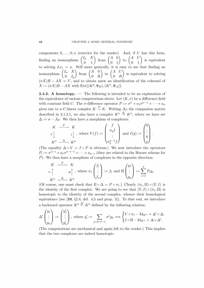
42 CHAPTER 2. SOME GENERAL NONSENSE
components 0, . . . , 0, u (exercice for the reader). And, if U has this form,
finding an isomorphism(In X
0 1
)from
(A 00 1
)to(A U
0 1
)is equivalent
to solving Lx1 = u. Still more generally, it is easy to see that finding an
isomorphism(In X
0 Ip
)from
(A 00 B
)to(A U
0 B
)is equivalent to solving
(σX)B − AX = U , and to obtain anew an identification of the cokernel ofX 7→ (σX)B −AX with Ext
((Kp,ΦB), (Kn,ΦA)
).
2.4.2. A homotopy. — The following is intended to be an explanation ofthe equivalence of various computations above. Let (K,σ) be a difference fieldwith constant field C. The σ-difference operator P := σn + a1σ
n−1 + · · ·+ an
gives rise to a C-linear complex KP→ K. Writing AP the companion matrix
described in 2.1.2.1, we also have a complex Kn ∆→ Kn, where we have set∆ := σ −AP . We then have a morphism of complexes:
KP−−−−→ K
V
y I
yKn ∆−−−−→ Kn
, where V (f) :=
f
σqf...
σn−1q f
and I(g) :=
0...0g
.
(The equality ∆ V = I P is obvious.) We now introduce the operatorsPi := σn−i + a1σ
n−i−1 + · · ·+ an−i (they are related to the Horner scheme forP ). We then have a morphism of complexes in the opposite direction:
KP−−−−→ K
π1
x Π
xKn ∆−−−−→ Kn
, where π1
f1...fn
:= f1 and Π
g1...gn
:=n∑
i=1
Pigi.
(Of course, one must check that Π ∆ = P π1.) Clearly (π1,Π) (V, I) isthe identity of the first complex. We are going to see that (V, I) (π1,Π) ishomotopic to the identity of the second complex, whence their homologicalequivalence (see [10, §2.4, def. 4,5 and prop. 5]). To that end, we introduce
a backward operator Kn ∆′← Kn defined by the following relation:
∆′
g1...gn
:=
g′1...g′n
, where g′i :=∑
j+k=i−1
σjgk =⇒
V π1 − IdKn = ∆′ ∆,
I Π− IdKn = ∆ ∆′.
(The computations are mechanical and again left to the reader.) This impliesthat the two complexes are indeed homotopic.

CHAPTER 3
THE AFFINE SPACE OF ISOFORMAL
ANALYTIC CLASSES
3.1. Isoformal analytic classes of analytic q-difference modules
We shall now specialize section 2.3, in particular subsection 2.3.6, to thecase of q-difference modules.
3.1.1. Extension classes of analytic q-difference modules. — Fromhere on, we consider only analytic q-difference modules and the base field isC(z) (except for brief indications about the formal case).
Theorem 3.1.1. — Let M,N be pure modules of ranks r, s ∈ N∗ and slopesµ < ν ∈ Q. Then dimCF(M,N) = rs(ν − µ).
Proof. — Since F(M,N) ' Ext1(N,M) ' Γ1(N∨ ⊗M), and since N∨ ⊗Mis pure isoclinic of rank rs and slope µ− ν < 0, the theorem is an immediateconsequence of the following lemma.
Lemma 3.1.2. — Let M be a pure module of ranks r and slope µ < 0. ThendimC Γ1(M) = −rµ.
Proof. — We give four different proofs, of which two require that µ ∈ Z.1) Write d := −rµ ∈ N∗. If M = Dq/DqP , the module M∨ is pure of
rank r and slope −µ, and can be written as Dq/DqP∨ for some dual P∨ =
a0 + · · · + arσrq of P , such that v0(a0) = 0, v0(ar) = d and v0(ai) ≥ id/r for
all i (lemma 2.2.3). We want to apply proposition 2.5 of [6], but the latterassumes |q| < 1, so we consider L := P∨σ−r
q = b0 + · · ·+ brσr, where σ := σ−1
q
and bi := ar−i. After loc.cit, the operator L : Cz → Cz has index d.More generally, for all m ∈ N∗, the operator L : z−mCz → z−mCz isconjugate to zmLz−m =
∑qimbiσ
i : Cz → Cz, which also has index d.Hence L : C(z) → C(z) has index d, and so has P∨. After corollary

44 CHAPTER 3. THE AFFINE SPACE OF ISOFORMAL ANALYTIC CLASSES
2.3.20, this index is dimC Γ1(M) − dimC Γ(M). But, M being pure isoclinicof non null slope, Γ(M) = 0, which ends the first proof.
2) In the following proof, we assume µ ∈ Z. From theorem 1.2.3 of [44], weknow that we may choose the dual operator such that:
P∨ = (z−µσq − c1)u1 · · · (z−µσq − cr)ur,
where c1, . . . , cr ∈ C∗ and u1, . . . , ur ∈ Cz, u1(0) = · · · = ur(0) = 1. Weare thus left to prove that each z−µσq − c1 has index −µ: the indexes add upand the sum will be −rµ = d. Since the kernels are trivial, we must computethe cokernel of an operator zmσq − c, m ∈ N∗. But it follows from lemma3.1.3 that the image of zmσq−c : C(z)→ C(z) admits the supplementaryspace C⊕ · · · ⊕Czm−1.
3) In the following proof, we assume again µ ∈ Z. After lemma 2.2.3, wecan write M = (C(z)r,ΦzµA), A ∈ GLr(C). After corollary 2.3.18, we must
consider the cokernel of C(z)r ΦzµA−Id→ C(z)r. But, after lemma 3.1.3, theimage of ΦzµA − Id admits the supplementary space (C⊕ · · · ⊕Cz−µ−1)r.
4) A similar proof, but for arbitrary µ, can be deduced from [51]. It followsindeed from this paper that each isoclinic module of slope µ can be obtained bysuccessive extensions of modules admitting a dual of the form Dq/Dq(zaσb
q−c),where b/a = −µ and c ∈ C∗.
Lemma 3.1.3. — Let d, r ∈ N∗ and A ∈ GLr(C). Let D ⊂ Z be any set ofrepresentatives modulo d, for instance a, a+1, . . . , a+d−1 for some a ∈ Z.Then, the image of the C-linear map F : X 7→ zdAσqX −X from C(z)r to
itself admits as a supplementary(∑
i∈D
Czi
)r
.
Proof. — For all i ∈ Z, write Ki := ziC(zd), so that C(z) =⊕
i∈D Ki.Each of the Kr
i is stable under F . We write w := zd, L := C(w), ρ := qd
and define σ on L by σf(w) = f(ρw). Multiplication by zi sends Lr to Kri and
conjugates the restriction of F to Kri to the mapping Gi : Y 7→ wqiAσY − Y
from Lr to itself. We are left to check that the image of Gi admits Cr as asupplementary. But this is just the case d = 1, D = 0 of the lemma. So wetackle this case under these assumptions with the notations of the lemma.
So write FA : X 7→ zAσqX − X from C(z)r to itself. Also writeX =
∑Xnz
n and Y = FA(X) =∑Ynz
n (all sums here have at mosta finite number of negative indices), so that Yn = qn−1AXn−1 − Xn.Putting X :=
∑A−nXnz
n and Y :=∑A−nYnz
n, from the relationA−nYn = qn−1A−(n−1)Xn−1 − A−nXn, we draw Y = zσqX − X. Of

3.1. ISOFORMAL ANALYTIC CLASSES OF ANALYTIC q-DIFFERENCE MODULES 45
course, X 7→ X is an automorphism of C(z)r and we just saw that itconjugates FA to the map F : X 7→ zσqX − X from C(z)r to itself.Moreover, the same automorphism leaves Cr ⊂ C(z)r, so the question boilsdown to prove that the image of F has supplementary Cr. And this, in turn,splits into r times the same problem for r = 1.
So we are left with the case of the map f 7→ zσqf − f from C(z) to itself,which is the very heart of the theory! To study the equation zσqf − f = g,one introduces the q-Borel transform of level 1, defined by the formula:
Bq,1
(∑fnz
n)
=∑ fn
qn(n−1)/2zn.
For properties of Bq,1 see [33]. It sends C(z) isomorphically to a subspaceof the space O(C)[z−1], namely, the C-vector space:
C(z)q,1 :=∑
fnzn ∈ C(z) | fn ≺ q−n(n−1)/2
.
Here, un ≺ vn means: un = O(Anvn) for some A > 0. Introduction of theq-Borel transform is motivated by the following easily checked property:
zσqf − f = g ⇐⇒ ∀n , qn−1fn−1 − fn = gn
⇐⇒ ∀n , fn−1
q(n−1)(n−2)/2− fn
qn(n−1)/2=
gn
qn(n−1)/2
⇐⇒ (z − 1)Bq,1f = Bq,1g.
We therefore get a commutative diagram:
C(z) 1−zσq−−−−→ C(z)yBq,1
yBq,1
C(z)q,1
×(1−z)−−−−−→ C(z)q,1
The vertical arrows are isomorphisms and the right one sends C ⊂ C(z) ontoC ⊂ C(z)q,1. We are going show that the image of the lower horizontalarrow is φ ∈ C(z)q,1 | φ(1) = 0. (The fact that ×(1 − z) does sendC(z)q,1 into itself is easily checked.) It will then follow that the image ofthe upper horizontal arrow is g ∈ C(z) | Bq,1g(1) = 0, that it admitsC as a supplementary and that the corresponding projection operators areg 7→ Bq,1g(1) and g 7→ g − Bq,1g(1); thus, the only obstruction in solvingzσqf − f = g analytically is Bq,1g(1) (solving formally is always possible).
It is obvious that φ(1) makes sense for any φ ∈ C(z)q,1 and so thatany φ in the image satisfies φ(1) = 0. If φ(1) = 0, it is also clear that

46 CHAPTER 3. THE AFFINE SPACE OF ISOFORMAL ANALYTIC CLASSES
ψ :=φ
1− z∈ O(C)[z−1], and we are left to prove that ψ ∈ C(z)q,1. So we
write φ =∑anz
n, ψ =∑bnz
n, so that we have∑an = 0 and:
bn =∑p≤n
ap = −∑p>n
ap.
Suppose that |an| ≤ CAn |q|−n(n−1)/2 for all n, where C,A > 0. Then:
|bn| ≤ C∑p>n
Ap |q|−p(p−1)/2 ≤ CAn |q|−n(n−1)/2∑`>0
A` |q|−`(2n+`−1)/2 ≤ C ′An |q|−n(n−1)/2 ,
where C ′ :=∑>0
A` |q|−`(`−1)/2 <∞. This achieves the proof.
Note that from the proof, one draws explicit projection maps from C(z)r
to the image of FA and its supplementary Cr: these are the maps Y 7→Y − Bq,1Y (A−1) and Y 7→ Bq,1Y (A−1), where:
Bq,1Y (A−1) :=∑
q−n(n−1)/2A−nYn.
3.1.2. The affine scheme F(P1, . . . , Pk). — Now let P1, . . . , Pk be pureisoclinic q-difference modules over C(z), of ranks r1, . . . , rk ∈ N∗ and slopesµ1 < · · · < µk. From section 2.3, we have a functor from commutative C-algebras to sets:
C ; F (C) := F(C ⊗C P1, . . . , C ⊗C Pk).
Here, the base change C⊗C− means that we extend the scalars of q-differencemodules from C(z) to C ⊗C C(z).
Theorem 3.1.4. — The functor F is representable and the correspondingaffine scheme is an affine space over C with dimension:
dimF(P1, . . . , Pk) =∑
1≤i<j≤k
rirj(µj − µi).
Proof. — We apply theorem 2.3.11. We need two check the assumptions:
∀i, js.t.1 ≤ i < j ≤ k , Hom(Pj , Pi) = 0 and dimC Ext(Pj , Pi) = rirj(µj−µi).
The first fact comes from theorem 2.2.4 and the second fact from theorem3.1.1; the fact that the extension modules are free is here obvious since C is afield.
Remark 3.1.5. — The use of base changes C ⊗C C(z) is too restrictiveto consider this as a true space of moduli: we should like to consider families

3.2. INDEX THEOREMS AND IRREGULARITY 47
of modules the coefficients of which are arbitrary analytic functions of someparameter. This will be done in a further work.
Now, to get coordinates on our affine scheme, we just have to find bases ofthe extension modules Ext(Pj , Pi) for 1 ≤ i < j ≤ k: this follows indeed fromcorollary 2.3.15. An example will be given by corollary 3.3.7.
3.2. Index theorems and irregularity
We shall now give some complements to the results in 3.1.1, in the form ofindex theorems. They mostly originate in the works [6] of Bezivin and alsoin [33]. Although not strictly necessary for what follows, they allow for aninterpretation of dimF(P1, . . . , Pk) (theorem 3.1.4) in terms of “irregularity”,as in the paper [26] of Malgrange.
In most of this section, we write K for (indifferently) C((z)) or C(z) andrespectively speak of the formal or convergent case. We intend to computethe index of an analytic q-difference operator P ∈ Dq acting upon C((z)) andC(z) (and, in the end, upon C((z))/C(z)). To begin with, we do notassume P to have analytic coefficients.
3.2.1. Kernel and cokernel of σq−u. — We start with the case degP = 1.Up to an invertible factor in Dq, we may assume that P = σq − u, whereu = dqkzνv, v ∈ K, v(0) = 1, with k ∈ Z and d ∈ C∗ such that 1 ≤ |d| < |q|.We consider P as a C-linear operator on K.
Fact. — The dimensions over C of the kernel and cokernel of P depend onlyof the class of u ∈ K∗ modulo the subgroup σq(w)
w | w ∈ K∗ of K∗. Thisclass is equal to that of a dzν .
Proof. — Conjugating the C-linear endomorphism σq − u of K by w ∈ K∗
(undestood as the automorphism ×w), one finds:
w (σq − u) w−1 =w
σq(w) (σq − u′), with u′ = u
σq(w)w
,
whence the first statement. Then, qkv = σq(w)w , where w = zk
∏i≥1σ−i
q (v) ∈ K
(also well defined in the convergent case), whence the second statement.
So we now set u := dzν .

48 CHAPTER 3. THE AFFINE SPACE OF ISOFORMAL ANALYTIC CLASSES
Fact. — The kernel of σq−u : K → K has dimension 1 if (ν, d) = (0, 1), and0 otherwise.
Proof. — The series f =∑fnz
n belongs to the kernel if, and only if∀n , qnfn = dfn−ν . Since we deal with Laurent series having poles, thisimplies f = 0 except maybe if ν = 0. In the latter case, it implies f = 0,except maybe if d ∈ qZ. From the condition on |d|, this is only possible ifd = 1, thus u = 1. In that case, the kernel is plainly C.
Fact. — The map σq − u : K → K is onto if ν > 0 and also if ν = 0, d 6= 1.
Proof. — Let g ∈ K. We look for f solving the equation σqf−dzνf = g in K.This is equivalent to: ∀n , qnfn − dfn−ν = gn, that is, ∀n , fn = q−n(dfn−ν +gn). If ν ≥ 1, one computes the coefficients by induction from the ν firstamong them. Moreover, in the convergent case, inspection of the denominatorsshow that f converges if g does; and then, the functional equation ensuresmeromorphy. If ν = 0 and d 6= 1 (so that d /∈ qZ), one gets rightaway fn =
gn
qn−d . Convergence (resp. meromorphy) is then immediate in the convergentcase. (When ν ≥ 1, one can also consider the fixpoint equation F (f) = f ,where F (f) := σ−1
q (g + dzνf): it is easy to see that this is a contractingoperator as well for the formal as for the transcendant topology.)
Fact. — If (ν, d) = (0, 1), the cokernel of σq − u : K → K has dimension 1.
Proof. — One checks that σq−u vanishes on C and induces an automorphismof the subspace K• of K made up of series without constant term.
Fact. — Assume ν < 0. Then σq − u : K → K is onto in the formal case.
Proof. — Put F ′(f) = d−1z−ν(σq(f) − g). Since ν > 0, this is a z-adicallycontracting operator, whence the existence (and unicity) of a fixed point.
Remark 3.2.1. — This is the first place where the formal and convergentcases differ. The operator is (rather strongly) expanding for the transcen-dant topology, it produces Stokes phenomena ! So this is where we need anargument from analysis in the convergent case.
Fact. — Assume ν = −r, r ∈ N∗. Then, in the convergent case, the cokernelof σq − u : K → K has dimension r.
Proof. — This is a consequence of lemma 3.1.2 (and therefore relies on theuse of the q-Borel transformation).
We now summarize our results:
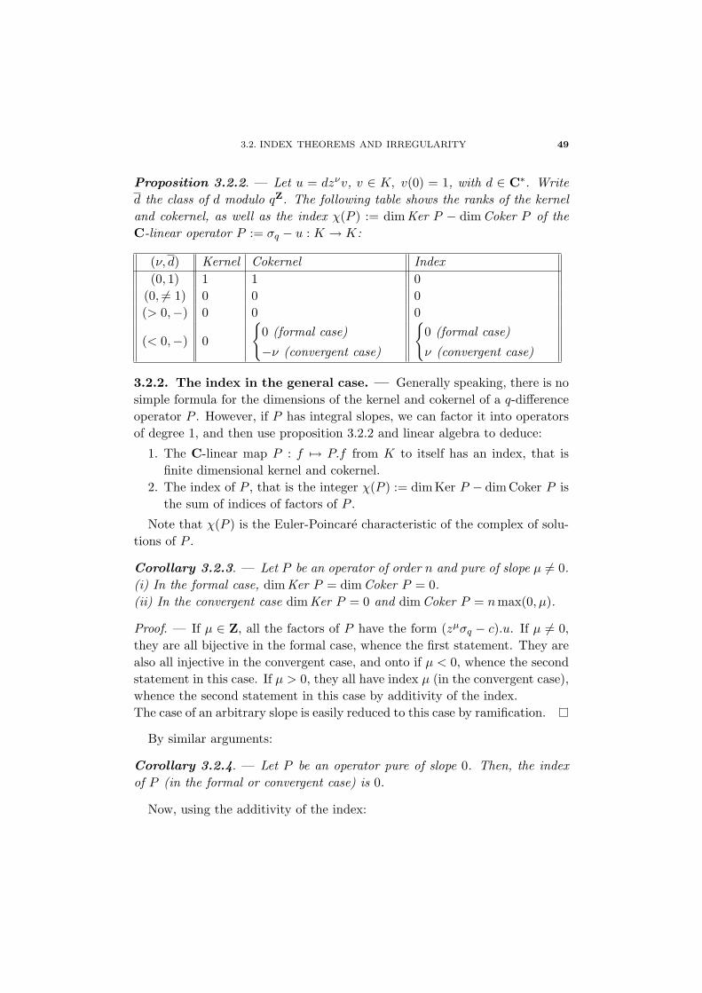
3.2. INDEX THEOREMS AND IRREGULARITY 49
Proposition 3.2.2. — Let u = dzνv, v ∈ K, v(0) = 1, with d ∈ C∗. Writed the class of d modulo qZ. The following table shows the ranks of the kerneland cokernel, as well as the index χ(P ) := dim Ker P − dim Coker P of theC-linear operator P := σq − u : K → K:
(ν, d) Kernel Cokernel Index(0, 1) 1 1 0
(0, 6= 1) 0 0 0(> 0,−) 0 0 0
(< 0,−) 0
0 (formal case)
−ν (convergent case)
0 (formal case)
ν (convergent case)
3.2.2. The index in the general case. — Generally speaking, there is nosimple formula for the dimensions of the kernel and cokernel of a q-differenceoperator P . However, if P has integral slopes, we can factor it into operatorsof degree 1, and then use proposition 3.2.2 and linear algebra to deduce:
1. The C-linear map P : f 7→ P.f from K to itself has an index, that isfinite dimensional kernel and cokernel.
2. The index of P , that is the integer χ(P ) := dim Ker P − dim Coker P isthe sum of indices of factors of P .
Note that χ(P ) is the Euler-Poincare characteristic of the complex of solu-tions of P .
Corollary 3.2.3. — Let P be an operator of order n and pure of slope µ 6= 0.(i) In the formal case, dim Ker P = dim Coker P = 0.(ii) In the convergent case dim Ker P = 0 and dim Coker P = nmax(0, µ).
Proof. — If µ ∈ Z, all the factors of P have the form (zµσq − c).u. If µ 6= 0,they are all bijective in the formal case, whence the first statement. They arealso all injective in the convergent case, and onto if µ < 0, whence the secondstatement in this case. If µ > 0, they all have index µ (in the convergent case),whence the second statement in this case by additivity of the index.The case of an arbitrary slope is easily reduced to this case by ramification.
By similar arguments:
Corollary 3.2.4. — Let P be an operator pure of slope 0. Then, the indexof P (in the formal or convergent case) is 0.
Now, using the additivity of the index:

50 CHAPTER 3. THE AFFINE SPACE OF ISOFORMAL ANALYTIC CLASSES
Corollary 3.2.5. — The index of an arbitrary operator P is 0 in the formalcase and −
∑µ>0
rP (µ)µ in the convergent case.
Corollary 3.2.6. — Let P ∈ Dq be an analytic q-difference operator. Theindex of P acting as a C-linear endomorphism of C((z))/C(z) is equal to∑µ>0
rP (µ)µ.
Of course, rP denotes here the Newton function of P introduced in subsec-tion 2.2.1.
3.2.3. Irregularity and the dimension of F(P1, . . . , Pk). — The follow-ing definition is inspired by that of [26].
Definition 3.2.7. — The irregularity of a q-difference operator P , resp. ofq-difference module M , is defined by the formulas:
Irr (P ) :=∑µ>0
rP (µ)µ, Irr (M) :=∑µ>0
rM (µ)µ.
Graphically, this is the height of the right part of the Newton polygon, fromthe bottom to the upper right end. It is clearly a formal invariant. From itsinterpretation as an index in C((z))/C(z), the irregularity of operators isadditive with respect to the product. From theorem 2.2.1, the irregularityof modules is additive with respect to exact sequences. Moreover, with thenotations of 2.2.4, writing
M>0 := M/M≤0
the “positive part” of M , one has:
Irr (M) = Irr (M>0).
Write M0 := P1 ⊕ · · · ⊕ Pk. Then the “internal End” M := End(M0) =M∨
0 ⊗M0 of this module (subsection 2.1.1) has as Newton function:
rM (µ) =∑
µj−µi=µ
rirj .
(This follows from theorem 2.2.1.) From theorem 3.1.4 and definition 3.2.7,we therefore get the equality:
dimF(P1, . . . , Pk) = Irr (End(M0)) .
In subsection 6.3.2, we shall give a sheaf theoretical interpretation of thisformula.

3.3. EXPLICIT DESCRIPTION OF F(P1, . . . , Pk) IN THE CASE OF INTEGRAL SLOPES51
3.3. Explicit description of F(P1, . . . , Pk) in the case of integral slopes
FROM NOW ON, WE ASSUME THAT THE SLOPES AREINTEGRAL: µ1, . . . , µk ∈ Z.
It is then possible to make this result more algorithmic by using thematricial description of paragraph 2.2.4.2. Indeed, as explained in paragraph1.1.3.1, our construction of normal forms and of explicit Stokes operatorsdepends on the normal form (8) given herebelow for pure modules.
For i = 1, . . . , k, we thus write Pi = (C(z)ri ,ΦzµiAi), with Ai ∈ GLri(C).Then, putting n := r1 + · · · + rk, we have M0 := P1 ⊕ · · · ⊕ Pk = (Kn,ΦA0),with A0 as in equation (5):
(8) A0 :=
zµ1A1 . . . . . . . . . . . .
. . . . . . . . . 0 . . .
0 . . . . . . . . . . . .
. . . 0 . . . . . . . . .
0 . . . 0 . . . zµkAk
.
Any class in F(P1, . . . , Pk) can be represented by a module MU := (Kn,ΦAU)
for some U := (Ui,j)1≤i<j≤k ∈∏
1≤i<j≤k
Matri,rj (C(z)), with:
(9) AU :=
zµ1A1 . . . . . . . . . . . .
. . . . . . . . . Ui,j . . .
0 . . . . . . . . . . . .
. . . 0 . . . . . . . . .
0 . . . 0 . . . zµkAk
,
and MU ,MV represent the same class if, and only if, the equation (σqF )AV =AUF can be solved with F ∈ G(C(z)). Such an F is then unique.
3.3.1. Analytic classification with 2 integral slopes. — From the re-sults of 3.1.1, we get the following result for the case of two slopes. Here, andafter, we write, for µ < ν ∈ Z:
Kµ,ν :=ν−µ−1∑
i=0
Czi or, at will: Kµ,ν :=ν−1∑i=µ
Czi.
(The second choice is motivated by good tensor properties, see for instance[32].) Then, for r, s ∈ N∗, we denote Matr,s(Kµ,ν) the space of r× s matriceswith coefficients in Kµ,ν .

52 CHAPTER 3. THE AFFINE SPACE OF ISOFORMAL ANALYTIC CLASSES
Proposition 3.3.1. — Let U ∈ Matr1,r2(C(z)). Then, there exists aunique pair:
Red(µ1, A1, µ2, A2, U) := (F1,2, V ) ∈ Matr1,r2(C(z))×Matr1,r2(Kµ1,µ2)
such that:(σqF1,2)zµ2A2 − zµ1A1F1,2 = U − V,
that is: (Ir1 F1,2
0 Ir2
):(zµ1A1 V
0 zµ2A2
)'(zµ1A1 U
0 zµ2A2
).
Proof. — Using the reductions of lemma 3.1.2, this is just a rephrasing oflemma 3.1.3.
We consider V as a polynomial normal form for the class of MU and F1,2
as the corresponding reduction datum. Of course, they depend on the choiceof the space of coefficients Kµ1,µ2 .
Example 3.3.2. — This is the archetypal example, from which much of thetheory is built. Fix c ∈ C∗. For any f, u, v ∈ C(z), the isomorphism:(
1 f
0 1
):(
1 v
0 cz
)'(
1 u
0 cz
)is equivalent to the inhomogeneous q-difference
equation: czσqf −f = u−v. Writing f =∑fnz
n, etc, we find the conditions:
cqn−1fn−1− fn = un− vn ⇐⇒fn−1
cn−1q(n−1)(n−2)/2− fn
cnqn(n−1)/2=
un − vn
cnqn(n−1)/2,
which admit an analytic solution f if, and only if, Bq,1u(c−1) = Bq,1v(c−1).
The analytic class of the module with matrix(
1 u
0 cz
)within the formal
class(
1 00 cz
)is therefore Bq,1u(c−1) ∈ C. Writing fu the unique solution in
C(z) of the equation czσqf−f = u−Bq,1u(c−1), we have Red(0, 1, 1, c, u) =(fu,Bq,1u(c−1)
).
Note that equation czσqf − f = u always admits a unique formal solutionfu. For instance, for u ∈ C, we find that fu = −uCh(cz), where Ch isthe Tshakaloff series defined by (4) page 16). We infer that, for a generalu ∈ C(z), one has fu = fu − Bq,1u(c−1)Ch(cz).
Example 3.3.3 (A direct computation). — In proposition 3.3.1, wemeet the equation (σqF1,2)zµ2A2 − zµ1A1F1,2 = U − V . Here is an explicit

3.3. EXPLICIT DESCRIPTION OF F(P1, . . . , Pk) IN THE CASE OF INTEGRAL SLOPES53
resolution that does not go through all the reductions of 3.1.1. We writeX =
∑Xnz
n for F1,2 and Y =∑Ynz
n for U − V . We have:
∀n , qn−µ2Xn−µ2A2−A1Xn−µ1 = Yn ⇐⇒ ∀n , qn−dA−11 Xn−dA2−Xn = Zn := A−1
1 Yn+µ1 ,
where we denote d := µ2 − µ1 ∈ N∗ the level of the above inhomogeneousequation. It follows from [6], [33] that, for any analytic Y , this has a formalsolution of g-Gevrey level d (this was defined in paragraph 1.3.2 of the generalnotations, in the introduction); it also follows from loc.cit that, if there is asolution of q-Gevrey level d′ > d (which is a stronger condition), then, there isan analytic solution. To solve our equation, we introduce a q-Borel transformof level d. This depends on an arbitrary family (tn)n∈Z in C∗, subject to thecondition:
∀n , tn = qn−dtn−d.
For d = 1, the natural choice is tn := qn(n−1)/2. In general, such a family canbe built from Jacobi theta functions as in [32]. At any rate, tn has the orderof growth of qn2/2d. The q-Borel transform is then defined by:
Bq,d
(∑fnz
n)
:=∑ fn
tnzn.
We must also choose dth roots B1, B2 of A1, A2. Then, writing Bq,dX =∑Xnz
n, etc, we find the relations:
∀n , B−d1 Xn−dB
d2−Xn = Zn ⇐⇒ ∀n , Bn−d
1 Xn−dB−(n−d)2 −Bn
1 XnB−n2 = Bn
1 ZnB−n2 .
Thus, a necessary condition for the existence of an analytic solution X is that,for all i in a set of representatives modulo d, one has:∑
n≡i (mod d)
Bn1 ZnB
−n2 = 0.
This provides us with d obstructions in Matr1,r2(C) and it is not hard to prove,along the same lines as what has been done, that these form a complete setof invariants. More precisely, the map which sends U to the d-uple of ma-
trices∑
n≡i (mod d)
1tnBn−d
1 Un+µ1B−n2 yields an isomorphism of F(P1, P2) with
Matr1,r2(C)d. Different choices of the family (tn) and the matrices B1, B2
induce different isomorphisms.
3.3.2. The Birkhoff-Guenther normal form. — Going from two slopesto general case rests on the following remark. The functor M ; M ′ :=M≤µk−1
induces an onto mapping F(P1, . . . , Pk) → F(P1, . . . , Pk−1). Theinverse image in F(P1, . . . , Pk) of the class of M ′ in F(P1, . . . , Pk−1) is in

54 CHAPTER 3. THE AFFINE SPACE OF ISOFORMAL ANALYTIC CLASSES
natural one-to-one correspondance with the space Ext1(Pk,M′). The latter is
a C-vector space of dimension∑
1≤j<k
rjrk(µk−µj). This follows from the slope
filtration 0 = M0 ⊂ · · · ⊂ Mk−1 = M ′ and the resulting exact sequences, for1 ≤ j < k:
0→Mj−1 →Mj → Pj → 0 =⇒ 0→ Ext1(Pk,Mj−1)→ Ext1(Pk,Mj)→ Ext1(Pk, Pj)→ 0.
(Recall that Hom(Pk, Pj) = 0.) Actually, there is a non canonical C-linearisomorphism Ext1(Pk,M
′) '⊕
1≤j<k Ext1(Pk, Pj). One can go further usingthe matricial description of paragraph 2.2.4.2. We keep the notations re-called at the beginning of subsection 3.3.1 and moreover denote MU the classin F(P1, . . . , Pk) of the module MU := (Kn,ΦAU
) for U := (Ui,j)1≤i<j≤k ∈∏1≤i<j≤k
Matri,rj (C(z)).
Proposition 3.3.4. — The map U 7→ MU from∏
1≤i<j≤k
Matri,rj (Kµi,µj ) to
F(P1, . . . , Pk) is one-to-one.
Proof. — We already now that the map is onto and the conclusion will followfrom the following fact: for all U ∈
∏1≤i<j≤k
Matri,rj (C(z)), there exists a
unique pair (F, V ) ∈ G(C(z))×∏
1≤i<j≤k
Matri,rj (Kµi,µj ) such that F [AV ] =
AU . Writing F as in equation (6) and V = (Vi,j), this is equivalent to thefollowing system:
∀(i, j), 1 ≤ i < j ≤ k , Vi,j+j−1∑
`=i+1
(σqFi,`)V`,j+(σqFi,j)(zµjAj) = (zµiAi)Fi,j+j−1∑
`=i+1
Ui,`F`,j+Ui,j .
It is understood thatj−1∑
`=i+1
= 0 when j = i + 1. Then, U being given, the
system is (uniquely) solved by induction on j − i by the following formulas:
(Fi,j , Vi,j) := Red
(µi, Ai, µj , Aj , Ui,j +
j−1∑`=i+1
Ui,`F`,j −j−1∑
`=i+1
(σqFi,`)V`,j
).
Theorem 3.3.5. — The set F(P1, . . . , Pk) is an affine space of dimension∑1≤i<j≤k
rirj(µj − µi).
Proof. — This is an immediate consequence of the proposition.
3.3. EXPLICIT DESCRIPTION OF F(P1, . . . , Pk) IN THE CASE OF INTEGRAL SLOPES55
Note that this is the area contained in the lower finite part of the Newtonpolygon. This result is the natural continuation of a normalisation processfound by Birkhoff and Guenther in [9].
Definition 3.3.6. — A matrix AU such that U := (Ui,j)1≤i<j≤k ∈∏1≤i<j≤k
Matri,rj (C(z)) will be said to be in Birkhoff-Guenther normal
form.
Now, using the argument that follows theorem 3.1.4, we draw from corollary2.3.15:
Corollary 3.3.7. — The components of the matrices (Ui,j)1≤i<j≤k make upa complete system of coordinates on the space F(P1, . . . , Pk−1).
3.3.3. Computational consequences of the Birkhoff-Guenther nor-mal form. — Let A0 be as in (8) and AU = A as in (9). Looking forF ∈ G(C((z))) such that F [A0] = A amounts, with notation (6), to solvingthe system:
∀(i, j), 1 ≤ i < j ≤ k , (σqFi,j)(zµjAj) = (zµiAi)Fi,j +j−1∑
`=i+1
Ui,`F`,j + Ui,j .
This is triangular in the sense that the equation in Fi,j depends on previouslyfound F`,j with ` > i.
Assume that A is in Birkhoff-Guenther normal form (definition 3.3.6). Thenwe can write Ui,j = zµiU ′i,j , where U ′i,j has coefficients in C[z]. The previousequation becomes:
(σqFi,j)(zµj−µiAj) = AiFi,j +j−1∑
`=i+1
U ′i,`F`,j + U ′i,j .
Assume by induction that all F`,j have coefficients in C[[z]]. Then one maywrite the above equation as:
Fi,j = U ′′ + zδA−1i (σqFi,j)Aj ,
where U ′′ has coefficients in C[[z]] and δ ∈ N∗. This is a fixpoint equationfor an operator that is contracting in the z-adic topology of C[[z]] and so itadmits a unique formal solution. Therefore we find a unique F ∈ G(C[[z]])such that F [A0] = A.

56 CHAPTER 3. THE AFFINE SPACE OF ISOFORMAL ANALYTIC CLASSES
A noteworthy consequence is that the inclusions Cz ⊂ C(z) andC[[z]] ⊂ C((z)) induce a natural identification:
GA0(C[[z]])/G(Cz) ' GA0(C((z)))/G(C(z)),
and, as a corollary, a bijection:
GA0(C[[z]])/G(Cz)→ F(P1, . . . , Pk).
3.4. Interpolation by q-Gevrey classes
We shall now extend the previous results to q-Gevrey classification. We usehere notations from paragraph 1.3.2 of the general notations in the introduc-tion.
3.4.1. q-Gevrey extension spaces. —
3.4.1.1. q-Gevrey extensions for arbitrary slopes. — If one repaces the fieldC(z) by the field C((z))q;s of q-Gevrey series of level s > 0 and Dq by Dq,s :=C((z))q;s〈T, T−1〉, one gets the abelian category DiffMod(C((z))q;s, σq) andthe following extension of the results of 3.1.1.
Proposition 3.4.1. — Let M,N be pure modules of ranks r, s ∈ N∗ andslopes µ < ν ∈ Q in DiffMod(C((z))q;s, σq). Then one has:
dimC Ext1(M,N) =
0 if ν − µ ≥ 1/s,
rs(ν − µ) if ν − µ < 1/s.
Proof. — This follows indeed, by the same arguments as before, from propo-sitions 3.2 and 3.3 of [6].
This remains true in the extreme case that s = ∞, since, over the fieldC((z)), the slope filtration splits and Ext1(M,N) = 0; and also in the extremecase that s = 0, by theorem 3.1.1. Therefore, the above proposition is aninterpolation between the analytic and formal settings.
3.4.1.2. q-Gevrey extensions for integral slopes. — Here, we extend the resultsof 3.3.1. If one replaces C(z) by C((z)), one gets V = 0 in all relations(F, V ) = Red(µ1, A1, µ2, A2, U) and the corresponding space of classes hasdimension 0. The previous algorithm then produces F = FU and the “formalnormal form” A0 of A. If one replaces C(z) by C((z))q;s, one gets V = 0and a matrix F of g-Gevrey level µ2 − µ1 if µ2 − µ1 ≥ 1/s, and the sameRed(µ1, A1, µ2, A2, U) as before otherwise.
3.4. INTERPOLATION BY q-GEVREY CLASSES 57
3.4.2. Isoformal q-Gevrey classification. —
3.4.2.1. q-Gevrey classification for arbitrary slopes. — One can state themoduli problem for q-Gevrey classification at order s, that is, over the fieldC((z))q;s of q-Gevrey series of order s > 0 (see subsection 3.4.1). From propo-sition 3.4.1, one gets, by the same argument as before:
Proposition 3.4.2. — Over C((z))q;s, the functor F is representable andthe corresponding affine scheme is an affine space over C with dimension∑1≤i<j≤k
µj−µi<1/s
rirj(µj − µi).
This remains true for s =∞ (formal setting, the space of moduli is a point)and for s = 0 (analytic setting, this is theorem 3.1.4).
3.4.2.2. q-Gevrey classification for integral slopes. — We fix s > 0 and writefor short q-Gevrey for q-Gevrey of order s. Every matrix is q-Gevrey equivalentto a matrix AU such that Ui,j = 0 for µj − µi ≥ 1/s. The slopes beingassumed to be integral, there is moreover a unique normal form with Ui,j = 0for µj − µi ≥ 1/s and Ui,j ∈ Matri,rj (Kµi,µj ) for µj − µi < 1/s.
3.4.3. Another kind of q-Gevrey interpolation. — A somewhat sym-metric problem is to describe the space of analytic classes within a fixed q-Gevrey class. This can be done in a similar way. We fix a matrix AU0 whereU0 ∈
∏1≤i<j≤k
Matri,rj (Kµi,µj ) is such that Ui,j = 0 for µj − µi ≥ 1/s (any
q-Gevrey class contains such a matrix). This characterizes a well defined q-Gevrey class and the space of analytic classes within this q-Gevrey class isan affine space of dimension
∑1≤i<j≤k
µj−µi≥1/s
rirj(µj − µi). If the slopes are integral,
one can assume that U0 is in normal form, i.e. each component Ui,j such thatµj − µi < 1/s belongs to Matri,rj (Kµi,µj ). Then each analytic class admits aunique normal form AU where U is in normal form and its components suchthat µj − µi < 1/s are the same as those of U0.

CHAPTER 4
THE q-ANALOGS OF
BIRKHOFF-MALGRANGE-SIBUYA
THEOREMS
4.1. Asymptotics
We shall need a q-analogue of asymptotics in the sense of Poincare. Inchapter 5 we shall develop a more restrictive notion of asymptotics.
The underlying idea, coming from the thesis [29] of Jose-Luis Martins, isthat an asymptotic theory is related to a dynamical system. In the “classical”case of Poincare asymptotics for ordinary differential equations, say locallyat 0 in C∗, the dynamical system is given by the action of the semi-groupΣ := e]−∞,0[; in our case, the semi-group is plainly Σ := q−N (in the case ofdifference equations there are two semi-groups: Σ := N and Σ := −N; thiswas used by J. Roques in [41]). Likewise, the sheaves of functions admittingan asymptotic expansion will be defined on the horizon, that is on the quotientspace C∗/Σ. In the classical case, this is the circle S1 of directions (rays from0) in C∗; in our case, this is the elliptic curve Eq = C∗/qZ = C∗/q−N (in thedifference case this is a pair of cylinders).
4.1.1. q-Asymptotics. — We set Σ := q−N and for A ⊂ C, Σ(A) :=⋃a∈A
q−Na.
Let U be an open set of C invariant by the semi-group Σ := q−N. Weshall say that a Σ-invariant subset K of U is a strict subset if there existsa compact subset K ′ of U such that K = Σ(K ′); then K∪0 is compact in C.
Let f be a function holomorphic on U and f =∑n≥0
anzn ∈ C[[z]]. We shall
say that f is q-asymptotic to f on U if, for all n ∈ N and every Σ-invariant

60 CHAPTER 4. THE q-ANALOGS OF BIRKHOFF-MALGRANGE-SIBUYA THEOREMS
strict subset K ⊂ U :
z−n(f(x)− Sn−1f
)is bounded on K. Here, Sn−1f :=
n−1∑p=0
apzp stands for ”truncation to n
terms” of f . If f admits a q-asymptotic expansion it is plainly unique. In thefollowing we will say for simplicity “asymptotic expansion” for “q-asymptoticexpansion”. For n ∈ N we shall denote f (n)(0) := n!an.
We shall denote A (U∞) the space of holomorphic functions admitting aq-asymptotic expansion on U , A0(U∞) the subspace of A (U∞) made up of(infinitely) flat functions, i.e. those such that f = 0, B(U∞) the space ofholomorphic functions bounded on every stable strict subset of U . If f isholomorphic on U , then f ∈ A (U∞) if and only if z−n
(f(x)−Sn−1f
)∈ B(U∞)
for all n ∈ N. We check easily that A (U∞) is a C-algebra and that A0(U∞)is an ideal of A (U∞).
Lemma 4.1.1. — Let U ⊂ C be a Σ-invariant open set and K ⊂ V be aΣ-invariant strict subset of U . There exists a real number ρ > 0 such that theclosed disc of radius ρ |z| and center z lies in U for all z ∈ K. Moreover it ispossible to choose ρ > 0 such that
⋃z∈K
D(z, ρ |z|) be a Σ-invariant strict subset
of U .
Proof. — There exists by definition a subset K ′ of K, compact in U , such thatK = Σ(K ′). By compacity the result of the lemma is true for every z ∈ K ′;using the action of Σ we get that it is also true for all z ∈ K.
Let f ∈ A (U∞) and f :=∑n≥0
anzn its asymptotic expansion. We set
Rn := z−n(f − Sn−1f
). We have f =
n∑p=0
apzp + zn+1Rn+1 therefore:
f ′ =n∑
p=1
papzp−1 + (n+ 1)znRn+1 + zn+1R′n+1.
If K ⊂ U is a Σ-invariant strict subset, then Rn+1 is bounded by MK,n+1 onK. Therefore, using Cauchy formula for the derivative and lemma 4.1.1, R′nis bounded by some positive constant MK,n+1
ρ|z| on K.

4.1. ASYMPTOTICS 61
We have f ′ =∑n≥1
nanzn−1 and:
z−n(f ′(x)− Sn−1f ′
)= z−n
f ′(x)−n∑
p=1
napzp−1
= (n+ 1)Rn+1 + zR′n+1.
Since∣∣(n+ 1)Rn+1 + zR′n+1
∣∣ ≤ (n+ 1 + 1ρ
)MK,n+1, then z−n
(f ′(x)−Sn−1f ′
)is bounded on K, so that f ′ admits f ′ as a q-asymptotic expansion on U .Hence A (V∞) is a differential algebra and A0(V∞) is a differential ideal ofA (V∞).
4.1.2. Asymptotic expansions and C∞ functions in Whitney sense.—
Lemma 4.1.2. — Let U be a Σ-invariant open set of C and f ∈ A (U∞).Let K ⊂ U be an invariant strict subset.
(i) There exists a positive constant CK (depending on f) such that, for allz1, z2 ∈ K ∪ 0:
|f(z1)− f(z2)| ≤ CK |z1 − z2| .
(ii) For all n ∈ N there exists a positive constant CK,n (depending on f)such that, for all z1, z2 ∈ K ∪ 0:∣∣∣∣∣∣f(z1)−
n∑p=0
f (p)(z2)p!
(z1 − z2)p
∣∣∣∣∣∣ ≤ CK,n |z1 − z2|n+1 .
(iii)
limz1→0,z2→0
z1,z2∈K∪0,z1 6=z2
1|z1 − z2|n
f(z1)−n∑
p=0
f (p)(z2)p!
(z1 − z2)p
= 0.
Proof. — (i) We choose ρ > 0 (depending on K) as in lemma 4.1.1; thenK1 :=
⋃z∈K
D(z, ρ |z|) is an invariant strict subset of U . We set:
MK := supz∈K
|f(z)− f(0)||z|
, M ′K1
:= supz∈K1
∣∣f ′(z)∣∣ .Let z1, z2 ∈ K ∪ 0. We shall consider separately three cases: (a) z2 = 0;
(b) z2 6= 0 and |z1 − z2| ≤ ρ |z2|; (c) z2 6= 0 and |z1 − z2| > ρ |z2|.The cases (a) and (b) are easy. In fact, if z2 = 0, then:
|f(z1)− f(z2)| = |f(z1)− f(0)| ≤MK |z1| = MK |z1 − z2| .

62 CHAPTER 4. THE q-ANALOGS OF BIRKHOFF-MALGRANGE-SIBUYA THEOREMS
If z2 6= 0 and |z1 − z2| ≤ ρ |z2|, then z2 ∈ K and the closed interval [z1, z2] iscontained in K1; therefore:
|f(z1)− f(z2)| ≤M ′K1|z1 − z2| .
Now consider case (c). If z2 ∈ K and |z1 − z2| > ρ |z2|, then we writef(z1)− f(z2) = f(z1)− f(0)−
(f(z2)− f(0)
)and we have:
|f(z1)− f(0)| ≤MK |z1| ≤MK
(|z2|+ |z1 − z2|
)≤(
1ρ
+ 1)MK |z1 − z2|
and
|f(z2)− f(0)| ≤MK |z2| ≤1ρMK |z1 − z2| ,
whence:
|f(z1)− f(z2)| ≤ 2 + ρ
ρMK |z1 − z2| .
Last, let CK := max(M ′
K1, 2+ρ
ρ MK
); then, for all z1, z2 ∈ K ∪ 0, we
have:
|f(z1)− f(z2)| ≤ CK |z1 − z2| .
(ii) We define ρ, K1, CK as in (i). We set:
CK,n := supz∈K
∣∣∣∣∣∣f(z)−n∑
p=0
f (p)(0)p!
zp
∣∣∣∣∣∣ ∣∣z−n−1∣∣ , M ′
K1,n := supz∈K1
∣∣∣f (n+1)(z)∣∣∣ .
The result is obviously true if f is a polynomial. Therefore, fixing n ∈ N itsuffices to prove the result when f = zn+1g, g ∈ A (U∞).
As in (i) we shall consider separately the three cases (a), (b), (c). If z2 = 0,then the result merely comes from the following relation:∣∣∣∣∣∣f(z1)−
n∑p=0
f (p)(z2)p!
(z1 − z2)p
∣∣∣∣∣∣ =
∣∣∣∣∣∣f(z1)−n∑
p=0
f (p)(0)p!
zp1
∣∣∣∣∣∣ ≤ CK,n |z1|n+1 .
Next, if z2 6= 0 and |z1 − z2| ≤ ρ |z2|, then the closed interval [z1, z2] iscontained in K1, so that:∣∣∣∣∣∣f(z1)−
n∑p=0
f (p)(z2)p!
(z1 − z2)p
∣∣∣∣∣∣ ≤M ′K1,n |z1 − z2|
n+1 .
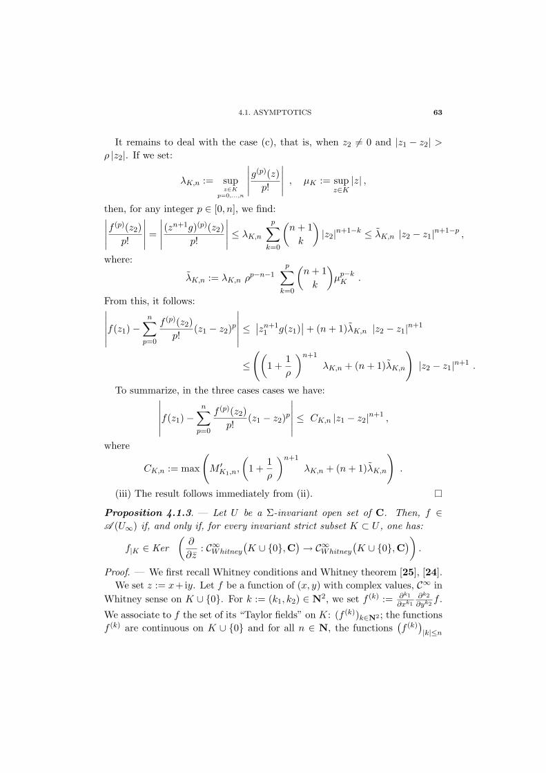
4.1. ASYMPTOTICS 63
It remains to deal with the case (c), that is, when z2 6= 0 and |z1 − z2| >ρ |z2|. If we set:
λK,n := supz∈K
p=0,...,n
∣∣∣∣∣g(p)(z)p!
∣∣∣∣∣ , µK := supz∈K|z| ,
then, for any integer p ∈ [0, n], we find:∣∣∣∣∣f (p)(z2)p!
∣∣∣∣∣ =
∣∣∣∣∣(zn+1g)(p)(z2)p!
∣∣∣∣∣ ≤ λK,n
p∑k=0
(n+ 1k
)|z2|n+1−k ≤ λK,n |z2 − z1|n+1−p ,
where:
λK,n := λK,n ρp−n−1
p∑k=0
(n+ 1k
)µp−k
K .
From this, it follows:∣∣∣∣∣∣f(z1)−n∑
p=0
f (p)(z2)p!
(z1 − z2)p
∣∣∣∣∣∣ ≤ ∣∣zn+11 g(z1)
∣∣+ (n+ 1)λK,n |z2 − z1|n+1
≤
((1 +
1ρ
)n+1
λK,n + (n+ 1)λK,n
)|z2 − z1|n+1 .
To summarize, in the three cases cases we have:∣∣∣∣∣∣f(z1)−n∑
p=0
f (p)(z2)p!
(z1 − z2)p
∣∣∣∣∣∣ ≤ CK,n |z1 − z2|n+1 ,
where
CK,n := max
(M ′
K1,n,
(1 +
1ρ
)n+1
λK,n + (n+ 1)λK,n
).
(iii) The result follows immediately from (ii).
Proposition 4.1.3. — Let U be a Σ-invariant open set of C. Then, f ∈A (U∞) if, and only if, for every invariant strict subset K ⊂ U , one has:
f|K ∈ Ker(∂
∂z: C∞Whitney
(K ∪ 0,C
)→ C∞Whitney
(K ∪ 0,C
)).
Proof. — We first recall Whitney conditions and Whitney theorem [25], [24].We set z := x+ iy. Let f be a function of (x, y) with complex values, C∞ in
Whitney sense on K ∪ 0. For k := (k1, k2) ∈ N2, we set f (k) := ∂k1
∂xk1
∂k2
∂yk2f .
We associate to f the set of its “Taylor fields” on K: (f (k))k∈N2 ; the functionsf (k) are continuous on K ∪ 0 and for all n ∈ N, the functions
(f (k)
)|k|≤n
64 CHAPTER 4. THE q-ANALOGS OF BIRKHOFF-MALGRANGE-SIBUYA THEOREMS
satisfy the following conditions, that are called Whitney conditions of ordern ∈ N and that we shall denote Wn(K):(10)
lim1
| |(x1 − x2, y1 − y2)| |n−|k|
f (k)(x1, y1)−∑|h|≤n
f (k+h)(x2, y2)h!
(x1 − x2, y1 − y2)h
= 0,
where the limit is taken for (x1, y1)→ 0, (x2, y2)→ (0, 0), with (x1, y1), (x2, y2) ∈K ∪ 0 and (x1, y1) 6= (x2, y2).
Conversely a family(f (k)
)k∈N2 of continuous functions on K ∪ 0 is
the family of Taylor jets of an element of C∞Whitney
(K ∪ 0
)if and only if
it satisfies Whitney conditions Wn(K) for all n ∈ N (this is Whitney theorem).
Using ∂∂z , ∂
∂z instead of ∂∂x , ∂
∂y , for all n ∈ N we can replace Whitneyconditions Wn(K) by equivalent conditions Wn(K).
We now return to the proof of the proposition.Let f ∈ C∞Whitney
(K ∪ 0,C
). If for all invariant strict subset K ⊂ U , one
has:
f|K ∈ Ker(∂
∂z: C∞Whitney
(K ∪ 0,C
)→ C∞Whitney
(K ∪ 0,C
)),
then, the function f is holomorphic on V , its Taylor jet f at 0 is formallyholomorphic, f =
∑n≥0
anzn and f is asymptotic to f on V , f ∈ A (U∞).
Conversely let f ∈ A (U∞); then, for all p ∈ N, f (p) ∈ A (U∞) and for allr ∈ N∗, we have ∂r
∂zr f (p) = 0.We can apply lemma 4.1.2 to each function f (p), p ∈ N, to the effect that f
satisfies conditions Wn(K) for all n ∈ N (this is assertion (iii) of the lemma);therefore it satisfies also Whitney conditions Wn(K) for all n ∈ N and, usingWhitney theorem, we get f ∈ C∞Whitney
(K ∪ 0,C
).
4.1.3. Asymptotics and sheaves on Eq. — Recall from the introductionthat we denote p : C∗ → Eq the quotient map.

4.2. EXISTENCE OF ASYMPTOTIC SOLUTIONS 65
A stable open subset U of C∗ has a “horizon” U∞ and two compactificationsU , U defined as follows:
U∞ := p(U) ⊂ Eq,
U := U ∪ 0 ⊂ C,
U := U ∪ U∞,
An invariant subset K ⊂ U is strict if and only if p(K) is a compact subsetof Eq.
We then define sheaves on Eq by putting:
– B(U∞) = the space holomorphic functions bounded on every stable strictsubset of U .
– A (U∞) = the space of holomorphic functions admitting an asymptoticexpansion f =
∑apz
p, i.e.:
∀n , z−n(f − Sn−1f) ∈ B(U∞).
– A0(U∞) = the subspace of A (U∞) made up of flat functions, i.e. thosesuch that f = 0.
Although much weaker than the q-Gevrey theorem of Borel-Ritt 5.3.3, thefollowing result does not directly flow from it, and we give here a direct proof.
Theorem 4.1.4 (Weak q-analogue of Borel-Ritt)The natural map from A to the constant sheaf C[[z]] is onto.
Proof. — Starting from an open set V ⊂ Eq small enough that U := p−1(V ) ⊂C∗ is a disjoint union of open sets Un := qnU0, where U0 is mapped homeo-morphically to V by p, we divide C∗ in a finite number of sectors Si such thateach Un is contained in one of the Si. Now, let f ∈ C[[z]]. Apply the classicalBorel-Ritt theorem within each sector Si, yielding a map fi holomorphic andadmitting the asymptotic expansion f . Glueing the fi provides a section ofA over V having image f .
4.2. Existence of asymptotic solutions
We call adequate an open subset C∗ of the form q−NU0, where theq−kU0, k ≥ 0 are pairwise disjoint. Clearly, A0(U∞) is a C(z)-vectorspace stable under σq. In particular, any q-difference operator P :=σn
q + a1σn−1q + · · · + an ∈ Dq defines a C-linear endomorphism P : f 7→
Pf = σnq (f) + a1σ
n−1q + · · · + anf of A0(U∞). Likewise, any matrix
66 CHAPTER 4. THE q-ANALOGS OF BIRKHOFF-MALGRANGE-SIBUYA THEOREMS
A ∈ GLn(C(z)), defines a C-linear endomorphism σq−A : X 7→ σqX−AXof A0(U∞)n.
Theorem 4.2.1 (Existence of asymptotic solutions)Let A ∈ GLn(C(z)) and let X ∈ C[[z]]n a formal solution of the system
σqX = AX. For any adequate open subset U , there exists a solution X ∈A (U∞)n of that system which is asymptotic to X.
Proof. — From theorem 4.1.4, there exists Y ∈∈ A (U∞)n which is asymptoticto X (without however being a solution of the system). Set:
W := σqY −AY = σq(Y − X)−A(Y − X) ∈ A0(U∞)n.
From proposition 4.2.2 below, there exists Z ∈ A0(U∞)n such that σqZ−AZ =W . Then X := Y − Z ∈ A (U∞)n is asymptotic to X and solution of thesystem.
Proposition 4.2.2. — Let A ∈ GLn(C(z)) and let U be an adequate opensubset. Then, the endomorphism σq −A of A0(U∞)n is onto.
Proof. — Let F ∈ GLn(C(z)) and B := F [A]. From the commutativediagram:
A0(U∞)n σq−A−−−−→ A0(U∞)nyF
yσqF
A0(U∞)n σq−B−−−−→ A0(U∞)n
in which the vertical arrows are isomorphisms, we just have to prove thatσq − B is onto. After the cyclic vector lemma (lemma 2.1.1), we can takeB := AP , the companion matrix of P := σn
q + a1σn−1q + · · ·+ an described in
2.1.2.1. We then apply lemma 4.2.3 (herebelow) and theorem 4.2.5 (furtherbelow).
Lemma 4.2.3. — Let R a C(z) vector space on which σq operates. Withthe notations of the previous proposition, P : R → R is onto if, and only if,σq −AP : Rn → Rn is onto.
Proof. — (i) Assume P is onto. To solve (σq − AP )
x1...xn
=
y1...yn
, put
xi+1 := σqxi − yi; one sees that x1 just has to be solution of an equationPx1 = z, where z is some explicit expression of the yi.

4.2. EXISTENCE OF ASYMPTOTIC SOLUTIONS 67
(ii) Assume σq − AP is onto. To solve Pf = g, it is enough to solve σqX −
APX =
0...0g
and to set f to the first component of X.
Remark 4.2.4. — This computation is directly related to the homotopy ofcomplexes discussed in 2.4.2.
Theorem 4.2.5. — The endomorphism P of A0(U∞) is onto.
Proof. — We give the proof under the assumption that the slopes are integral,which is the only case we need in this paper; the reader will easily deduce thegeneral case by ramification. The counterpart of the slope filtration on theside of q-difference operators is the existence of a factorisation [27, 47, 53] ofP as a product of non commuting factors: elements of Cz∗ (which induceautomorphisms of A0(U∞)) and first order operators zµσq−a, µ ∈ Z, a ∈ C∗.We are therefore reduced to the following lemma. (This is where some analysiscomes in !)
Lemma 4.2.6. — The endomorphism f 7→ zµσqf − af of A0(U∞) is onto.
Proof. — Write L this endomorphism. Let h ∈ A0(U∞); for all n ∈ N andeach strict stable subset V of U , there exists Cn,V > 0 such that |h(z)| <Cn,V |z|n over V . We distinguish two cases: (i) µ ≤ 0; (ii) µ > 0.
Case (i): µ ≤ 0 (easy case). Let Φ the automorphism of A0(U∞) definedby Φ(f) := aqµz−µσq−1f ; one has Φmf = amqµm(m+1)/2z−mµσq−mf for allm ≥ 0. Since |h(z)| ≤ Cn,V |z|n on each stable strict subset V of U and allintegers n ≥ 0, one finds:
∀z ∈ V ,∑m≥0
|Φmh(z)| ≤ Cn,V
∑m≥0
|a|m |q|µm(m+1)/2 |q|−nm |z|n .
One deduces that the series∑
m≥0 Φmh defines a flat function over U , writeit H ∈ A0(U∞). Observing that LH = zµσq(H − ΦH) = zµσqh, we see thatL is onto over A0(U∞).
Case (ii): µ > 0 (hard case). For all j ∈ N, set Uj := q−jU0 = z ∈C∗ | qjz ∈ U0; these are pairwise disjoint since U was assumed to be adequate.We are going to build successively f0, f1, f2, . . . over U0, U1, U2, . . ., which willgive rise to a function f defined over U = q−NU0, with fj = f|Uj
and Lf = h.
68 CHAPTER 4. THE q-ANALOGS OF BIRKHOFF-MALGRANGE-SIBUYA THEOREMS
For all j ∈ N, let hj := h|Uj: Uj → C. Since (σqf)|Uj
= σqfj−1, equationLf = h is equivalent to system:
∀j ∈ N∗ , zµσqfj−1 − afj = hj ,
also written:
(11) ∀j ∈ N∗ , fj = (zµσqfj−1 − hj)/a.
We agree that f−1 ≡ 0 and f0 = h0/a. Iterating the last relation (11) above,we find:
(12) ∀j ∈ N∗ , fj = −j∑
`=0
qµ`(`−1)/2z`µσ`qhj−` a
−`−1.
Write f the function defined on U by the relations f|Uj= fj , j ∈ N; Clearly,
Lf = h on U . We are left to show that f ∈ A0(U∞).Let n ∈ N and V a strict stable subset of U ; let Vj := Uj ∩ V and choose a
K > 0 such that |z| ≤ K |q|−j for all z ∈ Uj ; one has |z| ≤ K|q|−j on each Vj .Bounding by above the right hand side of (12), one gets:
(13) ∀z ∈ Vj , |fj(z)| ≤Cn,V
aPj(|q|n α) |z|n ,
where α := Kµ/a and where Pj denotes the polynomial with positive coeffi-cients:
Pj(X) :=j∑
`=0
|q|µ`(`−1)/2−j`µ X`.
Taking in account the relation
Pj+1(X) = Pj(|q|−µX) + |q|−µ(j+1)(j+2)/2 Xj+1 ,
one finds that Pj(X) ≤ P (X;µ, q) for all X > 0, where we write P (z;µ, q) theentire function defined by:
P (z;µ, q) :=∞∑
j=0
|q|−µj(j+1)/2 zj .
Said otherwise, (13) can be written in the form:
∀z ∈ Vj , |fj(z)| ≤Cn,V
aP (|q|n α;µ, q) |z|n ,
which allows us to conclude that f is flat.
We now apply theorem 4.2.1 to a situation that we shall meet when weprove theorem 4.4.1.

4.3. THE FUNDAMENTAL ISOMORPHISM 69
Let A0 ∈ GLn(C(z)) the matrix of a pure module and let A ∈GLn(C(z)) a matrix formally equivalent to A0. Let F ∈ GLn(C((z))) agauge transform proving this equivalence, i.e. F [A0] = A. (Note that wedo not assume F ∈ G(C((z))).) The conjugation relation is equivalent toσqF = AFA−1
0 , which we regard as a q-difference system of rank n2 in thespace Matn(C(z)) ' Kn2
. After theorem 4.2.1, there exists over each ade-quate open set U a solution FU ∈ Matn(C(z)) of the system σqF = AFA−1
0
that is asymptotic to F . Since the latter is invertible, and since detFU isobviously asymptotic to det F , whence non zero, FU is invertible.
Now let U ′ another adequate open set which meets U . Then U ′′ := U ∩U ′ isadequate and the matrix G := F−1
U FU ′ satisfies the two following properties:
1. It is an automorphism of A0, i.e. G[A0] = A0.2. It is asymptotic to F−1F = In, i.e. the coefficients of G − In belong to
A0(U ′′∞).
Lemma 4.2.7. — The matrix G belongs to G(A0(U ′′∞)).
Proof. — With the usual notations for A0, each block of G satisfies:
σqGi,j = (zµjAj)−1Gi,j (zµiAi) = zµi−µjA−1
j Gi,jAi.
The order of growth or decay of Gi,j near 0 is therefore the same as θqµi−µj .
Since Gi,j is flat for i 6= j, this implies Gi,j = 0 for i > j. For i = j, we applythe same argument to Gi,i − Iri , which therefore vanishes.
4.3. The fundamental isomorphism
We write ΛI := In + Matn(A0) for the subsheaf of groups of GLn(A ) madeup of matrices infinitely tangent to the identity and, if G is an algebraicsubgroup of GLn(C), we put ΛG
I := ΛI ∩ G(A ). In particular ΛGI is a sheaf
of triangular matrices of the form (6) with all the Fi,j infinitely flat.
For a q-difference module M = (C(z)n,ΦA) (section 2.1.1), we considerthe set of automorphisms of M infinitely tangent to the identity : this is thesubsheaf ΛI(M) of ΛI whose sections satisfy the equality: F [A] = A (recallthat by definition F [A] = (σqF )AF−1); this is also called the Stokes sheaf ofthe module M .

70 CHAPTER 4. THE q-ANALOGS OF BIRKHOFF-MALGRANGE-SIBUYA THEOREMS
If the matrix A has the form (5), then ΛI(M) is a subsheaf of ΛGI . Up to
an analytic gauge transformation, we can assume that we are in this case. Asa consequence, ΛI(M) is a sheaf of unipotent (and even triangular) groups.
4.3.1. Study of H1(Eq; ΛI). — We set q = e−2iπτ , =(τ) > 0 and for v ∈ R,we denote qv = e−2iπτv. We get a splitting:
C∗ = U× qR
and the map p0 : (u, v) 7→ e2iπ(u+vτ) induces an isomorphism betweenC/(Z + Zτ) and Eq = C∗/qZ.
We will call open parallelogram of Eq the image by the map p0 of an openparallelogram:
u+ vτ ∈ C | u1 < u < u2, v1 < v < v2,
where u2 − u1 ≤ 1, v2 − v1 ≤ 1 and closed parallelogram the closure of anopen parallelogram such that u2 − u1 < 1, v2 − v1 < 1. We will say that aparallelogram is small if u2 − u1 < 1/4 and v2 − v1 < 1/4.
For every open covering V of Eq, there exists a finite open covering U =(Ui)i∈I , finer than V, such that:
(i) the Ui are open parallelograms,(ii) the open sets Ui are four by four disjoint.
We will call good such a covering. There is a similar definition for closedcoverings.
– Every element of Hj(Eq; GLn(A )), j = 0, 1 can be represented by anelement of Hj(U; GLn(A )), where U is a good covering.
– The natural map Hj(U; GLn(A )) → Hj(Eq; GLn(A )) is always injec-tive.
Let U be a good open covering of Eq; we denote by C 0(U; GLn(A )) thesubspace of the space of 0-cochains (gi) ∈ C0(U; GLn(A )) whose coboundary(gij = gig
−1j ) belongs to C1(U; ΛI). It is equivalent to say that the natural
image of the cochain (gi) in C0(Eq; GLn
(C[[z]]
)) is a cocycle, or that the gi
(i ∈ I) admit the same asymptotic expansion g ∈ GLn
(C[[z]]
). We have two
natural maps:C 0(U; GLn(A ))→ Z1(U; ΛI)
C 0(U; GLn(A ))→ GLn
(C[[z]]
).
4.3. THE FUNDAMENTAL ISOMORPHISM 71
Two cochains (gi), (g′i) ∈ C 0(U; GLn(A )) define the same element ofH1(U; ΛI) if and only if:
g′ig′−1j = higig
−1j h−1
j , with (hi) ∈ C0(U; ΛI).
This is equivalent to g′−1j hjgj = g′−1
i higi, which thus defines an element f ∈H0(U; GLn(A )
)and we have g′ = hgf−1.
Lemma 4.3.1. — (i) Let U be a good open covering of Eq. The coboundarymap ∂ induces an injection on the double quotient:
C0(U; ΛI)\C 0(U; GLn(A ))/H0(U; GLn(A )
)→ H1(U; ΛI).
(ii) We have a canonical injection:
lim−→U
C0(U; ΛI)\C 0(U; GLn(A ))/GLn
(Cz
)→ H1(Eq; ΛI),
where the direct limit is indexed by the good coverings.
Proposition 4.3.2. — For every good open covering U of Eq we have a nat-ural isomorphism:
C0((U : ΛI)\C 0(U; GLn(A ))/H0(U; GLn(A )
)→ GLn
(C[[z]]
)/GLn
(Cz
).
Let U be a good open covering of Eq. Let g ∈ GLn
(C[[z]]
). Using the
q-analog of Borel-Ritt (theorem 4.1.4), we can represent it by an element gi
on each open set Ui such that gi admits g as asymptotic expansion, thereforethe natural map:
C 0(U; GLn(A ))→ GLn
(C[[z]]
)is onto. The proposition follows.
Corollary 4.3.3. — For every good open covering U of Eq, we have naturalinjections:
GLn
(C[[z]]
)/GLn
(Cz
)→ H1(U; ΛI)→ H1(Eq; ΛI).
We will see later that these maps are bijections.
4.3.2. Geometric interpretation of the elements of H1(Eq; ΛI). — Weneed some results on regularly separated subsets of the euclidean space R2.We first recall some definitions.
If X ⊂ Rn is a closed subset of the euclidean space Rn, we denote by E (X)the algebra of C∞ functions in Whitney sense on X (cf. [25]).
We recall the Whitney extension theorem: if Y ⊂ X are closed subset ofRn, the restriction map E (X)→ E (Y ) is surjective.

72 CHAPTER 4. THE q-ANALOGS OF BIRKHOFF-MALGRANGE-SIBUYA THEOREMS
Let A,B two closed sets of Rn; we define the following maps:
α : f ∈ E (A ∪B) 7→ (f|A, f|B) ∈ E (A)⊕ E (B),
β : (f, g) ∈ E (A)⊕ E (B) 7→ f|A∩B − g|A∩B ∈ E (A ∩B),
and we consider the sequence:
(14) 0→ E (A ∪B) α→ E (A)⊕ E (B)β→ E (A ∩B)→ 0.
Definition 4.3.4. — Two subsets A and B of the euclidean space Rn areregularly separated if the above sequence is exact.
The following result is due to Lojasiewicz (cf. [25]).
Proposition 4.3.5. — Let A,B two closed subsets A and B of the euclideanspace Rn; the following conditions are equivalent:
(i) A and B are regularly separated;(ii) A∩B = ∅ or for all x0 ∈ A∩B, there exists a neighborhood U of x0 and
constants C > 0, λ > 0 such that for all x ∈ U :
d(x,A) + d(x,B) ≥ Cd(x,A ∩B)λ;
(iii) A∩B = ∅ or for all x0 ∈ A∩B, there exists a neighborhood U of x0 anda constant C ′ > 0 such that for all x ∈ A ∩ U :
d(x,B) ≥ C ′d(x,A ∩B)λ.
If we can choose λ = 1 in the above condition(s), we will say that the closedsubsets A and B are transverse. Transversality is in fact a local condition.
Lemma 4.3.6. — Let K1, K2 two closed small parallelograms of Eq. Thesets p−1(K1) and p−1(K2) are transverse.
Proof. — We set:
A := p−1(K1), A0 := p−10 (A), B := p−1(K2) and B0 := p−1
0 (B)
Since K1 and K2 are small parallelograms, both A0 and B0 are formed of afamily of disjoint rectangles, that is to say:
A0 =⋃
m,n∈Z
Am,n and B0 =⋃
m,n∈Z
Bm,n,
where the families (Am,n)m,n∈Z, (Bm,n)m,n∈Z are such that d(Am,n, Am′,n′) ≥3/4 and d(Bm,n, Bm′,n′) ≥ 3/4 for any (m′, n′) 6= (m,n). We only need to dealwith the case when A∩B 6= ∅, that is, when there exists (m,n), (m′, n′) suchthat Am,n ∩Bm′,n′ 6= ∅.
4.3. THE FUNDAMENTAL ISOMORPHISM 73
Consider the function f defined over C∗ \A ∩B by
f(x) =d(x,A) + d(x,B)d(x,A ∩B)
and observe that f is q-invariant; therefore, it is enough to prove the followingstatement: for any x0 ∈ A ∩ B such that 1 < |x0| ≤ |q|, there exists anopen disk D(x0, r), r > 0, and a constant C > 0 such that f(x) ≥ C for allx ∈ D(x0, r) \ (A ∩B).
On the other hand, the mapping p0 (introduced at the beginning of 4.3.1)is a local diffeomorphism from R2 onto C∗ inducing a local equivalence be-tween the natural metrics. Therefore the proof of the lemma boils down to thetransversality between A0 and B0, which is merely deduced from the transver-sality of each pair of rectangles (Am,n, Bm′,n′) of the euclidean plane.
Let γ ∈ H1(Eq; ΛI), we can represent it by an element g ∈ Z1(U; ΛI) whereU is a good open covering of Eq. We can suppose that all the parallelogramsof the covering are small. We will associate to g a germ of fibered space(Mg, π, (C, 0)
). We will see that if we change the choice of g, then these
germs of linear fibered space correspond by a canonical isomorphism. Thisconstruction mimicks a construction of [28] inspired by an idea of Malgrange(cf. [24]), it is a central point for the proof of one of our main results.
Let g ∈ Z1(U; ΛI). We interpret the gi as germs of holomorphic functions onthe germ of q−N-invariant open set defined by Ui, that is the germ of p−1(Ui)∩D (D being an open disk centered at the origin). For sake of simplicity wewill denote also by Ui this germ. We consider the disjoint sum
∏i∈I
Ui × Cn
and (using representatives of germs) we identify the points (x, Y ) ∈ Ui ×Cn
and (x, Z) ∈ Uj ×Cn if x ∈ Uij and Z = gij(x)(Y ) (we verify that we have anequivalence relation using the cocycle condition), we denote the quotient byMg. If x = 0, gi(0) is the identity of Cn therefore the quotient Mg is a germof topological space along 0 ×Cn.
Lemma 4.3.7. — (i) The projections Ui×Cn → Ui induce a germ of con-tinuous fibration π : Mg → (C, 0), the fiber π−1(0) is identified with(Cn, 0).
(ii) The germ Mg := Mg \ π−1(0) admits a natural structure of germ ofcomplex manifold of dimension n + 1, it is the unique structure suchthat the natural injections (Ui \ 0)×Cn → Mg are holomorphic. Therestriction of π to Mg is holomorphic.

74 CHAPTER 4. THE q-ANALOGS OF BIRKHOFF-MALGRANGE-SIBUYA THEOREMS
The proof of the lemma is easy.
Lemma 4.3.8. — There exists on Mg a unique structure of germ of differ-entiable manifold (C∞) such that the natural injections (Ui \ 0)×Cn → Mg
are C∞ (in Whitney sense). The induced structure on Mg is the underlyingstructure of the holomorphic structure on Mg. The map π is C∞ of rank one,(Mg, π, (C, 0)
)is a germ of vector bundle.
Proof. — This lemma is the central point. The proof uses the Whitney ex-tension theorem and the notion of regularly separated closed sets (cf. above).
We replace the good open covering (Ui)i∈I by a good closed covering (Vi)i∈I
with Vi ⊂ Ui. We interpret the Vi as q−N-invariant germs of compact setsp−1(Vi)∩ D ⊂ C∗ (we take D := D(r), r > 0). The differentiable functions onVi ×Cn are by definition the C∞ functions in Whitney sense. We can built agerm of set as a quotient of
∏i∈I
Vi×Cn using g as above, the natural map from
this quotient to Mg is an homeorphism and we can identify these two sets. Ifwe consider a representative of the germ Mg and x ∈ C∗ sufficiently small,there exists a structure of differentiable manifold along π−1(x) and it satisfiesall the conditions. Let Y0 ∈ Cn, we set m0 = (0, Y0) and we denote by Em0 thering of germs of real functions on Mg represented by germs at m0 ∈ Vi ×Cn
of functions fi compatible with glueing applications, that is fj gji = fi.We will prove that each cordinate yh (h = 1, . . . , n) on Cn extends in an
element ηh of Em0 . It suffices to consider y1.We start with i ∈ I We extend y1 in a C∞ function fi on Vi ×Cn (we can
choose fi = y1).Let j ∈ I, j 6= i. The glueing map gij gives a C∞ function hj on Vij ×Cn ⊂
Vj ×Cn, using Whitney extension theorem, we can extend it in a C∞ functionfj on Vj ×Cn.
Let k ∈ I, k 6= i, j. The glueing maps gik and gjk give functions hik and hjk
respectively on Vik ×Cn ⊂ Vk ×Cn and Vjk ×Cn ⊂ Vk ×Cn; these functionscoincide on Vijk ×Cn ⊂ Vk ×Cn. The closed sets Vik ×Cn and Vjk ×Cn areregularly separated (Vik and Vjk are, as subsets of Eq, closed parallelogramsand we can apply lemma 4.3.6), therefore the C∞ functions hik and hjk definea C∞ function hk on (Vik ∪ Vjk) × Cn ⊂ Vk × Cn, using Whitney extensiontheorem, we can extend it in a C∞ function fk on Vk ×Cn.
Let h ∈ I, h 6= i, j, k, then Vih ∩ Vjh ∩ Vkh = Vijkh = ∅ and we can do as inthe preceding step, using moreover the fact that to be C∞ is a local property.
We can end the proof along the same lines.

4.3. THE FUNDAMENTAL ISOMORPHISM 75
The n functions η1, . . . , ηm ∈ Em0 and π, interpreted as an element of Em0 ,define a system of local coordinates on Mg in a neighborhood ofm0; an elementof Em0 is a C∞ function of these coordinates. Therefore Mg admits a structureof differentiable manifold, this structure is fixed on Mg, therefore unique.
Proposition 4.3.9. — (i) The germ of differentiable manifold Mg admitsa unique structure of germ of complex analytic manifold extending thecomplex analytic structure of Mg. For this structure the map π is holo-morphic and its rank is one,
(Mg, π, (C, 0)
)is a germ of holomorphic
vector bundle.(ii) We consider the formal completion Mg of Mg along π−1(0) (for the
holomorphic structure defined by (i)) and the formal completion F of(C, 0) × Cn along 0 × Cn. We denote by π : Mg →
((C, 0)|0
)the
completion of π and by π0 : F →((C, 0)|0
)the natural projection.
The formal vector bundle(Mg, π,
((C, 0)|0
))is naturally isomorphic
to the formal vector bundle(F, π0, ((C, 0)|0)
).
Proof. — The proof of (i) is based on the Newlander-Niremberg integrabilitytheorem, it is similar, mutatis mutandis to a proof in [28], page 77. The proofof (ii) is easy (the gij are equal to identity).
If g, g′ are two representatives of γ, the complex analytic manifolds Mg andMg′ are isomorphic (cf. [28], page 77)
4.3.3. The formal trivialisation of the elements of H1(Eq; ΛI) and thefundamental isomorphism. — Using the geometric interpretation of thecocycles of Z1(U; ΛI) we will build a map:
Z1(U; ΛI)→ GLn
(C[[z]]
)defined up to composition on the right by an element of GLn
(Cz
). Hence
we will get a map:
H1(Eq; ΛI)→ GLn
(C[[z]]
)/GLn
(Cz
)and we will verify that it inverses the natural map:
GLn
(C[[z]]
)/GLn
(Cz
)→ H1(Eq; ΛI).
We consider the germ of trivial bundle (C, 0) × Cn, π0, (C, 0). We choosea holomorphic trivialisation H of the germ of fiber bundle
(Mg, π, (C, 0)
):
π0 H = π (H is defined up to composition on the right by an element ofGLn
(Cz
)). From the proposition 4.3.9 (ii) and H we get an automorphism
76 CHAPTER 4. THE q-ANALOGS OF BIRKHOFF-MALGRANGE-SIBUYA THEOREMS
ϕ of the formal vector bundle(F, π0, (C|0
). We can interpet ϕ as an
element of GLn
(C[[z]]
), this element is well defined up to the choice of H,
that is up to composition on the left by an element of GLn
(Cz
). Hence
ϕ−1 is defined up to composition on the right by an element of GLn
(Cz
).
The map:
Z1(U; ΛI)→ GLn
(C[[z]]
)/GLn
(Cz
)induced by g 7→ ϕ−1 induces a map:
H1(Eq; ΛI)→ GLn
(C[[z]]
)/GLn
(Cz
).
We will verify that this map is the inverse of the natural map:
GLn
(C[[z]]
)/GLn
(Cz
)→ H1(Eq; ΛI).
From the natural injections (Ui, 0)×Cn →Mg (i ∈ I) and the trivialisationH, we get automorphisms of the vector bundles
((Ui, 0)×Cn → (Ui, 0)
), that
we can interpret as elements ϕi ∈ Γ(Ui; GLn(A )
)compatible with the glueing
maps gij , i.e. ϕi = ϕj gji. We have:
gij = ϕ−1i ϕj = ϕ−1
i (ϕ−1j )−1 and ∂(ϕ−1
i ) = (gij).
The element ϕi ∈ GLn
(C[[z]]
)is independant of i ∈ I; we will denote it by ϕ.
We have (ϕ−1i ) ∈ C 0(U; GLn(A )
). The coboundary of (ϕ−1
i ) is g and itsnatural image in GLn
(C[[z]]
)is ϕ−1. This ends the proof of our contention.
It is possible to do the same constructions replacing GLn(C) by an alge-braic subgroup (vector bundles are replaced by vector bundles admitting G asstructure group). We leave the details to the reader.
Theorem 4.3.10 (First q-Birkhoff-Malgrange-Sibuya theorem)Let G be an algebraic subgroup of GLn(C). The natural maps:
GLn
(C[[z]]
)/GLn
(Cz
)→ H1(Eq; ΛI),
G(C[[z]]
)/G(Cz
)→ H1(Eq; ΛG
I )
are bijective. 2
4.4. THE ISOFORMAL CLASSIFICATION BY THE COHOMOLOGY OF THE STOKES SHEAF77
4.4. The isoformal classification by the cohomology of the Stokessheaf
We will see that the constructions of the preceding paragraph are compatiblewith discrete dynamical systems data and deduce a new version of the analyticisoformal classification. We use notations from 2.2.4.
4.4.1. The second main theorem. — Before going on, let us make somepreliminary remarks. Let M0 := P1 ⊕ · · · ⊕ Pk be a pure module. Representit by a matrix A0 with the same form as in (8). Assume moreover that A0 isin Birkhoff-Guenther normal form as found in 3.3.2.
We saw in proposition 2.2.9 that there is a natural bijective mapping be-tween F(M0) = F(P1, . . . , Pk) and the quotient GA0(C((z)))/G(C(z)).It also follows from the first part of 3.3.3 that this, in turn, is equal toGA0(C[[z]])/G(Cz). Last, the inclusion G ⊂ GLn induces a bijection fromGA0(C[[z]])/G(Cz) to the quotient GLM0
n
(C[[z]]
)/GLn
(Cz
), where we
take GLM0n
(C[[z]]
)to denote the set of those formal gauge transformation
matrices that send A0 into GLn
(Cz
).
Theorem 4.4.1 (Second q-Birkhoff-Malgrange-Sibuya theorem)Let M0 be a pure module represented by a matrix A0 in Birkhoff-Guenther
normal form. There is a natural bijective mapping:
GLM0n
(C[[z]]
)/GLn
(Cz
)→ H1
(Eq; ΛI(M0)
),
whence a natural bijective mapping:
F(M0)→ H1(Eq; ΛI(M0)
).
Proof. — The map λLet U := (Ui)i∈I be a good open covering of Eq.Let F ∈ GLM0
n ⊂ GLn
(C[[z]]
); by definition there exists an unique A ∈
GLn
(Cz
)such that F [A0] = A.
For all i ∈ I, there exists gi ∈ GLn
(A(Ui)
)asymptotic to F on Ui (cf. theo-
rem 4.2.1). The coboundary (gij) of the cochain (gi) belongs to Z1(U,ΛI(M0))(the reason for that is lemma 4.2.7 which can be applied because the conditionof good covering implies that the open sets are adequate); it does not changeif we multiply F on the right by an element of GLn
(Cz
). If we change the
representatives gi, we get another cochain in Z1(U,ΛI(M0)) inducing the same
78 CHAPTER 4. THE q-ANALOGS OF BIRKHOFF-MALGRANGE-SIBUYA THEOREMS
element of H1(U,ΛI(M0)). We thus get a natural map:
λ : GLM0n
(C[[z]]
)/GLn
(Cz
)→ H1
(Eq; ΛI(M0)
).
This map is injective.Surjectivity of λ Let U := (Ui)i∈I be a good open covering of Eq; assumemoreover that the compact covering (U i)i∈I is good and that the Ui are smallparallelograms.
Let γ ∈ H1(Eq; ΛI(M0)); we can represent it by an element g ∈Z1(U; ΛI(M0), U = (Ui)i∈I being a good open covering of Eq. Moreoverwe can choose U such that the compact covering (U i)i∈I is good and suchthat the Ui are small parallelograms.
As in section 4.3.1, using g, we can built a germ of analytic manifold Mg anda holomorphic fibration π : Mg → (C, 0). But now there is a new ingredient:we have a holomorphic automorphism Θ0 : (C, 0)×Cn → (C, 0)×Cn of thetrivial bundle
((C, 0)×Cn, π0, (C, 0)
)defined by:
(z,X) 7→ (qz,A0X).
It induces, for all i ∈ I a holomorphic automorphism of fibre bundles Θ0,i :Ui ×Cn → Ui.
By definition the gij ∈ ΛI(M0)(Uij) commute with Θ0, therefore the auto-morphisms Θ0,i glue together into a holomorphic automorphism Ψ of the germof fibered manifold
(Mg, π, (C, 0)
). The map Ψ is linear on the fibers and
the map on the basis is the germ of z 7→ qz.We choose a holomorphic trivialisation H of the germ of fiber bundle(
Mg, π, (C, 0)): π0 H = π. The map Φ := H Ψ H−1 is a holomorphic
automorphism of the germ of trivial bundle((C, 0) × Cn, π0, (C, 0)
), it cor-
responds to an element A ∈ GLn
(Cz
). Using the results and notations of
section 4.3.1, we see that there exists an element ϕ ∈ GLn
(Cz
)such that
g 7→ ϕ−1 induces the inverse of the natural map GLn
(C[[z]]
)/GLn
(Cz
)→
H1(Eq; ΛI
). If we set F := ϕ−1, it is easy to check that F [A0] = A. We have
F ∈ GLM0n and λ(F ) = g, therefore λ is surjective.

CHAPTER 5
SUMMATION AND ASYMPTOTIC THEORY
To find analytic solutions having a given formal solution as asymptoticexpansion is a rather old subject in the theory of q-difference equations: seefor instance the paper [50] by Trjitzinsky in 1933. The first author had alreadysuggested in [34] the use of the gaussian function to formulate a q-analogue forLaplace transform; this allowed to find in [53] the Gq-summation, a a q-analogof the exponential summation method of Borel-Laplace. In [27], the Gq-summation was extended to the case of multiple levels, and it was shown thatany formal power series solution of a linear equation with analytic coefficientsis Gq-multisummable, and thus can be seen as the asymptotic expansion of ananalytical solution in a sector with infinite opening in the Riemann surface ofthe logarithm. The work in [39] [38], [56], [54] was undertaken with the goalof obtaining a summation over the elliptic curve, or a finite covering of it. Weused these results in the work presented in [38].
5.1. Some preparatory notations and results
In this section, we will introduce some notations related elliptic curves Eq
and to Jacobi theta function.
5.1.1. Divisors and sectors on the elliptic curve Eq = C∗/qZ. — Theprojection p : C∗ → Eq and the discrete logarithmic q-spiral [λ; q] were definedin the general notations, section 1.3. In this chapter, we shall usually shortenthe latter notation into [λ] := [λ; q]. We call divisor a finite formal sum ofweighted such q-spirals:
Λ = ν1[λ1] + · · ·+ νm[λm], where νi ∈ N∗ and [λi] 6= [λj ] if i 6= j.

80 CHAPTER 5. SUMMATION AND ASYMPTOTIC THEORY
This can be identified with the effective divisor∑νi
[λi
]on Eq and, to simplify
notations, we shall also write∑νi[λi] that divisor on Eq. The support of Λ is
the union of the q-spirals [λ1], . . . , [λm]. We write:
|Λ| := ν1 + · · ·+ νm
the degree of Λ (an integer) and:
‖Λ‖ := (−1)|Λ|λν11 · · ·λ
νmm (mod qZ)
the weight of Λ, an element of Eq. It is equal, in additive notation, to∑νip(−λi) evaluated in Eq.
For any two non zero complex numbers z and λ, we put:
dq(z, [λ]) := infξ∈[λ]
∣∣∣∣1− z
ξ
∣∣∣∣ .This is a kind of “distance” from z to the q-spiral [λ]: one has dq(z, [λ]) = 0if, and only if z ∈ [λ].
Lemma 5.1.1. — Let ‖q‖1 := infn∈Z∗
|1− qn| and Mq := ‖q‖12+‖q‖1 . Let a ∈ C be
such that |1− a| ≤Mq. Then:
dq(a; [1]) = |1− a| .
Proof. — This follows at once from the inequalities:
|1− aqn| ≥ |a| |1− qn| − |1− a| ≥ (1−Mq)‖q‖1 − |1− a| ≥ |1− a| .
For ρ > 0, we put:
D([λ]; ρ) := z ∈ C∗ | dq(z, [λ]) ≤ ρ, Dc([λ]; ρ) := C∗ \D([λ]; ρ),
so that D([λ]; 1) = C∗ and Dc([λ]; 1) = ∅. From lemma 5.1.1, it follows thatfor any ρ < Mq:
D([λ]; ρ) =⋃n∈Z
qnD(λ; |λ|ρ),
where D(λ; |λ|ρ) denotes the closed disk with center λ and radius |λ|ρ.
Let λ, µ ∈ C∗; since:∣∣∣∣1− z
µqn
∣∣∣∣ ≥ ∣∣∣ zλ ∣∣∣∣∣∣∣1− λ
µqn
∣∣∣∣− ∣∣∣1− z
λ
∣∣∣ ,
5.1. SOME PREPARATORY NOTATIONS AND RESULTS 81
one gets:
(15) dq(z, [µ]) ≥ dq(λ, [µ])− ρ(1 + d(λ, [µ])
)when z ∈ D([λ]; ρ) and ρ < Mq.
Proposition 5.1.2. — Given two distinct q-spirals [λ] and [µ], there existsa constant N > 1 such that, for all ρ > 0 near enough from 0, if dq(z, [λ]) > ρ
and dq(z, [µ]) > ρ, then:
dq(z, [λ]) dq(z, [µ]) >ρ
N·
Proof. — By contradiction, assume that, for all N > 1, there existsρN > 0 and z ∈ C∗ such that dq(z, [λ]) > ρN and dq(z, [µ]) > ρN butdq(z, [λ]) dq(z, [µ]) ≤ ρN
N; this would entail:
ρN < dq(z, [λ]) <1N,
whence, after (15):
dq(z, [µ]) ≥ dq(λ, [µ])−(1 + dq(λ, [µ])
)/N.
In other words, when N →∞, one would get:
dq(z, [λ]) dq(z, [µ]) & dq(λ, [µ]) ρN
(i.e. there is an inequality up to an o(1) term), contradicting the assumptiondq(z, [λ]) dq(z, [µ]) < ρN
N .
Let Λ := ν1[λ1] + · · ·+ νm[λm] be a divisor and let ρ > 0. We put:
(16) dq(z,Λ) :=∏
1≤j≤m
(dq(z, [λj ]))νj
and
(17) D(Λ; ρ) := z ∈ C∗ | dq(z,Λ) ≤ ρ , Dc(Λ; ρ) := C∗ \D(Λ; ρ).
Proposition 5.1.2 implies that, if Λ = [λ] + [µ] with [λ] 6= [µ], one has:
Dc([λ]; ρ) ∩Dc([µ]; ρ) ⊂ Dc(
Λ;ρ
N
)as long as ρ is near enough from 0.
Proposition 5.1.3. — Let Λ := ν1[λ1] + · · ·+ νm[λm] be a divisor such that[λi] 6= [λj ] for i 6= j. There exists a constant N > 1 such that, for all ρ > 0near enough from 0, one has:
(18) Dc(Λ; ρ) ⊂⋂
1≤j≤m
Dc([λj ]; ρ1/νj ) ⊂ Dc(
Λ;ρ
N
).
82 CHAPTER 5. SUMMATION AND ASYMPTOTIC THEORY
Proof. — The first inclusion comes from the fact that, if dq(z, [λj ]) ≤ ε1/νj forsome index j, then dq(z,Λ) ≤ ε, because dq(z, [λ]) ≤ 1 for all λ ∈ C∗.
To prove the second inclusion, we use (15) in the same way as in the proofof proposition 5.1.2; details are left to the reader.
Taking the complementaries in (18), one gets:
(19) D(
Λ;ρ
N
)⊂
⋃1≤j≤m
D(
[λj ]; ρ1/νj
)⊂ D(Λ; ρ).
Modifying the definition (16) of dq(z,Λ) as follows:
(20) δ(z,Λ) := min1≤j≤m
dq(z, [λj ])νj ,
one gets, for all small enough ρ:
Dδ(Λ; ρ) := z ∈ C∗ : δ(z,Λ) ≤ ρ =⋃
1≤j≤m
D([λj ]; ρ1/νj )
Relation (19) shows that the maps z 7→ dq(z,Λ) and z 7→ δ(z,Λ) define equiv-alent systems of small neighborhoods relative to the divisor Λ; precisely, forρ→ 0:
D(
Λ;ρ
N
)⊂ Dδ(Λ; ρ) ⊂ D(Λ; ρ).
Definition 5.1.4. — Let ε ≥ 0. We call germ of sector within distance ε
from divisor Λ any set:
S(Λ, ε;R) = z ∈ C∗ : dq(z,Λ) > ε, |z| < R, where R > 0.
When R = +∞, we write S(Λ, ε) instead of S(Λ, ε; +∞).
Note that S(Λ, 0;R) is the punctured open disk 0 < |z| < R deprived ofthe q-spirals pertaining to divisor Λ. Since dq(z,Λ) ≤ 1 for all z ∈ C∗, onehas S(Λ, 1;R) = ∅; that is why we shall assume that ε ∈]0, 1[. Last, eachsector within a short enough distance to Λ represents, on the elliptic curveEq = C∗/qZ, the curve Eq deprived of a family of ovals centered on the λj
with sizes varying like ε1/νj .
By a (germ of) analytic function in 0 out of Λ, we shall mean any functiondefined and analytic in some germ of sector S(Λ, 0;R) with R > 0. Such afunction f is said to be bounded (at 0) if, for all ε > 0 and all r ∈]0, R[, onehas:
supz∈S(Λ,ε;r)
|f(z)| <∞.
We write BΛ the set of such functions.
5.1. SOME PREPARATORY NOTATIONS AND RESULTS 83
Proposition 5.1.5. — If f ∈ BΛ, then for any R > 0 small enough and forall a ∈ S(Λ, 0;R) such that |a| /∈
⋃n∈N
|λi| |q−n|, there exists K > 0 such that
supn∈N
max|z|=|aq−n|
|f(z)| < K.
Proof. — From the assumption on a, it follows that:
ε :=maxτ∈[0,2π] dq(aeiτ ,Λ)
2> 0,
whence all circles centered at 0 and with respective radii |aq−n|, n ∈ N arecontained in the sector S(Λ, ε;R), which concludes the proof.
5.1.2. Jacobi Theta function, q-exponential growth and q-Gevreyseries. — Jacobi’s theta function θ(z; q) = θ(z) was defined by equation (2)page 8. From its functional equation, one draws:
(21) ∀(z, n) ∈ C∗ × Z , θ(qnz) = qn(n+1)/2 zn θ(z).
Moreover, for all z ∈ C∗, one has:
|θ(z)| ≤ e(z) := e(z; q) := θ (|z| ; |q|) .
Lemma 5.1.6. — There exists a constant C > 0, depending on q only, suchthat, for all ε > 0:
|θ(z)| ≥ C ε e(z),
as long as dq(z, [−1]) > ε.
Proof. — It is enough to see that the function z 7→ |θ(z)| /e(z) is q-invariant,which allows one to restrict the problem to the (compact) closure of a funda-mental annulus, for instance z ∈ C | 1 ≤ |z| ≤ |q|. See [54, Lemma 1.3.1]for more details.
Recall that θ(z) = θ
(1qz
); one draws from this that e(z) = e
(1qz
). To
each subset W of C, one associates two sets W(∞), W(0) as follows:
W(∞) :=⋃n≥0
qn W , W(0) :=⋃n≤0
qn W .
Definition 5.1.7. — Let f be a function analytic over an open subset Ω ofC∗ and let k ≥ 0.

84 CHAPTER 5. SUMMATION AND ASYMPTOTIC THEORY
1. We say that f has q-exponential growth of order (at most) k at infinity(resp. at 0) over Ω if, for any compact W ⊂ C such that W(∞) ⊂ Ω(resp. such that W(0) ⊂ Ω), the exists C > 0 and µ > 0 such that
|f(z)| ≤ C(e(µz)
)k for all z ∈W(∞) (resp. z ∈W(0)).2. We say that f has q-exponential decay of order (at least) k at infinity
(resp. at 0) over Ω if the condition |f(z)| ≤ C(e(µz)
)k can be replacedby |f(z)| ≤ C
(e(µz)
)−k.
Lemma 5.1.8. — Let k > 0 and f an entire function with Taylor expansionf(z) =
∑n≥0
anzn at 0. Then f has q-exponential growth of order (at most) k at
infinity over C, if, and only if, the sequence (an) is q-Gevrey of order (−1/k).
Proof. — The q-Gevrey order of a sequence was defined in paragraph 1.3.2 ofthe general notations, in the introduction. A variant of this result was given in[33, Proposition 2.1]. The proof shown below rests on the functional equationθ(qz) = q z θ(z).
If (an) is q-Gevrey of order (−k), one has |f(z)| ≤ C θ(µ |z| ; |q|1/k), whichshows that f has q-exponential growth of order (at most) k at infinity over C.
On the other hand, by Cauchy formula, one has:
|an| ≤ minm∈Z
(max
|z|=µ|q|m|f(z)| (µ |q|m)−n
),
where µ > 0 is an arbitrary parameter. If f is an entire function with q-exponential growth of order (at most) k at infinity, one has |f(z)| ≤ C
(e(z)
)kfor all z ∈ C∗. From relation e(qmz) = |q|m(m+1)/2 |z|m e(z), one draws, forall integers n ≥ 0:
|an| ≤ C ek(µ) µ−n(µk |q|−n+k/2)m |q|km2/2 .
Last, we note that the function t 7→ At |q|kt2/2 reaches its minimum at
t = − lnAk ln |q|
, with:
mint∈R
At |q|kt2/2 = e− ln2 A
2k ln|q| .
From this, one deduces:
(22) minm∈Z
Am |q|km2/2 ≤ |q|k8 e
− ln2 A2k ln|q|
for all A > 0. Therefore, if we set A = µk|q|−n+k/2, we get the wantedq-Gevrey estimates for |an|, which concludes the proof.
5.2. ASYMPTOTICS RELATIVE TO A DIVISOR 85
5.2. Asymptotics relative to a divisor
In this section, we fix a divisor Λ := ν1[λ1] + · · · + νm[λm] and we writeν := |Λ| = ν1 + ·+ νm. Without loss of generality, we make the following
ASSUMPTION:The complex numbers λi are pairwise distinct and such that:
(23) 1 ≤ |λ1| ≤ |λ2| ≤ · · · ≤ |λm| < |qλ1| .
Definition 5.2.1. — Let f ∈ BΛ. We write(1) f ∈ AΛq and we say that f
admits a q-Gevrey asymptotic expansion of level ν (or order s := 1/ν) alongdivisor Λ at 0, if there exists a power series
∑n≥0
anzn and constants C, A > 0
such that, for any ε > 0 and any integer N ≥ 0, one has, for some smallenough R > 0 and for all z ∈ S(Λ, ε;R):
(24)
∣∣∣∣∣∣f(z)−∑
0≤n<N
anzn
∣∣∣∣∣∣ < C
εAN |q|N
2/(2ν) |z|N .
Recall that condition z ∈ S(Λ, ε;R) means that 0 < |z| < R and dq(z,Λ) >ε; see definition 5.1.4. One sees at once that, if f ∈ AΛ
q , its asymptoticexpansion, written J(f), belongs to the space of q-Gevrey series of level ν,whence the following linear map:
J : AΛq → C[[z]]q;1/ν , f 7→ J(f).
(For the notation C[[z]]q;s, see paragraph 1.3.2 of the general notations, in theintroduction.) In section 5.3, we shall see that this map is onto, providing a”meromorphic q-Gevrey version” of classical Borel-Ritt theorem. In order toget the surjectivity of J , we shall obtain a characterization of AΛ
q in terms ofthe residues along poles belonging to the divisor Λ. This description will beshared among the following two paragraphs.
5.2.1. Asymptotics and residues (I). — When ν = 1, divisor Λ reducesto [λ] and the above definition coincides with the definition of A[λ;q]
q;1 in [54],
[39]. After [39], one has f ∈ A[λ]q if, and only if, there exists an integer N ∈ N,
a q-Gevrey sequence (cn)n≥N of order (−1) and a function h holomorphic near
(1)The set AΛq was previously written AΛ
q;|Λ| in our Note [38].
86 CHAPTER 5. SUMMATION AND ASYMPTOTIC THEORY
z = 0 such that, for any z ∈ S([λ], 0; |λq−N |):
(25) f(z) =∑n≥N
cnz − q−nλ
+ h(z).
In the sequel, we shall give a caracterisation of all elements of AΛq with help
of its partial fraction decomposition along divisor Λ.
Theorem 5.2.2. — Let f ∈ BΛ. The following assertions are equivalent:
(i) : One has f ∈ AΛq .
(ii) : There exists an integer N0 and ν sequences (αi,j,n)n≥N0 (1 ≤ i ≤ m,0 ≤ j < νi) of q-Gevrey level (−ν) and a function h holomorphic at 0 ∈ Csuch that the following equality holds over the sector S(Λ, 0; |q−N0λm|):
(26) f(z) =∑
n≥N0
∑1≤i≤m
∑0≤j<νi
αi,j,n
(z − λiq−n)j+1+ h(z).
Proof. — Recall that ν := |Λ| ∈ N∗. Let f ∈ BΛ. Under assumption (23),page 85 about the λi, we can choose a real R > 0 and an integer N0 suchthat, on the one hand, one has
∣∣q−N0λm
∣∣ < R <∣∣q−N0+1λ1
∣∣ and, on the otherhand, f is defined and analytic in the open sector S(Λ, 0;R). Therefore, theonly possible singularities of f in the punctured disc 0 < |z| < R belong tothe half q-spirals λiq
−N0−N, 1 ≤ i ≤ m.
Proof of (i) ⇒ (ii): It will rest on lemmas 5.2.3, 5.2.4 and 5.2.5.
Lemma 5.2.3. — We keep the above notations R, N0, and moreover assumethat f ∈ AΛ
q . Then f has a pole with multiplicity at most νi at each point ofthe half q-spiral λiq
−N0−N.
Proof. — Let n ≥ N0 be an integer. When z tends to zi,n := λiq−n, one has
dq(z,Λ) =∣∣∣∣1− z
zi,n
∣∣∣∣νi
→ 0. Taking ε :=dq(z,Λ)
2and N := 0 in relation (24),
definition 5.2.1, one finds:
|f(z)| < 2C∣∣∣1− zzi,n
∣∣∣νi,
which allows one to conclude.
Write Pi,n the polar part of f at point λiq−n:
(27) Pi,n(z) =∑
0≤j<νi
αi,j,n
(z − λiq−n)j+1·

5.2. ASYMPTOTICS RELATIVE TO A DIVISOR 87
We are going to study the growth of coefficients with respect to index n when ngoes to infinity. For that, we choose some small η ∈
(0, |q|
1+|q|
)so that, putting
ri,n := |λiq−n| η, all the open disks Dη
i,n := z ∈ C | |z − λiq−n| < ri,n
(1 ≤ i ≤ m, n ≥ N0) are pairwise disjoint. Also write Cηi,n = ∂+Dη
i,n theboundary of disk Di,n, with positive orientation.
Lemma 5.2.4. — Let RN := f(z)−N−1∑k=0
anzn, the N -th remainder of f . For
all z ∈ Cηi,n, one has:
(28) |RN (z)| < 2Cην
(2A∣∣λiq
−n∣∣)N |q|N2/(2ν) ,
where C and A are the constants in relation (24) of definition 5.2.1.
Proof. — Since η < |q|1+|q| , one has dq(z, [λi]) = η and dq(z, [λj ]) ≥ η for j 6= i.
One deduces that dq(z,Λ) ≥ ηmax(ν1,...,νm) ≥ ην , which allows one to write,
taking ε :=ην
2in (24):
|RN (z)| < 2Cην
AN |q|N2/(2ν) |z|N .
Relation (28) follows, using the fact that |z| ≤ (1 + η) |λiq−n| < 2 |λiq
−n|.
We now express the coefficients αi,j,n in (27) with the help of Cauchy formulain the following way:
αi,j,n =1
2iπ
∮Cη
i,n
f(z) (z − λiq−n)j dz,
that is, for any integer N ≥ 0:
αi,j,n =1
2iπ
∮Cη
i,n
RN (z) (z − λiq−n)j dz.
Taking in account estimation (28) above entails:
|αi,j,n| ≤ 2C ηj+1−ν∣∣λiq
−n∣∣j+1
XN QN2/2,
where X := 2A |λiq−n| and Q := |q|1/ν . Relation (22) implies that, if X < 1,
then:
minN∈N
(XN QN2/2
)≤ Q1/8 e
− ln2 X2 ln Q ,
which implies that:
|αi,j,n| ≤ 2Cηj+1−ν |λi|j+1 |q|1/(8ν)−(j+1)n e− ν ln2(2A|λiq−n|)
2 ln |q| ,
88 CHAPTER 5. SUMMATION AND ASYMPTOTIC THEORY
so that all the sequences (αi,j,n)n≥N0 are q-Gevrey of level (−ν). Thus, foreach pair (i, j) of indexes, the series:
Si,j(z) :=∑
n≥N0
αi,j,n
(z − λiq−n)j+1
converges normally on each compact subset of the sector S(Λ, 0).Last, if 0 < |z| < R and if z /∈
⋃1≤i≤m
λiq−N0+N, let us put:
h(z) := f(z)−∑
1≤i≤m
∑0≤j<νi
Si,j(z).
From normal convergence of the series Si,j(z) on every compact subset ofS(Λ, 0), we draw:
(29) h(z) = f(z)−∑
n≥N0
∑1≤i≤m
Pi,n(z).
Lemma 5.2.5. — The function h represents the germ of an analytic functionat z = 0.
Proof. — Since all non zero singularities of f in the disk |z| < R are neces-sarily situated on the union of half q-spirals
⋃1≤i≤m
λiq−N0+N and each Pi,n(z)
represents its polar part at each point λiq−n of the latter, the function h has
an analytic continuation to the punctured disk 0 < |z| < R. Moreover, ifΩ :=
⋃n>N0
C(0;R |q|−n) denotes the union of the circles centered at z = 0 and
with respective radii R |q|−n with n > N0, all the series Si,j(z) converge nor-mally over Ω, and therefore remain bounded on that family of circles. Besides,from proposition 5.1.5, f is also bounded on Ω because f ∈ BΛ. It follows thath is bounded on Ω, which entails the analyticity of h at z = 0.
Combining relations (27) and (29), we get decomposition (26) of f , thusachieving the proof of (i) ⇒ (ii).
Proof of (ii) ⇒ (i): It will rest on lemma 5.2.6.
Lemma 5.2.6. — Let j ∈ N, N ∈ N and write Rj,N the rational fractiondefined by relation:
(30)1
(1− t)j+1=
N−1∑n=0
(n+ j
n
)tn +Rj,N (t).

5.2. ASYMPTOTICS RELATIVE TO A DIVISOR 89
Let δ > 0. If t ∈ C satisfies |1− t| ≥ δ, then:
(31) |Rj,N (t)| < Cδ,rj,N
|t|N
δj+1, Cδ,r
j,N =1
2− r(1 + rδ
r − 1)j (1 + rδ
1 + δ
)Nfor all r ∈ (1, 2).
Proof. — The relation (31) being trivially satisfied at point t = 0, we as-
sume that t 6= 0. Taking the j-th derivative for each side of relation1
1− t=
N+j−1∑n=0
tn +tN+j
1− t, one finds:
Rj,N (t) =1j!( tN+j
1− t)(j) =
12iπ
∮C(t,ρ)
sN+j
1− sds
(s− t)j+1,
where C(t, ρ) denotes the positively oriented boundary of the circle centered
at s = t and with radius ρ |t|, with ρ <
∣∣∣∣1− 1t
∣∣∣∣. One deduces that:
(32) |Rj,N (t)| ≤ (1 + ρ)N+j |t|N(|1− t| − ρ |t|
)ρj,
where ρ denotes a real number located between 0 and∣∣∣∣1− 1
t
∣∣∣∣.If |1− t| > δ, with t = 1+Reiα (α ∈ R), one gets:
∣∣∣∣1− 1t
∣∣∣∣ ≥ R
1 +R>
δ
1 + δ.
Choose ρ :=r′δ
1 + δwith r′ ∈ (0, 1), so that |1− t| − ρ |t| ≥ |1− t| (1 − r′) >
(1− r′) δ; relation (31) follows at once (along with lemma 5.2.6) with the help
of (32), with ρ :=(r − 1) δ
1 + δand r := r′ + 1 ∈ (1, 2).
We shall now use lemma 5.2.6 to prove that (ii)⇒ (i); by linearity, it sufficesto check that a series of the form:
(33) S(z) :=∑n≥0
αn
(z − λq−n)j+1
defines a function in space AΛq , where λ = λi for some i ∈ 1, 2, . . . ,m,
0 ≤ j < νi and where (αn) denotes a q-Gevrey sequence of order (−ν): thereare C, A > 0 such that:
(34) ∀n ∈ N , |αn| ≤ CAn |q|−νn(n−1)/2 .
Let z ∈ C∗ such that dq(z,Λ) > ε; we have dq(z, [λ])νi > ε, hence∣∣∣∣1− z
λq−n
∣∣∣∣ > νi√ε. Let N ∈ N and apply to each term of the series S(z)
90 CHAPTER 5. SUMMATION AND ASYMPTOTIC THEORY
formula (30) with t =z
λq−nto obtain formally S(z) = SN (z) +RN (z), where
one puts:
SN (z) :=∑n≥0
N−1∑k=0
αn
(k + j
k
)(−λq−n)−j−1
(z
λq−n
)k
and:RN (z) :=
∑n≥0
αn (−λq−n)−j−1 Rj,N (z
λq−n).
Since (αn) has q-Gevrey decay of order ν (see (34)), we see that SN (z)and RN (z) are normally convergent series on any domain Ω such thatinfz∈Ω
dq(z, [λ]) > 0.
Define:
(35) A(z) :=∑n≥0
αn zn, A(z) :=
∑n≥0
|αn| zn.
From relation (34), one gets:
|A(z)| ≤ A(|z|) ≤ C∑n≥0
|q|−νn(n−1)/2 |Az|n < C e(Az; |q|ν).
On the other hand, one can express the series SN (z) in the following way:
(36) SN (z) =N−1∑n=0
anzn, an := (−λ)−j−1
(n+ j
n
)A(qj+1+n) λ−n ;
besides, the relation (31) implies that, putting δ := νi√ε:
(37) |RN (z)| ≤ Kδ,rj,N |z|
N , Kδ,rj,N :=
Cδ,rj,N
|λ|j+1+N δj+1A(|q|j+1+N ) ,
with A(z) as in (35) and r ∈ (1, 2).To sum up, we have seen that, if dq(z,Λ) > ε > 0 and δ = νi
√ε, then:∣∣∣∣∣S(z)−
N−1∑n=0
an zn
∣∣∣∣∣ ≤ Kδ,rj,N |z|
N ,
the coefficients an and Kδ,rj,N being defined as in (36) and (37) respectively.
To conclude that S(z) admits∑n≥0
anzn as a q-Gevrey asymptotic expansion
of level ν in Λ at 0, it only remains to be checked that one can find C0 > 0,A0 > 0 with:
(38) minr∈(1,2)
Kδ,rj,N ≤
C0
εAN
0 |q|N2/(2ν)

5.2. ASYMPTOTICS RELATIVE TO A DIVISOR 91
for all N ∈ N and j = 0, . . . , νi − 1. To do that, note that, after lemma 5.1.8and relation (22), one finds:
A(|q|j+1+N
)≤ C ′
(|q|
j+1ν− 1
2 A1ν
)NqN2/(2ν) ,
where C ′ denotes a constant independant of N ; this, along with definition(37) of Kδ,r
j,N , entails (38) and we leave the details to the reader. The proof oftheorem 5.2.2 is now complete.
5.2.2. Asymptotics and residues (II). — After [39], for any f ∈ A[λ]q ,
the function z 7→ F (z) := θ(− zλ) f(z) is analytic in some punctured disk
0 < |z| <∣∣λq−N
∣∣, with (at most) a first order q-exponential growth when z
goes to 0, and such that its restriction to the q-spiral [λ] has at most a growthof q-Gevrey order 0(2). In order to extend this result to a general divisor Λ(with degree ν > 1), we introduce the following definition.
Definition 5.2.7. — Let F be a function defined and analytic in a neigh-borhood of each of the points of the support of the divisor Λ near 0.
1. We call values of F on Λ at 0, and write ΛF (0), the ν (germs at infinityof) sequences:
ΛF (0) :=(F (j)(λiq
−n))
n0: 1 ≤ i ≤ m, 0 ≤ j < νi
,
where F (j) is the j-th derivative of F (with F (0) = F ) and where ”n 0”means ”n great enough”.
2. We say that F has q-Gevrey order k along divisor Λ at 0 if all its valuesare q-Gevrey sequences of order k.
3. We write F ∈ EΛ0 if F is analytic in a neighborhood of 0 punctured at 0,
has q-Gevrey order ν at 0 and q-Gevrey order 0 along Λ at 0.
To simplify, we shall write:
(39) θΛ(z) :=m∏
j=1
(θ
(− z
λj
))νj
.
Thus, if f ∈ BΛ, θΛf represents an analytic function in a punctured disk0 < |z| < R.
Theorem 5.2.8. — Let f ∈ BΛ and F := θΛf . Then, f ∈ AΛq if, and only
if, F ∈ EΛ0 .
(2)That is, there exists constants C, A > 0 such that, for any integer n 0, one has˛F (q−nλ)
˛≤ CAn.
92 CHAPTER 5. SUMMATION AND ASYMPTOTIC THEORY
Proof. — We prove separately the two implications.
Proof of f ∈ AΛq ⇒ F ∈ EΛ
0 : It will rest on lemma 5.2.9.
Lemma 5.2.9. — Let λ ∈ C∗, k ∈ N∗ and let g(z) := (θλ(z))k for z ∈ C∗.For ` ≥ 0, consider the `-th derivative g(`) of g.
1. The function g(`) has q-exponential growth of order k both at 0 and in-finity.
2. If ` < k, then g(`)(λq−n) = 0 for all n ∈ N; else,(g(`)(λq−n)
)n≥0
is aq-Gevrey sequence of order k.
3. Let n ∈ Z and put u(z) :=g(z)
(z − λq−n)kfor all z ∈ C∗ \ λq−n. Then u
has an analytic continuation at λq−n, with:
(40) u(`)(λq−n) =(`+ k)!k!
g(`+k)(λq−n).
In particular:
(41) u(λq−n) = (−1)(n−1)k (q−1; q−1)3k∞( 1λ
)kqkn(n+1)/2 ,
where (q−1; q−1)∞ =∏r≥0
(1− q−r−1) (Pochhammer symbol).
Proof. — Writing g(`) as the sum of a power series in z and one in 1z , one
draws from lemma 5.1.8 assertion (1), because derivation does not affect theq-Gevrey character of a series. Assertion (2) is obvious.
The function u can be analytically continuated at λq−n, because θλ has asimple zero at each point of the q-spiral [λ]; formula (40) comes by differen-tiating (` + k) times the equality g(z) = u(z)(z − λq−n)k, while (41) followsfrom a direct evaluation using Jacobi triple product formula (2).
We now come to the proof of the direct implication; that is, we assumecondition (ii) of theorem 5.2.2. Since θΛh ∈ EΛ
0 , by linearity, we just haveto check that the series S(z) defined by relation (33) satisfies θΛS ∈ EΛ
0 . Tothat, put T (z) := θΛ(z) S(z) for all t ∈ C∗ \λq−N; this clearly has an analyticcontinuation to C∗. On the other hand, T (`)(λi′q
−n) = 0 for all i′ 6= i, ` < νi′
and n ∈ Z.In order to evaluate T (`)(λq−n), put Λ′ := Λ− (j + 1)[λ] and:
T0(z) :=∑n≥0
αn(θλ(z))j+1
(z − λq−n)j+1;

5.2. ASYMPTOTICS RELATIVE TO A DIVISOR 93
one has T (z) = θΛ′(z) T0(z), where T0 is analytic on C∗. First note that, if` < νi− j − 1, one has T (`)(λq−n) = 0 for all n ∈ N; when νi− j − 1 ≤ ` < νi,using relation (40), we get:
T (`)(λq−n) = αn
`−νi+j+1∑k=0
(`
k
)θ(`−k)Λ′ (λq−n)
(k + j + 1)!(j + 1)!
g(k+j+1)(λq−n),
where n ∈ N, g = (θλ)j+1. Taking in account assertions (1) and (2) of lemma5.2.9, the sequences (θ(`−k)
Λ′ (λq−n))n≥0 and (g(k+j+1)(λq−n))n≥0 respectivelyhave q-Gevrey order (ν−j−1) and (j+1), which implies that (T (`)(λq−n))n≥0
is bounded above by a geometric sequence, for (αn)n≥0 has q-Gevrey order(−ν).
Moreover, like θΛ, the function T has q-exponential growth of order ν at 0.Indeed, let a ∈ (1, |q|) and put δ := min
|z|=adq(z, [1]); one has δ > 0, so that:
(42) max|z|=a|λq−k|
|S(z)| ≤ 1δ |λ|
∑n≥0
|αnqn| <∞.
This shows that S(z) stays uniformly bounded over the family of circlescentered at 0 and such that each one goes through a point of the q-spiralwith basis aλ. It follows first that the restriction of function T to the circleshas q-exponential growth of order ν at 0; then that function T itself has suchgrowth. To summarize, we see that T ∈ EΛ
0 , whence F ∈ EΛ0 .
Proof of F ∈ EΛ0 ⇒ f ∈ AΛ
q : It will rest on lemma 5.2.10, which gives a mi-noration on θ as in lemma 5.1.6.
Lemma 5.2.10. — Let a > 0 and k ∈ Z. Then:
(43) min|z|=a|q|−k
|θ(z)| ≥∣∣(q−1; q−1)∞
∣∣(|q|−1 ; |q|−1)∞
|θ(−a; |q|)| a−k |q|k(k−1)/2 .
Proof. — Let z ∈ C be such that |z| = a |q|−k. From a minoration of eachfactor of the triple product formula (2), we get:
min|z|=a|q|−k
|θ(z)| ≥∣∣(q−1; q−1)∞
∣∣ ∏n≥0
∣∣∣1− a |q|−n−k∣∣∣ ∣∣∣∣∣1− |q|−n−1
a |q|−k
∣∣∣∣∣=
∣∣(q−1; q−1)∞∣∣
(|q|−1 ; |q|−1)∞
∣∣∣θ(−a |q|−k ; |q|)∣∣∣ ,
yielding relation (43).

94 CHAPTER 5. SUMMATION AND ASYMPTOTIC THEORY
Now we assume F ∈ EΛ0 . We put f :=
F
θΛand keep the notations R,
N0 introduced at the beginning of the proof of the theorem; also, we choosea ∈ (|λm| , R). According to relation (43), there is C > 0 and µ > 0 such that,if |z| = aq−k and k ≥ N0, then |f(z)| ≤ C |z|µ; that is, f has moderate growthat 0 on the circles |z| = a |q|−k, k ≥ N0.
Partial fraction decomposition of f at each point of Λ contained in thepunctured disk 0 < |z| < R, will produce an expression of the form (26), inwhich the coefficients αi,j,n have q-Gevrey order (−ν). Indeed, let:
Fi,k,n :=F (k)(λiq
−n)k!
, Θi,k,n :=θk+νiΛ (λiq
−n)(k + νi)!
;
then:
αi,νi−1,n =Fi,0,n
Θi,0,n, αi,νi−2,n =
Fi,1,n − αi,νi−1,n Θi,1,n
Θi,0,n, . . . ,
αi,0,n =Fi,νi−1,n −
∑νi−1k=1 αi,νi−k,n Θi,νi−k,n
Θi,0,n·
According to relation (41), one finds:
Θi,0,n = (q−1; q−1)3νi∞ (−λiq
−n)−νi θΛ′i(λi)m∏
j=1
(−λj
λi
)nνj
qνn(n−1)/2.
Since (Fi,0,n)n≥N0 has q-Gevrey order 0, it follows that the sequence(αi,νi−1,n)n≥N0 has q-Gevrey order (−ν). As for the other coefficientsαi,j,n, 0 ≤ j < νi− 1, since the sequences (Θi,j,n)n≥N0 all have q-Gevrey orderν (see lemma 5.2.9), one successively shows that the sequences (αi,νi−2,n)n≥N0 ,. . ., (αi,0,n)n≥N0 all have q-Gevrey order (−ν).
Last, note that after (42), the function P defined by:
P (z) :=∑
n≥N0
∑1≤i≤m
∑0≤j<νi
αi,j,n
(z − λiq−n)j+1
is uniformly bounded over the family of circles |z| = a |q|−k, k ∈ Z if a /∈⋃1≤i≤m
[λi]. Since f ∈ BΛ, from proposition 5.1.5 we deduce that h(z) :=
f(z) − P (z) is analytic in some open disk 0 < |z| < R and remains boundedover these circles, which implies that h is holomorphic in a neighborhood of 0,achieving the proof of the converse implication and of the theorem.

5.3. q-GEVREY THEOREM OF BOREL-RITT AND FLAT FUNCTIONS 95
5.3. q-Gevrey theorem of Borel-Ritt and flat functions
The classical theorem of Borel-Ritt says that any formal power series is theasymptotic expansion, in Poincare’s sense, of some germ of analytical functionin a sector of the complex plane with vertex 0. We are going to prove a q-Gevrey version of that theorem involving the set of functions AΛ
q and then givea characterization of the corresponding flat functions.
5.3.1. From a q-Gevrey power series to an entire function. — Asbefore, let Λ =
∑1≤i≤m
νi[λi] be a divisor and let θΛ be the associated theta
function given by the relation (39).
Lemma 5.3.1. — Consider the Laurent series expansion∑n∈Z
βn zn of θΛ.
1. For all (k, r) ∈ Z2, one has:
(44) βkν+r =(L
qr
)k
q−k(k+1)ν/2 βr .
2. For all n ∈ Z, write Tn the function defined by:
Tn := θΛ,n(z) =∑`≤n
β` z` .
If j ∈ 1, . . . ,m, one has:
(45) Kn,j := supz∈[λj ]
∣∣z−n Tn(z)∣∣ < +∞ .
Proof. — From the fundamental relation θ(qz) = qzθ(z), one draws:
θΛ(qz) = L zν θΛ(z), L :=m∏
j=1
(− q
λj
)νj
,
whence, for all k ∈ Z:
θΛ(qkz) = Lk zkν qk(k−1)ν/2 θΛ(z) .
The relation (44) follows immediately.Since z−n Tn(z) represents an analytic function over C∗∪∞, one obtains
(45) by noticing that, if z ∈ [λj ], then:
Tn(z) = −∑`>n
β` z` ,
which implies that z−n Tn(z) tends to zero as z tends 0 along the half-spiralλiq
−N.
96 CHAPTER 5. SUMMATION AND ASYMPTOTIC THEORY
Consider a q-Gevrey series f =∑n≥0
anzn ∈ C[[z]]q;1/ν with order 1/ν and,
for all ` ∈ Z, put c` :=∑n≥0
anβ`−n. Set ` := kν + r with k ∈ Z and r ∈ Z, and
write:
c` =ν−1∑j=0
∑m≥0
amν+j β(k−m)ν+(r−j).
As we shall see now, the above infinie series converges when the integer −` islarge enough. Indeed, using relation (44), one gets:
β(k−m)ν+(r−j) = (Lq−r)k q−k(k+1)ν/2 qkj
(qr−j+kν
L
)m
q−m(m−1)ν/2.
Since f has q-Gevrey order 1/ν, there exists C1 > 0, A1 > 0 such that|an| leC1A
n1 |q|n(n−1)/(2ν) for all n ∈ N. One has:∣∣amν+j β(k−m)ν+(r−j)
∣∣ ≤C1(|L||q|−r)k |q|−k(k+1)ν/2 (|q|kA1)j |q|j(j−1)/(2ν)
(|q|r+kν+(ν−1)/2
|L|A−ν1
)m
.
Therefore, if we set:
C2 :=ν−1∑j=0
Aj1|q|
j(j−1)/(2ν),
then we find (` = kν + r):
|c`| ≤ C1C2 (|Lq−r|)k |q|−k(k−1)ν/2∑m≥0
(|q|`+(ν−1)/2
|L|A−ν1
)m
.
It is easy to see that the last series converges if |q|`+(ν−1)/2 < |L|A−ν1 ; moreover,
when `→ −∞, the sequence (c`) is q-Gevrey of level (−ν).
Proposition 5.3.2. — Let f :=∑n≥0
anzn ∈ C[[z]]q;1/ν and let N0 be a neg-
ative integer such that any series defining c` converges for ` ≤ N0. LetF (z) :=
∑`≤N0
c`z`. Then, F ∈ EΛ
0 .
Proof. — Since (c`) is a q-Gevrey sequence of order (−1/ν) for `→ −∞, thesum F represents an analytic function in C∗∪∞, with q-exponential growthof order ν at zero.
We are left to estimate F (z) and its derivatives along the spirals [λj ] be-longing to the divisor Λ. Taking in account relation (44), one has:
T−n−kν(z) = (Lzν)−k q−k(k−1)ν/2 T−n(qkz).

5.3. q-GEVREY THEOREM OF BOREL-RITT AND FLAT FUNCTIONS 97
Therefore, when z ∈ [λj ], relation (45) allows writing F (z) in the followingform:
F (z) =∑k≥0
ν−1∑n=0
akν+n zkν+n TN0−kν−n(z),
and also:
(46) F (z) =ν−1∑n=0
zn∑k≥0
L−kakν+n q−k(k−1)ν/2 TN0−n(qkz).
One deduces that F has moderate growth when z → 0 along spirals [λj ]belonging to the divisor Λ.
As for the derivatives F (`), along each spiral [λj ], with ` < νj , one mayproceed all the same: the function T
(`)n is indeed bounded over [λj ] for all
` < νj and one checks that relation (46) remains true up to order `, that is, ifz ∈ [λj ],:
F (`)(z) =ν−1∑n=0
∑k≥0
L−kakν+n q−k(k−1)ν/2
[zn TN0−n(qkz)
](`).
5.3.2. The q-Gevrey theorem of Borel-Ritt. — The main result of thisparagraph is the following.
Theorem 5.3.3 (q-Gevrey theorem of Borel-Ritt)The mapping J sending an element f to its asymptotic expansion is a sur-
jective linear map from the C-vector space AΛq to the C-vector space C[[z]]q;1/ν .
Proof. — Let f =∑n≥0
anzn be a q-Gevrey series of order 1/ν and let F be the
function defined in proposition 5.3.2. Maybe at the cost of taking a smallerN0, we may assume that formula (46) remains true for all z ∈ C∗; this beinggranted, one has:
(47) F (z) =∑`≥0
a` z` TN0−`(z) .
Put f :=F
θΛ, so that f ∈ AΛ
q , after theorem 5.2.8. We are going to prove that
f admits f as an asymptotic expansion. To that aim, it is enough to showthat, if λ /∈ Λ, one has:
(48) limn→+∞
f (`)(λq−n) = `! a`

98 CHAPTER 5. SUMMATION AND ASYMPTOTIC THEORY
for any integer ` ≥ 0.Since |TN0−n(z)| ≤ eΛ(z) and |θΛ(z)| ∼ eΛ(z) (see lemma 5.2.10), relation
(47) immediately leads us to the limit (48) for ` = 0. If ` ≥ 1, one has:
f (`)(z) =∑n≥0
∑j=0
an
(n
j
)j!
(`− j)!zn−j
[TN0−n(z)θΛ(z)
](`−j)
.
Through direct estimates, one gets the limit (48) (omitted details are left tothe reader).
The theorem 5.3.3 can also be interpreted with help of interpolation of aq-Gevrey sequence by entire functions at points in a geometric progression.Indeed, if f ∈ AΛ
q is asymptotic to the q-Gevrey series∑k≥0
akzk of level ν,
then, from the decomposition (26), one draws:
ak =∑
n≥N0
∑1≤i≤m
∑0≤j<νi
(−1)j+1
(k + j
j
)αi,j,n
(λiq−n)k+j+1+ hk ,
where hk denotes the coefficient of zk in the Taylor series of h. Put:
fi,j(z) :=∑
n≥N0
αi,j,n zn ;
then:
(49) ak =∑
1≤i≤m
∑0≤j<νi
(k + j
j
)(−1)j+1
λk+j+1i
fi,j(qk+j+1) + hk .
Corollary 5.3.4. — Let (an) be a q-Gevrey sequence of order ν and let Λ =∑1≤i≤m
νi[λi] be a divisor of degree ν := ν1+· · ·+νm. Then, there exists ν entire
functions Ai,j, 1 ≤ i ≤ m, 0 ≤ j < νi satisfying the following properties:
1. Each function Ai,j has q-exponential growth of order (at most) ν at in-finity.
2. There exists C > 0, A > 0 such that, for all n ∈ N:
(50)
∣∣∣∣∣∣an −∑
1≤i≤m
∑0≤j<νi
(n+ j
j
)(−1)j+1
λn+j+1i
Ai,j(qn+j+1)
∣∣∣∣∣∣ < CAn .
Proof. — The functions Ai,j are defined by replacing N0 by max(0, N0) indefinition (49); one then uses relation (49) to get the bounds (50).

5.3. q-GEVREY THEOREM OF BOREL-RITT AND FLAT FUNCTIONS 99
Note that if Λ is solely made of simple spirals (νi = 1), then corollary 5.3.4spells as follows: ∣∣∣∣∣∣an +
∑1≤i≤ν
λ−n−1i Ai(qn+1)
∣∣∣∣∣∣ < CAn ,
where C > 0, A > 0 and where the Ai are ν entire functions with q-exponentialgrowth of order at most ν at infinity. In other words, one can interpolate aq-Gevrey sequence of order ν, up to a sequence with at most geometric growth,by ν entire functions on a half-spiral λqN.
5.3.3. Flat functions with respect to a divisor. — In the proof of the-
orem 5.3.3, function F was defined up to a function of the formP
θΛ, where
P is a polynomial in z and z−1. We shall see that, if h denotes a meromor-
phic function at z = 0, thenh
θΛrepresents a function with trivial asymptotic
expansion, that is,h
θΛ∈ Ker J with notations from theorem 5.3.3.
Theorem 5.3.5. — A function f ∈ AΛq is flat, i.e. has trivial expansion, if,
and only if, θΛf is meromorphic in a neighborhood of 0 ∈ C.
Proof. — If f ∈ AΛq has trivial asymptotic expansion, then, for all ε > 0 and
z ∈ C∗ with small enough modulus:
(51) dq(z,Λ) > ε =⇒ |f(z)| < C
εAN |q|N
2/(2ν) |z|N
for any integer N ≥ 0. Using relation (22), one deduces that θΛf has moderategrowth at zero, thus is at worst meromorphic at z = 0.
Conversely, note that if f(z) =h(z)θΛ(z)
with h(z) = O(zµ), µ ∈ Z, then
lemma 5.1.6 entails the following relation for all z with small enough modulus:
dq(z,Λ) > ε > 0 =⇒ |f(z)| < M
ε|z|µ
m∏j=1
(e
(z
λj
))−νj
,
where M denotes a constant > 0. But for any integer n ∈ Z:
e(z) =∑k∈Z
|q|−k(k−1)/2 |z|k > |q|−n(n−1)/2 |z|n ,
so that:
(52)m∏
j=1
(e
(z
λj
))−νj
< ‖Λ‖−n |q|νn(n−1)/2 |z|−νn .

100 CHAPTER 5. SUMMATION AND ASYMPTOTIC THEORY
One thereby gets an estimate of type (51) for f , for a sequence of integralvalues of N , with N = µ+νn, n→ +∞ and, as a consequence, for all integersN ≥ 0: this achieves the proof of the theorem.
Corollary 5.3.6. — Let f1, f2 ∈ AΛq . Assume that f1 et f2 have the same
asymptotic expansion. Then f1 = f2 if, and only if, one of the followingconditions is satisfied:
1. One has f1(zn) = f2(zn) for some sequence of points (zn) tending to zerooutside of divisor Λ.
2. On some spiral [λi] belonging to divisor Λ:
limz→λiqn
(z − λiqn)νi f1(z) = lim
z→λiqn(z − λiq
n)νi f2(z)
as n→ −∞.
Proof. — Immediate.
5.4. Relative divisors and multisummable functions
Theorems 5.3.3 and 5.3.5 show that, for each divisor Λ with degree ν ∈ N∗,the datum of a q-Gevrey series of order 1/ν is equivalent to the datum of
an element in space AΛq together with a function of the form
h
θΛfor some
h ∈ C(z). When studying q-difference equations, we shall observe that the
function h in correction termh
θΛwill have to be determined in some space
of asymptotic functions similar to AΛq , and that is why we are now going to
define a notion of asymptoticity involving more than one divisor level.
5.4.1. Relative divisors and two levels asymptotics. — Let Λ′, Λ betwo divisors. Assume that Λ′ < Λ, meaning that Λ′ =
∑1≤i≤m
ν ′i[λi], that
Λ =∑
1≤i≤mνi[λi], 0 ≤ ν ′i ≤ νi, νi > 0 and that |Λ| > |Λ′|.
Definition 5.4.1. — Let Λ′ < Λ and let F be a function defined and analyticin a neighborhood of each point of the spirals in the support of Λ near 0.
1. We call values of F over the relative divisor Λ/Λ′ at 0, and we write(Λ/Λ′)F (0), the |Λ| − |Λ′| (germs of) sequences:
(Λ/Λ′)F (0) :=(F (j)(λiq
−n))
n0: 1 ≤ i ≤ m, ν ′i ≤ j < νi
.
5.4. RELATIVE DIVISORS AND MULTISUMMABLE FUNCTIONS 101
2. We say that F has q-Gevrey order k over Λ/Λ′ at 0 if all its values thereconstitute q-Gevrey sequences of order k.
3. Let Λ = Λ1 + Λ2 and Λ′ = Λ1. We write F ∈ EΛ(Λ1,Λ2) if F is analytic
in a neighborhood of 0 punctured at 0, has q-Gevrey order |Λ| at 0, hasq-Gevrey order |Λ2| over Λ/Λ2 at 0 and has q-Gevrey order 0 over Λ2 at0.
We get the following generalization of theorem 5.2.8.
Proposition 5.4.2. — Let Λ1 < Λ = Λ1 +Λ2. One has the following decom-positions:
EΛ(Λ1,Λ2) = EΛ2
0 + θΛ2EΛ10 ,(
1θΛ
EΛ(Λ1,Λ2)
)∩ BΛ = AΛ1
q +1θΛ1
AΛ2q .
Proof. — We shall only check the first decomposition, the second one followingimmediately with help of theorem 5.2.8.
Let Λ2 =m∑
i=1νi[λi], with [λi] 6= [λi′ ] for i 6= i′. Let F ∈ EΛ
(Λ1,Λ2). Since F
has q-Gevrey order 0 over Λ2 at zero, one gets the following Taylor expansion:
(53) F (z) =∑n0
m∑i=0
νi−1∑j=0
F (j)(λiq−n)
j!(z − λiq
−n)j +RΛ2(z) ,
where the convergence of these series for n 0 comes from the fact that each
sequence(F (j)(λiq
−n))n0
is bounded. Let f2 :=F
θΛ2
and F1 :=RΛ2
θΛ2
and put
F2 := θΛ2(f2−F1); one has F = F2 +θΛ2 F1 and F2 is the function representedby the triple summation in the expansion (53). After theorem 5.2.8, one has(f2 − F1) ∈ AΛ2
q and F2 ∈ EΛ20 .
There remains to check that F1 ∈ EΛ10 . First note that RΛ2 has order at
least νi at each z = λiq−n for n 0, which implies that F1 represents a germ
of analytic function in a punctured neighborhood of z = 0. Moreover, sincethe values of F over the relative divisor Λ/Λ2 at 0 have q-Gevrey order |Λ2|,the same is true for the function RΛ2 because F2 has q-Gevrey order |Λ2| atzero. Using lemma 5.2.10, one finds at last that F1 ∈ EΛ1
0 , achieving the proofof the theorem.
Note that:AΛ1
q ⊂ AΛ1q +
1θΛ1
AΛ2q ,
the inclusion being strict for a non trivial divisor Λ2.
102 CHAPTER 5. SUMMATION AND ASYMPTOTIC THEORY
5.4.2. Multisummable functions. — More generally, let Λ1 < Λ1 + Λ2 <
· · · < Λ1 + Λ2 + · · · + Λm = Λ ; for i from 1 to m + 1, put Λ≥i :=∑j≥i
Λj and
Λ≤i :=∑j≤i
Λj . Also, we will write Λ≥m+1 = Λ≤0 = O, where O stands for the
null divisor, and Λ≥0 = Λ≤m = Λ. For short, we’ll call (Λ1,Λ2, . . . ,Λm) anordered partition of Λ.
Theorem 5.4.3. — Let (Λ1,Λ2, . . . ,Λm) be an ordered partition of Λ anddefine EΛ
(Λ1,Λ2,...,Λm) as the set of functions that are analytic in a puncturedneighborhood of 0, have q-Gevrey order |Λ| at 0 and, for i from 1 to m, havingq-Gevrey order |Λ≥i+1| over Λ≥i/Λ≥i+1 at 0. Then, one has:
EΛ(Λ1,Λ2,...,Λm) = EΛm
0 + θΛ≥mEΛm−1
0 + · · ·+ θΛ≥2EΛ1
0 .
In other words, writing OΛ(Λ1,Λ2,...,Λm) :=
(1θΛ
EΛ(Λ1,Λ2,...,Λm)
)∩ BΛ, one has:
OΛ(Λ1,Λ2,...,Λm) = AΛ1
q +1
θΛ≤1
AΛ2q + · · ·+ 1
θΛ≤m−1
AΛmq ·
Proof. — One proceeds by induction on the lengthm of the partition of divisorΛ: the cass m = 1 is theorem 5.2.8 while the case m = 2 is dealt with inproposition 5.4.2. The other cases follow directly from the next lemma.
Lemma 5.4.4. — Let m ≥ 2. Then:
EΛ(Λ1,Λ2,...,Λm) = EΛm
0 + θΛmEΛ≤m−1
(Λ1,Λ2,...,Λm−1) .
Proof. — Let F ∈ EΛ(Λ1,Λ2,...,Λm). As in equation (53) in the course of the proof
of proposition 5.4.2, one considers the Taylor expansion of F along the divisorΛm, thereby finding that F ∈ EΛm
0 + θΛmEΛ≤m−1
(Λ1,Λ2,...,Λm−1).
Definition 5.4.5. — We call OΛ(Λ1,Λ2,...,Λm) the set of multisummable func-
tions at 0 with respect to partition (Λ1,Λ2, . . . ,Λm) of divisor Λ.
By convention, we will set OO(O) = Cz, the ring of all germs of analytic
functions at z = 0.
Proposition 5.4.6. — The sets EΛ(Λ1,Λ2,...,Λm) and OΛ
(Λ1,Λ2,...,Λm) have astructure of module over Cz and are stable under the q-difference operatorσq.
Proof. — Immediate.
5.4. RELATIVE DIVISORS AND MULTISUMMABLE FUNCTIONS 103
If m ≥ 2, an element f ∈ OΛ(Λ1,Λ2,...,Λm) generally has no asymptotic expan-
sion in the sense of definition 5.2.1. Nonetheless, according to theorem 5.4.3,
there exists a f1 ∈ AΛ1q such that f(z)−f1(z) = O
(1
θΛ1(z)
)as z → 0 outside
of Λ, which allows one to prove the following.
Theorem 5.4.7. — To each f ∈ OΛ(Λ1,Λ2,...,Λm) there corresponds a unique
power series f =∑n≥0
an zn ∈ C[[z]]q;1/|Λ1| satisfying the following property:
for all R > 0 near enough 0, there are constants C, A > 0 such that, for allε > 0 and all z ∈ S(Λ, ε;R):
(54)
∣∣∣∣∣f(z)−n−1∑`=0
a` z`
∣∣∣∣∣ < C
εAn |q|n
2/(2|Λ1|) |z|n .
Proof. — Applying theorem 5.4.3 to the function f , one gets:
f = f1 +f2
θΛ1
+ · · ·+ fm
θΛ≤m−1
,
where fi ∈ AΛiq for all indexes i from 1 to m. Choose R > 0 in such a way that
the fi θΛi have an analytic continuation to the punctured disk 0 < |z| < 2R;from the definition of each space AΛi
q , one has:
dq(z,Λi) > ε =⇒ |fi(z)| <Ci
ε
for all z such that 0 < |z| < R, where Ci is some positive constant. Onthe other hand, from lemma 5.1.6 and relation (52), one has, for any divisorΛ′ = Λ1, . . . ,Λ≤m−1:
dq(z,Λ′) > ε =⇒∣∣∣∣ 1θΛ′(z)
∣∣∣∣ < C ′
εA′
n |q|n2/(2|Λ′|) |z|n
for all integers n ≥ 0, where C ′ and A′ are positive constants depending only onthe divisor Λ′. Noting that dq(z,Λ) ≤ dq(z,Λi) dq(z,Λ≤i−1) for i = 2, . . . ,m,one gets that, for all integers n ≥ 0:
(55) dq(z,Λ > ε =⇒ |f(z)− f1(z)| < C1
εA1
n |q|n2/(2|Λ1|) |z|n
as long as 0 < |z| < R.Relation (55) implies that both f and f1 have f as an asymptotic expan-
sion in the classical sense (Poincare) at 0, outside of divisor Λ. Since f1 isasymptotic to f in the frame of space AΛ1
q , one has f ∈ C[[z]]q;1/|Λ1|. Thebounds (54) are directly obtained from (24) and (55), using the obvious rela-tion dq(z,Λ) ≤ dq(z,Λ1).

104 CHAPTER 5. SUMMATION AND ASYMPTOTIC THEORY
It is clear that a function f satisfying (54) does not necessarily belong tothe space OΛ
(Λ1,Λ2,...,Λm). To simplify, we shall adopt the following definition.
Definition 5.4.8. — When f and f satisfy condition (54), we shall say thatf admits f as an asymptotic expansion at 0 along the divisors (Λ1,Λ). Ifmoreover f is the null series, we shall say that f is flat at 0 along divisors(Λ1,Λ).
The following result is straightforward from definitions 5.2.1 and 5.4.8.
Proposition 5.4.9. — Let Λ1, Λ′ and Λ be divisors such that Λ1 < Λ′ < Λ.If f ∈ AΛ′
q , then its expansion along Λ′ is also the expansion of f along (Λ1,Λ).
Proof. — Immediate.
5.5. Analytic classification of linear q-difference equations
We now return to the classification problem, with the notations of chapter3. In particular, we consider a block diagonal matrice A0 as in (8) page 51,and the corresponding space F(P1, . . . , Pk) of isoformal analytic classes withinthe formal class defined by A0.
The space of block upper triangular matrices AU as in (9) page 51 such thatmoreover each rectangular block Ui,j belongs to Matri,rj (Kµi,µj ) (according tothe notations of the beginning of subsection 3.3.1) will be written for shortCA0 . It follows from proposition 3.3.4 that sending AU to its class induces anisomorphism of CA0 with F(P1, . . . , Pk).
Let A ∈ CA0 et consider the conjugation equation:
(56) (σqF )A0 = AF ;
We saw in the first part of 3.3.3 that this admits a unique solution F = (Fij) inG(C[[z]]). After J.P. Bezivin [6], this solution satisfies the following q-Gevreycondition:
(57) ∀i < j , Fij ∈ Matri,rj
(C[[z]]q;1/(µj−µj−1)
).
In this section, we shall first prove that the formal power series F is mul-tisummable according to definition 5.4.5. We shall deduce the existence ofsolutions that are asymptotic to the formal solution F at zero along divisors(Λ1,Λ) (see definition 5.4.8). Last, in 5.5.2, we shall prove that the Stokesmultipliers make up a complete set of analytic invariants.
5.5. ANALYTIC CLASSIFICATION OF LINEAR q-DIFFERENCE EQUATIONS 105
In the following, a matrix-valued function will be said to be summable ormultisummable or to have an asymptotic expansion if each coefficient of thematrix is such function. In this way, we will be led to consider spaces G(AΛ
q ),Matn1,n2(OΛ
(Λ1,...,Λm)), etc.
5.5.1. Summability of formal solutions. — Consider the equation (56)and keep the notation (9). To each pair (i, j) such that i < j, we associatea divisor Λi,j with degree µj − µi; we assume that Λi+1,j < Λi,j < Λi,j+1,
meaning that Λi,j =j−1∑=i
Λ`,`+1. Put Λj := Λj−1,j and Λ :=k∑
j=2Λj ; then
Λi,j =j∑
`=i+1
Λj and |Λ| = µk − µ1. By convention, we write Λi,i = O, the null
divisor.In order to establish the summability of the formal solution F , we need a
genericity condition on divisors.
Definition 5.5.1. — Let A0 be as in (8) and let Λ be a divisor of degree|Λ| = µk−µ1. A partition (Λ1, . . . ,Λm) is called compatible with A0 ifm = k−1and if, for i from 1 to (k− 1), one has |Λi| = µi+1−µi ; when this is the case,the partition is called generic for A0 if it moreover satisfies the following non-resonancy condition: ‖Λi‖ 6≡
αi
αj(mod )qZ for any eigen values αi of Ai and
αj of Aj , j > i.
The following theorem makes more precise the result [46, Theorem 3.7].Here, we prove that the unique meromorphic solution F = F(Λ1,...,Λk−1), foundby both methods, is asymptotic to the unique formal solution F , in the senseof definition 5.4.8). Moreover, its construction is different [56] and uses thetheorem of Borel-Ritt 5.3.3.
Remark 5.5.2. — The two approachescan be compared with help of the follow-ing dictionary (see also subsection 6.1.1):
Here [46]partition summation divisorcompatible adaptedgeneric allowed
Theorem 5.5.3 (Summability). — Let A ∈ CA0, let Λ be a divisor and
(Λ1, . . . ,Λk−1) a generic partition of Λ for A0. For i < j, put Λi,j :=j−1∑=i
Λ`.
Then the conjugacy equation (σqF )A0 = AF admits a unique solution F =(Fij) in G such that Fij ∈ Matri,rj (OΛi,j
Λi,...,Λj−1) for i < j

106 CHAPTER 5. SUMMATION AND ASYMPTOTIC THEORY
Proof. — Take A in the form (9). The conjugacy equation (56) is equivalentto the following system; for1 ≤ i < j ≤ k:
zµj−µi(σqFij)Aj = AiFij + z−µi
j∑`=i+1
Ui`F`j .
After J.P. Bezivin [6], we know that the formal solution Fij has q-Gevrey order1/(µj − µj−1) for i < j.
Let 1 < j ≤ k and consider the formal solution Fj−1,j of equation:
(58) zµj−µj−1(σqY ) Aj = Aj−1 Y + z−µj−1Uj−1,j .
After the theorem of Borel-Ritt 5.3.3, there exists a function Φj−1,j ∈ AΛj−1q
with Fj−1,j as an asymptotic expansion at zero. Putting Y = Z + Φj−1,j inequation (58), one gets, from theorem 5.3.5:
zµj−µj−1(σqY ) Aj = Aj−1 Y +Hj−1,j
θΛj−1
,
where Hj−1,j denotes a meromorphic function in a neighborhood of z = 0.
Putting Z :=X
θΛj−1
one finds:
‖Λj−1‖(σqX) Aj = Aj−1 X +Hj−1,j .
By the non-resonancy assumption, this yields a unique solution that is mero-morphic at z = 0. It follows that the equation admits a unique solution inclass AΛj−1
q which is asymptotic to the series Fj−1,j ; the uniqueness is obvious.This solution will be written Fj−1,j .
Now consider the equation satisfied by Fj−2,j :
(59) zµj−µj−2(σqY ) Aj = Aj−2 Y + z−µj−2(Uj−2,j−1Fj−1,j + Uj−2,j
).
Choosing a function Φj−2,j in AΛj−1q with Fj−2,j as an asymptotic expansion,
the change of unknown function Y =Z + Φj−2,j
θΛj−1
transforms (59) into:
‖Λj−1‖ zµj−1−µj−2 (σqX) Aj = Aj−2 X +Hj−2,j ,
where Hj−2,j is a function meromorphic at z = 0. We are thus led back to asimilar situation as in equation (58), with µj−1−µj−2 instead of µj−µj−1. Onethus gets a solution of (59) in OΛj−2,Λj−1 which is asymptotic to Fj−2,j alongthe divisors (Λj−2,Λj−1 + Λj−2). By considering the associated homogeneousequation, one checks that this solution is unique.
5.5. ANALYTIC CLASSIFICATION OF LINEAR q-DIFFERENCE EQUATIONS 107
Iterating the process, one shows that there is a unique solution Fi,j inOΛi,j
Λi,...,Λj−1which is asymptotic to the formal solution Fij for all i < j.
Theorem 5.5.3 can be extended in the following way.
Corollary 5.5.4. — Let B1, B2 ∈ G(Cz) be such that (A0)−1 Bi ∈g(Cz), i = 1, 2, and consider the associated q-difference equation:
(60) (σqY ) B1 = B2Y .
Then, for any given generic partition of divisors (Λ1, . . . ,Λk−1) for A0, thereexists, in g, a unique matrix solution Y := (Yi,j) of (60) and such that, foreach pair i < j of indices, Yi,j ∈ Matri,rj (OΛi,j
Λi,...,Λj−1).
Proof. — Recall that (60) is analytically conjugated to an equation of form(56); see section 2.2.4. The result follows from proposition 5.4.6 and the factthat OΛi,j
Λi,...,Λj−1⊂ OΛi,j+1
Λi,...,Λj) for all i < j.
An obvious consequence of theorem 5.5.3 and corollary 5.5.4 is the following.
Theorem 5.5.5 (Existence of asymptotic solutions)The functions F = (Fi,j) and Y = (Yi,j) respectively considered in theorem
5.5.3 and corollary 5.5.4 both admit an asymptotic expansion in the followingsense: for all pairs (i, j) with i < j, the blocks Fi,j and Yi,j have an asymptoticexpansion at 0 along divisors (Λj ,Λi,j), according to definition 5.4.8.
Proof. — Immediate, with help of theorem 5.4.7.
5.5.2. Stokes phenomenon and analytic classification. — WriteFA
(Λ1,...,Λk−1) the solution of (56) obtained in theorem 5.5.3, which can be
seen as a sum of the formal solution F with respect to generic partition(Λ1, . . . ,Λk−1). One thereby deduces a summation process of F with respectto each generic partition of divisors for A0; we shall denote:
FA : (Λ1, . . . ,Λk−1) 7→ FA(Λ1,...,Λk−1).
The q-analogue of Stokes phenomenon is displayed by the existence of various”sums” of F .
Proposition 5.5.6. — In theorem 5.5.3, one has A = A0 if, and only if, themap FA is not constant on the set of generic partitions of divisors for A0.
108 CHAPTER 5. SUMMATION AND ASYMPTOTIC THEORY
Proof. — If A = A0, the formal solution boils down to the identity ma-trix, which plainly coincides with FA
(Λ1,...,Λk−1) for any compatible partition(Λ1, . . . ,Λk−1).
On the other hand, if A 6= A0, the polynomial Ui,j in (9) are not all 0. Tobegin with, assume that Uj−1,j 6= 0 for some index j. Since Fj−1,j diverges,its sum along divisor Λj will be distinct from its sum along any differentdivisor. More generally, when Ui,j 6= 0, the solution FA
(Λ1,...,Λk−1) will dependin a one-to-one way on divisor Λj ; details are left to the reader.
For any λ ∈ C∗, let [λ; q : A0] be the ordered partition of divisors generatedby the spiral [λ; q] in the following way:
[λ; q : A0] :=((µ2 − µ1)[λ; q], (µ3 − µ2)[λ; q], . . . , (µk − µk−1)[λ; q]
),
where µj are as in (8), i.e. A0 = diag (zµ1A1, . . . , zµkAk).
If [λ; q : A0] is generic with respect to A0, we will write λ ∈ A0 and saythat λ is generic for A0.
Theorem 5.5.7 (Stokes phenomenon). — Fix some λ0 ∈ A0 and forany λ ∈ A0 and A ∈ CA0, set:
Stλ0(λ;A) :=(FA
[λ0;q:A0]
)−1FA
[λ;q:A0] .
The following conditions are equivalent.
1. There exists λ ∈ A0 such that [λ; q] 6= [λ0; q] but Stλ0(λ;A) = Id.2. For all λ ∈ A0, the equality Stλ0(λ;A) = Id holds.3. One has A = A0.
Proof. — It follows immediately from proposition 5.5.6
In the previous theorem, each Stλ0(λ;A) represents an upper-triangularunipotent matrix-valued function that is analytic in some disk 0 < |z| < R
except at spirals [λ; q] and [λ0; q]; moreover, it is infinitely close to the identitymatrix as z → 0. If Y := Stλ0(λ;A) − In, then Y is flat at zero and satifiesthe relation:
(σqY ) A0 = A0 Y.
Theorem 5.5.7 implies that each matrix A chosen within the isoformal classCA0 reduces to the normal form A0 whenever the Stokes matrix Stλ0(λ;A)becomes trivial for some couple of generic parameters λ0, λ such thatλ 6= λ0 mod qZ.
5.5. ANALYTIC CLASSIFICATION OF LINEAR q-DIFFERENCE EQUATIONS 109
We shall now show that for any given pair of generic parameters λ0, λthat are not q-congruent, the data Stλ0(λ;A), A0 constitutes a complete setof analytical invariants associated to the q-difference module determined by A.
Indeed, the notation Stλ0(λ;A) introduced for any A ∈ CA0 can be naturallygeneralized for any matrix B ∈ G(Cz) that belongs to the same formal classas A0. To simplify, assume that (A0)−1B ∈ G(Cz); this is for instance thecase if B is taken in Birkhoff-Guenther normal form (definition 3.3.6). Fromcorollary 5.5.4 it follows that the corresponding conjugacy equation:
(σqY ) B = A0 Y
admits, in G, a unique solution in the space of multi-summable functionsassociated to any given generic ordered partition of divisors [λ; q : A0]. Thus,we are led to the notations FB
[λ;q:A0] and Stλ0(λ;B) as in the case of A ∈ CA0 .
Corollary 5.5.8. — Suppose B1 and B2 be two matrices such that(A0)−1Bi ∈ G(Cz). Then the following assertions are equivalent.
1. There exists (λ0, λ) ∈ A0 × A0 such that [λ; q] 6= [λ0; q] butStλ0(λ;B1) = Stλ0(λ;B2).
2. The equality Stλ0(λ;B1) = Stλ0(λ;B2) holds for all λ0, λ ∈ A0.3. The matrices B1 and B2 give rise to analytically equivalent q-difference
modules.
Proof. — The only point to prove is that (1) implies (3). To do that, noticethat from (1) we obtain the equality
FB2
[λ0;q:A0]
(FB1
[λ0;q:A0]
)−1 = FB2
[λ;q:A0]
(FB1
[λ;q:A0]
)−1,
in which the left hand side ant the right hand side are both solution to the sameequation (60). Since these solutions are analytical in some disk 0 < |z| < R
except maybe respectively on the q-spiral [λ0; q] or [λ; q] and that they havea same asymptotic expansion at zero, they must be analytic at z = 0 and wearrive at assertion (3).

CHAPTER 6
GEOMETRY OF THE SPACE OF CLASSES
In this chapter we describe to some extent the geometry of the space F(M0)of analytic isoformal classes in the formal class M0. In subsection 3.3.2, wealready used the Birkhoff-Guenther normal form to find coordinates on F(M0).Here, we rather use the identification of F(M0) with H1(Eq,ΛI(M0)) provedin theorem 4.4.1 and completed in section 5.5. The description given here willbe further pursued in a separate work [48].
6.1. Privileged cocycles
In ”applications”, it is sometimes desirable to have explicit cocycles towork with instead of cohomology classes. We shall now describe cocycles withnice properties, that can be explicitly computed from a matrix in standardform. Most of the proofs of what follows are consequences of theorem 5.5.3.However, they can also be obtained through the more elementary approachof [46], which we shall briefly summarize here in subsection 6.1.1.
Fix A0 as in (8) and let M0 the corresponding pure module. All notationsthat follow are relative to this A0 and M0. Recall from section 1.3 at the end ofthe introduction the notations a ∈ Eq for the class of a ∈ C∗ and [a; q] := aqZ
for the corresponding q-spiral. Also recall the function θq, holomorphic over C∗
with simple zeroes on [−1; q] and satisfying the functional equation σqθq = zθq.
6.1.1. “Algebraic summation”. — To construct cocycles encoding theanalytic class of A ∈ GLn(C(z)), we use “meromorphic sums” of FA. Thesecan be obtained either by the summation process of theorem 5.5.3, or by the“algebraic summation process” of [46]. We now summarize this process. We

112 CHAPTER 6. GEOMETRY OF THE SPACE OF CLASSES
restrict to the case of divisors supported by a point, since it is sufficient forclassification.
Let A as in (9) (we do not assume from start that it is in Birkhoff-Guenther normal form). We want to solve the equation σqF = AFA−1
0 withF ∈ GA0 meromorphic in some punctured neighborhood of 0 in C∗. SinceA,A0, A
−1, A−10 are all holomorphic in some punctured neighborhood of 0 in
C∗, the singular locus(1) of F near 0 is invariant under q−N: it is thereforea finite union of germs of half q-spirals aq−N (the finiteness flows from themeromorphy of F ). If we take A in Birkhoff-Guenther normal form (definition3.3.6), the functional equation σqF = AFA−1
0 actually allows us to extend F
to a meromorphic matrix on the whole of C∗ and its singular locus is a finiteunion of discrete logarithmic q-spirals [a; q].
To illustrate the process, we start with an example.
Example 6.1.1. — Setting Au :=(z−1 z−1u
0 1
), with u ∈ C(z), and
F =(
1 f
0 1
), we saw that Au = F [A0] ⇐⇒ zσqf − f = u. This admits
a unique formal solution f , which can be computed by iterating the z-adicallycontracting operator f 7→ −u+zσqf . If A is in Birkhoff-Guenther normal form,u ∈ C and f = −u Ch (the Tshakaloff series). We want f to be meromorphicon some punctured neighborhood of 0 in C∗, which we write f ∈ M(C∗, 0),and to have (in germ) half q-spirals of poles. For simplicity, we shall assumethat u is holomorphic on C∗, so that f will have to be meromorphic on thewhole of C∗ with complete q-spirals of poles. We set θq,c(z) := θq(z/c), whichis holomorphic on C∗, with simple zeroes on the q-spiral [−c; q] and satisfiesthe functional equation σqθq,c = (z/c)θq,c. We look for f with simple poleson [−c; q] by writing it f = g/θq,c and looking for g holomorphic on C∗ andsatisfying the functional equation:
zσq(g/θq,c)−(g/θq,c) = u⇐⇒ cσqg−g = uθq,c ⇐⇒ ∀n , (cqn−1)gn = [uθq,c]n,
(1)In the context of q-difference equations, the singular locus of a matrix of functions P is
made of the poles of P as well as those of P−1. For a unipotent matrix, like F , these are all
poles of F since F−1 is a polynomial in F .

6.1. PRIVILEGED COCYCLES 113
where we have introduced the Laurent series expansions g =∑gnz
n anduθq,c =
∑[uθq,c]nzn. If c 6∈ qZ, we get the solution:
fc :=1θq,c
∑ [uθq,c]ncqn − 1
zn.
This is clearly the unique solution of zσqf − f = u with only simple poleson [−c; q], a condition that depends on c only and justifies the notation fc.We consider it as the summation of the formal solution f in the “authorizeddirection of summation” c ∈ Eq. Accordingly, we write it Scf . The sum Scf
is asymptotic to f (see further below). Note that the “directions of summa-tion” are elements of Eq = C∗/qZ which plays here the role of the circle ofdirections S1 := C∗/R∗
+ of the classical theory. Also note that all “directionsof summations” c ∈ Eq are authorized, except for one.
Returning to the general equation F [A0] = A⇔ σqF = AFA−10 , we want to
look for solutions F that are meromorphic on some punctured neighborhoodof 0 in C∗, and we want to have unicity by imposing conditions on the halfq-spirals of poles: position and multiplicity. Thus, for f ∈ M(C∗, 0), and fora finite family (ai) of points of C∗ and (ni) of integers, we shall translate thecondition: “The germ f at 0 has all its poles on
⋃[ai; q], the poles on [ai; q]
having at most multiplicity ni” by an inequality of divisors on Eq:
divEq(f) ≥ −∑
ni[ai].
We introduce a finite subset of Eq defined by resonancy conditions:
ΣA0 :=⋃
1≤i<j≤k
Si,j , where Si,j := p(−a) ∈ Eq | qZaµiSp(Ai)∩qZaµj Sp(Aj) 6= ∅.
Here, Sp denotes the spectrum of a matrix.
Theorem 6.1.2 (“Algebraic summation”). — For any matrix A in form(9), and for any “authorized direction of summation” c ∈ Eq \ΣA0, there existsa unique meromorphic gauge transform F ∈ GA0
(M(C∗, 0)
)satisfying:
F [A0] = A and divEq(Fi,j) ≥ −(µj − µi)[−c] for 1 ≤ i < j ≤ k.
Proof. — See [46, theorem 3.7].
Of course, divEq(Fi,j) ≥ −(µj − µi)[−c] means that all coefficients f of therectangular block Fi,j are such that divEq(f) ≥ −(µj − µi)[−c]. The matrixF of the theorem is considered as the summation of FA in the authorizeddirection of summation c ∈ Eq and we write it ScFA.

114 CHAPTER 6. GEOMETRY OF THE SPACE OF CLASSES
It is actually the very same sum as that obtained in theorem 5.5.3. Indeed,using notations from subsection 5.5.1, if one requires the divisors Λi to besupported by a single point c ∈ Eq, the genericity condition of definition 5.5.1translates here to: c ∈ Eq \ ΣA0 . As a consequence of subsection 5.5.1, thesum ScFA is asymptotic to FA.
The algorithm to compute F := ScFA is the following. We introduce thegauge transform:
TA0,c :=
θq,c
−µ1Ir1 . . . . . . . . . . . .
. . . . . . . . . 0 . . .
0 . . . . . . . . . . . .
. . . 0 . . . . . . . . .
0 . . . 0 . . . θq,c−µkIrk
. (Recall that θq,c(z) = θq(z/c).)
Then F [A0] = A , is equivalent to G[B0] = B, where B = TA0,c[A], B0 =TA0,c[A0], andG = TA0,cFT
−1A0,c. Now, B0 is block-diagonal with blocks cµiAi ∈
GLri(C), and we can solve for G[B0] = B with G ∈ GA0
(O(C∗, 0)
), because
this boils down to a system of matricial equations:
(σqX)cµjAj − cµiAiX = some r.h.s. Y.
Expanding in Laurent series X =∑Xpz
p, Y =∑Ypz
p, we are led to:
qpXpcµjAj − cµiAiXp = Yp.
Since the spectra of cµiAi and cµiAi are non resonant modulo qZ, the spectra ofqpcµiAi and cµiAi are disjoint and the endomorphism V 7→ qpV cµjAj−cµiAiV
of Matri,rj (C) is actually an automorphism. There is therefore a unique formalsolution X, and convergence in (C∗, 0) is not hard to prove, so we indeed getG with the required properties. Last, putting F := T−1
A0,cGTA0,c gives ScFA inthe desired form.
6.1.2. Privileged cocycles. — We have three ways of constructing acocycle encoding the analytic isoformal class of A in the formal class definedby A0: the map λ defined in the first part of the proof of theorem 4.4.1; theconstruction of theorem 5.5.7; and the one of [46], based on theorem 6.1.2.The three ways give the same cocycle, which we now describe more precisely.
If M0 is the pure module with matrix A0, recall from section 4.3 the sheafΛI(M0) of automorphisms of A0 infinitely tangent to the identity. We shall alsodenote U the covering of Eq consisting of the Zariski open subsets Uc := Eq\c

6.1. PRIVILEGED COCYCLES 115
such that c 6∈ ΣA0 (thus, we drop the upper bar denoting classes in Eq). Forc ∈ Eq \ΣA0 an authorized direction of summation write for short Fc := ScFA.Then Fc is holomorphic invertible over the preimage p−1(Uc) ⊂ C∗. If c, d ∈Eq \ΣA0 , Fc,d := F−1
c Fd is in G(O(p−1(Uc ∩Ud))
)and it is an automorphism
of A0 infinitely tangent to the identity:
Fc,d ∈ ΛI(M0)(Uc ∩ Ud).
The cocycle (Fc,d) ∈ Z1(U,ΛI(M0)) involves rectangular blocks (Fc,d)i,j (for1 ≤ i < j ≤ k) belonging to the space Ei,j of solutions of the equation(σqX)zµjAj = zµiAiX. For X ∈ Ei,j , it makes sense to speak of its poles onEq, and of their multiplicities. For c, d ∈ Eq \ΣA0 distinct, we write Ei,j,c,d thespace of those X ∈ Ei,j that have at worst poles in c, d and with multiplicitiesµj − µi.
Lemma 6.1.3. — The space Ei,j,c,d has dimension rirj(µj − µi).
Proof. — Writing again θq,a(z) := θq(z/a), any X ∈ Ei,j,c,d can be written(θq,aθq,b)−(µj−µi)Y , where p(−a) = c, p(−b) = d and Y is holomorphic on C∗
and satisfies the equation:
σqY =( zab
)µj−µi
AiY A−1j .
Taking Y as a Laurent series, one sees that (µj − µi) consecutive terms inMatri,rj (C) can be chosen at will.
Definition 6.1.4. — The cocycle (Fc,d) ∈ Z1(U,ΛI(M0)) is said to be priv-ileged if (Fc,d)i,j ∈ Ei,j,c,d for all distinct c, d ∈ Eq \ΣA0 and all 1 ≤ i < j ≤ k.The space of privileged cocycles is denoted Z1
pr(U,ΛI(M0)).
It is not hard to see that, i, j being fixed, the corresponding component(c, d) 7→ (Fc,d)i,j of a cocycle is totally determined by its value at any particularchoice of c, d. That is, fixing distinct c, d ∈ Eq \ ΣA0 gives an isomorphism:
Z1pr(U,ΛI(M0))→
⊕1≤i<j≤k
Ei,j,c,d.
Thus, the space of privileged cocycles has the same dimension as F(M0).Actually, one has two bijections:
Theorem 6.1.5. — The following natural maps are bijections:
F(M0)→ Z1pr(U,ΛI(M0))→ H1(Eq,ΛI(M0)).
Proof. — See [46, prop. 3.17, th. 3.18]. The second map is the naturalone.

116 CHAPTER 6. GEOMETRY OF THE SPACE OF CLASSES
6.1.3. q-Gevrey interpolation. — The results found in section 3.4 can beadapted here mutatis mutandis: the two classification problems tackled therelead to the following spaces of classes:
⊕µj−µi<1/s
Ei,j,c,d and⊕
µj−µi≥1/s
Ei,j,c,d,
which have exactly the desired dimensions. This can be most easily checkedusing the devissage arguments from section 6.2 below.
6.2. Devissage q-Gevrey
The following results come mostly from [46].
6.2.1. The abelian case of two slopes. — When the Newton polygon ofM0 has only two slopes µ < ν with multiplicities r, s, so that we can write:
A0 =(zµB 0
0 zνC
), B ∈ GLr(C), C ∈ GLs(C),
then the unipotent group GA0 is isomorphic to the vector space Matr,s throughthe isomorphism:
F 7→(Ir F
0 Is
)from the latter to the former. Accordingly, the sheaf of unipotent groupsΛI(M0) can be identified with the abelian sheaf Λ on Eq defined by:
Λ(U) := F ∈ Matr,s
(O(p−1(U))
)| (σqF )(zνC) = (zµB)F.
This is actually a locally free sheaf, hence the sheaf of sections of a holomorphicvector bundle on Eq, which we also write Λ (more on this in section 6.3). Thisbundle can be described geometrically as the quotient of the trivial bundleC∗ × Matr,s(C) over C∗ by the equivariant action of qZ determined by theaction (z, F ) 7→
(qz, (zµB)F (zνC)−1
)of the generator q:
Λ =C∗ ×Matr,s(C)
(z, F ) ∼(qz, (zµB)F (zνC)−1
) −→ C∗
z ∼ qz= Eq.
For details, see [46, 43]. This bundle is the tensor product of a line bundleof degree µ − ν (corresponding to the “theta” factor σqf = zµ−νf) and ofa flat bundle (corresponding to the “fuchsian” factor σqF = BFC−1); weshall say that it is pure (isoclinic). Now, the first cohomology group of sucha vector bundle is a finite dimensional vector space whose dimension can beeasily computed from its rank rs and degree µ− ν: it is rs(ν − µ). Actually,using Serre duality and an explicit frame of the dual bundle (made up of thetafunctions), one can provide an explicit coordinate system on H1(Eq,Λ): this
6.2. DEVISSAGE q-GEVREY 117
is done in [43], where the relation to the q-Borel transform is shown. In thissection, we shall see how, in general, the non-abelian cohomology setH1(Eq,Λ)can be described from successive extensions from the abelian situation.
6.2.2. A sequence of central extensions. — For simplicity, we write G
for GA0 . The Lie algebra g of G consists in all nilpotent matrices of the form:0r1 . . . . . . . . . . . .
. . . . . . . . . Fi,j . . .
0 . . . . . . . . . . . .
. . . 0 . . . . . . . . .
0 . . . 0 . . . 0rk
,
where 0r is the square null matrix of size r and where each Fi,j is in Matri,rj
for 1 ≤ i < j ≤ k. For each integer δ, write g≥δ the sub-Lie algebra of matriceswhose only non null blocks Fi,j have level µj − µi ≥ δ; it is actually an idealof g and G≥δ := In + g≥δ is a normal subgroup of G. Moreover, one has anexact sequence:
0→ G≥δ/G≥δ+1 → G/G≥δ+1 → G/G≥δ → 1,
actually, a central extension. The map g 7→ In + g induces an isomorphismfrom the vector space g≥δ/g≥δ+1 to the kernel G≥δ/G≥δ+1 of this exactsequence. We write g(δ) this group: it consists of matrices in g whose onlynon null blocks Fi,j have level µj − µi = δ. (This is the reason why we wrotea 0 instead of a 1 at the left of the exact sequence !)
Restricting the above consideration to Λ := ΛI(M0) considered as a sheafof subgroups of G (with coefficients in function fields), we get a similar centralextension:
0→ λ(δ) → Λ/Λ≥δ+1 → Λ/Λ≥δ → 1.
Now, a fundamental theorem in the non-abelian cohomology of sheaves saysthat we have an exact sequence of cohomology sets:
Theorem 6.2.1. — One has an exact sequence of pointed sets:
0→ H1(Eq, λ(δ))→ H1(Eq,Λ/Λ≥δ+1)→ H1(Eq,Λ/Λ≥δ)→ 1.
Proof. — The exactness should be here understood in a rather strong sense.The sheaf λ(δ) is here a pure isoclinic holomorphic vector bundle of degree −δand rank
∑µj−µi=δ
rirj . Its first cohomology group V (δ) is therefore a vector

118 CHAPTER 6. GEOMETRY OF THE SPACE OF CLASSES
space of dimension δ∑
µj−µi=δ
rirj . The theorem says that V (δ) operates on the
pointed set H1(Eq,Λ/Λ≥δ+1) with quotient the pointed set H1(Eq,Λ/Λ≥δ).For a proof, see [19, th. 1.4 and prop. 8.1].
Corollary 6.2.2. — There is a natural bijection of H1(Eq,ΛI(M0)) with⊕δ≥1
H1(Eq, λ(δ)).
Proof. — Indeed, the cohomology sets being pointed, the theorem yields abijection of each H1(Eq,Λ/Λ≥δ+1) with H1(Eq,Λ/Λ≥δ)×H1(Eq, λ
(δ)).
We shall write F≤δ(M0) := H1(Eq,Λ/Λ≥δ+1). This space is the solutionto the following classification problem: two matrices with diagonal part A0
are declared equivalent if their truncatures corresponding to the levels ≤ δ
are analytically equivalent (through a gauge transform in G); and there is nocondition on the components with levels > δ. This is exactly the equivalenceunder C((z))q;s for δ < s ≤ δ + 1. The corresponding Birkhoff-Guenthernormal forms have been described in section 3.4. The extreme cases are δ >µk − µ1, where F≤δ(M0) is the whole space F(M0); and δ < 1, where it istrivial.
6.2.3. Explicit computation. — We want to make more explicit theorem6.2.1.
So we assume that A,A′ represent two classes in H1(Eq,Λ/Λ≥δ+1) havingthe same image in H1(Eq,Λ/Λ≥δ). Up to an analytic gauge transform, thesituation just described can be made explicit as follows. Assume that A,A′
have graded part A0 and are in Birkhoff-Guenther normal form. Assumemoreover that they coincide up to level δ − 1. Then the same is true for FA
and FA′ ; therefore, it is also true for FA,A′ and In, that is, FA,A′ ∈ G≥δ(C((z))).The first non-trivial upper diagonal of FA,A′ is at level δ and, as a divergentseries, generically it actually has q-Gevrey level δ; if it has level < δ, then itis convergent. The classes of A,A′ in F≤δ(M0) = H1(Eq,Λ/Λ≥δ+1) have thesame image in F≤δ−1(M0) = H1(Eq,Λ/Λ≥δ). After theorem 6.2.1, there existsa unique element of V (δ) which carries the class of A to the class of A′. TheStokes matrices Sc,dFA and Sc,dFA′ are congruent modulo Λ≥δ, so that theirquotient Sc,dFA,A′ is in Λ≥δ. Its first non trivial upper diagonal is at level δ;call it fc,d and consider it as an element of λ(δ). This defines a cocycle, hencea class in H1(Eq, λ
(δ)). This class is the element of V (δ) we look for.

6.2. DEVISSAGE q-GEVREY 119
Example 6.2.3. — TakeA0 :=
a 0 00 bz 00 0 cz2
andA :=
a u v0 + v1z
0 bz wz
0 0 cz2
in Birkhoff-Guenther normal form, so that u, v0, v1, w ∈ C. Here, the totalspace of classes H1(Eq,ΛI(M0)) has dimension 4, while each of the compo-nents H1(Eq, λ
(1)) and H1(Eq, λ(2)) has dimension 2.
To compute the class of A in H1(Eq,ΛI(M0)) identified with H1(Eq, λ(1)) ⊕
H1(Eq, λ(2)), we introduce the intermediate point A′ :=
a u 00 bz wz
0 0 cz2
and
the intermediate gauge transforms G :=
1 f x
0 1 h
0 0 1
such that G[A0] = A′ and
H :=
1 0 g
0 1 00 0 1
such that H[A′] = A, so that F := HG =
1 f g + x
0 1 h
0 0 1
is such that F [A0] = A.The component in H1(Eq, λ
(1)) is computed by considering G alone. Itscoefficients satisfy the equations:
bzσqf − af = u and czσqh− bh = w.
(The coefficient x is irrelevant here.) We shall see in section 7.1 how to computethe corresponding cocycles (fc,d) and (hc,d), but what is clear here is that theyare respectively linear functions of u and of w. So in the end, the componentof the class of A in H1(Eq, λ
(1)) is uL1(a, b) +wL1(b, c) for some explicit basicclasses L1(a, b), L1(b, c) (the index 1 is for the level).Similarly, the component in H1(Eq, λ
(2)) is computed by considering H alone.Its coefficient satisfies the equation:
cz2σqg − ag = v0 + v1z.
It is therefore clear that the component we look for is v0L2,0(a, c)+v1L2,1(a, c)for some explicit base of classes L2,0(a, c), L2,1(a, c).This example will be pursued in section 7.2.
6.2.4. Various geometries on F(P1, . . . , Pk). — In subsection 3.3.2,we drawed from the Birkhoff-Guenther notrmal form an affine structureon F(M0). This structure is made explicit by the coordinates provided byproposition 3.3.4. The devissage above implies that it is the same as the affine

120 CHAPTER 6. GEOMETRY OF THE SPACE OF CLASSES
structure on H1(Eq,ΛI(M0)) inherited from the vector space structures onthe H1(Eq, λ
(δ)) through corollary 6.2.2. More precisely:
Theorem 6.2.4. — The mapping from∏
1≤i<j≤k
Matri,rj (Kµi,µj ) to⊕δ≥1
H1(Eq, λ(δ))
coming from proposition 3.3.4, corollary 6.2.2 and theorems 4.4.1 and 5.5 islinear.
Proof. — The computations are in essence the same as in the example. Detailswill be written in [48].
There is a third source for the geometry on F(M0), namely the identifica-tion with the space
⊕Ei,j,c,d of all privileged cocycles (where c, d are fixed
arbitrary) found in subsection 6.1.2. The corresponding geometry is the same,see loc. cit..
6.3. Vector bundles associated to q-difference modules
We briefly recall here the general construction of which the vector bundlein subsection 6.2.1 is an example, and then give an application. This is basedon [43].
6.3.1. The general construction. — For details on the following, see [43].To any q-difference module M over C(z), one can associate a holomorphicvector bundle FM over Eq in such a way that the correspondence M ; FM isfunctorial and that the functor is faithful, exact and compatible with tensorproducts and duals. If one restricts to pure modules, the functor is moreoverfully faithful, but this ceases to be true for arbitrary modules, which is one ofthe reasons why it is not very important in the present work (see however theremark further below).
In order to describe FM , we shall assume for simplicity that the moduleM is related to a q-difference system σqX = AX such that A and A−1 areholomorphic all over C∗, for instance, that A is in Birkhoff-Guenther normalform. (In the general case, one just has to speak of germs at 0 everywhere).The sheaf of holomorphic solutions over Eq is then defined by the relation:
FM (U) := X ∈ O(p−1(U)
)n | σqX = AX.
This is a locally free sheaf, whence the sheaf of sections of a holomorphic vectorbundle over Eq which we also write FM . The bundle FM can be realized

6.3. VECTOR BUNDLES ASSOCIATED TO q-DIFFERENCE MODULES 121
geometrically as the quotient of the trivial bundle C∗ × Cn over C∗ by anequivariant action of the subgroup qZ of C∗:
FM =C∗ ×Cn
(z,X) ∼(qz,AX)
→ C∗
z ∼ qz= Eq.
The construction of the bundle Λ in subsection 6.2.1 corresponds to theq-difference system (σqF )(zνC) = (zµB)F , which is the “internal Hom”Hom(N,M) of the modules M,N respectively associated to the q-differencesystems with matrices zµB, zνC. From the compatibilities with tensorproducts and duals, one therefore draws:
Λ = F∨N ⊗FM .
Remark 6.3.1. — From the exactness and the existence of slope filtrations,one deduces that the vector bundle associated to a q-difference module withintegral slopes admits a flag of subbundles such that each quotient is “pureisoclinic”, that is, isomorphic to the tensor product of a line bundle with a flatbundle. The functor sending the module M to the vector bundle FM endowedwith such a flag is fully faithful.
6.3.2. Sheaf theoretical interpretation of irregularity. — We inter-pret here in sheaf theoretical terms the formula relating irregularity and thedimension of dimF(P1, . . . , Pk) given in subsection 3.2.3.
Actually, the irregularity of End(M0) comes from its positive part:
End>0(M0) =⊕
1≤i<j≤k
Hom(Pi, Pj).
For each pure component Pi,j := Hom(Pj , Pi), the computations of sections3.1 and 3.2 give:
dim Γ0(Pi,j)− dim Γ1(Pi,j) = rirj(µj − µi).
As we know, F(P1, . . . , Pk) = F(M0) is isomorphic to the first cohomologyset of the sheaf ΛI(M0). Also, in the previous section, we have seen thatthis is an affine space with underlying vector space the first cohomology spaceof the sheaf λI(M0) of their Lie algebras. And the latter, from its descrip-tion as
⊕δ≥1 λ
(δ), is the vector bundle associated to the q-difference moduleEnd>0(M0). So the irregularity is actually an Euler-Poincare characteristic.

CHAPTER 7
EXAMPLES OF THE STOKES PHENOMENON
In the study of q-special functions, one frequently falls upon series thatare convergent solutions of irregular q-difference equations, the latter thusalso admitting divergent solutions; and this should be so, since Adams lemmaensures us that irregular equations always have some convergent solutions(see 2.2.3). However, in most works, only convergent solutions have beenconsidered, although the other ones are equally interesting(1)
The touchstone of any theory of the Stokes phenomenon is Euler series. Weshall therefore concentrate on one of its q-analogs, the q-Euler or Tshakaloffseries Ch(z) (see equation (4), page 16). The simplest q-difference equationsatisfied by Ch is the q-Euler equation zσqf − f = −1. We shall detail theStokes phenomenon for a family of similar equations in 7.1 and we shall applyit to some confluent basic hypergeometric series. Then we shall show how suchequations naturally appear in some well known historical cases: that of MockTheta functions in 7.3, that of the enumeration of class numbers of quadraticforms in 7.4; this has been exploited by the third author in [59, 58].
7.0.2.1. Notations. — We use some notations from q-calculus for this sectiononly. Let p ∈ C be such that 0 < |p| < 1, e.g. p := q−1. Let a, a1, . . . , ak ∈ C
(1)This was of course well known to Stokes himself when he studied the Airy equation, as well
as to all those who used divergent series in numerical computations of celestial mechanics,
leading to Poincare work on asymptotics. But, of course, one should above all remember
Euler, who used divergent series for numerically computing ζ(2) = π2/6, in flat contradiction
to the opinion of Bourbaki in “Topologie Generale”, IV, p. 71.

124 CHAPTER 7. EXAMPLES OF THE STOKES PHENOMENON
and n ∈ N. The q-Pochhammer symbols are:
(a; p)n :=∏
0≤i<n
(1− api),
(a; p)∞ :=∞∏i=0
(1− api),
(a1, . . . , ak; p)n :=k∏
j=1
(aj ; p)n,
(a1, . . . , ak; p)∞ :=k∏
j=1
(aj ; p)∞.
Note that, for all n ∈ N, we have:
(a; p)n =(a; p)∞(a; pn)∞
,
but, since the right hand side is well defined for all n ∈ Z, this allowsus to extend the definition of q-Pochhammer symbols; and similarly for(a1, . . . , ak; p)n.
With these notations, Jacobi’s theta function θq defined in equation (3)page 8 admits the factorisation:
θq(z) = (q−1,−q−1z,−z−1; q−1)∞.
(This is again Jacobi Triple Product Formula.)
7.1. The q-Euler equation and confluent basic hypergeometric series
Consider a q-difference system of rank 2 and level 1 (that is, its slopes areµ, µ + 1 for some µ ∈ Z).Through some analytic gauge transformation, its
matrix can be put in the form bzµ
(1 u
0 az
), where a, b ∈ C∗, µ ∈ Z and
u ∈ C(z). The bzµ factor corresponds to a tensor product by a rank oneobject L, which does not affect the Stokes phenomenon, nor the isoformalclassification, i.e. the map M ; L⊗M induces an isomorphism:
F(P1, . . . , Pk)→ F(L⊗ P1, . . . , L⊗ Pk).

7.1. THE q-EULER EQUATION AND CONFLUENT BASIC HYPERGEOMETRIC SERIES125
We therefore assume that b = 1, µ = 0. The associated inhomogeneous equa-tion is the following q-Euler equation:
(61)(
1 f
0 1
):(
1 00 az
)'(
1 u
0 az
)⇐⇒ azσqf − f = u.
7.1.1. A digest on the q-Euler equation. —
7.1.1.1. Formal solution. — We obtain it, for instance, by iterating the z-adically contracting operator f 7→ −u+ azσqf . One finds the fixed point:
f = −∑n≥0
anqn(n−1)/2znσnq u.
If u is a constant, the right hand side is just −uCh(az). If u =∑
k>>−∞ukz
k,
then f = −∑
k>>−∞ukz
kCh(qkaz).
7.1.1.2. Birkhoff-Guenther normal form. — There is a unique α ∈ C suchthat, setting v := u−α, the unique formal solution of azσqf−f = v is conver-gent. Indeed, putting v =
∑k>>−∞
vkzk, from the relation aqn−1fn−1−fn = vn,
we draw that∑n∈Z
anq−n(n−1)/2vn = 0, which also writes: α = Bq,1u(a−1),
where, as usual, Bq,1u(ξ) =∑
k>>−∞ukq
−k(k−1)/2ξk. (The letter ξ is tradi-
tional for the Borel plane.) Note that the value Bq,1u(a−1) is well defined, for
Bq,1u is an entire function. The Birkhoff-Guenther normal form of(
1 u
0 az
)is therefore
(1 Bq,1u(a−1)0 az
).
7.1.1.3. “Algebraic” summation. — For any a ∈ C∗, we shall set:
θq,a(z) := θq(z/a).
(See general notations in section 1.3.) One looks for a solution of (61) in theform f = g/θq,λ, with g ∈ O(C∗) and λ adequately chosen in C∗. We are ledto solve the equation: aλσqg − g = uθq,λ. Identifying the coefficients of theLaurent series, one gets the unique solution:
g =∑n∈Z
[uθq,λ]naλqn − 1
zn,
which makes sense if, and only if, λ 6∈ [a−1; q]. (Note that we write[∑anz
n]n := an.) Thus, for all “authorized directions of summation” λ, we

126 CHAPTER 7. EXAMPLES OF THE STOKES PHENOMENON
get the unique solution for (61) with only simple poles over [−λ; q]:
Sλf :=1θq,λ
∑n∈Z
[uθq,λ]naλqn − 1
zn,
7.1.1.4. “True” summation. — Since the polar condition that uniquely char-acterizes the solution Sλf only depends on λ := λ (mod qZ) ∈ Eq, or (equiv-alently) on Λ := [λ; q], we shall also write:
Sλf := SΛf := Sλf .
We now make this dependency explicit. From the equality uθq,λ =∑ukq
−`(`+1)/2zk(z/λ)`, we draw:
[uθq,λ]n =∑
k+`=n
ukq−`(`+1)/2λ−` =
∑k
ukq−(n−k)(n−k+1)/2λk−n,
so that:
qn(n+1)/2λn [uθq,λ]n =∑
k
ukqnk−k(k−1)/2λk = Bq,1u(qnλ).
On the other hand, iterating the relation θq,λ(z) = zqλθq,qλ(z) yields θq,λ(z) =
zn
qn(n+1)/2λn θq,qnλ(z), whence:
Sλf = SΛf =∑n∈Z
q−n(n+1)/2λ−nBq,1u(qnλ)znq−n(n+1)/2λ−nθq,qnλ(z)(aλqn − 1)
zn =∑µ∈Λ
Bq,1u(µ)(aµ− 1)θq,µ(z)
zn.
Remark 7.1.1. — In [32, 36, 35], one computes the residue of the mero-morphic function λ 7→ Sλf at the pole a−1 ∈ Eq. According to the aboveformula, one finds:
Resλ=a−1Sλf =
12iπBq,1u(a−1)θq(az)
·
Indeed, for any b ∈ C∗ and for any map f : C∗ → C analytic in a neighborhoodof [b; q], setting:
∀λ ∈ Eq , F(λ)
:=∑
µ∈[λ;q]
f(µ)µ− b
,
defines a meromorphic map F with a simple pole at b ∈ Eq and the corre-sponding residue:
Resλ=bSλf =1
2iπf(b)b·
Note that the residue of a function here makes sense, because of the canonical
generator dx =1
2iπdz
zof the module of differentials, which allows one to

7.1. THE q-EULER EQUATION AND CONFLUENT BASIC HYPERGEOMETRIC SERIES127
flatly identify maps on Eq with differentials. (Here, as usual, z = e2iπx, wherex is the canonical uniformizing parameter of Eq = C/(Z + Zτ).)
7.1.2. Some confluent basic hypergeometric functions. — Usual basichypergeometrics series have the form:
2Φ1(a, b; c; q, z) :=∑n≥0
(a, b; q−1)n
(c, q−1; q−1)nzn , where a, b, c ∈ C∗.
(Remember that here, |q| > 1.) Writing for short F (z) this series, the rescalingF (−q−1z/c) degenerates, when c→∞, into a confluent basic hypergeometricsseries:
φ(a, b; q, z) :=∑n≥0
(a, b; q−1)n
(q−1; q−1)nqn(n+1)/2zn , where a, b ∈ C∗.
Writing un :=(a, b; q−1)n
(q−1; q−1)nqn(n+1)/2 the general coefficient, we have, for all
n ≥ 0:
(qn+1 − 1)un+1 = q2(qn − a)(qn − b)un,
whence, multiplying by zn+1 and summing:
(σq − 1)f = q2z(σq − a)(σq − b)f ,
where we write for short f(z) the divergent series φ(a, b; q, z). We shall denotethe corresponding q-difference operator as:
L := q2z(σq−a)(σq− b)− (σq−1) = q2zσ2q −(1 + (a+ b)q2z)
)σq + (1 +abq2z).
We are interested in the equation Lf = 0. Its Newton polygon (i.e. that of L)has slopes 0 and 1. The slope 0 has exponent 1 and gives rise to the divergentsolution f . To tackle the slope 1, we compute:
(zθq)L(zθq)−1 =1qz
(σ2
q −(1 + (a+ b)q2z)
)σq + qz(1 + abq2z)
),
which has slopes 0 and −1, the latter having exponent 0. According to Adamslemma, we thus get a unique solution g0 ∈ 1+zCz, whence the “convergent”solution f0 :=
g0zθq
of equation Lf = 0.

128 CHAPTER 7. EXAMPLES OF THE STOKES PHENOMENON
7.1.2.1. Factoring L. — To get L = q2z(σq − A)(σq − B), we first look for
B such that (σq − B)f0 = 0, that is, B :=σqf0
f0=
1qz
σqg0g0·. Thus, L =
(σq −A)(qzσq − qzB) = (σq −A)(qzσq −
σqg0g0
)and, by identification of the
constant terms: A =(1 + abq2z)g0
σqg0and in the end:
L =(σq −
(1 + abq2z)g0σqg0
)(qzσq −
σqg0g0
).
The corresponding non homogeneous equation is qzfσq −σqg0g0
f = v, where v
is a non trivial solution of(σq −
(1 + abq2z)g0σqg0
)v = 0. An obvious choice is:
v :=1g0
∏n≥1
(1 + abq2−nz) =1g0
(−abqz; q−1)∞.
One checks easily that the above non homogeneous equation has indeed aunique solution in 1+zC[[z]], and this has to be f . This equation is associated
with the matrix
(σqg0g0
v
0 qz
), which can be seen to be equivalent to the matrix(
1 u
0 z
)through the gauge transform
(g−10 00 z−1
).
7.1.3. Some special cases. — Taking a := b := q−1 yields:
f =∑n≥0
(q−1; q−1)nqn(n+1)/2zn.
The recurrence relationun+1
un= qn+1 − 1 immediately gives the non ho-
mogeneous equation qzσqf − (1 + z)f = −1. This, in turn, boils downto the straight q-Euler equation by setting g :=
z
(−q−1z; q−1)∞f , so that
zσqg − g =−z
(−z; q−1)∞·
Taking a := b := 0 yields:
f =∑n≥0
1(q−1; q−1)n
qn(n+1)/2zn.

7.1. THE q-EULER EQUATION AND CONFLUENT BASIC HYPERGEOMETRIC SERIES129
The recurrence relationun+1
un=
q2n+2
qn+1 − 1gives the homogeneous equation
q2zσ2qf − σqf + f = 0. The convergent solution is f0 :=
1zθq
g0, where g0 =∑γnz
n ∈ 1 + zCz is solution of the equation (σ2q − σq + qz)g = 0. The
corresponding recurrence relation (q2n − qn)γn + qγn−1 = 0 can be solvedexactly and entails:
g0 =∑n≥0
(−1)nq−n2
(q−1; q−1)nzn.
The corresponding factorisation is L =(σq −
g0σqg0
)(qzσq −
σqg0g0
). Follow-
ing [57], one can prove the following formula for the Stokes operators:
Sλf−Sµf = (q−1; q−1)2∞θq(−λ/µ)θq(z/λµ)
θq(−1/λ)θq(−1/µ)θq(λ/z)θq(z/µ)
∑n∈Z
(−1)nq−n2
(q−1; q−1)nzn.
We shall not attempt to prove this, but a similar formula is checked in thenext case.
Taking a := 0, b := q−1 yields:
f =∑n≥0
qn(n+1)/2zn = Ch(qz),
which is solution of the q-Euler equation (qzσq − 1)f = −1. A solution of the
associated homogeneous equation is1
θq(qz)=
1θq(1/z)
, so that, for any two
λ, µ 6∈ [1; q] (authorized directions of summation):
Sλf − Sµf =K(λ, µ, z)θq(1/z)
,
where K is q-invariant in each of the three arguments. We assume λ 6= µ;then, as a function of z, the numerator K is elliptic with simple zeroes over[−1; q] and at most simple poles over [−λ; q] and [−µ; q]; thus:
K(λ, µ, z) = K ′(λ, µ)θq(1/z)θq(z/λµ)θq(λ/z)θq(zµ)
,
where K ′(λ, µ) is independent of z and, as a function of λ, has at most simplepoles over [1; q] and [µ; q]; thus:
K ′(λ, µ)θq(z/λµ)θq(λ/z)
= K ′′ θq(z/λµ)θq(−λ/µ)θq(λ/z)θq(−1/λ)
,
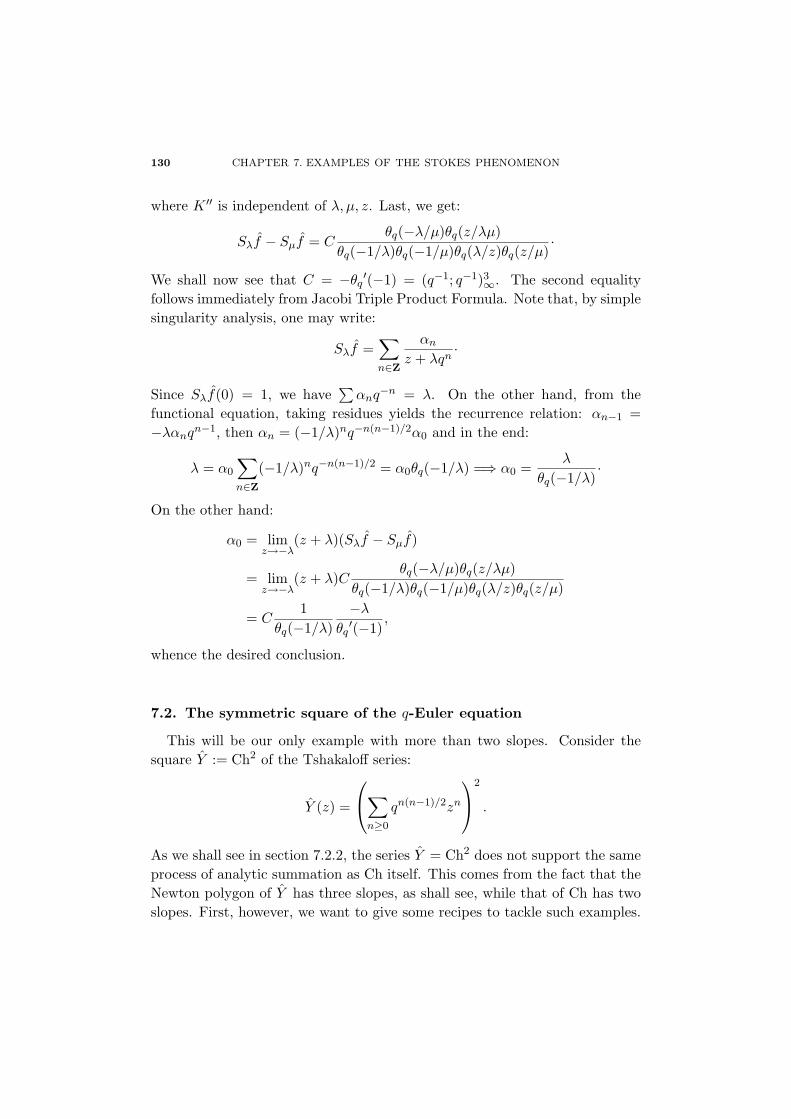
130 CHAPTER 7. EXAMPLES OF THE STOKES PHENOMENON
where K ′′ is independent of λ, µ, z. Last, we get:
Sλf − Sµf = Cθq(−λ/µ)θq(z/λµ)
θq(−1/λ)θq(−1/µ)θq(λ/z)θq(z/µ)·
We shall now see that C = −θq′(−1) = (q−1; q−1)3∞. The second equality
follows immediately from Jacobi Triple Product Formula. Note that, by simplesingularity analysis, one may write:
Sλf =∑n∈Z
αn
z + λqn·
Since Sλf(0) = 1, we have∑αnq
−n = λ. On the other hand, from thefunctional equation, taking residues yields the recurrence relation: αn−1 =−λαnq
n−1, then αn = (−1/λ)nq−n(n−1)/2α0 and in the end:
λ = α0
∑n∈Z
(−1/λ)nq−n(n−1)/2 = α0θq(−1/λ) =⇒ α0 =λ
θq(−1/λ)·
On the other hand:
α0 = limz→−λ
(z + λ)(Sλf − Sµf)
= limz→−λ
(z + λ)Cθq(−λ/µ)θq(z/λµ)
θq(−1/λ)θq(−1/µ)θq(λ/z)θq(z/µ)
= C1
θq(−1/λ)−λ
θq′(−1)
,
whence the desired conclusion.
7.2. The symmetric square of the q-Euler equation
This will be our only example with more than two slopes. Consider thesquare Y := Ch2 of the Tshakaloff series:
Y (z) =
∑n≥0
qn(n−1)/2zn
2
.
As we shall see in section 7.2.2, the series Y = Ch2 does not support the sameprocess of analytic summation as Ch itself. This comes from the fact that theNewton polygon of Y has three slopes, as shall see, while that of Ch has twoslopes. First, however, we want to give some recipes to tackle such examples.

7.2. THE SYMMETRIC SQUARE OF THE q-EULER EQUATION 131
7.2.1. Algebraic aspects. — Remember that the equation f = 1 + zσqf
satisfied by Ch is nothing but the cohomological equation for(
1 −10 z
).
7.2.1.1. Newton polygon of a symmetric square. — To find the equationsatisfied by a product of two functions, one uses the tensor product of twosystems or modules; for a square, one uses likewise the symmetric square.
Let M = (V,Φ) be a q-difference module and T 2M := M⊗M = (V ⊗V,Φ⊗Φ) its tensor square. The linear automorphism x⊗ y 7→ y⊗ x commutes withΦ ⊗ Φ, so that it actually defines an involutive q-difference automorphism ofM ⊗M , and a splitting:
T 2M = S2M ⊕ Λ2M.
If M has slopes µ1, . . . , µk with multiplicities r1, . . . , rk, then T 2M has slopesthe µi + µj , 1 ≤ i, j ≤ k with multiplicities the rirj . (Of course, if manysums µi +µj are equal, the corresponding multiplicities rirj should be added;the same remark will hold for the following computations.) Said otherwise,the slopes of T 2M are the 2µi, 1 ≤ i ≤ k with multiplicities the r2i ; and theµi + µj , 1 ≤ i < j ≤ k with multiplicities the 2rirj .
The repartition of these slopes (breaking of the Newton polygon) amongthe symmetric and exterior square is as follows:
– S2M has slopes the 2µi, 1 ≤ i ≤ k with multiplicities ther2i + ri
2; and
the µi + µj , 1 ≤ i < j ≤ k with multiplicities the rirj .
– Λ2M has slopes the 2µi, 1 ≤ i ≤ k with multiplicities ther2i − ri
2; and
the µi + µj , 1 ≤ i < j ≤ k with multiplicities the rirj .
If there are two slopes µ < ν, with multiplicities r, s, no confusion of sumsµi + µj can arise, and we find:
– T 2M has slopes 2µ < µ+ ν < 2ν, with multiplicities r2, 2rs, s2;
– Λ2M has the same slopes, with multiplicitiesr2 + r
2, rs,
s2 + s
2;
– Λ2M has the same slopes, with multiplicitiesr2 − r
2, rs,
s2 − s2·
We now take M0 =(a 00 bz
)and M =
(a u
0 bz
), where a, b ∈ C∗ and
u ∈ C(z). The symmetric squares admit an obvious choice of basis and
132 CHAPTER 7. EXAMPLES OF THE STOKES PHENOMENON
corresponding matrices:
N0 =
a2 0 00 abz 00 0 b2z2
and N =
a2 2au u2
0 abz ubz
0 0 b2z2
.
If F =(
1 f
0 1
)is such that F [M0] = M , then we have G[N0] = N with G
given by:
G = S2F =
1 2f f2
0 1 f
0 0 1
.
Actually, if one does not cheat, when looking for G =
1 f1 f2
0 1 f3
0 0 1
such that
G[N0] = N , one has to solve the system:
abzσqf1 = a2f1 + 2au,
b2z2σqf2 = a2f2 + 2auf3 + u2,
b2z2σqf3 = abzf3 + ubz.
Since we know from start that bzσqf = af + u, we see that f1 := 2f andf3 := f respectively solve the first and third equation; then, we find thatf2 := f2 solve the second equation.
Using the system above, we find a second order inhomogeneous equationfor f2 alone as follows:
(bzσq − a)1
2au(b2z2σq − a2)f2 = (bzσq − a) f3 + (bzσq − a)
u2
2au=⇒(
bz
σq(u)σq −
a
u
)(b2z2σq − a2)f2 = bzσq(u) + au.
We leave to the reader to find a simpler form, as well as the correspondingthird order homogeneous equation. At any rate, in the case that u ∈ C(Birkhoff-Guenther normal form) we have:
(bzσq − a) (b2z2σq − a2)f2 = bz + a.
In the particular case a = b = −u = 1 of the Tshakaloff series, we are led tothe following equation:
(62) LY = 1 + z, where L := q2z3σ2q − z(1 + z)σq + 1.

7.2. THE SYMMETRIC SQUARE OF THE q-EULER EQUATION 133
Remark 7.2.1. — We refer here to the example 6.2.3 and specialize it to thecase of the symmetric square N above. We see that, when u varies, the class ofN in H1(Eq, λ
(1))⊕H1(Eq, λ(2)) has components 2auL1(a2, ab) +ubL1(ab, b2)
and u2L2,0(a2, b2): a nice parabola.
7.2.1.2. Algebraic summation of Ch2. — The fact that F [A0] = A ⇒S2F [B0] = B is purely algebraic and stays true of the sum in direction c, sothat one gets the following sums:
ScG = S2(ScF ) =
1 2fc f2c
0 1 fc
0 0 1
.
Moreover, observing that x 7→
1 2x x2
0 1 x
0 0 1
is a morphism from C C to
GL3(C), one gets the explicit formula for the cocycle:
Sc,dG = S2(Sc,dF ) =
1 2fc,d f2c,d
0 1 fc,d
0 0 1
.
The algebraic sums fc have been described explicitly un subsection 7.1.1 wheretheir notation was Sλf , with λ = c.
7.2.2. Analytic aspects. —
7.2.2.1. The series Ch2 is not summable with one level. — Consider thesquare Y := Ch2 of the Tshakaloff series:
Y (z) =
∑n≥0
qn(n−1)/2zn
2
.
Its q-Borel transform Bq,1Y (at level 1) can be computed from the followingsimple remark:
f(z) =∑n≥0
anzn and g ∈ C[[z]]⇐⇒ Bq,1(f g) =
∑n≥0
anq−n(n−1)/2ξnBq,1g(q−nξ).
It follows that, if P (ξ) = Bq,1Y (ξ)∏
n≥0(1− q−nξ), then P is an entire functionsuch that:
(63) P (qm) = (−1)mqm(3m+1)/2(q−1; q−1)m(q−1; q−1)∞.

134 CHAPTER 7. EXAMPLES OF THE STOKES PHENOMENON
From this, we see that P has at infinity q-exponential growth of order ≥ 3.
The q-Borel transform of Y represents a meromorphic function in C with(simple) poles on qN and having at infinity in C \ qN q-exponential growth oforder exactly 2.
Thus, Y = Ch2 is not q-Borel-Laplace summable as Ch itself is. This comesfrom the fact that the Newton polygon of the former (resp. of the latter) hasthree (resp. two) slopes as we have seen. Moreover, the problem os cousin toa nonlinear problem.
7.2.2.2. Multisummability. —
Proposition 7.2.2. — Let λ, µ ∈ C∗ and let f ∈ A[λq and g ∈[µ]
q .
1. If [λ] = [µ], then fg ∈ O2[λ]([λ],λ]).
2. If [λ] 6= [µ], then, generically fg /∈ O[λ]+[µ]([λ],[µ]) ∪O[λ]+[µ]
([µ],[λ]).
Proof. — Write f = F/θλ, g = G/θµ; from theorem 5.2.8, one gets F ∈ E[λ]0
and G ∈ E[µ]0 .
If [λ] = [µ], then FG represents an analytic function near 0 in C∗, with q-Gevrey growth of null order on the q-spiral [λ] at 0 and q-Gevrey growth oforder 2 globally. To obtain the q-Gevrey growth order of its values on 2[λ]/[λ]at 0, write:
(FG)′(λq−n) = F ′(λq−n)G(λq−n) + F (λq−n)G′(λq−n),
which will provide the q-Gevrey order. Using theorem 5.4.3, we get the firststatement.For the second statement, just note that, generally, FG has null q-Gevreyorder at 0 neither on [λ], nor on [µ]; indeed, the sequences (F (µq−n)) and(G(λq−n)) have q-Gevrey order one.
Let λ, µ /∈ [1] = qZ. Write fλ, resp. fµ, the solutions of the q-Euler equationsatisfied by Ch in A[λ]
q , resp. in A[µ]q . If [λ] = [µ], from the proposition above,
one has:
(fλ)2 ∈ O2[λ]([λ],λ]),
and this is the solution provided by theorem 5.5.3 for equation (62) withΛ = 2[λ] and Λ1 = Λ2 = [λ]. However, if [λ] 6= [µ], then fλfµ is not thesolution provided by that theorem with Λ = [λ]+[µ] and Λ1,Λ2 = [λ], [µ].
7.3. FROM THE MOCK THETA FUNCTIONS TO THE q-EULER EQUATION 135
7.2.2.3. Possibility of a multisummation process. — No explicit algorithm ispresently known to yield the solution of (62) in the spirit of theorem 5.5.3with Λ = [λ] + [µ]. A multisummation algorithm does exist in a very differentsetting, due to the third author. The following result shows its similarity toclassical Borel-Laplace summation.
Theorem 7.2.3. — In (62), we have L = (zσq − 1)(z2σq − 1) and the seriesY is (1, 1/2)-summable by the following process:
f =∑n≥0
anzn Bq,1−→ ϕ :=
∑n≥0
anq−n(n−1)/2ξn
A∗q;1,1/2−→ f∗1
L∗q;1/2−→ f∗(1,1/2).
For a basic introduction to this method and explanation of the notationsabove, see [16], which contains further references to this work.
7.3. From the Mock Theta functions to the q-Euler equation
Our source here is the famous 1935 paper “The final problem: an accountof the Mock Theta Functions” by G. N. Watson, as reproduced, for instance,in [3]. On page 330 of loc. cit., seven “mock theta functions of order three”are considered. The first four are called f, φ, ψ, χ (after Ramanujan whodiscovered them); the three last are called ω, ν, ρ (after Watson who addedthem to the list). In the notation of Ramanujan and Watson, the uniquevariable of these analytic functions is written q (this tradition goes back toJacobi) and it is assumed there that 0 < |q| < 1.
In [59], a new variable x is added (this tradition goes back to Euler) andone puts:
s(α, β; q, x) :=∑n≥0
anxn,
where:
an :=qn2(
qα ,
qβ ; q)
n
(1αβ
)n
=(α, β; q)∞
(αq−n, βq−n; q)∞q−n
=qn2
(α− q) · · · (α− qn)(β − q) · · · (β − qn)·

136 CHAPTER 7. EXAMPLES OF THE STOKES PHENOMENON
Note for further use that the second formula makes sense for all n ∈ Z andallows one to define another series:
F (α, β; q, x) :=∑n∈Z
anxn,
so that F (α, β; q, x) = s(α, β; q, x) +G(α, β; q, x), where:
G(α, β; q, x) =∑n<0
anxn =
∑n≥0
(α, β; q)n(q/x)n.
The formula giving s(α, β; q, x) subsumes all seven mock theta functions, whichcan be respectively recovered by setting (α, β, x) to be one of the following:(−1,−1, 1), (i,−i, 1), (
√q,−√q, 1), (j, j2,−q), (1/q, 1/q, 1), (i/
√q,−i/
√q, 1)
and (−j/q,−j2/q, 1). (Note that in all cases, among other multiplicativerelations, α and β map to torsion points of Eq.)
In the following, which is intended to motivate the study of the Stokesphenomenon, we follow recent work by the third author [59], skipping mostof the proofs. In 7.3.1 and 7.3.2, we use the conventions of loc. cit. and usethe theta function:
θ(x; q) :=∑n∈Z
qn(n−1)/2xn = (q,−x,−q/x; q)∞ = θq−1(q−1x).
(See the general notations in section 1.3.) In 7.3.3, we shall return to thegeneral conventions of the present paper.
7.3.1. Functional equation for s(α, β; q, z). — From the recurrence rela-tion (α− qn+1)(β− qn+1)an+1 = q2n+1an, one deduces that s, as a function ofx, is solution of the second order non homogeneous q-difference equation:
(64)((σq − α)(σq − β)− qxσ2
q
)s = (1− α)(1− β).
The recurrence relation actually remains valid for all n ∈ Z, which impliesthat F is solution of the corresponding homogeneous equation:
(65)((σq − α)(σq − β)− qxσ2
q
)F = 0.
This, in turn, entails that −G = s−F is a solution defined at infinity of (64).
We shall assume now that α, β 6= 0 and that β/α 6∈ qZ. One checks easilythat the equation (65) is fuchsian at 0 with exponents α, β (see for instance[44]). Likewise, taking in account the general conventions of this paper (i.e.using the dilatation factor q−1 in order to have a modulus> 1), we see that (65)

7.3. FROM THE MOCK THETA FUNCTIONS TO THE q-EULER EQUATION 137
is pure isoclinic at infinity, with slope −1/2; this will explain the appearanceof θ(−, q2) in the following formulas. We define:
M(α, β; q, x) :=(q
α,q
β; q)∞F (α, β; q, x).
This is another solution of (65), with more symetries. It admits the followingexpansions:
M(α, β; q, x) = θ(qαβx; q2)Uα/β(x)− q
αθ(αβx; q2)Vα/β(x)
= θ(qx/αβ; q2)Uα/β(1/x)− q
αθ(q2x/αβ; q2)Vα/β(1/x),
with the following definitions:
Uλ(x) :=∑m≥0
qm2S2m(−q−2mλ; q)(qx/λ)m,
Vλ(x) :=∑m≥0
qm(m+1)S2m+1(−q−2m−1λ; q)(qx/λ)m,
Sn(x; q) :=n∑
k=0
qk2
(q; q)k(q; q)n−k(−x)k.
(The Sn are the Stieltjes-Wiegert polynomials.)
Remark 7.3.1. — The parameter λ := α/β is linked to monodromy. Indeed,
the local Galois group of (65) at 0 is the set of matrices(γ(α) 0
0 γ(β)
), where
γ runs through the group endomorphisms of C∗ that send q to 1; and thelocal monodromy group is the rank 2 free abelian subgroup with generatorscorresponding to two particular choices of γ described in [45].
7.3.2. Back to the the Mock Theta function. — We can for instancestudy φ, ψ, ν, ρ by setting x = 1 in s(α, β; q, x). (The function χ involvesx = −q and f, ω will not comply the condition β/α 6∈ qZ: in [59], their studyis distinct, though similar.) Up to the knowledge of standard q-functions, oneis reduced to the study of:
U(λ) := Uλ(1) and V (λ) := Vλ(1).
138 CHAPTER 7. EXAMPLES OF THE STOKES PHENOMENON
These are solutions of the q-difference equations:
U(qλ)− λU(λ/q) = (1− λ)θ(qλ; q2)(q, q; q)∞
,
V (qλ)− qλV (λ/q) = (1− λ)θ(λ/q; q2)(q, q; q)∞
·
Upon setting:
U(λ) =:θ(λ; q2)
(q, q; q)∞Y (λ) and V (λ) =:
θ(λ/q; q2)(q, q; q)∞
Z(λ),
we find that both Y and Z are solutions of the q-difference equation:
X(qλ)− λ2
qX(λ/q) = 1− λ.
7.3.3. Back to the q-Euler equation. — To fit this equation with theconvention of this paper, we shall put z := λ, f(z) := X(qλ) and take q−2
as the new dilatation coefficient, that we shall denote by q, so that |q| > 1indeed. Our equation becomes:
√qz2σqf − f = z − 1.
(We have implicitly chosen a square root√q.) There are four pathes of attack.
The most poweful involves the summation techniques of chapter 5 and it isthe one used in [59]. We show the other three as an easy application exercise.
7.3.3.1. q-Borel transformation. — Following 3.1.1, we put Z := z2, Q := q2
and f(z) = g(Z) + zh(Z), so that:
√qZσQg − g = −1 and q
√qZσQh− h = 1.
The end of the computation, i.e. that of the invariants (BQ,1)(−1)(√q) and
(BQ,1)(1)(q√q), is left to the reader.
7.3.3.2. Birkhoff-Guenther normal form. — According to section 3.3, we seethat our equation is already in Birkhoff-Guenther normal form. Actually, it is
the equation for f such that(
1 f
0 1
)is an isomorphism from
(1 00√qz2
)to(
1 z − 10√qz2
).
7.4. FROM CLASS NUMBERS OF QUADRATIC FORMS TO THE q-EULER EQUATION139
7.3.3.3. Privileged cocycles. — There is here an obvious isomorphism ofΛI(M0) with the vector bundle F1/
√qz2 (cf. 3.1.1). (More generally, if
A0 =(a 00 bzδ
), then ΛI(M0) ' Fa/bzδ .) The privileged cocycles of 6.1 are
best obtained by the elementary approach of [46] as follows. We look for asolution fc =
g
θ2q,c
with g holomorphic over C∗. The corresponding equation
is√qc2σqg − g = (z − 1)θ2
q,c. Writing θq2 =:
∑τnz
n, we see that:
fc =1θ2q,c
∑n∈Z
(τn−1c− τn)c−n
√qc2qn − 1
zn.
This is the only solution with poles only on [−c; q] and at most double. Itmakes sense only for
√qc2 6∈ qZ, which prohibits four values c ∈ Eq. The
components of the Stokes cocycle are the (fc − fd).
7.4. From class numbers of quadratic forms to the q-Euler equation
This topic is related to a paper of Mordell [30] and to recent work [58] bythe third author. We follow their notations, except for the use of the letter q,and also for the dependency on the modular parameter ω, which we do notalways make explicit.
We shall have here use for the classical theta functions, defined for x ∈ Cand =(ω) > 0:
θ0,1(x) = θ0,1(x, ω) :=∑n∈Z
(−1)neiπ(n2ω+2nx),
θ1,1(x) = θ1,1(x, ω) :=1i
∑m odd
(−1)(m−1)/2eiπ(m2ω/4+mx),
= eiπ(ω/4+x−1/2)∑n∈Z
(−1)neiπ(n(n+1)ω+2nx).
We shall set q := e−2iπω (so that indeed |q| > 1) and z := e2iπx. The abovetheta functions are related to θq through the formulas:
θ0,1(x, ω) = θq(−√qz),
θ1,1(x, ω) =√z
iq1/8θq(−z).
(Thus, the latter is multivalued as a function of z.)

140 CHAPTER 7. EXAMPLES OF THE STOKES PHENOMENON
7.4.1. The generating series for the class numbers. — Consider thequadratic forms ax2 +2hxy+by2, with a, b, h ∈ Z, a, b not both even (“unevenforms”), and D := ab− h2 > 0, up to the usual equivalence. For any D ∈ N∗,write F (D) the (finite) number of classes of such forms.
Theorem 7.4.1 (Mordell, 1916)). — Let f0,1(x) = f0,1(x, ω) the uniqueentire function solution of the system:
f0,1(x+ 1) = f0,1(x),
f0,1(x+ ω) + f0,1(x) = θ0,1(x).
Then, for =(ω) > 0: ∑n∈N∗
F (n)eiπnω =i
4πf ′0,1(0)θ0,1(0)
·
If one now defines G0,1(z) :=f0,1(x)θ0,1(x)
(which does make sense, since the right
hand side is 1-periodic), one falls upon the familiar q-difference equation:
(√qzσq − 1)G0,1 =
√qz.
We leave it as an exercise for the reader to characterize G0,1 as the uniquesolution complying some polar conditions.
7.4.2. Modular relations. — In order to obtain modular and asymptoticproperties for the generating series of theorem 7.4.1, Mordell generalized hisresults in 1933. We extract the part illustrating our point. Mordell sets:
f(x) = f(x, ω) :=1i
∑m odd
(−1)(m−1)/2eiπ(m2ω/4+mx)
1 + eiπωm·
This the unique entire function solution of the system:f(x+ 1) + f(x) = 0,
f(x+ ω) + f(x) = θ1,1(x).
The interest for Mordell is the (quasi-)modular relation:
f(x, ω)− iωf(x/ω,−1/ω) =
1iθ1,1(x, ω)
∫ +∞
−∞
eiπωt2−2πtx
e2πt − 1dt.
(The path of integration is R except that one avoids 0 by below.) The interest
for us is that one can put G(z) :=f(x)θ1,1(x)
(the right hand side is 1-periodic),
7.4. FROM CLASS NUMBERS OF QUADRATIC FORMS TO THE q-EULER EQUATION141
and get the same equation as before:
(√qzσq − 1)G =
√qz.
This is used in [58] to generalize Mordell results: the fundamental idea is tocompare two summations of the solutions, one along the lines of the presentpaper, the other along different lines previously developped by C. Zhang.
7.4.3. Related other examples. — Mordell also mentions that the fol-lowing formula of Hardy and Ramanujan:
1√−iω
∫ +∞
−∞
e−iπ(t−ix)2/ω
coshπtdt =
∫ +∞
−∞
eiπωt2−2πtx
coshπtdt
can be proved along similar lines, by noting that both sides are entire solutionsof the system: Φ(x− 1) + Φ(x) =
2eiπ(x−1/2)2/ω
√−iω
,
Φ(x+ ω) + eiπ(2x+ω)Φ(x) = 2eiπ(3ω/4+x)
and that the latter admits only one such solution.


BIBLIOGRAPHY
[1] Yves Andre. Differentielles non commutatives et theorie de Galoisdifferentielles ou aux differences. Ann. Sci. c. Norm. Supr. (4), 34(5):685–739, 2001.
[2] D.G. Babbitt and V.S. Varadarajan. Local moduli for meromorphic differ-ential equations. Centre National de la Recherche Scientifique. Asterisque,169-170. Paris: Societe Mathematique de France., 1989.
[3] Bruce C. (ed.) Berndt and Robert A. (ed.) Rankin. Ramanujan: essaysand surveys. History of Mathematics (Providence) 22. Providence, RI:American Mathematical Society (AMS); London: London MathematicalSociety., 2001.
[4] Daniel Bertrand. Extensions panachees et 2-extensions. manuscrit nonpublie, 1999.
[5] Daniel Bertrand. Extensions panachees et dualite. Prepublications del’Institut Mathematique de Jussieu, (287), 2001.
[6] Jean-Paul Bezivin. Sur les equations fonctionnelles aux q-differences. Ae-quationes Math., 43(2-3):159–176, 1992.
[7] George D. Birkhoff. Singular points of ordinary linear differential equa-tions. Trans. Amer. Math. Soc., 10:436–470, 1909.
[8] George D. Birkhoff. The generalized riemann problem for linear differen-tial equations and the allied problems for linear difference and q-differenceequations. Proc. Amer. Acad., 49:521–568, 1913.
[9] George D. Birkhoff and Paul E. Guenther. Note on a canonical form forthe linear q-difference system. Proc. Nat. Acad. Sci. U. S. A., 27:218–222,1941.

144 BIBLIOGRAPHY
[10] N. Bourbaki. Elements de mathematiques. Algebre. Chapitre 10: Algebrehomologique. Paris etc.: Masson. VII, 216 p. , 1980.
[11] B.L.J. Braaksma, B.F. Faber, and G.K. Immink. Summation of formalsolutions of a class of linear difference equations. Pac. J. Math., 195(1):35–65, 2000.
[12] Henri Cartan and Samuel Eilenberg. Homological algebra. PrincetonMathematical Series, 19. Princeton, New Jersey: Princeton UniversityPress XV. , 1956.
[13] Richard M. Cohn. Difference algebra. Interscience Publishers John Wiley& Sons, New York-London-Sydney, 1965.
[14] Lucia Di Vizio. Arithmetic theory of q-difference equations: the q-analogue of Grothendieck-Katz’s conjecture on p-curvatures. Invent.Math., 150(3):517–578, 2002.
[15] Lucia Di Vizio. Local analytic classification of q-difference equations with|q| = 1. J. Noncommut. Geom., 3(1):125–149, 2009.
[16] Lucia Di Vizio, Jean-Pierre Ramis, Jacques Sauloy, and ChangguiZhang. Equations aux q-differences. (French) [q-difference equations],.Gaz. Math., (96):20–49, 2003.
[17] Lucia Di Vizio and Changgui Zhang. On q-summation and confluence.Ann. Inst. Fourier, 59(1):347–392, 2009.
[18] Charles H. Franke. Picard-Vessiot theory of linear homogeneous differenceequations. Trans. Amer. Math. Soc., 108:491–515, 1963.
[19] Jean Frenkel. Cohomologie non abelienne et espaces fibres. Bull. Soc.Math. Fr., 85:135–220, 1957.
[20] S.I. Gelfand and Yu.I. Manin. Methods of homological algebra. Transl.from the Russian. 2nd ed. Springer Monographs in Mathematics. Berlin:Springer., 2003.
[21] A. Grothendieck. Modeles de Neron et monodromie. (Avec un appendicepar M. Raynaud.). Sem. Geom. algebrique Bois-Marie 1967-1969, SGA 7I. No.9, Lect. Notes Math. 288, 313-523 (1972)., 1972.
[22] Gertrude K. Immink. On meromorphic equivalence of linear differenceoperators. Ann. Inst. Fourier, 40(3):683–699, 1990.
[23] Sauloy Jacques. Classification des modules aux differences filtres iso-gradues. Article soumis, 2009.

BIBLIOGRAPHY 145
[24] Bernard Malgrange. Le theoreme de preparation en geometriedifferentiable. Topologie Differ., Semin. H. Cartan 15 (1962/63), No.11,14 p. (1964), No.12, 9 p. (1964), No.13, 12 p. (1964), No.22, 8 p. (1964).,1964.
[25] Bernard Malgrange. Ideals of differentiable functions. (Tata Institute ofFundamental Research Studies in Mathematics. Vol. 3). London: OxfordUniversity Press, 106 p. , 1966.
[26] Bernard Malgrange. Sur les points singuliers des equations differentielles.L’enseignement Mathematique II. Ser., 20:147–176, 1974.
[27] Fabienne Marotte and Changgui Zhang. Multisummability of formalpower series solutions of linear analytic q-difference equations. (Multi-sommabilite des series entieres solutions formelles d’une equation auxq-differences lineaire analytique.). Ann. Inst. Fourier, 50(6):1859–1890,2000.
[28] Jean Martinet and Jean-Pierre Ramis. Problemes de modules pour desequations differentielles non lineaires du premier ordre. Publ. Math., Inst.Hautes tud. Sci., 55:63–164, 1982.
[29] Jose Luis Martins. Lemme de Watson en dimension suprieure et applica-tion la sommation des solutions des D-modules holonomes. PhD thesis,Universit Paul Sabatier, Toulouse, 2002.
[30] L.J. Mordell. The definite integral∫∞−∞
eax2+bx
ecx+d dx and the analytic theoryof numbers. Acta Math., 61:323–360, 1933.
[31] Oystein Ore. Theory of non-commutative polynomials. Annals of Math.,34(2):480–508, 1933.
[32] J.-P. Ramis and J. Sauloy. The q-analogue of the wild fundamental group.I. In Algebraic, analytic and geometric aspects of complex differentialequations and their deformations. Painleve hierarchies, RIMS KokyurokuBessatsu, B2, pages 167–193. Res. Inst. Math. Sci. (RIMS), Kyoto, 2007.
[33] Jean-Pierre Ramis. About the growth of entire functions solutions of lin-ear algebraic q-difference equations. Ann. Fac. Sci. Toulouse Math. (6),1(1):53–94, 1992.
[34] Jean-Pierre Ramis. Divergent series and asymptotic theories. (Series di-vergentes et theories asymptotiques. Suppl. au Bulletin de la SMF.) Bul-letin de la Societe Mathematique de France 121. Panoramas et Syntheses.v. 121. Paris: Societe Mathematique de France., 1993.

146 BIBLIOGRAPHY
[35] Jean-Pierre Ramis and Sauloy Jacques. The q-analogue of the wild fun-damental group. III. In preparation, 2009.
[36] Jean-Pierre Ramis and Jacques Sauloy. The q-analogue of the wild funda-mental group. II. In Differential Equations and Singularities, 60th yearsof J.M. Aroca, volume 323. Societe Mathematique de France, 2009.
[37] Jean-Pierre Ramis, Jacques Sauloy, and Changgui Zhang. La variete desclasses analytiques d’equations aux q-differences dans une classe formelle.C. R. Math. Acad. Sci. Paris, 338(4):277–280, 2004.
[38] Jean-Pierre Ramis, Jacques Sauloy, and Changgui Zhang. Dveloppementasymptotique et sommabilit des solutions des quations linaires aux q-diffrences. C. R. Math. Acad. Sci. Paris, 342(7):515–518, 2006.
[39] Jean-Pierre Ramis and Changgui Zhang. q-Gevrey asymptotic expansionand Jacobi theta function. (Developpement asymptotique q-Gevrey etfonction theta de Jacobi.). C. R., Math., Acad. Sci. Paris, 335(11):899–902, 2002.
[40] Julien Roques. Rational classification and confluence of regular singulardifference systems. (Classification rationnelle et confluence des systemesaux differences singuliers reguliers.). Ann. Inst. Fourier, 56(6):1663–1699,2006.
[41] Julien Roques. Sur les quations aux (q-) diffrences. PhD thesis, UniversitPaul Sabatier, Toulouse, 2007.
[42] Claude Sabbah. Introduction to algebraic theory of linear systems of dif-ferential equations. Maisonobe, Philippe (ed.) et al., D-modules coherentset holonomes. Cours d’ete du CIMPA ’Elements de la theorie des systemesdifferentiels’, aout et septembre 1990, Nice, France. Paris: Hermann.Trav. Cours. 45, 1-80 (1993)., 1993.
[43] J. Sauloy. Equations aux q-differences et fibres vectoriels sur une courbeelliptique. In Differential Equations and Singularities, 60th years of J.M.Aroca, volume 323. Societe Mathematique de France, 2009.
[44] Jacques Sauloy. Systemes aux q-differences singuliers reguliers: classifica-tion, matrice de connexion et monodromie. Ann. Inst. Fourier (Grenoble),50(4):1021–1071, 2000.
[45] Jacques Sauloy. Galois theory of Fuchsian q-difference equations. Ann.Sci. Ecole Norm. Sup. (4), 36(6):925–968 (2004), 2003.

BIBLIOGRAPHY 147
[46] Jacques Sauloy. Algebraic construction of the Stokes sheaf for irregu-lar linear q-difference equations. Asterisque, 296:227–251, 2004. Analysecomplexe, systemes dynamiques, sommabilite des series divergentes ettheories galoisiennes. I.
[47] Jacques Sauloy. La filtration canonique par les pentes d’un module aux q-differences et le gradue associe. Ann. Inst. Fourier (Grenoble), 54(1):181–210, 2004.
[48] Jacques Sauloy. The geometry of the space of isoformal analytic classesof q-difference equations. in preparation, 2010.
[49] V. Tarasov and A. Varchenko. Geometry of q-hypergeometric functions,quantum affine algebras and elliptic quantum groups. Asterisque. 246.Paris: Societe Mathematique de France, 1997.
[50] W. J. Trjitzinsky. Analytic theory of linear q-difference equations. ActaMath., 61:1–38, 1933.
[51] Marius van der Put and Marc Reversat. Galois theory of q-differenceequations. Ann. Fac. Sci. Toulouse Math. (6), 16(3):665–718, 2007.
[52] Marius van der Put and Michael F. Singer. Galois theory of differenceequations, volume 1666 of Lecture Notes in Mathematics. Springer-Verlag,Berlin, 1997.
[53] Changgui Zhang. Developpements asymptotiques q-Gevrey et series Gq-sommables. (q-Gevrey asymptotic expansions and Gq-summable series.).Ann. Inst. Fourier, 49(1):227–261, 1999.
[54] Changgui Zhang. A discrete summation for linear q-difference equationswith analytic coefficients: General theory and examples. (Une sommationdiscrete pour des equations aux q-differences lineaires et a coefficientsanalytiques: Theorie generale et exemples.). Braaksma, B. L. J. (ed.) etal., Differential equations and the Stokes phenomenon. Proceedings of theconference, Groningen, Netherlands, May 28–30, 2001. Singapore: WorldScientific. 309-329 (2002)., 2002.
[55] Changgui Zhang. Remarks on some basic hypergeometric series. Ismail,Mourad E. H. (ed.) and Koelink, Erik (ed.), Theory and applications ofspecial functions. A volume dedicated to Mizan Rahman. Papers fromthe Special Session of the American Mathematical Society annual meet-ing held in Baltimore, MD, USA, January 15–18, 2003. Developments inMathematics 13. New York, NY: Springer., 2005.

148 BIBLIOGRAPHY
[56] Changgui Zhang. Asymptotic and meromorphic solutions of q-differenceequations. (Solutions asymptotiques et meromorphes d’equations auxq-differences.). Delabaere, Eric (ed.) et al., Theories asymptotiqueset equations de Painleve. Paris: Societe Mathematique de France.Seminaires et Congres 14, 341-356 (2006)., 2006.
[57] Changgui Zhang. Confluent basic hypergeometric series. preprint (alsosee [55]), 2010.
[58] Changgui Zhang. On mock theta functions. in preparation, 2010.
[59] Changgui Zhang, Luo Z., and Zhou S. On summability of formal solutionsto a cauchy problem and a generalisation of mordell’s theorem. submitted,2010.


![Stochastic isentropic Euler equationsmath.univ-lyon1.fr/~vovelle/BerthelinVovelle.pdf · Bauzet, Vallet, Wittbold [BVW12], kinetic formulation (Debussche, Vovelle [DV10,DV], the more](https://img.dokumen.tips/doc/110x75/5e92d39ae5a82f7a710084f5/stochastic-isentropic-euler-vovelleberthelinvovellepdf-bauzet-vallet-wittbold.jpg)

![PEP Web - The Analytic Third: Working with Intersubjective ... … · analytic third'. This third subjectivity, the intersubjective analytic third Green's [1975] 'analytic object'),](https://img.dokumen.tips/doc/110x75/6099619e2d4b51336024f694/pep-web-the-analytic-third-working-with-intersubjective-analytic-third.jpg)