Loan Sales and Relationship Banking

THE JOURNAL OF FINANCE • VOL. LXIII, NO. 3 • JUNE 2008

Loan Sales and Relationship Banking

CHRISTINE A. PARLOUR and GUILLAUME PLANTIN∗

ABSTRACT

Firms raise money from banks and the bond market. Banks sell loans in a secondarymarket to recycle their funds or to trade on private information. Liquidity in the loanmarket depends on the relative likelihood of each motive for trade and affects firms’optimal financial structure. The endogenous degree of liquidity is not always sociallyoptimal: There is excessive trade in highly rated names, and insufficient liquidity inriskier bonds. We provide testable implications for prices and quantities in primaryand secondary loan markets, and bond markets. Further, we posit that risk-basedcapital requirements may be socially desirable.

THE TERM “COLLATERALIZED LOAN OBLIGATIONS” (CLOs) was coined in 1989, whencorporate loans were first used as collateral in Collateralized Debt Obligations(CDOs).1 Since then, the growth in loan sales has been enormous. According toLucas et al. (2006), $1.1 trillion of CDOs were outstanding as of 2005, and 50%of their collateral was comprised of loans. In addition to pooled securities, banksalso trade first loss positions on single names through direct sales of individualloans. In the United States, loan sales have grown from $8 billion in 1991 to$154.8 billion by 2004.2 If a bank securitizes or sells a loan that it originated,it is buying insurance on credit events over which it has either more control ormore information than the buyer.

In the face of this informational friction, why did the secondary market forcorporate loans develop in the 1990s? What effect has this had on relationshipbanking? In this paper, we characterize when a liquid secondary market forloans arises, when a liquid secondary loan market is socially desirable, and weprovide testable predictions on the effect of the emergence of this market onprices and quantities in bond and primary loan markets. Our predictions arebased on both changes in the parameters that lead to higher loan liquidity andchanges in the contracts that are written between banks and firms given thishigher liquidity.

∗Parlour is from the Haas School, UC Berkeley, and Plantin is from the London Business School.We have benefitted from helpful comments by Viral Acharya, Doug Diamond, Denis Gromb, RupertCox, Martin Ruckes, an anonymous referee, and the editor Rob Stambaugh. In addition, we thankseminar participants at Baruch, IHS (Vienna), the Federal Reserve Bank of New York, Centerfor Financial Studies Credit Risk Conference (Frankfurt), the London School of Economics, Yale,Stanford, the Western Finance Association, Berkeley, and the Federal Reserve Bank of Richmond.A previous version of this paper was entitled “Credit Risk Transfer.”

1 This is reported in Lucas, Goodman, and Fabozzi (2006).2 This figure is reported in Drucker and Puri (2006).

1291

1292 The Journal of Finance

Two views on the rise of active credit risk management by banks have beenproposed. First, more liquid bank assets make asset-liability management eas-ier. Banks can quickly redeploy capital to more profitable business opportu-nities and are more resilient to negative shocks, as in Greenspan (2004) andSchuermann (2004). Following this view, active secondary loan markets aresocially beneficial. Second, and more perniciously, banks can now unbundlebalance sheet management from borrower relationship management. This mayreduce banks’ incentives to monitor and foster a relationship with the borrower,and ultimately create a shift from relationship banking to transaction-orientedbanking (a view espoused by Effenberger (2003), Kiff and Morrow (2000), andRule (2001) among others). If relationship banking adds value, then loan liq-uidity may be harmful. We demonstrate that with endogenous loan liquidity,either of these cases can obtain.

In our stylized model, a firm has a risky, positive-NPV long-term project thatcan be financed with the firm’s own equity or from two outside sources, namely,a bank and the bond market. The optimal financing mix maximizes the firm’sreturn on equity subject to the resolution of a moral hazard problem: The firmmay shirk, which reduces the project’s success probability. A bank adds value,because it can reduce a firm’s incentive to shirk. However, through monitoring,banks gain private information about the project’s success. After monitoring,a bank may receive an attractive outside investment opportunity and wish toredeploy its funds. An active secondary market gives the bank the flexibilityto recycle capital. However, a liquid market may also reduce a bank’s incentiveto monitor as it could also sell nonperforming loans. The impact of an activesecondary loan market on banks and firms depends on this trade-off between alower monitoring incentive and the increased flexibility offered by this market.

In our model, banks differ from the bond market in three ways. First, banksare better able to monitor the firm than the bond market. This could be becausebondholders are typically dispersed and thus individually have a smaller in-centive to monitor. Second, while monitoring, the bank learns about the successor failure of the project. Thus, in our model monitoring both resolves the moralhazard problem and generates proprietary information for the bank. Many ofour results are driven by these joint assumptions. Finally, we posit that bankshave a preference for liquid assets.

The assumption that lending generates proprietary information about theborrower is common in the banking literature (Rajan (1992)), and well docu-mented empirically (e.g., Lummer and McConnell (1989)). In our setting, how-ever, the acquisition of material information is an ineluctable but adverse con-sequence of monitoring.3 Thus, there is a tension between monitoring and thetradeability of the bank’s risks, which in turn makes monitoring costly if thebank values flexibility. This assumption captures the intuition that an impor-tant part of the information that a bank acquires in order to monitor the firmalso helps to predict the firm’s future performance, and cannot be credibly com-municated to outsiders. Examples of such information include the assessment

3 This assumption follows Breton (2003).

Loan Sales and Relationship Banking 1293

of the top management’s character, or an understanding of the allocation ofreal authority within the firm. This type of information is essentially soft, andacquired by the loan officer through ongoing personal interaction with the topmanagement. Other examples of information that is necessary for monitor-ing purposes but cannot be made publicly available include the trade secretsthat generate a project’s value and whose disclosure would erode competitiveadvantage.

Liquidity is valuable in our model because a loan on its balance sheet mayprevent a bank from exploiting private redeployment opportunities, either dueto insufficient liquidity or binding capital adequacy requirements. The sec-ondary loan market is only liquid if adverse selection risk is sufficiently low.A bank that has monitored a firm knows if the project will succeed or fail.Thus, investors do not know if the bank is shedding risk because of outsideinvestment opportunities, or because of inside information. If the adverse se-lection problem is too severe, trading in the secondary market breaks downas in Akerlof (1970) and all loans are illiquid. However, if the probability thatthe bank is selling its loan for private motives is sufficiently high then thereis pooling and the market is liquid. Possible inside trading by banks in thesecondary credit market is reported in the popular press as a concern amongpractitioners.4 Altman, Amar, and Saunders (2004) find that returns in the sec-ondary market for loans lead bond and stock returns around important creditevents.

Although the rise of an active loan market is socially efficient ex post, it maynot be socially desirable ex ante. A liquid market has two opposite effects on thecost of bank debt. On one hand, interest rates on loans are smaller because thebank no longer charges a liquidity premium. On the other hand, the incentivecompatible stake of the bank in the project increases, because the ability tobenefit from inside trading reduces the bank’s incentives to monitor ex ante. Insum, firms must borrow more from banks, albeit at a lower price, if there is aliquid loan market.

Our model has a number of testable implications. We first observe thatthe credit spread in the secondary loan market is not the unconditionalprobability that the reference entity will default: rather, it is the probabil-ity of default conditional on a bank’s willingness to sell. The unconditionaland conditional probabilities differ systematically with a firm’s default prob-ability, thereby generating an observed liquidity premium in the secondarymarket.

The rest of our testable implications relate prices and quantities in bond andprimary loan markets after a secondary loan market has arisen. We posit thatthe secondary market arose because of regulatory changes in the early 1990s.First, we predict that secondary trading volume should be larger for high-gradenames. Second, a larger trading volume implies that bank loans and privatelyplaced debt crowd out public bonds in firms’ total debt issuances. Third, a liquidloan market is efficient, namely, increases firms’ total debt capacity, only if the

4 See The Economist, “Pass the Parcel”, Jan. 16, 2003.


firm is not too highly rated. Fourth, as the secondary market arises due to areal shock to bank capital, all bank loans are affected and the prices becomemore sensitive to credit risk for all ratings.

Gorton and Pennacchi (1995) and Pennacchi (1988) study incentive compati-ble loan sales contracts that provide the bank with incentives to keep monitor-ing the borrower after having sold the loan. Loan liquidity is always desirableand second-best efficient in their setups. This paper focuses instead on the im-pact of such ex post efficient sales on the incentives of the bank to monitor theborrower ex ante. We show that liquidity may rise in the secondary loan marketeven though this is ex ante inefficient.

Our basic model of moral hazard is adapted from Holmstrom and Tirole(1997). Our work is also related to that of Maug (1998), and Kahn and Winton(1998). We defer a discussion of these papers to Section V. In nonbanking con-texts, Aghion, Bolton, and Tirole (2004), and Faure-Grimaud and Gromb (2003)develop models in which an impatient agent markets claims to her future out-put. The informational efficiency of the market is an important incentive devicefor the agent. By contrast, in our model liquidity makes incentives more dif-ficult to enforce because in a liquid market, the bank trades with uninformedagents.

We provide a description of the model in Section I, followed by a characteri-zation of the optimal contracts in Section II. We establish the conditions underwhich a liquid loan market is socially efficient and those under which it is liquidin Section III. The cross-sectional implications of our model are presented inSection IV. We discuss robustness and extensions in our conclusion, Section V.All proofs appear in the Appendix.

I. Model

In an economy with three dates, t = 0, 1, and 2, there are three classes ofagents: a firm, a bank, and a large pool of competitive investors. All agents arerisk neutral and are protected by limited liability.5 Neither the investors northe firm discount future cash flows.

The firm owns the rights to a two-period constant returns to scale project.Every dollar invested in the project at t = 0 has a random date 2 payoff of R withprobability p, or zero with probability 1 − p. The firm also has initial equity ornet assets, A. In addition to investing its own assets in the project, the firm cansolicit additional funds from the bank and the outside investors. To do so, thefirm offers each group a contract at t = 0. The firm’s objective is to maximizeexpected return on equity.

This simple specification allows us to abstract from security design issuesin order to focus on prices and volumes in bond and loan markets. A largeliterature explains the benefits from pooling risks in security issuances plagued

5 Specifically, we assume that all contractible payments are bounded below by a finite amountthat we normalize to zero.


by informational asymmetry.6 We discuss the implications of a more generalstochastic structure in Section V.

Some actions taken by the firm are not observable to outside investors. Inparticular, after raising outside funds, the firm may “shirk” and derive a privatebenefit BF per dollar invested at t = 1. In this case, the project fails and paysoff zero at date 2. This moral hazard problem means that financial structurematters.

Active monitoring at t = 0 by the bank reduces the firm’s private benefitper unit of investment from shirking to bF < BF. Monitoring is costly for thebank as it loses a private benefit BB per dollar of the project associated withnot monitoring.7 An additional consequence of monitoring is that, through itsrelationship with the firm, the bank acquires private information about theproject. For simplicity, we assume that private information is perfect: If thebank monitors, it learns the project’s outcome at date 1.

Our main departure from Holmstrom and Tirole (1997) is the assumptionthat the bank maximizes a utility function with a stochastic discount factor. Att = 0, the utility of a bank is

U B(c0, c̃1, c̃2) = E(c0 + δ1c̃1 + δ1δ̃2c̃2),

where δ1 ∈ (0, 1) and δ̃2 is a two-point random variable whose realization atdate 1 is

δ̃2 ={

δ ∈ (0, 1) with probability q

1 with probability 1 − q.

The bank’s realization of δ̃2 at date 1 is private information.8

The stochastic discount factor δ̃2 proxies for unanticipated changes in the op-portunity cost of carrying outstanding loans. More precisely, it captures the ideathat the bank receives new private opportunities to invest with other borrowersor nonlending business, but may be unable to seize them if it has insufficientliquid assets or binding capital adequacy ratios. We discuss the interpretationof δ in more detail below.

After the bank has received her discount factor shock and learned the realiza-tion of the project, we assume that she can offer new contracts to the investors.9

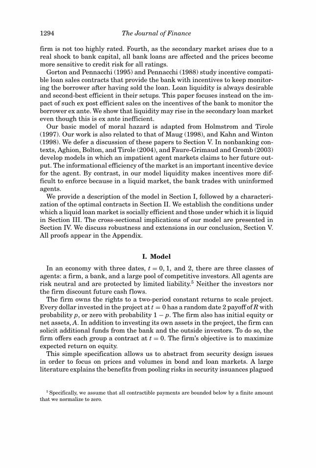
The timeline is presented in Figure 1.The assumption that the bank only monitors during the first period is for sim-

plicity. An additional moral hazard problem during period 2 would complicate

6 DeMarzo (2005) represents a recent contribution.7 Alternatively, one could model the bank as incurring a private monitoring cost. The current

formulation is the simplest one that ensures all constraints bind at the optimum.8 We assume that the realization of a bank’s discount factor at t = 1 takes on two possible values

for simplicity. The qualitative results go through if the bank’s outside opportunities are drawn froma known continuous distribution.

9 That the bank has all the bargaining power at time 1 simplifies the derivation of the optimalcontracts, but is not crucial to our results. The key driver of the results is that the bank acquiresproprietary information through monitoring.


Figure 1. Sequence of events.

the analysis without offering any further insights. We note in passing that thisfirst period need not be long. “Monitoring” may mean, for example, restrictingthe initial choice of assets made by the firm. Thus, our model could apply tosituations in which the bank sheds risk shortly after having originated the loan.

To interpret the stochastic discount factor, suppose that the bank receives aprivate investment opportunity with an expected rate of return of µ, but doesnot hold enough liquid assets to undertake the new investment. In this case,the opportunity cost of carrying an outstanding claim to a date 2 unit payment,instead of selling it and investing the proceeds in the redeployment opportunity,implies a discount of

δ = 11 + µ

.

In addition to liquidity risk, binding capital adequacy ratios are also oftenmentioned as a motive for loan sales (Saunders and Cornett (2006)). Assumethat the bank has a binding solvency ratio at date 1. Suppose that the capitalrequirement associated with a claim is κ%.10 Then, selling this claim frees up κ

cents of regulatory capital at date 1. The opportunity cost of retaining the loanis therefore

δ = 1

1 + µκ ′

κ

,

where κ ′% is the capital requirement that applies to the redeployment oppor-tunity.

We restrict the analysis to renegotiation-proof contracts. This distinguishesour paper from Aghion et al. (2004), who assume full commitment in a relatedframework. We assume that all random variables are independent. To ensureinterior solutions we impose additional parameter restrictions when we solvefor the optimal contracts.

II. Characterization of the Optimal Contracts

We characterize the optimal renegotiation-proof contracts offered by the firmat t = 0 to the different creditors, and restrict the analysis to situations in which

10 A typical solvency ratio requires that 8% of the weighted sum of assets be less than the bookvalue of equity.


the firm needs bank financing. Before we characterize the optimal contractsthat a firm offers to the bank and outside investors at time 0, we study the loansale negotiated by the bank at time 1.

A. Spreads in the Secondary Loan Market

At t = 1, there are possible gains from trade between a bank with a highopportunity cost of carrying the loan and outside investors. The bank may sellits claim on date 2 cash flows at date 1. At this time the bank has two piecesof private information: the opportunity cost of the loan, δ̃2, and knowledge ofwhether the firm’s project has succeeded or failed. Recall that a failed projectpays off zero. Thus, a bank with a claim to a failed project will sell future cashflows at any positive price. Observe that limited liability precludes signallingin this market. A bank holding a defaulted loan is willing to mimic any contractthat does not involve negative payments.11

If the only motive for trade in the secondary market is to dispose of failedprojects, then the price must be zero.12 We term such a market illiquid. Alter-natively, the price could be such that a bank with a liquidity shock would alsobe willing to sell the loan. We deem such a market to be liquid.

DEFINITION 1: The secondary loan market is liquid if a bank with a preferenceshock (δ̃2 = δ) is willing to sell both failed and successful claims. A secondarymarket is illiquid if such a bank is only willing to sell failed claims.

If the market is liquid, then investors believe that the bank is selling eitherbecause the project failed (which occurs with probability 1 − p) or that theproject succeeded but the bank received an attractive outside opportunity. Thisoccurs with probability pq. Thus, if the market is liquid, outside investors valueone promised date 2 dollar at a price r, where

r = pq1 − p + pq

.

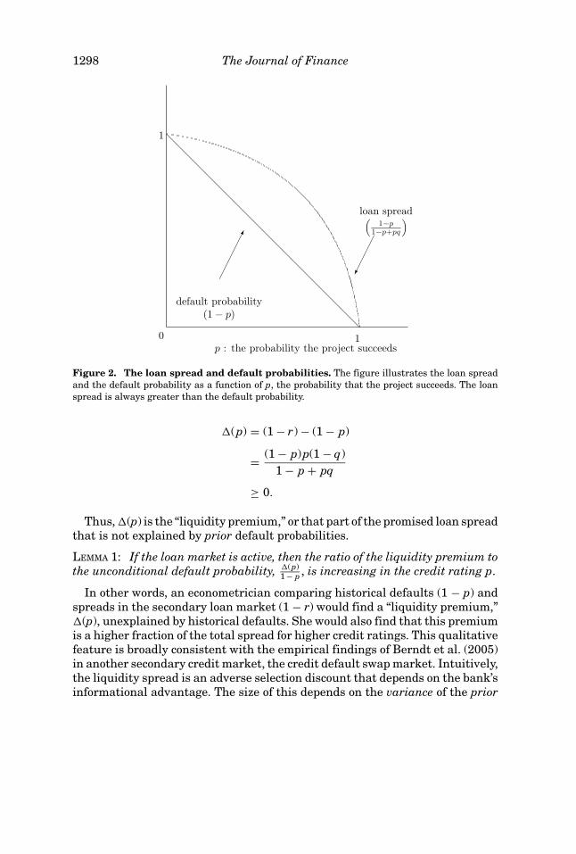
Notice that r < p, the unconditional probability that the project succeeds. Theloan spread in the secondary market incorporates an adverse selection discount.The spread is not given by the unconditional default probability (1 − p); rather,it reflects the probability that the firm defaults conditional upon the fact thatthe bank is willing to sell the risk. This is always weakly higher than theunconditional default probability. Figure 2 depicts the default probability andthe spread in the secondary market.

Let �(p) denote the difference between the promised spread in the secondarymarket and the unconditional default probability:

11 We explore this idea further in Section V.12 We note in passing that a trivial zero trade equilibrium can also be constructed by assigning

the arbitrary off-equilibrium path belief to the bond market that banks with a discount factor shockdo not trade. In such an equilibrium the price is also zero.


1

0 1

loan spread1−p

1−p+pq

default probability(1 − p)

p : the probability the project succeeds

Figure 2. The loan spread and default probabilities. The figure illustrates the loan spreadand the default probability as a function of p, the probability that the project succeeds. The loanspread is always greater than the default probability.

�(p) = (1 − r) − (1 − p)

= (1 − p)p(1 − q)1 − p + pq

≥ 0.

Thus, �(p) is the “liquidity premium,” or that part of the promised loan spreadthat is not explained by prior default probabilities.

LEMMA 1: If the loan market is active, then the ratio of the liquidity premium tothe unconditional default probability, �(p)

1 − p , is increasing in the credit rating p.

In other words, an econometrician comparing historical defaults (1 − p) andspreads in the secondary loan market (1 − r) would find a “liquidity premium,”�(p), unexplained by historical defaults. She would also find that this premiumis a higher fraction of the total spread for higher credit ratings. This qualitativefeature is broadly consistent with the empirical findings of Berndt et al. (2005)in another secondary credit market, the credit default swap market. Intuitively,the liquidity spread is an adverse selection discount that depends on the bank’sinformational advantage. The size of this depends on the variance of the prior


(p(1 − p)). By contrast, the unconditional spread depends only on its mean. Theexpected credit losses decrease faster than their variance as p increases.

B. Characterization of Optimal Contracts

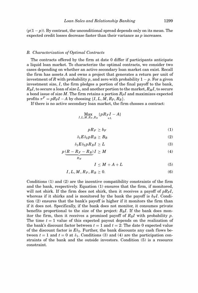
The contracts offered by the firm at date 0 differ if participants anticipatea liquid loan market. To characterize the optimal contracts, we consider twocases depending on whether an active secondary loan market can exist. Recallthe firm has assets A and owns a project that generates a return per unit ofinvestment of R with probability p, and zero with probability 1 − p. For a giveninvestment size, I, the firm pledges a portion of the final payoff to the bank,RBI, to secure a loan of size L, and another portion to the market, RMI, to securea bond issue of size M. The firm retains a portion RFI and maximizes expectedprofits πF = pRFI − A by choosing {I, L, M, RF, RB}.

If there is no active secondary loan market, the firm chooses a contract:

MaxI ,L,M ,RF ,RB

{pRF I − A}s.t.

pRF ≥ bF (1)

δ1 Eδ2 pRB ≥ BB (2)

δ1 Eδ2 pRB I ≥ L (3)

p (R − RF − RB)︸︷︷︸RM

I ≥ M (4)

I ≤ M + A + L (5)

I , L, M , RF , RB ≥ 0. (6)

Conditions (1) and (2) are the incentive compatibility constraints of the firmand the bank, respectively. Equation (1) ensures that the firm, if monitored,will not shirk. If the firm does not shirk, then it receives a payoff of pRFI,whereas if it shirks and is monitored by the bank the payoff is bFI. Condi-tion (2) ensures that the bank’s payoff is higher if it monitors the firm thanif it does not. Specifically, if the bank does not monitor, it consumes privatebenefits proportional to the size of the project: BBI. If the bank does mon-itor the firm, then it receives a promised payoff of RBI with probability p.The time t = 1 value of this expected payout depends on the realization ofthe bank’s discount factor between t = 1 and t = 2: The date 0 expected valueof the discount factor is Eδ2. Further, the bank discounts any cash flows be-tween t = 1 and t = 0 at δ1. Conditions (3) and (4) are the participation con-straints of the bank and the outside investors. Condition (5) is a resourceconstraint.


LEMMA 2: Suppose that there is no active loan market. If 1 + BB1 − δ1 Eδ2

δ1 Eδ2< pR <

1 + BB1 − δ1 Eδ2

δ1 Eδ2+ bF , then the expected profits to the firm, πF(p), the project size,

I(p), the amount borrowed from the bank, L(p), and the amount borrowed fromthe market, M(p), are

π F (p) =pR − 1 − BB

(1 − δ1 Eδ2

δ1 Eδ2

)1 − pR + bF + BB

(1 − δ1 Eδ2

δ1 Eδ2

) A

I (p) = A

1 − pR + bF + BB

(1 − δ1 Eδ2)

δ1(Eδ2)

)M (p) = I(p)(1 − BB) − A

L(p) = BB I (p).

The term BB( 1 − δ1 Eδ2δ1 Eδ2

) in the denominator of I(p) is the unit rent that accruesto the bank. Together with the firm’s unit informational rent bF, this reducesthe fraction of the unit surplus pR − 1 that can be pledged to outside investors,thereby capping total investment size I.

Now, suppose that an active secondary market exists and a bank can sellclaims to t = 2 cash flows at a price r at date 1. The firm then solves:

MaxI ,L,M ,RF ,RB

{pRF I − A}

s.t.

pRF ≥ bF

δ1 pRB ≥ BB + δ1r RB (7)

L ≤ δ1 pRB I (8)

p(R − RF − RB)I ≥ M

I ≤ M + A + L

I , L, M , RF , RB ≥ 0.

The existence of a liquid market changes the bank’s incentive compatibilityand participation constraints (7) and (8) through changes in its discount factor.First, consider the payoff to the bank that monitors the firm: δ1 pRBI. The bankhas been promised RBI if the project succeeds. The bank can sell the claim att = 1 if it finds out the project has failed or if it receives a discount factor shock.Thus, with probability (1 − p + pq) the bank sells its claim at price r = pq

1 − p+pq .


With probability p(1 − q), it will not sell its claim but values it at a discountrate of one. Thus, the expected value of a dollar promised at t = 2 is p, whichthe bank discounts to t = 0 at δ1. If the bank shirks (the right-hand side of (7)),it receives private benefits of BBI. In addition, it knows that the project hasfailed. It can therefore sell its promised payment of RBI at a price of r in theloan market. The t = 0 value of this sale is δ1rRBI.

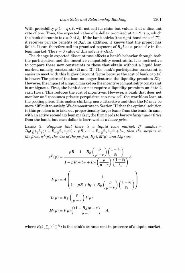
The change in expected discount rate affects a bank’s behavior through boththe participation and the incentive compatibility constraints. It is instructiveto compare these new constraints to those that obtain without a liquid loanmarket, namely, constraints (2) and (3). The bank’s participation constraint iseasier to meet with this higher discount factor because the cost of bank capitalis lower: The price of the loan no longer features the liquidity premium Eδ2.However, the impact of a liquid market on the incentive compatibility constraintis ambiguous. First, the bank does not require a liquidity premium on date 2cash flows. This reduces the cost of incentives. However, a bank that does notmonitor and consumes private perquisites can now sell the worthless loan atthe pooling price. This makes shirking more attractive and thus the IC may bemore difficult to satisfy. We demonstrate in Section III that the optimal solutionto this problem is to take out proportionally larger loans from the bank. In sum,with an active secondary loan market, the firm needs to borrow larger quantitiesfrom the bank, but each dollar is borrowed at a lower price.

LEMMA 3: Suppose that there is a liquid loan market. If max[bF +BB( 1

δ1) p

p − r ; 1 + BBp

p − r1 − δ1

δ1] < pR < 1 + BB

pp − r

1 − δ1δ1

+ bF , then the surplus tothe firm, πF(p), the size of the project, I(p), M(p), and L(p) are

π F (p) =pR − 1 − BB

(p

p − r

) (1 − δ1

δ1

)1 − pR + bF + BB

(p

p − r

) (1 − δ1

δ1

) A

I (p) = A

1

1 − pR + bF + BB

(p

p − r

) (1 − δ1

δ1

)

L(p) = BB

(p

p − r

)I (p)

M (p) = I(p)(

(1 − BB)p − rp − r

)− A,

where BB( pp − r )( 1 − δ1

δ1) is the bank’s ex ante rent in presence of a liquid market.


C. Parameter Restrictions

Lemmas 2 and 3 present solutions to the model under the respective param-eter restrictions:

1 + BB1 − δ1 Eδ2

δ1 Eδ2< pR < 1 + BB

1 − δ1 Eδ2

δ1 Eδ2+ bF ,

if there is no active market, and

max[bF + BB

(1δ1

)p

p − r; 1 + BB

pp − r

1 − δ1

δ1

]

< pR < 1 + BB

(p

p − r

)1 − δ1

δ1+ bF ,

if loan sales are possible. In both cases, the left-hand inequality ensures thatthe project’s NPV is sufficiently high so that the firm can borrow from the bankand the market, and that bank monitoring is feasible. The right-hand inequal-ity bounds the NPV so that the optimal investment size is finite. When weperform comparative statics we assume that these conditions hold; effectively,BB is sufficiently small and bF is sufficiently large. For a fixed R, the conditionsrestrict default probabilities (1 − p) to a small range. Empirically, Hamilton(2001) finds that average 5-year cumulative default rates for investment-gradenames are 0.82% and 18.56% for speculative names. Thus, the interval of de-fault probabilities that we consider is small.

III. Liquidity and Efficiency

By assumption, the bank and bondholders are always held to their partici-pation constraints. Thus, social surplus is maximized when the firm makes thehighest profit. Given the constant returns to scale technology, profits are maxi-mal when the size of the project, I(p), is maximal. Equivalently, social efficiencydemands that a firm borrows as much as possible.

Recall that

I (p) = A

1

1 − pR + bF + BB1 − δ1 Eδ2

δ1 Eδ2

if the loan is illiquid

1

1 − pR + bF + BBp

p − r1 − δ1

δ1

if the loan is liquid.

Thus, a liquid secondary loan market is socially efficient if the bank’s unitrent is smaller when there is active loan trading:

BBp

p − r1 − δ1

δ1< BB

1 − δ1 Eδ2

δ1 Eδ2.


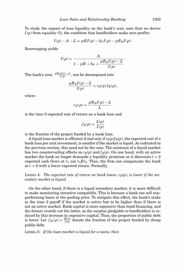
To study the impact of loan liquidity on the bank’s rent, note that we deriveI (p) from equality (5), the condition that bondholders make zero profits:

I (p) − A − L = pR I (p) − bF I (p) − pRB I (p).

Rearranging yields

I (p) = A

1 − pR + bF + pRB I (p) − LI (p)

.

The bank’s rent, pRB I (p) − LI (p) , can be decomposed into

pRB I (p) − LI (p)

= rB(p) f B(p),

where

rB(p) = pRB I (p) − LL

is the time 0 expected rate of return on a bank loan and

f B(p) = L(p)I (p)

is the fraction of the project funded by a bank loan.A liquid loan market is efficient if and only if rB(p)f B(p), the expected cost of a

bank loan per unit investment, is smaller if the market is liquid. As indicated inthe previous section, this need not be the case. The existence of a liquid markethas two countervailing effects on rB(p) and f B(p). On one hand, with an activemarket the bank no longer demands a liquidity premium as it discounts t = 2expected cash flows at δ1 not δ1Eδ2. Thus, the firm can compensate the bankat t = 0 with a lower expected return. Formally,

LEMMA 4: The expected rate of return on bank loans, rB(p), is lower if the sec-ondary market is liquid.

On the other hand, if there is a liquid secondary market, it is more difficultto make monitoring incentive compatible. This is because a bank can sell non-performing loans at the pooling price. To mitigate this effect, the bank’s stakein the time 2 payoff if the market is active has to be higher than if there isnot an active market. Bank capital is more expensive than bond financing, andthe former crowds out the latter, as the surplus pledgable to bondholders is re-duced by this increase in expensive capital. Thus, the proportion of public debtis lower. Let f M (p) = M (p)

I (p) denote the fraction of the project funded by cheappublic debt.

LEMMA 5: If the loan market is liquid for a name, then


(i) The ratio of bank debt over total project size, f B(p), is higher.(ii) The ratio of public debt over total project size, f M(p), is lower.

While the cost of bank capital rB(p) is lower, proportionally more has to besolicited per unit investment to ensure that the bank monitors when the loanis liquid. If the net effect is a reduction in the total surplus paid to the bank,rB(p)f B(p), then investment, I(p), increases. Conversely, if there is an increasein the total surplus accruing to the bank, then I(p) decreases.

Our main result is that this reduction in investment caused by loan salesmay occur for some parameter values. Thus, a liquid secondary market neednot be efficient.

PROPOSITION 1:

(i) A liquid secondary loan market exists if and only if the possible discountfactor shock, δ, is sufficiently small so that δ ≤ pq

1 − p + pq .(ii) A liquid secondary market is socially efficient if and only if the possible

discount factor shock, δ, is sufficiently small so that δ ≤ (1 − q)(δ1 − p)(1−p) − q(δ1 − p) .

The first condition of Proposition 1 requires that for the market to be liq-uid, the pooling price, r = pq

1 − p + pq , must be high enough that banks receivingdiscount factor shocks are willing to sell at this price.

Notice that for a fixed value of δ, an active market is ceteris paribus easierto sustain for higher rated names. Alternatively, for a fixed default probability,liquidity arises when the bank’s private cost of bearing risks until maturity isgreater than the liquidity premium in the loan market. Thus, we should expectto see more loans sold when banks are faced with a higher opportunity costof lending (lower δ). This observation is the basis for our comparative staticsresults in Section IV. The second condition implies that for higher rated names,a secondary market is more likely to be ex ante inefficient.

The condition for efficiency is the threshold below which aggregate invest-ment is larger when the loan is liquid. There are four possibilities in thiseconomy.

Figure 3 illustrates that there can be too much or too little loan trading.Financial institutions may inefficiently lay off low risk projects, leading to loweroverall investment, or may inefficiently retain more risky projects when theiropportunity cost is low.

PROPOSITION 2: If

(1 − q)(δ1 − p)(1 − p) − q(δ1 − p)

< δ ≤ pq1 − p + pq

,

then the secondary loan market is liquid but this is inefficient.

For such parameter values, any commitment device preventing banks fromactively managing their risks would be desirable ex ante. The intuition is asfollows: In our model, loan sales are efficient if they reduce the total cost of loans.


δ

p probability of success

illiquidefficient

liquidefficient

liquidinefficient

illiquidinefficient

Figure 3. Efficiency and Liquidity. Four different combinations of efficiency and liquidity mayexist in an economy. If p, the probability of success, is sufficiently high, then the loan markets areliquid; if the bank’s opportunity cost of capital is sufficiently high (δ sufficiently low), then financialinnovation is efficient.

As we have shown, the expected return on bank loans always decreases withthe advent of a liquid market, as banks no longer demand a liquidity premium.This effect is independent of the credit rating of the underlying name and onlydepends on the bank’s opportunity cost of capital (δ). By contrast, as the creditquality of a firm increases, increasing amounts of bank loans have to be solicitedwith the advent of a liquid market. Loans to firms with high credit quality arevery valuable in the secondary market and thus there is a proportionally largerbenefit to shirking. For large enough p, the quantity effect outweighs the priceeffect and a liquid market is socially inefficient.13

IV. Cross-sectional Implications

In our model, δ corresponds to the bank’s opportunity cost of bearing a loan.Thus, a low δ corresponds to either profitable outside lending opportunitiesand tight financial constraints, or both. In the United States, the Reigle-NealAct removed barriers to interstate banking in 1994. The Basel Capital rulesrequiring banks to maintain capital reserves of 7.25% of loans were adoptedin 1989. The reserve requirement was increased to 8% in 1992. In 1991, theFederal Deposit Insurance Corporate Improvement Act (FDICIA) was passed.Among other provisions, this law mandated “risk-based” deposit insurance pric-ing. Subsequent to the Act’s passage, banks with lower capital ratios paid higher

13 We conjecture that in a dynamic model with reputation effects, higher-rated firms may requireless monitoring.


premia. Thus, in contrast to the late 1980s, the early to middle 1990s werearguably a time when corporate lending became more constrained by legisla-tion while new banking opportunities emerged. We interpret the late 1980s asa period when δ was high and the early to middle 1990s as a period when δ

was low.14 Consistent with this interpretation, in the late 1980s banks shiftedtheir investment portfolios away from corporate loans and into governmentsecurities. Observers interpreted this as a response to the absence of capitalrequirements for government securities in the Basel I rules. Several empiricalstudies (surveyed in Gorton and Winton, (2002)) find some empirical supportfor the hypothesis that this regulatory arbitrage played a role in the “creditcrunch” of the early 1990s.

We posit that the rise of loan liquidity during the 1990s was triggered bythis change in δ, and consider changes in market aggregates that must alsohave occurred over the same period. Formally, consider a population of firmswho differ only in credit ratings. Assume that their success probabilities, p,are distributed on [p

¯, p̄]. We compare the cross-sectional variations of firms’

financial structure for two different values of δ, denoted δ¯

and δ̄, where

0 < δ¯

< δ̄ < 1.

Here, δ¯

is the opportunity cost of lending in the mid 1990s while δ̄ is that ofthe late 1980s. As an active corporate loan market emerged in the 1990s, weassume that the market is illiquid for δ̄, while for δ

¯there is a liquid loan market

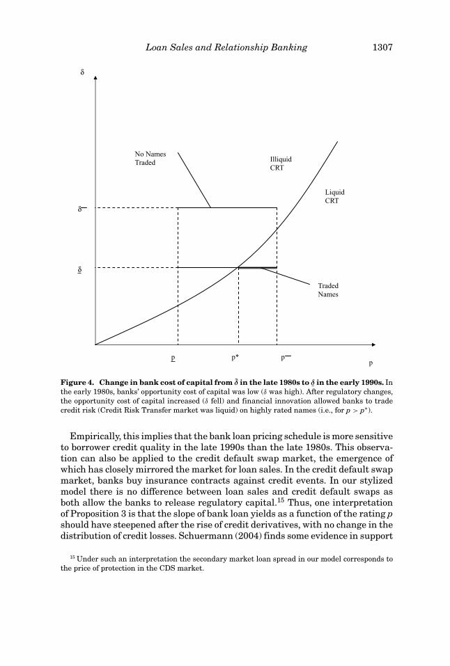
for all p ≥ p∗, where p∗ ∈ [p¯, p̄]. This situation is depicted in Figure 4.

PROPOSITION 3: Suppose δ decreases from δ̄ to δ¯. Consider two firms that differ

by their success probabilities p′′ > p′, where p′′ ∈ [p∗, p̄] and p′ < p∗. Then, theyield spread between bank loans to each firm is larger for δ

¯than δ̄.

If δ = δ̄ the secondary market is illiquid, and the difference in yields betweenfirms with ratings p′ and p′′, denoted �̄, is

�̄ = δ1(p′′ − p′)(qδ̄ + 1 − q).

If δ = δ¯

liquidity arises for ratings above p∗, and the yield spread �¯

becomes

�¯

= δ1(1 − p′)(qδ¯+ 1 − q) − δ1(1 − p′′),

and thus

�̄ − �¯

= −δ1 p′q(δ̄ − δ¯) − δ1 p′′q(1 − δ̄) < 0.

The first term on the right-hand side indicates that the yield has increased forthe nontraded name p′ because of a decrease in δ. The second term correspondsto a smaller yield for the traded name because the liquidity premium vanishes.

14 We focus on a decrease in δ to simplify the analysis. An increase in q yields similar results.


δ

No NamesTraded

TradedNames

LiquidCRT

IlliquidCRT

δ

δ

p p* pp

Figure 4. Change in bank cost of capital from δ̄ in the late 1980s to δ¯

in the early 1990s. Inthe early 1980s, banks’ opportunity cost of capital was low (δ was high). After regulatory changes,the opportunity cost of capital increased (δ fell) and financial innovation allowed banks to tradecredit risk (Credit Risk Transfer market was liquid) on highly rated names (i.e., for p > p∗).

Empirically, this implies that the bank loan pricing schedule is more sensitiveto borrower credit quality in the late 1990s than the late 1980s. This observa-tion can also be applied to the credit default swap market, the emergence ofwhich has closely mirrored the market for loan sales. In the credit default swapmarket, banks buy insurance contracts against credit events. In our stylizedmodel there is no difference between loan sales and credit default swaps asboth allow the banks to release regulatory capital.15 Thus, one interpretationof Proposition 3 is that the slope of bank loan yields as a function of the rating pshould have steepened after the rise of credit derivatives, with no change in thedistribution of credit losses. Schuermann (2004) finds some evidence in support

15 Under such an interpretation the secondary market loan spread in our model corresponds tothe price of protection in the CDS market.


of this phenomenon. He finds that an estimate of the slope for bank loan pric-ing schedules steepened during the 1990s, while its equivalent for bond pricingschedules flattened, if anything.

The proportion of bank financing in the economy should also have becomemore sensitive to credit rating.

PROPOSITION 4: Suppose δ decreases from δ̄ to δ¯. Then, the fraction of investments

that is financed with bank loans becomes more sensitive to the credit rating offirms. Or, for p′ < p∗ < p′′,

f B(p′′, δ̄) − f B(p′, δ̄) < f B(p′′, δ¯) − f B(p′, δ

¯).

In our model, for p > p∗, this fraction shifts from flat for δ̄ to increasing andconvex for δ

¯.

PROPOSITION 5: Suppose δ decreases from δ̄ to δ¯. Then, the fraction of investments

that is financed with bonds decreases for any rating. Or,

f M (p, δ¯) < f M (p, δ̄) ∀p ∈ [p

¯, p̄].

Note that in our model, the difference between loans and bonds is that loansare held by investors with monitoring skills (banks) while bonds are held bypassive investors. In practice, not only banks, but other sophisticated investorswho arguably have monitoring skills (institutional investors, hedge funds) havebecome increasingly active in the loan and private debt markets. Thus, empir-ical tests of Propositions 4 and 5 should compare the fraction of loans and debtthat is privately placed with a small number of sophisticated investors with thefraction of publicly placed bonds.

V. Discussion and Conclusion

A. Trading Credit Derivatives as an Incentive Device

It is instructive to compare our results to those established in Kahn andWinton (1998) and Maug (1998). In a stock market context, they find that along termist large investor may have higher ex ante incentives to monitor afirm when the market for the firm shares has a low informational efficiency.The intuition is that the large shareholder can buy shares in the market thatare undervalued at an interim date because they do not fully reflect the im-pact of her high monitoring efforts on terminal cash flows. In our setting, thiswould correspond to a situation in which the bank could be incentivized bythe prospect of selling credit insurance for the name that she has monitored atdate 1. In our model, a bank that sells protection in the credit derivatives mar-ket reveals that it owns a good loan, and cannot profit from such a trade. This isbecause financially constrained banks would only buy insurance protection inthis model, and thus cannot be used to camouflage a sale of credit protection.


B. Pooling

As in Holmstrom and Tirole (1997), for tractability we abstract from the possi-bility that a bank finances projects that are not perfectly positively correlated.If the bank could finance diversifiable projects, we conjecture that the bankwould find it optimal to sell senior claims backed by the whole pool of projectsin the secondary market. A large financial contracting literature, pioneered byDiamond (1984), demonstrates the benefits from diversification under asym-metric information.

Interestingly, however, the secondary loan market does not seem to applythis rule of maximal diversification in practice. CLOs are often backed by fairlyrestricted pools, and are commonly specialized by country and/or industry. Thispresents a puzzle: The market for individual loans is rapidly growing, whichcontradicts the principle of maximal pooling. This suggests that diversificationcomes at a cost: Potential investors may have different degrees of expertise indifferent asset pools. In this case, selling undiversified claims may increase theparticipation of sophisticated investors in the market for industries or namesfor which they have expertise. Such a trade-off between focus and diversificationis alluded to by practitioners: Lucas et al. (2006) note that “Investors shouldcertainly be wary of deals in which very high diversity scores are achieved bymanagers straying from their fields of expertise.”

C. Signalling

In Section III, we noted in passing that a bank owning a “good” loan that isalso financially distressed cannot credibly signal its type in the secondary mar-ket. This is because the owner of a worthless loan with limited liability wouldalways mimic any contract that does not feature the possibility of negativefuture consumption in case of default on the loan.

Alternatively, assume that the banks owns other long-term assets that canbe costlessly pledged to the buyer of the loan in order to “overcollateralize”the deal, or equivalently to credibly sell the loan with recourse. If the bankpledges a date 2 cash flow of at least 1

δfor each unit of loan sold, then it is not

mimicked by the owner of a bad loan.16 In practice, overcollateralization is likelyto be costly if the bank’s counterparties have a lower valuation of the collateralthan the bank itself. The cost of overcollateralization would then determinewhether a good bank prefers signalling its type to selling the loan at a poolingprice.

D. Perfect Learning

The assumption that the bank perfectly learns the date 2 outcome at date 1is simplifying, but not innocuous. It implies that p measures both the ex ante

16 The (distressed) owner of a bad loan would receive $1 from the loan sale, and lose the collateralat date 2, which has a present cost of $1 at date 1.


riskiness of the project and the ex post informational advantage of the bank.Alternatively, suppose that the bank learns the date 2 outcome with probabilityk ∈ (0, 1). We suggest that our results are robust under the assumption thathigher-rated firms are more transparent, or high p implies low k. To see this,observe that there are now three types of banks trying to trade in the date 1loan market:

1. A bank who knows the loan is nonperforming.2. A distressed bank who knows the loan is performing.3. A distressed bank who does not have an informational advantage.

All such types would trade at the pooling price

r ′ = qpq + k(1 − p)(1 − q)

if r′ > δ. Note that r′ is increasing in p and decreasing in k. Thus, under theassumption that higher-rated firms are more transparent, so that the informa-tional gap between banks and arm’s length lenders is smaller for such firms,then distinguishing between k and p a lower k should reinforce the impact ofa higher p on the price of protection for higher ratings. Similarly, inspectionof the firm’s profit in Lemma 3 shows that it is increasing in the loan spread,1 − r.

E. Basel II Capital Adequacy Rules

In the cross-sectional analysis of Section IV, we studied the situation in whichthe same capital requirement applies to all corporate loans. Specifically, thediscount factor had a constant value δ regardless of the credit rating p. Thisis in line with the Basel I rule imposing the same capital weight of 8% for allcorporate borrowers.

Under Basel II, capital weights are supposed to increase with respect tothe riskiness of loans. In our setting, the introduction of risk-based capitalrequirements corresponds to a situation in which the date 2 discount factorafter a shock is no longer a constant, but is rather an increasing function ofp, δ(p). It is easy to see that such a prudential reform has potentially positiveeffects in our setup, redirecting liquidity in the secondary market to where itis most desirable.

First, for high rated names, for which liquidity is ex ante inefficient, a suffi-cient reduction in capital requirements—namely, a sufficiently large increasein δ—will cause a desirable decrease in liquidity in the secondary market. Con-versely, for lower-rated names that do not trade in the secondary market underBasel I, even though this would be ex ante desirable, a reduction in δ may spurfinancial innovation. In this case, a liquid market is desirable because the costof additional incentives is lower than the benefits from flexibility.

We note that in our model, capital requirements are exogenous costs imposedon banks, and therefore on firms. It seems intuitive that, in the case of high-rated names, a reduction in these costs would be overall welfare improving.


Perhaps more interesting is the result that, for high risk issuers, an increasein this exogenous cost imposed on the economy may actually be welfare im-proving, because this constraint spurs efficient liquidity. The intuition is thatfor sufficiently low-rated names, the negative impact of liquidity on ex anteincentives is limited because the market value of the risk, based on the priorprobability of default, is low.

In sum, we have analyzed the recent rise of a secondary loan market with asimple model of endogenous liquidity. Banks trade actively when they find thatselling a loan is preferable to bearing its risk. Their risks become liquid whenthe benefits from relaxing financial constraints overcome the informationalcost of shedding risks. We posit that because banks’ opportunity cost of car-rying loans has increased, markets have evolved that allow banks to separatebalance sheet management and borrower relationship management. Becauseliquidity implies ex ante inefficiencies, we predict possible excessive trading inhigh-rated paper, and insufficient liquidity in higher-yield tranches. Risk-basedcapital requirements for financial institutions should redeploy liquidity whereit is the most desirable; namely, where the gains in financial flexibility over-come the costs associated with banks’ reduced incentives to develop a long-termrelationship with their borrowers.

Appendix: Proofs

Proof of Lemma 1: Recall that�(p)I − p

= p(1 − q)I − p(1 − q)

,

which obviously increases with respect to p. Q.E.D.

Proof of Lemma 2 and 3: For each of these cases, all the constraints arebinding. The stated results follow. Q.E.D.

Proof of Lemma 4: The promised return per dollar invested is pRB IL . Thus, if

there is a liquid secondary market, this is pRB IL = 1

δ1. If not, then pRB I

L = 1Eδ2δ1

.The result follows from Eδ2 < 1. Q.E.D.

Proof of Lemma 5:

(i) The ratio of bank debt over total project size if there is an active loanmarket is


LLiq

I Liq= pBB

p − r,

and if there is not,

Lno

Ino = BB.

Thus, LLiq

I Liq ≥ Lno

Ino if p ≥ p − r, which always holds.(ii) The ratio of market debt over total project size, if there is no active market

is

M no

Ino = pR − bF − BB1

δ1 Eδ2,

and if there is one,

M Liq

I Liq= pR − bF − BB

pδ1(p − r)

.

Then, M no

Ino ≥ M Liq

I Liq if Eδ2 >p−r

p , which always holds. Q.E.D.

Proof of Proposition 1:

(i) A bank will sell the loan on a failed project at any price r ≥ 0. A bank witha successful project values it at δ2 R, and thus will sell it if rR ≥ δ2 R, or r ≥δ2. If r < δ, then only the banks who know that the project is unsuccessfulwill sell, thus claims are worth zero. If r ≥ δ2, then with probability 1 −p the bank knows the project is a failure, and with probability pq, theproject was a success, but the bank got a shock. Thus, if r ≥ δ2, theexpected value of $1 promised at date 2 is pq + (1−p)0

pq + (1−p) .(ii) Follows immediately from

I = A

1

1 − pR + bF + BB1 − δ1 Eδ2

δ1 Eδ2

if the market is liquid

1

1 − pR + bF + BBp

p − r1 − δ1

δ1

if not. Q.E.D.

Proof of Proposition 2: This is a straightforward consequence of Proposi-tion 1. Q.E.D.


Proof of Proposition 3: If δ = δ̄, there is no market and thus the differencein yields between a firm with p′ and p′′ denoted �̄ is

�̄ = δ1(p′′ − p′)(qδ̄ + 1 − q).

If δ = δ¯

a liquid market arises for ratings above p∗, and the yield spread �¯

is

�¯

= δ1(1 − p′)(qδ¯+ 1 − q) − δ1(1 − p′′),

and thus

�̄ − �¯

= −δ1 p′q(δ̄ − δ¯) − δ1 p′′q(1 − δ̄) < 0. Q.E.D.

Proof of Proposition 4: From Proof of Lemma 5, the ratio of bank debt overtotal project size if there is an active market is

LLiq

I Liq= pBB

p − r,

and if there is not,

Lno

Ino = BB. Q.E.D.

Proof of Proposition 5: From Proof of Lemma 5, the ratio of market debtover total project size if there is no secondary loan market is

M no

Ino = pR − bF − BB1

δ1 Eδ2,

and if there is one,

M Liq

I Liq= pR − bF − BB

pδ1(p − r)

. Q.E.D.

REFERENCESAghion, Philippe, Patrick Bolton, and Jean Tirole, 2004, Exit options in corporate finance: Liquidity

versus incentives, Review of Finance 8, 1–27.Akerlof, George A., 1970, The market for “lemons”: Quality uncertainty and the market mechanism,

The Quarterly Journal of Economics 84, 488–500.Altman, Edward I., Gande Amar, and Anthony S. Saunders, 2004, Informational efficiency of loans

versus bonds: Evidence from secondary market prices, Working paper, NYU (Stern).Berndt, Antje, Douglas Rohan, Duffie Darrell, and David Schranz, 2005, Measuring default risk

premia from default swap rates and EDFs, Working paper, Tepper School of Business, CarnegieMellon University.


Breton, Regis, 2003, Monitoring and the acceptability of bank money, Working paper, LondonSchool of Ecnomics, Financial Markets Group.

DeMarzo, Peter, 2005, The pooling and tranching of securities: A model of informed intermediation,Review of Financial Studies 18, 1–35.

Diamond, Douglas W., 1984, Financial intermediation and delegated monitoring, The Review ofEconomic Studies 51, 393–414.

Drucker, Steven and Manju Puri, 2006, On loan sales, loan contracting, and lending relationships,Working paper, Columbia GSB.

Effenberger, Dirk, 2003, Credit derivatives: Implications for credit markets, Frankfurt Voice,Deutsche Bank Research, July.

Faure-Grimaud, Antoine and Denis Gromb, 2004, Public trading and private incentives, Review ofFinancial Studies 17, 985–1014.

Gorton, Gary B. and George G. Pennacchi, 1995, Banks and loan sales marketing nonmarketableassets, Journal of Monetary Economics 35, 389–411.

Gorton, Gary B. and Andrew Winton, 2002, Financial Intermediation, NBER Working Paper No.W8928.

Greenspan, Alan, 2004, Remarks at the American Bankers Association Convention, New York,New York, October.

Hamilton, David T., 2001, Default and recovery rates of corporate bond issuers: 2000, Moody’sInvestors Service, Global Credit Research.

Holmstrom, Bengt and Jean Tirole, 1997, Financial intermediation, loanable funds, and the realsector, The Quarterly Journal of Economics 112, 663–691.

Kahn, Charles and Andrew Winton, 1998, Ownership structure, speculation, and shareholder in-tervention, The Journal of Finance 53, 99–129.

Kiff, John and Ron Morrow, 2000, Credit derivatives, Bank of Canada Review Autumn, 3–11.Lucas, Douglas J., Laurie S. Goodman, and Frank J. Fabozzi, 2006, Collateralized Debt Obligations

Structures and Analysis (Wiley Finance, Hoboken New Jersey).Lummer, Scott L. and John J. McConnell, 1989, Further evidence on the bank lending process

and the capital-market response to bank loan agreements, Journal of Financial Economics 25,99–122.

Maug, Ernst, 1988, Large shareholders as monitors: Is there a trade-off between liquidity andcontrol? The Journal of Finance 53, 65–98.

Pennacchi, George G., 1988, Loan sales and the cost of bank capital, The Journal of Finance 43,375–396.

Rajan, Raghuram G., 1992, Insiders and outsiders: The choice between informed and arm’s-lengthdebt, The Journal of Finance 47, 1367–1400.

Rule, David, 2001, The credit derivatives market: Its development and possible implications forfinancial stability, Financial Stability Review 10, 117–140.

Saunders, Anthony and Marcia Millon Cornett, 2006, Financial Institutions Management: A RiskManagement Approach (McGraw-Hill).

Schuermann, Til, 2004, Why were banks better off in the 2001 recession? Federal Reserve Bank ofNew York Current Issues in Economics and Finance 10 (1).

Documents

Loan Sales and Relationship Banking