Load-Reuse Analysis: Design and Evaluation

Load-Reuse Analysis: Design and Evaluation

Rastislav Bodik Rajiv Gupta Mary Lou Soffa

Dept. of Computer Science University of Pittsburgh Pittsburgh, PA 15260

{bodik, gupta, sof fa}@cs .pitt . edu

Abstract

Load-reuse analysis finds instructions that repeatedly access the same memory location. This location can be promoted to a register, eliminating redundant loads by reusing the results of prior memory accesses. This paper develops a load-reuse analysis and designs a method for evaluating its precision. In designing the analysis, we aspire for completeness-the goal of exposing all reuse that can be harvested by a subsequent program transformation. For register promotion, a suitable transformation is partial redundancy elimination (PRE). To approach the ideal goal of PRE-completeness, the load-reuse analysis is phrased as a data- flow problem on a program representation that is path-sensitive, as it detects reuse even when it originates in a different instruction along each control flow path. Furthermore, the analysis is comprehensive, as it treats scalar, array and pointer-based loads uniformly. In evaluating the analysis, we compare it with an ideal analysis. By observing the run-time stream of memory references, we collect all PRE-exploitable reuse and treat it as the ideal analysis performance. To compare the (static) load-reuse analysis with the (dynamic) ideal reuse, we use an estimator algorithm that computes, given a dam-flow solution and a program profile, the dynamic amount of reuse detected by the analysis. We developed a family of estimators that differ in how well they bound the profiling error inherent in the edge profile. By bounding the error, the estimators offer a precise and practical method for determining the run-time optimization benefit. Our experiments show that about 55% of loads executed in Spec95 exhibit reuse. Of those, our analysis exposes about 80%.

Keywords: profile-guided optimizations, register promotion, program representations, data-flow analysis.

1 Introduction

Without comparison, caches are the best hardware defense against the von Neumann memory bottleneck. Capitalizing on data locality, caches win by reusing recent memory accesses. How can compilers benefit from these reuse opportunities? In the ideal case, the

Permission to make digital or hard copies of all or part of this work for personal or classroom use is granted without fee provided that copies am not made or distributed for profit or commercial advan- tage and that copies bear this notice and the full citation on the first page. To copy otherwise, to republish, to post on servars or to redistribute to lists, requires prior specific permission and/or e fee. SlGPLAN ‘99 IPLDII 5199 Atlanta, GA, USA (9 1999 ACM l-581 13s083-X/99/0004...$5.00

compiler promotes repeatedly accessed memory locations to registers. Register promotion is the best compiler solution for reducing the memory traffic. By removing redundant loads, it decreases the dynamic operation count and shortens instruction schedules. This paper focuses on compile-time detection of load reuse that is amenable to register promotion. We measure the amount of load reuse in programs, and design and evaluate an analysis for reuse detection.

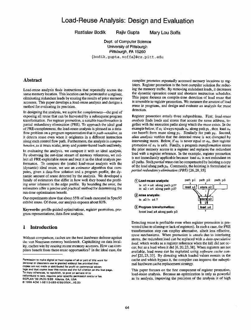
Register promotion entails three subproblems. First, load-reuse nnalysis finds loads and stores that access the same address, together with the execution paths along which the reuse exists. In the example below, if ai always equals a4 along path pi , then load a4 can benefit from reuse along ~1. Similarly for path ~2. Second, alias analysis verifies that the detected reuse is not disrupted by intervening stores. Below, if as is never equal to a4, then register promotion of a4 is safe. Finally, a program transformation stores the prior memory access in a register and replaces the redundant load with a register reference. In the example, register promotion is not immediately applicable because load a4 is not redundant on all paths. Suchpartial reuse can be compensated by hoisting a copy of the load along path pa. Commonly, the hoisting is formulated as partial redundancy elimination (PRE) [26,28,35].

@Load-reuse analysis: is al = a4 along path pl? is a2 = a4 along path ~27

@Alias analysis: is a0 I= a4 7

path pl path p2 path p3

@Program transformation: hoist load a4 along path p3

Detecting reuse is profitable even when register promotion is pre- vented (due to aliasing or lack of registers). In such a case, the PRE transformation step can employ alternative, albeit less effective, reuse mechanisms. When promotion is unsafe due to interfering stores, the redundant load can be replaced with a data-speculative loud, which works as a register reference when the kill did not occur, but as a load when it did [6,20,23,38]. When registers are not available, load reuse can be exploited using software cache control [20,23,33]. By directing which loaded values remain in the cache and which bypass it, the compiler can improve the subopti- mal hardware cache replacement strategy.

This paper focuses on the first component of register promotion, load-reuse analysis. Because an optimization is only as powerful as its analysis, improving the precision of the analysis is of high

64

significance. The second component, alias analysis, has a different aim: while load-reuse analysis detects memory references that must go to the same location, alias analysis finds those that may, thus identifying killing stores. Recent research indicates that, for register promotion, a simple alias analysis may be sufficient [ 18,271. The third component, PRE transformation, was explored in [lo], where we describe how to effect a complete removal of all detected reuse. In this paper we concentrate on increasing the amount of detected reuse.

Design. The design of the load-reuse analysis emphasizes scalability and completeness. Scalability is achieved by developing a sparse, SSA-based program representation, which grows moder- ately with the program size.

The analysis is PRE-complete if it detects all reuse that the PRE transformation can exploit. Aiming for PRE-completeness is not a narrow goal, as PRE covers most scalar transformations based on data-flow analysis. It generalizes common-subexpression elimination, loop-invariant code motion, and constant propagation. Be- yond the power of the PRE class are, however, loop optimizations, such as loop fusion and interchange. These array-oriented transformations can be used as a preprocessing, locality-improving phase, after which PRE can harvest the scalar reuse opportunities [ 131.

To approach PRE-completeness, the load-reuse analysis is path- sensitive and comprehensive. Path-sensitivity has two flavors. First, we can expose reuse even when it exists only on a subset of paths coming to the load (in the example, path ps has no reuse). Second, we find the equivalence of address expressions even when it is path- specific (it is sufficient that al equals a+ along the path p1 and not along all paths). The analysis is comprehensive in that memory references to scalars, arrays or pointer-based data structures are han- dled uniformly, without any high-level program information, such as type information.

Technically, our load-reuse analysis is formulated as a data-flow problem in order to directly guide the PRE transformation [ 10,241. In our analysis, data-flow problems are solved on the Value Name Graph (VNG) [5], a program representation that enhancesdata-flow analysis by exposing equivalence among address expressions. This paper extends the VNG representation in two directions. First, we improve its power by modeling indirect memory references. Sec- ond, because the original VNG [5] did not scale well, we develop a sparse VNG, based on the SSA form [17].

Evaluation. Typically, optimizations are evaluated by reporting the amount of computations removed. Unfortunately, such absolute measure says little about how much potential remains unexploited. Instead, our evaluation measures the level of PRE-completeness: how far is the analysis from an ideal one? Because detecting load reuse is in general undecidable, we can only hope to find an approximation of the ideal reuse amount. For that purpose, we perform a simulation-based limit study: by observing the dynamic stream of memory references, we find all reuse available under a given input and use it as an upper bound of the PRE-exploitable reuse in the program.

While the (static) load-reuse analysis identifies redundant loads and their reuse paths, the (dynamic) limit study yields the run-time number of redundantly executed loads. To compare these disparate quantities, we weight me static reuse using the program profile generated by the simulator. The result is the run-time amount of statically detected redundant loads. This amount can, besides measuring the precision of the analysis, guide the code-duplication trade- offs in code-restructuring optimizations [1,7,8,29,30], as described in [lo]. Unfortunately, any method for computing the run-time

edge profile data-flow solution --.-.-.. T _..__.__

7

-~~~~i

reuse level .... ‘-l-- -..

weighted solution I i .” -” .’ ‘.-I -...’ -.

Section 3

Section 4

Figure 1: The experimental framework, as presented in the paper.

amount of reuse from a profile is impaired by the profile’s inherent inability to precisely reconstruct frequencies of execution paths on which reuse was detected by the analysis. This holds both for the commonly used edge profiles and for the more powerful path profiles, which record frequencies of not just CFG edges but also (some) finite paths [3]. While existing profile-directed optimizations disregard the profiling error [ 10,321, our family of estimator algorithms computes its bounds. The estimators form a hierarchy: the more complex, the tighter the error bounds.

Summary. This paper culminates our efforts in developing a path- sensitive framework for value-flow optimizations [4-lo]. Here, we develop a few missing pieces of the framework (sparse VNG, estimators) and also evaluate its effectiveness (on the load-reuse optimization, using the limit study).

In summary, the contributions of the paper are threefold:

Load-reuse analysis: we generalize the Value Name Graph representation [5] by supporting analysis of indirect memory accesses. We also develop a scalable, sparse version of the representation.

Load-reuse limit study: we develop a simulation-based method for detecting the amount and sources of load reuse in a program and use it to evaluate a static load-reuse analysis. The reuse available in significant benchmarks (Spec95) is reported.

Profile-based estimators: we develop algorithms that use edge profiles to assign a dynamic weight to an analysis- detected reuse. The estimators can be ordered by precision; even modest complexity is enough to use edge profiles and get sufficient precision.

Our entire experimental framework is summarized in Figure 1. Our experiments show that about 55% of loads executed in Spec95 could be removed through reuse. Of those, 80% are detected by our load-reuse analysis.

The rest of the paper is organized as shown in Figure 1. Section 2 describes the simulation-based reuse detection. Section 3 is de- voted to the static load-reuse analysis. Section 4 presents the es-

65

timators and Section 5 evaluates the analysis. Finally, Section 6 concludes by discussing related work.

2 Dynamic Amount of Load Reuse

This section focuses on load reuse visible at run time. We present a simulation-based limit study that has multiple uses: a) measuring the amount of reuse in programs (how large is the optimization potential of register promotion?), b) evaluating the load-reuse analysis by providing a reference point (how close is the analysis to its ideal performance?), and c) tuning the analysis (which are the redundantly executed load instructions?). In this section, we describe the design of our simulation and show that a large fraction (55%) of loads executed in Spec95 exhibits reuse opportunities.

The primary use of the limit study is to evaluate the precision of the load-reuse analysis. The precision is measured as the level of completeness. An analysis is T-complete if it detects all reuse that can be removed from the program with a program transformation T. In this paper, T is thepartial redundancy elimination (PRE) [ 10, 24,281. PRE is a code-motion transformation that can exploit reuse even when it exists only on a subset of execution paths incoming to the redundant load. Therefore, PRE has become the basis of modem register promotion techniques [6,14,26,35].

Unfortunately, detecting load reuse is in general undecidable [3 1] and so no compile-time PRE-complete load-reuse analysis exists. Therefore, we use an empirical, run-time analysis that measures the reuse in the program as the program executes. In order to provide a close approximation of PRE-completeness, this simulation- based limit study should collect all reuse that PRE can remove, but no reuse that is beyond PRE’s power. The simulation should thus mimic the character of the PRE transformation.

PRE removes redundancy by (conceptually) hoisting the partially redundant load against all control flow paths until it reaches a memory operation that generates the reuse. At this point, the contents of the promoted memory location is stored in a register that carries it to the original load. The reused valued can be carried for a small number of loop iterations, using multiple registers [5,14,37]. In summary, the PRE operational restriction is that the redundant load can reuse a result of some other static instruction (or itself), where the result must be a small number of dynamic instances old.

The simulation algorithm reflects this PRE property. The run-time reuse is detected by remembering for each static memory instruction its access history: the dynamic stream of its recent addresses. A dynamic instance of a load is then redundant if a prior load or store accessed the same location without an intervening store. If an intervening store did occur, the load is still redundant; the intervening store becomes the reuse source.

As mentioned above in passing, the design of the simulation technique has two contradictory goals. On the one hand, the limit study should yield an upper bound: each reuse that can be removed with PRE must be detected. On the other hand, the bound should be tight: if a reuse for a given static load is intermittent (e.g., because it is sporadic or input dependent), it should be filtered out as noise. In the example below, the reuse between recurrent array accesses (i.e., between the store of A[i + 21 and the load of A[i]) is PRE- exploitable by allocating two registers that will carry the value for two iterations [6,12,14]:

for (i=O; i<N-2; i++) { A[i+2] = A[i]; )

On the other hand, the reuse below is noise. While some consec-

utive loads from the hash table may access the same location, the reuse is not guaranteed to occur each time the program takes the path across the loop backedge. Therefore, PRE cannot exploit this reuse.

while (c=readO) { _. = hashtab[hash(c)]; }

To verify the PRE requirement that a path carries its reuse each time it is followed, the simulator would have to do extensive bookkeep- ing of followed paths. Consequently, we favor a noisier (less tight) upper bound on reuse over an expensive simulation. To reduce the noise, we limit the number of memory cells remembered in the access history of each static load and store. A small number h (1 to 4) of recent accesses is sufficient to capture most loop carried reuses, like the first example above [ 151.

As pointed out in Section 1, PRE is not capable of exploiting loop- level reuse, like the one between loads a and b below. Hoisting b does not work. Instead, the loops must be merged using loop fusion [ 131, after which PRE can harvest the reuse.

for (i=O; i<N; i++) { a: . . = A[i]; } for (i=O; i<N; i++) { b: . . = A[i]; }

The simulation algorithm will (correctly) not identify the load b to be redundant (unless N 5 h) because the access history remem- bers only last h accesses made by load a. Hence, the simulation is consistent with the power of PRE.

Reuse Level. Figure 2 plots the amount of simulation-observed load reuse. For each benchmark, the experiment was carried out at three points in the compilation: for the original program, after optimizations, and after register allocation. The compiler used was the latest public release of Impact [ 161; the optimizations included the local, global, and loop invariant redundant load elimination, as well as superblock optimizations [22]. Note that while in the floating- point benchmarks (the four on the right) the removal of many loads was accompanied by the decrease of observable reuse, in the integer benchmarks the optimizer left many redundant loads unoptimized, which suggests that programs with complex control flow require more powerful, path-sensitive optimizations and/or better alias information. Also note the increase in observed reuse after register allocation, which is due to spill-code loads (the target processor was PA-7100).

We show the amount of reuse for the history depth 1 and 4. In- creasing the history depth raises the observable reuse much more in integer programs than in the scientific ones, where more recurrent accesses would be expected. A manual examination of simulation results strongly suggests that the additional reuse collected at the deeper access history is mainly noise, similar to the intermittent reuse in the hash-table example above. Also shown in the graph is the fraction of reuse in which both the generator and the redundant load belong to the same procedure. These reuse patterns are not strictly intraprocedural, as the procedure might have returned and been called during the reuse. However, these “intraprocedural” reuse levels serve as a reference point for our intraprocedural load-reuse analysis (Section 5).

Input Variance. Profile-directed optimization and simulation- directed optimization design are valuable only if the program input exercises input-independent, pervasive program characteristics. How much does reuse vary across different inputs? We modi- fied the inputs on several benchmarks and compared the observed reuse. The results are shown in Table 1. The input-based variation of the reuse level is within 18%, which may suggest that reuse is

66

Jss- source program; after optimization; after register allocation.

0 all reuse (history=4) all reuse (histoty=l)

+ intraproc reuse 1 (histoly=4)

Figure 2: Simulation-observed load reuse. (Inlining: up to 50% code growth; Spec95 input set: train.)

benchmark input reuse % reuse from % l+S before opti train I test h=4 loads stores lo6

1 8 sueens 1 87.4 76.2 43.6 1 324

Table 1: Sensitivity of load reuse level to program input. The column l+s gives the number of executed loads and stores.

largely input independent. The greatest difference is in m88ksim, in which each input directs the execution into different procedures. For the same reason, this benchmark has less reuse generated by stores in the test input (fractions add up to more than lOOY$ as a reuse instance may be generated by multiple instructions, a load and a store). We have manually examined compress and discovered that the lower reuse in the larger input is due to fewer noisy loads. Input variance may therefore be useful as a noise reduction mechanism; by taking intersection of reuse detected on different inputs, we may determine regular, statically detectable reuse.

Simulation Memory Requirements. While the simulation limit study is considerably more expensive than control flow profiling, it is used once (to design and tune the analysis) unlike the cheaper profiling which is repeated (to optimize each program). Still, the simulation speed was acceptable, at about 9.4 seconds per 1 million loads and stores executed (on PA-8000). The memory required varied greatly. The largest data structures were needed by swim (103MB + 32MB hash table) and the smallest by compress (4MB + the same hash table).

3 Load-Reuse Analysis

While the previous section described the approximate dynamic load-reuse analysis, this section presents the conservative static analysis.

Detecting load reuse reduces to finding path-sensitive must-alias information: we want to know which address expressions are always equivalent and along which control flow paths.’ Our analysis is formulated as a data-flow analysis, for two reasons. First, when detected reuse is expressed as a data-flow solution, it can directly guide the subsequent PRE transformation, which is driven by the data-flow problems of availability and anticipability [ 10,241. While the former problem exposes the reuse (by finding a prior load or store), the later verifies whether the PRE transformation is not harmful to the program (by determining whether the reuse can be consumed by a future load). The second reason is that data-flow analysis can leverage existing program representations [5,6,11,19,37] designed to expose reuse not accessible to the traditional data-flow analysis [24,28].

The analysis in this paper is based on the Value Name Graph, a value-centric representation that enhances traditional data-flow analysis by appropriately naming the value that flows between equivalent computations [5]. A valuejows between two (address) expressions if they compute the same value (address). In traditional data-flow analysis, each value is identified with its lexical name, e.g., its abstract syntax tree. When two names match, the addresses (may) compute identical values. But what name should be used when the value Bows between equivalent addresses that have dif-

‘Recall that the use of may-alias information to disambiguate intervening stores is conceptually independent from detecting load reuse, as described in Section I. This section also shows how may-aliasing is accounted for in our load-reuse analysis.

67

ferent names? The VNG overcomes the naming problem by synthe- sizing names that fully trace the flow of the analyzed value and by performing data-flow analysis on this synthesized name space. The synthesized names are created using symbolic substitutions along each control flow path; as a result, the VNG exposes equivalences among address expressions that become visible only after symbolic algebraic manipulations.

This paper addresses two deficiencies of the original VNG [5]. The first is the lack of expressiveness specific to detecting load reuse. Because the VNG only models value flow through arithmetic computations, it cannot trace flow of addresses through the memory, and hence cannot handle indirect addressing. The second deficiency is the high memory demands of the original VNG, a con- sequence of its rigorous reflection of algebraic characteristics of the value flow. In this paper, the VNG is made more effective by incorporating indirect addressing into the symbolic interpretation, and more eficient by developing a sparse VNG representation that is smaller and scalable.

Constructing the VNG. The VNG combines advantages of three orthogonal analysis approaches. Each of them overcomes different obstacles in equivalence detection: global value numbering finds equivalent expressions that have different names due to assignments to temporaries [34]; symbolic interpretation finds equivalences requiring algebraic simplification, such as recurrent array accesses [6,12]; data-flow analysis connects expressions that may be equivalent only along some control flow paths [24,28]. First, we sketch the construction of the original VNG enhanced to accommodate indirect addressing. The following subsection describes how to build the sparse VNG.

The construction has three steps, each corresponding to one of the underlying approaches. First, the symbolic interpretation creates names necessary to trace the value flow. Second, value numbering determines which names are synonymous references to the same value. The result of the first two steps is the VNG representation, on which the third step computes value-related data-flow problems, using any traditional data-flow analyzer.

Step 1: Create the symbolic names. The goal is to create sufficient names so that a value can be identified even when it flows outside the scope of the lexical name under which it was originally computed. Where the original name is not valid, we use an equivalent symbolic name. The symbolic names are created on demand by propagating backwards the address operand of each load. The propagation effectively creates a “symbolic” slice of the address operand, by substituting into the propagated address expression each relevant assignment and performing some algebraic simplification. While the original address operand represents the lexical name of the address value, the slice expression is the symbolic name. Below, we analyze the address of the load; its lexical name is y + 4. After this name is propagated through the preceding assignment, the name of the address changes to 2 x x + 12, which is a symbolic name. Note that the symbolic substitution was followed by algebraic simplification.

y:=2xx+8 tname=2xx+12

z:= load(y+4) tname=y+4

Due to loops, such a back-substitution process may not terminate. Therefore, we perform the substitution only for w iterations of each loop, where w is a small constant (1 to 4), analogical to the access history h used in the simulation in Section 2.

To accommodate indirect addressing, we enrich the symbolic language of value names with a pointer dereferencing operator * and

back-substitution rules for loads and stores. Loads increase the indirection level: when a name t + 1 is propagated backwards across t := load L, it will change to *L + 1. Stores may reduce the indirection: across store L, t, the name *L + 1 will change to t + 1.

To obtain the performance reported in Section 5, it was sufficient to represent addresses with a symbolic name E = co + c1 v1 + . . . + cnun + *(El), where c; are literals, Vi are program variables, and E’ = E 1 c. The term E’ adds addressing indirection. In the actual implementation, one may want to set a maximum number of indirection levels, to limit the number of symbolic names created during back-substitution. In our experiments, we used level 0 (no * operator in the address name) and level 1 (one * operator in the address).

Figure 3(b) shows the VNG for the program in Figure 3(a). We illustrate the back-propagationusingpa, the address operand of the load in node 9. When propagatingpd across the assignment p4 := ps + 1 in node 7, the right-hand side p3 + 1 is substituted into the current name ~4. We obtain p3 + 1, which becomes another name for the analyzed address of the load (9). After crossingps := load L, in node 6, *L, is substituted for ps and *L, + 1 becomes yet another name for the address (LP is the address of the global variable p). The name will be further changed at nodes 4,3, and 1. (Note that the Figure 3(b) is showing the VNG construction only along the then path) The address operands of remaining memory operations will also undergo this back-propagation. The process of name creation is demand-driven, as only the necessary names are created.

When back-substitution is completed, the graph contains value threads that connect the different names of the analyzed value. Along the control flow path associated with a value thread, the threaded names refer to the same value. Therefore, all memory operations on a thread access the same memory location.

Step 2: Find synonymous names. The value threads are used by data-flow analysis to compute availability of prior memory accesses. For example, reuse exists between nodes 4 and 6, as they lie on the same thread. Unfortunately, threads alone cannot find reuse between the equivalent nodes 5 and 9, because they are not on the same thread. However, their address expressions (tl andp4) are both symbolically reduced by the back-propagation step to the same name ~1, at the entry of node 2. This proves that both of these memory references must access the same memory location; the names from the two parallel threads are synonymous at each node, as expressed by the dashed edges.

We call the second step symbolic value numbering, as it extends the standard global value numbering [34] with the symbolic ma- nipulation. It finds the synonymous names by “collapsing” the threads in a forward pass. Collapsing is performed by inserting store *L, + 1 onto the thread connected with the dashed edge. The new store writes to the same location as its synonymous counter- part ( store tl) but is placed on the parallel thread, which enables detecting the reuse between node 5 and 9. The insertion of the store completes the VNG construction.

Step 3: Solve data-jlow problems. Once the VNG is constructed, any conventional data-flow analysis can propagate facts along the threads augmented by the second step and answer the two ques- tions posed by the PRE transformation: which memory accesses are equivalent, and along which control flow paths? In our example, the reuse between store (5) and load (9) will be revealed in the form of a memory access being available at node 9.

The Sparse VNG. Experiments with the original VNG (shown in Figure 3(b)) revealed three sources of inefficiencies preventing

68

load p

t :=p

P- -

store p

load p

++p

store p

p1 = load L,

4 1

h = Pl 2 i

PZ = Pl - 1

i 3

store L, , pz 4

i store tl,v 5

p3 = load L,

i 6

P4 = PS + 1 7 i

store L,, p4 8 ,

+ I I

w := *p w = load p4 I 9

P: global

if ( ) *p-- z v;

w = *++p;

(a) the source program. (h) the original VNG.

__c

1 bll := [*&,I 9

load [LPI

[ [hl := [pll h

I 1 [P2 + 11 := [pll

4

i_ * ([*Lp + 112 := qq[*L, 4- 1109 [*‘h + Ql

[*Lp + 111 := [pz + l] store [LPI

I

4 store [tl]

1 [ps + 11 := [*Lp + iI2 load Lb1 1

1 b41 := [p3 + 11

load Cl 1

I 1

I 2

I 1

4 I 3

store Cl i

4

store C2 5 4

b := d(Co,C2)

4 load Cl

1

6

r 1

I 7

store 9 J

8

load Ca 9

Congruence classes: co: U*L* + 110) 6: WPlI c2: ~[*bJ7b11,P11,b2 + ll,[*Lp+ 111)

G: {I*-& + llz,I.Ps + 11, fP41)

(c) the SSA fom of VNG.

Figure 3: The Value Name Graph. The original form, and the construction of the Sparse VNG.

practical deployment. First, the synonym relationships are maintained at each node, consuming much memory. Second, many symbolic names do not belong to any value thread on many nodes, wasting slots in data-flow bit-vectors. Such a construction runs out of 1GB virtual memory on some procedures that grew during inlining. Last, threads contain many switches between symbolic names, which reduces bit-vector parallelism, slowing down the analysis. We present here a sparse VNG representation. It reduces memory and time requirements, while maintaining the same power as the original formulation. The memory savings are more than 30-fold on some large procedures.

To obtain the sparse form, we skip the expensive Step 2 above and transform the VNG created in Step 1 into an SSA program with the following (local) transformation: first, for each symbolic name e we create a scalar variable, denoted [e]. Second, at CFG nodes where a name ei is back-substituted into e2, we insert the assignment [el] := [es]. Figure 3(c) contains the result of such transformation. The memory references are correspondingly rewritten to refer to these new variables.

In this intermediate form, each [e] variable will receive an SSA subscript after which the synonyms can be maintained globally using the global value numbering (GVN) [34], rather than on each node, which fixes our first deficiency. In our example, only [*Lp + l] needs an SSA subscript and a &node. After GVN places the [e] variables into congruent classes, the memory references can refer to the class names, which serve as names for all the synonymous names in a class. After converting to class names, the [ei] := [ez] assignments can be removed. The result is the sparse VNG shown

(d) the Sparse VNG.

in Figure 3(d). The rewriting process that led to the sparse VNG removed from value threads many switches (some will remain at 4- nodes, such as that between C’s and C’s) and made the name space denser (four class names versus eight symbolic names), thus fixing the remaining two deficiencies. Additionally, having the SSA properties, the sparse VNG can be implanted into existing SSA-based PRE implementations, improving their precision [26].

Killing stores. The VNG analysis detects reuse aggressively. Because the value threads extend uninterrupted across potentially killing stores, the VNG detects instructions that always read from the same location but it does not reflect that a store may change the contents of this location between these two reads. This exclusive focus on must-aliasing is an intentional design decision; by sep- arating the killing effects, the VNG can detect a weaker form of reuse, one that may occasionally be interrupted, and exploit it with data-speculative loads, as mentioned in Section 1.

The killing information expressed as may-alias information can be accommodated in a natural way when data-flow analysis is computed on the sparse VNG. Using our running example, assume that p4 may equal L,. Because [p4] belongs to congruent class CS and [LPI belongs to Ci, each store to Ci must kill reuse in class CS and vice versa. Therefore, in Figure 3(d), the store in node 8 would kill the reuse for the load in node 9. Depending on the optimizer, this kill may entirely destruct the reuse, preventing register promotion, or may mark only the reuse as unsafe, enabling its exploitation using a data-speculative load [20,23,33].

69

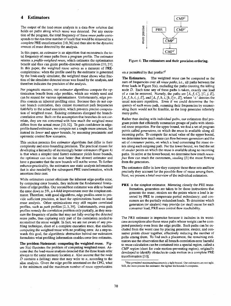
4 Estimators

The output of the load-reuse analysis is a data-flow solution that holds on paths along which reuse was detected. For any execution of the program, the total frequency of these reuse paths cone- sponds to the run-time number of loads that would be removed by a complete PRE transformation [10,36] and thus also to the dynamic amount of reuse detected by the analysis.

In this paper, an estimator is an algorithm that reconstructs the total frequency of reuse paths from a program profile. The estimator returns a projile-weighted reuse, which estimates the optimization benefit and thus can guide profile-directed optimizations [lo, 211. In this paper, the weighted reuse serves as a measure of PRE- completeness: when the profile used by the estimator is generated by the limit-study simulator, the weighted reuse shows what fraction of the simulator-detected reuse was found by the analysis, and therefore indicates the precision of the analysis.

For pragmatic reasons, our estimator algorithms compute the optimization benefit from edge profiles, which are widely used and can be reused for various optimizations. Unfortunately, edge profiles contain an inherent profiling error. Because they do not capture branch correlation, they cannot reconstruct path frequencies faithfully to the actual execution, which prevents precise computation of weighted reuse. Existing estimators disregard the branch- correlation error. Built on the assumption that branches do not cor- relate, they are not concerned with how much the weighted reuse differs from the actual reuse [ lo,32 1. To gain confidence in edge- profile-based estimates, we compute not a single reuse amount, but instead its lower and upper bounds, by assuming pessimistic and optimistic control flow scenarios.

This section presents five estimator algorithms that differ in their complexity and error-bounding precision. The practical reason for developing a hierarchy of increasingly better estimators (Figure 4) is that when a simpler (and faster) estimator yields loose bounds, the optimizer can run the next better (but slower) estimator and have a guarantee that the new bounds will not be worse. To further enhance practicality, the estimators use static analysis information that is also needed by the subsequent PRE transformation, which amortizes their cost.

While estimators cannot eliminate the inherent edge-profile error, by computing error bounds, they indicate the fundamental limitations of edge profiles. Our second best estimator was able to bound the error down to 5%, a 4-fold improvement over the simplest estimator. Therefore, with good algorithms, edge profiles seem to provide sufficient precision, at least for optimizations based on load reuse analysis. Other optimizations may still require correlated profiles, such as path profiles [2,3,39]. Unfortunately, even path profiles remedy the correlation problem only partially, as they measure the frequency of paths that may not fully overlap the detected reuse paths, thus capturing only part of the correlation needed to reconstruct the reuse weight. In fact, we are not aware of any profiling technique, short of a complete execution trace, that enables computing the weighted reuse with no profiling error. As a step to- wards this goal, the algorithmic abstraction behind our estimators formulates what profiling information enables error-free estimates.

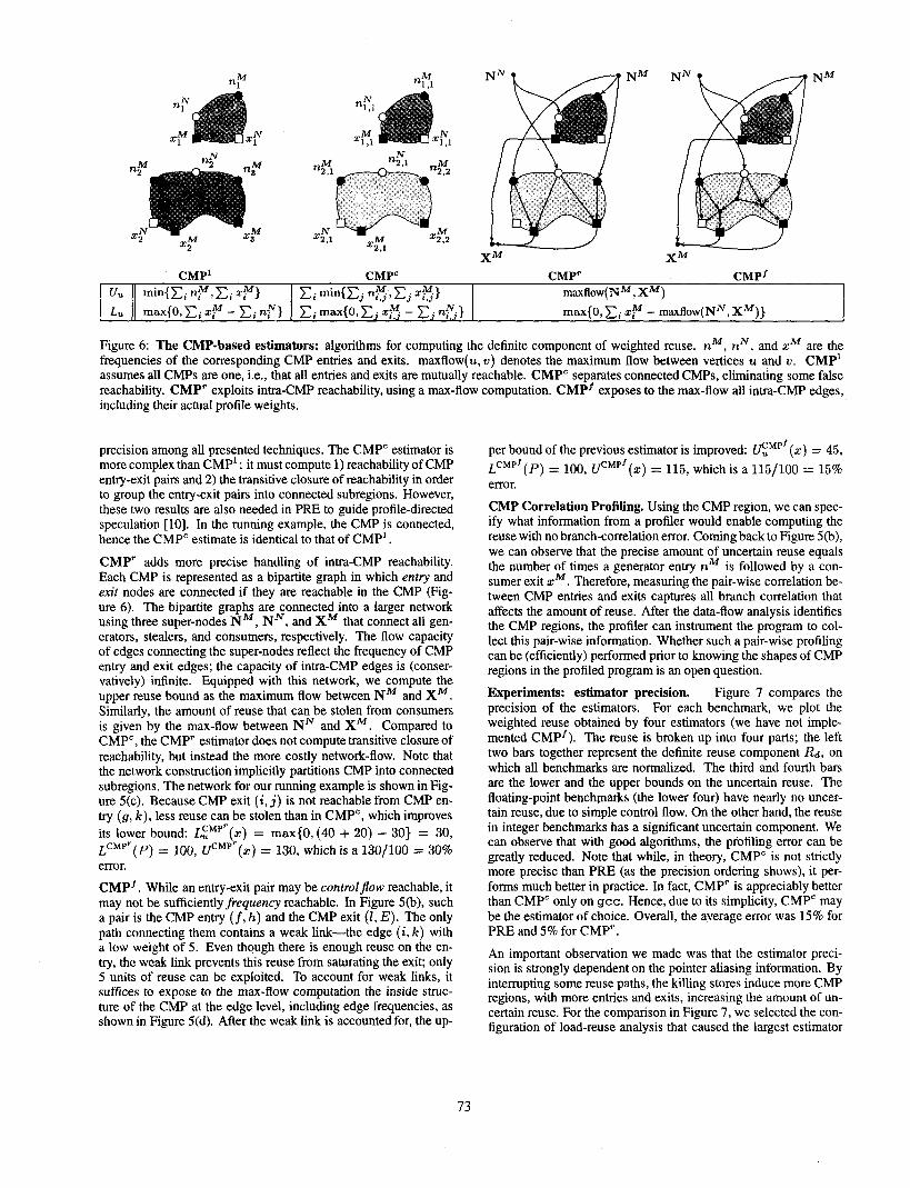
The problem Statement: computing the weighted reuse. Fig- ure 5(a) illustrates the problem of computing weighted reuse. As- sume that the load-reuse analysis detected that the three loads refer always to the same memory location P. Also assume that the node D contains a (killing) store that may write to x, according to the alias analysis. Given the edge profile annotated on the CFG, what is the minimum and the maximum number of reuse opportunities

.g j piq p&q ai ,/’ 2 j ... ,,: 0 : E ! ~iqzl CMP’

i

I CMP’

Figure 4: The estimators and their precision ordering.

on z permitted by that profile?’

The Estimators. The weighted reuse can be computed as the sum of frequencies over all reuse paths, i.e., all paths between the three loads in Figure S(a), excluding the paths crossing the killing node D. Each time any of these paths is taken, exactly one load of z can be removed. Namely, the paths are [A, f, c], [C, j, E], [A, f, h, i, j, E], and [A, f, h, i, [lc, 1]+, E], where ‘+’ denotes the usual non-zero repetition. Even if we could determine the frequency of each reuse path, summing their frequencies by enumer- ating them would not be feasible, as the loop generates infinitely many paths.

Rather than dealing with individual paths, our estimators find program points that efficiently summarize groups of paths with identical reuse properties. For the upper bound, we find a set of program points called generators, on which the reuse is available along all incoming paths. To compute the actual value of the upper bound, we determine how much reuse can flow between generators and the set of consumer points, on which a load consuming the reuse exists along each outgoing path. For the lower bound, we find the set of stealer points on which the reuse is available along no incoming paths. To arrive at the lower bound, we determine how much reuse- free flow can reach the consumers, stealing [3] the reuse flowing from the generators.

The estimators differ in how they compute these three sets and how precisely they account for the possible flow of reuse among them. Next, we present a brief overview of the individual estimators.

PRE is the simplest estimator. Mirroring closely the PRE transformation, generators are taken to be those instructions that generate the reuse; stealers are the points where a load is in- serted by PRE to compensate partial redundancy; and consumers are the partially redundant loads. To determine which generators (or stealers) may provide (or steal) reuse for each consumer load, PRE uses control flow reachability.

The PRE estimator is imprecise because it includes in its worst- case assumptions also those reuse paths whose weight can be computed precisely even from the edge profile. Such paths can be excluded from the worst case by placing generator, stealer, and consumer points closer together, effectively reducing the number of paths among them. To find such a placement, the remaining estimators use the observation that all branch-correlation error harmful to reuse calculation can be contained into a special region, called a Ch4P region (short for code-motion-preventing region), originally developed to identify obstacles to code motion in a complete PRE transformation [ 101.

*The peninerl minimum/maximumis a tight bound. Our estimators are not tight. Still, the more precise the estimator, the tighter the bounds it computes.

70

(a) The source program annotated with an edge profile.

CMP region entrim E 0 Must-Avail

“4 / nN 0 No-Avail

(b) The CMP region for the reuse on memory location x.

actual flow capacity (the weak link IS exposed) - - innntte flow capacity

(c) CMP’estimator, based on control-flow reachability.

(d) CMPfestimator, based on frequency reachability.

Figure 5: An example of computing the weight of load reuse from the edge profile.

The CMP is the smallest multi-entry, multi-exit region in which the entries can be divided between generators and stealers, and the exits between consumers and (strict) non-consumers. Being the smallest such region, it finds the desired closest placement, considering in concert all reuse paths, not only those leading to a single load. The CMP contains all the error because, on each node in the CMP, the reuse is generated only along some incoming paths and can be consumed by a load only along some outgoing paths. Consequently, without the knowledge of branch correlation in the CMP, it is not possible to determine how much incoming reuse actually flowed to consumers in the profiled program execution. On the other hand, outside the CMP region, the reuse can be computed without an error. The CMP estimators thus focus on reducing the error contained in the CMP region, as follows:

The Algorithms. Next, we present the estimators in more detail. Each estimator e returns upper and lower bounds on the total reuse in the program P, which are denoted V(P) and L”(P), respectively. Also, f(d) denotes the execution frequency for d, where d is a CFG node or edge. Finally, L(P) denotes the set of loads in program P.

CMP’ estimator conservatively assumes that there is a single CMP (hence the 1 in the name), in which all entries and exits are mutually reachable. This false reachability may connect consumers to spurious generators and stealers, producing loose bounds.

PRE. The reuse bounds are calculated separately for each consumer point, i.e., for each static load. The sum of bounds over all loads then bounds the total program reuse. For each load 1, we find the generator set G(1) of loads and stores that generate the reuse for 1. The set G(Z) contains those loads and stores that are backwards reachable from 1 along some (kill-free) reuse path. Also through reachability, we find the stealer set of CFG edges S(1) onto which PRE would insert a load to make 1 fully redundant. The reachability is computed on the sparse VNG, shown in Figure 3(d), where store Cz is backwards reachable from load Ca, across the +-node.

CMP” attacks false reachability by partitioning the CMP region into connected CMP subregions, using control-flow reachability between CMP entries and exits. The individual connected CMPs are treated with the CMP’estimator.

To compute the upper bound on the reuse detected for load 1, we assume the most optimistic control flow scenario that all reuse generated in G(Z) flows to 1. In other words, the frequency of reuse paths between G(2) and 1 equals the lower of Z’s and G(l)‘s frequencies. The lower bound assumes the worst case: all flow from stealers reaches 1, maximizing the frequency of reuse-free paths that reach 1; the remaining paths must be reuse paths originating at the generators. Hence we get: (the max operator makes the lower bound non-negative)

CMP’ exploits entry-exit reachability further. Compared to CMPC, it removes false reachability even within each connected CMP, by computing reuse as a network flow problem. the PRE estimator:

CMP’ exposes to the network Bow computation all the CFG edges in the CMP, not just the summary entry-exit reachability information, thus exploiting a refined notion of reachability that accounts for how much reuse can flow between CMP entries and exits, and not just whether they are reachable.

UPRE(P) = C mW(l), C f(s)1 la(p) &JEW

LPRE(P) = C maxi&f(l) - C f(s)1 &L(P) .eS(9

CMP Correlation Profiling estimator is not based on edge pro- Let us apply the PRE estimator on the program in Figure 5(a). files. Instead, it assumes profile information that correlates The bounds for loads A and C are trivial. as A is not redun- CMP entries and exits sufficiently to avoid the profiling error. dant and C is fully redundant: LPRE(A) = UPRE(A) = 0 and

71

LPRE(C) = UPRE(C) = 35. The profiling error affects only the partially redundant load E. Its generators and stealers are G(E) = (4 Cl and S(E) = ((9, h), (a k), (0, E)), yielding bounds LPRE(E) = 45 and UPRE(E) = 135. The total reuse for the program is LPRE(p) = 80 and UPRE(p) = 170, which is a 170/80 = 112.5% error.

The large PRE’s error is not all due to the inherent deficiencies of the edge profile. The cause of the error is “overbooking” of a generator by multiple consumers. In Figure 5(a), load A is a generator common to consumer loads C and E, which together con- sume more reuse than A can generate (C counts 35 and E counts 100). Technically, the cause of overbooking is that PRE charges the entire frequency contribution of a generator to multiple reuse paths that originate in the generator. Instead, the generator frequency should be divided among these paths. This can be done by moving the A generator into the edges (f, C) and (f, h), which become the new generators, effectively dividing the contribution of A among loads C and E. The CMP region is an abstraction that divides the contribution of generators, stealers, and consumers. The CMP region for the running example is shown in Figure 5(b); it effectively excludes the reuse path [A, f, c] from the worst-case considerations.

First, we present the definition of the CMP region. Formally, the CMP is a subgraph of the Sparse VNG. To simplify the presenta- tion, we establish the restriction that the sparse VNG contains no &nodes. Under this restriction of generality, each memory location has exactly one name. Without having to switch names, we can reason about estimators using the CFG, rather than the more general VNG.3While the estimator extensions to handle an arbitrary VNG are small, their explanation is beyond the scope of this paper and can be found in [4].

Given the restriction, the CMP region is identified by solving the problems of anticipability and availability, which are defined as follows [ 101.

Definition 1 Let p be any path from the CFG start node to a node n. The contents of memory with address z is available at n along p iff 2 is loaded or stored on p without a subsequent killing store. Let P be any path from n to the CFG end node. The load of address x is anticipared at n along r iff z is loaded on r before any killing store or a store to x. The availability of z at the entry of n w.tt. the incoming paths is defined as:

1

Must all AVAIL&a, x] = A/o if x is available along no paths.

May some

Anticipability (ANTIC) is defined analogously.

Definition 2 The CMP region for address x, denoted CMP[X], is a set of nodes n where AVAILi,[n, Z] = May and ANTICin[n, x] = May.

Figure 5(b) shows the CMP region for the address x. Each CMP region has a set of entry edges and exit ed es. Each entry is either Must- or No-available; we denote them n If and nN, respectively. The nM entries act as generators and the nN entries act as stealers. Similarly, exits are either Must- or No-anticipated, denoted xM and xN, res;eecti,vely. The x M act as consumer points. The non- consumer x exits do not participate in the estimator algorithms.

‘Note that a sparse VNG (Figure 3(d)) without name switches could still contain name switches in its intermediate (dense) form (Figure 3(b)).

The CMP is the smallest region in which reuse is uncertain; generators cannot be moved closer to consumers, because they would en- ter the CMP regions, where reuse is not available along all incoming paths and thus they would no longer act as generators. Identi- cal arguments prevent moving stealers and consumer points. The CMP thus maximizes the number of paths that can be excluded from the worst-case assumptions about branch correlations; outside the region, the reuse can be computed without any error, even from an edge profile. It can be shown that all reuse bypassing the CMP region can be measured by finding generator points on which the reuse is available along all incoming paths and will be consumed along all outgoing paths. Such generators have no branch- correlation uncertainty-their reuse is dejnite. In Figure 5(b), the dejinite generator points are m and n. Each of them provides 35 units of reuse that will be fully consumed (m’s by C and n’s by El. To formalize the above discussion, the CMP divides the reuse on an address x into definite and uncertain. The definite reuse Rd(x) has no error and equals the sum of frequencies of all definite generators Gd(x). For the example in Figure 5, the definite reuse Rd(x) = 70. In the formulas below, M(P) is the set of all address names mentioned in the program text. The definite generators Gd(x) are placed as close to the consumers (the loads of x) as possible.

all CMP estimators:

UCMP(P) = c (h(x) + tiMp(X)) IEM

LCMP(I’) = c (&i(X) +LEMP(X)) rEM(P)

I f&(x) = c f(s) gCGd(=)

Gd(x) = {(u, U) 1 AVAIL,,&, x] = Must A (AVAIL&, x] = May V u = load z)}

The CMP estimators differ in how they compute e”‘(x) and LzMP(x), which are the bounds of the uncertain component of the weighted reuse. Figure 6 compares the CMP estimators.

CMP’ is the simplest CMP-based estimator. It identifies CMP entries and exits and, to minimize its cost, assumes that each CMP entry-exit pair is mutually reachable. The resulting o timistic scenario is that all nM entries are generators for all x A! consumers. The upper bound is then the smaller of the total generator and the total consumer frequencies (Figure 6). The lower bound follows the same conservative assumption that the CMP region is fully connected. CMP’ is efficient; it computes only the ANTIC and AVAIL data-flow solutions. Entries and exits are identified by examining the two data-flow solutions locally at each node. Both the solutions and the entries are also needed by the PRE transformation [lo]. For the running example in Figure 5(b), CMP’ yields LUCMpl(x) = 10

and U:““(Z) = 60. The total program bound is LCMpl(P) = 80,

UCMpl(~) = 130, which improves PRE’s upper bound by removing overbooking of load A, reducing the error to 130/80 = 62.5%.

CMP” improves precision by eliminating some false entry-exit reachability assumed by CMP’ . It identifies connected CMP subregions, thus partitioning generator, stealer, and consumer sets. The smaller sets result in less overestimation when considering the worst-case scenarios. The bounds are computed separately for each connected CMP and then summed. In practice, we observed that the partitioning of the CMP region produced the highest increase in

72

CMP’ CMPC CMP’ CMPf VU min{C; nM,Ci zM} Ci min{Cj n$YCj X$j.> maxflow(N”,XM)

L max{O,C; zy - xi n?} xi max{O,Cj 3~3 - Cj nE} max(0, xi zy - maxflow(NN, X”)}

Figure 6: The CMP-based estimators: algorithms for computing the definite component of weighted reuse. n”, nN, and xM are the frequencies of the corresponding CMP entries and exits. maxflow(u, w) denotes the maximum flow between vertices u and w. CMP’ assumes all CMPs are one, i.e., that all entries and exits are mutually reachable. CMP” separates connected CMPs, eliminating some false reachability. CMP’ exploits intra-CMP reachability, using a max-flow computation. CMP’ exposes to the max-flow all intra-CMP edges, including their actual profile weights.

_ -

precision among all presented techniques. The CMP” estimator is more complex than CMP’ : it must compute 1) reachability of CMP entry-exit pairs and 2) the transitive closure of reachability in order to group the entry-exit pairs into connected subregions, However, these two results are also needed in PRE to guide profile-directed speculation [lo]. In the running example, the CMP is connected, hence the CMP’ estimate is identical to that of CMP’ .

CMP’ adds more precise handling of intra-CMP reachability. Each CMP is represented as a bipartite graph in which entry and exit nodes are connected if they are reachable in the CMP (Fig- ure 6). The bipartite graphs are connected into a larger network using three super-nodes NM, NN, and XM that connect all generators, stealers, and consumers, respectively. The flow capacity of edges connecting the super-nodes reflect the frequency of CMP entry and exit edges; the capacity of intra-CMP edges is (conservatively) infinite. Equipped with this network, we compute the upper reuse bound as the maximum flow between NM and X”. Similarly, the amount of reuse that can be stolen from consumers is given by the max-flow between NN and X”. Compared to CMP’, the CMP’ estimator does not compute transitive closure of reachability, but instead the more costly network-flow. Note that the network construction implicitly partitions CMP into connected subregions. The network for our running example is shown in Fig- ure 5(c). Because CMP exit (i, j) is not reachable from CMP entry (g, k), less reuse can be stolen than in CMP’, which improves its lower bound: J!,$~‘~(z) = max{O, (40 + 20) - 30) = 30, LCMpr(P) = 100, vcMP’ (z) = 130, which is a 130/100 = 30% error.

CMP’ . While an entry-exit pair may be control$mv reachable, it may not be sufficientlyfiequency reachable. In Figure 5(b), such a pair is the CMP entry (f, h) and the CMP exit (2, E). The only path connecting them contains a weak link-the edge (i, k) with a low weight of 5. Even though there is enough reuse on the entry, the weak link prevents this reuse from saturating the exit; only 5 units of reuse can be exploited. To account for weak links, it suffices to expose to the max-flow computation the inside structure of the CMP at the edge level, including edge frequencies, as shown in Figure 5(d). After the weak link is accounted for, the up-

per bound of the previous estimator is improved: GMpf (z) = 45, LCMPf (P) = 100, CICMP’ (z) = 115, which is a 115/100 = 15% error.

CMP Correlation Profiling. Using the CMP region, we can spec- ify what information from a profiler would enable computing the reuse with no branch-correlation error. Coming back to Figure 5(b), we can observe that the precise amount of uncertain reuse equals the number of times a generator entry raM is followed by a consumer exit s”. Therefore, measuring the pair-wise correlation between CMP entries and exits captures all branch correlation that affects the amount of reuse. After the data-flow analysis identifies the CMP regions, the profiler can instrument the program to collect this pair-wise information. Whether such a pair-wise profiling can be (efficiently) performed prior to knowing the shapes of CMP regions in the profiled program is an open question.

Experiments: estimator precision. Figure 7 compares the precision of the estimators, For each benchmark, we plot the weighted reuse obtained by four estimators (we have not imple- mented CMPf). The reuse is broken up into four parts; the left two bars together represent the definite reuse component &, on which all benchmarks are normalized. The third and fourth bars are the lower and the upper bounds on the uncertain reuse. The floating-point benchmarks (the lower four) have nearly no uncertain reuse, due to simple control flow. On the other hand, the reuse in integer benchmarks has a significant uncertain component. We can observe that with good algorithms, the profiling error can be greatly reduced. Note that while, in theory, CMP” is not strictly more precise than PRE (as the precision ordering shows), it per- forms much better in practice. In fact, CMP’ is appreciably better than CMP” only on gee. Hence, due to its simplicity, CMP’ may be the estimator of choice. Overall, the average error was 15% for PRE and 5% for CMP’.

An important observation we made was that the estimator precision is strongly dependent on the pointer aliasing information. By interrupting some reuse paths, the killing stores induce more CMP regions, with more entries and exits, increasing the amount of uncertain reuse. For the comparison in Figure 7, we selected the configuration of load-reuse analysis that caused the largest estimator

73

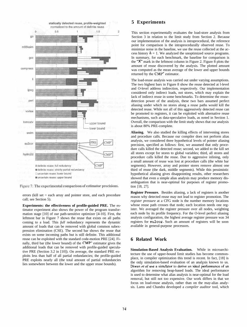
errors (kill set = each array and pointer store, and each procedurecall; see Section 5).

Experiments: the effectiveness of profile-guided PRE. The es-timator experiment also shows the power of the program transfor-mation stage [10] of our path-sensitive optimizer [4-10]. First, theleftmost bar in Figure 7 shows the reuse that exists on all pathscoming to a load. This full redundancy represents the dynamicamount of loads that can be removed with global common subex-pression elimination (CSE). The second bar shows the reuse thatexists on some incoming paths but is still definite. This additionalreuse can be exploited with the standard code-motion PRE [24]. Fi-nally, third bar (the lower bound) of the CMP” estimator gives theadditional loads that can be removed with profile-guided specula-tive PRE (Section 3.2 in [10]). On average, the standard PRE ex-ploits less than half of all partial redundancies; the profile-guidedPRE exploits nearly all (the total amount of partial redundancieslies somewhere between the lower and the upper reuse bounds).

5 Experiments

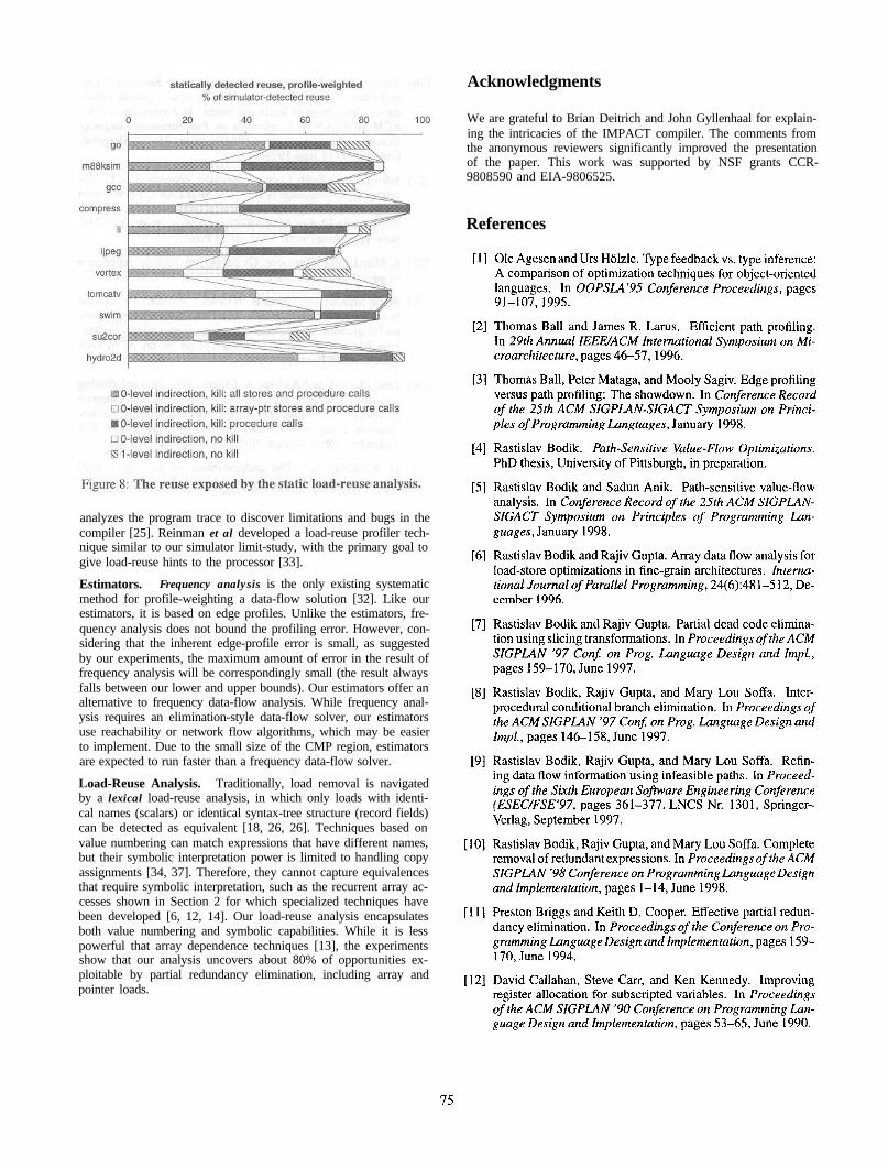
This section experimentally evaluates the load-store analysis fromSection 3 in relation to the limit study from Section 2. Becauseour implementation of the analysis is intraprocedural, the referencepoint for comparison is the intraprocedurally observed reuse. Tominimize noise in the baseline, we use the reuse collected at the ac-cess history h = 1. We analyzed the unoptimized source programs.In summary, for each benchmark, the baseline for comparison isthe “x” mark in the leftmost column in Figure 2. Figure 8 plots theamount of reuse discovered by the analysis. The plotted amountwas computed as the mean average of the lower and upper boundsreturned by the CMP’ estimator.

The load-reuse analysis was carried out under varying assumptions.The two highest bars in Figure 8 show the reuse detected at l-leveland O-level address indirection, respectively. Our implementationconsidered only indirect loads, not stores, which may explain thelack of indirect reuse in some benchmarks. To determine the reuse-detection power of the analysis, these two bars assumed perfectaliasing under which no stores along a reuse paths would kill thedetected reuse. While not all of this aggressively detected reuse canbe promoted to registers, it can be exploited with alternative reusemechanisms, such as data-speculative loads, as noted in Section 1.Overall, the comparison with the limit study shows that our analysisis about 80% PRE-complete.

Aliasing. We also studied the killing effects of intervening storesand procedure calls. Because our compiler does not perform aliasanalysis, we considered three hypothetical levels of pointer aliasingprecision, specified as follows: first, we assumed that only proce-dure calls killed the detected reuse; second, we added to the kill setall stores except for stores to global variables; third, all stores andprocedure calls killed the reuse. Due to aggressive inlining, onlya small amount of reuse was lost at procedure calls (the white barsegments). However, array and pointer stores remove almost onethird of reuse (the dark, middle segments). While this pessimistichypothetical aliasing gives disappointing results, other researchersshowed that even a simple alias analysis may produce memory dis-ambiguation that is near-optimal for purposes of register promo-tion [18, 27].

Register Pressure. Besides aliasing, a lack of registers is anotherreason why detected reuse may not lead to register promotion. Theregister pressure at a CFG node is the number memory locationswhose reuse path crosses that node; each location needs one reg-ister. We averaged the register pressure over all nodes, weightingeach node by its profile frequency. For the O-level perfect aliasinganalysis configuration, the highest average register pressure was 34registers for su2cor. Such an amount of registers will be soonavailable in general-purpose processors.

6 Related Work

Simulation-Based Analysis Evaluation. While in microarchi-tecture the use of upper-bound limit studies has become common-place, in compiler optimization this trend is recent. In fact, [18] isthe only simulation-based evaluation of an analysis known to us.

algorithm for removing heap-based loads. The ideal performanceis used to determine what alias analysis is near-optimal for the loadremoval, but still not too expensive. Our work differs in that wefocus on load-reuse analysis, rather than on the may-alias analy-sis. Lams and Chandra developed a compiler auditor tool, which

analyzes the program trace to discover limitations and bugs in thecompiler [25]. Reinman et al developed a load-reuse profiler tech-nique similar to our simulator limit-study, with the primary goal togive load-reuse hints to the processor [33].

Estimators. Frequency analysis is the only existing systematicmethod for profile-weighting a data-flow solution [32]. Like ourestimators, it is based on edge profiles. Unlike the estimators, fre-quency analysis does not bound the profiling error. However, con-sidering that the inherent edge-profile error is small, as suggestedby our experiments, the maximum amount of error in the result offrequency analysis will be correspondingly small (the result alwaysfalls between our lower and upper bounds). Our estimators offer analternative to frequency data-flow analysis. While frequency anal-ysis requires an elimination-style data-flow solver, our estimatorsuse reachability or network flow algorithms, which may be easierto implement. Due to the small size of the CMP region, estimatorsare expected to run faster than a frequency data-flow solver.

Load-Reuse Analysis. Traditionally, load removal is navigatedby a lexical load-reuse analysis, in which only loads with identi-cal names (scalars) or identical syntax-tree structure (record fields)can be detected as equivalent [18, 26, 26]. Techniques based onvalue numbering can match expressions that have different names,but their symbolic interpretation power is limited to handling copyassignments [34, 37]. Therefore, they cannot capture equivalencesthat require symbolic interpretation, such as the recurrent array ac-cesses shown in Section 2 for which specialized techniques havebeen developed [6, 12, 14]. Our load-reuse analysis encapsulatesboth value numbering and symbolic capabilities. While it is lesspowerful that array dependence techniques [13], the experimentsshow that our analysis uncovers about 80% of opportunities ex-ploitable by partial redundancy elimination, including array andpointer loads.

Acknowledgments

We are grateful to Brian Deitrich and John Gyllenhaal for explain-ing the intricacies of the IMPACT compiler. The comments fromthe anonymous reviewers significantly improved the presentationof the paper. This work was supported by NSF grants CCR-9808590 and EIA-9806525.

References

[ 131 S. Carr, K. McKinley, and C.-W. Tseng. Compiler optimizations for improving data locality. In Proceedings ofthe Sixth International Conference on Architectural Support forPro- gramming Languagesand Operating Systems (ASPWS), San Jose, CA, October 1994.

[ 141 Steve Carr and Ken Kennedy. Scalar replacement in the pres- ence of conditional control flow. Software Practice and Ex- perience, 24( 1):5 l-77, January 1994.

[ 151 Steven Carr and Ken Kennedy. Improving the ratio of memory operations to floating-point operations in loops. ACM Transactions on Programming Languages and Systems, November 1994.

[ 161 P. P. Chang, S. A. Mahlke, W. Y. Chen, N. J. Warter, and W. W. Hwu. IMPACT An architectural framework for multiple-instruction-issue processors. In Proceedings of the 18th International Symposium on Computer Architecture (ISCA), volume 19, pages 266-275, New York, NY, June 1991. ACM Press.

[ 171 Ron Cytron, Jeanne Ferrante, Barry K. Rosen, Mark N. Weg- man, and F. Kenneth Zadeck. Efficiently computing static single assignment form and the control dependence graph. ACM Transactions on Programming Languagesand Systems, 13(4):451-490, October 1991.

[18] Amer Diwan, Kathryn S. McKinley, and J. Eliot B. Moss. Type-based alias analysis. In Proceedings of the ACM SIG- PLAN’98 Conference on Programming Language Design and Implementation (PLDI), pages 106-l 17, Montreal, Canada, 17-19 June 1998. SIGPLANNotices 33(5), May 1998.

[19] E. Duesterwald, R. Gupta, and M. L. Soffa. A practical data flow framework for array reference analysis and its use in optimizations. In Proceedings of the ACM SIGPLAN ‘93 Con- ference on Programming Language Design and Implementa- tion, pages 68-77, June 1993.

[20] Benjamin Goldberg, Hans00 Kim, Vinod Kathail, and John Gyllenhaal. The trimaran compiler infrastructure for instruction level parallelism research. Technical Report http : / /www . trimaran. org, Hewlett-Packard Labora- tories, University of Illinois, NYU, 1998.

[21] R. Gupta, D. Berson, and J.Z. Fang. Resource-sensitive profile-directed dam flow analysis for code optimization. In 30th Annual IEEEJACM International Symposium on Mi- croarchitecture, pages 358-368, December 1997.

[22] W. W. Hwu, S. A. Mahlke, W. Y. Chen, P P. Chang, N. J. Warter, R. A. Bringmann, R. G. Ouellette, R. E. Hank, T. Kiy- ohara, G. E. Haab, J. G. Holm, and D. M. Lavery. The superblock: an effective technique for VLIW and superscalar compilation. In The Journal of Supercomputing. 1992.

[23] Vinod Kathail, Michael S. Schlansker, and B. Ramakrishna Rau. Hpl playdoh architecture specification: Version 1.0. Technical Report HPL-93-80, Hewlett-Packard Laborato- ries, 1994.

[24] Jens Knoop, Oliver Rtithing, and Bernhard Steffen. Optimal code motion: Theory and practice. ACM Trans. on Progr. LanguagesandSystems, 16(4):1117-1155,1994.

[25] James Larus and Satish Chandra. Using tracing and dynamic slicing to tune compilers. Technical Report TR-1174, Uni- versity of Wisconsin, 1993.

[26] Raymond Lo, Fred Chow, Robert Kennedy, Shin-Ming Liu, and Peng Tu. Register promotion by sparse partial redundancy elimination of loads and stores. In Proceedings of the ACM SIGPLAN’98 Conference on Programming Language Design and Implementation (PLDI), pages 26-37, Montreal, Canada, 17-19 June 1998.

[27] John Lu and Keith Cooper. Register promotion in C programs. In Proceedings of the ACM SIGPLAN Conference on Programming Language Design and Implementation (PLDI- 97), volume 32,5 of ACM SIGPLAN Notices, pages 308-3 19, New York, June15-18 1997. ACM Press.

[28] E. Morel and C. Renviose. Global optimization by supression of partial redundancies. CACM, 22(2):96-103,1979.

[29] Frank Mueller and David B. Whalley. Avoiding conditional branches by code replication. In ACM SIGPLAN Conference on Programming Language Design and Implementation, volume 30 of ACM SIGPZAN Notices, pages 56-66. ACM SIG- PLAN, ACM Press, June 1995.

[30] John Plevyak and Andrew A. Chien. Type directed cloning for object-oriented programs. In Eighth Annual Workshop on Languages and Compilers for Parallel Computing, Lecture Notes in Computer Science, volume 1033, pages 566-580, Columbus, Ohio, August 1995.

[31] G. Ramalingam.. The undecidability of aliasing. ACM Transactions on Programming Languages and Systems, 16(5):1467-1471, September 1994.

[32] G. Ramalingam. Data flow frequency analysis. In Proceed- ings of the ACM SIGPLAN ‘96 Conf on Progr. Language De- sign and Implementation, pages 267-277, June 1996.

[33] Glenn Reinman, Brad Calder, Dean Tullsen, Gary Tyson, and Todd Austin. Profile guided load marking for memory re- naming. Technical Report UCSD-CS98-593, University of California, San Diego, 1998.

[34] Barry K. Rosen, Mark N. Wegman, and F. Kenneth Zadeck. Global value numbers and redundant computations. In 15th Annual ACM Symposium on Principles of Programming Lan- guages, pages 12-27, San Diego, California, January 1988.

[35] A. V. S. Sastry and Roy D. C. Ju. A new algorithm for scalar register promotion based on SSA form. ACM SIGPIAN No- tices, 33(5):15-25, May 1998.

[36] Bernhard Steffen. Property oriented expansion. In Proc. Int. Static Analysis Symposium (SAS’96), volume 1145 of LiVCS, pages 22-41, Germany, September 1996. Springer.

[37] Bernhard Steffen, Jens Knoop, and 0. Rtithing. The value flow graph: A program representation for optimal program transformations. In Proceedings of the 3rd European Sympo- sium on Programming (ESOP’90), volume 432, pages 389- 405, Denmark, May 1990.

[38] Youfeng Wu. Conflict Ratio Profiling for Memory Refer- ences. Technical Report MRL Compiler Technical Report 96012, Intel Corp., 1996.

[39] Cliff Young and Michael D. Smith Improving the accuracy of static branch prediction using branch correlation. In Proceed- ings of the Sixth International Conference on Architectural Supportfor Programming Languagesand Operating Systems, pages 232-241, San Jose, California, October 4-7, 1994.

76

Documents

Load-Reuse Analysis: Design and Evaluation