Title: Evaluation of System Effects and Structural Load

AN ABSTRACT OF THE THESIS OF

Kenneth G. Martin for the degree of Master of Science in Civil Engineering and

Wood Science presented on January 29, 2010.

Title: Evaluation of System Effects and Structural Load Paths in a Wood-Framed

Structure.

Abstract approved:

Rakesh Gupta

The objective of this project was to develop an analytical model of a light-

framed wood structure using a prevalent structural analysis computer program in

order to evaluate system effects and define load paths within the structure,

especially under extreme wind events. Simplified modeling techniques and

material definitions were developed and used throughout the analysis.

A three dimensional 30-ft by 40-ft building was modeled using SAP2000.

The building had a gable roof system comprised of Fink trusses. Wall and roof

sheathing was modeled using SAP’s built-in thick shell element. Conventional

light-frame construction practices were assumed, and the model was linear with all

joints considered to be either pinned or rigid. Also, the effect of edge nail spacing

of the wall sheathing was incorporated by way of a novel correlation procedure

which eliminates the need to represent each nail individually. Instead, a single

sheathing element represented each wall and property modifiers were assigned to

that wall element based on the nailing schedule. The NDS 3-term shear wall

equation was used to derive the correlation procedure and the correlated model was

compared to full-scale testing results with good agreement.

The computer model was validated against both two and three dimensional

experimental studies (in-plane and out-of-plane). Once validated it was subjected

to uniform loads to gain insight into its uplift behavior. Uniform uplift pressure

was applied to the roof, and vertical foundation reactions were evaluated. In this

phase of the investigation, the building geometry was altered in several different

ways to explore the effect of these variations. Next, the model was subjected to

several uplift loading scenarios corresponding to worst-case simulated hurricane

events. With these inputs, the same uplift reaction profiles were generated.

Finally, for comparison the model was loaded using the “Component and

Cladding” pressures determined at a comparable wind speed, as given by ASCE

7-05 (lateral and uplift).

The ASCE 7-05 uplift pressures were found to adequately encompass the

range of uplift reactions that can be expected from a severe wind event such as a

hurricane. Also, the analytical model developed in this study inherently takes into

account system effects. Consequently, it was observed that ASCE 7-05

“Component and Cladding” pressures satisfactorily captured the building’s uplift

response at the foundation level without the use of “Main Wind Force-Resisting

System” loads. Additionally, it was noted that the manner in which the walls of the

structure distribute roof-level loads to the foundation depends on the edge nailing

of the wall sheathing. Finally, the effects of variations in the building geometry

were explored and notable results include the presence of a door in one of the walls.

It was revealed that the addition of a door to any wall results in a loss of load-

carrying capacity for the entire wall. Moreover, the wall opposite the one with the

door can also be significantly affected depending on the orientation of the trusses.

In general, it was determined that complex, three-dimensional building

responses can be adequately characterized using the practical and effective

modeling procedures developed in this study. The same modeling process can be

readily applied in industry for similar light-framed wood structures.

©Copyright by Kenneth G. Martin

January 29, 2010

All Rights Reserved

EVALUATION OF SYSTEM EFFECTS AND STRUCTURAL LOAD PATHS

IN A WOOD-FRAMED STRUCTURE

by

Kenneth G. Martin

A THESIS

submitted to

Oregon State University

in partial fulfillment of

the requirements for the

degree of

Master of Science

Presented January 29, 2010

Commencement June 2010

Master of Science thesis of Kenneth G. Martin presented on January 29, 2010 APPROVED: Major Professor Representing Wood Science and Civil Engineering Head of the Department of Wood Science and Engineering Head of the School of Civil and Construction Engineering Dean of the Graduate School I understand that my thesis will become part of the permanent collection of Oregon State University libraries. My signature below authorizes release of my thesis to any reader upon request.

Kenneth G. Martin, Author

ACKNOWLEDGEMENTS

I would like to thank the following people and organizations for their help

and support:

Dr. Rakesh Gupta – Professor, Oregon State University

Dr. Tom Miller – Associate Professor, Oregon State University

Dr. David Prevatt – Assistant Professor, University of Florida

Peter Datin – Ph.D. candidate, University of Florida

Akwasi Mensah – M.S. candidate, University of Florida

Dr. John van de Lindt – Associate Professor, Colorado State University

Faculty and staff in the Wood Science and Engineering department, OSU

Faculty and staff in the Civil and Construction Engineering department,

OSU

Beth and Cora Martin – Loving wife and daughter

NSF award no. CMMI 0800023

Partial funding provided by USDA Center for Wood Utilization research

grant

TABLE OF CONTENTS Page INTRODUCTION ............................................................................................. 1 MATERIALS AND METHODS................................................................... 8 GENERAL .................................................................................................. 8

MODELING ............................................................................................... 9

Shell Element Behavior .................................................................. 9

Connectivity .................................................................................. 11

Stiffness of Hold-downs and Anchor Bolts .................................. 11

Material Properties ........................................................................ 12

RESEARCH METHODS ......................................................................... 14

Verification / Validation ............................................................... 14

Load Cases .................................................................................... 14

Geometry Scenarios ...................................................................... 15

RESULTS AND DISCUSSION................................................................... 16

MODEL VALIDATION........................................................................... 16

CORRELATION MODEL FOR NAILING SCHEDULE OF SHEATHING............................................................................................ 16 UNIFORM UPLIFT PRESSURE............................................................. 18

Standard Geometry (Control Case)............................................... 18

Effect of Edge Nailing .................................................................. 21

Extended Building (30-ft x 92-ft) ................................................. 23

TABLE OF CONTENTS (Continued)

Page RESULTS AND DISCUSSION (Continued)

UNIFORM UPLIFT PRESSURE (Continued)

Effect of Door Openings ............................................................... 24

Gable Wall Missing (Three-sided structure)................................. 32

Effect of Roof Blocking ................................................................ 33

Effect of Overhang Construction (Ladder vs. Outlooker) ............ 33

Effect of Anchor Bolt Spacing (4-ft vs. 6-ft) ................................ 34

Effect of Anchor Bolts Missing .................................................... 34

SIMULATED HURRICANE UPLIFT PRESSURES.............................. 35

ASCE 7-05 PRESSURES ......................................................................... 40

COMPARISONS ...................................................................................... 44

ROOF SHEATHING UPLIFT.................................................................. 47

CONCLUSIONS AND RECOMMENDATIONS .................................. 49

SUGGESTIONS FOR FURTHER RESEARCH ..................................... 51

PRACTICAL ADVICE ............................................................................ 53

BIBLIOGRAPHY............................................................................................ 55

APPENDICES .................................................................................................. 60

LIST OF FIGURES Figure Page 1. SAP model of the index building.................................................................... 9

2. Meshing of the wall sheathing in the gable ends.......................................... 11

3. Reaction profile for the gable wall, uniform uplift pressure ........................ 19

4. Load accumulation in the gable end below the ridge of the roof ................. 19

5. Reaction profile for the side wall, uniform uplift pressure........................... 20

6. Effect of edge nailing for the gable wall, uniform uplift pressure................ 22

7. Effect of edge nailing for the side wall, uniform uplift pressure.................. 22

8. Load distribution within the roof of the extended building when subjected to uniform uplift............................................................................ 24 9. Reaction profile for the end walls with door in center of near-side gable wall...................................................................................................... 25 10. Reaction profile for the side walls with door in center of near-side gable wall...................................................................................................... 26 11. Reaction profile for the side walls when a door is centered in the near side wall ................................................................................................ 27 12. Reaction profile for the side walls when a door is located off-center in the near side wall ...................................................................................... 30 13. Reaction profile for the gable walls when a door is located off-center in the near side wall ...................................................................................... 31 14. Wind tunnel pressures, load case 1 – maximum uplift at the corner of the roof.......................................................................................................... 36 15. Wind tunnel pressures, load case 2 – local maxima over entire roof ........... 38 16. Wind tunnel pressures, load case 3 – maximum pressure at the ridge ......... 39

LIST OF FIGURES (CONTINUED) Figure Page 17. Side wall reaction profile with ASCE 7-05 lateral pressures acting alone.............................................................................................................. 41 18. System effects within the truss assembly due to lateral loads ...................... 41 19. Gable wall reaction profile with ASCE 7-05 lateral pressures acting alone.............................................................................................................. 43 20. Comparison between uplift reactions using ASCE 7-05 and those predicted by the simulated hurricane events................................................. 44

LIST OF TABLES Table Page 1. Spring stiffness used to model the anchor bolts and hold-downs................. 12 2. Elastic isotropic material properties used in the SAP model........................ 12 3. Elastic orthotropic material properties used in the SAP model .................... 13 4. Correlation between nailing schedule and the shear modulus G12 of the shell element in SAP............................................................................... 17

LIST OF APPENDICES Appendix Page A Construction Details of the Index Building .................................. 61

B Modeling Techniques.................................................................... 68

C Validating the Model .................................................................... 85

D 3D Verification – Load Sharing Study.......................................... 97

E Correlation to Nailing Schedule of Sheathing ............................ 109

F Influence Functions – Contour Plots........................................... 119

G Uniform Uplift Pressure Load Cases .......................................... 126

H Simulated Hurricane Pressures ................................................... 147

I ASCE 7-05 Load Cases............................................................... 156

J Roof Sheathing Uplift Calculation.............................................. 166

K Literature Review........................................................................ 171

LIST OF APPENDIX FIGURES Figure Page A-1 SAP model of the index building – frame members shown with sheathing ................................................................................................... 63 A-2 SAP model of the index building showing the meshing of the sheathing (represented by shell elements)................................................. 63 A-3 SAP model of the index building showing the springs which represent anchor bolts and hold-downs .................................................................... 64 A-4 SAP model of the index building – extruded view of framing members (sheathing not shown for clarity) .............................................................. 64 A-5 SAP model of the index building – view looking down ........................... 65 A-6 Interior section view of the index building in SAP................................... 65 A-7 Framing plan, sheet 1 of 4 – Overall plot plan.......................................... 66 A-8 Framing plan, sheet 2 of 4 – Gable wall details........................................ 66 A-9 Framing plan, sheet 3 of 4, Side wall details ............................................ 67 A-10 Framing plan, sheet 4 of 4 – Truss detail .................................................. 67 B-1 Analog used in SAP2000 .......................................................................... 68 B-2 Typical wall detail..................................................................................... 70 B-3 Typical roof sheathing detail..................................................................... 71 B-4 Meshing of shell elements based on maximum size ................................. 72 B-5 Meshing of shell elements based on points and lines in a specified meshing group........................................................................................... 74 B-6 Connectivity of the trusses – mixture of pinned and rigid joints .............. 75 B-7 Detail of the truss heel showing the offset between heel joint and connection to the top plate ........................................................................ 75

LIST OF APPENDIX FIGURES (CONTINUED) Figure Page B-8 All connections within the wall are considered to be pinned.................... 76 B-9 Orientation of axes for anchor bolts and hold-down devices.................... 77 B-10 Inboard and outboard vertical deflection measurements for a typical partially anchored wall.............................................................................. 79 B-11 Stiffness in the vertical direction for a typical partially anchored wall............................................................................................................ 79 C-1 SAP model for the 2D verification ........................................................... 86 D-1 Truss 1 loaded individually....................................................................... 97 D-2 Truss 2 loaded individually....................................................................... 98 D-3 Truss 3 loaded individually....................................................................... 98 D-4 Truss 4 loaded individually....................................................................... 99 D-5 Truss 5 loaded individually....................................................................... 99 D-6 Truss 6 loaded individually..................................................................... 100 D-7 Truss 7 loaded individually..................................................................... 100 D-8 Truss 8 loaded individually..................................................................... 101 D-9 Truss 9 loaded individually..................................................................... 101 D-10 Truss 1 loaded individually..................................................................... 102 D-11 Truss 2 loaded individually..................................................................... 103 D-12 Truss 3 loaded individually..................................................................... 103 D-13 Truss 4 loaded individually..................................................................... 104 D-14 Truss 5 loaded individually..................................................................... 104

LIST OF APPENDIX FIGURES (CONTINUED) Figure Page D-15 Truss 6 loaded individually..................................................................... 105 D-16 Truss 7 loaded individually..................................................................... 105 D-17 Truss 8 loaded individually..................................................................... 106 D-18 Truss 9 loaded individually..................................................................... 106 D-19 Load sharing when all trusses are loaded simultaneously ...................... 107 D-20 Deflection sharing when all trusses are loaded simultaneously.............. 108 E-1 The depicted correlation procedure was repeated for each nail spacing ............................................................................................. 110 E-2 OSB-only shear wall tests – 11 total walls ............................................. 115 E-3 Comparison to correlated SAP model at 4-in o.c. edge nailing .............. 115 E-4 Average stiffness for each type of wall study ......................................... 116 E-5 Comparison of the correlated SAP model to the individual averages .... 116 E-6 Combined average of the OSB-only walls compared to the correlated SAP model ............................................................................. 117 E-7 Include the OSB+GWB walls for a total comparison (22 walls)............ 117 E-8 Percent error in predicted deflection as the length of the shear wall increases .......................................................................................... 118 F-1 Construction of the 1/3 scale model at the University of Florida ........... 121 F-2 Construction of the 1/3 scale model at the University of Florida ........... 121 F-3 Construction of the 1/3 scale model at the University of Florida ........... 122 F-4 Construction of the 1/3 scale model at the University of Florida ........... 122

LIST OF APPENDIX FIGURES (CONTINUED) Figure Page G-14 Uniform pressure, effect of anchor bolt missing in the side wall ........... 140 G-15 Uniform pressure, effect of anchor bolt missing in the gable wall ......... 141 G-16 Deflected shape – standard geometry (control case)............................... 142 G-17 Deflected shape – extended building ...................................................... 142 G-18 Deflected shape – door in gable wall ...................................................... 143 G-19 Deflected shape – door in side wall (centered) ....................................... 143 G-20 Deflected shape – door in side wall (not centered) ................................. 144 G-21 Deflected shape – doors centered in both walls ...................................... 144 G-22 Deflected shape – gable wall missing ..................................................... 145 G-23 Deflected shape – anchor bolt missing in gable wall.............................. 145 G-24 Deflected shape – anchor bolt missing in side wall ................................ 146 H-1 Wind tunnel arrangement for 1:50 scale model of index building in suburban terrain .................................................................................. 147 H-2 1:50 scale model of the index building ................................................... 148 H-3 Wind tunnel pressures, load case 1 ......................................................... 150 H-4 Wind tunnel pressures, load case 2 ......................................................... 151 H-5 Wind tunnel pressures, load case 3 ......................................................... 152 H-6 Deflected shape – load case 1 ................................................................. 153 H-7 Deflected shape – load case 1 (view looking down)............................... 153 H-8 Deflected shape – load case 2 ................................................................. 154

LIST OF APPENDIX FIGURES (CONTINUED) Figure Page H-9 Deflected shape – load case 2 (view looking down)............................... 154 H-10 Deflected shape – load case 3 ................................................................. 155 H-11 Deflected shape – load case 3 (view looking down)............................... 155 I-1 ASCE 7-05 pressures, uplift loads acting alone...................................... 159 I-2 ASCE 7-05 pressures, lateral loads acting alone .................................... 160 I-3 ASCE 7-05 pressures, lateral plus uplift loads ....................................... 161 I-4 ASCE 7-05 uplift response compared to the wind tunnel simulations .............................................................................................. 162 I-5 ASCE 7-05 uplift response compared to the wind tunnel simulations .............................................................................................. 163 I-6 Deflected shape – ASCE 7-05 uplift loads acting alone ......................... 164 I-7 Deflected shape – ASCE 7-05 lateral loads acting alone........................ 164 I-8 Deflected shape – ASCE 7-05 lateral + uplift loads ............................... 165 J-1 Typical roof sheathing panel with 6-inch edge nailing and 12-inch field nailing ............................................................................................. 169

LIST OF APPENDIX FIGURES (CONTINUED) Figure Page F-5 The completed 1/3 scale model at the University of Florida .................. 123 F-6 The pneumatic actuator applied uplift lads normal to the roof ............... 123 F-7 Uplift loads were applied consecutively at each green dot using a pneumatic actuator...................................................................... 124 F-8 Load cell placement in the 1/3 scale wood frame house......................... 124 F-9 Comparison between influence functions determined (a) experimentally and (b) analytically using SAP ................................. 125 G-1 Uniform pressure, standard building geometry....................................... 127 G-2 Uniform pressure, standard building – effect of nailing schedule .......... 128 G-3 Uniform pressure, extended building...................................................... 129 G-4 Comparison between the standard and the extended building ................ 130 G-5 Uniform pressure, door in end wall......................................................... 131 G-6 Uniform pressure, door in side wall........................................................ 132 G-7 Uniform pressure, door in side wall – effect of header depth and ceiling ............................................................................................... 133 G-8 Uniform pressure, door in side wall – not centered ................................ 134 G-9 Uniform pressure, doors centered in both walls...................................... 135 G-10 Uniform pressure, gable wall missing..................................................... 136 G-11 Uniform pressure, blocked vs. unblocked roof assembly ....................... 137 G-12 Uniform pressure, effect of changing the overhang framing style.......... 138 G-13 Uniform pressure, effect of anchor bolt spacing (4-ft vs. 6-ft) ............... 139

LIST OF APPENDIX TABLES Table Page B-1 Comparison of MOE values for determining the load-slip modulus ........ 80 B-2 Spring stiffness used to model the anchor bolts and hold-downs ............. 80 B-3 Elastic isotropic material properties used in the SAP model .................... 81 B-4 Elastic orthotropic material properties used in the SAP model ................ 82 C-1 2D verification – deflection comparison for 6:12 slope trusses tested to their design load.......................................................................... 87 C-2 3D verification – Absolute percent differences in load sharing when each truss is loaded individually ..................................................... 91 C-3 3D verification – Average percent differences in deflection sharing when each truss is loaded individually ..................................................... 91 C-4 3D verification – Percent differences in load and deflection sharing when all trusses are loaded simultaneously .............................................. 92 E-1 Apparent stiffness for 7/16” OSB and computed deflections using the SDPWS 3-term shear wall equation at a load value of 3,000 lbs.............................................................................................. 110 E-2 Correlation between nailing schedule and the shear modulus G12 of the shell element in SAP..................................................................... 111 I-1 Applied pressures using ASCE 7-05 for “Components and Cladding” ................................................................................................ 158

EVALUATION OF SYSTEM EFFECTS AND STRUCTURAL LOAD PATHS IN A WOOD-FRAMED STRUCTURE

INTRODUCTION

A successful structural design, in its most basic form, must ensure that

buildings are capable of supporting loads and performing their intended functions.

To do so, engineers employ a process that is typically considered to include only

two major phases: 1) the determination of loads acting on a structure, followed by

2) an analysis of the individual members to ensure they can withstand the loads.

Too often it is assumed that these phases can be performed separately so long as the

end result shows that member capacity exceeds the demand. However, there are

two very fundamental concepts that must also be integrated into structural design,

yet are often overlooked. The first concept is the need for a continuous load path.

Forces originating at any point in the structure must have a route by which they can

be transmitted through the structure and safely to the ground. In this sense, it is

best to consider buildings not as mere assemblies that simply support loads, but

rather as complex systems that transmit loads. Second, designers must consider

system effects that exist within the structure. Today’s buildings are so complex

that individual members inherently share load with their neighbors, yet these

interactions are seldom incorporated into structural evaluations. This is perhaps

due to the fact that there is generally no practical manner by which to address

system effects. In fact, present convention simply addresses load sharing by way of

conservative factors applied to design values, such as the repetitive member factor

2

used in the NDS code (AF&PA 2005a) which accounts for both load sharing and

partial composite action.

LOAD PATHS

In so far as load paths are concerned, it has been documented that although

the basic topic is covered in most structural engineering texts, the discussions

provided are usually not comprehensive enough to provide an understanding of the

principles involved (Taly 2003). In fact, one of the nation’s preeminent manuals on

wood frame construction makes the following statement in its general provisions:

A continuous load path shall be provided to transfer all lateral and vertical loads from the roof, wall, and floor systems to the foundation. (AF&PA 2001)

However, it does not provide any additional details on how to do so. The

commentary to the manual is of no help either – it actually skips over this sub-

section, addressing the topics before and after it but providing no further

clarification on the topic of load paths. To complicate matters, engineers and

designers must account for the fact that load paths in a structure are different for

vertical loads compared to lateral loads, and they vary from one structure to

another. Yet, despite these hurdles, it is nonetheless essential that load paths be

well understood and evaluated in performing any structural analysis. Experience

has shown that failure to do so leads to significant damage and even collapse (Taly

2003). History validates this notion. Albeit unfortunate, devastating events such as

natural disasters tend to highlight both the gross oversights as well as the subtle

misunderstandings of load paths. For example, in the aftermath of hurricane

3

Katrina, damage assessment teams observed widespread damage and significant

patterns of structural failure. Above all else, these teams emphasized a lack of load

path, especially due to uplift, as one of the prevalent failure mechanisms observed

(van de Lindt et al. 2007).

TYPE OF LOADING

The need to identify and understand load paths is clear. This much is

known. Implicit in this statement though is the assumption that the loads are also

known, which is not always the case. As mentioned, the type of loading can vary.

Loads can originate from any number of sources including snow, wind,

earthquakes, personnel, and even the weight of the structure itself. Each of these

load sources has the potential to cause a structural failure or, at the very least,

render the building unfit to perform its intended purpose. Alongside this failure,

there is a cost that is incurred to repair or replace the structure. If the prevalence

for failure and the associated costs are considered as criteria to rank the

aforementioned loads, wind tops the list. Wolfe (1998) gives further details about

this fact, stating:

In the U.S., wind is the most common – and the most costly – cause of damage to buildings. Over a seven year period from 1986 to 1993 extreme wind damage cost $41 billion in insured catastrophe losses as compared to $6.8 billion for all other natural hazards combined.

This precedent was further endorsed with Hurricane Katrina, which made landfall

towards the middle of the hurricane season in late August of 2005. Katrina was by

far the mot costly hurricane – and disaster – in U.S. history (van de Lindt et al.

2007).

4

The term “extreme wind events” is not limited to hurricanes though.

Included in this subset of natural hazard events are also tornadoes and severe

storms. Taken as a whole, the losses from these extreme wind events continue to

increase, doubling approximately every 5-10 years (Davenport 2002).

Interestingly, hurricanes wreak the most havoc. They normally cause twice the

damage of tornadoes in any one year and over 160 times the damage of severe

winds (Wolfe 1998). One reason for this fact is that tornadoes usually affect a

smaller land area than hurricanes. More critical though is the fact that winds

associated with hurricanes are accompanied by large amounts of rain. Wind-

driven rain saturates insulation and ceiling drywall, causing it to collapse. Damage

in these cases is extensive and costly to repair.

CONSTRUCTION PRACTICES

Improvements to light-frame residential construction practices were made

and subsequently adopted following Hurricane Andrew in 1994. However, 90% of

the homes in the U.S. were built prior to the adoption of these provisions (US

Census Bureau 2003). As a result, these structures remain vulnerable to the

damaging effects of hurricane winds. Also, newly constructed buildings can still

find themselves at the mercy of wind loads, despite being constructed after the new

code provisions. Although evidence has proven that recently built homes fair better

than older homes, this only holds true when the design codes and guidelines are

followed (van de Lindt et al. 2007). Regrettably, many of the prescriptive

5

recommendations are either misunderstood or incorrectly applied (APA 1997). The

damage assessment teams after Hurricane Katrina observed this firsthand, noting:

Builders and inspectors in the Mississippi Gulf Coast region appear to be familiar with conventional construction provisions. However, these provisions were used erroneously in a high wind region. (van de Lindt et al. 2007)

Consequently, buildings both old and new are susceptible to failures as a result of

exposure to high wind loads. Therefore, it is critical to gain a deeper understanding

of hurricane wind loads and their effect on light-frame wood structures.

SYSTEM EFFECTS

Previous research has been conducted in the realm of wood-frame structures

exposed to wind loads, but it has stopped short of fully addressing all of the

mechanisms that are at play within these complex systems, especially in uplift

scenarios. For example, much of the research has concentrated towards specific

components within the structure, such as roof or wall sheathing (Sutt 2000, Hill et

al. 2009), or towards one particular type of connection, e.g. roof-to-wall (Reed et

al. 1997, Riley and Sadek 2003). Very little work has been done to address system

effects as a whole in full-size buildings. Fortunately, this shortfall can be overcome

by using an analytical tool, such as a modern structural analysis computer program,

which directly incorporates system interactions.

ANALYTICAL MODELING

Naturally, the use of modern computers has made the bookkeeping and

computational aspects of structural analyses much easier; however, the major

6

market for these tools has been in the realm of steel and concrete design. Wood

structures have received far less attention in so far as modern computer programs

are concerned. Yet tools that are widely used in academia and in practice, such as

SAP2000, possess significant potential to the wood industry if manipulated to

predict the response of wood-framed systems. With this in mind, the major thrust

of this research has focused on the development of simple, yet accurate material

assignments and property correlations to customize SAP2000 for use in three-

dimensional wood structures. Considerable efforts were made to use built-in

features of SAP2000 in conjunction with simple modeling techniques to capture

complex structural responses (e.g. system effects, effect of nailing schedule, etc.).

OBJECTIVES

The following tasks represent the overall objectives of this study. It is

worth noting that throughout this research, one goal has been kept at the forefront

as each task was confronted: the initiative to address very complex structural

behaviors using only the most pragmatic modeling techniques possible. In this

fashion, the hope is that wood engineers and designers can use these same methods

in industry to readily and accurately predict the behavior of similar wood

structures. Specific goals were:

1. Develop a practical 3D computer model of a full-size light-frame wood

structure.

2. Develop a practical representation of the sheathing nailing schedule to

be incorporated into the computer model.

7

3. Evaluate critical load paths and system effects for different building

geometries under various loading scenarios.

8

MATERIALS AND METHODS

GENERAL

An analytical model of a light-frame wood structure was developed and

validated. Then, to better understand the behavior of the model in the presence of

uplift loads, a uniform uplift pressure was applied to the roof sheathing. Several

scenarios (e.g. changing the anchor bolt spacing, adding a door to one of the walls,

etc.) were considered while the structure was subjected to this uniform pressure.

Next, simulated hurricane uplift loads were applied to the model. Finally, the

structure was subjected to ASCE 7-05 pressures. For direct comparison, the

reaction profile of the structure under these code assigned loads was compared to

the response of the building under the simulated hurricane loads.

The analytical model of the index building was developed using SAP2000

(Figure 1). This commercial software package – developed by Computers and

Structures, Inc. based in Berkeley, California – is widely used in academia and

industry. The model is comprised entirely of pinned or rigid connections, and all

materials are assumed to behave within the elastic range. Non-linearity is not

incorporated into this study. Studs and truss members are represented using frame

elements with isotropic material properties. Wall and roof sheathing are modeled

using the thick shell element with orthotropic material properties. Anchorage

devices are represented by grounded springs (Computers and Structures, 2008).

The footprint of the index building is approximately 30-ft x 40-ft with

overhangs on all sides. The gable roof has a 4:12 slope. Studs are spaced 16-

9

inches on center and trusses are 24-inches on center. There are no interior

partitions (see Figure 1). Specific construction features and detailed framing plans

of the index building can be found in Appendix A.

Figure 1. SAP model of the index building (exterior sheathing not shown for clarity).

MODELING

Shell Element Behavior

The roof sheathing (1/2” plywood) and wall sheathing (7/16” OSB) were

modeled using SAP’s thick shell element. Each wall and roof area was defined in

the modeling environment using one shell element. That is, individual sheets of 4-

ft x 8-ft plywood/OSB were not modeled. For example, the entire side wall is

represented by just one shell element in SAP. Likewise, each side of the roof is

comprised of a single shell element as well. It should be noted that SAP ultimately

divides each single modeling shell element into multiple analysis shell elements in

10

a process known as meshing. The user can choose how the mesh is defined

(Appendix B), and SAP also allows the user to inspect the mesh of each shell

element by viewing the internal “analysis model” (Figure 2). However, in the

modeling environment – where the walls and roof structure are defined and

manipulated – only individual shell elements were used to represented each

wall/roof section. By choosing to model the sheathing in this manner, it is assumed

that the actual 4-ft x 8-ft sheathing panels transfer load and moment continuously

across their joints. This practical assumption can be judged by examining the wall

and roof systems in greater detail. In wall systems, blocking along all panel edges

and high nailing density contribute to the validity of the assumption. In roof

systems, the assumption of continuity across the joints is drawn from four sources:

(1) staggered joints along truss lines, (2) edge nail spacing of 6-inch or less along

truss lines, (3) unblocked panel edges have nails within 3/8-inch from the edge, and

(4) “H-clips” are located in the bays between trusses. Appendix B provides further

details and accompanying figures related to this discussion (Figures B-2 and B-3).

Once the shell element has been defined in the model, it is meshed into

multiple analysis elements to ensure proper interaction with the framing members.

For simplicity, the automatic meshing option feature was used as shown in

Figure 2. Additional details related to the meshing of the shell element are

provided in Appendix B.

11

Figure 2. Meshing of the wall sheathing in the gable ends. “General divide” was used for the triangular region above the top plate of the wall.

Connectivity

All joints in the SAP model are either pinned or rigid. Doing so provides

convenience and ease of modeling by eliminating the need for semi-rigid

connections, non-linear “link” elements, and complicated spring systems to

represent joint behavior. For additional details, see Appendix B.

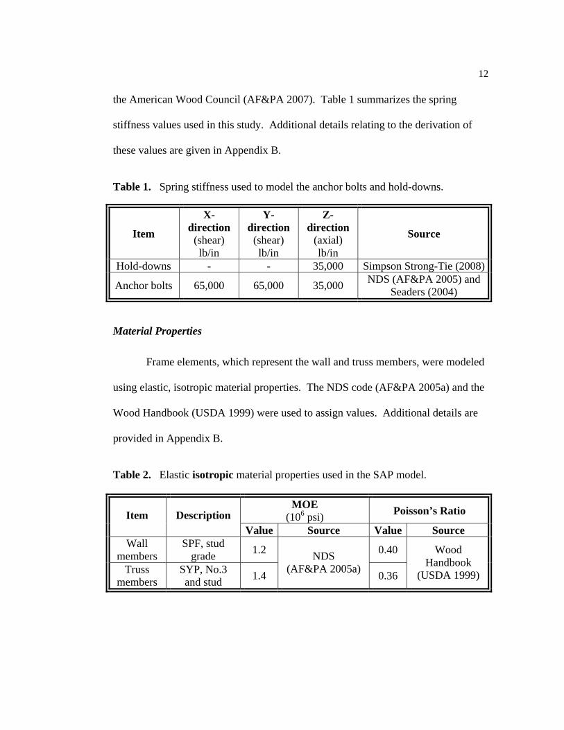
Stiffness of Hold-downs and Anchor Bolts

The axial stiffness of the hold-down device is listed by the manufacturer

(Simpson Strong-Tie, 2008). The most common type of connector, the HDU2, was

selected. The published axial stiffness of this connector is 35,000 lb/in. This value

takes into account fastener slip, hold-down elongation, and bolt elongation. The

axial stiffness of the anchor bolts, on the other hand, was determined using data

from a previous research effort (Seaders 2004). The shear stiffness of the anchor

bolts in the X and Y-direction was determined using a procedure recommended by

Mesh based on points and lines (“General divide”)

16” x 16” mesh for walls (“Max size”)

12

the American Wood Council (AF&PA 2007). Table 1 summarizes the spring

stiffness values used in this study. Additional details relating to the derivation of

these values are given in Appendix B.

Table 1. Spring stiffness used to model the anchor bolts and hold-downs.

Item

X-direction

(shear) lb/in

Y-direction

(shear) lb/in

Z-direction

(axial) lb/in

Source

Hold-downs - - 35,000 Simpson Strong-Tie (2008)

Anchor bolts 65,000 65,000 35,000 NDS (AF&PA 2005) and Seaders (2004)

Material Properties

Frame elements, which represent the wall and truss members, were modeled

using elastic, isotropic material properties. The NDS code (AF&PA 2005a) and the

Wood Handbook (USDA 1999) were used to assign values. Additional details are

provided in Appendix B.

Table 2. Elastic isotropic material properties used in the SAP model.

MOE (106 psi) Poisson’s Ratio Item Description

Value Source Value Source Wall

members SPF, stud

grade 1.2 0.40

Truss members

SYP, No.3 and stud 1.4

NDS (AF&PA 2005a) 0.36

Wood Handbook

(USDA 1999)

13

Wall and roof sheathing were each modeled using SAP’s thick shell

element. Orthotropic, elastic material properties were then assigned. Nine

constants are needed to describe the behavior of these materials, although only the

values shown in bold (Table 3) affect the response of the model. Further

explanation of this point is provided in Appendix B. The values given in Tables 2

and 3 were used for all wall and roof sections in the index building with one

exception. The shear modulus, G12, of the wall sheathing was modified using the

correlation procedure as described in the “Results and Discussion” section and in

Appendix E. Table 4 provides the correlated shear modulus values for the wall

sheathing.

Table 3. Elastic orthotropic material properties used in the SAP model.

Description MOE (105 psi)

Shear Modulus (105 psi)

Poisson’s Ratio4

Item Type E1 E2 E3 G12 G13 G23 µ12 µ13 µ23 Wall

sheathing1,2 7/16” OSB 7.4 2.3 2.3 1.2 1.2 1.2 0.08 0.08 0.08

Roof sheathing3

½” Plywood 19 2.9 2.9 1.5 1.5 1.5 0.08 0.08 0.08

1 MOE and shear modulus values from Doudak (2005) 2 Shear modulus values subject to the correlation procedure (Table 4) 3 MOE and shear modulus values from Wolfe and McCarthy (1989) and Kasal (1992) 4 Poisson’s ratio from Kasal (1992)

14

RESEARCH METHODS

The following steps were used to validate and load the model. The

geometry modifications listed were explored for the uniform uplift pressure load

case only.

Verification / Validation

The following validation procedures were explored in support of this

research effort. The studies from literature which were used for comparison are

noted. Further information pertaining to each scenario is provided in the

appendices also noted.

1. Two-dimensional individual truss behavior – Wolfe et al. (1986) –

Appendix C

2. Three-dimensional roof assembly behavior – Wolfe and McCarthy (1989) –

Appendices C and D

3. Two-dimensional shear wall behavior – Langlois (2002), Lebeda (2002),

and Sinha (2007) – Appendices C and E

4. Three-dimensional influence functions of the entire building – Datin (2009)

– Appendices C and F

Load Cases

The following load cases were explored in support of this research effort.

Further information pertaining to each scenario is provided in the appendices noted.

1. Uniform uplift pressure – Appendix G

2. Simulated hurricane uplift pressures – Appendix H

15

a. Load case 1 – Absolute maximum uplift at the corner of the roof

b. Load case 2 – Local maxima over entire roof

c. Load case 3 – Absolute maximum uplift at the ridge of the roof

3. ASCE 7-05 pressures – Appendix I

a. Uplift acting alone

b. Lateral forces acting alone

c. Combination of uplift and lateral forces

Geometry Scenarios

The following geometry variations were explored for the first load case

noted above (uniform uplift pressure). The standard building geometry was used

for the simulated hurricane uplift and the ASCE 7-05 pressures.

1. Standard building (control case)

2. Changing the edge nailing of the wall sheathing

3. Adding length to the building

4. Presence of doors in each wall

5. Gable wall missing (three-sided structure)

6. Presence of roof blocking

7. Different overhang construction (ladder vs. outlooker)

8. Varying the anchor bolt spacing

9. Removing anchor bolts at key locations

16

RESULTS AND DISCUSSION

MODEL VALIDATION

A four-step validation procedure, incorporating both 2D and 3D behavior,

was used to ensure the accuracy of the SAP2000 modeling techniques. First, a 2D

individual truss comparison was conducted against Wolfe et al. (1986) in order to

verify the assumptions of pinned/rigid joint connectivity within the truss. Next, a

3D roof assembly (Wolfe and McCarthy, 1989) verified the load sharing response

of the model. Third, a 2D investigation using multiple sources – Langlois (2002),

Lebeda (2002), and Sinha (2007) – was performed to establish the validity of the

shear wall behavior. Finally, the model of the index building itself was validated

against a 1/3 scale prototype tested by researchers at the University of Florida

(Datin 2009). The results of this multipart verification process showed that the

SAP2000 computer model and the simplified techniques used in its creation

adequately characterize the structural responses witnessed by physical testing.

Details pertaining to each verification step are provided in Appendix C.

CORRELATION MODEL FOR NAILING SCHEDULE OF SHEATHING

One of the primary objectives of the present study was to develop a

practical means to incorporate the effect of edge nailing into the SAP model.

Previous researchers have modeled fasteners individually using a set of “zero-

length link elements” for each nail. If the nailing schedule is changed, the model

must be revised one nail at a time. Although this arrangement directly takes into

17

account the actual number of nails in the system, the process can be laborious. This

may seem reasonable for sub-assembly models like segments of a shear wall, but

for full-size 3D complex structures it is simply not feasible.

Table 4 presents the results of the correlation study. These values relate the

change in stiffness resulting from a variation in the edge nailing to the shear

modulus for the shell element, G12, of the wall sheathing in SAP. It should be

noted that the extent to which edge nailing affects diaphragm or shear wall stiffness

is dependent on the presence of blocking. Unblocked systems, such as residential

roof systems, are relatively unaffected by changes in the edge nailing. On the other

hand, blocked systems, such as residential wall systems (assuming the typical

practice of placing OSB panels vertically), do respond to changes in the nailing

schedule. Therefore, this study focuses on the effect of edge nailing in the wall

sheathing (i.e. not the roof sheathing).

Table 4. Correlation between nailing schedule and the shear modulus G12 of the shell element in SAP.

Required G12 in SAP (104 psi) for each Edge Nail Spacing (inches) Sheathing

Stud Spacing

(in)

MOE of Members (106 psi) 2-in 3-in 4-in 6-in 12-in

7/16” OSB 16 or 24 1.2 to 1.6 9.43 6.38 4.86 3.34 1.81

Appendix E offers a detailed explanation of how these values were determined. In

addition, comparisons between the correlated sheathing model and physical shear

wall tests are also provided in Appendix E.

18

UNIFORM UPLIFT PRESSURE

All output plots for the uniform pressure load cases are provided in

Appendix G. These plots represent vertical reactions at the hold-downs and anchor

bolts. Positive values represent uplift (tension) while negative values represent

downward forces (compression). Unless otherwise noted, the edge nailing for the

wall sheathing used for all output results is 6-inches on center.

Standard Geometry (Control Case)

Before altering the geometry the standard index building was loaded with a

uniform uplift pressure to establish a control case to which all other arrangements

could be compared. As expected, the building response was symmetric. The gable

walls, or end walls, show a load intensity (i.e. spike) directly beneath the peak of

the roof (see Figure 3). This results from load accumulating in the roof structure,

delivered via the ridgeline to the anchor bolt directly below (see Figure 4). In

Figure 4, the von Mises stresses1 in the shell element are displayed. Doing so

highlights the accumulation of load at the ridge and the subsequent concentration in

the gable wall directly beneath it. For the edge nailing shown (6-inches), the load

is not evenly distributed by the gable wall, and a spike in load intensity is witnessed

at the anchor bolt directly below the ridge. As shown later, reducing the spacing

between nails along the panel edges (e.g. 2-inches) can dramatically minimize the

magnitude of this load intensity (Figure 6).

1 The von Mises stress is a convenient method of combining the stresses (normal and shear) which

act in all three directions (X, Y, and Z) into a single parameter, called the equivalent stress or “von Mises stress.”

19

Reaction Profile for Gable Walls (Ends)

1200

1250

1300

1350

1400

1450

1500

1550

1600

1650

1700

4 52 58 64 70 76 82 88 5

Joint ID (for near side)

Reac

tion

(lbs)

End walls (symmetric)

Gable walls Uniform pressure = 50 psf uplift30' x 40' building

Figure 3. Reaction profile for the gable wall, uniform uplift pressure.

Figure 4. Load accumulation in the gable end below the ridge of the roof.

Hold-down Anchor bolt

View looking this way

20

The side walls, or eave walls, display a parabolic reaction profile (see

Figure 5). The side wall experiences the highest reactions of all locations in the

building, with the maximum occurring in the middle. In this location, load

originating in the roof structure is not effectively transferred to the end walls and is,

in essence, forced to the side walls. The practical implication of this finding is that

an anchor bolt located in the side wall carries more load than one located in the end

wall – even below the ridge line (of course, only for the load scenario and geometry

described).

Reaction Profile for Eave Walls (Sides)

1600

1800

2000

2200

2400

2600

2800

3000

5 142 148 154 160 166 172 178 184 190 92


Reac

tion

(lbs)

Side walls (symmetric)

Eave walls Uniform pressure = 50 psf uplift30' x 40' building

Figure 5. Reaction profile for the side wall, uniform uplift pressure.


21

Effect of Edge Nailing

Unless otherwise noted, the edge nailing of the wall sheathing panels in this

study is 6-inches on center. However, the effect of edge nailing can be observed

using the correlation procedure described in Appendix E. As the edge nailing gets

denser, the wall becomes stiffer and capable of distributing the roof loads more

evenly to the foundation. In looking at the 2-inch edge nailing reaction profile for

the gable end (Figure 6), it can be seen that the seven interior anchor bolts each

carry approximately the same vertical load (about 1400 to 1500 lbs). The greatest

margin between these anchorages is 105 lbs from joint I.D. 52 to 58. In

comparison to the 12-inch nailing option, it is noted that the load varies much more

significantly. In other words, the less rigid wall is incapable of evenly distributing

the roof loads, and load intensities are apparent. For example, the greatest margin

between anchor bolt loads with the 12-inch nailing option is 594 lbs from joint I.D.

58 to 70, more than five times the margin which was witnessed for the 2-inch

nailing schedule.

This trend is observed in the side walls, too (Figure 7). That is, the 2-inch

nailing pattern is a muted version of the 12-inch nailing schedule. The more rigid

2-inch wall distributes load evenly, minimizing load variation among foundation

fasteners.

22

Reaction Profile vs. Edge Nailing of Wall Sheathing

1100

1200

1300

1400

1500

1600

1700

1800

4 52 58 64 70 76 82 88 5

Joint ID

Reac

tion

(lbs)

2"3"4"6"12"

Gable walls Uniform pressure = 50 psf upliftNo ceiling

Figure 6. Effect of edge nailing for the gable wall, uniform uplift pressure.


1500

1700

1900

2100

2300

2500

2700

2900

5 142 148 154 160 166 172 178 184 190 92

Joint ID

Reac

tion

(lbs)

2"3"4"6"12"

Eave walls Uniform pressure = 50 psf upliftNo ceiling

Figure 7. Effect of edge nailing for the side wall, uniform uplift pressure.



23

Extended Building (30-ft x 92-ft)

The index building used for this study has a footprint of 30-ft by 40-ft.

However, to explore the effect of adding length to the structure, a longer version

was modeled. This extended building had an extra length of 52-feet, yielding an

overall footprint of 30-ft by 92-ft. The reaction profiles of the gable end for both

buildings are similar (Appendix G, Figure G-4). That is, the gable end anchorage

devices witness similar loads regardless of the change in length of the building.

The noteworthy difference appears in the side wall, where the effect of

building length becomes apparent. In the side wall, it can be seen (Appendix G,

Figure G-4) that the reaction profile no longer takes on the parabolic shape as with

the standard building, but is trapezoidal instead. This trapezoidal loading behavior

is expected based on theoretical 2-way slab behavior. The shape of this loading

profile is a result of load sharing within the structure (see Figure 8). Within the

first and last 25% of the building, roof loads are shared with the end walls. In the

middle half of the building, however, load does not make it to the end walls and is

carried by the side walls alone. Thus, the reaction profile of the side wall shows a

steady increase throughout the first quarter of the building length, as load is carried

more and more by the side walls and less by the end wall. This continues until the

middle half of the building is reached, whereupon the load levels off. In this

region, roof loads are carried solely by the side walls. The remainder of the

building is symmetric with the first half.

24

Figure 8. Load distribution within the roof of the extended building when subjected to uniform uplift.

Also, the reaction profile for the side walls of both buildings is nearly

identical for the first four anchorage devices (Appendix G, Figure G-4). That is,

for a distance of approximately 16-feet (since the anchor bolts are spaced 4-ft

apart), the side wall reactions are independent of length. This is also in agreement

with theoretical 2-way slab behavior, which predicts that the building responses

should be similar for a distance of approximately half the total width, or 15-ft.

Effect of Door Openings

Door in End Wall

An opening 16-ft long representing a typical overhead garage door was

located in the center of the end wall, near side, to examine its effect. In these plots

(Figures 9 and 10), the solid blue line represents the reaction profile for the near

wall. The dashed blue line represents the profile for the far wall, and the purple

line is the reaction for the walls if no door were present whatsoever. In the gable

wall (Figure 9), the anchorage devices on either side of the door carry more load, as

25

expected. However, taken as a whole they do not carry the same load as if there

were no door at all. This is presumed to result from the general loss of stiffness

introduced by the door opening. When no door is present, the sum of the nine

reactions in the end wall is 12,987 lbs. With the door, the remaining six

anchorages only carry 12,063 lbs – a difference of 924 lbs. The 924 lbs goes into

the side wall over the first half of the building, as can be seen in the Figure 10.

Also, it is particularly important to note that the opposite gable wall, the one

without the door, has the same reaction profile as if no door were present. That is,

it does not recognize the presence of the door. The significance of this finding is

made clear when the door is placed in the side wall instead of the end wall (see

Figure 11).


0

500

1000

1500

2000

2500

4 52 58 64 70 76 82 88 5

Joint ID (for near wall)

Reac

tion

(lbs)

Near (with door)

Far (no door)

Building without doors

Gable walls Uniform pressure = 50 psf uplift

Figure 9. Reaction profile for the end walls with door in center of near-side gable

wall.


Far

Near

26


1500

1700

1900

2100

2300

2500

2700

2900

3100

5 142 148 154 160 166 172 178 184 190 92


Reac

tion

(lbs)



Eave walls Uniform pressure = 50 psf uplift

Figure 10. Reaction profile for the side walls with door in the center of near-side gable wall.

Door in Side Wall (centered)

A similar door 16-ft long was located in the center of the side wall, instead

of the end wall. In this scenario, the presence of the door creates very large load

amplifications in the reaction profile of the wall containing the door (Figure 11). In

fact, the reactions at the columns that frame the openings witness nearly twice the

uplift reaction. Despite seeing this jump in magnitude, the wall as a whole does not

carry as much load as if the door were not present (represented by the dashed pink

line in Figure 11).


27


0

500

1000

1500

2000

2500

3000

3500

4000

4500

5000

5 142 148 154 160 166 172 178 184 190 92


Reac

tion

(lbs)

Near wall (with door)Far wall (no door)Building without doors


Figure 11. Reaction profile for the side walls when a door is centered in the near side wall.

This same behavior was noted for the scenario in which the door was placed in the

gable wall. With no door in the building, the side walls each carry 26,208 lbs over

11 anchorage devices. When the door is present, the remaining eight anchorages

carry only 25,300 lbs, representing a reduction of 908 lbs. The balance of the load

is not carried by the opposite wall, as might be expected. Instead, the back side

wall (dashed blue line in Figure 11) actually carries less load now that the door is

present. This is an interesting system effect resulting from the orientation of the

trusses. Since the trusses are oriented perpendicular to the side walls, a reduction

in stiffness in the front side wall (i.e. the presence of a door) presents itself as a

corresponding reduction in stiffness in the back side wall. The flexibility


Far

Near

28

introduced by the presence of the door affects the trusses directly atop the opening.

The reduced stiffness of these trusses is noticeable at the near side and at the far

side of each truss in the vicinity of the door, thus the back side carries less load

even though there is no door in that wall. For example, the back side wall carries

25,338 lbs, a net loss of 870 lbs compared to the case of no door. So, in summary,

the back side wall loses 870 lbs and the front side wall (with the door) loses 908

lbs, a total of 1778 lbs. This load is evenly shared by each gable end, resulting in

an increase of 889 lbs distributed evenly over the anchorage devices there. Slightly

more load is carried by the corners of the gable end closest to the door than on the

opposite side (1889 lbs vs. 1857 lbs), but for the most part the balance of the load is

carried evenly, resulting in a symmetric load distribution in the end walls.

It is worth noting that the load carrying capacity of the back side wall, the

one without the door, is highly dependent on the size of the header used to span the

door opening and the presence of a ceiling (Appendix G, Figure G-7). As the

header depth increases, the opening becomes more rigid and, thus, is capable of

carrying more load. However, very little of this additional load-carrying capacity is

realized in the front side wall where the door is. For example, in comparing the use

of a 12-in deep header (realistic) to a 24-in deep beam (unrealistic), the sum of the

reactions of the front side wall only increases from 25,300 lbs to 25,763 lbs (+2%

difference). The greatest individual increase in the reaction occurs on either side of

the door opening, where the load there increases by only 5% when the 24-inch

header is used. However, a different story unfolds on the back side wall. This is

29

where the bulk of the load-carrying capacity reveals itself, particularly in the

vicinity of the door opening. Across the five anchor bolts corresponding to the

door’s location, the sum of the reactions increases from 11,654 lbs to 13,248 lbs

(+14% difference).

The presence of a ceiling (1/2-inch GWB in this case) also increases the

load carrying capacity in this building geometry (Appendix G, Figure G-7).

Interestingly, a similar trend is observed compared to the header tests. In

particular, the front side wall with the door witnesses very little change while the

back side wall, especially in the vicinity of the door, experiences a significant

increase in ability to transmit load to the foundation. In fact, the ½-inch GWB

ceiling is technically more effective in attracting loads to the back side than the

extremely deep header (24-inch). As in the case of the deep header, the additional

load-carrying capability comes from the increase in stiffness that the ceiling

provides.

Finally, it should be noted that the stiffness across the opening also affects

the load carried by the gable ends. With a flexible header (12-inch deep), the gable

walls carry more load than with a stiff header (24-inches deep). In any case, the

presence of a door centered in the side wall always results in an increase in the load

carried by the end walls.

Door in Side Wall (not centered)

In this scenario, the door was placed in the side wall but closer to one gable

end (i.e. not centered in the side wall). As noted with the previous scenarios, the

30

remaining anchorage devices in the wall with the door experience an increased

uplift reaction (Figure 12). This scenario creates a slightly greater spike in the

reaction profile than with the door centered, as the uplift reaction in the anchor bolt

adjacent to the doorway jumps from 2,898 lbs to 5,501 lbs (nearly double). With

the door centered, the reaction increased to only 4,960 lbs (540 lbs less). As

before, the wall with the door – taken as a whole – does not carry as much load as

if there were no door (812 lbs less). Also, the opposite side wall experiences the

same loss of load-carrying capability, especially in the vicinity of the doorway.

The anchorages in the back side wall collectively carry less load than if the door

were not present (1,115 lbs less). Therefore, the back side wall – without the door

– actually carries less load than the front wall with the door (303 lbs less).


0

1000

2000

3000

4000

5000

6000

5 142 148 154 160 166 172 178 184 190 92


Reac

tion

(lbs)



Figure 12. Reaction profile for the side walls when a door is located off-center in

the near side wall.


Far

Near

31

The significant difference in this scenario is present in the end walls (Figure

13). When the door was centered, each gable wall helped carry the balance of the

load lost in the side walls and, thus, saw an increase – equal for both (Appendix G,

Figure G-6). When the door is offset to one side, the response is obviously no

longer symmetric. The gable wall closest to the door carries most of the difference

in load (Figure 13). The other end, farthest from the door, actually carries less load

than if the door was not present. Simply stated, the gable wall closest to the door

carries more load than the one farther away. This highlights the load path for this

scenario: load that is not transmitted in the vicinity of the doorway is transferred to

the closest gable wall, leaving the other gable wall with a net reduction in overall

load transfer.


1200

1300

1400

1500

1600

1700

1800

1900

2000

2100

2200

4 52 58 64 70 76 82 88 5


Reac

tion

(lbs)

Near wallFar wallBuilding without doors


Figure 13. Reaction profile for the gable walls when a door is located off-center in

the near side wall.


Far

Near

32

Doors Centered in Both Walls

This is a combination of the two previous scenarios, with 16-ft doors

centered in one gable wall and one side wall (Appendix G, Figure G-9). In this

combined arrangement, the reaction profiles are not significantly different than for

the individual cases alone. This scenario highlights the system effects arising from

the orientation of the trusses. When a door is located in the gable wall, the opposite

end does not significantly behave any different. However, when a door is located

in the side wall, the opposite side witnesses a dramatic reduction in load transfer in

the region of the door.

Gable Wall Missing (Three-sided structure)

Here the lower section of one gable end has been omitted (below the top

plate), leaving only the triangular portion of wall sheathing above the top plate

intact (Appendix G, Figure G-10). Unexpectedly, the back gable wall does not

compensate for the opening and carry more load. Instead, it actually carries less

(1,164 lbs less, -9% difference). The missing gable wall provides the required

flexibility in the structure to overcome the directionality effect of the trusses, and it

reduces the load-carrying capability in the back gable wall – akin to the

observations made when adding a door in the side wall. The side walls are forced

to make up for this reduced load transfer in the gable ends. Thus, each side

collectively carries more load than before (+5,225 lbs, +20% difference). This

increase is primarily witnessed over the first half of the building, closest to the

opening.

33

Effect of Roof Blocking

Blocking was added to the roof structure, spaced at 4-ft intervals – or the

width of the roof panels (Appendix G, Figure G-11). This practice is rarely used in

modern residential construction, but its effect on the structure was of interest. In

general, the effect of blocking in the roof structure was found to be negligible when

subjected to uplift loads. This is expected as the primary purpose for adding

blocking to a diaphragm is to resist lateral loads, not vertical.

Effect of Overhang Construction (Ladder vs. Outlooker)

In standard construction practice, the gable overhangs are framed

predominantly with one of two different options (Appendix G, Figure G-12). The

outlooker style overhang is used for overhangs that extend 1-ft or more beyond the

walls of the building. For shorter overhangs (i.e. less than 1-ft), the ladder style is

used. In the presence of uniform uplift, the framing style of the gable overhang

does not affect the reaction profiles significantly. As expected, the ladder style

yields slightly lower uplift reactions than the outlooker style. This occurs because

the outlooker acts like a lever with its pivot point at the connection to the first

interior truss. In this fashion, there is amplification – from prying action – at the

midpoint of the outlooker directly atop the gable wall and anchor bolts. There is no

difference in the side wall reaction profile regardless of the gable overhang framing

choice.

34

Effect of Anchor Bolt Spacing (4-ft vs. 6-ft)

High wind scenarios recommend an anchor bolt spacing of 4-ft, which is the

default spacing used in this study. However, in other geographic regions the

typical anchor bolt spacing is 6-ft o.c. As expected, the result of increasing the

spacing from 4-ft to 6-ft is higher load at each anchorage device since there are a

fewer number of devices to resist the same amount of applied uplift (Appendix G,

Figure G-13). The general shape of the reaction profiles is the same; only the

magnitude of the individual reactions is affected. The maximum reaction, located

at the midpoint of the side wall, increases from 2,898 lbs to 4,636 lbs (+60%). The

reaction in the center of the gable wall increases from 1,642 lbs to 2,551 lbs

(+55%).

Effect of Anchor Bolts Missing

Two scenarios were considered: (1) an anchor bolt missing from the center

of side wall – where the overall maximum reaction occurs, and (2) an anchor bolt

missing from the center of the gable wall – where the localized load amplification

for that wall occurs. When the anchorage is missing in the side wall (Appendix G,

Figure G-14), the reactions for the neighboring anchor bolts increase. In the

opposite wall, a decrease in load transfer takes place in the vicinity of the missing

bolt. Taken as a whole, the side walls no longer carry the same amount of load,

and the balance is carried by the end walls. When the anchorage is missing in the

end wall (Appendix G, Figure G-15), the neighboring anchor bolts once again see

an increase. However, the opposite gable wall does not witness a decrease in the

35

load that it carries. This behavior is wholly unlike the case for the anchor bolt

missing in the side wall. The direction of the trusses isolates the back wall

response from minor geometry changes that occur in the front gable wall. Also, the

front gable wall – taken as a whole – does not carry the same load as before. The

remainder goes into the side wall over the first half of the building. This same

behavior was observed with the scenarios involving the overhead door opening

when it was located in the gable wall. In fact, these cases involving missing anchor

bolts can be described as having the same response as those associated with

openings/doors in the walls – just muted or less severe.

SIMULATED HURRICANE UPLIFT PRESSURES

The results from the simulated hurricane events (Datin and Prevatt 2007)

are provided in Figures 14 through 16. The plots represent the vertical foundation

reactions for each wall within the structure. The edge nailing of the wall sheathing

is 6-inches on center. Positive values represent uplift, for both applied pressure and

observed reactions.

Load Case 1 – Absolute Maximum Uplift at the Corner of the Roof

Load case 1 behaves as expected with the highest uplift coinciding over the

corner of the building where the maximum uplift pressure is present (Figure 14).

The gable wall on the leeward side of building (dashed line) displays a more

symmetrical reaction profile, similar to the profile observed when subjected to a

uniform pressure (Figure 3). The side walls indicate that the uplift occurring at the

corner only affects the reaction profile over the windward half of the building. The

36


0

100

200

300

400

500

600

700

800

4 52 58 64 70 76 82 88 5

Joint ID (for windward side)

Reac

tion

(lbs)

WindwardLeeward

Gable walls Load case 1 - corner uplift


300

350

400

450

500

550

600

650

700

750

800

5 142 148 154 160 166 172 178 184 190 92


Reac

tion

(lbs)

Windward

Leeward

Eave walls Load case 1 - corner uplift

Figure 14. Wind tunnel pressures, load case 1 – maximum uplift at the corner of the roof.


Leeward

Windward

Leeward

Windward


Wind direction

Wind tunnel pressures Overlay of 2-ft grid Input pressures for SAP

37

profile for the leeward half of the building behaves just as one that is subjected to a

uniform uplift pressure (Figure 5).

Load Case 2 – Local Maxima Over Entire Roof

Figure 15 shows the reaction profile for load case 2 of the simulated

hurricane loading. Again, the gable profiles behave as expected, with the

windward end wall experiencing more uplift than the leeward end wall. The

leeward side wall experiences the highest uplift since the leeward roof is loaded

with more pressure. There is a significant drop in the uplift reaction in the leeward

side wall (dashed line) at joint I.D. 92. This occurs because there is a net lateral

force that “racks” the structure towards this corner of the building. The lateral

force arises because the uplift pressures do not act purely vertical. Instead, they are

oriented normal to the roof, giving rise to both a horizontal and a vertical

component of force. Because there is more uplift pressure on the leeward roof than

the windward side, there is a net horizontal force acting on the structure, creating

the same effect as a lateral load.

Load Case 3 – Absolute Maximum Uplift at the Ridge of the Roof

The reaction profile for load case 3 is presented in Figure 16. This case is

unique because the applied loads include a pressure acting downward (shown as a

negative value in Figure 16). The reaction profile for the windward gable end

shows a load intensity directly below the ridgeline of the roof where the maximum

uplift occurs. The leeward gable end shows greater uplift at joint I.D. 5 than at

joint number 4, indicative of the net lateral load being applied perpendicular to the

38


0

200

400

600

800

1000

1200

1400

1600

1800

4 52 58 64 70 76 82 88 5


Reac

tion

(lbs)

Windward

Leeward

Gable walls Load case 2 - local maxima


0

200

400

600

800

1000

1200

1400

1600

1800

5 142 148 154 160 166 172 178 184 190 92


Reac

tion

(lbs)

WindwardLeeward

Eave walls Load case 2 - local maxima

Figure 15. Wind tunnel pressures, load case 2 – local maxima over entire roof.

Wind direction


Leeward

Windward

Leeward

Windward



39


200

300

400

500

600

700

800

900

4 52 58 64 70 76 82 88 5


Reac

tion

(lbs)

Windward

Leeward

Gable walls Load case 3 - max. pressure at ridge


200

300

400

500

600

700

800

900

1000

5 142 148 154 160 166 172 178 184 190 92


Reac

tion

(lbs)

Windward

Leeward

Eave walls Load case 3 - max. pressure at ridge

Figure 16. Wind tunnel pressures, load case 3 – maximum pressure at the ridge.

Wind direction


Leeward

Windward

Leeward

Windward



40

side walls. As in load case 2, the net lateral load is a result of an imbalance of the

applied wind pressures acting normal to the roof. This imbalance also gives rise to

the reaction profile observed in the side walls. The leeward side of the roof is

subjected to greater applied uplift pressures, resulting in higher reaction forces.

ASCE 7-05 PRESSURES

Three scenarios were considered with the ASCE 7-05 pressures: (1) uplift

acting alone, (2) lateral forces acting alone, and (3) a combination of both – lateral

in conjunction with uplift. Output plots as well as applied pressure values for the

three load cases are provided in Appendix I.

Uplift Loads Acting Alone

The general shape of the reaction profiles (Appendix I, Figure I-1) is similar

to that which was witnessed for the uniform pressure scenarios (Figures 3 and 5).

The magnitude of the reaction values is slightly different, though, because the

applied load is not identical to the uniform pressure cases.

Lateral Loads Acting Alone

This load scenario highlights an observation that was not expected. The

interior six anchor bolts on the windward side wall experience less uplift than the

corresponding anchor bolts on the leeward side (Figure 17). This results from

system effects within the roof assembly. When the index building shifts or “racks”

toward the back side wall due to lateral loads applied perpendicular to the ridgeline,

the overhang plunges downward in the front and lifts up in the back (Figure 18). If

41


-1000

-800

-600

-400

-200

0

200

400

600

800

1000

5 142 148 154 160 166 172 178 184 190 92


Reac

tion

(lbs)

WindwardLeeward

Eave walls ASCE 7-05 C&C pressures - (NO UPLIFT LOADS)

Figure 17. Side wall reaction profile with ASCE 7-05 lateral pressures acting alone.

Figure 18. System effects within the truss assembly due to lateral loads.

Roof system lifts up in the back (leeward side)

Roof system pitches down in the front (windward side)


Windward

Leeward

Direction of lateral load

(no vertical loads)

42

the system were rigid, the lateral loads would create an overturning mechanism

with uplift on the windward side. However, when acting in conjunction with the

aforementioned roof assembly system effects, the net outcome is a downward force

on the windward side. An equal and opposite response is observed on the leeward

side.

It should be noted that the ends of the building behave as expected based on

rigid-body motion. The gable end reactions show that uplift is observed at the

windward corners of the building while compression is experienced at the leeward

corners (Figure 19). Thus, the building behaves as a rigid body near its ends where

the presence of the gable wall provides the required lateral stiffness. However,

near the middle of the building where lateral rigidity is not provided, system effects

within the roof assembly dominate the building’s response and those artifacts

generally associated with rigid-body motion (i.e. overturning reactions) are not

witnessed. In essence, the roof system in plan view acts as a beam subjected to

flexure. The gable ends provide restraint while the lateral forces acting

perpendicular to the ridgeline induce bending. In the presence of this bending

force, the roof assembly experiences torsional system effects which cause it to

deflect out-of-plane, resulting in the upward pitch in the rear and the downturn in

the front (Figure 18).

A final note about this load case can be made in relation to the general

shape of the reaction curves. It was observed that the reaction plots are doubly-

symmetric about one another. To be precise, the reaction profile for the windward

43

gable wall can be mirrored about both its vertical and horizontal axis to yield the

profile for the leeward gable wall (Figure 19). The same is true for the side wall

profiles (Figure 17). This characteristic is expected for lateral loading applied to a

symmetrical building geometry.


-1000

-800

-600

-400

-200

0

200

400

600

800

1000

4 52 58 64 70 76 82 88 5


Reac

tion

(lbs)

WindwardLeeward

Gable Walls ASCE 7-05 C&C pressures - (NO UPLIFT LOADS)

Figure 19. Gable wall reaction profile with ASCE 7-05 lateral pressures acting alone.

Lateral + Uplift Loads

This scenario is a superposition of the previous two, and the reaction

profiles behave accordingly (Appendix I, Figure I-3). At each anchorage device,

the uplift reaction is the algebraic sum of the forces induced by the individual cases

acting alone.


Windward

Leeward

44

COMPARISONS

Simulated Hurricane vs. ASCE 7-05

It is of particular importance to determine whether or not the code-based

design loads (ASCE 7-05) adequately address the sustained effects from extreme

wind events such as hurricanes. The current study offers a unique insight into this

area of interest. Thus, the uplift reactions predicted by the SAP model are

compared between the three simulated hurricane load scenarios and the ASCE 7-05

uplift-only scenario (see Figure 20 and Appendix I, Figures I-4 and I-5). It can be

seen that the code procedure satisfactorily encompasses the loads witnessed during

the three hurricane simulations.

Reaction Profile for Gable Walls

0

200

400

600

800

1000

1200

1400

1600

1800

2000

4 52 58 64 70 76 82 88 5

Joint ID

Reac

tion

(lbs)

ASCE 7-05 Uplift-onlyWind tunnel - 1Wind tunnel - 2Wind tunnel - 3

Gable walls All load cases

Figure 20. Comparison between uplift reactions using ASCE 7-05 and those predicted by the simulated hurricane events. The solid line represents the windward end wall while the dashed line signifies the opposite, leeward end.


Solid line

Dashed line

45

SAP vs. Wood Frame Construction Manual

In addition to the numerous validations already noted, the results from the

SAP model can also be compared against values tabulated in the Wood Frame

Construction Manual (WFCM) published by the American Forest and Paper

Association (2001). The most noteworthy comparison comes from Table 2.2A in

the WFCM, wherein uplift connection loads are tabulated at different wind speeds.

In order to make a direct comparison to SAP, no dead load is assumed to act within

the building. Thus, the WFCM gives an uplift connection load of 548.5 lb/ft. With

anchor bolts spaced at 4-ft intervals, this translates into an individual uplift load of

2,194 lbs. This value is derived using the “Main Wind Force-Resisting System”

(MWFRS) pressures given by ASCE (considering only uplift). For comparison, the

maximum individual uplift reaction predicted by the SAP model is 2,244 lbs (+2%

difference), which is a result of applying “Component and Cladding” (C&C) loads

to the model (see Appendix I, Figure I-1).

Although the two values show good agreement, the most significant

ramification of this comparison is that the Wood Frame Construction Manual uses

MWFRS pressures to derive their tabulated values, while the SAP model uses C&C

pressures. Appendix I provides a more thorough explanation of the difference

between these two types of wind loads, but for the present discussion it is important

to realize that the C&C pressures represent localized peak loads acting directly on

specific structural elements. On the other hand, MWFRS pressures were developed

for members which do not receive wind loads directly. Therefore, MWFRS

pressures are generally lower than their C&C counterparts because the localized

46

effects that cause the higher pressure coefficients for components and cladding are

effectively averaged by the time these forces make their way into the MWFRS

elements (AF&PA 2001). In other words, ASCE 7-05 and the WFCM

acknowledge that there are system effects at play within the structure that reduce

the intensity of the wind loads as they are transmitted throughout the building.

However, they have no way of accounting for these system effects directly.

Instead, the code compensates by using two completely different sets of wind

loads.

The advantage of using a computerized 3D analytical tool like the present

SAP model lies in the fact that system effects are inherently incorporated. Thus,

the need for two different sets of wind loads may perhaps be alleviated. The

present study emphasizes this potential benefit, observing that “Component and

Cladding” pressures can be applied to the outermost surface (i.e. sheathing), yet the

program output for foundation-level forces are within 2% of those predicted using

the “Main Wind Force-Resisting System” pressures. It must be clarified, however,

that this observation is of course limited only to the uplift loads and building

geometry explored within this research. The ASCE 7-05 wind loading procedure,

including the distinction between C&C and MWFRS pressures, has a proven track

record of success in practice and is applicable over a wide range of building

geometries and loading scenarios not considered in the present study.

47

ROOF SHEATHING UPLIFT

As already mentioned in the “Introduction and Background” section,

damage assessment teams in the aftermath of Hurricane Katrina observed

widespread damage and significant patterns of structural failure. A significant

amount of these failures were related to the uplift of roof sheathing panels around

the perimeter of the roof and near the ridgeline. This type of failure can be

potentially costly since wind-driven rain can enter the building once the roof

sheathing panels are detached. Efforts were made in the present study to use the

SAP model for the prediction of uplift forces between the roof shell element and

the framing members below – in essence to predict sheathing uplift failures.

However, this undertaking proved to be inconclusive and was not developed further

(see explanation in Appendix J).

Alternatively, a simple hand calculation was used to readily show that 12-

inch field nailing is not adequate to secure the sheathing panels located in the

critical regions along the perimeter of the roof and near the ridgeline, for a basic

wind speed of 130 mph (Appendix J). It was noted by the damage assessment

teams that conventional construction provisions were erroneously used in the high

wind region of the Gulf Coast (van de Lindt et al. 2007). A nailing schedule of 6-

inches along supported panel edges and 12-inches over intermediate supports (field

nailing) is considered to be “conventional” for most regions of the United States

(not high wind locations), and this fastening schedule is normally included under

the prescriptive sections of most building codes (APA 2006). Thus, it is presumed

that builders and inspectors in the Gulf Coast region incorrectly employed and

48

approved this conventional 6-inch edge/12-inch field nailing schedule in the new

residential construction of the Gulf Coast region (high wind). Instead, a minimum

nailing schedule of 6-inch edge/6-inch field should have been used for the critical

zones around the perimeter of the roof and near the ridgeline.

Research conducted in support of this project concurs with this

presumption. Comparisons proved that the ASCE 7-05 pressures adequately

encompass the forces experienced during simulated hurricane events (Figure 20 and

Appendix I, Figures I-4 and I-5). Using these code-developed pressures, a

straightforward hand calculation (Appendix J) shows that a minimum of 6-inch

edge nailing with 6-inch field nailing is required for basic wind speeds of 130 mph

(near the corner and perimeter zones of the roof). This calculation aligns with the

recommendations of the APA (2006) and the Wood Frame Construction Manual

(AF&PA 2001), both of which offer published nailing schedules tabulated at

different wind speeds. These sources recommend a minimum of 6-inch edge/6-inch

field nailing for locations that experience basic wind speeds (3-second gust) greater

than or equal to 90 mph, including all coastal regions of the Gulf of Mexico and the

entire Atlantic seaboard (APA 2006, WFCM 2001, ASCE 2005). Thus, all sources

are in agreement: 6-inch edge/12-inch field nailing schedules are not adequate for

roof perimeter zones (including both sides of the roof peak) in the high wind

regions of the Gulf Coast.

49

CONCLUSIONS AND RECOMMENDATIONS The following conclusions are based on research conducted in support of

this project and, therefore, pertain only to the specific load cases previously

described.

1. The 3D computer model and techniques developed within this research

effort successfully predicted the behavior of complex, three-dimensional,

wood-framed structures.

2. The correlation procedure and modeling techniques developed within this

study eliminate the need to represent individual fasteners in the model and

provide a simple means by which to revise the nailing schedule if desired.

The changes in stiffness associated with variations of the nailing schedule are

tied to a single material property in SAP2000, which can be easily modified.

3. Near the ends of the building, load accumulates at the ridgeline of the roof

and is transferred to the gable walls directly below the roof peak. The

anchor bolts in the middle of the gable wall consequently carry a significant

portion of the uplift loads contained within the end walls. Also, since attic

vents are often placed directly below the roof peak, special care should be taken

to ensure that the roof-level loads can be successfully transmitted from the

ridge through the gable wall and ultimately to the foundation.

50

4. When subjected to uniform uplift loads, anchor bolts located in the side

walls experience the highest uplift reactions. In the middle of the building,

loads originating in the roof structure are not shared with the end walls. Instead

the side walls carry the uplift forces alone. The presence of lateral loads or

extremely non-uniform uplift scenarios (i.e. loading only one corner of the

building) repudiates the validity of this observation.

5. The edge nailing density strongly influences the ability of the walls to share

roof-level loads. In uplift scenarios, the walls of the building distribute roof-

level loads to the foundation. The extent to which they distribute these loads is

dependent on their stiffness, which is in turn dependent on the edge nailing of

the wall sheathing.

6. The addition of a door to any wall results in a loss of load carried by the

entire wall. The remaining individual anchorages, especially those directly

adjacent to the opening, experience greater uplift. However, taken as a whole,

the wall collectively carries less load than if the door were not present. The

balance of the uplift forces is shared with the other walls in the structure.

7. The extent to which a variation in the geometry (e.g. missing anchor bolt or

the presence of an opening) on one side of the building affects the opposite

side of the building is highly dependent on the orientation of the trusses.

Modifications to one gable end do not significantly affect the opposite gable

end. The orientation of the trusses parallel to the gable walls isolates the two

51

ends from one another. However, those same modifications to a side wall have

a considerable affect in the opposite side wall.

8. ASCE 7-05 “Component and Cladding” pressures adequately address the

expected uplift loads from extreme wind events such as hurricanes. The

uplift reactions predicted by the SAP model when loaded with the ASCE 7-05

C&C pressures (uplift only) fully encompass those of the simulated hurricane

events at the same basic wind speed.

9. The analytical model developed in this study accurately predicted uplift

forces at the foundation level using ASCE 7-05 “Component and

Cladding” pressures applied to the roof. To account for system effects,

foundation-level forces are conventionally computed using the MWFRS set of

wind loads from ASCE 7-05.

SUGGESTIONS FOR FURTHER RESEARCH

1. The SAP model developed in the present study represents a four-sided structure

with minimal penetrations. Future research could make use of the modeling

techniques use herein to develop the model into a more complex residential

structure. Suggestions include the following:

a. The addition of doors and windows

b. Gypsum wallboard could be attached to the interior side of the studs

using the layered shell option built into SAP

52

c. Interior walls – load-bearing or merely partitions – could be

included

2. Additional load cases could be considered. The loads in the project were

limited primarily to uplift. For example, wind tunnel testing could provide the

pressures experienced on the walls of the index building. These could then be

included in the model in the form of lateral loads applied separately or in

conjunction with the existing uplift loads.

3. More complex roof geometries could be investigated. The present study made

use of the traditional gable roof style. With the same building footprint, a

hipped roof could easily be researched. Alternatively, the footprint could be

modified, in which case more complex roof assemblies might be in order.

4. Foundation level uplift reactions were the exclusive output with the current

effort. Future research could investigate member forces (axial force, bending

moment, torsion, etc.) which, in turn, could be used to evaluate stresses based

on member sizes. This could be done with no modifications whatsoever to the

present SAP model.

5. Alternative framing styles could be explored. For example, steel framing can

easily be substituted for the existing wood studs by changing the material

properties and frame assignments in SAP. Heavy timber construction can

similarly be modeled.

6. The use of the SAP model for predicting roof sheathing uplift can be explored

in greater detail. Efforts within this project proved to be inconclusive, however,

53

with more time this option might prove to be very powerful for examining

panel-to-frame forces.

7. Full-scale shear wall tests could be conducted at various edge nailing schedules

to further validate the correlation procedure used in this project. Most shear

wall studies are carried out to failure loads (i.e. ultimate capacity), providing

very little “load vs. deflection” information within the lower load ranges.

PRACTICAL ADVICE

The suggestions that follow pertain to the building dimensions and load

scenarios examined in support of this research effort only.

1. When a door is placed in the side wall of the building, the uplift reactions at the

columns that frame the opening nearly double. Locating a door in the end wall

of the building similarly amplifies the reaction profile, but the overall

magnitude of the uplift in the end wall is far less than in the side wall. In fact,

the maximum uplift experienced when one entire gable wall was missing (30

feet) was less than if a typical overhead door (16 feet) were located in the side

wall. Thus, it is recommended that an overhead door be placed in the end wall

of the building rather than in the side wall. If a door must be placed in the side

wall, care should be taken to ensure that the foundation connections are

designed for the increased loads predicted by this study.

2. In uplift scenarios, the presence of blocking in the roof assembly and the

framing style of the gable overhang do not significantly affect the foundation

reactions.

54

3. Roof sheathing uplift, on the other hand, is affected by the presence of blocking

(i.e. blocking in these regions reduces the chance of panel separation). Since

the outlooker-style gable overhang is, in essence, equivalent to roof blocking

for the first two bays of roof framing, it is recommended over the ladder style to

help resist sheathing uplift in high wind regions.

4. Conventional edge/field nailing of 6-inches/12-inches is not adequate for roof

perimeter zones (and on either side of the roof peak) in the high wind regions of

the Gulf Coast. A minimum of 6-inch edge/6-inch field nailing is recommended

for these critical roof zones.

55

BIBLIOGRAPHY AF&PA. (2001). Wood Frame Construction Manual (WFCM). ANSI/AF&PA

WFMC-2001. Washington, DC. AF&PA. (2005a). National Design Specification for Wood Construction (NDS).

ANSI/AF&PA NDS-2005. Washington, DC. AF&PA. (2005b). Special Design Provisions for Wind and Seismic.

ANSI/AF&PA SDPWS-2005. Washington, DC.

AF&PA. (2007). “Connection Design.” DES110. Washington, DC. APA – The Engineered Wood Association. (1997). “Building in High Wind and

Seismic Zones.” Form No. W650. Tacoma, Washington. APA – The Engineered Wood Association. (2006). “Roof Sheathing Fastening

Schedules for Wind Uplift.” Form No. T325D. Tacoma, Washington. APA – The Engineered Wood Association. (2007). “Engineered Wood

Construction Guide.” Form No. E30U. Tacoma, Washington. ASCE – American Society of Civil Engineers. (2005). ASCE/SEI 7-05 Minimum

Design Loads for Buildings and Other Structures. ASCE, New York, NY. Askeland, D.R. (1994). The Science and Engineering of Materials. 3rd ed. PWS

Publishing Company, Boston, MA. Beryer, D.E., Fridley, K.J., Cobeen, K.E., and Pollock, D.E. (2007). Design of

Wood Structures. 6th ed. McGraw-Hill, New York, NY. Callahan, E.E. (1993). Metal Plate Connected Wood Truss Handbook. Wood

Truss Council of America, Madison, Wisconsin. Computers and Structures, Inc. (2008). CSI Analysis Reference Manual:

SAP2000, ETABS, and SAFE. ISO GEN062708M1. Berkeley, CA. Datin, P.L. and Prevatt, D.O. (2007). “Wind Uplift Reactions at Roof-to-Wall

Connections of Wood-Framed Gable Roof Assembly.” 12th International Wind Engineering Conference, Australasian Wind Engineering Society, Cairns, Australia, July 1-6, 2007.

56

Datin, P. L. (2009). “Structural Load Paths in Low-Rise, Wood-Frame Structures.” Ph.D. Proposal, University of Florida, Gainesville, Florida

Davenport, A. G. (2002). “Past, present and future of wind engineering.” Journal

of Wind Engineering and Industrial Aerodynamics, 90(12-15), 1371-1380. Doudak, G. (2005). “Field determination and modeling of load paths in wood light-

frame structures.” Ph.D. Thesis, McGill University, Montreal, Quebec, Canada. Douglas, B.K. and Weeks, B.R. (2003). “Considerations in Wind Design of Wood

Structures. AF&PA. Washington, DC. Dung, D. (1999). “A Practical Method to Analyze the System Effects of a Metal-

Plate-Connected Wood Truss Assembly.” M.S. Thesis, Oregon State University, Corvallis, Oregon.

Gupta, R. (2005). “System Behavior of Wood Truss Assemblies.” Progress in

Structural Engineering and Materials, 7(4), 183-193. Gupta, R. and Limkatanyoo, P. (2008). “Practical Approach to Designing Wood

Roof Truss Assemblies.” Practice Periodical on Structural Design and Construction, 13(3):135-146.

Gupta, R., Miller, T.H. and Dung, D. (2004). “Practical solution to wood truss

assembly design problems.” Practice Periodical on Structural Design and Construction, 9(12):54-60.

Gupta, R., Miller, T. H., and Kittel, M. R. (2005). “Small-scale modeling of metal-

plate-connected wood truss joints.” Journal of Testing and Evaluation, 33(3), 139-149.

Hill, K. M., Datin, P. L., and Prevatt, D. O. (2009). “Revisiting Wind Uplift

Testing of Wood Roof Sheathing - Interpretation of Static and Dynamic Test Results.” Hurricane Hugo 20th Anniversary Symposium on Building Safer Communities - Improving Disaster Resilience, Applied Technology Council (ATC), Charleston, SC.

Jones, J.P. (1995). House Framing. McGraw-Hill, New York, NY. Kasal, B. 1992. “A Nonlinear Three-Dimensional Finite-Element Model of a Light-

Frame Structure.” Ph.D. Thesis, Oregon State University, Corvallis, OR.

57

LaFave, K.D. and Itani, R.Y. (1992). “Comprehensive Load Distribution Model for Wood Truss Roof Assemblies.” Wood and Fiber Science (SWST), 24(1), 79–88.

Langlois, J. (2002). “Effects of Reference Displacement and Damage

Accumulation in Wood Shear Walls Subjected to the CUREE Protocol.” M.S. thesis, Oregon State University, Corvallis, OR.

Langlois, J., Gupta, R. and Miller, T.H. (2004). “Effects of reference displacement

and damage accumulation in wood shear walls.” Journal of Structural Engineering, 130(3):470-479.

Lardner, T.J., and Archer, R.R. (1994). Mechanics of Solids. McGraw-Hill, New

York, NY. Lebeda, D. (2002). “The Effect of Hold-down Misplacement on the Strength and

Stiffness of Wood Shear Walls.” M.S. thesis, Oregon State University, Corvallis, OR.

Lebeda, D., Gupta, R., Rosowsky, D. and Dolan, J.D. (2005). “The Effect of

Hold-down Misplacement on the Strength and Stiffness of Wood Shear Walls.” Practice Periodical on Structural Design and Construction, 10(2):79-87.

Li, Z. (1996). “A Practical Approach to Model the Behavior of a Metal-Plate-

Connected Wood Truss System.” M.S. thesis, Oregon State University, Corvallis, OR.

Li, Z., Gupta, R. and Miller, T.H. (1998). “Practical approach to modeling of

wood truss roof assemblies.” Practice periodical on structural design and construction 3(3):119-124.

Limkatanyoo, P. (2003). “System Behavior of Three-Dimensional Wood Truss

Assemblies.” M.S. thesis, Oregon State University, Corvallis, OR. McCutcheon, W. J. (1977). “Method for Predicting the Stiffness of Wood-Joist

Floor Systems with Partial Composite Action.” FPL-RP-289, Forest Products Laboratory, Madison, WI.

Mtenga, P.V. (1991). “Reliability of Light-Frame Wood Roof Systems.” Ph.D.

Thesis, University of Wisconsin-Madison, Madison, Wisconsin. Percival, D.H. and Comus, Q.B. (1980). “Load Distribution in a Full-Scale

Nailed-Glued Hip-Roof System.” Forest Products Journal (FPS), 30(11), 17-21.

58

Reed, T. D., Rosowsky, D. V., and Schiff, S. D. (1997). “Uplift capacity of light-

frame rafter to top plate connections.” Journal of Architectural Engineering, 3(4), 156-163.

Riley, M. A. and Sadek, F. (2003). “Experimental Testing of Roof to Wall

Connections in Wood Frame Houses.” National Institute of Standards and Technology, Gaithersburg, MD.

Seaders, P. (2004). “Performance of Partially and Fully Anchored Wood Frame

Shear Walls Under Monotonic, Cyclic, and Earthquake Loads.” M.S. thesis, Oregon State University, Corvallis, OR.

Seaders, P., Gupta, R. and Miller, T.H. (2004). “Performance of code-prescribed

wood shear walls.” Proc. of the 8th World Conference on Timber Engineering, v. 1:123-128 (ISBN 951-758-442-3).

Simpson Strong-Tie Company Inc. (2008). Wood Construction Connectors. C-

2009. Product Catalog. Sinha, A. (2007). “Strain Distribution in OSB and GWB in Wood Frame Shear

Walls.” M.S. thesis, Oregon State University, Corvallis, OR. Sinha, A. and Gupta, R. (2009). “Strain Distribution in OSB and GWB in Wood-

Frame Shear Walls.” Journal of Structural Engineering, 135(6):666-675. Sutt, E. G., Jr. (2000). “The Effect of Combined Shear and Uplift Forces on Roof

Sheathing Panels.” Ph.D. Dissertation, Clemson University, Clemson, SC. Taly, N. (2003). Loads and Load Paths in Buildings: Principles of Structural

Design. International Code Council, Inc., Illinois. US Census Bureau. (2003). “Census of population and housing (2000).” US Dept.

of Commerce, Economics and Statistics Administration, Washington, D.C. USDA. 1999. Wood Handbook: Wood as an Engineering Material. USDA Forest

Service. FPL-GTR-113. Forest Products Laboratory, Madison, WI. van de Lindt, J. W., Graettinger, A., Gupta, R., Skaggs, T., Pryor, S., and Fridley,

K. (2007). “Performance of Woodframe Structures During Hurricane Katrina.” Journal of Performance of Constructed Facilities, 21(2), 108-116.

Wolfe, R.W. (1998). “Wind Resistance of Light-Frame Structures.” Proceedings

of the third wood building/architecture technical seminar. Seoul, Korea.

59

Wolfe, R. W., Percival, D.H., and Moody, R.C. (1986). “Strength and Stiffness of

Light Framed Sloped Trusses.” FPL-RP-471. Forest Products Laboratory, Madison, WI.

Wolfe, R. W. and LaBissoniere, T. (1991). “Structural Performance of Light-

Frame Roof Assemblies II. Conventional Truss Assemblies.” FPL-RP-499, Forest Products Laboratory, Madison, WI.

Wolfe, R. W. and McCarthy, M. (1989). “Structural Performance of Light-Frame

Roof Assemblies: I. Truss Assemblies with High Truss Stiffness Variability.” FPL-RP-492. Forest Products Laboratory, Madison, WI.

Zisis, I. (2006). “Structural Monitoring and Wind Tunnel Studies of a Low

Wooden Building.” M.S. thesis, Concordia University, Montreal, Quebec, Canada.

60

APPENDICES

61

APPENDIX A

CONSTRUCTION DETAILS OF THE INDEX BUILDING GENERAL OVERVIEW

Pictures of the SAP model are provided in Figures A-1 to A-6 for reference.

The approximate footprint of the index building is 30-ft x 40-ft. The width was

altered slightly in order to provide a convenient meshing distance in SAP. Thus,

the actual footprint dimensions in SAP are 29-ft 4-in wide by 40-ft long. A

framing plan was developed to guide the modeling process as well as to be used by

researchers at the University of Florida in developing their 1/3 scale model

prototype. The framing plan is provided in Figures A-7 to A-10 for reference.

WALL FRAMING

Wall framing members – studs and plates – are Spruce-Pine-Fir (SPF), stud-

grade. Interior studs are 2-in by 4-in nominal dimension (1.5-in x 3.5-in actual),

referred to simply as “2x4’s” for the remainder of this section. End and corner

studs are double 2x4’s. Thus, the blocked corner detail shown in the framing plan

(Figures A-7 and A-8) was not employed in SAP for convenience. Interior studs

are spaced 16-inches apart on center. The top plates of the walls are comprised of

two 2x4’s oriented flatwise and nailed together. The bottom plate is a single 2x4

oriented flatwise. The bottom plate is anchored to the foundation using ½-inch

diameter anchor bolts spaced at 4-ft intervals. At each corner of the building there

62

is a Simpson Strong-Tie HDU2 hold-down attached to the double-stud (not shown

in the framing plan).

ROOF FRAMING

Truss members are comprised entirely of 2x4 dimension lumber of

Southern Yellow Pine (SYP), No. 3 and stud grade. Interior trusses are Fink style

spaced 24-inches apart. End trusses have vertical web members also spaced 24-

inches on center. The roof pitch is 4:12. Two gable overhang details were

considered in the study: the outlooker style and the ladder style. The outlooker

style is used for overhangs that extend 1-foot or more beyond the building. Ladder

styles are used for shorter overhangs. In SAP both overhangs were considered to

be 2-feet long for direct comparison of loads. Overhang details are not provided in

the framing plan.

SHEATHING

The roof sheathing is ½-inch plywood while the wall sheathing is 7/16-inch

oriented strand board (OSB). Roof sheathing is oriented with its strong axis

parallel to the ridgeline of the roof. In this fashion, the 8-foot panel length is

parallel to the ridgeline while the 4-foot panel width is parallel to the truss lines.

Panel joints are staggered to eliminate continuous edge lines. Conversely, the OSB

panels are fastened with their strong axis oriented vertically (the long dimension of

the panel is placed vertically).

63

Figure A-1. SAP model of the index building – frame members shown with sheathing.

Figure A-2. SAP model of the index building showing the meshing of the sheathing (represented by shell elements).

64

Figure A-3. SAP model of the index building showing the springs which represent anchor bolts and hold-downs.

Figure A-4. SAP model of the index building – extruded view of framing members (sheathing not shown for clarity).

See Figure B-9 X

Z

Y

65

Figure A-5. SAP model of the index building – view looking down.

Figure A-6. Interior section view of the index building in SAP.

66

Figure A-7. Framing plan, sheet 1 of 4 – Overall plot plan.

Figure A-8. Framing plan, sheet 2 of 4 – Gable wall details.

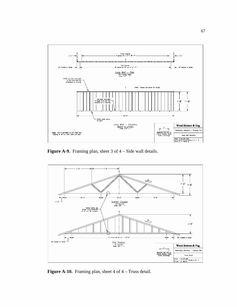
67

Figure A-9. Framing plan, sheet 3 of 4 – Side wall details.

Figure A-10. Framing plan, sheet 4 of 4 – Truss detail.

68

APPENDIX B

MODELING TECHNIQUES DESIGN ANALOG To make a computer model of any building, the real structure must be

idealized. This theoretical representation of the actual building geometry is called

the design analog. Studs, trusses, and other framing members are symbolized

simply as line segments in SAP2000, and a variety of design analogs are possible.

In this study, the line segments representing the wall framing members are

drawn through the centerlines of the actual building geometry. On the other hand,

the roof system (i.e. truss analog) does not use the centerlines, and instead follows

standard industry convention (Callahan 1993) – see Figure B-1. With this in mind,

as well as considering automatic meshing options, the actual footprint dimensions

of the SAP2000 structure are 29-ft 4-in wide by 40-ft long.

Figure B-1. Analog used in SAP2000.

69

SHELL ELEMENT BEHAVIOR

As noted in the SAP reference manual (Computers and Structures 2008),

the shell element is a type of area object that is used to model (1) membrane, (2)

plate, and (3) shell behavior. Membrane behavior only includes in-plane forces (no

out-of-plane). Plate behavior is the opposite – out-of-plane bending and transverse

shear are included but in-plane forces are not. The shell behavior is a combination

of the two. Thus, all forces and moments are supported. Further, two options exist

once the shell element is selected: thick or thin, both of which affect the out-of-

plane bending behavior. The thin shell neglects the effects of transverse shearing

deformation, while the thick shell includes them. To fully capture the behavior of

the roof and wall sheathing, the thick shell element, with full shell behavior, was

selected for use in this study.

Because each wall and roof area was defined using one shell element, it is

assumed that the actual 4-ft x 8-ft sheathing panels transfer load and moment

continuously across their joints. To explore this assumption, the wall and roof

systems are examined in greater detail. In a wall system, the panels are typically

placed vertically; therefore all edges of the panel are blocked (see Figure B-2).

Also, the nails are located within 3/8-inch of the panel edges, providing fixity

directly up to the joint line. In addition, nail spacing is at most 6-inches on center

along the edges. This continuous support system and high nail density give

credibility to the assumption of continuity across the joints for wall sheathing.

70

Figure B-2. Typical wall detail. Blocking along all edges of each panel and high nailing density at edges contribute to the assumption of continuity across individual panel joints.

In the roof structure, however, blocking is rarely used in residential

structures. Nevertheless, the edges of the plywood that fall upon truss lines are

nailed every 6-inches at the most, oftentimes less (i.e. 3 or 4-inches on center), and

the joints in this direction are staggered so as not to create a continuous line. Along

the unblocked edges, field nailing requires each nail to be located within 3/8-inch

on either side of the edge, so there are two nails within a distance of approximately

1-inch at these edges (see Figure B-3).

71

Figure B-3. Typical roof sheathing detail. The assumption of continuity across the joints is drawn from four sources: (1) staggered joints along truss lines, (2) 6-inch or less edge nail spacing along truss lines, (3) unblocked edges have nails within 3/8-inch from edge, and (4) “H-clips” at intermediate locations.

In addition, “H-clips” are recommended between adjacent panels and are located

midway between each pair of trusses. In lieu of these clips, tongue-and-groove

edges are recommended, also encouraging continuity across the joints (APA 2007).

With these considerations in mind, it is plausible that the roof panels, like the wall

panels, behave less as individual sheets and more as one cohesive unit.

MESHING OF THE SHELL ELEMENT

The automatic meshing option feature was used exclusively in this study.

The shell elements were meshed using either the “maximum size” option or the

72

“general divide” tool from the “Assign automatic area mesh” menu. Figure B-4

shows the inputs that are required to mesh a shell element using the “maximum

size” option.

Figure B-4. Meshing of shell elements based on maximum size. This option was used for the walls (between the top and bottom plate) and for the roof.

When the mesh is defined in this manner, SAP add points along each edge

of the area object (shell element) at equally spaced intervals such that the distance

between the points does not exceed the specified length, thereby creating a grid or

“mesh” over the area. For example, the length has been set to 16-inches in Figure

B-4. Consequently, SAP will divide the wall area into 16-in x 16-in grids. The

mesh can be refined as desired. Smaller grid spacing will result in a finer mesh, but

73

this comes at the expense of longer processing time. In this study, walls were

meshed to match the stud spacing (16-inches), and roof sheathing was meshed to

match the truss spacing (24-inches). In a few load cases, it was necessary to divide

the roof sheathing into smaller grids (12-inch meshing) based on the manner in

which the applied loads were defined. This brings up an interesting point. To

ensure that the framing members interact properly with the shell elements, it is

important to use a mesh size that is a multiple of the frame spacing in the area of

interest (e.g. for 24-inch truss spacing, mesh the roof elements at 6, 12, or 24

inches). When odd lengths are present within the structure, such as around

openings or at the very end of a wall, a separate shell element with its own unique

meshing option can be created. Alternatively, different meshing options such as

the “general divide” tool, described in the following paragraph, could be explored

in these cases.

The wall sheathing in the gable ends above the top plate was meshed using

the “general divide” option (see Figure B-5). The meshing group in this case

consisted of the framing members in the gable wall.

74

Figure B-5. Meshing of shell elements based on points and lines in a specified meshing group. This “general divide” option was used for the gable walls in the region above the top plate.

CONNECTIVITY

The members within the truss are connected using a mixture of pinned and

rigid connections (see Figure B-6). This configuration was used successfully in the

research effort conducted by Gupta and Limkatanyoo (2008). It is worth noting

that the joint representing the heel of the truss is not coincident with the connection

to the top plate of the wall. Since the analog of the wall members is drawn through

the centerlines, these two joints are offset by a distance of 1.75 inches (i.e. half the

width of the nominal 2-in x 4-in top plate). Both of these connections are rigid.

See Figures B-6 and B-7. Vertical web members in the gable end trusses and

75

Figure B-6. Connectivity of the trusses – mixture of pinned and rigid joints.

Figure B-7. Detail of the truss heel showing the offset between heel joint and connection to the top plate (1.75-inches).

76

overhang framing members were considered to be pinned at each end.

All members in the walls are pinned, including stud-to-plate connections (at

both ends) as well as plate-to-plate connections at the corners of the building (see

Figure B-8). In this configuration, the wall framing provides no lateral stiffness

unless sheathing is present.

Figure B-8. All connections within the wall are considered to be pinned.

STIFFNESS OF HOLD-DOWNS AND ANCHOR BOLTS

Established practices in the design of wood structures (Breyer 2007) specify

that hold-down devices carry vertical loads (i.e. axial) but no lateral loads (i.e.

shear). A separate set of anchorage devices, called anchor bolts, carry all of the

shear forces as well as resist wind uplift loads. Therefore, each hold-down device

in this study is modeled as one grounded spring having a stiffness in the Z-direction

77

alone (i.e. axial) while the anchor bolts are modeled as three grounded springs –

providing a stiffness in each of the X, Y, and Z-directions. The X and Y-directions

correspond to shear forces parallel and perpendicular to the wall, respectively,

while the Z-direction corresponds to vertical forces (i.e. axial stiffness). See

Figure B-9.

Figure B-9. Orientation of axes for anchor bolts and hold-down devices.

The axial stiffness of the hold-down device is listed by the manufacturer

(Simpson Strong-Tie, 2008). The most common type of connector, the HDU2, was

selected. The published axial stiffness of this connector is 35,000 lb/in. This value

takes into account fastener slip, hold-down elongation, and bolt elongation. The

axial stiffness of the anchor bolts, on the other hand, was determined using research

data from a previous study. Seaders (2004) subjected partially anchored walls to

lateral loads. These walls contained no hold-down devices whatsoever, isolating

78

the behavior of the anchor bolts. Vertical deflection was measured at both the

tension (inboard) and the compression (outboard) side of the walls as lateral load

was applied (Figure B-10). When plotted against the applied load, this data

provided axial stiffness values for the anchor bolt assembly in both tension and

compression. As it turned out, the stiffness values in compression were similar to

those in tension (Figure B-11). Because these tests were conducted on a full-scale

wall assembly and not on the anchor bolts themselves, this stiffness not only takes

into account bolt elongation, but also wood crushing, washer deformation, and

other similar real-world effects that take place when a structure is loaded. Values

were averaged for five different walls, resulting in a vertical stiffness of 33,000

lb/in. For practical purposes this value was rounded up to match the value of the

hold-down stiffness, so that both the anchor bolts and the hold-downs have the

same axial stiffness of 35,000 lb/in.

The shear stiffness of the anchor bolts in the X and Y-direction was

determined using a procedure recommended by the NDS (AF&PA 2005). It

suggests using the load-slip modulus value for wood-to-wood connections. This

may seem counterintuitive considering the anchor bolts connect wood to concrete

(i.e. bottom plate to foundation); however, the NDS value for dowel-type fasteners

(e.g. anchor bolts) is governed by the MOE of the main member and the side

member. Relatively speaking, the MOE of concrete is much closer to wood than it

is to steel, the other available load-slip value. In fact, the MOE of steel is one order

of magnitude greater than the MOE of wood and concrete (see Table B-1).

79

Vertical Deflection vs. Applied LoadSeaders (2004)

0

500

1000

1500

2000

2500

3000

3500

4000

0 0.1 0.2 0.3 0.4 0.5

Vertical Deflection (in)

App

lied

Load

(lbs

)

InboardOutboard

Figure B-10. Inboard and outboard vertical deflection measurements for a typical

partially anchored wall. (Seaders 2004)

Vertical Deflection vs. Applied LoadSeaders (2004)

y = 31,538x

y = 33,113x

0

200

400

600

800

1000

1200

1400

1600

1800

2000

0.00 0.01 0.02 0.03 0.04 0.05 0.06 0.07 0.08

Vertical Deflection (in)

App

lied

Load

(lbs

)

InboardOutboard

Figure B-11. Stiffness in the vertical direction for a typical partially anchored

wall. Five walls in total were averaged. (Seaders 2004)

80

Table B-1. Comparison of MOE values for determining the load-slip modulus.

Material Modulus of Elasticity(106 psi) Source

Wood 1-2 Askeland 1994 Concrete 4 Lardner 1994

Steel 29 Lardner 1994

For this reason, the American Wood Council recommends “for fasteners into

concrete, wood-to-wood values are used as a reasonably conservative approach”

(AF&PA 2007). Accordingly, the shear stiffness for the anchor bolts was

calculated using the load-slip modulus equation given in the NDS code as follows:

5.1000,180 D⋅=γ (lb/in) NDS 10.3.6

“D” in this equation is the diameter of the anchor bolt (1/2-inch). Therefore, a

value of 65,000 lb/in was used for the shear stiffness of the anchor bolts in the X

and Y-directions. Table B-2 summarizes the spring stiffness values used in this

study.

Table B-2. Spring stiffness used to model the anchor bolts and hold-downs.

Item

X-direction

(shear) lb/in

Y-direction

(shear) lb/in

Z-direction

(axial) lb/in

Source

Hold-downs - - 35,000 Simpson Strong-Tie (2008)Anchor

bolts 65,000 65,000 35,000 NDS (AF&PA 2005) and Seaders (2004)

81

MATERIAL PROPERTIES

Frame Elements

Frame elements, which represent the wall and truss members, were modeled

using elastic, isotropic material properties. Two parameters are required to define

these materials: the modulus of elasticity (MOE) and Poisson’s ratio. The shear

modulus is computed as a function of these two values using the following

equation.

( )µ+=12EG

MOE values were assigned using the NDS code (AF&PA 2005). Poisson’s ratio

for Southern Pine (SYP) was calculated using the average of the radial and

tangential values of the four species that comprise the group. For the Spruce-Pine-

Fir (SPF) group, Poisson’s ratio was based on three of the eight species that make

up the group. Data was not readily available for the remaining five species (USDA

1999).

Table B-3. Elastic isotropic material properties used in the SAP model.

MOE (106 psi) Poisson’s Ratio Item Description

Value Source Value Source Wall

members SPF, stud

grade 1.2 0.40

Truss members

SYP, No.3 and stud 1.4

NDS (AF&PA

2005a) 0.36

Wood Handbook (USDA 1999)

82

Shell Elements

Wall and roof sheathing were modeled using SAP’s thick shell element.

Orthotropic, elastic material properties were then assigned. Nine constants (six of

them independent) are needed to describe the behavior of these materials: three

moduli of elasticity, three shear moduli, and three Poisson’s ratio. The SAP

reference manual states that E3, µ13, and µ23 are “condensed out of the material

matrix” (Computers and Structures, 2008). In other words, they are dependent

properties. Additionally, the values of G13 and G23, which are used to compute the

transverse shearing stiffness, were found to have a negligible effect on the behavior

of the model. Thus, the only values that are truly of importance are shown in bold

in Table B-4. These represent the strong-axis MOE (E1), weak-axis MOE (E2), in-

plane shear modulus (G12), and in-plane Poisson’s ratio (µ12). SAP however

requires input values for the remaining parameters, so all values must be provided

per Table B-4.

Table B-4. Elastic orthotropic material properties used in the SAP model.

Description MOE (105 psi)

Shear Modulus (105 psi)

Poisson’s Ratio4

Item Type E1 E2 E3 G12 G13 G23 µ12 µ13 µ23 Wall

sheathing1,2 7/16” OSB 7.4 2.3 2.3 1.2 1.2 1.2 0.08 0.08 0.08

Roof sheathing3

½” Plywood 19 2.9 2.9 1.5 1.5 1.5 0.08 0.08 0.08

1 MOE and shear modulus values from Doudak (2005) 2 Shear modulus values subject to the correlation procedure (Table 4) 3 MOE and shear modulus values from Wolfe and McCarthy (1989) and Kasal (1992) 4 Poisson’s ratio from Kasal (1992)

83

DISCUSSION OF ASSUMPTIONS

Although the assumptions used in the modeling process have been

introduced and explained, their individual effect on the behavior of the model needs

to be discussed. For example, the assumption that the peak of each truss behaves as

a pinned connection, while the heel behaves as a rigid one, leads to slightly more

deflection in the upper portion of the top chords compared to the lower portion.

Also, because the heel joint is fixed, the angle between the top chord and the

bottom chord remains fixed as the truss deflects and the members experience in-

plane rotation. Thus, the rotation of the lower portion of the top chord is coupled

with a similar rotation in the bottom chord in the vicinity of the heel joint. This

behavior is obviously different than what takes place at the peak where the joint is

pinned. Near the ridge, any rotation of the top chord on one side of the roof is

essentially isolated from the other side of the roof by the pinned connection.

In addition to the assumptions of connectivity, the correlation model for the

nailing schedule of the sheathing has limitations. The correlation procedure,

described in the “Results and Discussion” section and in Appendix E, was

developed for shear walls 8-feet in length by 8-fee in height. However, the walls of

the index building are much longer than this. An explanation of the error

introduced by extending the correlation to these longer walls is provided in

Appendix E, but for the present discussion it is sufficient to point out that the error

increases as the shear walls increase in length and as the edge nail spacing

decreases (Figure E-8).

84

As previously discussed in this section, individual 4-ft x 8-ft plywood/OSB

panels were not modeled, and continuity was assumed across their joints. If the

panel joints actually behave more like hinges, or something between a pinned or

rigid connection, the load sharing behavior of the sheathing would be affected.

Specifically, the panels would not distribute load as effectively across their joints,

isolating behavior at one end of the building from the other end. In the case of the

roof assembly, however, the load sharing characteristics of the model (along with

the assumption of continuity across the panel joints) were compared to published

data with good agreement (Appendices C and D).

Finally, it should be noted that the assumption of linearity in the model

implies that the material properties of the constitutive elements remain in the

“linear-elastic” realm. That is, any elongation, rotation, or other type of deflection

experienced by the model would theoretically be recovered when the load is

removed. Implicit in this assumption is the fact that the load levels are assumed to

be within the linear realm as well. In other words, if load levels induce stresses

greater than the known proportional limit of the materials, the assumption of

linearity is no longer valid and the response of the model loses accuracy.

Consequently, it is worth pointing out that the loads encountered in the present

research study were sufficiently within the design load range such that the

assumption of linearity is valid. Although perhaps a limitation in one sense, the

assumption of linearity is essential in maintaining practicality in the modeling

process.

85

APPENDIX C

VALIDATING THE MODEL

VALIDATION

Two-Dimensional Truss Model Behavior

The truss model used in this study is comprised of either rigid or pinned

connections (see Appendix B, Figure B-6). These assumptions about connectivity

were validated against previous literature and experimental results. Wolfe et al.

(1986) subjected forty-two full-size trusses to vertical loads acting over the top

chord. Some of the trusses were tested to design loads, while others were loaded to

failure. The study included two different roof pitches (3:12 and 6:12) and three

different MOE categories (low, medium, and high). Li (1996) used Wolfe’s

research to validate his own analytical truss model. In his ETABS model, Li made

use of spring elements to represent the metal-plate-connected joints at the heel and

at the tension splice of the bottom chord. All other connections were assumed to be

pinned. Thus, Li’s model incorporated semi-rigid behavior that has purposely been

eliminated in the present effort. Consequently, these two previously published

studies serve as an excellent opportunity to validate the current SAP model.

The 6:12 roof pitch was selected, and a load of 66 lb/ft was applied along

the sloped length of the top chord (acting vertically). This load represents the total

design load for the truss. Four trusses from each MOE category were used for

comparison, and MOE values of the individual members were assigned based on

the values provided by Wolfe et al. 1986. In order to directly compare to the

86

reported results, deflections were averaged at the five interior panel point locations

(i.e. where the web members intersect the chord members) – see Figure C-1.

Deflections were compared at load levels within the design load range to ensure

that the response behavior remained within the linear-elastic realm. Table C-1

shows the comparison between the full-scale testing performed by Wolfe et al.

(1986), the spring-element ETABS model developed by Li (1996), and the

simplified SAP model used in the present study.

Figure C-1. SAP model for the 2D verification.

87

Table C-1. 2D verification – deflection comparison for 6:12 slope trusses tested to their design load. Percent difference values are included, comparing the two analytical models (the present effort and Li’s previous research) to the physical testing performed by Wolfe.

Deflection (in) Truss No. Wolfe et al.

1986 Present SAP

model 1 Li, 1996 2

6L2 0.172 0.179 4% 0.179 4% 6L3 0.180 0.186 3% 0.186 3% 6L5 0.194 0.176 -9% 0.176 -9% 6L7 0.198 0.175 -12% 0.175 -12%

Average for Low MOE 0.186 0.179 -4% 0.179 -4%

6M1 0.123 0.118 -4% 0.121 -2% 6M2 0.136 0.127 -7% 0.129 -5% 6M4 0.121 0.126 4% 0.127 5% 6M7 0.117 0.132 13% 0.133 14%

Average for Medium MOE 0.124 0.126 1% 0.128 3%

6H1 0.107 0.094 -12% 0.099 -7% 6H2 0.107 0.097 -9% 0.101 -6% 6H6 0.086 0.101 17% 0.104 21% 6H7 0.107 0.102 -5% 0.104 -3%

Average for High MOE 0.102 0.099 -3% 0.102 0%

1 Percent difference values compare the current SAP model to Wolfe et al. 2 Percent difference values compare Li’s ETABS model to Wolfe et al.

As highlighted in Table C-1, there is – on average – no more than 4%

difference between the present SAP model and the full-scale test results, which is

the same level of accuracy that Li was able to achieve with his spring-element

model. In fact, there is only 3% difference between the present simplified SAP

model and the more complicated ETABS spring-element model developed by Li.

Therefore, the simplified assumption of connectivity based on rigid and pinned

88

connections is deemed adequate for use in this study. This conclusion concurs with

the findings of Limkatanyoo (2003), who used the same arrangement of

rigid/pinned connections in his research. He compared a similar two-dimensional

SAP model to an industry-accepted program called VIEW widely used by truss

designers. Limkatanyoo checked both deflections and stresses (using the combined

stress index, CSI) and concluded that the simplified design analog was in

agreement with the more complicated, semi-rigid models employed by the truss

industry (i.e. the results from VIEW).

Three-Dimensional Truss Assembly Behavior

Once the model’s two-dimensional behavior was validated, the next step

involved the verification of its 3D response. To do this, a nine-truss roof assembly

was modeled in SAP for comparison to a full-scale test conducted at the Forest

Products Laboratory (Wolfe and McCarthy 1989). In this experiment, researchers

represented a 16-foot section from the middle of a conventional gable style roof in

order to quantify the effects of load sharing within an assembly of trusses. The

trusses were built with members from one of three MOE categories, resulting in a

nine-truss assembly comprised of three trusses from each stiffness category – low,

medium, and high. The variable stiffness trusses were located randomly within the

assembly to accentuate the effect of load sharing, the hypothesis being that greater

load would be carried by the stiffer trusses regardless of location within the

assembly.

89

Load sharing was quantified using influence matrices for both reactions and

deflections. In the case of the reactions, a “load influence matrix” was defined as

the sum of the vertical reactions at each truss expressed as a fraction of the total

applied load. For deflections, a similar “deflection influence matrix” was defined

as the deflections observed at each truss expressed as a fraction of the total

deflection for all trusses. At each truss, deflections were measured at four different

locations along the top chord and then averaged. First, load was applied

consecutively to each individual truss. Next, load was applied to all trusses at once

(i.e. full assembly load). In both cases, the load per truss was 66 lb/ft, as in the 2D

verification. It’s worth noting, though, that the magnitude of the load has little

effect on either the load sharing or the deflection sharing results within the 3D

assembly. This rather significant finding was observed by the researchers at the

FPL, noting that the load influence matrix “changed little with load level

throughout the linear load range” and “normalized deflections also show little

variation from one load step to the next within the linear range” (Wolfe and

McCarthy 1989). In other words, the influence matrices for load and deflection are

unaffected by changes in the magnitude of the applied load until the assembly

begins to experience damage.

Li (1996) attempted to model this same nine-truss assembly in his research.

Instead of using the shell element, whose behavior was not fully understood at the

time, Li modeled the plywood sheathing using beam elements. These plywood

“beams” had the same thickness as the plywood sheathing and their widths were

90

assigned according to their tributary length along the top chord. He used three

beams per roof section (six beams in total). To account for the partial composite

action between the sheathing and the top chords, which tends to increase the

flexural stiffness of the assembly, Li increased the bending capacity of the top

chord members by increasing their moment of inertia. In the present study, partial

composite action is inherently built into the model by way of the shell element.

Likewise, the need for “sheathing beams” is eradicated for the same reason.

Comparison plots between the present SAP model, the physical testing (Wolfe and

McCarthy 1989), and the “sheathing beam” model (Li 1996) are given in

Appendix D.

Insofar as load sharing is concerned when individual trusses are loaded,

there is 14% difference (on average) at the loaded truss between the SAP model

and the physical testing results. Li was able to achieve 13% difference with his

sheathing beam model. However, the striking difference between the two models

is not at the loaded truss, but rather at the non-loaded trusses. SAP shows an

average of 8% difference at the non-loaded trusses when compared to the physical

testing, while Li’s model predicts 26% difference. In other words, when trusses are

loaded individually, the two models predict load sharing at the loaded truss with

the same accuracy, whereas the shell element model is able to capture the load

sharing at the remaining trusses with much more accuracy than the sheathing beam

model. This trend can be observed in Table C-2 as well as the plots provided in

Appendix D (Figures D-1 to D-9). Similarly, the deflection sharing values also

91

showed good agreement with the experimental results when each truss was loaded

individually. At the loaded truss, the deflection sharing displayed 7% difference.

Non-loaded trusses exhibited only 1% difference (see Table C-3 and Appendix D,

Figures D-10 to D-18). Li did not include a deflection check in his research,

therefore a comparison cannot be made to his work beyond that which is provided

in Table C-2.

Table C-2. 3D verification – Absolute percent differences in load sharing when each truss is loaded individually (compared to Wolfe et al. 1989).

Present SAP Model (Shell Element)

Li, 1996 (Sheathing Beams) Loaded

Truss At Loaded Truss

At Non-Loaded Trusses

At Loaded Truss

At Non-Loaded Trusses

1 8 1 14 39 2 28 9 5 29 3 5 7 10 30 4 9 7 22 12 5 20 5 10 12 6 19 5 18 31 7 2 9 12 13 8 28 7 12 23 9 4 24 11 50

Average 14 % 8 % 13 % 26 %

Table C-3. 3D verification – Average percent differences in deflection sharing when each truss is loaded individually (compared to Wolfe et al. 1989).

Present SAP Model (Shell Element)

At Loaded Truss At Non-Loaded Trusses -7 % +1 %

92

The SAP model was also compared to the experimental tests when the

entire assembly was loaded simultaneously. Again, the results showed good

agreement (see Table C-4 and plots in Appendix D, Figures D-19 and D-20).

Individual deviations were limited to 12% difference in load sharing and 9%

difference in deflection sharing when compared to Wolfe et al. (1989). Li did not

include the full assembly load scenario in his research, so no comparison is made to

his work here.

Table C-4. 3D verification –Percent differences in load and deflection sharing when all trusses are loaded simultaneously (compared to Wolfe et al. 1989).

Present SAP Model (Shell Element) Truss Number

Load Sharing Deflection Sharing 1 2 -9 2 8 1 3 -12 -3 4 -10 -1 5 1 2 6 11 1 7 -4 0 8 6 0 9 1 3

As a result of three-dimensional verifications (consisting of two different load

scenarios), the shell element behavior was deemed adequate to predict the load

sharing and partial composite action response of the sheathing.

93

Shear Wall Behavior

In this study, three main variables were addressed in the investigation of the

shear wall behavior: (1) anchorage devices, (2) frame and shell behavior, and (3)

the nailing schedule of the wall sheathing. The anchor bolt and hold-down stiffness

values were determined from previous testing and from manufacturer’s data,

respectively (Appendix B, Table B-2). Also, the connectivity of the individual wall

members was established early in the study – all vertical studs were to be pinned at

each end (see Appendix B, Figure B-8). Lastly, the material properties, meshing

principles, and general behavior of the shell element were investigated and

documented (see Appendix B, Figure B-4 and Table B-4). Thus, the main purpose

of the shear wall behavior validation process was to develop a correlation between

the in-plane stiffness of the wall system in SAP and the nail spacing at the edges of

the OSB sheathing. Appendix E provides a detailed description of the process by

which the correlation was developed. Once established, the correlated SAP model

of the shear wall was compared to the experimental findings of several different

shear wall studies (see Appendix E, Figures E-2 to E-7). It should be noted that the

correlation procedure is valid only for the OSB sheathing used in this study. If

plywood were used as the wall sheathing material, a separate correlation would be

required using the Ga values provided in SDPWS Table A.4.3A (AF&PA 2005b).

Influence Functions

Once the 2D and 3D validations were complete, the final step involved

creating a SAP model of the entire building. However, this model of the index

94

building needed to be validated itself before proceeding. To do perform this

validation, analytical influence functions due to uplift were created using SAP and

were compared to experimentally determined results developed by researchers at

the University of Florida (Datin 2009). Appendix F provides a detailed description

of this investigation. Also presented in Appendix F is a comparison of results at

four selected locations within the structure (see Figures F-8 and F-9).

The result of this effort showed that the SAP model behaved in agreement

with the scaled physical testing. In general, influence functions of roof-to-wall

connections show that loads applied more than two trusses away from a point of

interest have very little effect at that point (Figure F-9, Load cells 2 and 15).

Within a distance of two trusses (48 inches), the effect of the load is greater. This

finding concurs with the results obtained from truss assembly tests performed at the

FPL (Wolfe and McCarthy, 1989). On the other hand, foundation connections

showed much less sensitivity to the location of the applied load (see Figure F-9,

Load cells 6 and 10). This occurs because the walls of the structure share the load

among all anchorage devices, effectively dissipating roof-level load intensities as

they make their way to the foundation (see Figure 6, 2-inch nailing). This type of

load sharing behavior is indicative of a stiff wall system (i.e. tighter nailing

schedule at the edges of the wall sheathing). As noted in the “Results and

Discussion” section of this report, the nailing schedule strongly influences the

ability of the walls to share roof-level loads. As edge nailing density is reduced

(i.e. nails are spaced farther apart), the walls become more flexible and are

95

therefore less capable of dissipating roof loads evenly at the foundation level – load

intensities become more prevalent (see Figure 6, 12-inch nailing).

The few discrepancies that exist between the experimental results and the

analytical ones can be attributed to a perceived difference in stiffness of the

respective structures. It is believed that the 1/3 scale prototype built at the

University of Florida is slightly more rigid than the SAP model due to the choice of

sheathing and fasteners that were employed. OSB in the prototype was ¼-inch

thick and sheathing nails were represented with ¾-inch long, #4 screws spaced at

four inches on center. The scaled OSB thickness was selected based on its out-of-

plane flexural stiffness under the presumption that this property would be of the

most interest for wind loads imparting uplift on the roof structure. Although this

notion holds true for the roof sheathing, it does not necessarily apply to the wall

sheathing, which is loaded in-plane in an uplift scenario. Further, the #4 screws

were selected to ensure that connection failure in uplift would not occur. The

researchers at the University of Florida found that the use of 1/3 scale nails led to

premature failure by way of nail withdrawal and sheathing pull-through. This

connection failure did not provide any insight into load paths or load sharing that

would otherwise be observable if the connections remained intact. Thus, the

decision was made to ensure that the connections between the sheathing and

framing did not fail, and the use of the #4 screws served this purpose (Datin 2009).

This choice of fastener, though, is assumed to contribute to the overall higher

rigidity of the structure, observable by the minor differences between the influence

96

function contour plots – especially at the foundation level (see Figure F-9, Load

cells 6 and 10).

97

APPENDIX D

3D VERIFICATION – LOAD SHARING STUDY The following plots provide a comparison between the present SAP model,

the physical testing (Wolfe and McCarthy 1989), and the “sheathing beam” model

(Li 1996). Appendix C provides a detailed description of this validation procedure.

LOAD SHARING WHEN TRUSSES ARE LOADED INDIVIDUALLY

Load distribution when TRUSS 1 is loaded (individually)

-20

-10

0

10

20

30

40

50

60

70

1 2 3 4 5 6 7 8 9

Truss Number

% L

oad

Dis

trib

utio

n

SAP2000 (shell element)

Li, 1996 (sheathing beam)

Wolfe et al.,1989

Figure D-1. Truss 1 loaded individually.

98


-10

0

10

20

30

40

50

60

1 2 3 4 5 6 7 8 9

Truss Number

% L

oad

Dis

trib

utio

n



Wolfe et al.,1989



-10

0

10

20

30

40

50

1 2 3 4 5 6 7 8 9

Truss Number

% L

oad

Dis

trib

utio

n



Wolfe et al.,1989


99


-10

0

10

20

30

40

50

1 2 3 4 5 6 7 8 9

Truss Number

% L

oad

Dis

trib

utio

n



Wolfe et al.,1989



-10

0

10

20

30

40

50

1 2 3 4 5 6 7 8 9

Truss Number

% L

oad

Dis

trib

utio

n



Wolfe et al.,1989


100


-10

0

10

20

30

40

50

1 2 3 4 5 6 7 8 9

Truss Number

% L

oad

Dis

trib

utio

n



Wolfe et al.,1989



-10

0

10

20

30

40

50

1 2 3 4 5 6 7 8 9

Truss Number

% L

oad

Dis

trib

utio

n



Wolfe et al.,1989


101


-10

0

10

20

30

40

50

60

1 2 3 4 5 6 7 8 9

Truss Number

% L

oad

Dis

trib

utio

n



Wolfe et al.,1989



-10

0

10

20

30

40

50

60

70

80

1 2 3 4 5 6 7 8 9

Truss Number

% L

oad

Dis

trib

utio

n



Wolfe et al.,1989


102

DEFLECTION SHARING WHEN TRUSSES ARE LOADED INDIVIDUALLY

Deflection sharing when TRUSS 1 is loaded (individually)

-10

0

10

20

30

40

50

60

70

1 2 3 4 5 6 7 8 9

Truss Number

Perc

enta

ge o

f ass

embl

y de

flect

ion


Wolfe et al., 1989


103


-10

0

10

20

30

40

50

1 2 3 4 5 6 7 8 9

Truss Number

Perc

enta

ge o

f ass

embl

y de

flect

ion


Wolfe et al., 1989



-10

0

10

20

30

40

50

1 2 3 4 5 6 7 8 9

Truss Number

Perc

enta

ge o

f ass

embl

y de

flect

ion


Wolfe et al., 1989


104


0

10

20

30

40

50

1 2 3 4 5 6 7 8 9

Truss Number

Perc

enta

ge o

f ass

embl

y de

flect

ion


Wolfe et al., 1989



0

10

20

30

40

50

1 2 3 4 5 6 7 8 9

Truss Number

Perc

enta

ge o

f ass

embl

y de

flect

ion


Wolfe et al., 1989


105


-10

0

10

20

30

40

50

1 2 3 4 5 6 7 8 9

Truss Number

Perc

enta

ge o

f ass

embl

y de

flect

ion


Wolfe et al., 1989



-10

0

10

20

30

40

50

1 2 3 4 5 6 7 8 9

Truss Number

Perc

enta

ge o

f ass

embl

y de

flect

ion


Wolfe et al., 1989


106


-10

0

10

20

30

40

50

60

1 2 3 4 5 6 7 8 9

Truss Number

Perc

enta

ge o

f ass

embl

y de

flect

ion


Wolfe et al., 1989



-10

0

10

20

30

40

50

60

70

1 2 3 4 5 6 7 8 9

Truss Number

Perc

enta

ge o

f ass

embl

y de

flect

ion


Wolfe et al., 1989


107

LOAD SHARING WHEN FULL ASSEMBLY IS LOADED

Load sharing when full assembly is loaded (simultaneously)

+1%

+6%

-4%

+11%

+1%

-10%

-12%

+8%

+2%

8

9

10

11

12

13

14

1 2 3 4 5 6 7 8 9

Truss Number

Perc

enta

ge o

f tot

al a

ssem

bly

load


Wolfe et al., 1989

Figure D-19. Load sharing when all trusses are loaded simultaneously.

108

DEFLECTION SHARING WHEN FULL ASSEMBLY IS LOADED

Load sharing when full assembly is loaded (simultaneously)

+3%

0%

0%

+1%

+2%-1%

-3%

+1%-9%

9

10

11

12

13

1 2 3 4 5 6 7 8 9

Truss Number

Perc

enta

ge o

f ass

embl

y de

flect

ion


Wolfe et al., 1989

Figure D-20. Deflection sharing when all trusses are loaded simultaneously.

109

APPENDIX E

CORRELATION TO NAILING SCHEDULE OF SHEATHING

The extent to which edge nailing affects diaphragm or shear wall stiffness is

dependent on the presence of blocking. Unblocked systems are relatively

unaffected by changes in the edge nailing. As previously noted residential, light-

frame roof systems fit into this unblocked category. On the other hand, wall

systems are blocked (assuming the typical practice of placing OSB panels

vertically). Therefore, this study focuses on the effect of edge nailing in the wall

sheathing.

For a given load value, the shear wall deflections predicted by the NDS

code were compared with those predicted by SAP (see Figure E-1). Code

deflections were computed using the SDPWS 3-term equation (AF&PA 2005b).

Generally, deflection in shear walls comes from four sources: bending of the

framing members, shear within the panel, nail slip between the panel and the

framing, and finally anchorage elongation. The SDPWS, a supplement to the NDS

code, however provides a simplified 3-term equation for computing shear wall

deflection. This 3-term equation combines the effects of panel shear and nail slip

into one term by way of a parameter called the apparent shear wall stiffness, Ga.

Also, the 3-term equation provides a linear relationship between load and

deflection, which is of particular interest in this study since the SAP model assumes

linear behavior as well. The SDPWS goes one step further and tabulates Ga values

for different nailing schedules, allowing the predicted deflection of a shear wall to

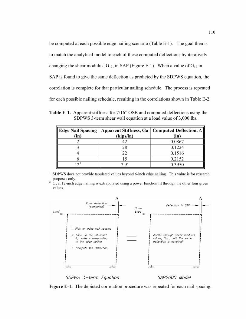
110

be computed at each possible edge nailing scenario (Table E-1). The goal then is

to match the analytical model to each of these computed deflections by iteratively

changing the shear modulus, G12, in SAP (Figure E-1). When a value of G12 in

SAP is found to give the same deflection as predicted by the SDPWS equation, the

correlation is complete for that particular nailing schedule. The process is repeated

for each possible nailing schedule, resulting in the correlations shown in Table E-2.

Table E-1. Apparent stiffness for 7/16” OSB and computed deflections using the SDPWS 3-term shear wall equation at a load value of 3,000 lbs.

Edge Nail Spacing (in)

Apparent Stiffness, Ga(kips/in)

Computed Deflection, ∆(in)

2 42 0.0867 3 28 0.1224 4 22 0.1516 6 15 0.2152

121 7.92 0.3950 1 SDPWS does not provide tabulated values beyond 6-inch edge nailing. This value is for research

purposes only. 2 Ga at 12-inch edge nailing is extrapolated using a power function fit through the other four given

values.

Figure E-1. The depicted correlation procedure was repeated for each nail spacing.

∆ ∆

111

Table E-2. Correlation between nailing schedule and the shear modulus G12 of the shell element in SAP.

Required G12 in SAP (104 psi) for each Edge Nail Spacing (inches) Sheathing

Stud Spacing

(in)

MOE of Members (106 psi) 2-in 3-in 4-in 6-in 12-in

7/16” OSB 16 or 24 1.2 to 1.6 9.43 6.38 4.86 3.34 1.81

The correlation procedure eliminated the effects of anchorage by setting this

term to zero in the 3-term equation and similarly by fixing the hold-downs in the

SAP model. Consequently, the values given in Table E-2 are entirely independent

of the anchorage system used, ensuring universal applicability in practice. The

correlation did however include the effects of deflection from frame bending in

order to investigate the effect of MOE and stud spacing. As it were, these two

factors presented no appreciable difference in the results of the correlation, again

making the values in Table E-2 universally applied over the ranges shown.

The correlated SAP model was compared to previously published

experimental results. Sinha (2007) tested 16 shear walls. 11 of these walls,

referred to as “Type A,” were sheathed with OSB on one side and gypsum

wallboard (GWB) on the other. The remaining 5 walls, referred to as “Type B,”

were sheathed with OSB alone (i.e. on one side only). Stud spacing for both was

24-in o.c. Lebeda (2002) tested a total of 13 walls under both monotonic and

earthquake loading (i.e. CUREE protocol). Of these tests, three were directly

comparable to the present study – the three monotonic tests of the control wall.

The control wall in this case was constructed using standard practices with studs

112

spaced at 16-in o.c. Finally, Langlois (2002) tested 14 shear walls, also under both

monotonic and earthquake load scenarios. Again, three tests were directly

comparable to the validation of the correlation procedure used in this study – the

first three monotonic wall tests. These walls had studs spaced 16-in o.c. Hold-

downs and anchor bolts were similar for all walls. Also, all of these shear wall

tests employed 4-in edge nailing and 12-in field nailing on the OSB sheathing.

Thus, there are a total of 22 walls to which the correlated SAP model can be

compared (see plots that follow, Figures E-2 to E-7). It should be noted that the

inclusion of the “Type A” walls from Sinah (2007), which were sheathed with a

combination of OSB and GWB, did not drastically increase the combined average

stiffness (compare Figures E-6 and E-7).

As can be seen in the plots (Figures E-3, E-5 to E-7), the correlated SAP

model reasonably predicts the deflection of the shear walls for the load range

shown. This load range corresponds to one-third the ultimate capacity of the walls,

or the practical linear response realm of the walls. The Type B, OSB-only walls

tested by Sinha (2007) display less stiffness than those tested by Lebeda (2002) and

Langlois (2002). It is presumed that this difference is attributed to the stud spacing.

Sinha’s walls used framing members spaced at 24-inches on center, while Lebeda

and Langlois employed 16-inch spacing. Conversely, the deflections predicted by

the SAP model and by the SDPWS 3-term equation do not depend on stud spacing.

Therefore, it is desirable that the correlated SAP model fall within the range of the

16-in and 24-in spacing tests, which it does (Figure E-5 to E-7). Figure E-7 shows

113

the SAP model to be within 0.07 inches (~1/16-inch) of the combined average at

one-third the ultimate capacity, translating into an error of approximately 30%

difference. Although not perfect, it should be pointed out that shear wall behavior

in this load range is difficult to measure and predict due to minor variations in

workmanship such as uneven nail spacing, tightness of bolts, etc. (Doudak 2005).

Thus, the resulting correlation method was deemed appropriate for use in this

study.

The range of applicability of the resulting correlation should be mentioned.

That is, the correlation procedure was performed considering shear walls with a

length and height of 8-feet by 8-feet in order to directly compare to published data

(Sinha 2007, Lebeda 2002, Langlois 2002). However, the walls in the index

building are significantly longer than this, i.e. 30-feet end walls and 40-feet side

walls. Since shear wall test data for walls of this length was not readily available,

the range of applicability was determined by comparing the predicted deflection

using the SDPWS 3-term equation against the deflection output of SAP. Thus, for

all walls of the index building, the shear wall deflection was computed at each

nailing schedule using the SDPWS method. Then similar length shear walls were

modeled in SAP and the deflection at all nailing schedules was determined using

the correlated G12 values provided in Table E-2. The error observed between the

two methods, in terms of predicted deflection, was then plotted as a function of

shear wall length (Figure E-8).

114

The two methods predict the same deflection for the 8-foot length walls

since this represents the original correlation. However, it can be seen that the

correlated G12 values (Table E-2) begin to over predict deflection both as the shear

wall length increases and as the edge nail spacing decreases. For the 6-inch edge

nail spacing used predominantly throughout this research effort, the error

introduced (in terms of predicted deflection) in the 30-ft end walls of the index

building is 5%, while 7% is shown in the 40-ft side walls (Figure E-8). To see the

effect that this error has on the correlated G12 value, the correlation procedure was

repeated using the 6-inch edge nailing for both the 30-ft end wall and the 40-ft side

wall. The result of this investigation showed that the 30-ft end wall would require

a G12 value of 3.51x104 psi, compared to 3.34x104 psi determined from the original

correlation. The percent difference between these two values is 5%, the same error

predicted by the deflection comparisons. In the case of the 40-ft side wall, the

required G12 value in order to match the predicted SDPWS deflection value is

3.58x104 psi. This value represents a 7% increase over the original correlated

value, again in line with what the deflection comparison revealed. In retrospect, it

is expected that the two comparisons (deflection and stiffness) should be tied to one

another, as they are. This results from the fact that the SAP model is linear,

meaning the assembly deflection is inversely proportional to the assembly stiffness.

In other words, if it is desired to decrease the deflection by 5%, the stiffness must

be increased by a similar amount.

115

Shear walls with OSB sheathingEdge nailing at 4-in o.c.

0.0

0.5

1.0

1.5

2.0

2.5

3.0

0.00 0.05 0.10 0.15 0.20 0.25 0.30 0.35 0.40 0.45

Deflection (in)

App

lied

Load

(kip

s)

Sinha (2007), Type B - 5 walls

Lebeda (2002) - 3 walls

Langlois (2002) - 3 walls

Figure E-2. OSB-only shear wall tests – 11 total walls.

Comparison to correlated SAP modelEdge nailing at 4-in o.c.

0.0

0.5

1.0

1.5

2.0

2.5

3.0

0.00 0.05 0.10 0.15 0.20 0.25 0.30 0.35 0.40 0.45

Deflection (in)

App

lied

Load

(kip

s)

Correlated SAP model at 4-in edge nailing




Figure E-3. Comparison to correlated SAP model at 4-in o.c. edge nailing.

116

Average stiffness of wallsEdge nailing at 4-in o.c.

0.0

0.5

1.0

1.5

2.0

2.5

3.0

0.00 0.05 0.10 0.15 0.20 0.25 0.30 0.35 0.40 0.45

Deflection (in)

App

lied

Load

(kip

s)




Figure E-4. Average stiffness for each type of wall study.

Comparison to correlated SAP modelEdge nailing at 4-in o.c.

0.0

0.5

1.0

1.5

2.0

2.5

3.0

0.00 0.05 0.10 0.15 0.20 0.25 0.30 0.35 0.40 0.45

Deflection (in)

App

lied

Load

(kip

s)





Figure E-5. Comparison of the correlated SAP model to the individual averages.

117

Combined average of all OSB walls (11 total)Edge nailing at 4-in o.c.

0.0

0.5

1.0

1.5

2.0

2.5

3.0

0.00 0.05 0.10 0.15 0.20 0.25 0.30 0.35 0.40 0.45

Deflection (in)

App

lied

Load

(kip

s)


Combined average - 11 walls




Figure E-6. Combined average of the OSB-only walls compared to the correlated

SAP model.

Combined average of ALL walls (22 total)Edge nailing at 4-in o.c.

0.0

0.5

1.0

1.5

2.0

2.5

3.0

0.00 0.05 0.10 0.15 0.20 0.25 0.30 0.35 0.40 0.45

Deflection (in)

App

lied

Load

(kip

s)


Combined average - 22 walls

Sinha (2007), Type A - 11 walls




Figure E-7. Include the OSB+GWB walls for a total comparison (22 walls).

118

% Error in Predicted Deflection As Length of Shear Wall Increases

-5

0

5

10

15

20

25

5 10 15 20 25 30 35 40

Length of Shear Wall (ft)

% E

rror i

n de

flect

ion

pred

ictio

n

2" edge nailing3" edge nailing4" edge nailing6" edge nailing12" edge nailing

SAP - SDPWSSDPWS

x 100%

Figure E-8. Percent error in predicted deflection as the length of the shear wall

increases.

119

APPENDIX F

INFLUENCE FUNCTIONS – CONTOUR PLOTS

Researchers at the University of Florida built a 1/3 scale model of the index

building (Figures F-1 to F-5) according to the framing plan shown in Appendix A

(Figures A-7 to A-10). The scale model followed proper structural scaling laws

and incorporated every last construction detail, including scaled metal plate

connectors designed by Gupta et al. (2005). Datin (2009) determined influence

functions for twenty load cells: 11 roof-to-wall and 9 wall-to-foundation (Figure F-

8). Of these twenty, four were selected for comparison – two roof-to-wall and two

foundation connections. The locations for comparison are highlighted in red in

Figure F-8. Uplift loads were applied to a dense grid on the roof using a pneumatic

actuator (Figure F-6). This grid is represented by the green dots in Figure F-7.

Hence, at each location corresponding to a green dot in Figure F-7, the pneumatic

actuator lifted up on the roof, and the reactions at all twenty load cells were

recorded. Loads were oriented normal to the roof plane and were applied in a step-

wise fashion, increasing from 10 lbs to 50 lbs at 10-lb increments. Similar to the

conclusion drawn by researchers at the FPL with their nine-truss roof assembly

(Wolfe et al., 1989), Datin also noted that load magnitude did not affect the

influence function results. Therefore the comparison to the SAP model used only

the highest load level of 50 lbs. Influence functions were determined by dividing

the measured reaction at the point of interest by the magnitude of the load applied

to the structure. This “influence value” was mapped to the location of the applied

120

load. For example, if the influence function for load cell no. 10 is desired, load

would be applied to the first green dot shown in Figure F-7 and the corresponding

reaction at load cell no. 10 would be recorded. This reaction would then be divided

by the magnitude of the applied load and mapped to the location on the roof where

the load was applied (i.e. the green dot). The process is repeated for all green dots,

and the resulting contour plot represents the influence function for load cell no. 10.

The entire procedure is repeated for all load cells.

Using SAP, a similar process was employed to develop the influence

function contour plots for the index building, with a couple of exceptions. First, the

load was scaled by a factor of nine (or the square of the length scale) to bring the

magnitude of the applied load from a 1/3 scale level to the full-scale level of the

SAP model. Thus, the uplift load magnitude was 450 lbs applied normal to the roof

surface. In SAP, this force was resolved into its vector components in the

horizontal and vertical direction since point loads are not readily applied normal to

a sloping surface in SAP. Second, the dense grid that Datin (2009) used (Figure

F-7) was modified slightly in SAP for simplification. Instead, a grid was assigned

based on 24-inch spacing. Load was iteratively applied, reactions were tabulated,

and comparable contour plots were generated (see Figure F-9). A discussion of the

results is provided in Appendix C.

121

Figure F-1. Construction of the 1/3 scale model at the University of Florida (Datin, 2009).


122


Figure F-4. Construction of the 1/3 scale model at the University of Florida (Datin, 2009). Location of load cells is highlighted.

123

Figure F-5. The completed 1/3 scale model at the University of Florida (Datin, 2009).

Figure F-6. The pneumatic actuator applied uplift loads normal to the roof.

124

Figure F-7. Uplift loads were applied consecutively at each green dot using a

pneumatic actuator.

1

789101112

1314

1617

1819

20

2

6

345151

789101112

1314

1617

1819

20

2

6

34515

Figure F-8. Load cell placement in the 1/3 scale wood frame house. Locations of comparison are highlighted in red.

125

Load Cell 2 Load Cell 6 Load Cell 10 Load Cell 15

(a) Experimental Influence Functions (1/3 scale model tests)

Load Cell 2 Load Cell 6 Load Cell 10 Load Cell 15

(b) Analytical Influence Functions (SAP 2000)

-0.2 0 0.2 0.4 0.6 0.8 1 1.2

Figure F-9. Comparison between influence functions determined

(a) experimentally and (b) analytically using SAP.

126

APPENDIX G

UNIFORM UPLIFT PRESSURE LOAD CASES

UNIFORM UPLIFT PRESSURE

With the validation steps complete, the index building was loaded in SAP

with a uniform pressure to study the general behavior of the structure over a range

of different geometry layouts. The uplift pressure was 50 psf applied normal to the

surface of the roof. Output plots (Figures G-1 to G-15) and deflected shapes

(Figures G-16 to G-24) are provided in the following figures. Deflections are

reported in inches. See the “Results and Discussion” section within the main body

of the thesis for further discussion.

127

Uniform pressure – Standard building 30’ x 40’


1200

1250

1300

1350

1400

1450

1500

1550

1600

1650

1700

4 52 58 64 70 76 82 88 5


Reac

tion

(lbs)




1600

1800

2000

2200

2400

2600

2800

3000

5 142 148 154 160 166 172 178 184 190 92


Reac

tion

(lbs)



Figure G-1. Uniform pressure, standard building geometry.


Uplift pressure = 50 psf (uniform)


128

Uniform pressure – Effect of nailing schedule


1100

1200

1300

1400

1500

1600

1700

1800

4 52 58 64 70 76 82 88 5

Joint ID

Reac

tion

(lbs)

2"3"4"6"12"

Gable walls Uniform pressure = 50 psf upliftNo ceiling


1500

1700

1900

2100

2300

2500

2700

2900

5 142 148 154 160 166 172 178 184 190 92

Joint ID

Reac

tion

(lbs)

2"3"4"6"12"

Eave walls Uniform pressure = 50 psf upliftNo ceiling

Figure G-2. Uniform pressure, standard building – effect of nailing schedule.




129

Uniform pressure – Extended building 30’ x 92’


1200

1250

1300

1350

1400

1450

1500

1550

1600

1650

1700

4 52 58 64 70 76 82 88 5


Reac

tion

(lbs)




1500

1700

1900

2100

2300

2500

2700

2900

3100

3300

3500

5 142 148 154 160 166 172 178 184 190 286 294 333 340 346 352 358 364 370 376 382 388 394 92


Reac

tion

(lbs)



Figure G-3. Uniform pressure, extended building.




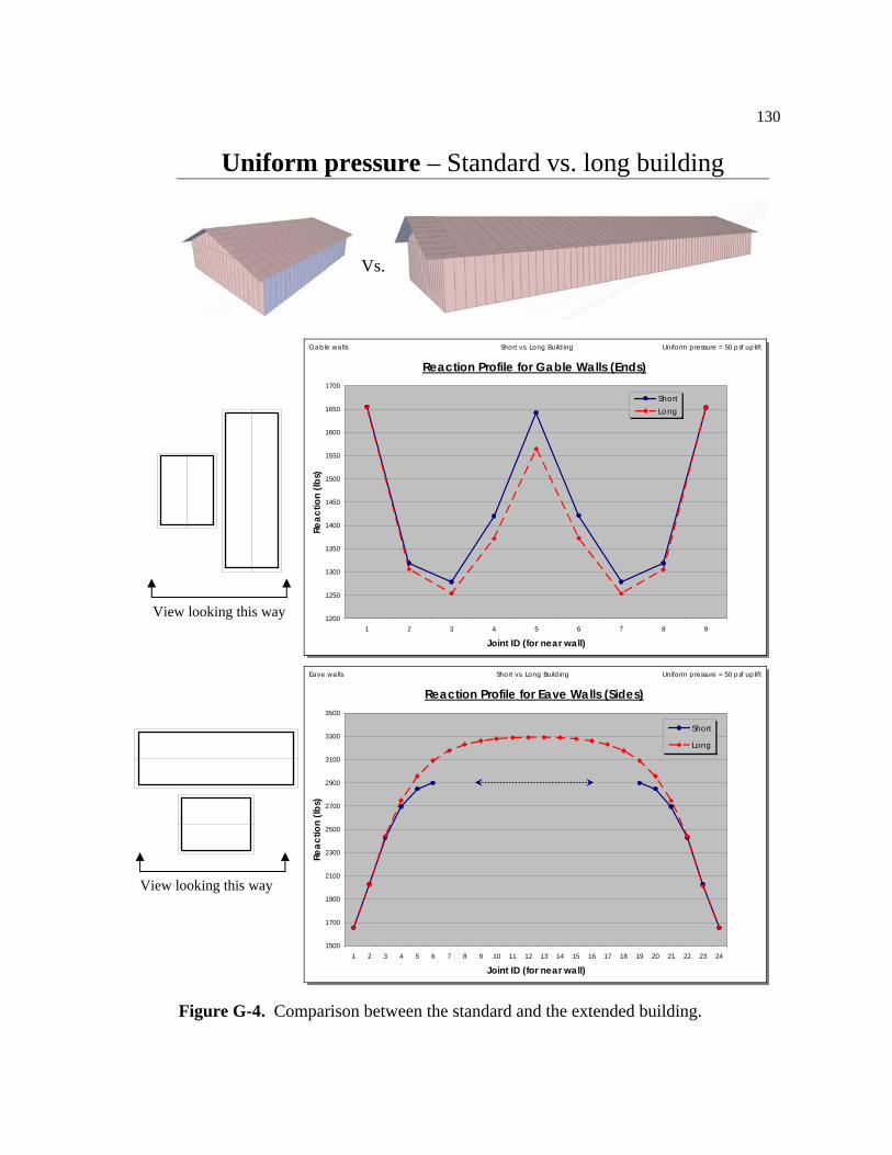
130

Uniform pressure – Standard vs. long building


1200

1250

1300

1350

1400

1450

1500

1550

1600

1650

1700

1 2 3 4 5 6 7 8 9


Reac

tion

(lbs)

ShortLong

Gable walls Uniform pressure = 50 psf upliftShort vs. Long Building


1500

1700

1900

2100

2300

2500

2700

2900

3100

3300

3500

1 2 3 4 5 6 7 8 9 10 11 12 13 14 15 16 17 18 19 20 21 22 23 24


Reac

tion

(lbs)

Short

Long

Eave walls Uniform pressure = 50 psf upliftShort vs. Long Building

Figure G-4. Comparison between the standard and the extended building.


Vs.


131

Uniform pressure – Door in gable wall (end wall)


0

500

1000

1500

2000

2500

4 52 58 64 70 76 82 88 5


Reac

tion

(lbs)

Near (with door)

Far (no door)




1500

1700

1900

2100

2300

2500

2700

2900

3100

5 142 148 154 160 166 172 178 184 190 92


Reac

tion

(lbs)




Figure G-5. Uniform pressure, door in end wall.




Far

Near

132

Uniform pressure – Door in side wall (centered)


1200

1300

1400

1500

1600

1700

1800

1900

4 52 58 64 70 76 82 88 5


Reac

tion

(lbs)

End walls (symmetric)Building without doors



0

500

1000

1500

2000

2500

3000

3500

4000

4500

5000

5 142 148 154 160 166 172 178 184 190 92


Reac

tion

(lbs)



Figure G-6. Uniform pressure, door in side wall.




Far

Near

133

Uniform pressure – Door in side wall (centered)

Reaction Profile for the Front Side Wall

1500

2000

2500

3000

3500

4000

4500

5000

5500

5 142 148 154 160 166 172 178 184 190 92

Joint ID

Reac

tion

(lbs)

12" header

24" header

With GWB ceiling

Building without door

Eave wall - with door Uniform pressure = 50 psf uplift

Reaction Profile for the Back Side Wall

1500

1700

1900

2100

2300

2500

2700

2900

3100

4 200 206 212 218 224 230 236 242 248 95

Joint ID

Reac

tion

(lbs)

12" header24" headerWith GWB ceilingBuilding without doors

Eave wall - back side (no door) Uniform pressure = 50 psf uplift

Figure G-7. Uniform pressure, door in side wall – effect of header depth and ceiling.


Effect of header depth and the presence of a gypsum wallboard (GWB) ceiling.


134

Uniform pressure – Door in side wall (not centered)


1200

1300

1400

1500

1600

1700

1800

1900

2000

2100

2200

4 52 58 64 70 76 82 88 5


Reac

tion

(lbs)




0

1000

2000

3000

4000

5000

6000

5 142 148 154 160 166 172 178 184 190 92


Reac

tion

(lbs)



Figure G-8. Uniform pressure, door in side wall – not centered.




Far

Near

Far

Near

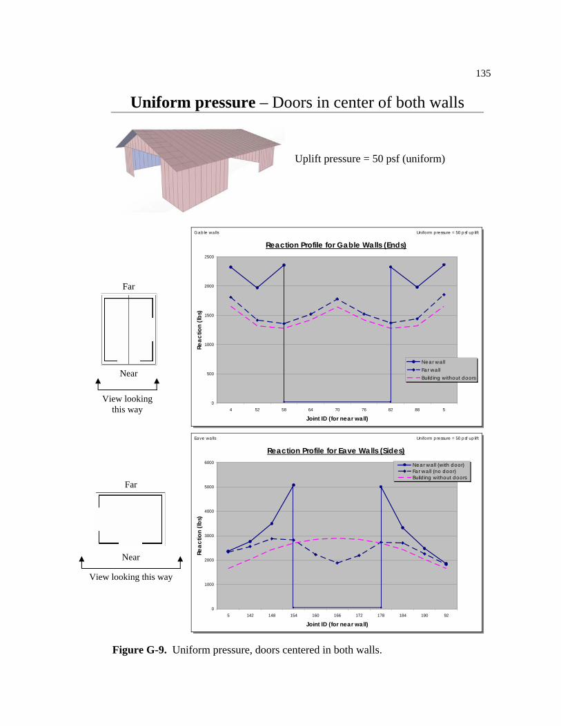
135

Uniform pressure – Doors in center of both walls


0

500

1000

1500

2000

2500

4 52 58 64 70 76 82 88 5


Reac

tion

(lbs)




0

1000

2000

3000

4000

5000

6000

5 142 148 154 160 166 172 178 184 190 92


Reac

tion

(lbs)



Figure G-9. Uniform pressure, doors centered in both walls.




Far

Near

Far

Near

136

Uniform pressure – Gable wall missing

Reaction Profile for Gable Wall (Back)

1000

1100

1200

1300

1400

1500

1600

1700

1800

4 52 58 64 70 76 82 88 5


Reac

tion

(lbs)

Far wall




1000

1500

2000

2500

3000

3500

4000

4500

5000

5 142 148 154 160 166 172 178 184 190 92


Reac

tion

(lbs)




Figure G-10. Uniform pressure, gable wall missing.




Far

Near

137

Uniform pressure – Blocked vs. Unblocked


1200

1250

1300

1350

1400

1450

1500

1550

1600

1650

1700

4 52 58 64 70 76 82 88 5

Joint ID

Reac

tion

(lbs)

UnblockedBlocked



1500

1700

1900

2100

2300

2500

2700

2900

3100

5 142 148 154 160 166 172 178 184 190 92

Joint ID

Reac

tion

(lbs)

UnblockedBlocked


Figure G-11. Uniform pressure, blocked vs. unblocked roof assembly.


Uplift pressure 50 psf (uniform)


Vs.

138

Uniform pressure – Outlooker vs. Ladder Overhang


1200

1250

1300

1350

1400

1450

1500

1550

1600

1650

1700

4 52 58 64 70 76 82 88 5

Joint ID

Reac

tion

(lbs)

OutlookerLadder



1500

1700

1900

2100

2300

2500

2700

2900

3100

5 142 148 154 160 166 172 178 184 190 92

Joint ID

Reac

tion

(lbs)

OutlookerLadder


Figure G-12. Uniform pressure, effect of changing the overhang framing style.



Outlooker-style Ladder-style

Vs.

139

Uniform pressure – Effect of anchor bolt spacing


1200

1400

1600

1800

2000

2200

2400

2600

0 5 10 15 20 25 30

Distance along wall (ft)

Reac

tion

(lbs)

4-ft spacing6-ft spacing



1500

2000

2500

3000

3500

4000

4500

5000

0 5 10 15 20 25 30 35 40


Reac

tion

(lbs)

4-ft spacing6-ft spacing


Figure G-13. Uniform pressure, effect of anchor bolt spacing (4-ft vs. 6-ft).




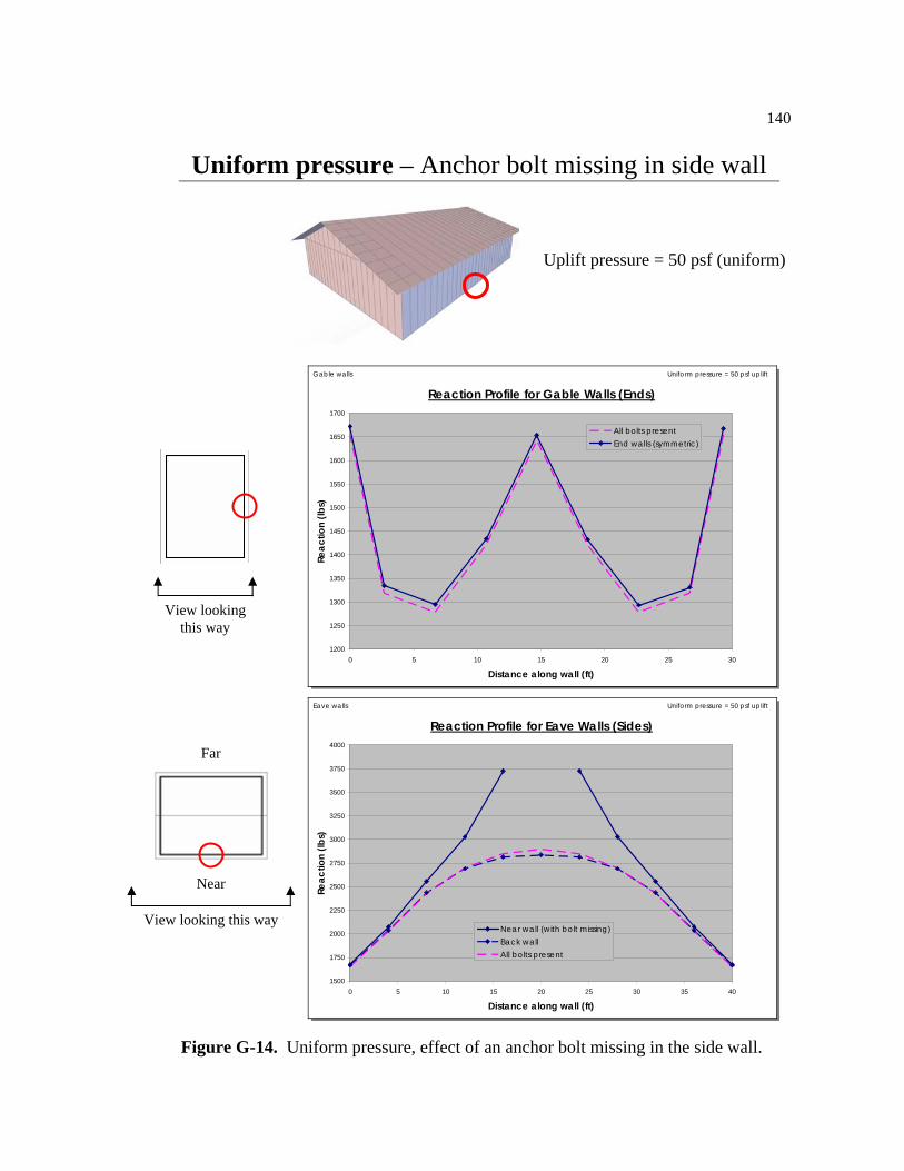
140

Uniform pressure – Anchor bolt missing in side wall


1200

1250

1300

1350

1400

1450

1500

1550

1600

1650

1700

0 5 10 15 20 25 30


Reac

tion

(lbs)

All bolts presentEnd walls (symmetric)



1500

1750

2000

2250

2500

2750

3000

3250

3500

3750

4000

0 5 10 15 20 25 30 35 40


Reac

tion

(lbs)

Near wall (with bolt missing)Back wallAll bolts present


Figure G-14. Uniform pressure, effect of an anchor bolt missing in the side wall.




Near

Far

141

Uniform pressure – Anchor bolt missing in gable wall


1200

1300

1400

1500

1600

1700

1800

1900

0 5 10 15 20 25 30


Reac

tion

(lbs)

Near (with bolt missing)Far wallAll bolts present



1500

1700

1900

2100

2300

2500

2700

2900

3100

0 5 10 15 20 25 30 35 40


Reac

tion

(lbs)

Side walls (symmetric)All bolts present


Figure G-15. Uniform pressure, effect of an anchor bolt missing in the gable wall.




Near

Far

142

Figure G-16. Deflected shape – standard geometry (control case). Deflections reported in 10-3 inches.

Figure G-17. Deflected shape – extended building. Deflections reported in 10-3 inches.

143

Figure G-18. Deflected shape – door in gable wall. Deflections reported in 10-3 inches.

Figure G-19. Deflected shape – door in side wall (centered). Deflections reported in inches.

144

Figure G-20. Deflected shape – door in side wall (not centered). Deflections reported in inches.

Figure G-21. Deflected shape – doors centered in both walls. Deflections reported in inches.

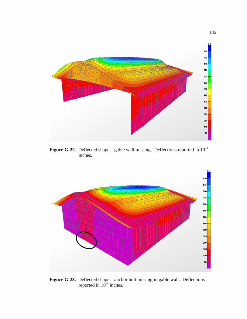
145

Figure G-22. Deflected shape – gable wall missing. Deflections reported in 10-3 inches.

Figure G-23. Deflected shape – anchor bolt missing in gable wall. Deflections reported in 10-3 inches.

146

Figure G-24. Deflected shape – anchor bolt missing in side wall. Deflections reported in 10-3 inches.

147

APPENDIX H

SIMULATED HURRICANE PRESSURES

BACKGROUND

Datin and Prevatt (2007) subjected a 1:50 scale model of the index building

(Figures H-1 and H-2) to simulated hurricane force winds, equivalent to a 3-second

gust wind speed of 130 mph. The tests were conducted in the atmospheric

boundary layer wind tunnel of the Wind Load Test Facility (WLTF, now called the

Wind and Structural Engineering Research Facility) at Clemson University. The

model was outfitted with 387 pressure taps installed on its roof, and the testing was

conducted at each of the five following wind directions: 0°, 45°, 90°, 135°, and

180°. Pressure was sampled at 300 Hz and recorded for 2 minutes, resulting in

36,000 pressure readings at each tap for each wind direction.

Figure H-1. Wind tunnel arrangement for 1:50 scale model of index building in suburban terrain. (Datin and Prevatt, 2007)

148

Figure H-2. 1:50 scale model of the index building (left). Dots indicate pressure taps (right). (Datin and Prevatt, 2007)

LOAD CASES

From these pressure time history files, three load cases were selected as

input cases for the SAP model in order to observe the response of the structure to

the simulated hurricane wind loads:

1. Absolute maximum uplift at the corner of the roof

2. Local maxima for all pressure taps

3. Absolute maximum uplift at the ridge of the roof

Load case 1 represents the time step associated with the maximum uplift

pressure experienced at the corner of the roof over all time steps for all wind

directions. Therefore, load case 1 signifies the instantaneous moment while the

absolute maximum uplift is occurring at the corner of the roof. Load case 2 is a

compilation of the local maxima for all pressure taps at the 45° wind direction,

regardless of where they occur in the history file. These maxima are combined and

149

applied to the roof structure simultaneously. Load case 3 is similar to case 1 except

the point of interest is at the ridge, not at the corner. Thus, load case 3 represents

the time step in the history files associated with the absolute maximum uplift

pressure observed at the ridge, which also happens to correspond to the 45° wind

direction.

MODELING

In order to input the pressures into SAP, a 2-ft by 2-ft grid was

superimposed over the actual roof pressure contours. For all three load cases, each

individual grid region was assigned the prevalent pressure within its perimeter.

Then the roof structure in the SAP model was divided in the same fashion and

loaded with the discrete pressures. In this way, the “analog” pressures provided by

the wind tunnel tests were “digitized” for input into the analytical model (see

Figures H-3 to H-5). The following plots represent the vertical foundation

reactions for each wall within the structure. The edge nailing of the wall sheathing

is 6-inches on center. Positive values represent uplift, for both applied pressure and

observed reactions. A discussion of the results is provided in the “Results and

Discussion” section of the main thesis. Figures H-6 to H-11 show the deflected

shapes for each load case. Deflections are reported in inches (positive values

represent uplift).

150

Load Case 1 – Maximum pressure at the corner


0

100

200

300

400

500

600

700

800

4 52 58 64 70 76 82 88 5


Reac

tion

(lbs)

WindwardLeeward

Gable walls Load case 1 - corner uplift


300

350

400

450

500

550

600

650

700

750

800

5 142 148 154 160 166 172 178 184 190 92


Reac

tion

(lbs)

Windward

Leeward

Eave walls Load case 1 - corner uplift

Figure H-3. Wind tunnel pressures, load case 1.



Wind direction

Leeward

Windward

Leeward

Windward


151

Load Case 2 – Local maxima over entire roof


0

200

400

600

800

1000

1200

1400

1600

1800

4 52 58 64 70 76 82 88 5


Reac

tion

(lbs)

Windward

Leeward

Gable walls Load case 2 - local maxima


0

200

400

600

800

1000

1200

1400

1600

1800

5 142 148 154 160 166 172 178 184 190 92


Reac

tion

(lbs)

WindwardLeeward

Eave walls Load case 2 - local maxima




Wind direction

Leeward

Windward

Leeward

Windward


152

Load Case 3 – Maximum pressure at ridge


200

300

400

500

600

700

800

900

4 52 58 64 70 76 82 88 5


Reac

tion

(lbs)

Windward

Leeward

Gable walls Load case 3 - max. pressure at ridge


200

300

400

500

600

700

800

900

1000

5 142 148 154 160 166 172 178 184 190 92


Reac

tion

(lbs)

Windward

Leeward

Eave walls Load case 3 - max. pressure at ridge




Wind direction

Leeward

Windward

Leeward

Windward


153

Figure H-6. Deflected shape – load case 1. Deflections reported in 10-3 inches.

Figure H-7. Deflected shape – load case 1 (view looking down). Deflections reported in 10-3 inches.

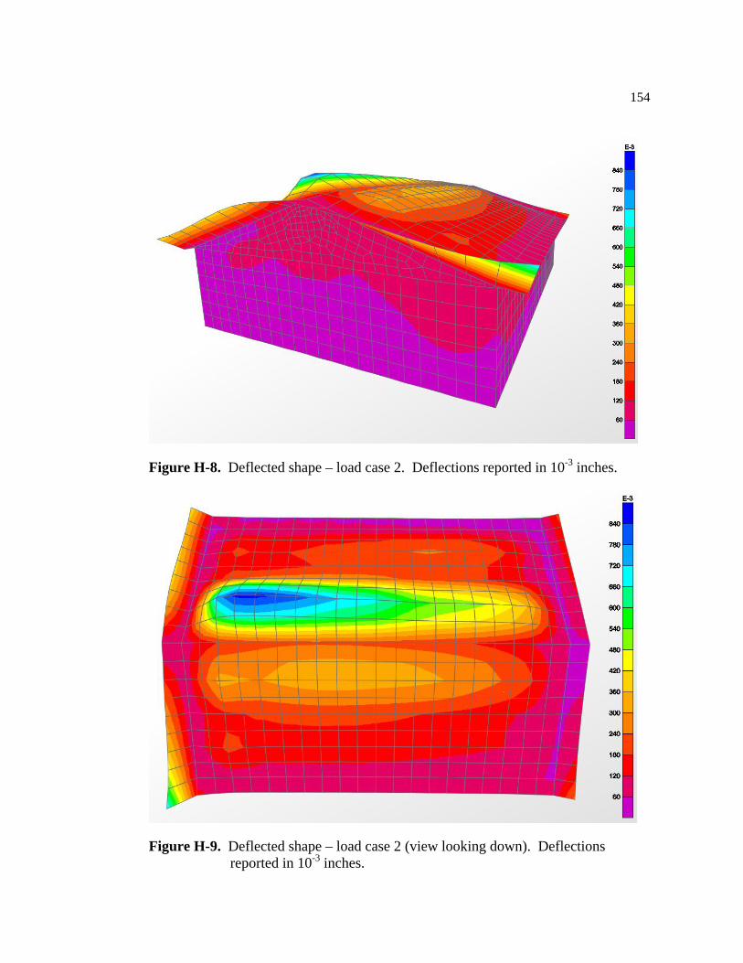
154


Figure H-9. Deflected shape – load case 2 (view looking down). Deflections reported in 10-3 inches.

155


Figure H-11. Deflected shape – load case 3 (view looking down). Deflections

reported in 10-3 inches.

156

APPENDIX I

ASCE 7-05 LOAD CASES

“C&C” vs. “MWFRS” PRESSURES

ASCE 7-05 provides separate provisions for wind design using loads for

either the “Main Wind Force-Resisting System” (MWFRS) or for “Component and

Cladding” (C&C) members. C&C loads were created by ASCE to represent peak

gusts which occur over small areas as a result of localized funneling and

turbulence. The localized loads can cause failures which in turn can affect the

overall “Main Wind Force-Resisting System” (MWFRS). Elements of the building

which are either “loaded directly by the wind or receive wind loads originating at

relatively close locations” are categorized as components and cladding (Douglas

and Weeks, 2003). On the other hand, members which make up the MWFRS are

considered to be assemblages of major structural elements that provide support and

stability for the overall structure. MWFRS members are generally not loaded

directly by the wind, but rather receive wind loads by way of the components and

cladding. Some elements can be identified in both systems (e.g. structural

sheathing), making the interpretation of the code intentions complicated. One

suggested interpretation is to design these components independently for each load

scenario, requiring two separate analyses. However, it has been noted that the

C&C load case attempts to address the “worst case” scenario (Douglas and Weeks,

2003). Also, roof sheathing uplift is a primary concern in major wind events, and it

is presumed that this failure results from localized effects acting on the roof

157

structure. Thus, for this project, component and cladding (C&C) pressures were

deemed the appropriate choice for determining the loads acting upon the index

building.

APPLIED LOADS

“Component and Cladding” (C&C) pressures were computed using the

analytical procedure (Method 2, ASCE 7-05). The simplified procedure (ASCE

Method 1) was employed as well, but the more comprehensive analytical approach

(ASCE Method 2) was selected to ensure accuracy and minimize generalizations.

After using both methods and comparing the results side by side, though, it should

be noted that the ASCE simplified procedure provides identical wind loads to the

analytical approach for the index building used in this study.

The structure was considered to be enclosed, and the maximum uplift

pressures were determined by considering the ASCE case of positive internal

pressure. For direct comparison to Datin and Prevatt’s research (2007), a basic

wind speed of 130 mph was used in the calculations. The following assumptions

and classifications were made in order to determine the appropriate wind loads for

the index building:

• Exposure category B [ASCE 7-05, 6.5.6.3]

• Topographic factor, Kzt = 1.0 [ASCE 7-05, 6.5.7]

• Occupancy category II [ASCE 7-05, Table 1-1]

• Importance factor, I = 1.0 [ASCE 7-05, Table 6-1]

158

Thus, ASCE 7-05 Figure 6-3 provides net design wind pressures at this basic wind

speed for the index building. These applied pressures are given in Table I-1. Roof

and overhang pressures represent uplift while wall pressures represent lateral loads.

The zones identified are shown in ASCE 7-05 Figure 6-3, and they are also

provided here in Figures I-1 and I-2.

Table I-1. Applied pressures using ASCE 7-05 for “Components and Cladding.”

Description Zone Pressure (psf)1 27.8 2 48.4 Roof 3 71.6

2A 56.7 Overhangs 3A 95.3 4 31.6 Walls 5 38.0

LOAD CASES

Three scenarios were considered with the ASCE 7-05 pressures: (1) uplift

acting alone, (2) lateral forces acting alone, and (3) a combination of both – lateral

in conjunction with uplift. Output plots as well as applied pressure values for the

three load cases are provided in the following plots – Figures I-1 to I-5. The

deflected shape for each scenario is shown in Figures I-6 to I-8. Deflections are

reported in inches.

159

ASCE 7-05 Pressures – Uplift loads acting alone


1200

1300

1400

1500

1600

1700

1800

4 52 58 64 70 76 82 88 5


Reac

tion

(lbs)


Gable walls ASCE 7-05 C&C pressures


1600

1700

1800

1900

2000

2100

2200

2300

5 142 148 154 160 166 172 178 184 190 92


Reac

tion

(lbs)


Eave walls ASCE 7-05 C&C pressures

Figure I-1. ASCE 7-05 pressures, uplift loads acting alone.



Pressures shown represent uplift applied normal to the roof plane

Zone 1 Interior 28 psf

Zone 2 Ends 48 psf

Zone 2A End overhangs 57 psf

Zone 3 Corners 72 psf

Zone 3A Corner overhangs 95 psf

160

ASCE 7-05 Pressures – Lateral loads acting alone


-1000

-800

-600

-400

-200

0

200

400

600

800

1000

4 52 58 64 70 76 82 88 5


Reac

tion

(lbs)

WindwardLeeward

Gable Walls ASCE 7-05 C&C pressures - (NO UPLIFT LOADS)


-1000

-800

-600

-400

-200

0

200

400

600

800

1000

5 142 148 154 160 166 172 178 184 190 92


Reac

tion

(lbs)

WindwardLeeward

Eave walls ASCE 7-05 C&C pressures - (NO UPLIFT LOADS)

Figure I-2. ASCE 7-05 pressures, lateral loads acting alone.


Zone 4 Interior 32 psf

Zone 5 Ends 38 psf

Pressures shown represent lateral loads applied normal to the wall plane


161

ASCE 7-05 Pressures – Lateral + Uplift


800

1000

1200

1400

1600

1800

2000

2200

2400

2600

4 52 58 64 70 76 82 88 5


Reac

tion

(lbs)

Windward

Leeward

Gable walls ASCE 7-05 C&C pressures -LATERAL + UPLIFT


800

1000

1200

1400

1600

1800

2000

2200

2400

2600

5 142 148 154 160 166 172 178 184 190 92


Reac

tion

(lbs)

WindwardLeeward

Eave walls ASCE 7-05 C&C pressures -LATERAL + UPLIFT

Figure I-3. ASCE 7-05 pressures, lateral plus uplift loads.



+Lateral Uplift

162

ASCE 7-05 vs. Wind Tunnel Tests

Reaction Profile for Gable Wall (Windward)

0

200

400

600

800

1000

1200

1400

1600

1800

2000

4 52 58 64 70 76 82 88 5

Joint ID

Reac

tion

(lbs)


Gable wall - Windward side All load cases

Reaction Profile for Gable Wall (Leeward)

0

200

400

600

800

1000

1200

1400

1600

1800

2000

95 98 104 110 116 122 128 134 92

Joint ID

Reac

tion

(lbs)


Gable wall - Leeward side All load cases

Figure I-4. ASCE 7-05 uplift response compared to the wind tunnel simulations.


Vs.


163

ASCE 7-05 vs. Wind Tunnel Tests

Reaction Profile for Eave Wall (Windward)

0

500

1000

1500

2000

2500

3000

1 2 3 4 5 6 7 8 9 10 11

Joint ID

Reac

tion

(lbs)


Eave wall - Windward side All load cases

Reaction Profile for Eave Wall (Leeward)

0

500

1000

1500

2000

2500

3000

4 200 206 212 218 224 230 236 242 248 95

Joint ID

Reac

tion

(lbs)


Eave wall - Leeward side All load cases

Figure I-5. ASCE 7-05 uplift response compared to the wind tunnel simulations.

Vs.



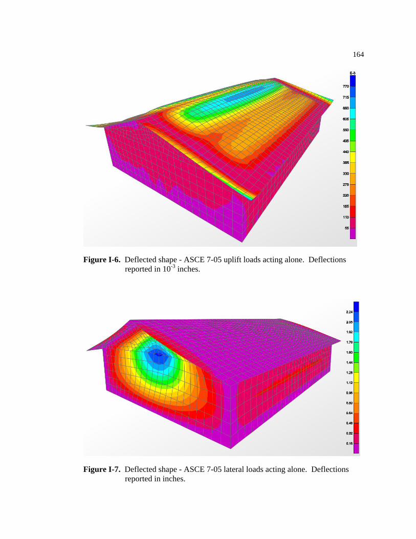
164

Figure I-6. Deflected shape - ASCE 7-05 uplift loads acting alone. Deflections reported in 10-3 inches.

Figure I-7. Deflected shape - ASCE 7-05 lateral loads acting alone. Deflections reported in inches.

165

Figure I-8. Deflected shape - ASCE 7-05 lateral + uplift loads. Deflections reported in inches.

166

APPENDIX J

ROOF SHEATHING UPLIFT CALCULATION

HAND CALCULATION

Assumptions

1. 8d common nails are used to secure the ½-inch thick roof sheathing panels.

a. This is required by the IBC as a minimum for wood structural panels.

b. This is also recommended by the APA – Roof Sheathing Fastening

Schedules for Wind Uplift (APA 2006).

2. The specific gravity of the framing members (i.e. truss top chords) is 0.49 or

greater.

a. This assumption is valid for common species such as Douglas-Fir-Larch

(North) and Southern Pine.

3. ASCE 7-05 “Component and Cladding” (C&C) pressures are used with a basic

wind speed of 130 mph, exposure B, and mean roof height less than 15-ft.

a. The maximum uplift pressure is 95 psf (see Appendix I, Table I-1 and

Figure I-1).

167

Computation

• Multiply the maximum applied C&C pressure by the tributary length of the roof

sheathing:

( )inlb

ftlbft

ftlb 8.151902952 ==⎟⎟⎠

⎞⎜⎜⎝

⎛

This represents the amount of force pulling up along the truss line (Figure

J-1).

• Divide this value by the allowable nail withdrawal value for wind design.

Allowable nail withdrawal value for wind design (CD = 1.6):

lbsW 97=′ [WFCM, Table 7A]

(See note on the following page regarding this value)

innails

naillbinlb

163.097

8.15=

⎟⎠⎞

⎜⎝⎛

⎟⎠⎞

⎜⎝⎛

• Invert this result to determine the number of inches per nail:

nailinches

innails 13.6

163.0

1=

• If the distance between nails is greater than this value, the uplift pressure will

exceed the capacity of the nail to prohibit withdrawal. Thus, the provided

field nailing must be 6-inches or less.

• For the conditions shown, 12-inch field nailing is not adequate to prevent

sheathing uplift.

(refer to Figure J-1)

168

Note: The allowable nail withdrawal value, W, can also be determined using the

following NDS procedure. The convenience of the WFCM becomes readily

apparent in comparing the number of steps that follow to the single tabulated value

provided by the WFCM.

8d common nail, D = 0.131” and L = 2.5” [NDS Table L4]

This translates into 2-inches of nail penetration with ½-inch roof sheathing.

Nail withdrawal, DGW 251380= [NDS Eq.(11.2-3)]

( )( ) ( ) 4.30131.049.01380 25 ==W lbs per inch of penetration

( ) lbsnpenetratioinchinlbsW 8.6024.30 =⎟

⎠⎞

⎜⎝⎛=

Adjusted withdrawal for wind design,

( ) 2.976.18.60 ==⎟⎠⎞

⎜⎝⎛=′ DC

naillbW lbs per nail

Compare this value to the one conveniently tabulated by the WFCM,

(Table 7A).

169

Figure J-1. Typical roof sheathing panel with 6-inch edge nailing and 12-inch field nailing. The magnitude of the force per lineal inch is only applicable for the applied pressure (95 psf) given in the example calculation.

170

ANALYTICAL PREDICTIONS – SHEATHING UPLIFT

SAP provides an output feature which allows the user to display “element

joint forces” for the shell element. The user can tabulate these forces for every

structural element used in the analytical model (frames, shells, etc.), essentially

providing a free-body-diagram for all the individual components. For example,

output is provided at the corners of meshed regions for the shell element.

Specifically, the roof shell element is subdivided into 2-ft by 2-ft squares, and joint

forces are provided at the joints representing corners of these squares. So the user

must pick a location of interest and manually combine the joint forces, considering

the contribution from each of the surrounding meshing regions. This process is not

only laborious, but also ineffective without further study. It is unclear at this time

how SAP allocates the internal forces between these components. Efforts to gain

insight into this topic were not readily understood using simplified models, so no

attempt was made to develop this undertaking further, given the complexity of the

model at hand. Further investigation is recommended.

171

APPENDIX K

LITERATURE REVIEW

ANALYTICAL MODELING

Joint Connectivity

When building an analytical model with a structural analysis program, the

designer is immediately confronted with the decision of how to connect the

structural members to one another. Since the actual behavior of most joints often

lies in the realm somewhere between purely pinned and purely rigid, a simplified

model must be proposed unless more advanced, nonlinear semi-rigidity will be

incorporated. Mtenga (1991) developed a two-dimensional truss model with semi-

rigid, nonlinear connections at all the joints. Although his model proved to be an

accurate predictor of member forces and moments when compared to experimental

results, Mtenga concluded that the model might be unnecessarily complicated.

Thus, Li (1996) proposed a more simplified approach. Spring elements (i.e. semi-

rigidity) were only used in two locations within the truss, representing (1) the

metal-plate-connected joints at the heel and (2) the tension splice in the bottom

chord. Also, these spring elements were linear. All other connections were

assumed to be pinned. Li’s model showed good agreement with experimental

results. More importantly, Li verified his model not only against 2D truss studies,

but he also represented entire truss assemblies and successfully captured the 3D

response. Dung (1999) used similar truss joint connections as Li, although with a

172

different computer program. He also modeled a three-dimensional truss assembly

and, likewise, achieved satisfactory results. Limkatanyoo (2003) offered yet an

even more practical approach to modeling the joints in the truss. He considered all

the joints to be either rigid or pinned and consequently eliminated the need for

nonlinear, semi-rigid connections altogether. He compared his two-dimensional

SAP model to an industry-accepted program called VIEW, widely used by truss

designers, and checked both deflections and stresses (using the combined stress

index, CSI). Limkatanyoo concluded that the simplified design analog was in

agreement with the more complicated, semi-rigid models employed by the truss

industry (i.e. the results from VIEW).

Modeling of Sheathing and Fastening

Sheathing offers two primary structural benefits: load sharing and

composite action. Load sharing involves the redistribution of forces between

individual members within an assembly. No two members are identical in their

material makeup, connections are similarly variable, and differential deflections

resulting from installation can exist (i.e. uneven surfaces). Thus, there are inherent

differences in stiffness between individual members and their assemblages.

Sheathing lends itself to distributing load away from limber members toward stiffer

ones. Composite action, on the other hand, involves the increase in bending

capacity that is afforded to a framing member when a panel product such as

sheathing is fastened to it. That is, the framing member and a portion of the

sheathing behave like a “T-beam”, and their combined stiffness is greater than if

173

separate. Composite action is sometimes referred to as “partial” composite action

to address the fact that there is some amount of slip in the nailed connection

between the two elements. Partial composite action and load sharing are separate

mechanisms independently affecting the structural response of a building in which

sheathing is present. Consequently, the goal of any analytical model is to address

both of these effects when incorporating sheathing products into the model.

Many previous studies have used beam elements to model the behavior of

sheathing. For example, Li (1996) used three beam elements per side of his nine-

truss roof assembly to represent the roof sheathing. These “beams” were assigned

a thickness and MOE of actual plywood, and their width corresponded to the

tributary length of the sheathing as measured along the top chord. To incorporate

composite action, Li increased the moment of inertia of the truss top chords. Li’s

model was found to be in good agreement with experimental results. Dung (1999)

and Limkatanyoo (2003) also used frame elements in a similar fashion to simulate

roof sheathing. However, partial composite action was not included in these

studies. Limkatanyoo noted that a plate element would be “more suitable and

appropriate” to represent sheathing and he suggested that “future research should

focus on finding a way to model sheathing panels.”

To this end, some researchers have explored the use of “area” or “shell”

elements built in to modern structural analysis programs such as SAP. Doudak

(2005) represented OSB wall sheathing in 2D shear wall tests, using the shell

element with elastic orthotropic material properties. In fact, some of the material

174

properties defined in Doudak’s research were employed in the present research

effort (see Table 3). Doudak fastened the sheathing to the framing members by

way of nonlinear “link” elements which exhibited strength degradation as the

connection approached failure. This modeling procedure required the use of

individual link elements to model each and every fastener in the shear wall.

Although accurate, such “meticulous detailing” – as Doudak noted – can be quite

laborious to implement. Results from the analytical model were compared to

similar full-scale tests, and it was found that the two were in good agreement. In

particular, it was noted that the analytical model predicted the ultimate capacity

quite well, while the prediction of initial stiffness was not as accurate in some

cases. The latter was attributed to “shake down” effects such as variations in

workmanship (e.g. nail spacing, alignment, tightness of bolts, etc.) which are

“notoriously difficult to measure and predict.”

The goal of Doudak’s 2D shear wall model was to verify its behavior for

incorporation into a much more complex 3D model subjected to lateral loads. The

full-scale structure that Doudak tried to represent contained various types of

openings such as windows, multiple standard doors, and one large overhead door.

The construction materials used in the full-scale building were different than what

he validated in his shear wall model, however. For example, plywood and gypsum

wallboard were present in the full-scale building while Doudak verified his shear

wall models using OSB alone. As a result, some material properties were

approximated based on generic values. Nonetheless, the predictions of the finite

175

element model proved to be within 20% error, with the primary source of this error

relating to uncertainty about the true material properties. All in all, the research

concluded that the model is “capable of predicting the distribution of the applied

load through the house structure with reasonable accuracy.”

Zisis (2006) also made use of SAP’s shell element while investigating wind

effects on low-rise wooden buildings. In this study, the area of interest was

“environmental” wind loads as opposed to extreme wind events. Thus, the

maximum wind speeds were relatively low, resulting in correspondingly low load

levels. With such small forces being considered, Zisis opted for a simplified

modeling approach that excluded “plate” behavior (out-of-plane bending). He

instead chose to use only the shell’s membrane behavior, which accounts for in-

plane forces alone. As a result, the sheathing response in this research was limited

to in-plane behavior. Also, isotropic material properties were assigned to the

membrane, which may not necessarily capture the orthotropic nature of plywood

and OSB sheathing. Finally, Zisis noted that a linear model was used; however, no

additional details were provided. Thus, in transitioning to a linear model – by

eliminating the nonlinear “link” element of Doudak’s effort – it is unclear how

Zisis modeled the connection between the shell element and the framing members

(i.e. sheathing nails).

LOAD SHARING AND SYSTEM EFFECTS

The Forest Products Laboratory (FPL), based in Madison, Wisconsin, has

pioneered several full-scale load sharing studies in the past 30 years. McCutcheon

176

(1977) initiated the effort with an investigation into the reduced deflection observed

among floor joists when a layer of sheathing is fastened to them, known today as

partial composite action. Seven floors were constructed and tested, including

effects such as glue versus nailed connections and tongue-and-groove joints versus

standard 1/8-inch gaps at panel edges. McCutcheon developed a computational

method to quantify the extent of composite action based on composite beam theory

and load-slip characteristics. Then he compared this approach to the full-scale

experimental tests with good agreement. In general, he showed that there is an

interaction between the sheathing and the joists which tends to increase the

stiffness of the floor system as a whole, but the two components do not act as if

they were rigidly connected together. Instead, they display “partial” composite

action resulting from the sheathing fasteners and the panel edges.

Wolfe and McCarthy (1989) then investigated load sharing within an

assembly of roof trusses. In this experiment, researchers represented a 16-foot

section from the middle of a conventional gable style roof in order to quantify the

effects of load sharing within the assembly. The trusses were built with members

from one of three MOE categories, resulting in a nine-truss assembly comprised of

three trusses from each stiffness category – low, medium, and high. Trusses were

tested individually outside the assembly and then again within the assembly. In the

assembly, the variable stiffness trusses were located randomly within the assembly

to accentuate the effect of load sharing. The researchers found that stiffer trusses

carry a greater share of the load and truss deflections were far less in the assembly

177

than outside. Likewise, failure loads were higher in the assembly than individual

trusses displayed alone outside the assembly. Wolfe and LaBissoniere (1991)

continued this research by testing two more truss assemblies. In this effort,

however, the trusses were not sorted into different MOE categories. Instead, the

construction was meant to be “representative of conventional truss fabrication

practice,” noting that the previous study (Wolfe and McCarthy, 1989) was more of

an “extreme condition” in terms of truss stiffness variation. Thus, the trusses were

all relatively the same stiffness. In addition, no bias toward failure in the wood

members was given. Wolfe and McCarthy had previously used heavier connector

plates at critical joints to encourage failure in the wood rather than in the

connections. Also, Wolfe and LaBissonierre constructed their roofs with a gable

end. Results showed that 40-70% of the load that is applied to an individual truss is

distributed to adjacent unloaded trusses by the plywood sheathing. They also noted

that composite action between the sheathing and the framing members diminished

as loads approached the capacity of the assembly. In this range, joint slip caused a

reduction in the composite action. This is in stark contrast to load sharing, which

the researchers showed increased as load approaches assembly capacity. Finally,

the study showed that load sharing increased the assembly load capacity 13-49%

(compared to individually loaded trusses outside the assembly), leading to

presumption that the repetitive member factor of 1.15 (15% increase) used in the

NDS code is conservative. Moreover, this repetitive member factor does not

address the mechanism that distributes load around areas of local weakness (i.e.

178

load sharing). Instead, it applies only to individual members like rafters rather than

to the allowable load on the truss as a whole.

Additional load sharing and system interaction studies were also conducted

by LaFave and Itani (1992), Percival and Comus (1980) and many others. A

detailed literature review of these studies is presented by Gupta (2005) and is,

therefore, not included here.

Documents

Title: Evaluation of System Effects and Structural Load