Load Forecasting Tool for NIST Transactive Energy Market

NIST Technical Note 2181

Load Forecasting Tool for NIST Transactive Energy Market

Farhad Omar, Ph.D. David Holmberg, Ph.D.

This publication is available free of charge from: https://doi.org/10.6028/NIST.TN.2181

NIST Technical Note 2181

Load Forecasting Tool for NIST Transactive Energy Market

Farhad Omar, Ph.D.

David Holmberg, Ph.D. Building Energy and Environment Division

Engineering Laboratory


September 2021

U.S. Department of Commerce Gina M. Raimondo, Secretary

National Institute of Standards and Technology

James K. Olthoff, Performing the Non-Exclusive Functions and Duties of the Under Secretary of Commerce for Standards and Technology & Director, National Institute of Standards and Technology

Certain commercial entities, equipment, or materials may be identified in this

document in order to describe an experimental procedure or concept adequately. Such identification is not intended to imply recommendation or endorsement by the National Institute of Standards and Technology, nor is it intended to imply that the entities, materials, or equipment are necessarily the best available for the purpose.

National Institute of Standards and Technology Technical Note 2181 Natl. Inst. Stand. Technol. Tech. Note 2181, 34 pages (September 2021)

CODEN: NTNOEF


i

Abstract

Customers and transactive energy (TE) market managers may rely on load forecasting algorithms to purchase or sell power in a forward market environment, using day-ahead and real-time pricing structures. Accurate load forecasting becomes necessary when a local controller or aggregator interacts with a market to purchase energy for future use. This study introduces a load forecasting tool (LFT) that estimates the next-day energy consumption of residential house models in GridLAB-D. The LFT is an integral part of the National Institute of Standards and Technology (NIST) TE simulation testbed which provides a platform for conducting TE experiments. The LFT is comprised of two main components, a learning algorithm and a load forecasting algorithm utilizing a first-order lumped capacitance model to forecast the next day indoor temperature and energy consumption. The lumped capacitance model simulates the thermal characteristics of a residential house in response to heat gains or losses due to the heat pump operation and other environmental conditions, such as outdoor air temperature and solar irradiance. The learning algorithm uses simulated indoor temperature from GridLAB-D and historical weather data for Tucson Arizona to estimate critical parameters of a residential house such as thermal time constant, solar heat gain coefficient, effective window area, and the heat pump coefficient of performance (COP). The load forecasting algorithm utilizes these parameters to optimize the operation of a residential heat pump while minimizing cost and maintaining thermal comfort. The load forecasting algorithm resulted in average energy savings of 9.4 % and average cost savings of 19.4 % compared to simulated baseline energy consumption in GridLAB-D. The LFT’s forecast temperature and energy consumption profiles have been integrated into a co-simulation experiment for validation.

Key words

Energy use forecasting; heat pump controller; heat pump energy consumption; load forecasting; lumped capacitance model; multi-objective optimization; optimization algorithm; overall heat transfer conductance; parameter estimation; parameter learning; parameter optimization; solar heat gain; thermal model; thermal time constant; transactive energy.

______________________________________________________________________________________________________ This publication is available free of charge from

: https://doi.org/10.6028/NIST.TN

.2181

ii

Table of Contents

Introduction ..................................................................................................................... 1

Learning Algorithm ......................................................................................................... 3

2.1. Lumped Capacitance Model ........................................................................................ 3

2.1.1. Solar Heat Gain ..................................................................................................... 4

2.1.2. Heat Pump Thermal Energy for Learning ............................................................. 5

2.1.3. Estimating Solar Heat Gain, COPe, and Thermal Time Constant ........................ 6

Load Forecasting Algorithm......................................................................................... 10

3.1. Heat Pump Power for LFA ........................................................................................ 12

3.2. Objective Function and Constraints .......................................................................... 15

Conclusion and Future Work ....................................................................................... 24

References .............................................................................................................................. 26



.2181

iii

List of Tables

Table 1. Input Data Needed for Predicting the Heat Pump Energy Consumption and Indoor Temperature Setpoint Profile .................................................................................................. 11



.2181

iv

List of Figures

Fig. 1. Interaction of the components in TE Market Controller with the TE Market and the GridLAB-D simulation environment ........................................................................................ 2 Fig. 2. The COP and regression models of a two-stage air-source heat pump as a function of outdoor temperature in the cooling season ............................................................................... 5 Fig. 3. Comparisons between simulated indoor air temperature from GridLAB-D and predicted indoor air temperature from optimization Eq. (1.10) ................................................ 8 Fig. 4. The % RMSE and average error between predicted and simulated indoor air temperature for all houses, using Eq. (1.10) ............................................................................. 9 Fig. 5. The effective coefficient of performance over the 3-day training window for all house models in GridLAB-D from July 4th to July 7th ...................................................................... 10 Fig. 6. A schematic representation of the LFA processes for predicting heat pump load for the next day ............................................................................................................................. 11 Fig. 7. Estimating the parameters of the first-order linear regression model using heat pump power consumption of a residential house model in GridLAB-D versus the outdoor temperature, and its residual plot ............................................................................................ 13 Fig. 8. The RMSE and average error statistics for estimating Phpe from generated performance information, representing all house models in GridLAB-D .............................. 14 Fig. 9. Two weeks of the day-ahead price of electricity for Tucson, Arizona from Jun 23rd to July 7th, 2017 ........................................................................................................................... 16 Fig. 10. The daily predicted heat pump energy demand and total energy demand and their average energy use across all houses for tomorrow ................................................................ 18 Fig. 11. A one-day profile of hourly predicted heat pump energy demand and the day-ahead price of electricity for July 7th. ................................................................................................ 19 Fig. 12. The impact of heat pump energy consumption on indoor temperature profiles generated by the LFA .............................................................................................................. 20 Fig. 13. Simulated heat pump energy demand from GridLAB-D and predicted heat pump energy demand from LFA for all houses ................................................................................ 21 Fig. 14. Percent difference in energy consumption of simulated heat pump energy demand from GridLAB-D minus the predicted heat pump energy demand from the LFA ................. 22 Fig. 15. The cost of predicted heat pump energy demand from LFA and simulated heat pump energy demand from GridLAB-D ........................................................................................... 23 Fig. 16. Percent difference in cost of simulated heat pump energy demand minus the cost of predicted heat pump energy demand ...................................................................................... 24



.2181

https://nistgov-my.sharepoint.com/personal/fomar_nist_gov/Documents/LFT%20for%20NIST%20TE%20Market%2020210921.docx#_Toc83106748

https://nistgov-my.sharepoint.com/personal/fomar_nist_gov/Documents/LFT%20for%20NIST%20TE%20Market%2020210921.docx#_Toc83106748

v

Nomenclature

A Absorptance (dimensionless) ARe Window area and the ratio of solar irradiance to the windows (m2) be Intercept of a regression model for calculating COP (dimensionless) bhp Intercept of a regression model for calculating Phpe (W) COP Coefficient of performance (dimensionless) HVAC Heating, ventilating, and air-conditioning I Solar irradiance in (W/m2) k Discrete simulation time steps (min) LA Learning Algorithm lb Lower bound temperature (°C) LC Local Controller LFA Load Forecasting Algorithm LFT Load Forecasting Tool me Slope of a regression model for calculating COP (1/°C) mhp Slope of a regression model for calculating Phpe (W/°C) n Forecast horizon 1440 min divided into 144 bins Ne Inward-flowing fraction (dimensionless) NIST National Institute of Standards and Technology NZERTF Net-Zero Energy Residential Test Facility PDA Day-ahead price of electricity ($/kWh) Phpe Predicted heat pump power (W) qhp Rate of heat generated or extracted by a heat pump (W) ql Rate of heat generated inside a house by the internal loads (W) qsol Total solar heat gain added to a house (W) RMSE Root mean square error (dimensionless) SHGC Solar heat gain coefficient T Transmittance (dimensionless) T∞ Outside ambient dry-bulb temperatures (°C) TE Transactive Energy Ti Indoor temperature (°C) Tsp Setpoint temperature (°C) u Binary decision variable (dimensionless) UA Overall heat transfer conductance (W/K) ub Upper bound temperature (°C) w Heat pump power normalization factor (1°C/W) x Normalized day-ahead price of electricity (dimensionless) θ Incidence angle between the solar irradiance on a surface and the normal to that

surface (°) λ Relative dominance between comfort and cost (dimensionless) τ Building thermal time constant (h)



.2181

1

Introduction

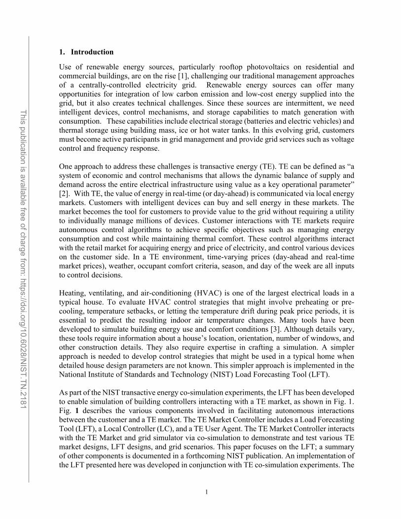
Use of renewable energy sources, particularly rooftop photovoltaics on residential and commercial buildings, are on the rise [1], challenging our traditional management approaches of a centrally-controlled electricity grid. Renewable energy sources can offer many opportunities for integration of low carbon emission and low-cost energy supplied into the grid, but it also creates technical challenges. Since these sources are intermittent, we need intelligent devices, control mechanisms, and storage capabilities to match generation with consumption. These capabilities include electrical storage (batteries and electric vehicles) and thermal storage using building mass, ice or hot water tanks. In this evolving grid, customers must become active participants in grid management and provide grid services such as voltage control and frequency response. One approach to address these challenges is transactive energy (TE). TE can be defined as “a system of economic and control mechanisms that allows the dynamic balance of supply and demand across the entire electrical infrastructure using value as a key operational parameter” [2]. With TE, the value of energy in real-time (or day-ahead) is communicated via local energy markets. Customers with intelligent devices can buy and sell energy in these markets. The market becomes the tool for customers to provide value to the grid without requiring a utility to individually manage millions of devices. Customer interactions with TE markets require autonomous control algorithms to achieve specific objectives such as managing energy consumption and cost while maintaining thermal comfort. These control algorithms interact with the retail market for acquiring energy and price of electricity, and control various devices on the customer side. In a TE environment, time-varying prices (day-ahead and real-time market prices), weather, occupant comfort criteria, season, and day of the week are all inputs to control decisions. Heating, ventilating, and air-conditioning (HVAC) is one of the largest electrical loads in a typical house. To evaluate HVAC control strategies that might involve preheating or pre-cooling, temperature setbacks, or letting the temperature drift during peak price periods, it is essential to predict the resulting indoor air temperature changes. Many tools have been developed to simulate building energy use and comfort conditions [3]. Although details vary, these tools require information about a house’s location, orientation, number of windows, and other construction details. They also require expertise in crafting a simulation. A simpler approach is needed to develop control strategies that might be used in a typical home when detailed house design parameters are not known. This simpler approach is implemented in the National Institute of Standards and Technology (NIST) Load Forecasting Tool (LFT). As part of the NIST transactive energy co-simulation experiments, the LFT has been developed to enable simulation of building controllers interacting with a TE market, as shown in Fig. 1. Fig. 1 describes the various components involved in facilitating autonomous interactions between the customer and a TE market. The TE Market Controller includes a Load Forecasting Tool (LFT), a Local Controller (LC), and a TE User Agent. The TE Market Controller interacts with the TE Market and grid simulator via co-simulation to demonstrate and test various TE market designs, LFT designs, and grid scenarios. This paper focuses on the LFT; a summary of other components is documented in a forthcoming NIST publication. An implementation of the LFT presented here was developed in conjunction with TE co-simulation experiments. The



.2181

2

co-simulation experiment connects the TE Market Controller to wholesale market prices and a residential electric grid sited in Tucson Arizona. GridLAB-D [4] was used as the electric grid simulator, implementing the IEEE-8500 reference grid [5] with 1977 residential house models, having different thermal characteristics and thermal comfort requirements.

The LFT is an integral part of the TE co-simulation. The main objective of the LFT is to learn from observation and predict the next-day’s hourly electrical energy consumption and indoor temperature setpoint profiles for residential house models implemented in GridLAB-D. Realizing the objective of the LFT requires intelligent learning and control algorithms to manage cost and comfort while adapting to changing weather conditions and the price of electricity. Resulting control actions include shifting the heat pump operation schedule via setpoint temperature adjustments (e.g., pre-cooling when the price is low). The LFT comprises two main components, a Learning Algorithm (LA) and a Load Forecasting Algorithm (LFA), interacting with TE Market via the TE User Agent and the GridLAB-D simulation environment via an LC. The LA is responsible for learning key thermal parameters of a lumped capacitance model using output from GridLAB-D simulation (indoor temperature and heat pump power consumption) and historical weather data for Tucson Arizona (outdoor temperature and solar irradiance). The output of the LA is used as an input to the LFA. The LFA is responsible for predicting the hourly energy consumption and indoor temperature setpoint profile of a residential house, using the day-ahead price of electricity, forecast weather conditions, and customer’s thermal comfort requirements. The forecast weather conditions were obtained from

Fig. 1. Interaction of the components in TE Market Controller with the TE Market and the GridLAB-D simulation environment



.2181

3

historical data for Tucson Arizona. A forecast of plug-loads was obtained from generated performance information from GridLAB-D. In this study, it was assumed that the house models in GridLAB-D represented the performance of actual houses. Considering this assumption, GridLAB-D was used to generate performance information such as indoor temperature, plug-loads, heat pump power consumption, and the overall heat transfer conductance (UA) of all IEEE-8500 residential house models. The generated performance data were used to:

1. Tune various parameters of a learning algorithm described in Sec. 2.; and 2. Help a load forecasting algorithm to predict the next-day’s total electrical energy

demand and indoor temperature setpoint profiles described in Sec. 3. The following sections provide a detailed description of the LFT components, the LA and LFA.

Learning Algorithm

Using parameter optimization, the LA learns thermal parameters of a residential house by minimizing the error between generated indoor temperature from GridLAB-D and the output of the lumped capacitance model. The lumped capacitance model forecasts the indoor temperature as a function of key thermal parameters, heat pump energy, solar heat gain, heat gain from plug-loads, and outdoor air temperature. 2.1. Lumped Capacitance Model The LA uses a first-order lumped capacitance model described in [2] to predict the interior air temperature of the house models in GridLAB-D. The houses in the IEEE-8500 grid model, implemented in GridLAB-D, are assumed to be a single control volume with a uniform indoor temperature. The first-order lumped capacitance model used to forecast the indoor temperature is given by Eq. (1.1)

expsol hp l sol hp li

q q q q q q tT T T TUA UA τ∞ ∞

+ + + + = + + − − −

(1.1)

where: T∞ is the outside ambient dry-bulb temperatures, °C; qsol is the total solar heat gain added to the house, W; qhp is the rate of heat generated by the heat pump (thermal energy), W. The value of qhp is negative for the cooling season; ql is the rate of heat generated inside the house by the internal loads, W; Ti is the initial indoor temperature, °C; UA is the overall heat transfer conductance, W/K; τ is the building time constant, h; and t is time.



.2181

4

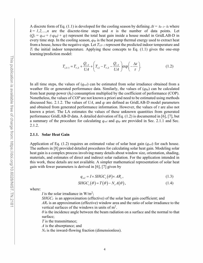
A discrete form of Eq. (1.1) is developed for the cooling season by defining Δt = tk+1- tk where k = 1,2,…,n are the discrete-time steps and n is the number of data points. Let (Qc = qsol + (-qhp) + ql) represent the total heat gain inside a house model in GridLAB-D in every time step. In the cooling season, qhp is the heat pump thermal energy used to extract heat from a house, hence the negative sign. Let Ti,k+1 represent the predicted indoor temperature and Ti the initial indoor temperature. Applying these concepts to Eq. (1.1) gives the one-step learning/prediction model:

, ,, 1 , , , expc k c k

i k k i k k

Q Q tT T T TUA UA τ+ ∞ ∞

∆ = + + − − −

. (1.2)

In all time steps, the values of (qsol) can be estimated from solar irradiance obtained from a weather file or generated performance data. Similarly, the values of (qhp) can be calculated from heat pump power (hp) consumption multiplied by the coefficient of performance (COP). Nonetheless, the values of COP are not known a priori and need to be estimated using methods discussed Sec. 2.1.2. The values of UA, and ql are defined as GridLAB-D model parameters and obtained from generated performance information. However, the values of τ are also not known a priori. The LA estimates the values of these unknown quantities from generated performance GridLAB-D data. A detailed derivation of Eq. (1.2) is documented in [6], [7], but a summary of the procedure for calculating qsol and qhp are provided in Sec. 2.1.1 and Sec. 2.1.2. 2.1.1. Solar Heat Gain Application of Eq. (1.2) requires an estimated value of solar heat gain (qsol) for each house. The authors in [8] provided detailed procedures for calculating solar heat gain. Modeling solar heat gain is a complex process involving many details about window size, orientation, shading, materials, and estimates of direct and indirect solar radiation. For the application intended in this work, these details are not available. A simpler mathematical representation of solar heat gain with fewer parameters is derived in [6], [7] given by

( )sol e eq I SHGC ARθ= × × , (1.3)

( ) ( ) ( )e eSHGC T N Aθ θ θ= − , (1.4) where:

I is the solar irradiance in W/m2; SHGCe is an approximation (effective) of the solar heat gain coefficient; and ARe is an approximation (effective) window area and the ratio of solar irradiance to the vertical surfaces of the windows in units of m2. θ is the incidence angle between the beam radiation on a surface and the normal to that surface; T is the transmittance; A is the absorptance; and Ne is the inward-flowing fraction (dimensionless).



.2181

5

The parameters in Eq. (1.3) and Eq. (1.4) capture the effects of window size and orientation, shading, and the fraction of direct or diffuse solar radiation. The values of these parameters can be learned from generated performance information by GridLAB-D, eliminating the user’s need for detailed custom configuration or prior knowledge of the parameters. The values of SHGCe and ARe for each house are found using multi-objective optimization described in Sec. 3. 2.1.2. Heat Pump Thermal Energy for Learning As previously mentioned, application of Eq. (1.2) requires the values of the heat pump’s thermal energy (qhp). The capacity of a heat pump to generate thermal energy is given by

hp hpq P COP= × , (1.5) where, Php is the heat pump power (W) and COP is the coefficient of performance (dimensionless). COP is defined as the ratio of thermal energy added to or removed from a system and the amount of electric power used to perform the required work. It is a strong function of the outdoor temperature. As an example, the values of COP as a function of outdoor temperature for a two-stage air-source heat pump from the NIST Net-Zero Energy Residential Test Facility (NZERTF) [9], [10] are shown in Fig. 2.

Fig. 2. The COP and regression models of a two-stage air-source heat pump as a function of outdoor temperature in the cooling season



.2181

6

COP can be approximated by a first or a second-order polynomial fit to the NZERTF heat pump’s coefficient of performance data, as shown in Fig. 2. A second-order polynomial model can provide a better fit, but for simplicity of implementation, we used the first-order approximation (denoted as COPe)

e e eCOP m T b∞= + , (1.6) where me is the slope in (1 ℃⁄ ), be is the intercept (dimensionless), and T∞ is the outdoor temperature in ℃. Substituting Eq. (1.6) into Eq. (1.5) gives us

( ).

ehp hp

ehp e

q P COP

m T bP ∞

×

× +

=

= (1.7)

Substituting Eq. (1.3) and Eq. (1.7) into Eq. (1.2) to replace qsol and qhp gives the updated one-step learning/prediction model:

( ) ( )( )

( ) ( )( )

,, 1 ,

,, , exp

e e e e l kk ki k k

e e e ek

hp

h l kpk ki k

e

I SHGC AR m T b qT T

UAI SHGC AR m T b q tT T

U

P

P

A τ

∞

+ ∞

∞

∞

× × − × + += +

× × − × + + ∆ + − − −

(1.8)

Application of Eq. (1.8) requires estimated values of SHGCe, ARe, me, be, and τ (denoted as τe). 2.1.3. Estimating Solar Heat Gain, COPe, and Thermal Time Constant To estimate key parameters of solar heat gain (ARe, Ne), thermal time constant (τe), and the coefficient of performance (me, be), we used an optimization algorithm described in [6], [7]. The optimization algorithm utilizes Eq. (1.8) to learn these effective parameters from generated performance data from GridLAB-D over a 3-day training window. The 3-day training window provided sufficient accuracy, as measured by relative root mean square error (% RMSE) statistics shown in Fig. 4, because the daily variation in solar irradiance and outdoor temperature were minimal for the historical weather data used in this study. In general, a 1-day training window would not be sufficient because the prediction accuracy can be highly influenced by the solar irradiance variability from one day to the next. For example, if the parameters were learned on a cloudy day and applied to a sunny day, the model over-predicted the temperature. The model under-predicted the temperature when the opposite was true. The objective function for the optimization algorithm is defined as the sum of squared error (SSE) between the generated indoor temperature from GridLAB-D (Ts) and the predicted temperature (Ti) obtained from Eq.(1.8). The objective function can be expressed as



.2181

7

( ) 2

2, , , ,e e e e e s if AR N m b T Tτ = − , and (1.9)

the optimization problem becomes

( ), , , ,min , , , ,

10 11 1

11 104

e e e e ee e e e eAR N m b

e

e

e

e

e

f AR N m b

ARNm

b

ττ

τ

≤ ≤ ∞≤ ≤

− ≤ ≤≤ ≤ ∞≤ ≤

, (1.10)

where the units of ARe is m2, Ne is dimensionless, me is 1 ℃⁄ , be is dimensionless, and τe is h. The bounds of the Ne are [0, 1] because it only represents the fraction of the solar irradiance absorbed into the interior spaces. To ensure that for every unit change in the outdoor temperature, there is a maximum of one unit change in the estimated value of the COPe, the bounds of me are set to [-1, 1]. The lower bounds of the ARe and be are set to 1 for numerical stability, but their upper bounds can float because they are not known a priori. For numeric stability, we set the lower bound of τe to 1 h and its upper bound to 104 h. The upper bound for τe was arbitrarily set to the estimated value of the thermal time constant of the NZERTF at NIST in Gaithersburg, Maryland [7]. The NZERTF is a four-bedroom single-family house on the campus of NIST [11], [12]. We assume that the estimated time constant (τe) of the NZERTF represents the highest practical time constant of a very well-insulated residential house with a significant thermal mass capacity. We used the MATLAB non-linear optimization algorithm (fmincon) with its default interior-point algorithm to solve the optimization problem in Eq. (1.10) subject to the given constraints. Fig. 3 shows the simulated indoor air temperature from GridLAB-D and the predicted indoor air temperature, using Eq. (1.10), of a randomly selected house over the 3-day training window. For visual clarity, the top and middle subplots show the moving average of the simulated and predicted air temperature, where each average value is calculated over a sliding window of length 30 min. The bottom subplot shows the simulated and predicted indoor temperature profiles over 2 h window.



.2181

8

Fig. 3. Comparisons between simulated indoor air temperature from GridLAB-D and predicted indoor air temperature from optimization Eq. (1.10) We used % RMSE statistics to describe the goodness of fit and characterize the performance of the LA described in Eq. (1.10). Fig. 4 shows the % RMSE and the average % RMSE of



.2181

9

predicted indoor temperature and simulated indoor temperature in GridLAB-D for all house models. The maximum % RMSE statistic over the 3-day training data set is 1.78 %.

Fig. 4. The % RMSE and average error between predicted and simulated indoor air temperature for all houses, using Eq. (1.10) Estimate of me and be parameters are used in Eq. (1.6) to calculate the COPe of heat pumps in GridLAB-D. Fig. 5 shows the of COPe of heat pumps for all house models in GridLAB-D over the 3-day training window, where the values are in minutes.



.2181

10

Fig. 5. The effective coefficient of performance over the 3-day training window for all house models in GridLAB-D from July 4th to July 7th

As shown in Fig. 5, the maximum value of the COPe is approximately 3.3 at night when the outdoor temperature is cooler, and its minimum value is 2 when the outdoor temperature is hotter.

Load Forecasting Algorithm

As previously mentioned, LFA is another critical component of the LFT. The main objectives of the LFA are to predict the next day’s heat pump energy consumption of a residential house and generate an indoor temperature setpoint profile. We focus on developing intelligent control strategies using the day-ahead price of electricity and customer comfort preferences to achieve these objectives. As mentioned in Sec. 2, HVAC (heat pump) is the most significant electrical load in a typical home; therefore, it can substantially impact the overall energy consumption and cost. Our goal is to reduce the cost of operating the heat pump while maintaining thermal comfort. We used an optimization algorithm to look ahead using the day-ahead price of electricity and a customer’s thermal comfort preferences to achieve this goal. This section defines an optimization problem and uses a linear integer optimization algorithm to generate heat pump control actions, using the lumped capacitance model given in Eq. (1.8) to predict the Ti for the next day. Inputs for the LFA, including forecast data needed for the LFA are given in Table 1.



.2181

11

Table 1. Input Data Needed for Predicting the Heat Pump Energy Consumption and Indoor Temperature Setpoint Profile

Optimization algorithm inputs Description (in context of current research) Forecast solar irradiance (W/m2) Solar irradiance taken from weather file, recorded

historical measurements data for Tucson Arizona. Plug-loads (W) and the overall heat transfer conductance UA (W/K)

The values for forecast plug-loads taken from the performance information data generated in GridLAB-D for the same day as the predicted load.

Forecast of outside dry-bulb temperature, T∞ (°C)

This data taken from a weather file, recorded historical measurements data for Tucson Arizona.

Forecast of day-ahead price of electricity

The day-ahead price of electricity was obtained from the market-clearing prices of California Independent System Operator (CAISO) for Tucson, Arizona.

Forecast of heat pump electrical power consumption (Phpe) for the cooling season.

The Phpe (W) values for the cooling season are obtained from Eq. (1.11). Eq. (1.11) was derived from a linear regression fit to simulated heat pump’s power consumption from GridLAB-D.

Effective parameters: ARe (m2), Ne (dimensionless), τe (h), me (1/°C), and be (dimensionless).

Effective parameters are obtained from LA described in Sec. 2.

Customer preferences such as indoor temperature setpoint (Tsp) (°C) and offset_limit (°C).

The offset_limit is the maximum temperature rise or minimum temperature fall from a given setpoint temperature (Tsp) [4].

The angle of incidence cos(θ) for solar irradiance.

The angle of incidence is calculated from geographical location of a house under consideration. A detailed explanation of cos(θ) is given [13] and an implemented example in [6], [7].

A schematic representation of the LFA process for obtaining the next-day hourly heat pump energy consumption and setpoint temperature profile is shown in Fig. 6.

Fig. 6. A schematic representation of the LFA processes for predicting heat pump load for the next day



.2181

12

The LFA utilizes a multi-objective optimization problem and constraints to forecast heat pump control actions. The optimization problem in the LFA is formulated such that the solver selects control actions to minimize the overall value of the objective function (Eq. (1.12)) while satisfying the constraints. The output of the optimization function is a vector of heat pump control actions for the next 24 hours. These control actions are directly related to the hourly heat pump energy consumption of a residential house model represented by Eq (1.8) because the optimization problem is formulated in such a way that the heat pump operation is the control variable. The predicted hourly heat pump energy consumption for a residential house model is summed and added to its baseline load (plug-loads and water heater load where applicable) from GridLAB-D to calculate the total energy demand for tomorrow. The same procedure is applied to all 1977 house models. The total energy demand for all residential houses is assembled into a vector of House Energy Demand in LFT as shown in Fig. 6. The House Energy Demand is communicated to the market to pre-purchase electricity. The other output of the LFT is predicted indoor temperature setpoint profile from LFA to GridLAB-D via the LC. The LFA is designed to output an optimal or an integer feasible solution. The LFA is terminated after it finds an optimal policy or exceeds a pre-defined stopping criterion of 3 min maximum timeout limit. The stopping criterion was imposed on the optimization solver discussed in Sec. 3.2. The LFA was implemented in a desktop computer with Intel® Xeon® CPU E5-1630 v3 3.7 GHz processor and 16 GB of RAM. Recall that in Sec. 2.1.2, the capacity of a heat pump to generate thermal energy was defined as the product of heat pump power consumption (Php) and the coefficient of performance (COP) given by Eq. (1.5). In Sec. 2.1.3, the values of Php, for all house models in GridLAB-D, were known and we used the LA to estimate the values of the COPe from observation. However, in a realistic scenario that requires forecasting the next day’s indoor temperature, the values of Php are not known a priori. Therefore, there is a need for a model to predict Php (denoted as Phpe) and utilize Eq. (1.8) to predict Ti. Section 3.1 describes a procedure for identifying parameters of a regression model to forecast Phpe as a function of the outdoor temperature. 3.1. Heat Pump Power for LFA To predict Phpe as a function of outdoor temperature we need a model that is simple to implement and provides accurate estimate of the heat pump power consumption. It is known that heat pump power consumption is a strong function of the outdoor temperature. Using this information, we used a simple first-order linear regression model and estimated its slope and intercept from generated performance data; that is, heat pump power consumption data from GridLAB-D as a function of the outdoor temperature, as shown in Fig. 7.



.2181

13

Fig. 7. Estimating the parameters of the first-order linear regression model using heat pump power consumption of a residential house model in GridLAB-D versus the outdoor temperature, and its residual plot

We performed similar analysis, as shown in Fig. 7, to identify the parameters of first-order linear regression models for all house models represented by Eq. (1.8) in this study. Using the slope and intercept of regression estimates, we can calculate the electrical power consumption (Phpe) of a heat pump as a function of outdoor temperature by

,hpe hp hpP m T b∞= × − (1.11) where, Phpe is the electrical power in (W), mhp (W/°C) and bhp (W) are the slope and intercept of the linear regression model, and T∞ is the outdoor temperature in °C. The RMSE statistics for estimating the slope and intercept of Eq. (1.11) for all house models is given in Fig. 8.



.2181

14

Fig. 8. The RMSE and average error statistics for estimating Phpe from generated performance information, representing all house models in GridLAB-D

As can be seen from Fig. 8, the values of RMSE suggest that our linear model provides a reasonable estimate of the heat pump power consumption as a function of outdoor temperature.



.2181

15

3.2. Objective Function and Constraints The objective function of the LFA is formulated in such a way that it minimizes cost while maintaining thermal comfort. The mathematical representation of the objective function is given in Eq. (1.12), describing the multi-objective optimization problem

[ ]

( ) ( )11 1 12,min 1

kk SP k hpe k kk nT T u P w xλ λ

−− − −∈⋅ − + − ⋅ ⋅ ⋅ , (1.12)

where: k represents the discrete simulation time steps [min]; n represents the forecast horizon 1440 [min]. For speed and stability of the optimization

solver, the forecast horizon has been divided into 144 bins. Simulation data in each bin represents 10 min of the forecast horizon;

u represents the binary decision variable [dimensionless], and at each simulation time step, it is defined as

1, if the heat pump operating0, otherwise;

u ∈

Phpe represents the electrical power associated with the operation heat pump [W], given by Eq. (1.11);

w represents heat pump power normalization factor [1°C/W]. The normalization factor is defined as 1°C/max(𝑃𝑃ℎ𝑝𝑝𝑝𝑝), where Phpe is given by Eq. (1.11);

λ is a value between 0 and 1, representing the relative dominance between comfort and cost [dimensionless, varies between house models];

Tk represents the predicted indoor temperature at each simulation time step k [℃] obtained from Eq. (1.2);

Tsp represents the setpoint temperature [℃]. Setpoint temperatures are obtained from GridLAB-D;

x represents the vector of normalized values of the price of electricity [dimensionless] and is given by

( ) , [ , ]DADA

DA

px p k nP

= ∀ ∈ , where DAP is the day-ahead price of electricity, and DAP is

the average value of day-head price of electricity in [$/kWh]. Heat pump power consumption (Phpe) and price (x) were normalized to keep the terms of the objective function from dominating the solution. The DAP and DAP values for electricity were obtained from two weeks (June 23rd to July 7th, 2017), using the day-ahead price of electricity for Tucson, Arizona described in Table 1, as shown in Fig. 9.



.2181

16

Fig. 9. Two weeks of the day-ahead price of electricity for Tucson, Arizona from Jun 23rd to July 7th, 2017 To obtain values of λ used in Eq. (1.12), we used a linear mapping from the GridLAB-D house comfort parameters described in [14] to λ, where the comfort parameter represents a homeowner’s desire for comfort versus saving money. The value of λ is between 0 (most cost-conscious) and 1 (most comfort-conscious). The objective function defined in Eq. (1.12) contains a non-linear term, the absolute value of (Tk - Tsp). In its current form, we cannot solve it using a linear optimization method. Applying a linear optimization method requires that the objective function and all its constraints are expressed in linear form. To linearize the objective function, the absolute value term given in Eq. (1.12) is replaced with a variable Z, and two additional linear constraints are added to the problem definition. The linear constraints replacing the absolute value term of the objective function are expressed as

( )

1

1,k SP k

k SP k

T T ZT T Z

−

−

− ≤

− − ≤ (1.13)

where Z has a unit of [°C]. In addition, Tk is constrained as

klb T ub≤ ≤ , (1.14)



.2181

17

where lb and ub represent the lower and upper bound temperatures limits [℃]. The lb and ub temperature values are different for each house model, calculated by Tsp ± offset_limit. The offset_limit represents the temperature rise from a setpoint to the maximum allowed temperature specified by a customer, or the temperature reduction to a minimum temperature. The range of offset_limit is 1.67 ℃ < offset_limit < 2.78 ℃. Substituting the Z term and adding the constraints to Eq. (1.12) gives us the linear form of the objective function and its constraints as

[ ]( ) ( )

( )

11 1 1 12,

1

1

min 1

:kk k hpe k kk n

k SP k

k SP k

k

Z u P w x

Subject toT T Z

T T Zlb T ub

λ λ−− − − −∈

−

−

⋅ + − ⋅ ⋅ ⋅

− ≤

− − ≤

≤ ≤

. (1.15)

The optimization problem in Eq. (1.15) was modeled as a pure integer problem in YALMIP [14], a modeling and optimization toolbox for MATLAB. The integer optimization model was solved using the linear integer programming algorithm (intlinprog) from MATLAB with its default settings except for the MaxTime (stopping criterion in Fig. 6) parameter. MaxTime parameter is the maximum time that intlinprog runs to find a solution. The default value for MaxTime is 7200 s, which can prohibit a simulation of over 1900 house models from being completed in a reasonable time. In this study, the value for MaxTime was set to 180 s. Fig. 10 shows the daily predicted heat pump energy demand (top subplot) and total energy demand (bottom subplot) for all residential house models and their average energy use across all houses for tomorrow.



.2181

18

Fig. 10. The daily predicted heat pump energy demand and total energy demand and their average energy use across all houses for tomorrow

The daily total energy demand of a residential house model is the sum of hourly predicted heat pump energy demand from the LFA, plug-loads, and water heater (where applicable). The energy consumptions for the plug-loads and water heater were obtained from generated performance data from GridLAB-D. Note that not all house models in GridLAB-D have an electric water heater unit. The daily cost of energy consumption is calculated as the sum of hourly energy demand for tomorrow multiplied by the hourly day-ahead price of electricity for July 7th, as shown in Fig. 9. The objective of the LFA is to minimize cost but maintain thermal comfort. To avoid higher cost the LFA may choose to pre-cool the indoor temperature near the lb limit when the cost of electricity is lower. Conversely, the LFA may choose to let the indoor temperature drift up to the ub limit when electricity is more expensive. The LFA achieves its objective by controlling the heat pump operation. To demonstrate the LFA’s effectiveness, we selected three different houses, having maximum (top subplot), minimum (middle subplot), and average (bottom subplot) integrated hourly heat pump energy demand, as shown in Fig. 11. The LFA avoids the peak price of electricity by shifting the heat pump’s operation to other times when the price is cheaper.



.2181

19

Fig. 11. A one-day profile of hourly predicted heat pump energy demand and the day-ahead price of electricity for July 7th.

As mentioned before, heat pump control actions in the LFA resulted in predicted indoor temperature profiles for all houses, which are used as adjusted setpoint temperatures input to GridLAB-D. GridLAB-D uses the adjusted setpoint temperatures to control its internal heat pump operation. The predicted indoor temperature profiles and predicted heat pump energy demand for the houses shown in Fig. 11 are given in Fig. 12.



.2181

20

Fig. 12. The impact of heat pump energy consumption on indoor temperature profiles generated by the LFA

As shown in Fig. 12, the LFA maintains the indoor temperature within the ub and lb constraints. The LFA is managing the indoor temperature by generating heat pump control actions to reduce cost by avoiding the peak price of electricity and maintaining thermal comfort. To verify the resulting energy savings of the LFA, we compared the predicted heat pump energy demand with the simulated heat pump energy demand from GridLAB-D on July 7th, as shown in Fig. 13.



.2181

21

Fig. 13. Simulated heat pump energy demand from GridLAB-D and predicted heat pump energy demand from LFA for all houses

As shown in Fig. 13, the LFA reduced the energy demand, shifting the histogram to the left with a resulting 9.4 % energy savings (on average) compared to the simulated heat pump energy demand from GridLAB-D. The heat pump energy savings were realized for all houses except for four, where the predicted energy demand exceed the simulated energy demand by less than 5 %, as shown in Fig. 14.



.2181

22

Fig. 14. Percent difference in energy consumption of simulated heat pump energy demand from GridLAB-D minus the predicted heat pump energy demand from the LFA

To verify the resulting cost savings of the LFA, we compared the cost of predicted heat pump energy demand with the cost of simulated heat pump energy demand from GridLAB-D on July 7th, as shown in Fig. 15. The cost of energy consumption is calculated as the sum of hourly heat pump energy demand multiplied by the hourly day-ahead price of electricity for July 7th, as shown in Fig. 9.



.2181

23

Fig. 15. The cost of predicted heat pump energy demand from LFA and simulated heat pump energy demand from GridLAB-D

As shown in Fig. 15, the LFA produced 19.4 % in cost savings (on average) compared to the simulated heat pump energy demand from GridLAB-D. The cost savings were realized for all houses because the LFA avoided the peak price of electricity as shown in Fig. 11. The percent difference in cost of predicted heat pump energy demand and simulated heat pump energy demand from GridLAB-D is shown in Fig. 16.



.2181

24

Fig. 16. Percent difference in cost of simulated heat pump energy demand minus the cost of predicted heat pump energy demand

The results of additional comparisons, using the output of the LFT on energy consumption and voltage stability are reported in [15].

Conclusion and Future Work

Customers and transactive energy market managers may rely on load forecasting algorithms to purchase or sell energy in a forward market environment, using day-ahead and real-time pricing structures. Accurate load forecasting becomes necessary when a local controller interacts with an electricity market environment to purchase energy for future use or an aggregator who can bid energy for sale into the electricity markets. This report introduced the LFT that estimated next day energy consumption for all residential house models in GridLAB-D. The LFT achieved its objectives by utilizing the LA and the LFA described in Sec. 2 and Sec. 3, respectively. The LA estimated key parameters of residential house models given by Eq. (1.8), such as thermal time constant, solar heat gain coefficient, effective window area, and heat pump’s coefficient of performance using generated performance information and historical weather data. The LFA utilized a multi-objective optimization problem to minimize cost and maintain thermal comfort, resulting in average energy savings of 9.4 % and average cost savings of 19.4 % compared to simulated heat pump energy demand from GridLAB-D. The LFA used the residential house model given by Eq. (1.8) to forecast the next



.2181

25

day’s indoor temperature by manipulating heat pump operation. The LA and LFA were applied to 1977 residential house models. All components of the LFT were implemented standalone, resulting in predicted indoor temperature profiles and predicted total energy demand. The predicted indoor temperature profiles, for each house, was provided as a file input to GridLAB-D. GridLAB-D used these temperature profiles as adjusted thermostat setpoints for controlling the operation of the heat pumps in each house. Future work might entail integrating the LFT in a real-time simulation with GridLAB-D.



.2181

26

References

[1] U. S. D. of Energy, “Annual Energy Outlook 2021 with Projection to 2050 Narrative,” 2021. [Online]. Available: https://www.eia.gov/outlooks/aeo/pdf/AEO_Narrative_2021.pdf.

[2] The GridWise Architecture Council, “GridWise Transactive Energy Framework Version 1.0,” 2015. [Online]. Available: https://www.gridwiseac.org/pdfs/te_framework_report_pnnl-22946.pdf.

[3] IBPSA-USA, “Best Directory | Building Energy Software Tools.” http://www.buildingenergysoftwaretools.com/ (accessed Aug. 15, 2015).

[4] “GridLAB-D Simulation Software,” 2011. [Online]. Available: http://www.gridlabd.org.

[5] D. Holmberg et al., “NIST Transactive Energy Modeling and Simulation Challenge Phase II,” 2019. doi: https://doi.org/10.6028/NIST.SP.1900-603.

[6] F. Omar, S. T. Bushby, and R. D. Williams, “A self-learning algorithm for estimating solar heat gain and temperature changes in a single-Family residence,” Energy Build., vol. 150, 2017, doi: 10.1016/j.enbuild.2017.06.001.

[7] F. Omar and S. T. Bushby, “A Self-Learning Algorithm for Temperature Prediction in a Single Family Residence,” NIST Tech. Note 1891, 2015, doi: http://dx.doi.org/10.6028/NIST.TN.1891.

[8] “Chapter 15. Fenestration,” in ASHRAE Handbook: Fundamentals, ASHRAE, 2013, p. 13.

[9] W. V. Payne, “NZERTF’s Heat Pump Capacity Outputs,” Private Communications, National Institute of Standards and Technology, MD, 2013. [Online]. Available: https://www.nist.gov/people/vance-wm-payne.

[10] M. Davis et al., “Monitoring Techniques for the Net-Zero Energy Residential Test Facility,” NIST Technical Note 1854, 2014.

[11] H. Fanney et al., “Net-zero and Beyond! Design and Performance of NIST’s Net-zero Energy Residential Test Facility,” Energy Build. 101, pp. 95–109, 2015, doi: http://dx.doi.org/10.1016/j.enbuild.2015.05.002.

[12] F. Omar and S. T. Bushby, “Simulating Occupancy in The NIST Net-Zero Energy Residential Test Facility,” NIST Tech. Note 1817, 2013, doi: https://doi.org/10.6028/NIST.TN.1817.

[13] J. A. Duffie and W. A. Beckman, “Solar Radiation,” in Solar Engineering of Thermal Processes, 3rd ed., Wiley, 2006, pp. 3–17.

[14] J. Lofberg, “YALMIP : a toolbox for modeling and optimization in MATLAB,” in 2004 IEEE International Conference on Robotics and Automation (IEEE Cat. No.04CH37508), 2004, pp. 284–289, doi: 10.1109/CACSD.2004.1393890.

[15] D. G. Holmberg, F. Omar, and T. P. Roth, “Comparison of Two Approaches for Managing Building Flexibility Using Energy Market Prices,” NIST Tech. Note xxxx, 2021.



.2181