Embed Size (px)
Citation preview
Lloret-Cabot, M., Wheeler, S. J. and Sánchez, M. (2017) A unified
mechanical and retention model for saturated and unsaturated soil
behaviour. Acta Geotechnica, 12(1), pp. 1-21. (doi:10.1007/s11440-016-
0497-x)
This is the author’s final accepted version.
There may be differences between this version and the published version.
You are advised to consult the publisher’s version if you wish to cite from
it.
http://eprints.gla.ac.uk/150055/
Deposited on: 18 October 2017
Enlighten – Research publications by members of the University of Glasgow
http://eprints.gla.ac.uk

1
Full paper contribution to ACTA GEOTECHNICA
8528 words
21 Figures and 4 Tables
-------------------------------------------------------------------------------------------------------
A unified mechanical and retention model for saturated and
unsaturated soil behaviour
Author 1
Martí Lloret-Cabot, Ph.D
Faculty of Engineering and Built Environment, University of Newcastle,
Newcastle, Australia
Formerly Universities of Strathclyde and Glasgow, Glasgow, UK
Author 2
Simon J. Wheeler, Prof
School of Engineering, University of Glasgow, Glasgow, UK
Author 3
Marcelo Sánchez, A/Prof
Department of Civil Engineering, Texas A & M University, Texas, USA
Formerly University of Strathclyde, Glasgow, UK
Corresponding author
Martí Lloret Cabot
Faculty of Engineering and Built Environment
University of Newcastle
Callaghan, Building EA
NSW 2308
Australia
Tel. +61 2 4921 5660

2
ABSTRACT
The coupled mechanical and water retention elasto-plastic constitutive model of
Wheeler, Sharma and Buisson (the Glasgow Coupled Model, GCM) predicts unique
unsaturated isotropic normal compression and unsaturated critical state planar surfaces
for specific volume and degree of saturation when soil states are at the intersection of
Mechanical (M) and Wetting Retention (WR) yield surfaces. Experimental results from
tests performed by Sivakumar on unsaturated samples of compacted speswhite kaolin
confirm the existence and form of these unique surfaces. The GCM provides consistent
representation of transitions between saturated and unsaturated conditions, including
the influence of retention hysteresis and the effect of plastic volumetric strains on
retention behaviour, and it gives unique expressions to predict saturation and de-
saturation conditions (air-exclusion and air-entry points respectively). Mechanical
behaviour is modelled consistently across these transitions, including appropriate
variation of mechanical yield stress under both saturated and unsaturated conditions.
The expressions defining the unsaturated isotropic normal compression planar surfaces
for specific volume and degree of saturation are central to the development of a
relatively straightforward methodology for determining values of all GCM parameters
(soil constants and initial state) from a limited number of laboratory tests. This
methodology is demonstrated by application to the experimental data of Sivakumar.
Comparison of model simulations with experimental results for the full set of
Sivakumar’s isotropic loading stages demonstrates that the model is able to predict
accurately the variation of both specific volume and degree of saturation during
isotropic stress paths under saturated and unsaturated conditions.
Keywords: unsaturated soils, saturated soils, constitutive relations, mechanical behaviour, water
retention, suction, saturation, de-saturation, retention hysteresis

3
INTRODUCTION
Wheeler et al. [51] developed a coupled elasto-plastic constitutive model for
unsaturated soils, which represents both mechanical behaviour and water retention
behaviour, including the coupling between them. The model, originally presented
solely for isotropic stress states, has subsequently been extended to general stress states
(e.g. Lloret-Cabot et al. [24]) and is referred to hereafter as the Glasgow Coupled Model
(GCM). In the model, a single yield surface represents mechanical behaviour, with
plastic volumetric strains p
vd and plastic deviatoric strains p
qd occurring during
yielding on this surface. Two other yield surfaces represent water retention behaviour,
with plastic changes of degree of saturation p
rdS occurring during yielding on either
of these surfaces. Coupled movements of the three yield surfaces represent the influence
of plastic changes of degree of saturation on mechanical behaviour and the influence of
plastic volumetric strains on water retention behaviour.
In this paper it is shown that the GCM predicts unique expressions for specific volume
v and degree of saturation Sr for stress states involving simultaneous mechanical
yielding (occurrence of plastic compression) and wetting retention yielding (occurrence
of plastic increases of Sr). These expressions for v and Sr facilitate significantly the
use and interpretation of the model, including determination of model parameter values
from experimental test data.
A major challenge of constitutive models for unsaturated soils is the correct
representation of transitions between unsaturated and saturated conditions. The
challenge of properly modelling such transitions is intimately linked to consistent
consideration of retention hysteresis and to the choice of stress state variables, with
particular difficulties for conventional models expressed in terms of net stresses (excess
of total stress over pore air pressure) and suction (difference between pore air pressure
and pore water pressure), because de-saturation during drying will not occur at zero
suction and subsequent re-saturation on wetting will occur at a different value of
suction. This paper shows how the GCM is able to provide consistent representation of
transitions between unsaturated and saturated states, through the use of non-
conventional stress state variables and proper consideration of retention hysteresis. The
model gives unique expressions to predict saturation and de-saturation conditions,
4
which account for both retention hysteresis and the influence of plastic volumetric
strains on retention behaviour, and it provides consistent modelling of mechanical
behaviour across these transitions.
THE GLASGOW COUPLED MODEL (GCM)
The stress variables used in the GCM are “Bishops’s stress” tensor σij* (sometimes also
called “average soil skeleton stress”, Jommi [19]) and “modified suction” s* . The stress
tensor σij* is similar to the effective stress expression proposed by Bishop in 1959 [4]
but with his weighting factor replaced by the degree of saturation (as suggested in
Schrefler [36]). For the restricted range of stress states that apply in the triaxial test, it
is sufficient to consider only mean Bishop’s stress p* , deviator stress q and modified
suction s* , defined as follows:
* 1r w r a rp p S u S u p S s (1)
31 q (2)
*
a ws n u u ns (3)
where p is mean total stress, uw is pore water pressure, ua is pore air pressure, σ1
and σ3 are, respectively, major and minor principal total stresses and n is porosity.
p and s are mean net stress and matric suction respectively, where p , q and s are
the stress variables used in many more conventional mechanical constitutive models
for unsaturated soils, such as the Barcelona Basic Model (BBM) of Alonso et al. [1].
The stress variables p* , q and s* are work-conjugate with volumetric strain increment
dεv , deviatoric strain increment dεq and decrement of degree of saturation –dSr
respectively (Houlsby [18]).
Elastic components of dεv, dεq and –dSr are given by:
*
*
e
v
dpd
vp
(4)

5
3
e
q
dqd
G (5)
*
*
s
dsdS se
r
(6)
where κ is the elastic swelling index, giving the gradient of elastic swelling lines in
the v:*ln p plane (mechanical behaviour), G is the elastic shear modulus (mechanical
behaviour) and κs is the gradient of elastic scanning curves in the Sr:*ln s plane (water
retention behaviour).
The model includes three yield surfaces in p*:q:s* space: a Mechanical (M) yield
surface to represent mechanical behaviour (originally referred to as the Loading
Collapse (LC) yield surface in Wheeler et al. [51]) and Wetting Retention (WR) and
Drying Retention (DR) yield surfaces to represent water retention behaviour (originally
referred to as, respectively, the Suction Decrease (SD) and Suction Increase (SI) yield
surfaces). Plastic volumetric strains and plastic deviatoric strains occur during yielding
on the M surface, whereas plastic changes of degree of saturation occur during yielding
on WR or DR surfaces. The re-naming of the yield surfaces from the original
terminology used in [51] is to make explicit the fact that the M surface is the only one
of the three describing mechanical yielding (and this can occur during loading, wetting
or drying, see Lloret-Cabot et al. [25]), whereas the other two describe retention
behaviour. This contrasts with the BBM, where both LC and SI yield surfaces represent
mechanical behaviour (Alonso et al. [1]).
The equations of M, WR and DR surfaces are given respectively by:
2 2 * * *
0 0q p p p (7)
* *
1 0s s (8)
* *
2 0s s (9)
where is a soil constant and p0* , s1
* and s2* are hardening parameters defining
the current positions of the M, WR and DR yield surfaces respectively (Figure 1).
6
Equation 7 indicates that constant s* cross-sections of the mechanical yield surface are
elliptical in shape (of aspect ratio ) and the size p0* of these cross-sections does
not vary with s* . Equations 8 and 9 indicate that the WR and DR surfaces form vertical
walls in p*:q:s* space (Figure 1).
Associated flow rules are assumed on all three yield surfaces. This means that yielding
on the M surface alone corresponds to:
2*2
*2
p
v
p
q
d
d and 0p
rdS (10)
where η* = q/p* . Similarly, yielding on the WR surface alone corresponds to:
0p p
q vd d and p
rdS > 0 (11)
and yielding on the DR surface alone corresponds to:
0p p
q vd d and p
rdS < 0 (12)
The hardening law giving movements of the M yield surface includes a direct
component of movement caused by plastic volumetric strain (due to yielding on the M
surface) but also a second (coupled) component of movement caused by any plastic
changes of Sr due to yielding on WR or DR surfaces:
*
01*
0
p p
v r
s s
dp vd dSk
p
(13)
where λ and κ are the gradients of normal compression lines and swelling lines
respectively in the v:*ln p plane for isotropic loading and unloading tests involving no
plastic changes of Sr (such as saturated tests), λs and κs are the gradients of main
wetting/drying curves and scanning curves respectively in the Sr:*ln s plane (see
Figure 2a) for retention tests involving no plastic volumetric strains, and k1 is a
coupling parameter.
Similarly, the hardening law giving movements of the WR or DR yield surfaces includes
a direct component of movement caused by plastic change of Sr (due to yielding on

7
the WR or DR surface) and a second (coupled) component of movement caused by any
plastic volumetric strains due to yielding on the M surface:
p
v
ss
p
rvd
kdS
s
ds
s
ds2*
2
*
2
*
1
*
1 (14)
where k2 is a second coupling parameter. Equation 14 ensures that the movements of
the DR and WR yield surfaces are such that the ratio of *
2s to
*
1s (the spacing of the
DR and WR surfaces when plotted in terms of *ln s ) remains constant:
Rs
s
*
1
*
2 (15)
where R is a soil constant.
The special cases of the hardening laws during yielding on only a single yield surface
(M, WR or DR) are given by inserting the relevant condition from Equation 10, 11 or
12 ( 0p
rdS or 0p
vd ) into Equations 13 and 14.
When the soil reaches a saturated condition ( 1r
S ), further elastic increases of Sr are
prevented (Equation 6 no longer applies for decreases of *s ) and further plastic
increases of Sr are prevented ( 0 p
r
p
v
p
qdSdd replaces Equation 11 for states on
the WR yield surface alone). In addition, the consistency condition on the WR yield
surface is removed, so that the stress state can pass beyond the WR surface. This is
illustrated in Figure 2, with Figure 2a showing water retention behaviour (for conditions
of no plastic volumetric straining), including a saturated point X, and Figure 2b showing
the corresponding positions of the yield curves when the stresses are at point X. While
the soil is saturated, the M yield surface is still operative, and Equation 13 (with
0p
rdS ) recovers the conventional Modified Cam Clay hardening law (Roscoe and
Burland [35]). Also, while the soil is saturated, Equation 14 (with 0p
rdS ) is still used
to determine coupled movements of the WR and DR surfaces caused by plastic
volumetric strain. This represents changes of air entry value caused by plastic
volumetric strain.

8
The model predicts the occurrence of critical states that correspond to the apex of the
elliptical cross-sections of the M yield surface and hence it predicts a unique critical
state line in the q:p* plane:
*pq (16)
The assumption of a unique critical state line in the q:p* plane has been demonstrated
for a range of compacted non-expansive fine grained soils (e.g. Gallipoli et al. [16],
Lloret-Cabot et al. [24]).
DERIVATION AND VALIDATION OF EXPRESSIONS FOR v AND Sr
Isotropic normal compression states
Due to the coupled movements of the yield surfaces, there is a very wide variety of
isotropic stress paths that will ultimately arrive at the intersection between M and WR
surfaces (Point A in Figure 3). For example, if yield occurs first on the M surface, this
will cause a coupled movement of the WR surface, which after a while will typically
bring the WR surface to the stress point. Similarly, if yield occurs first on the WR
surface, this will cause a coupled inward movement of the M surface, which after a
while will typically bring the M surface in to the stress point. More generally, any stress
paths where plastic volumetric strains and plastic increases of Sr occur simultaneously
correspond to this intersection of M and WR surfaces. Inspection of the literature
indicates that this behaviour applies to the majority of published experimental data for
normal compression states. This is because the occurrence of plastic compression
typically observed during isotropic (or one dimensional) loadings at constant suction
reduces porosity and, when such reduction is sufficiently large, irreversible increases
of Sr are also observed, even though suction remains constant during the test (e.g. [8,
10, 13, 14, 22, 28-30, 32-34, 37, 41, 42, 44, 45, 47, 49, 51]). This type of response is
also very often observed in available experimental data showing collapse compression
behaviour on wetting (e.g. [13, 14, 22, 28-30, 32-34, 37, 41, 42, 44, 51]). In this case,
the plastic increases of Sr caused when decreasing suction tend to reduce the stability
of the soil skeleton [51] and this loss of stability may potentially result in volumetric

9
compression [25]. From a theoretical point of view, a proper representation of this
coupling between variations of volumetric strains (mechanical behaviour) and
variations of degree of saturation or suction (retention behaviour) during loading and
wetting paths has been the focus of a large number of constitutive relationships
proposed in the literature (e.g. [1, 3, 9, 12, 13-15, 20, 21, 23-27, 31, 34, 39, 40, 46, 48,
49, 51-53]), because they potentially play a critical role in the geotechnical response of
boundary value problems involving unsaturated soils (e.g. [2, 5-7, 11, 17, 22, 38, 43]).
What can now be shown is that the model predicts unique expressions for v and Sr
for these isotropic normal compression states at the intersection of M and WR surfaces.
Combining Equations 13 and 14 gives the following expressions for p
vd and P
rdS
in terms of the movements of the M and WR yield surfaces:
* *
0 11* *
1 2 0 11
p
v
dp dsd k
v k k p s
(17)
**
012* *
1 2 1 01
s sp
r
dpdsdS k
k k s p
(18)
Equations 4 and 17, for the elastic and plastic components of volumetric strain, can be
combined, in order to give the total volumetric strain increment and hence the total
increment of v :
* **
0 11* * *
1 2 0 11
dp dsdpdv k
p k k p s
(19)
For an isotropic stress state at the intersection between M and WR surfaces ( * *
0p p
and * *
1s s ) and an isotropic stress increment remaining at this intersection ( * *
0dp dp
and * *
1ds ds ), Equation 19 simplifies to:
*
**
1*
**
s
dsk
p
dpdv (20)
where:

10
21
21*
1 kk
kk
(21)
21
1
*
11 kk
kk
(22)
Integration of Equation 20 indicates that the model predicts that values of v for
isotropic normal compression states at the intersection of M and WR yield surfaces are
given by the following unique expression:
**
1
*** lnln skpv (23)
where λ* and *
1k are soil constants given by Equations 21 and 22, and * is an
additional soil constant. Equation 23 represents a planar surface in v:*ln p : *ln s space,
as shown in Figure 4.
A similar procedure for the variation of Sr shows that the model predicts that values
of Sr for isotropic normal compression states at the intersection of M and WR yield
surfaces are given by:
**
2
*** lnln pksS sr (24)
where *
s and *
2k are soil constants given by:
21
21*
1 kk
kk sss
(25)
21
2
*
21 kk
kk ss
(26)
and * is an additional soil constant. Equation 24 represents a planar surface in Sr:
*ln p : *ln s space, as shown in Figure 5.
General states

11
Expressions for v and Sr for any general stress state (see Point B in Figure 3) can now
be derived by considering an elastic stress path from A (coordinates *
0p , 0, *
1s ) to B
(coordinates p*, q, s* ):
** * * * * 0
0 1 1 *ln ln ln
pv p k s
p
(27)
** * * * *
1 2 0 *
1
ln ln lnr s s
sS s k p
s
(28)
Equations 27 and 28 provide general expressions for v and Sr for any stress state (p*,
q, s*) when the current locations of the M and WR yield surfaces are given by *
0p and
*
1s respectively.
For the particular case of isotropic stress states at the intersection between M and DR
surfaces (Point C in Figure 3), *
0
* pp , *
1
* Rss and Equations 27 and 28 give:
* * * * * *
1 1ln ln lnv k R p k s (29)
**
2
**** lnlnln pksRSsssr
(30)
Critical states
The model predicts that critical states can correspond to any points at the apex of the M
yield surface, such as Points D, E and F in Figure 3. In practice, however, it will
normally happen that critical states correspond to the intersection with the WR yield
surface (i.e. Point D in Figure 3), because yielding on the M surface will cause coupled
movement of the WR surface that will be sufficient to bring the WR surface to the stress
point prior to arrival at a critical state.
Expressions for v and Sr for critical states corresponding to the intersection of M and
WR yield surfaces (Point D in Figure 3) can be derived from the general expressions of
Equations 27 and 28 by inserting * *
0 2p p (based on the elliptical shape of constant s*
cross-sections of the M surface) and * *
1s s . This gives:

12
**
1
*** lnln skpv (31)
**
2
*** lnln pksS sr (32)
where * and * are given by:
2ln*** (33)
2ln*
2
** k (34)
Equations 31 and 32 define two unique critical state planar surfaces, in v:*ln p : *ln s
and Sr:*ln p : *ln s spaces respectively. Comparison with Equations 23 and 24 indicates
that these critical state surfaces for v and Sr are predicted to be parallel to the
corresponding normal compression surfaces.
Experimental validation for isotropic normal compression states
Experimental data from the tests of Sivakumar [41] on compacted speswhite kaolin are
used to investigate the validity of the model predictions of unique planar surfaces for v
and Sr for both isotropic normal compressions states and critical states.
Experimental results are taken from 15 constant suction isotropic loading tests
performed by Sivakumar [41] on unsaturated samples at three different values of
suction s (100, 200 and 300 kPa). In each unsaturated test, the isotropic loading was
preceded by an initial equalisation stage, as the sample was wetted from a substantially
higher as-compacted value of suction. In all cases, plastic increases of degree of
saturation occurred during the equalisation stage and plastic volumetric strains and
increases of Sr occurred during the isotropic loading stage, consistent with soil states
at the intersection of M and WR yield surfaces.
Figures 4 and 5 show experimental values of v and Sr from each isotropic loading
unsaturated test that corresponded to soil states at the intersection of M and WR yield
surfaces plotted in v:*ln p : *ln s and Sr:
*ln p : *ln s spaces respectively, together with
the corresponding best-fit planar surfaces obtained by least-squares multiple regression.

13
The gradients and intercepts of these best-fit surfaces gave values for * , *
1k , *
s ,
*
2k , * and * (see Equations 23 and 24), which are listed in Table 1.
A clearer view of the quality of fit shown in the three-dimensional representation
presented in Figure 4 is provided by re-plotting the experimental data and best-fit
surface for v in a pair of orthogonal two-dimensional views in Figure 6, using a form
of plotting where the best-fit surface is reduced to a single straight line in each of the
two views. Figure 7 provides an equivalent representation for Sr . Inspection of Figures
6 and 7 indicates that the two planar surfaces (for v and Sr ) provide excellent fits to
the experimental data.
Experimental validation for critical states
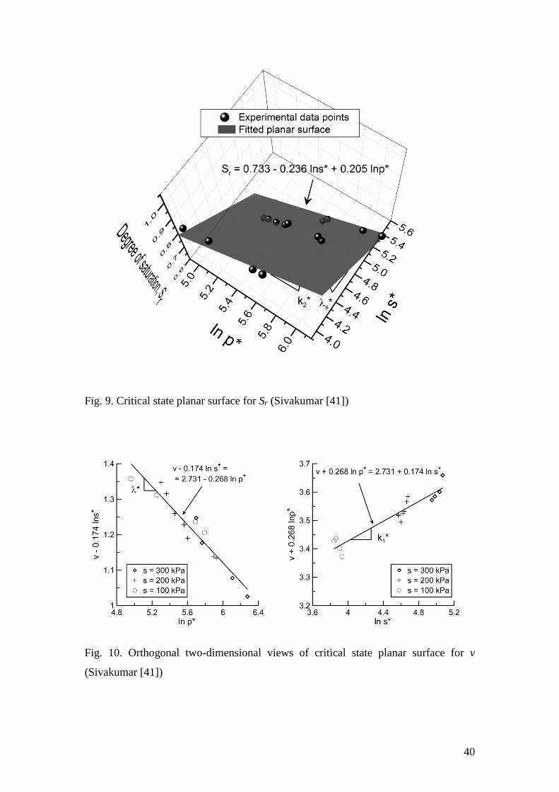
Each of the experimental tests of Sivakumar [41] involved shearing to failure after the
isotropic loading stage. Figures 8 and 9 show the experimental critical state values of
v and Sr plotted in v:*ln p : *ln s and Sr:
*ln p : *ln s spaces respectively, together with
the corresponding best-fit planar surfaces obtained by least-squares multiple regression.
The gradients and intercepts of these best-fit surfaces gave values for * , *
1k , *
s ,
*
2k , * and * (see Equations 31 and 32), which are listed in Table 2.
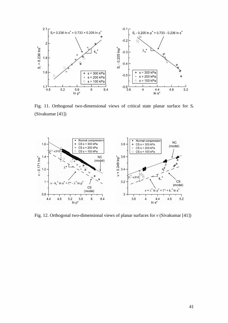
Figures 10 and 11 show pairs of orthogonal two-dimensional views of the critical state
results, presented in suitable form so that, in each view, the fitted planar surface is
reduced to a single straight line. Inspection of Figures 10 and 11 shows that the
experimental critical state results for v and Sr show a degree of scatter, but
approximate to planar surfaces in v:*ln p : *ln s and Sr:
*ln p : *ln s spaces respectively.
Tables 1 and 2 include the two sets of experimentally determined values of λ*, k1*, λs
*,
and *
2k from isotropic normal compression states and critical states respectively.
Inspection of these tables show that the two different sets of values of λ* and k1* (giving
the gradients of the planar surfaces for v) show good consistency. The values of λs* and
k2* (giving the gradients of the planar surfaces for Sr) show larger differences between
the two sets.
14
Figure 12 shows a pair of orthogonal two-dimensional representations of the isotropic
normal compression and critical state data for v . The continuous lines in Figure 12
represent the best-fit planar surface to the experimental isotropic normal compression
data, whereas the dashed lines represent the form of the critical state surface for v
predicted by the model (Equations 31 and 33), if values of * , λ* , and k1* determined
from the isotropic normal compression planar surface are employed. Inspection of the
experimental critical state values of v shows that the two planar surfaces for v are
approximately parallel, as predicted by the model, but that the vertical spacing between
the critical state and isotropic normal compression surfaces for v is significantly over-
predicted by the model. The over-prediction of the spacing between the two planar
surfaces for v is a consequence of the assumed elliptical shape of constant s* cross-
sections of the M yield surface [24] which could be adjusted following similar
developments with constitutive models for saturated soils. For example, Wheeler et al.
[50] show that incorporation of evolving plastic anisotropy in an elasto-plastic
constitutive model for saturated clays (by means of an inclined yield curve with
evolving inclination) reduces the predicted spacing between critical state line and
isotropic normal compression line in the v: pln plane.
Figure 13 shows an equivalent pair of orthogonal two-dimensional representations of
the isotropic normal compression and critical state data for Sr . Values of * , *
s and
*
2k determined from the isotropic normal compression planar surface (the solid lines)
are employed here to plot the dashed lines, which represent the form of the critical state
surface predicted by the model (Equations 32 and 34). Inspection of Figure 13 shows
that the vertical spacing between the critical state and isotropic normal compression
surfaces for Sr predicted by the model provides a reasonable match to the experimental
data, although there is significant scatter.
MODELLING TRANSITIONS BETWEEN UNSATURATED AND SATURATED
BEHAVIOUR
The GCM covers both unsaturated states (r
S < 1 ) and saturated states ( 1r
S ). For
saturated states, the GCM recovers naturally the incremental mechanical constitutive

15
relationships of the MCC model for saturated soils. This is a direct consequence of
using Bishop’s stress *
ij as a stress variable of the model because, by definition, *
ij
becomes the saturated effective stress 'ij when Sr = 1, which does not occur for the
conventional net stress variable ij unless 0s (see Equation 1).
For isotropic stress states on the M yield surface, as Sr reaches 1 the GCM response
for v should converge to the conventional saturated Normal Compression Line, NCL:
ln 'v p (35)
where λ and N are, respectively, the gradient and intercept of the saturated NCL in
the v: ln 'p plane and p′ is the saturated mean effective stress. Manipulation of
Equations 23 and 24, defining the unsaturated isotropic normal compression planar
surfaces for v and Sr , shows that for the unsaturated normal compression surface for
v (given by Equation 23) to converge to the saturated NCL (Equation 35) at Sr = 1 (as
given by Equation 24), it is necessary that κs = 0. This restriction on the value of κs is
a consequence of a small inconsistency in the GCM model highlighted by
Raveendiraraj [32], which is associated with any occurrence of plastic volumetric
strains while the soil is fully saturated (or fully dry), as illustrated in Figure 14.
Figure 14 shows a wetting stress path ABC, followed by a loading-unloading cycle
CDE (not seen in the figure) while the soil is saturated and then a drying path EFG. The
loading-unloading cycle is such that during CDE plastic volumetric strain occurs, due
to yielding on the M surface, whereas for simplicity it is assumed that no plastic
volumetric strains occur during either AB or FG, while the soil is unsaturated. As a
consequence of the plastic volumetric strain occurring while the soil is saturated,
coupled movements of the WR and DR yield surfaces occur and this means that the
water retention curves translate from the positions shown by the fine continuous lines
in Figure 14 to those shown by the fine dashed lines. As a consequence, whereas the
soil reaches a saturated state at a value of modified suction sB* during wetting, de-
saturation occurs at a higher value of modified suction sF* during subsequent drying.
This means that elastic increases of Sr occur over the range of modified suction sF*
to sB* during the wetting path (plastic changes of Sr also occur) but that elastic
decreases of Sr do not occur between sB* and sF
* during the drying path. This means

16
that elastic changes of Sr have not been reversible over the range of modified suction
sB* to sF
* , which contravenes a basic tenet of elastic behaviour.
The predicted irreversibility of elastic changes of Sr introduces inconsistency into the
model, by incorporating permanent distinction between the effects of past plastic
volumetric strains occurring at saturated states and those occurring at unsaturated states
(Raveendiraraj [32]). A simple way to overcome this problem is by assuming κs = 0,
but inevitably this may result in slight deterioration in the representation of water
retention behaviour. This sacrifice is, however, surprisingly small, because
experimental values of κs determined from tests on compacted fine-grained soils are
typically very small (e.g. [24-26]). It is therefore recommended that 0s
is assumed
when the GCM is used in situations where transitions between unsaturated and
saturated conditions occur (reducing by one the number of soil constants within the
model).
With 0s
, Figure 15 shows a three-dimensional view (in v:*ln p : *ln s space) of
both the unsaturated isotropic normal compression planar surface for v corresponding
to the intersection of M and WR yield surfaces and the saturated isotropic normal
compression line (which forms a planar surface parallel to the *ln s axis in this three-
dimensional space). The intersection of the two surfaces defines a “saturation line”
corresponding to the transition from unsaturated to saturated conditions. Figure 16
shows the equivalent surfaces for Sr (in r
S :*ln p : *ln s space), with the intersection
between unsaturated and saturated surfaces corresponding to the same saturation line
as in Figure 15. Also shown in Figures 15 and 16 is a typical stress path ASB involving
transition from unsaturated to saturated conditions at point S.
Derivation of expressions for saturation and de-saturation lines
Adopting κs = 0, Equations 21 and 22 remain unchanged, and Equations 25 and 26
become:
*
1 21
ss
k k
(36)

17
*
2 2
1 21
sk kk k
(37)
Putting Sr = 1 in Equation 24, which defines the unsaturated normal compression
planar surface for Sr , with *
s and
*
2k given by Equations 36 and 37, produces an
expression for the saturation line shown in Figures 15 and 16:
*
2*
*
* ln1
ln pkss
(38)
Inserting the expression for the saturation line of Equation 38 in the expression for the
unsaturated normal compression planar surface for v (Equation 23), gives an expression
for the saturated NCL:
1* * *1 ln
s
kv p
(39)
Comparing Equation 39 with the standard expression for the saturated NCL (Equation
35), and remembering pp * when 1
rS , shows that the intercepts
* , N* and
N are related:
*
*
1
1s
k
(40)
The saturation line defined by Equation 38 represents the combinations of *s and *p
at which transitions from unsaturated to saturated conditions will occur if the stress
state is isotropic and at the intersection between M and WR yield surfaces. With 0s
, transitions from unsaturated to saturated conditions can only occur whilst on the WR
yield surface, but it is not necessary for the stress state to be on the M yield surface or
for the stress state to be isotropic at the point of transition from unsaturated to saturated
conditions. Given that changes of *p or q do not produce elastic changes of Sr , it is
straightforward to use Equation 38 to derive a generalised expression for transition from
unsaturated to saturated conditions, applicable to any isotropic or anisotropic stress
states, including those not on the M yield surface, by considering an elastic stress path

18
along the WR yield surface from the intersection with the M yield surface at 0q . This
generalised expression for transition from unsaturated to saturated conditions under any
stress state takes the form:
*
02*
*
* ln1
ln pkss
(41)
This can be re-written as:
2*
0*
*
* 1exp
k
s
ps
(42)
The general expression for the saturation line, corresponding to transition from
unsaturated to saturated conditions (sometimes known as the air-exclusion point),
defined by Equation 41 or Equation 42, is illustrated in Figure 17 (in both a log-log plot
and a linear plot). Note that Equations 41 and 42 and Figure 17 show that the saturation
value of *s is uniquely dependent on the position of the M yield surface (i.e. the value
of *
0p ).
Transitions in the reverse direction, from saturated to unsaturated conditions, must
occur on the DR yield surface if 0s
, but it is not necessary for the stress state at the
point of de-saturation to be on the M surface. This transition from saturated to
unsaturated conditions occurs on a “de-saturation line” defined by:
2*
0*
*
* 1exp
k
s
pRs
(43)
where R is the soil constant defining the fixed ratio of *
2s to
*
1s (see Equation 15).
Figure 17 shows the form of the de-saturation line defined by Equation 43,
corresponding to transition from saturated to unsaturated conditions (sometimes known
as the air-entry point).
Figure 17 illustrates that the GCM includes the influences of both retention hysteresis
and plastic volumetric straining on transitions between saturated and unsaturated

19
conditions. The difference between the saturation and de-saturation values of *s (at
the same value of *
0p ) shows the influence of retention hysteresis, whereas the
variation of both saturation and de-saturation values of *s with *
0p shows the
influence of plastic volumetric strains on air-exclusion and air-entry points.
Mechanical yielding under saturated and unsaturated conditions
Figure 18 illustrates how the GCM provides consistent modelling of mechanical
yielding under both saturated and unsaturated conditions. The figure shows a wetting-
drying cycle ABCDEF involving transitions between unsaturated and saturated
conditions during both wetting and drying (at points B and E respectively). The stress
path starts on the WR yield surface at A but remains inside the M yield surface
throughout. The stress path shown in Figure 18 in both the *s :*p plane (Figure 18a)
and the conventional s : p plane (Figure 18b) happens to represent a wetting-drying
cycle performed at constant p , but the discussion presented in this section would
apply equally well to any general wetting-drying path remaining inside the M yield
surface.
Also shown in Figure 18a is the variation of mechanical yield stress *
0p predicted by
the GCM during the wetting-drying cycle, representing the coupled movement of the
M yield surface. The value of *
0p reduces during the initial unsaturated section AB of
the wetting path, due to the coupled inward movement of the M surface caused by the
plastic increases of Sr during yielding on the WR surface (see Equation 13). However,
during the final saturated section BC of the wetting path, the value of *
0p remains
constant, as there are no longer any plastic increases of Sr to produce further coupled
movement of the M surface. During drying path CDEF the stress path passes back inside
the WR surface at point D, but de-saturation only occurs when the stress path reaches
the DR surface at E. The value of *
0p therefore remains constant during the initial
saturated section CDE of the drying path and then increases during the final unsaturated
section EF (see Equation 13).
Figure 18b shows the variation of mechanical yield stress predicted by the GCM during
the wetting-drying cycle ABCDEF re-plotted in the conventional s : p plane. The

20
variation of mechanical yield stress during the unsaturated section AB of the wetting
path is equivalent to the LC yield curve in conventional models such as the BBM. From
B to C, however, with the soil in a saturated condition, the variation of mechanical yield
stress for the GCM plots as a 45° line in the s : p plane, consistent with yield at a
constant value of saturated mean effective stress ( spuppw
). During the
drying path CDEF the variation of mechanical yield stress follows a 45° line until the
soil de-saturates at E, and then from E to F it forms a curve again. The qualitative form
of variation of mechanical yield stress shown in Figure 18b is exactly what would be
expected for a soil under unsaturated and saturated conditions, where saturation occurs
at a non-zero air-exclusion value of suction (point B) and de-saturation occurs at a non-
zero air-entry value of suction (point E) that is higher than the air-exclusion value
because of hysteresis in the retention behaviour. This variation of mechanical yield
stress emerges naturally from the GCM, whereas it would be very difficult to achieve
in any mechanical model expressed in terms of net stresses and suction.
DETERMINATION OF MODEL PARAMETER VALUES
With 0s
, the GCM involves 10 soil constants: λ, κ, N, M, G, N*, k1, k2, s and R.
The first 5 constants are the Modified Cam Clay parameters, required for modelling of
mechanical behaviour under saturated conditions, whereas the other 5 constants are
required to extend the modelling to include mechanical behaviour under unsaturated
conditions, water retention behaviour and the coupling between them. The values of the
10 constants must be determined for a given soil if the model is to be used in numerical
simulations of single element laboratory tests or geotechnical boundary value problems
where both saturated and unsaturated conditions occur. In addition, the initial state of
the soil must be specified for any numerical simulation, including appropriate variation
of this initial state with position (e.g. with depth) in a boundary value problem.
Soil constants
The values of soil constants λ , κ and N can be determined from conventional isotropic
loading and unloading stages performed in a triaxial apparatus on saturated samples.
The value of M can be determined from experimental critical state data for saturated

21
and unsaturated samples plotted in the q :*p plane (see Equation 16), and the value
of G can be measured in triaxial shear tests on saturated or unsaturated samples (ideally
involving unload-reload stages).
It might appear that the values of soil constants s
and R would best be determined
from conventional water retention curves (measured, for example in a pressure plate
test) plotted in the r
S : *ln s plane, with s
given by the gradient of the main drying
and main wetting curves and R calculated from the spacing of the main drying curve
and the main wetting curve. However, this procedure would often give misleading
values for s
and R , because conventional water retention tests will often involve
plastic volumetric strains, and under these conditions the GCM predicts that the
gradients and spacing of the main drying and main wetting curves do not correspond
simply to s
and R. A better alternative is therefore to use experimental data from
isotropic loading under unsaturated conditions (at a minimum of two different values
of suction) to define the unsaturated isotropic normal compression planar surfaces for
v and Sr corresponding to the intersection of M and WR yield surfaces, and to use the
gradients and intercepts of these surfaces to determine the values of the soil constants
k1, k2 , s and N*.
When plotted in v :*ln p : *ln s space, the intercept of the experimental unsaturated
normal compression surface for v gives the value of the soil constant N* directly
(Equation 23). With values of and already determined from tests on saturated
samples, the two gradients * and *
1k of the experimental unsaturated normal
compression surface for v (see Equation 23) can then be used to determine values for
the soil constants k1 and k2 , by combining Equations 21 and 22 to give:
*
*
11
kk (44)
*
1
*
2k
k
(45)

22
The corresponding experimental unsaturated normal compression surface for Sr (see
Equation 24) can then be used to determine the value of the soil constant s
. With
0s
and values already determined for the soil constants , , N, N*, k1 and k2,
Equations 40, 36 and 37 show that the intercept * and the two gradients,
*
s and
*
2k
, of the unsaturated normal compression surface for Sr all depend solely on the value
of s
. Least-squares fitting of Equation 24 to the experimental data defining the planar
surface in r
S :*ln p : *ln s space, with the value of
s as the sole degree of freedom,
can be used to determine a value for s
.
The procedure described above for determining the values of N*, k1 , k2 and s
, allows
three degrees of freedom (the values of N*, k1 and k2) for fitting the intercept and the
two gradients of the unsaturated normal compression surface for v , but only a single
degree of freedom (the value of s
) for fitting the intercept and the two gradients of
the unsaturated normal compression surface for Sr. If this results in poor fitting of the
experimental data defining the unsaturated normal compression surface for Sr , it may
be appropriate to perform iterative adjustment of parameter values, to improve the fit
of the surface for Sr , whilst slightly compromising the fit of the surface for v.
The final soil constant R is required only if the GCM is to be used for simulations
involving yielding on both WR and DR retention yield surfaces. The value of R can be
determined by comparing experimental values of v for isotropic stress states at the
intersection of DR and M yield surfaces with Equation 29 (with 0s
). Suitable
experimental tests would include drying of samples starting in normally consolidated
saturated states.
The methodology for determining the values of λ, κ, N, N*, k1, k2 and s
was applied
to the experimental results of Sivakumar [41], including saturated and unsaturated tests,
resulting in the values shown in Table 3.
Initial state

23
The initial state of the soil must be specified for any numerical simulation. For the
GCM, this initial state is represented by initial values of the stress variables *
ij and
*s (*p , q and *s are sufficient for the case of a triaxial test) and initial values of the
hardening parameters *
0p and
*
1s (or
*
2s ).
For simulations of laboratory tests, it is likely that the initial state will be known in
terms of initial values of conventional stress variables, p , q and s, and initial values
of v and Sr . These can be combined to give initial values of *p , q and *s (Equations
1 and 3). With the values of soil constants already determined, the general expressions
for v and Sr of Equations 27 and 28 can be combined (using 0s
and Equations
21, 22, 36 and 37) to give expressions for the initial values of the hardening parameters
*
0p and
*
1s in terms of the initial values of
*p , v and Sr (the initial value of *s is
not involved, because of the assumption 0s
):
** *1*
0
lnln
r
s
k Sv pp
(46)
* **2*
1
lnln r
s
k v pSs
(47)
where * is given by Equation 40.
Having calculated initial values of *
0p and
*
1s from Equations 46 and 47, these should
be checked to ensure that the initial stress state does not fall outside any of the yield
surfaces. If this condition is not satisfied, it will be necessary to adjust slightly the initial
value of Sr or v (accepting that it will not then perfectly match the experimental value)
in order to adjust the values of *
0p and
*
1s (Equations 46 and 47) such that the initial
stress state now falls on or inside the relevant yield surface. Similar adjustment of the
initial value of v or Sr may be required if experimental evidence suggests that the
initial stress state lies exactly on one of the yield surfaces. To bring the initial stress
state exactly on to one of the yield surfaces, through adjustment of the initial value of
Sr or v , it will normally be necessary to employ an iterative procedure, because the
24
initial stress state is normally known in terms of the conventional stress parameters p
, q and s (rather than *p , q and *s ), and adjustment of the initial value of Sr or v
will then lead to a change of the initial value of *p or *s (see Equations 1 and 3).
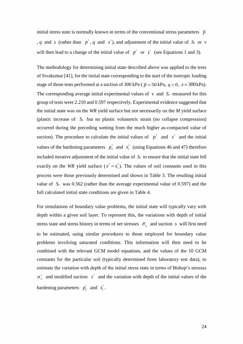
The methodology for determining initial state described above was applied to the tests
of Sivakumar [41], for the initial state corresponding to the start of the isotropic loading
stage of those tests performed at a suction of 300 kPa ( 50p kPa, 0q , 300s kPa).
The corresponding average initial experimental values of v and Sr measured for this
group of tests were 2.210 and 0.597 respectively. Experimental evidence suggested that
the initial state was on the WR yield surface but not necessarily on the M yield surface
(plastic increase of Sr but no plastic volumetric strain (no collapse compression)
occurred during the preceding wetting from the much higher as-compacted value of
suction). The procedure to calculate the initial values of *p and *s and the initial
values of the hardening parameters *
0p and
*
1s (using Equations 46 and 47) therefore
included iterative adjustment of the initial value of Sr to ensure that the initial state fell
exactly on the WR yield surface (*
1
* ss ). The values of soil constants used in this
process were those previously determined and shown in Table 3. The resulting initial
value of Sr was 0.562 (rather than the average experimental value of 0.597) and the
full calculated initial state conditions are given in Table 4.
For simulations of boundary value problems, the initial state will typically vary with
depth within a given soil layer. To represent this, the variations with depth of initial
stress state and stress history in terms of net stresses ij
and suction s will first need
to be estimated, using similar procedures to those employed for boundary value
problems involving saturated conditions. This information will then need to be
combined with the relevant GCM model equations, and the values of the 10 GCM
constants for the particular soil (typically determined from laboratory test data), to
estimate the variation with depth of the initial stress state in terms of Bishop’s stresses
*
ij and modified suction *s and the variation with depth of the initial values of the
hardening parameters *
0p and
*
1s .

25
Once the initial state of a boundary value problem has been specified, it is useful to
express the incremental mechanical and water retention relationships of the GCM, in
terms of the increments of strains and the increments of matric suction s (see [23,
24]) because, together, they define an initial value problem that can be integrated over
time at each Gauss or integration point within each finite element (i.e. local level). This
is the common procedure used in the literature for finite element analysis involving
unsaturated soils [5, 38, 43], because these two increments (i.e. , s) can be easily
approximated at the corresponding integration points, once the nodal displacements and
pore fluid pressures increments have been found from the discretized global equations.
SIMULATIONS OF EXPERIMENTAL DATA OF SIVAKUMAR (1993)
Validation of the GCM was undertaken by performing model simulations of the
experimental tests of Sivakumar [41] performed on saturated and unsaturated samples
of compacted speswhite kaolin at suctions of 0, 100, 200 and 300 kPa. Model
simulations of initial equalisation stages and isotropic loading stages are discussed here,
whereas model simulations of subsequent shearing stages are discussed elsewhere ([24,
26]). Model simulations were performed using the set of values for soil constants shown
in Table 3.
All simulations commenced from the same initial state A, corresponding to the end of
the initial equalisation stage for those samples tested at a suction of 300 kPa, as shown
in Table 4. For tests conducted at suctions of 200kPa or 100kPa the simulations
commenced with an initial wetting stage, AB or AC respectively, (at p = 50 kPa) from
300s kPa to the required value of s, to represent the remainder of the initial
equalisation stage for these tests. For tests conducted at zero suction the simulations
were designed to replicate the stress path followed by Sivakumar [41] in the initial
equalisation stage of his tests on saturated samples. This required initial isotropic
unloading AD (at 300s kPa) from 50p kPa to 40p kPa , followed by wetting
DE (at 40p kPa) from 300s kPa to 0s , and then finally isotropic unloading
EF (at 0s ) from 40p kPa to 25p kPa. These procedures ensured that
simulations performed at all four values of suction employed consistent initial states at

26
the start of the subsequent isotropic loading stages, with differences of v and Sr that
were consistent with model predictions.
Figures 19 and 20 show experimental variations of v against p* and p respectively
(with stresses on both linear and logarithmic scales) from the isotropic loading stages
performed at all four different values of suction, plotted together with the corresponding
model simulations. Variations of Sr are presented in Figure 21 against p*. In Figures 19-
21, model simulations of the initial equalisation stages from the common starting point
A are indicated by dashed lines, simulations of constant suction isotropic loading stages
are indicated by thick solid lines and experimental results for isotropic loading stages
are indicated by symbols joined by thinner solid lines.
Inspection of Figures 19 and 21 shows that the GCM simulations capture the observed
changes of v and Sr during the equalisation stages of the tests conducted at suctions
of 200kPa, 100kPa and 0, relative to the common starting point A of the simulations.
As a consequence, the predicted values of v and Sr at the start of the isotropic loading
stages of these tests (points B, C and F) show reasonable agreement with the
corresponding experimental values (predicted values of v at C and F are slightly too
high and slightly too low, respectively).
In particular, the model simulations correctly predict, at a qualitative level, the complex
pattern of swelling and collapse compression reported by Sivakumar [41] during
wetting DE to zero suction in the tests conducted on saturated samples. During the first
part of this wetting, from D to Y (see Figure 19), the soil state is on the WR yield surface
but inside the M yield surface, and elastic swelling is predicted (due to the decrease of
*p ). Coupled inward movements of the M yield surface occur, such that yield on the
M surface commences at Y, and then collapse compression is predicted from Y to S,
where the soil reaches a saturated state (at a non-zero air-exclusion value of suction).
From S to E, with the soil in a saturated condition, the model prediction shows elastic
swelling, due to the reduction of *p (where pp *
in this saturated condition), as
suction is reduced from the air-exclusion value to a final value of zero. Sivakumar [41]
observed the same qualitative pattern of behaviour in his experimental tests, with initial
wetting-induced swelling followed by wetting-induced collapse compression and then
finally more wetting-induced swelling. Conventional models expressed in terms of net

27
stresses and suction (such as the BBM) would be unable to predict the final phase of
wetting-induced swelling.
Inspection of Figure 19 shows that the GCM simulations provide an excellent match to
the experimental positions of the normal compression lines at the four different values
of suction in the v :*ln p plane. This is a consequence of selecting the values of the
model parameters , N, N*, k1 and k2 to fit the saturated isotropic NCL and the
unsaturated isotropic normal compression planar surface in v :*ln p : *ln s space. The
fact that the GCM simulations for v at the four different values of suction also match
well the experimental normal compression lines when plotted in the v : pln plane (see
Figure 20) indicates that the model has also been able to provide adequate modelling
of the variation of Sr , given that conversion of experimental and predicted values of
*p to corresponding values of p involves the experimental and predicted values of
Sr (see Equation 1).
Figure 21 shows that the GCM predictions for the variations of Sr at the three non-
zero values of suction provide a reasonable match to the experimental results, but the
match is not as good as for the corresponding variations of v (see Figure 19). This is a
consequence of allowing 3 degrees of freedom (the values of N*, k1 and k2) when
fitting the experimental data defining the unsaturated normal compression surface for
v , but only 1 degree of freedom (the value of s
) when fitting the data defining the
normal compression surface for Sr . It would have been possible to improve the fit of
the predicted variations of Sr , by adjusting some of the model parameter values, but
this would have been at the expense of slight deterioration in the fit of the predicted
values of v.
A significant conclusion arises from comparison of Figure 19b and Figure 20b: whereas
a clear pattern emerges from the experimental normal compression lines for different
values of suction when plotted in the v :*ln p plane, no such pattern is apparent when
the same experimental curves are plotted in the v : pln plane. In the v :*ln p plane
(Figure 19b), the constant suction experimental normal compression lines
corresponding to unsaturated conditions (at suctions of 100kPa, 200kPa and 300kPa)
approximate to straight parallel lines, whereas the saturated normal compression line

28
forms a straight line of lower gradient. This pattern is perfectly represented by the
GCM, which predicts that constant s isotropic normal compression lines corresponding
to unsaturated conditions approximate to straight parallel lines of gradient * in the
v :*ln p plane (the GCM would predict perfectly straight parallel lines of gradient *
if *s were held constant (see Equation 23), rather than s ), whereas the GCM predicts
a saturated isotropic normal compression line of lower gradient . In contrast, when
the same experimental curves are re-plotted in the v : pln plane (Figure 20b), the
variation of normal compression line gradient with suction appears complex and
without clear pattern. Despite this, the GCM manages to predict well the complex form
of the various normal compression lines in the v : pln plane, because the GCM is
developed in the v :*ln p plane, where the experimental results show a logical pattern,
and only then transferred to the v : pln plane. This provides a strong argument in
favour of developing models that employ mean Bishop’s stress *p as a stress state
variable, rather than mean net stress p .
Various previous authors have proposed mechanical constitutive models that involve
relatively complex relationships attempting to represent variations of a virgin
compression index with suction (Alonso et al. [1]; Wong and Mašín [52]), with degree
of saturation (Zhou and Sheng [53]) or with both s and Sr (Alonso et al. [3]). The
evidence presented in Figure 19b suggests that such complexity may be overcome by
developing models that use *p as stress state variable and fully account for the coupling
between mechanical and water retention behaviour.
CONCLUSIONS
The Glasgow Coupled Model (GCM) predicts that isotropic normal compression states
and critical states in experimental tests involving plastic volumetric strains and plastic
increases of Sr will correspond to points at the intersection of M and WR yield surfaces.
For these states, the model predicts unique unsaturated isotropic normal compression
and unsaturated critical state planar surfaces for specific volume v (in v:*ln p : *ln s
space) and also unique isotropic normal compression and critical state planar surfaces

29
for degree of saturation Sr (in Sr:*ln p : *ln s space). Experimental results from the
tests of Sivakumar [41] on unsaturated samples of compacted speswhite kaolin provide
confirmation of the existence and form of these unique unsaturated normal compression
and critical state surfaces. The GCM also provides expressions for the values of v and
Sr for any general stress states, in terms of the values of the stresses *p and *s and
the values of the hardening parameters *
0p and
*
1s .
The GCM provides consistent representation of transitions between saturated and
unsaturated states, including the influence of retention hysteresis and the effect of
plastic volumetric strains on retention behaviour. The GCM gives unique expressions
to predict saturation and de-saturation conditions (air-exclusion and air-entry points
respectively), in the form of two unique straight lines in the *ln s :*
0ln p plane. The
saturated normal compression line (NCL) plots as a planar surface in both v :*ln p :
*ln s and r
S :*ln p : *ln s spaces, and when transitions from unsaturated to saturated
conditions occur under isotropic stress states at the intersection of M and WR yield
surfaces, the saturation line corresponds to the intersection of unsaturated and saturated
isotropic normal compression planar surfaces in both spaces.
The GCM provides consistent modelling of mechanical behaviour across the transitions
between saturated and unsaturated conditions, including appropriate representation of
the variation of mechanical yield stress. This appropriate variation of mechanical yield
stress across transitions between unsaturated and saturated conditions occurring at non-
zero values of suction emerges naturally from the GCM, whereas it would be very
difficult to achieve in any mechanical model expressed in terms of net stresses and
suction.
A straightforward methodology is proposed (and has been demonstrated) for
determining the values of all GCM model parameters and initial state from a limited
number of suction-controlled triaxial tests. Central to this methodology is plotting the
experimental data defining the unsaturated isotropic normal compression planar
surfaces in v :*ln p : *ln s and
rS :
*ln p : *ln s spaces.

30
GCM simulations of the isotropic loading stages of the experimental tests of Sivakumar
[41] on compacted speswhite kaolin demonstrate that the model is able to predict
accurately the variations of both v and Sr during isotropic stress paths under saturated
and unsaturated conditions. A clear pattern emerges when the experimental results for
unsaturated and saturated isotropic normal compression states are plotted against *ln p
, whereas no such pattern is apparent when the same results are plotted against pln .
The GCM represents the clear pattern observed in the v :*ln p plane and, as a
consequence, also captures the complex variation of the experimental results when re-
plotted in the v : pln plane. This would be extremely difficult to achieve with any
constitutive model developed in terms of net stresses and suction, and this provides a
strong argument in favour of models, such as the GCM, which employ *p as a stress
state variable.
ACKNOWLEDGEMENTS
The first author acknowledges the financial support by the Synergy Postgraduate
Scholarships scheme and the Australian Research Council Centre of Excellence in
Geotechnical Science and Engineering (CGSE).
REFERENCES
1. Alonso EE, Gens A, Josa A (1990) A constitutive model for partially saturated
soils. Géotechnique 40(3):405–430
2. Alonso EE, Olivella S, Pinyol NM (2005) A review of Beliche Dam.
Géotechnique 55(4):267–285
3. Alonso EE, Pinyol NM, Gens A (2013) Compacted soil behaviour: initial state,
structure and constitutive modelling. Géotechnique 63(6):463–478
4. Bishop AW (1959) The principle of effective stress. Tek. Ukeblad 39, 859–863
5. Borja RI (2004) Cam-Clay plasticity, Part V: A mathematical framework for
three-phase deformation and strain localization analyses of partially saturated porous
media. Comput Methods Appl Mech Eng 193: 5301–5338
6. Borja RI, White JA (2010) Continuum deformation and stability analyses of a
steep hillside slope under rainfall infiltration. Acta Geotech 5:1–14
31
7. Borja RI, Liu X, White JA (2012) Multiphysics hillslope processes triggering
landslides. Acta Geotech 7:261–269
8. Burton GJ, Sheng D, Airey D (2014) Experimental study on volumetric
behaviour of Maryland clay and the role of degree of saturation. Can Geotech J
51:1449–1455
9. Buscarnera G, Nova R (2009) An elasto-plastic strain hardening model for soil
allowing for hydraulic bonding debonding effects. Int J Numer Anal Meth Geomech
33:1055–1086
10. Casini F (2008) Effetti del grado di saturazione sul comportamento meccanico
di un limo. PhD Thesis, Universitá degli Studi di Roma ‘‘La Sapienza’’
11. Casini F, Serri V, Springman SM (2013) Hydromechanical behaviour of a silty
sand from a steep slope triggered by artificial rainfall: from unsaturated to saturated
conditions. Can Geotech J 50:28–40
12. Della Vecchia G, Romero E, Jommi C (2013) A fully coupled elastic–plastic
hydromechanical model for compacted soils accounting for clay activity. Int J Numer
Anal Meth Geomech 37:503–535
13. D'Onza F, Gallipoli D, Wheeler SJ, Casini F, Vaunat J, Khalili N, Laloui L,
Mancuso C, Mašín D, et al. (2011) Benchmark of constitutive models for unsaturated
soils. Géotechnique 61(4): 283–302
14. D'Onza F, Wheeler SJ, Gallipoli D, Barrera M, Hofmann M, Lloret-Cabot M,
Lloret A, Mancuso C, Pereira J-M et al. (2015) Benchmarking selection of parameter
values for the Barcelona basic model. Engineering Geology 196:99–118
15. Gallipoli D, Wheeler SJ, Karstunen M (2003) Modelling the variation of degree
of saturation in a deformable unsaturated soil. Géotechnique 53(1):105–112
16. Gallipoli D, Gens A, Chen G, D'Onza F (2008) Modelling unsaturated soil
behaviour during normal consolidation and at critical state. Comp Geotech 35(6):825–
834
17. Gens A (2010) Soil–environment interactions in geotechnical engineering.
Géotechnique 60(1):3–74
18. Houlsby GT (1997) The work input to an unsaturated granular material.
Géotechnique 47(1):193–196
19. Jommi C (2000) Remarks on the constitutive modelling of unsaturated soils. In:
Tarantino A, Mancuso C (ed) Experimental evidence and theoretical approaches in
unsaturated soils. Rotterdam: Balkema, pp 139-153

32
20. Josa A (1988) Un modelo elastoplastico para suelos no saturados. PhD Thesis,
Universitat Politècnica de Catalunya
21. Khalili N, Habte MA, Zargarbashi S (2008) A fully coupled flow deformation
model for cyclic analysis of unsaturated soils including hydraulic and mechanical
hysteresis. Comp Geotech 35(6):872–889
22. Laloui L, Ferrari A, Li C, Eichenberger J (2016) Hydro-mechanical analysis of
volcanic ash slopes during rainfall. Géotechnique 66(3):220–231
23. Lloret M. (2011) Numerical modelling of coupled behaviour in unsaturated
soils. PhD Thesis, University of Strathclyde and University of Glasgow
24. Lloret-Cabot M, Sánchez M, Wheeler SJ (2013) Formulation of a three-
dimensional constitutive model for unsaturated soils incorporating mechanical-water
retention couplings. Int J Numer Anal Methods Geomech 37:3008–3035
25. Lloret-Cabot M, Wheeler SJ, Sánchez M (2014) Unification of plastic
compression in a coupled mechanical and water retention model for unsaturated soils.
Can Geotech J 51(12):1488–1493
26. Lloret-Cabot M, Wheeler SJ, Pineda JA, Sheng D, Gens A (2014). Relative
performance of two unsaturated soil models using different constitutive variables. Can
Geotech J 51(12):1423–1437
27. Mašín D (2010) Predicting the dependency of a degree of saturation on void
ratio and suction using effective stress principle for unsaturated soils. Int J Numer Anal
Methods Geomech 34:73–90
28. Monroy R (2006) The influence of load and suction changes on the volumetric
behaviour of compacted London Clay. PhD Thesis, Imperial College
29. Monroy R, Zdravkovic L, Ridley A (2008) Volumetric behaviour of compacted
London Clay during wetting and loading. In: Toll DG, Augarde CE, Gallipoli D,
Wheeler SJ (ed) Proc. 1st Eur. Conf. Unsaturated Soils, Durham, pp 315–320
30. Monroy R, Zdravkovic L, Ridley A (2010) Evolution of microstructure in
compacted London Clay during wetting and loading. Géotechnique 60(2):105–119
31. Nuth M, Laloui L (2008) Advances in modelling hysteretic water retention
curve in deformable soils. Comp Geotech 35(6):835–844
32. Raveendiraraj A (2009) Coupling of mechanical behaviour and water retention
behaviour in unsaturated soils. PhD Thesis, University of Glasgow
33
33. Romero E (1999) Characterisation and thermo-hydro-mechanical behaviour of
unsaturated Boom clay: an experimental study. PhD Thesis, Universitat Politècnica de
Catalunya
34. Romero E, Della Vecchia G, Jommi C (2011) An insight into the water retention
properties of compacted clayey soils. Géotechnique 61(4):313–328
35. Roscoe KH, Burland JB (1968) On the generalised stress-strain behavior of
‘wet’ clay. In: Heyman J Leckie FA (ed) Engineering Plasticity, Cambridge University
Press, pp 535–609
36. Schrefler BA (1984) The finite element method in soil consolidation (with
applications to surface subsidence). PhD Thesis, University College of Swansea
37. Sharma RS (1998) Mechanical behaviour of unsaturated highly expansive clays.
PhD Thesis, University of Oxford
38. Sheng D (2011) Review of fundamental principles in modelling unsaturated soil
behaviour. Comp Geotech 38: 757–776
39. Sheng D, Fredlund DG, Gens A (2008) A new modelling approach for
unsaturated soils using independent stress variables. Can Geotech J 45:511–534
40. Sheng D, Zhou A (2011) Coupling hydraulic with mechanical models for
unsaturated Soils. Can Geotech J 48:826–840
41. Sivakumar V (1993) A critical state framework for unsaturated soil. PhD
Thesis, University of Sheffield
42. Sivakumar V, Wheeler SJ (2000) Influence of compaction procedure on the
mechanical behaviour of an unsaturated compacted clay, Part 1: Wetting and isotropic
compression. Géotechnique 50(4):359–368
43. Song X, Borja RI (2014) Mathematical framework for unsaturated flow in the
finite deformation range. Int J Numer Meth Eng 14:658–682
44. Sun DA, Sheng D, Xu Y (2007) Collapse behaviour of unsaturated compacted
soil with different initial densities. Can Geotech J. 44:673–686
45. Tarantino A, De Col E (2008) Compaction behaviour of clay. Géotechnique
58(3):199–213
46. Tarantino A (2009) A water retention model for deformable soils. Géotechnique
59(9):751–762
47. Tarantino A, Tombolato S (2005) Coupling of hydraulic and mechanical
behaviour in unsaturated compacted clay. Géotechnique 55(4):307–317

34
48. Vaunat J, Romero E, Jommi C (2000) An elastoplastic hydro-mechanical model
for unsaturated soils. In: Tarantino A, Mancuso C (ed) Experimental evidence and
theoretical approaches in unsaturated soils. Rotterdam: Balkema, pp 121–138
49. Wheeler SJ, Sivakumar V (1995) An elasto-plastic critical state framework for
unsaturated soil. Géotechnique 45(1):35–53
50. Wheeler SJ, Näätänen A, Karstunen M, Lojander M (2003) An anisotropic
elastoplastic model for soft clays. Can Geotech J 40:403–418
51. Wheeler SJ, Sharma RS, Buisson MSR (2003) Coupling of hydraulic hysteresis
and stress–strain behaviour in unsaturated soils. Géotechnique 53(1):41–54
52. Wong KS, Mašín D (2014) Coupled hydro-mechanical model for partially
saturated soils predicting small strain stiffness. Comp Geotech 61:355–369
53. Zhou A, Sheng D (2015) An advanced hydro-mechanical constitutive model for
unsaturated soils with different initial densities. Comp Geotech 63:46–66
35
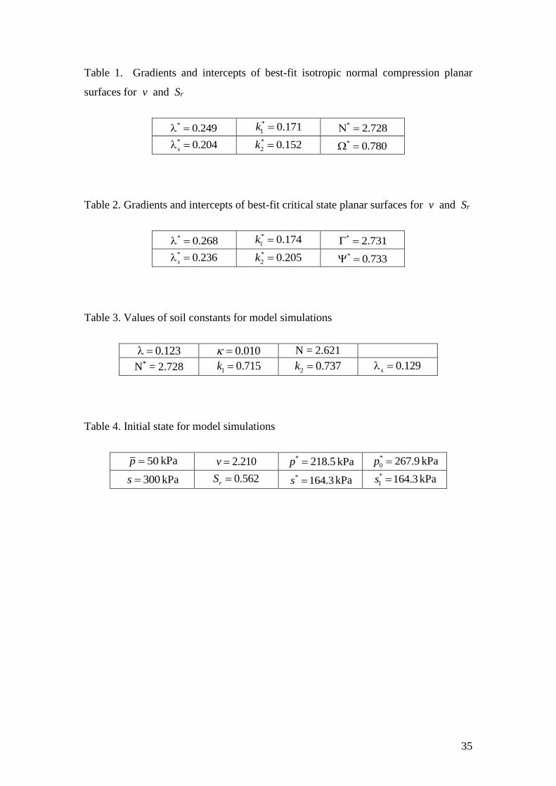
Table 1. Gradients and intercepts of best-fit isotropic normal compression planar
surfaces for v and Sr
* 0.249 *
1 0.171k * 2.728 * 0.204s *
2 0.152k * 0.780
Table 2. Gradients and intercepts of best-fit critical state planar surfaces for v and Sr
* 0.268 *
1 0.174k * 2.731 * 0.236s *
2 0.205k * 0.733
Table 3. Values of soil constants for model simulations
0.123 010.0 N = 2.621
N* = 2.728 1 0.715k 2 0.737k 0.129s
Table 4. Initial state for model simulations
50p kPa 210.2v * 218.5p kPa *
0 267.9p kPa
300s kPa 0.562rS 3.164* s kPa *
1 164.3s kPa

36
Fig. 1. Yield surfaces in Glasgow Coupled Model (GCM)
Fig. 2. Modelling retention behaviour and treatment of saturated conditions

37
Fig. 3. Positions of various points relative to the yield surfaces
Fig. 4. Isotropic normal compression planar surface for v (Sivakumar [41])

38
Fig. 5. Isotropic normal compression planar surface for Sr (Sivakumar [41])
Fig. 6. Orthogonal two-dimensional views of isotropic normal compression planar
surface for v (Sivakumar [41])

39
Fig. 7. Orthogonal two-dimensional views of isotropic normal compression planar
surface for Sr (Sivakumar [41])
Fig. 8. Critical state planar surface for v (Sivakumar [41])
40
Fig. 9. Critical state planar surface for Sr (Sivakumar [41])
Fig. 10. Orthogonal two-dimensional views of critical state planar surface for v
(Sivakumar [41])
41
Fig. 11. Orthogonal two-dimensional views of critical state planar surface for Sr
(Sivakumar [41])
Fig. 12. Orthogonal two-dimensional views of planar surfaces for v (Sivakumar [41])

42
Fig. 13. Orthogonal two-dimensional views of planar surfaces for Sr (Sivakumar [41])
Fig. 14. Demonstration of irreversible elastic changes of Sr if s > 0

43
Fig. 15. Isotropic normal compression planar surfaces for v for unsaturated and
saturated conditions
Fig. 16. Isotropic normal compression planar surfaces for Sr for unsaturated and
saturated conditions

44
Fig. 17. Predicted saturation and de-saturation lines
Fig. 18. Variation of mechanical yield stress during a wetting-drying cycle

45
Fig. 19. Model predictions and experimental variations of v against p* (Sivakumar
[41]): (a) Linear scale; (b) Logarithmic scale

46
Fig. 20. Model predictions and experimental variations of v against p (Sivakumar
[41]): (a) Linear scale; (b) Logarithmic scale

47
Fig. 21. Model predictions and experimental variations of Sr against p* (Sivakumar
[41]): (a) Linear scale; (b) Logarithmic scale

48
Fig. 1. Yield surfaces in Glasgow Coupled Model (GCM)
Fig. 2. Modelling retention behaviour and treatment of saturated conditions
Fig. 3. Positions of various points relative to the yield surfaces
Fig. 4. Isotropic normal compression planar surface for v (Sivakumar [41])
Fig. 5. Isotropic normal compression planar surface for Sr (Sivakumar [41])
Fig. 6. Orthogonal two-dimensional views of isotropic normal compression planar
surface for v (Sivakumar [41])
Fig. 7. Orthogonal two-dimensional views of isotropic normal compression planar
surface for Sr (Sivakumar [41])
Fig. 8. Critical state planar surface for v (Sivakumar [41])
Fig. 9. Critical state planar surface for Sr (Sivakumar [41])
Fig. 10. Orthogonal two-dimensional views of critical state planar surface for v
(Sivakumar [41])
Fig. 11. Orthogonal two-dimensional views of critical state planar surface for Sr
(Sivakumar [41])
Fig. 12. Orthogonal two-dimensional views of planar surfaces for v (Sivakumar [41])
Fig. 13. Orthogonal two-dimensional views of planar surfaces for Sr (Sivakumar [41])
Fig. 14. Demonstration of irreversible elastic changes of Sr if κs > 0
Fig. 15. Isotropic normal compression planar surfaces for v for unsaturated and
saturated conditions
Fig. 16. Isotropic normal compression planar surfaces for Sr for unsaturated and
saturated conditions
Fig. 17. Predicted saturation and de-saturation lines

49
Fig. 18. Variation of mechanical yield stress during a wetting-drying cycle
Fig. 19. Model predictions and experimental variations of v against p* (Sivakumar
[41]): (a) Linear scale; (b) Logarithmic scale
Fig. 20. Model predictions and experimental variations of v against p (Sivakumar
[41]): (a) Linear scale; (b) Logarithmic scale
Fig. 21. Model predictions and experimental variations of Sr against p* (Sivakumar
[41]): (a) Linear scale; (b) Logarithmic scale