Literature Review of State of the Art Numerical and Analytical Approaches to Problems in

Spine Mechanics

MAE 586: Project Work in Mechanical Engineering

Modeling of the Human Spine

North Carolina State University

Raleigh, North Carolina

May 2016

Prepared by:

Christine Reubi

Advisor:

Dr. Andre Mazzoleni

i

Table of Contents

1. Introduction ........................................................................................................................... 1

2. Background ............................................................................................................................ 1

2.1 Biological Structures ...................................................................................................... 2

2.1.1 Vertebrae ................................................................................................................. 2

2.1.2 Intervertebral Discs ................................................................................................ 5

2.1.3 Ligaments................................................................................................................. 6

2.2 Interbody Devices ........................................................................................................... 8

3. State of the Art Numerical and Analytical Approaches .................................................... 9

3.1 Disc Mechanics ............................................................................................................... 9

3.1.1 Analytical Model of Intervertebral Disc Mechanics .......................................... 10

3.1.2 Viscoelastic Numerical Model of Intervertebral Disc Mechanics .................... 14

3.2 Ligament Models ......................................................................................................... 21

3.3 Multiscale Optimization .............................................................................................. 22

3.4 Artificial Neural Networks .......................................................................................... 25

4. Discussion ............................................................................................................................. 27

4.1 Model Limitations ........................................................................................................ 28

4.1.1 Disc Model Limitations......................................................................................... 28

4.1.2 Multiscale Optimization Limitations .................................................................. 29

4.2 Future Analysis Opportunities .................................................................................... 30

4.2.1 Disc Analysis .......................................................................................................... 30

4.2.2 Interbody Device Design....................................................................................... 31

4.3 Summary ....................................................................................................................... 31

References .................................................................................................................................... 33

ii

List of Figures

Figure 1: Vertebral Body (A) Side View and (B) Top View ..................................................... 3

Figure 2: Internal Trabeculae Structure of the Vertebral Body .............................................. 3

Figure 3: Left Lateral View of the Vertebral Body with Posterior Elements ......................... 4

Figure 4: Simplified Model of the Lumbar Spine ...................................................................... 4

Figure 5: Structure of an Intervertebral Disc ............................................................................ 5

Figure 6: Compressive Stress Applied to an Intervertebral Disc ............................................. 6

Figure 7: Section of the Lumbar Spine Including Ligaments................................................... 7

Figure 8: Schematic Diagram of the Intervertebral Disc ........................................................ 10

Figure 9: Diagram of the Fiber Angle and Membrane Stress Resultants ............................. 11

Figure 10: Diagram of the Equilibrium State of the Membrane ............................................ 12

Figure 11: Spring and Dashpot Diagram of the Zener Model ................................................ 15

Figure 12: Network Diagram of the Viscoelastic Model ......................................................... 16

Figure 13: Influence of Parameter τ for c1e = 0 and ɳ = 1 ....................................................... 17

Figure 14: Influence of Parameter τe for c1 = 0 and ɳ = 1 ....................................................... 18

Figure 15: Influence of Parameter ɳ for c1 and c1e = 1 ............................................................ 18

Figure 16: Pressure Distribution within the Intervertebral Disc ........................................... 20

Figure 17: von Mises Stress Distribution within the Intervertebral Disc .............................. 20

Figure 18: AF NP Relative Contributions to the Intervertebral Disc Resultant Force........ 21

Figure 19: Geometrical Model (C2-T1) .................................................................................... 22

Figure 20: Finite Element Model (C2-T1) ................................................................................ 23

Figure 21: Design Process for ALIF Cage Design.................................................................... 25

Figure 22: Artificial Neural Network Process Diagram .......................................................... 27

List of Tables

Table 1: Boundary and Load Conditions for Analytical Disc Model .................................... 12

Table 2: Intervertebral Disc Dimensions for 2-D Axisymmetric COMSOL Model ............. 19

Table 3: Material Constants for COMSOL Simulation .......................................................... 20

Table 4: COMSOL Simulation Parameters for the Nucleus Pulposus .................................. 21

Table 5: FEA Input Parameters ................................................................................................ 26

Table 6: Final Result of ANN Analysis ..................................................................................... 27

Page 1 of 34

1. Introduction

In order to inform future analytical and numerical studies for problems in spine

mechanics, this literature review presents a collection of state of the art analyses and

discusses the limitations of each. This investigation describes analyses of

intervertebral disc mechanics and of interbody fusion device design. These analyses

involve simplifying assumptions and generally utilize data from healthy spines as

validation for the results. Future analyses look to improve researchers’ and

physicians’ understanding of the behavior of diseased or damaged human spinal

structures.

The effects of scoliosis and the efficacy of fusion as a treatment are of particular

interest to the study of spine mechanics and to interbody fusion device research and

development. Scoliosis involves a structural deformation of the spine that may occur

in any region of the vertebral column, though more prevalent in the thoracic and

lumbar regions. This spinal deformation indicative of this disease affects the

surrounding tissues and, critically, the intervertebral discs. The deformation alters

stress distributions within the disc; however, the current state of the art in disc

mechanics has thus far focused on the simplifying assumptions of a uniform load

applied to an axisymmetric disc structure. Further study and experimentation of the

disc response may provide additional insight into why and how intervertebral discs

degenerate and fail in scoliotic patients so that treatment may be developed.

Diseases such as scoliosis and spondylolisthesis may require interbody fusion as a

treatment to prevent further progression of the disease by limiting movement of the

spinal column. Interbody fusion cages use bone grafts to fuse adjacent vertebrae and

are frequently applied to the lumbar region of the spine with the goal of reducing pain

in the patient’s back. This review includes two state of the art design methods for

developing highly effective interbody fusion cages. The studies summarized herein

introduce a multiscale optimization technique to optimize the effectiveness of

vertebral fusion and to employ an artificial neural network analysis to reduce the

occurrence of fusion failure.

2. Background

To fully understand the anatomy required to study problems in spine mechanics,

some background is provided on the biological structures within the spine. The

different sections of vertebral columns within the spine (cervical, thoracic, and

lumbar) through the sacrum are described in the sections that follow, as well as the

associated intervertebral discs and ligaments. Following the biological background of

the spine, a brief overview of interbody fusion devices is given. Design of these

devices and analysis of their effects on the surrounding structure are perhaps the most

crucial applications dealing with biomechanics of the spine.

Page 2 of 34

2.1 Biological Structures

The cervical spine resides at the top of the spinal column. This section features

small vertebral bodies, and cervical disc height is thick compared to the scale of

the cervical vertebrae. These large discs allow the cervical spine greater mobility,

which can be experienced by extending, flexing, or rotating the head. From top

to bottom, the cervical vertebrae are numbered C1-C7. Intervertebral discs are

named by the vertebrae they reside between. The cervical spine contains the C1-

C2, C2-C3, C3-C4, C4-C5, C6-C7, and C7-T1 discs [1]. The analyses discussed

here will not generally deal with analysis of the cervical spine but with that of

the lumbar spine.

Below the cervical spine, sits the thoracic spine, which includes the thoracic

vertebrae and discs, the ribs, and the sternum. This section transfers compressive

loads to the lumbar spine below [1]. Thoracic vertebrae number from T1 to T12,

and the corresponding discs are named as T1-T2 through T12-L1.

Most of the analysis review and discussion will focus on the lumbar spine. The

lumbar column contains five vertebral elements, L1-L5. The associated lumbar

discs are named L1-L2 through L4-L5. An additional intervertebral disc, the

lumbosacral disc, separates the L5 from the sacrum, L5-S1. Some analyses also

include the sacrum, which supports the lumbar column. This bone transmits

loads from the spine to the lower limbs [1].

The spine allows movement between the skull and the pelvis through four basic

motions: flexion, extension, lateral bending, and axial rotation. Flexion occurs

when the torso curves forward into a bend. Extension bends the spine back from

a standing posture into an arch, which is opposite from flexion. Lateral bends

bend the spine from side to side (i.e., left or right). Finally, axial rotation is a

twist around the plane of the spinal column. These movements indicate the types

of loads that are applied in detailed analysis.

2.1.1 Vertebrae

The vertebral components of the human spine sustain compressive loads

that are transmitted from the trunk onto the spine. To support these

compressive loads, each vertebrae contains two types of bone: cortical and

trabecular. The cortical bone serves as the outer shell of the roughly

cylindrical vertebral body (Figure 1). Overlapping vertical and horizontal

trabeculae reinforce the structure of the vertebral body by adding support

to carry compressive loads and to prevent buckling. The reinforcing effect

of the trabeculae is demonstrated in Figure 2 and described in greater

detail in The Biomechanics of Back Pain [1].

Page 3 of 34

Figure 1: Vertebral Body (A) Side View and (B) Top View [1]

Figure 2: Internal Trabeculae Structure of the Vertebral Body [1]

Without posterior elements, the vertebral bodies would slide front to back

or side to side along the spinal column. Posterior elements (Figure 3)

constrain the movement of each vertebrae. These additional bone

structures also provide attachment sites for muscles along the spinal

column. These muscles apply loads to bend or twist the spine indirectly by

leveraging the posterior elements [1].

Page 4 of 34

Figure 3: Left Lateral View of the Vertebral Body with Posterior Elements (VB =

Vertebral Body, P = Pedicle, TP = Transverse Process, iaf = Inferior Articular Facet,

SP = Spinous Process) [1]

Understanding the vertebrae and their structure sets the stage for the

analysis environments discussed in this review. Vertebrae are often key

modeling components in finite element and other numerical analyses.

Typically, actual patient computed tomography (CT) scans form the basis

of these models and provide incredible detail. More simplified models

(Figure 4), such as proposed by Xiaoyang Wang, save computing time

while still providing insightful results [2].

Figure 4: Simplified Model of the Lumbar Spine [2]

Page 5 of 34

2.1.2 Intervertebral Discs

Between each consecutive vertebra in the spine, an intervertebral disc

evenly transmits the compressive load while enabling bending movement

in the torso. The summation of all intervertebral discs contributes about

25% of the total spine length [1]. These discs have a structure consisting

of three components – a central gel known as the nucleus pulposus (NP),

sheets of tightly packed lamellae that comprise the annulus fibrosus (AF),

and vertebral end plates (VEP) that sandwich the disc on top and bottom

Figure 5). All three components are essential for stable, supportive discs.

The nucleus pulposus is

a gel-like material

located at the center of

each intervertebral disc

that expands under

compressive loading.

This gel consists of

proteoglycans,

composed of complex

sugars and protein.

These proteoglycans

retain water essential for

healthy disc function.

Within the center of the

disc, the nucleus

pulposus acts as a fluid

with a hydrostatic

pressure; however,

under rapid loading, it

behaves as a viscoelastic

solid [1]. For the

purposes of disc

modeling, it is critical to

understand these fluid

mechanical properties

and behavior of the

nucleus pulposus.

The nucleus pulposus prevents the annulus fibrosus from buckling under

compression by expanding and generating hoop stress within the wall of

the annulus fibrosus (Figure 6). 10-20 sheets of collagen lamellae form

this wall to sustain the compressive loads of the spine. In each sheet,

Figure 5: Structure of an Intervertebral Disc (VEP =

Vertebral End Plate, NP = Nucleus Pulposus, AF =

Annulus Fibrosus) [1]

Page 6 of 34

collagen fibers are oriented at an angle of approximately 65o. The sheets

are successively ordered in opposing orientations to maintain the integrity

of the disc wall. Fibers in the annulus fibrosus curve from endplate to

endplate, which may cause more complex geometrical modeling problems.

These fibers sustain tensile stress produced by the aforementioned

expansion of the nucleus pulposus that is of keen interest for spine

mechanics [1].

Figure 6: Compressive Stress Applied to an Intervertebral Disc Generates Tensile

Hoop Stress in the Annulus Fibrosus [1]

Inner fibers of the annulus fibrosus attach directly into the vertebral

endplates that bind the disc to the vertebrae. The superior endplate resides

at the top of the intervertebral disc; while, the inferior endplate bonds to

the bottom of the disc structure (Figure 5). Endplates are composed of

cartilage that is loosely bonded to the bone and supported by the

hydrostatic pressure provided by the nucleus pulposus [1].

2.1.3 Ligaments

Upon review of a number of studies for interbody cage design using finite

element methods, certain ligaments of the spine are frequently considered

in analysis:

Page 7 of 34

Figure 7: Section of the Lumbar Spine Including Ligaments (ALL = Anterior

Longitudinal Ligament, PLL = Posterior Longitudinal Ligament, SSL = Supraspinous

Ligament, ISL = Interspinous Ligament, v = Ventral Part, m = Middle Part, d = Dorsal

Part, LF = Ligamentum Flavum) [1]

Interspinous and Supraspinous

The interspinous ligament (ISL) connect the edges of the spinous

processes on the posterior elements of the vertebrae with sheets of

collagen fiber. Supraspinous ligaments (SSL) are actually tendinous fibers

that attach to muscles in the back. These ligaments may be entirely absent

from the lower spine beyond the L3 vertebra. Both the interspinous and

supraspinous ligaments merge together. Their fibers are intertwined,

which significantly increases the combined tensile stiffness of the

ligament structure [1]. This consideration may be key to accurately

modeling any influence of these ligaments on the spine.

Page 8 of 34

Intertransverse

Residing between the transverse processes of the posterior vertebrae

elements, the intertransverse ligament consists of collagen membranes that

separate the ventral muscle compartment from the dorsal muscle

compartment. This ligament stretches most significantly of all the

ligaments of the spine and plays a key role in the action of bending [1].

Ligamentum Flavum

As shown in Figure 7, the ligamentum flavum connects the internal

surface of one posterior lamina of the vertebrae to the external surface of

the one below. This ligament is composed of elastin fibers that stretch and

extend during flexion [1].

Capsular

Situated laterally to the mid-sagittal plane, capsular ligaments resist

bending movement in any direction [1].

Posterior Longitudinal

According to The Biomechanics of Back Pain, “the posterior longitudinal

ligament covers the floor of the vertebral canal,” as shown in Figure 7.

This ligament attaches to the posterior elements and the intervertebral

discs [1].

Anterior Longitudinal

Similar to the posterior longitudinal ligament, the anterior longitudinal

ligament connects to the intervertebral discs and to the anterior edges of

the vertebrae (Figure 7). This ligament is stronger and thicker than its

posterior counterpart [1].

2.2 Interbody Devices

Interbody cages fuse segments of the spine together to reduce back pain for those

patients suffering disc degeneration. According to The Biomechanics of Back

Pain, “Their aim is to restore height, lordosis and sagittal balance, while placing

the remaining annular fibers under tension” [1]. These devices also limit motion

in the fused segment of the spine, which is a key concern in interbody cage

design and analysis.

Page 9 of 34

Types of Interbody Fusion

Analyses and designs for interbody fusion devices often reflect the type of lumbar

interbody fusion surgery that will be used to implement the device. There are

three main categories of lumbar interbody fusion procedures – anterior, posterior,

and transforaminal. Anterior lumbar interbody fusion (ALIF) is performed

through the front of the body and most commonly involves removal of an

intervertebral disc and implantation of a device and bone graft. For diseases such

as scoliosis or spondylolisthesis, posterior lumbar interbody fusion (PLIF) is

utilized. A disc is also removed and an interbody device is implanted with a bone

graft, similar to the procedure for ALIF. Transforaminal lumbar interbody fusion

(TLIF) works on both the anterior and posterior simultaneously [3]. Interbody

fusion also has applications to the cervical and thoracic spine using similar

methods and similar fusion devices, though the scale of these devices differs from

that of the lumbar fusion cages.

Materials for Cage Devices

Interbody cage devices for spinal fusion are manufactured from a variety of

materials. Most commonly used materials include titanium, polyetheretherketone

(PEEK), composites (carbon-fiber reinforced), and bioabsorbable polymers (poly-

L, D-lactic acid (PLDLA)). Though titanium provides significantly large load

bearing capability and strength, its material properties are also much greater than

those of the surrounding bone and tissue components of the spine. These titanium

cages also interfere with radiographic techniques and apply abnormal load

distributions on the vertebral endplates [1]. Materials that display properties

closer to that of the surrounding structure may have clinical benefits over

titanium. In the discussion of design analyses (sections 3.3 and 3.4), the most

commonly used materials are titanium and PEEK; however, section 3.3 attempts

to optimize the properties of a biomaterial for enhancing vertebral fusion.

3. State of the Art Numerical and Analytical Approaches

Understanding the state of the art in numerical and analytical approaches to a variety

of problems in spine mechanics gives insight into the historical foundation of research

and experimentation. This review also helps form future analysis by identifying

limitations in technology or resources, such as time. In this literature review, two

analyses of disc mechanics and two methods for designing interbody fusion cages are

summarized.

3.1 Disc Mechanics

Analysis of intervertebral disc mechanics provides researchers and doctors with a

view of how discs fail and lead to disc replacement or surgical stabilization.

Researchers can also begin to understand how the disc behaves in bending, how

Page 10 of 34

the viscoelastic nucleus pulposus affects disc stress response and failure, and

why certain conditions of the spine increase the risk for disc degeneration and

failure. The following sections provide overviews of the development of an

analytical model of disc mechanics that assumes a uniformly applied

compressive load and an attempt to numerically describe the viscoelastic

behavior of the disc under rapid loading.

3.1.1 Analytical Model of Intervertebral Disc Mechanics

Very few recent studies exist that probe into analytical modeling of the

intervertebral disc structures to determine their mechanical response. One

often cited model by McNally and Arridge [4] examines the mechanical

response of an axisymmetric, thin-walled disc structure under a uniformly

applied load. To develop analytical models of the intervertebral disc, the

geometry is simplified, allowing the disc to be modeled as a whole with

fewer boundary conditions and assumptions than for a numerical model.

This model improves on previous work by allowing the equilibrium

equations to determine the shape the annulus fibers take under load

conditions, rather than prescribing an arbitrary shape.

Figure 8: Schematic Diagram of the Intervertebral Disc in the Coordinate System [4]

A geometrical diagram of the model is displayed by Figure 8. The disc is

axisymmetric with circular symmetry about the z-axis. rθ and rΦ represent

the two radii of curvature for the disc membrane. In this model, the

membrane is the simplified depiction of the annulus fibrosus. By

considering the hydrostatic pressure (p) applied to the membrane by the

central nucleus pulposus, as discussed in section 2.1.2, the components of

the membrane stress (Nθ and NΦ) are in equilibrium:

Page 11 of 34

𝑁𝜃

𝑟𝜃+

𝑁𝜙

𝑟𝜙= 𝑝

Figure 9: Diagram of the Fiber Angle and Membrane Stress Resultants [4]

Figure 9 shows the cross-hatched pattern the alternating layers of the

annulus fibrosus create. The collagen fibers are oriented at an angle β,

which is described in section 2.1.2 as typically an angle of 65o. This

analysis utilizes two different, separate treatments of the collagen fibers.

The first, the trellis rule, states that “the fibres in any one layer are

considered as frictionlessly ‘pin-jointed’ to those in the layer beneath so

that the layers then deform like a piece of trellis [4].”

tan2𝛽

𝑟=

𝑟 sin2 𝛽𝑐

𝑟𝑐2 − 𝑟2 sin2 𝛽𝑐

𝑟𝑐 = 𝑟𝑎𝑑𝑖𝑢𝑠 𝑎𝑡 𝑡ℎ𝑒 𝑒𝑞𝑢𝑎𝑡𝑜𝑟𝑖𝑎𝑙 𝑝𝑙𝑎𝑛𝑒

𝛽𝑐 = 𝛽 𝑎𝑡 𝑡ℎ𝑒 𝑒𝑞𝑢𝑎𝑡𝑜𝑟𝑖𝑎𝑙 𝑝𝑙𝑎𝑛𝑒 (𝑧 = 0, 𝑟 = 𝑟𝑐)

A second treatment of the fibers is performed using the geodesic law.

“Fibres, which are independent of each other, are assumed to take up the

form of curves of shortest length on the surface of revolution [4].”

tan2𝛽

𝑟=

𝑟𝑐2 sin2 𝛽𝑐

[𝑟(𝑟2 − 𝑟𝑐2 sin2 𝛽𝑐)]

By not prescribing the fiber shape, the geometry becomes more complex

but is now driven by the equilibrium equation and these fiber interaction

models.

(1)

(2)

(3)

Page 12 of 34

Figure 10: Diagram of the Equilibrium State of the Membrane [4]

It is assumed in this model that the collagen fibers in the disc membrane

are “inextensible and do not support bending” [4]. Also as mentioned

previously, the disc is assumed to be axisymmetric; therefore, this model

cannot be applied to situations where bending or torsion in the spine are

present, which destroys the symmetry assumptions. For this analysis, a

uniform, compressive load, W, is applied to the superior surface of the

disc, as shown in Figure 10. This load is statically applied and considered

at an instantaneous point in time. The boundary conditions for this model

are listed in Table 1 [4].

Table 1: Boundary and Load Conditions for Analytical Disc Model

Parameter Value Units

Nuclear Pressure (p) 1.67 MPa

Applied Load (W) 1392 N

Radius at Equator (rc) 19.4 Mm

Half-height of Disc Under Load (h) 4.9 mm

Several outputs for the model may be determined, including the fiber

angle, fiber path, fiber tension, fiber length, membrane (annulus fibrosus)

area, and disc volume. Two examples applying the results of the analytical

development were discussed in this study. These examples demonstrate

the bulging that occurs in the intervertebral disc under a compressive load.

In applying these analytical equations, the analyst must apply specific

assumptions and make the appropriate modifications to the model.

Length of the fiber (endplate to endplate) [4]:

Page 13 of 34

Trellis Model

𝐿 = 2 ∫(𝜋𝑝𝑟𝑐

2 − 𝑊)𝑟𝑐2 cos 𝛽𝑐

(𝑟𝑐2 − 𝑟2 sin2 𝛽𝑐)12[(𝜋𝑝𝑟𝑐2 − 𝑊)2𝑟𝑐2 cos2 𝛽𝑐 − (𝜋𝑝𝑟2 − 𝑊)2(𝑟𝑐2 − 𝑟2 sin2 𝛽𝑐)]

12

𝑑𝑟

𝑟

𝑟𝑐

Geodesic Model

𝐿 = 2 ∫(𝑟(𝜋𝑝𝑟𝑐

2 − 𝑊)

[(𝜋𝑝𝑟𝑐2 − 𝑊)2(𝑟2 − 𝑟𝑐2 sin2 𝛽𝑐) − 𝑟2(𝜋𝑝𝑟2 − 𝑊)2 cos2 𝛽𝑐]12

𝑟

𝑟𝑐

𝑑𝑟

Tension in the fibers [4]:

Trellis Model

𝑇(𝑟) =𝑟𝑐

3(𝜋𝑝𝑟𝑐2 − 𝑊) cos 𝛽𝑐

4𝜋𝑟𝑛(𝑟𝑐2 − 𝑟2 sin2 𝛽𝑐)32

𝑛 = 𝑛𝑢𝑚𝑏𝑒𝑟 𝑜𝑓 𝑓𝑖𝑏𝑒𝑟𝑠 𝑝𝑒𝑟 𝑢𝑛𝑖𝑡 𝑤𝑖𝑑𝑡ℎ 𝑝𝑒𝑟𝑝𝑒𝑛𝑑𝑖𝑐𝑢𝑙𝑎𝑟 𝑡𝑜 𝑡ℎ𝑒𝑖𝑟 𝑎𝑥𝑖𝑠

Geodesic Model

𝑇(𝑟) =𝜋𝑝𝑟𝑐

2 − 𝑊

4𝜋𝑛𝑟 cos 𝛽 cos𝛽𝑐

Mean tension in the fibers [4]:

Trellis Model

�̅� =2(𝜋𝑝𝑟𝑐

2 − 𝑊)2𝑟𝑐4 cos2 𝛽𝑐

𝐿𝑁 ∫

𝑑𝑟

𝑔(𝑟)

𝑟

𝑟𝑐

𝑔(𝑟) = (𝑟𝑐2 − 𝑟2 sin2 𝛽𝑐)

32 [(𝜋𝑝𝑟𝑐

2 − 𝑊)2𝑟𝑐2 cos2 𝛽𝑐

− (𝜋𝑝𝑟2 − 𝑊)2(𝑟𝑐2 − 𝑟2 sin2 𝛽𝑐)]

12

Geodesic Model

𝑇 = 𝑐𝑜𝑛𝑠𝑡𝑎𝑛𝑡

(4)

(5)

(6)

(7)

(8)

(9)

Page 14 of 34

Membrane area [4]:

Trellis Model

𝐴 =

4𝜋(𝜋𝑝𝑟𝑐2 − 𝑊)𝑟𝑐 cos 𝛽𝑐 ∫

𝑟

[(𝜋𝑝𝑟𝑐2 − 𝑊)2𝑟𝑐2 cos2 𝛽𝑐 − (𝜋𝑝𝑟2 − 𝑊)2(𝑟𝑐2 − 𝑟2 sin2 𝛽𝑐)]12

𝑑𝑟

𝑟

𝑟𝑐

Geodesic Model

𝐴 =

4𝜋(𝜋𝑝𝑟𝑐2 − 𝑊) ∫

(𝑟2 − 𝑟𝑐2 sin2 𝛽𝑐)

12𝑟

[(𝜋𝑝𝑟𝑐2 − 𝑊)2(𝑟2 − 𝑟𝑐2 sin2 𝛽𝑐) − 𝑟2(𝜋𝑝𝑟2 − 𝑊)2 cos2 𝛽𝑐]12

𝑑𝑟

𝑟

𝑟𝑐

Disc volume [4]:

Trellis Model

𝑉 = 2𝜋 ∫𝑟(𝜋𝑝𝑟2 − 𝑊)(𝑟𝑐

2 − 𝑟2 sin2 𝛽𝑐)12

[(𝜋𝑝𝑟𝑐2 − 𝑊)2𝑟𝑐2 cos2 𝛽𝑐 − (𝜋𝑝𝑟2 − 𝑊)2(𝑟𝑐2 − 𝑟2 sin2 𝛽𝑐)]12

𝑑𝑟

𝑟

𝑟𝑐

Geodesic Model

𝑉 = 2𝜋 ∫(𝜋𝑝𝑟2 − 𝑊)𝑟3 cos 𝛽𝑐

[(𝜋𝑝𝑟𝑐2 − 𝑊)2(𝑟2 − 𝑟𝑐2 sin2 𝛽𝑐) − 𝑟2(𝜋𝑝𝑟2 − 𝑊)2 cos2 𝛽𝑐]12

𝑑𝑟

𝑟

𝑟𝑐

3.1.2 Viscoelastic Numerical Model of Intervertebral Disc Mechanics

As described in section 2.1.2, the nucleus pulposus in the center of the

intervertebral disc exhibits viscoelastic behavior under rapid load

conditions. In the thesis “A First Step towards the Modeling of

Intervertebral Disc Tissue Reconstruction,” a model of this viscoelastic

behavior is attempted using COMSOL. This study utilizes a combination

of a 1-D analytical model and a 3-D finite element model. The viscoelastic

model is based on the Zener model of viscoelasticity. Traditional models

of viscoelasticity, such as the Maxwell model and the Voight model, do

not account for both stress relaxation and creep [5].

(10)

(11)

(12)

(13)

Page 15 of 34

Viscoelastic Model

Viscoelasticity is characterized by hysteresis, stress relaxation, and creep.

When an object is deformed, strain energy is stored within the body.

Under inelastic deformation, where the object does not regain its original

shape, some strain energy remains in the body, which is hysteresis energy

[5]. Stress relaxation occurs under plastic deformation where the level of

strain remains constant, but the stress decreases. As opposed to stress

relaxation, creep results under constant stress where the strain level

increases. The Maxwell model is represented by a spring and a dashpot in

series. The Zener model (Figure 11) incorporates a spring in series with

the Maxwell element [5].

Figure 11: Spring and Dashpot Diagram of the Zener Model [5]

In the case of linear viscoelasticity, the Zener model relation is given by

equation (14).

�̇� +𝐸2

𝜂 𝜎 = (𝐸1 + 𝐸2) 𝜖̇ +

𝐸1𝐸2

𝜂 𝜖

𝜎 = 𝑠𝑡𝑟𝑒𝑠𝑠

𝜂 = 𝑣𝑖𝑠𝑐𝑜𝑠𝑖𝑡𝑦 𝑜𝑓 𝑡ℎ𝑒 𝑚𝑎𝑡𝑒𝑟𝑖𝑎𝑙 𝜖 = 𝑠𝑡𝑟𝑎𝑖𝑛

�̇� = 𝑡𝑖𝑚𝑒 𝑑𝑒𝑟𝑖𝑣𝑎𝑡𝑖𝑣𝑒 𝑜𝑓 𝑠𝑡𝑟𝑒𝑠𝑠

𝜖̇ = 𝑡𝑖𝑚𝑒 𝑑𝑒𝑟𝑖𝑣𝑎𝑡𝑖𝑣𝑒 𝑜𝑓 𝑠𝑡𝑟𝑎𝑖𝑛

𝐸 = 𝑌𝑜𝑢𝑛𝑔′𝑠 𝑀𝑜𝑑𝑢𝑙𝑢𝑠

Under large deformations, the material responds exhibiting non-linear

viscoelastic behavior, which is inseparable in creep and load. For this

analysis, the disc material is assumed to be incompressible. Considering

this assumption, the non-linear viscoelastic response is given by equation

(15) [5].

𝜎 = −𝑝𝑰 + 2𝑐1𝒃 + 2𝑐1𝑒𝒃𝒆

(14)

(15)

Page 16 of 34

𝜎 = 𝐶𝑎𝑢𝑐ℎ𝑦 𝑠𝑡𝑟𝑒𝑠𝑠 𝑡𝑒𝑛𝑠𝑜𝑟 𝑜𝑓 𝑑𝑒𝑓𝑜𝑟𝑚𝑎𝑡𝑖𝑜𝑛

𝑝 = ℎ𝑦𝑑𝑟𝑜𝑠𝑡𝑎𝑡𝑖𝑐 𝑝𝑟𝑒𝑠𝑠𝑢𝑟𝑒

𝑰 = 𝑖𝑑𝑒𝑛𝑡𝑖𝑡𝑦 𝑡𝑒𝑛𝑠𝑜𝑟

𝑐1 = 𝑚𝑎𝑡𝑒𝑟𝑖𝑎𝑙 𝑐𝑜𝑛𝑠𝑡𝑎𝑛𝑡 𝑜𝑓 𝑡ℎ𝑒 𝑡𝑜𝑡𝑎𝑙 𝑠𝑝𝑟𝑖𝑛𝑔 𝑖𝑛 𝑡ℎ𝑒 𝑍𝑒𝑛𝑒𝑟 𝑚𝑜𝑑𝑒𝑙 (𝐅𝐢𝐠𝐮𝐫𝐞 𝟏𝟐)

𝑐1𝑒 = 𝑚𝑎𝑡𝑒𝑟𝑖𝑎𝑙 𝑐𝑜𝑛𝑠𝑡𝑎𝑛𝑡 𝑜𝑓 𝑡ℎ𝑒 𝑒𝑙𝑎𝑠𝑡𝑖𝑐 𝑠𝑝𝑟𝑖𝑛𝑔 𝑖𝑛 𝑡ℎ𝑒 𝑍𝑒𝑛𝑒𝑟 𝑚𝑜𝑑𝑒𝑙 (𝐅𝐢𝐠𝐮𝐫𝐞 𝟏𝟐)

𝒃 = 𝑭𝑭𝑻 = 𝐶𝑎𝑢𝑐ℎ𝑦 − 𝐺𝑟𝑒𝑒𝑛 𝑠𝑡𝑟𝑎𝑖𝑛 𝑡𝑒𝑛𝑠𝑜𝑟 𝑜𝑓 𝑡𝑜𝑡𝑎𝑙 𝑑𝑒𝑓𝑜𝑟𝑚𝑎𝑡𝑖𝑜𝑛

𝒃𝒆 = 𝑭𝒆𝑭𝒆𝑻 = 𝐶𝑎𝑢𝑐ℎ𝑦 − 𝐺𝑟𝑒𝑒𝑛 𝑠𝑡𝑟𝑎𝑖𝑛 𝑡𝑒𝑛𝑠𝑜𝑟 𝑜𝑓 𝑒𝑙𝑎𝑠𝑡𝑖𝑐 𝑑𝑒𝑓𝑜𝑟𝑚𝑎𝑡𝑖𝑜𝑛

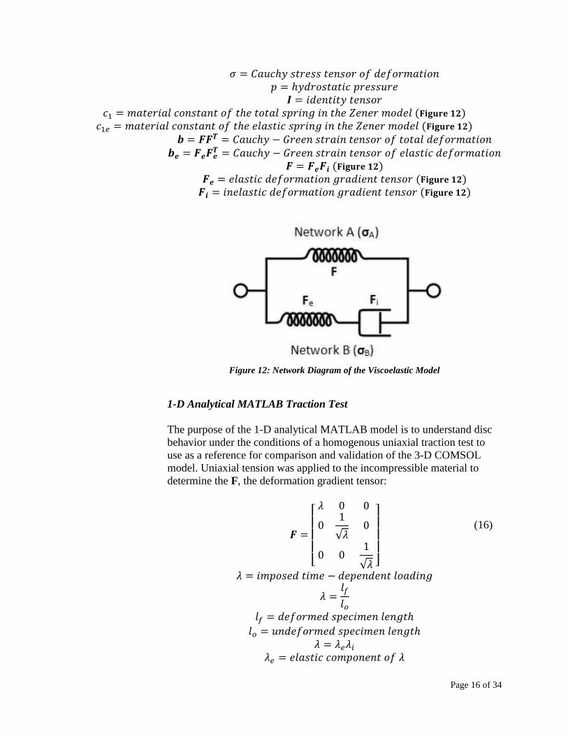
𝑭 = 𝑭𝒆𝑭𝒊 (𝐅𝐢𝐠𝐮𝐫𝐞 𝟏𝟐)

𝑭𝒆 = 𝑒𝑙𝑎𝑠𝑡𝑖𝑐 𝑑𝑒𝑓𝑜𝑟𝑚𝑎𝑡𝑖𝑜𝑛 𝑔𝑟𝑎𝑑𝑖𝑒𝑛𝑡 𝑡𝑒𝑛𝑠𝑜𝑟 (𝐅𝐢𝐠𝐮𝐫𝐞 𝟏𝟐)

𝑭𝒊 = 𝑖𝑛𝑒𝑙𝑎𝑠𝑡𝑖𝑐 𝑑𝑒𝑓𝑜𝑟𝑚𝑎𝑡𝑖𝑜𝑛 𝑔𝑟𝑎𝑑𝑖𝑒𝑛𝑡 𝑡𝑒𝑛𝑠𝑜𝑟 (𝐅𝐢𝐠𝐮𝐫𝐞 𝟏𝟐)

Figure 12: Network Diagram of the Viscoelastic Model

1-D Analytical MATLAB Traction Test

The purpose of the 1-D analytical MATLAB model is to understand disc

behavior under the conditions of a homogenous uniaxial traction test to

use as a reference for comparison and validation of the 3-D COMSOL

model. Uniaxial tension was applied to the incompressible material to

determine the F, the deformation gradient tensor:

𝑭 =

[

𝜆 0 0

01

√𝜆0

0 01

√𝜆

]

𝜆 = 𝑖𝑚𝑝𝑜𝑠𝑒𝑑 𝑡𝑖𝑚𝑒 − 𝑑𝑒𝑝𝑒𝑛𝑑𝑒𝑛𝑡 𝑙𝑜𝑎𝑑𝑖𝑛𝑔

𝜆 =𝑙𝑓

𝑙𝑜

𝑙𝑓 = 𝑑𝑒𝑓𝑜𝑟𝑚𝑒𝑑 𝑠𝑝𝑒𝑐𝑖𝑚𝑒𝑛 𝑙𝑒𝑛𝑔𝑡ℎ

𝑙𝑜 = 𝑢𝑛𝑑𝑒𝑓𝑜𝑟𝑚𝑒𝑑 𝑠𝑝𝑒𝑐𝑖𝑚𝑒𝑛 𝑙𝑒𝑛𝑔𝑡ℎ

𝜆 = 𝜆𝑒𝜆𝑖

𝜆𝑒 = 𝑒𝑙𝑎𝑠𝑡𝑖𝑐 𝑐𝑜𝑚𝑝𝑜𝑛𝑒𝑛𝑡 𝑜𝑓 𝜆

(16)

Page 17 of 34

𝜆𝑖 = 𝑖𝑛𝑒𝑙𝑎𝑠𝑡𝑖𝑐 𝑐𝑜𝑚𝑝𝑜𝑛𝑒𝑛𝑡 𝑜𝑓 𝜆

The MATLAB code computes λ, F, σA (Figure 12) at the beginning of

each time step. Then the previous value of λi is used to calculate λe. The

elastic component provides the Fe tensor, which is used to estimate σB

(Figure 12). After applying the Euler method for solving first-order

ordinary differential equations (ODEs), the code determines a new

inelastic deformation gradient tensor (Fi) and a new λi. When the final

value of λi is determined to be within the error limit compared to the

previous λi, the test is complete [5]. Appendix B of “A First Step towards

the Modeling of Intervertebral Disc Tissue Reconstruction” contains a full

listing of the MATLAB code used for this test.

This model characterizes the three material parameters for nonlinear

viscoelasticity: c1, c1e, and η. From these parameters, two characteristic

times are defined to separate the purely viscous response (equation (17))

from the elastic response (equation (18)):

𝜏𝑒 =𝜂

𝑐1𝑒= 𝑡𝑖𝑚𝑒 𝑡𝑜 𝑝𝑢𝑟𝑒𝑙𝑦 𝑣𝑖𝑠𝑐𝑜𝑢𝑠 𝑟𝑒𝑠𝑝𝑜𝑛𝑠𝑒

𝜏 =𝜂

𝑐1= 𝑡𝑖𝑚𝑒 𝑡𝑜 𝑒𝑙𝑎𝑠𝑡𝑖𝑐 𝑟𝑒𝑠𝑝𝑜𝑛𝑠𝑒

For a given triangular strain history, the code output results for τ, τe, and η,

which are displayed in Figures 13-15 [5].

Figure 13: Influence of Parameter τ for c1e = 0 and ɳ = 1 [5]

(17)

(18)

Page 18 of 34

Figure 14: Influence of Parameter τe for c1 = 0 and ɳ = 1 [5]

Figure 15: Influence of Parameter ɳ for c1 and c1e = 1 [5]

Based on these trends, c1 (Figure 13) provides global stiffness and

instantaneous response; whereas, c1e (Figure 14) and η (Figure 15)

determine the viscoelastic behavior [5].

Page 19 of 34

3-D and Axisymmetric 2-D COMSOL Models

COMSOL Multiphysics software was leveraged in this viscoelastic

analysis for finite element modeling. Appendix A of “A First Step towards

the Modeling of Intervertebral Disc Tissue Reconstruction” contains a

detailed listing of specific expressions implemented in the COMSOL

model. The models implemented in this analysis represent a

homogeneous, incompressible intervertebral disc of cylindrical shape.

Additionally, the 2-D model reflects an axisymmetric geometry (Table 2).

Analysis for this case determines only the stresses and deformation in the r

and z directions [5].

Table 2: Intervertebral Disc Dimensions for 2-D Axisymmetric COMSOL Model

Parameter Value Units

Nucleus Pulposus Radius 12 mm

Disc Radius 23 mm

Disc Height 12 mm

To simulate the axisymmetric 2-D case in COMSOL, the following

boundary conditions were applied:

r direction: constrain nodes along the axis of symmetry

r direction: constrain nodes along the vertebral end plates (top and

bottom)

z direction: constrain the bottom, rigid and fixed

Two sets of three material parameters (c1, c1e, and η) defined the

incompressible disc, one set each for the nucleus pulposus and the annulus

fibrosus [5].

When a characteristic time of ten seconds and all material parameters set

to equal one, COMSOL produced results for both the disc pressure

distribution and its von Mises stress distribution, shown in Figure 16 and

Figure 17, respectively.

Page 20 of 34

Figure 16: Pressure Distribution within the Intervertebral Disc [5]

Figure 17: von Mises Stress Distribution within the Intervertebral Disc [5]

Then, elastic parameters were assigned to the annulus fibrosus and

viscoelastic parameters were assigned to the nucleus pulposus (Table 3) in

order to simulate the force responses within the intervertebral disc.

Table 3: Material Constants for COMSOL Simulation

𝒄𝟏𝒆𝑨𝑭

𝜼𝑨𝑭 𝒄𝟏𝑨𝑭 𝒄𝟏

𝑵𝑷

0.0001 1 1 0.001

Page 21 of 34

This study outlined three series of simulations performed in COMSOL.

The first series did not converge; meanwhile, the second and third series

show a nearly perfect elastic response, which does not reflect the reality of

disc mechanics. Figure 18 indicates that the force response of the nucleus

pulposus contributes minimally to the total response in the intervertebral

disc [5]. Potential causes of this issue, as well as limitations of these

models is discussed in section 4.1.1.

Figure 18: Annulus Fibrosus (AF) and Nucleus Pulposus (NP) Relative Contributions

to the Intervertebral Disc (IVD) Resultant Force [5]

Results displayed in Figure 18 were based on the parameters contained in

Table 4.

Table 4: COMSOL Simulation Parameters for the Nucleus Pulposus

𝜼𝑵𝑷 𝝉𝑵𝑷 𝒄𝟏𝒆𝑵𝑷 𝝉𝒆

𝑵𝑷

0.01 10 1 0.01

3.2 Ligament Models

As discussed in section 2.1.3, seven ligaments are frequently used in numerical

models of the spine. However, many analyses do not model the ligaments at all.

Studies generally relating to the spine and problems in spine mechanics do not

generally focus on the effects of the ligaments or the loads they carry. The

Page 22 of 34

previously discussed models of the intervertebral disc (sections 3.1.1 and 3.1.2)

focused solely on the disc structure and not on the spine as a whole; therefore,

those analyses did not attempt to model any of the ligamentous components. In

consideration of the analysis methods utilized for interbody device design

(sections 3.3 and 3.4), there are a variety of approaches for modeling the

ligaments:

Absent – no ligaments are included in the numerical analysis [7]

Nonlinear springs

2 node or 3-D truss elements [6]

3.3 Multiscale Optimization

In a 2015 study, “Development of a Spinal Fusion Cage by Multiscale Modelling:

Application to the Human Cervical Spine,” a multiscale optimization approach

was attempted in order to enhance spinal fusion. Optimization focused on the

osteoconductivity (microstructure) and stiffness of the cage device. Constraints

on structure permeability are applied to obtain ideal device osteoconductivity. In

consideration of the cage stiffness, optimization considered the basic spine

motions of flexion, extension, bending, and axial rotation (section 2.1) [6].

Figure 19: Geometrical Model (C2-T1) [6]

A geometrical (Figure 19), finite element model (C2-T1) developed from CT

images of a healthy, adult subject formed the basis for this study. The spine

model included cortical and trabecular bone, the annulus fibrosus and nucleus

pulposus, and five ligaments (ALL, PLL, FL, ISL, and CL). Section 2.1 provides

further background on these biological components.

Page 23 of 34

Vertebrae and intervertebral disc structures were assumed to exhibit linear elastic

behavior and were modeled using tetrahedral elements in ABAQUS. Ligaments

were added to the model with 3-D truss elements that attached to their

corresponding anatomical insertion points through a coupling interaction. Figure

20 displays the finite element model via a 3-D visualization [6].

Figure 20: Finite Element Model (C2-T1) [6]

The desired result of this multiscale optimization is the idealized properties of a

linear, isotropic biomaterial that enhances vertebral fusion. A unit-cell of scaffold

material with a porous periodic microstructure is initially assumed prior to

executing the optimization. The objective is to optimize the structure on a global

scale (stiffness) and a micro-scale (osteoconductivity, material permeability), so a

two-scale optimization is arranged [6]:

𝑡 = 𝑡𝑟𝑎𝑐𝑡𝑖𝑜𝑛𝑠 𝑎𝑝𝑝𝑙𝑖𝑒𝑑 𝑡𝑜 𝑠𝑢𝑟𝑓𝑎𝑐𝑒

Γ = 𝑏𝑜𝑑𝑦 𝑠𝑢𝑟𝑓𝑎𝑐𝑒

𝑏 = 𝑏𝑜𝑑𝑦 𝑙𝑜𝑎𝑑𝑠

𝜌 = 𝑚𝑎𝑐𝑟𝑜 − 𝑠𝑐𝑎𝑙𝑒 𝑑𝑒𝑛𝑠𝑖𝑡𝑦

𝜇 = 𝑚𝑖𝑐𝑟𝑜 − 𝑠𝑐𝑎𝑙𝑒 𝑑𝑒𝑛𝑠𝑖𝑡𝑦

0 ≤ 𝜌 ≤ 1

0 ≤ 𝜇 ≤ 1

𝐻 = ℎ𝑜𝑚𝑜𝑔𝑒𝑛𝑖𝑧𝑒𝑑 𝑡𝑒𝑛𝑠𝑜𝑟

𝑃 = 𝑛𝑢𝑚𝑏𝑒𝑟 𝑜𝑓 𝑒𝑥𝑡𝑒𝑟𝑛𝑎𝑙 𝑙𝑜𝑎𝑑 𝑐𝑎𝑠𝑒𝑠

(19)

Page 24 of 34

𝛼 = 𝑤𝑒𝑖𝑔ℎ𝑡 𝑓𝑎𝑐𝑡𝑜𝑟𝑠

𝑌 = 𝑢𝑛𝑖𝑡 𝑐𝑒𝑙𝑙 𝑑𝑜𝑚𝑎𝑖𝑛

𝐸𝑖𝑗𝑘𝑙 = 𝐸𝑙𝑎𝑠𝑡𝑖𝑐 (𝑌𝑜𝑢𝑛𝑔′𝑠) 𝑚𝑜𝑑𝑢𝑙𝑢𝑠

𝐾 = 𝑠𝑡𝑖𝑓𝑓𝑛𝑒𝑠𝑠

�̅� = 𝑟𝑒𝑠𝑜𝑢𝑟𝑐𝑒 𝑐𝑜𝑛𝑠𝑡𝑟𝑎𝑖𝑛𝑡

When ρ or µ are equal to zero, a void is present. Conversely, ρ or µ equal to one

represents a solid space. ρ also takes intermediate, non-integer values that indicate

a prescribed volume fraction for the material. First, the inner problem of elasticity

must be solved using equation (20) for the homogenized elastic tensor [6].

𝐸𝑖𝑗𝑘𝑙𝐻 =

1

|𝑌|∫𝐸𝑝𝑞𝑟𝑠(𝜇) (𝛿𝑟𝑘 𝛿𝑠𝑙 −

𝜕𝜒𝑟𝑘𝑙

𝛿𝑦𝑠

) (𝛿𝑝𝑖𝛿𝑞𝑗 −𝜕𝜒𝑝

𝑖𝑗

𝛿𝑦𝑞

)𝑑𝑌

𝑌

𝑌 = 𝑢𝑛𝑖𝑡 𝑐𝑒𝑙𝑙 𝑑𝑜𝑚𝑎𝑖𝑛

|𝑌| = 1

In consideration of the set of six equilibrium equations in the Y domain, the

homogenized tensor is dependent on the micro-displacements χ, as described by

equation (21) [6].

∫𝐸𝑖𝑗𝑝𝑞(𝜇)𝜕𝜒𝑃

𝑘𝑙

𝑦𝑞

𝜕𝑤𝑖

𝜕𝑦𝑗 𝑑𝑌

𝑌

= ∫𝐸𝑖𝑗𝑘𝑙(𝜇)𝜕𝑤𝑖

𝜕𝑦𝑗 𝑑𝑌

𝑌

However, when the tensor depends instead on the elastic properties of the

microstructure, E is dependent on µ and follows the relationship in equation (22)

[6].

𝐸𝑖𝑗𝑘𝑙(𝜇) = 𝜇𝑃𝐸𝑖𝑗𝑘𝑙0

𝐸𝑖𝑗𝑘𝑙0 = 𝑒𝑙𝑎𝑠𝑡𝑖𝑐 𝑐𝑜𝑛𝑠𝑡𝑎𝑛𝑡 𝑜𝑓 𝑎 𝑠𝑜𝑙𝑖𝑑, 𝑙𝑖𝑛𝑒𝑎𝑟 𝑖𝑠𝑜𝑡𝑟𝑜𝑝𝑖𝑐 𝑚𝑎𝑡𝑒𝑟𝑖𝑎𝑙

After determining the material distribution from the inner optimization, it is used

as a constraint in the outer optimization problem, which deals with the

permeability of the material. The permeability tensor is orthotropic and given by

equation 23 [6].

𝐾𝑖𝑗𝐻 =

1

|𝑌| ∫𝐾𝑠𝑚 (𝛿𝑖𝑠 −

𝜕𝜒𝑖

𝜕𝑦𝑠)(𝛿𝑚𝑗 −

𝛿𝜒𝑗

𝛿𝑦𝑚) 𝑑𝑌

𝑌

An interpolation is then performed between permeability and the local density

via:

𝐾𝑖𝑚(𝜇) = (1 − 𝜇)𝑃 𝐾𝑖𝑚0 (𝜇)

𝐾0 = 𝑢𝑛𝑖𝑡𝑎𝑟𝑦, 𝑑𝑖𝑎𝑔𝑜𝑛𝑎𝑙, 𝑎𝑛𝑑 𝑖𝑠𝑜𝑡𝑟𝑜𝑝𝑖𝑐 𝑡𝑒𝑛𝑠𝑜𝑟

(20)

(21)

(22)

(23)

(24)

Page 25 of 34

This optimization is performed by sequentially calculating “the global and local

problem variables by the Method of Moving Asymptotes (MMA) and the

CONvex LINearization methods (CONLIN), respectively” [6]. The cage design

that results from this multiscale optimization proves to be useful for site-specific

scaffolds by accounting for both the overall spine behavior in flexion, extension,

lateral bending, and axial rotation and the site-specific boundary conditions.

3.4 Artificial Neural Networks

The use of artificial neural networks (ANN), as proposed by Nassau, et al, aims to

improve the computational efficiency of the cage design optimization process for

an ALIF cage. When finite element analysis (FEA) design inputs change, large

output changes result, which make FEA difficult to utilize for cage design

optimization. Traditional optimization methods are often computationally

intensive and inefficient. In the proposed design process, Taguchi statistical

methods and FEA combine with ANN to minimize the number of experimental

runs to optimize parameters for limiting potential fusion failure [7].

Figure 21: Design Process for ALIF Cage Design [7]

The first stage of the design process outlined in Figure 21 organizes the design

variables in a Taguchi framework. Taguchi statistical methods enable multiple

design variable modifications for each design in order to limit the number of

experimental runs and to improve the quality of the design. Used in combination

with FEA, this statistical method reduces the time spent during this stage of the

optimization process over that for traditional multiple linear regression [7].

Six design variables were arranged in the Taguchi matrix:

Cage material – analyzed within the property ranges for PEEK and

titanium

Ridge height – within the range of interface heights for commercially

available devices

Ridge width

Ridge oblique

Ridge rows – evenly spaced along the surface of the cage

Graft area

Page 26 of 34

A combination of SolidWorks 2011 and Abaqus/CAE 6.9 were used to perform

the FEA. Surface-to-surface frictionless contact interfaces were implemented with

no slip conditions with the cage positioned on the inferior vertebral body. A 1200

N uniform, compressive load was applied to the implant to simulate typical load

requirements for the lumbar spine. The parameters input for the FEA model are

summarized in Table 5 [7].

Table 5: FEA Input Parameters

Parameter Value Units

Poisson’s Ratio Cancellous Bone 0.3

Poisson’s Ratio Cortical Bone 0.3

Poisson’s Ratio Implant 0.3

Elastic Modulus Bone 137.5 MPa

Elastic Modulus 0.5 mm Partitioned Cortical Bone 12.0 GPa

Elastic Modulus Implant PEEK 3.6 GPa

Elastic Modulus Implant Ti6Al4V 110.0 GPa

Implant Height (constant, not including ridges) 6 mm

Implant Length 34 mm

Implant Width 26 mm

Bone Length 40 mm

Bone Width 40 mm

Bone Height 50 mm

Next, the ANN coding was implemented using Python version 2.7. In these

software simulations, a network of artificial neurons accomplishes a set task and

determines the cost of performing that task (output). According to Nassau, et al,

“ANNs can reduce the time and effort spent in model development and

computation time.” This process requires application of learning methods, which

include supervised, unsupervised, and reinforced learning. Since the design

variable inputs are determined from the combination of Taguchi statistical

methods and FEA, supervised learning is utilized [7].

The costs (outputs) used for learning are the maximal von Mises stresses on the

vertebra. Through the learning functions, the weights between variable

connections from the Taguchi matrix are updated. As shown in Figure 22, the

variable inputs (cage material, ridge height, ridge width, ridge oblique, ridge

rows, and graft area) represent individual neurons that are trained to reach the

single output neuron (von Mises stress) [7].

Page 27 of 34

Figure 22: Artificial Neural Network Process Diagram [7]

After 10,000 training executions in the ANN process, a solution was achieved at

30-45 minutes per model. Results from 30 models are presented in “Analysis of

Spinal Lumbar Interbody Fusion Cage Subsidence using Taguchi Method, Finite

Element Analysis, and Artificial Neural Network” with the final optimal result

shown here in Table 6.

Table 6: Final Result of ANN Analysis

Run

Cage Material

(GPa)

Ridge Height

(mm)

Ridge Width

(mm)

Ridge

Oblique (o)

Ridge

Rows

Graft Area

(mm2)

O3 3.600 1.400 1.000 104.000 11 224.000

4. Discussion

Each of the analyses summarized in section 3 utilizes a number of assumptions that

limit its use to a narrower range of specific scenarios of spine mechanics. These

analyses are often also limited by the available resources; however, limitations do not

make these models unimportant. Limitations of analyses may be overcome by

modifying assumptions, obtaining additional experimental data, refining the

simulations, or improving technology. Recommendations for future analysis of

intervertebral disc mechanics and for design of interbody fusion devices may increase

the range of problems in spine mechanics that may be studied using analytical and

numerical techniques.

Page 28 of 34

4.1 Model Limitations

4.1.1 Disc Model Limitations

Analytical Model of Intervertebral Disc Mechanics

The development of an analytical model for intervertebral disc mechanics

[4] relied on the assumption that the disc is axisymmetric. This assumption

precludes any models involving flexion or lateral bending, which are

typically asymmetric applications. Any deviation from horizontal, parallel

vertebral end plates that may be caused by disease, injury, or movement

also displays asymmetry such that this model must be modified.

This model also does not determine the specific interaction of the lamellae

in the annulus fibrosus. The model considers only two lamellae though the

annulus fibrosus contains 10-20 lamellae of alternating orientation. Disc

degeneration is caused by structural failure. In the annulus fibrosus,

circumferential tears, peripheral rim tears, and radial fissures cause

structural failure. The internal lamellae of the annulus may also buckle,

causing gross internal failure of the disc [1]. By simplifying the geometry

of the annulus fibrosus to produce an analytical model, rather than a

numerical one, this model is limited for studying the potential failure

conditions for intervertebral discs.

Viscoelastic Numerical Model of Intervertebral Disc Mechanics

The model of viscoelastic behavior of the intervertebral disc [5] produced

some unusual results that were not consistent with known disc behavior.

The model generated results that were almost perfectly elastic, which

indicates that the disc behavior is almost entirely governed by the annulus

fibrosus response. The author of the study included a validation of the

viscoelastic model in COMSOL to negate any concerns that the viscous

response was improperly modeled [5]. Rather, it is possible that the

annulus fibrosus model in COMSOL was too coarse and did not account

for the anisotropic structure of the lamellae.

During this study, a full sensitivity analysis could not be performed on the

parameters controlling the disc behavior. This posed convergence

difficulties for most of the simulations that were executed and yielded

unsatisfactory results [5]. Though direct application of these parameters

provided limited and unexpected results, further refinement and adjusted

parameters may improve the analysis.

Similar to the development of an analytical model of disc mechanics, this

model assumed that the disc exhibited axisymmetric geometry. Thus,

Page 29 of 34

adjustments would be required to analyze cases of flexion, extension, or

bending.

4.1.2 Multiscale Optimization Limitations

The multiscale optimization method explored in section 3.3 sought to

enhance bone fusion at the cage insertion site in the cervical spine. This

optimization resulted in an interbody fusion cage design of a biomaterial

that met requirements for osteoconductivity (permeability) and structural

strength [6]. A two-scale optimization with a full finite element model of

the cervical spine (C2-T1) is computationally strenuous, which limits the

simulation flexibility and complexity. The computational requirements

also impose time constraints for running simulations, which are important

considerations for the researcher.

Modeling trade-offs were required to reduce or limit the computational

strain of the simulations. To simplify the optimization model, linear elastic

properties were applied to the structures. This simplification and

assumption frequently appears in analytical and numerical treatment of

problems in spine mechanics.

4.1.3 Artificial Neural Networks Limitations

The use of artificial neural networks for analysis is limited by the amount

of data applied to the training iterations to increase the accuracy of the

program. Additional time spent generating data in the training runs to

increase the accuracy of the program restricts the time available for other

stages of the process or extends the analysis time. By extending the

analysis time, the efficiency of the ANN analysis decreases, thus negating

a major benefit of this analysis.

Due to significant differences in design for different types of interbody

fusion devices, results cannot be compared among a variety of devices.

This analysis specifically pertained to boxed ALIF interbody cages with

continuous ridges at the interface or surface contact points. The results

from this particular ANN procedure will not be directly comparable to

another.

Additionally, this study focused solely on the von Mises stress as the

critical parameter for predicted subsidence and failure of the graft. Other

parameters or other purposes for this analysis may be applied; however,

modifications would need to be made. For instance, the training

procedures and functions would likely differ from those used in this

analysis, and the variables represented by the neurons may be entirely

different to achieve new objectives. Though this process is not limited by

Page 30 of 34

any of these considerations, further investigation is needed to establish and

validate additional models.

4.2 Future Analysis Opportunities

4.2.1 Disc Analysis

Future study into the mechanical response of intervertebral discs that

analyzes cases of bending, asymmetric, or non-uniform loads would

advance the understanding of disc behavior in damaged or diseased spinal

columns. Many studies, including the two outlined in section 3.1, assume

a healthy disc that displays axisymmetric geometry under a uniform

compressive load. These simplifications create a simpler problem that can

be solved analytically or numerically.

Analytical problems generally involve simplifying assumptions,

particularly regarding geometry. Numerical methods provide the ability to

quickly analyze complex geometries but may involve assumptions for the

material parameters at each node. A combination of both techniques gives

insight into different aspects of disc behavior.

The viscoelastic model reviewed here (section 3.1.2), involved

simplifications to eliminate modeling complications due to the anisotropy

of the annulus fibrosus. Disc failure occurs due to buckling or tearing in

the lamellae of the annulus fibrosus, so this component of the disc is

critical to an accurate model of disc mechanics. To fully understand why

discs fail more often in people diagnosed with spinal diseases such as

scoliosis and spondylolisthesis, researchers and physicians need to

examine the annulus in detail through simulations that more closely reflect

experimental disc responses. The disc response in this study did not

display the expected viscoelasticity that is known to occur in intervertebral

disc experiments. Other constitutive viscoelastic relationships should be

investigated to determine the most appropriate for modeling disc

responses.

Further experimentation may be performed on intervertebral discs,

particularly of the lumbar region. Experimental results reflecting disc

behavior provide a source against which to validate analytical and

experimental models. Previous experimentation regarding the

intervertebral discs, as discussed in the development of an analytical

model by McNally and Arridge [4], required sectioning the disc to

experimentally test the annulus fibrosus, which destroys its load bearing

capability. New experimental techniques or imaging technologies may

help to increase knowledge of actual disc response and may provide

additional data to validate against for mathematical simulations.

Page 31 of 34

4.2.2 Interbody Device Design

Section 3.3 discussed the application of a two-scale design optimization

for cervical interbody fusion cage design. This multiscale optimization

approach enhanced the effect of fusion (osteoconductivity) and satisfied

the structural requirements for load bearing. Optimal parameters for a

biomaterial for cage construction resulted from the intensive analysis.

However, the analysis is computationally inefficient and time consuming.

The computational efficiency of the model may be investigated further to

determine improvements in handling the optimization. One simplification

that was introduced into the analysis [6] was that all structures display

linear elastic behavior. Though this assumption is common throughout

spine mechanics literature, greater insight may be gained through more

complex modeling of the material parameters for each structure. Due to

this additional complexity, the optimization would, however, be less

efficient and significantly more time intensive. Before adjusting the

model, a cost-benefit analysis should be performed to determine the

advantage of increased complexity and model refinement.

This interbody fusion cage design development pertained specifically to

the cervical region of the spine. Future extension of this study could apply

this same design process to interbody cages for the lumbar region, where

the bone structures and load bearing requirements differ from that of the

cervical region. Resulting designs and optimal material parameters may

then be compared to those for commercially available devices to quantify

the magnitude of any improvement this optimization process yields.

Future investigation of the application of artificial neural networks (ANN)

could extend the analysis to cages of other design. The same process may

be applied to determine the optimal parameters to minimize the probability

for fusion failure for PLIF and TLIF cages. The geometry of these cages

differs from that of the ALIF cage modeled in the study by Nassau, et al

[7]. These cages also generate possible undesirable issues for the patient

other than fusion failure. Additional modeling could incorporate multiple

objectives (costs, outputs) to analyze simultaneously using the ANN. This

process provides increased computational efficiency for analyzing

multiple objectives compared to the multiscale optimization method.

4.3 Summary

Four state of the art approaches to solving problems in spine mechanics were

summarized in this literature review. Two of these focused on problems in

intervertebral disc mechanics; while, the remaining studies presented state of the

art methods for optimizing interbody fusion cage design through the use of

Page 32 of 34

multiscale optimization and artificial neural networks. Each of these analyses

were limited by assumptions, such as axisymmetric structures and linear elastic

material properties for all components. In particular, the development of an

analytical model for disc mechanics assumed an axisymmetric disc under a

uniform compressive load, which makes this model unsuitable to study cases of

bending or asymmetric loading due to spinal disease, as in the case of scoliosis.

Other limiting conditions included computational efficiency of the method and

time. These conditions required simplifications and tradeoffs to be made in order

to generate significant results. In the case of artificial neural networks, a single

objective was pursued in favor of computational efficiency, rather than delving

into a more time consuming analysis with multiple objectives and additional

iterations. Even considering the typical limitations of analytical and numerical

analyses, these models form a basis further extension and research into spine

mechanics.

Page 33 of 34

References

1. Adams, M. A. (2013). The biomechanics of back pain (3rd ed.). Edinburgh, NY: Churchil

Livingstone.

2. Wang, X. (2013). Development of a computationally efficient finite element model of the

human spine for the purpose of conducting parametric studies of the stresses

induced in the spine and in spinal fusion instrumentation hardware during flexion,

torsion and extension. Raleigh, NC: North Carolina State University.

3. The ABCs of spinal fusion surgery: ALIF, PLIF, and TLIF. (n.d.). Retrieved April 24,

2016, from University Spine Center website:

http://www.universityspinecenter.com/the-abcs-of-spinal-fusion-surgery-alif-plif-

and-tlif

4. McNally, D. S., & Arridge, R. G. (1995). An analytical model of intervertebral disc

mechanics. Biomechanics, 28(1), 53-68. http://dx.doi.org/10.1016/0021-

9290(95)80007-7

5. Brulliard, V. (2010, May). A first step towards the modeling of intervertebral disc tissue

reconstruction.

6. Coelho, P. G., Fernandes, P. C., Folgado, J., & Fernandes, P. R. (2015). Development of

a spinal fusion cage by multiscale modelling: Application to the human cervical

spine. Procedia Engineering, 110, 183-190.

http://dx.doi.org/10.1016/j.proeng.2015.06.183

7. Nassau, C. J., Litofsky, N. S., & Lin, Y. (2012). Analysis of spinal lumbar interbody

fusion cage subsidence using Taguchi method, finite element analysis, and

Page 34 of 34

artificial neural network. Mechanical Engineering, 7(3), 247-255.

http://dx.doi.org/10.1007/s11465-012-0335-2