Lissajous and Fourier knots

Marc Soret and Marina Ville

Abstract

We prove that any knot of R3 is isotopic to a Fourier knot of type(1, 1, 2) obtained by deformation of a Lissajous knot.

1 Introduction

Fourier knots are closed embedded curves whose coordinate functions arefinite Fourier sums. Lissajous knots (defined in [BHJS]) are the simplestexamples : each coordinate function consists in only one term. Lissajousknots are Fourier knots of type (1,1,1) (cf. for example [K], [La2],[T]).

Surprisingly - at least at first sight - not every isotopy class of knots canbe represented by Lissajous knots. Indeed Lissajous knots are isotopic totheir mirror image; in particular a nontrivial torus knot cannot be isotopicto a Lissajous knot.

Let us first recall how to construct knots from a knot shadow.A knot shadow is a generic projection of a knot on a plane. It is a closed

planar curve with nodes, i.e. double points. Conversely given a shadow - i.e.an oriented planar closed curve with double points :

D : t 7→ γ(t) = (x (t) , y (t)) ∈ R2,

we can construct a knot in R3 by defining a height function z which has theright values at each node of the shadow. The knot is then defined by:

K : t 7→ (x (t) , y (t) , z (t)) ∈ R3.

Thus a Lissajous knot projects onto a Lissajous shadow (x(t) and y(t) arecosine functions). Although we cannot represent any knot by a Lissajousknot, still any knot K is isotopic to a knot which projects onto a Lissajous

1

arX

iv:1

507.

0088

0v1

[m

ath.

GT

] 3

Jul

201

5

shadow ([La]). In other words one can choose D to be a Lissajous shadow butone cannot always choose z(t) = cos(pt+φ) as the height function. However,this is possible if the height function z is a Fourier sum of a non prescribedfinite number of terms (cf. for instance [K]).It was conjectured in [La2] that any knot can be presented by a Lissajousdiagram with a height function consisting of a Fourier sum with a fixednumber of terms or even, as it was suggested experimentally in [BDHZ],with a height function consisting of only two terms: namely

Theorem 1. Any knot in R3 is isotopic to a Fourier knot of type (1,1,2).

The technique of the proof of theorem 1 is inspired by a paper of [KP]and uses Kronecker’s theorem. Another key property of number theory thatwill also be used is related to the fact that the only rational values of sin 2πp

q-

for integers p and q- are only 0,±1,±1/2.The main idea goes as follows: given a knot K in a given isotopy class ofknots, we show that it can be presented by a Lissajous diagram with primefrequencies. We then deform the shadow so that nodes are in “general posi-tion”, i.e. their parameters are rationally linearly independent. This will bederived from the fact that the nodal curve of the deformation is skewed inthe parameter space of all nodes. We then find an integer n and real numberφ -small- such that the height function h(t) := cos [2nπ (t+ φ)] has the rightintersection signs for every two values of the parameter t corresponding toa node of the Lissajous shadow. The height function then defines a thirdcoordinate function which together with the deformed Lissajous shadow co-ordinates defines a curve of R3 in the given isotopy class.

The paper is organized as follows : In Section 2 and 3 we fix notations andterminology. We compute the node parameters of deformations of Lissajousplanar curves in section 4; we also show that any knot admits a Lissajousdiagram with prime frequencies.In Section 5, we show that the nodal curves of our deformations are skewed: for an appropriate choice of deformation parameters and a simple choice ofphases, we can compute the determinant of the k-th derivatives k = 1, · · · , nDof the nodal curve position vector in RnD and show that it is not zero. InSection 5.7, the determinant is expressed as a product of factors, each ofwhich is proved to be different from zero. We also show that the skewness ofthe nodal curve implies that nodes parameters of the diagram are rationallylinear independent for a dense subset of the deformation parameter. The lastsection is devoted to the proof of the theorem : Kronecker’s theorem applied

2

to Q-linear independence of nodal coordinates allows us to choose, as heightfunction of any knot represented by an appropriate Lissajous shadow, a cosinefunction with appropriate frequency.Acknowledgement : the starting point of this paper was a fruitful meetingwith P-V Koseleff whom we thank heartfully.

Contents

1 Introduction 1

2 Terminology 42.1 Knots in R3 . . . . . . . . . . . . . . . . . . . . . . . . . . . . 42.2 Deformation of a knot shadow and nodal curve . . . . . . . . . 4

3 Fourier Knots 53.1 Lissajous knots . . . . . . . . . . . . . . . . . . . . . . . . . . 53.2 Torus knots . . . . . . . . . . . . . . . . . . . . . . . . . . . . 6

4 Nodes and deformations of knot shadows 64.1 Lissajous Figures, nodes and symmetries . . . . . . . . . . . . 74.2 Nodes parameters of Lissajous planar curves . . . . . . . . . . 84.3 Prime knot diagrams . . . . . . . . . . . . . . . . . . . . . . . 104.4 Nodes coupling . . . . . . . . . . . . . . . . . . . . . . . . . . 114.5 Deformations of planar Lissajous curves . . . . . . . . . . . . 134.6 The nodal curve of a deformation of Lissajous curves . . . . . 13

5 Q-Linear dependence of the nodal curve coordinates 165.1 Infinitesimal deformation and Q-linear independence . . . . . 165.2 The Lissajous nodal curve is skewed . . . . . . . . . . . . . . . 175.3 General form of the nodal curve coordinates . . . . . . . . . . 175.4 Series expansion of nodal curves . . . . . . . . . . . . . . . . . 185.5 Series expansion of the nodal curve’s Wronskian . . . . . . . . 195.6 The Wronskian is not zero . . . . . . . . . . . . . . . . . . . . 215.7 The lowest order term D0 of the Wronskian is not zero . . . . 245.8 Q-linear dependence of nodal curves coordinates . . . . . . . . 27

6 Proof of the Theorem 286.1 Kronecker’s theorem . . . . . . . . . . . . . . . . . . . . . . . 29

3

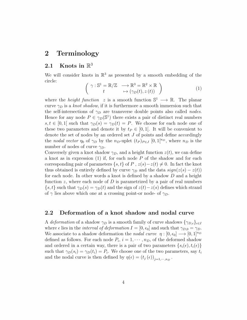
2 Terminology

2.1 Knots in R3

We will consider knots in R3 as presented by a smooth embedding of thecircle: (

γ : S1 = R/Z −→ R3 = R2 × Rt 7→ (γD(t), z (t))

)(1)

where the height function z is a smooth function S1 −→ R. The planarcurve γD is a knot shadow, if it is furthermore a smooth immersion such thatthe self-intersections of γD are transverse double points also called nodes.Hence for any node P ∈ γD(S1) there exists a pair of distinct real numberss, t ∈ [0, 1[ such that γD(s) = γD(t) = P . We choose for each node one ofthese two parameters and denote it by tP ∈ [0, 1[. It will be convenient todenote the set of nodes by an ordered set J of points and define accordinglythe nodal vector η0 of γD by the nD-uplet (tP )P∈J [0, 1[nD , where nD is thenumber of nodes of curve γD.Conversely given a knot shadow γD, and a height function z(t), we can definea knot as in expression (1) if, for each node P of the shadow and for eachcorresponding pair of parameters {s, t} of P , z(s)−z(t) 6= 0. In fact the knotthus obtained is entirely defined by curve γD and the data sign(z(s)− z(t))for each node. In other words a knot is defined by a shadow D and a heightfunction z, where each node of D is parametrized by a pair of real numbers{s, t} such that γD(s) = γD(t) and the sign of z(t)−z(s) defines which strandof γ lies above which one at a crossing point-or node- of γD.

2.2 Deformation of a knot shadow and nodal curve

A deformation of a shadow γD is a smooth family of curve shadows {γD,ε}ε∈Iwhere ε lies in the interval of deformation I = [0, ε0] and such that γD,0 = γD.We associate to a shadow deformation the nodal curve η : [0, ε0] −→ [0, 1]nD

defined as follows. For each node Pi, i = 1, · · · , nD, of the deformed shadowand ordered in a certain way, there is a pair of two parameters {si(ε), ti(ε)}such that γD(si) = γD(ti) = Pi. We choose one of the two parameters, say tiand the nodal curve is then defined by η(ε) = (tj (ε))j=1,··· ,nD .

4

3 Fourier Knots

We give a quick reminder of some geometric knot presentations that are ofsome interest in our topic: Fourier knots, Lissajous knots and torus knotsthat all belong to next family.A Fourier knot -of type (m,n, p)- is a parametrized curve of R3 defined by :

Fm,n,p :

([0, 1[ −→ R3

t 7→ Fm,n,p(t)

)(2)

with

Fm,n,p(t) =

(m∑i=1

Mi cos(2πmit+ φi),n∑i=1

Ni cos(2πnit+ ψi),

p∑i=1

Pi cos(2πpit+ τi)

)for some φi,Mi, Ni, ψi, , τi, Pi ∈ R and mi, ni, pi ∈ N.It was proved in [La2] that any knot K is isotopic to a curve of type (1, 1, nK)where nK depends on the knot.

3.1 Lissajous knots

Fourier knots of type (1, 1, 1) are also called Lissajous knots and have beenextensively studied in [BHJS]).

L(n1, n2, n3, φ1, φ2) :

([0, 1] −→ R3

t 7→ (cos 2πn1t, cos 2πn2 (t+ φ1) , cos 2πn3 (t+ φ2))

)(3)

It is noteworthy to recall that Lissajous knots are topologically equivalentto closed billiard trajectories in a cube. (cf. [JP]) These Lissajous knotsproject horizontally on planar Lissajous curves of type L(n1, n2, φ1).When the phase φ1 is zero, the Lissajous figure degenerates into a 2-1 curveC(n1, n2) which is a subset of an algebraic Chebyshev open curve as definedin [KP]:

T (n1, n2) = {(x, y) : Tn1(x) = Tn2(y) = 0},

where Tn is the Chebyshev polynomial of degree n (see fig. 1).Although not all knot are Lissajous knots, [KP] showed that, for suitablenumbers n1, n2, n3 and phase φ, any knot is isotopic a Chebyshev knot ob-tained by Alexandrov compactification of a curve T (n1, n2, n3, φ) : S1 −→ R3

with T (n1, n2, n3, φ)(t) = (Tn1(t), Tn2(t), Tn3(t+ φ)).

5

-1.0 -0.5 0.5 1.0

-1.0

-0.5

0.5

1.0

,

-1.0 -0.5 0.5 1.0

-1.0

-0.5

0.5

1.0

Figure 1: knot L(2, 3, 5, 0, .2, 2) = 61, shadow L(2, 3, .2), and associatedChebyshev figure C(2, 3)

3.2 Torus knots

Another key family of Fourier knots are torus knots -neither of which can beisotopic to a Lissajous knot (except the trivial ones)! A Torus knot T (p, q)is originally defined as an embedding of S1 onto a torus as a Fourier knot oftype (3, 3, 1) :

T (p, q)(t) =

(cos 2πqt

(1 +

1

2cos 2πpt

), sin 2πqt

(1 +

1

2cos 2πpt

), sin 2πpt

).

But it was shown in [H] that torus knots T (p, q)’s are isotopic to Fourierknots of type (1, 1, 2) :

T (p, q)(t) =

(cos 2πpt, cos 2πq

(t+

1

4p

), cos 2π

(pt+

1

4

)+ cos 2π

((q − p) t+

1

4p

))

4 Nodes and deformations of knot shadows

We first recall some basic properties of Lissajous planar curves and computethe positions of its nodes.In the second part of the section we add a small perturbation term to one ofthe two coordinates; we define a family of perturbed Lissajous planar curveswhich are very close to the original Lissajous figure. We then describe thepositions of the nodes as functions of the deformation parameter ε.

6

4.1 Lissajous Figures, nodes and symmetries

We need to give some precisions on the Lissajous curves :

L(n1, n2, φ) :

([0, 1] −→ R2

t 7→ (cos (2πn1t) , cos (2πn2t+ φ))

)(4)

We will suppose that n1 and n2 are coprime (otherwise L is not 1-1).We can also suppose for our purpose that the phase φ is a small positiveirrational number. Our first goal is to find the expression of the orderedpairs of parameters (ti, si), i = 1, · · ·N corresponding to the double pointsPi, i = 1, · · · , N of a Lissajous figure. In the degenerate case where the

(0,0) (2n1,0)

(0,2n2)

(n1,n2)

II

I-1.0 -0.5 0.5 1.0

-1.0

-0.5

0.5

1.0

,

-1.0 -0.5 0.5 1.0

-1.0

-0.5

0.5

1.0

Figure 2: 31 Nodes parametrized by integer points in triangle ∆ of LissajousL(4, 5, .1), and associated Chebyshev C(4, 5)

(0,0) (2n1,0)

(0,2n2)

(n1,n2)

I

II

1.0 0.5 0.5 1.0

1.0

0.5

0.5

1.0

Type I ,

-1.0 -0.5 0.5 1.0

-1.0

-0.5

0.5

1.0

Figure 3: 22 nodes parametrized by integer points of Lissajous curveL(3, 5, .1) with 10 nodes of type I, and associated Chebyshev C(3, 5)

phase φ is zero we obtain a 2− 1 curve (see figure 2 and 3). This curve is asubset of a Chebyshev curve defined in [KP] and which is an open algebraiccurve.

7

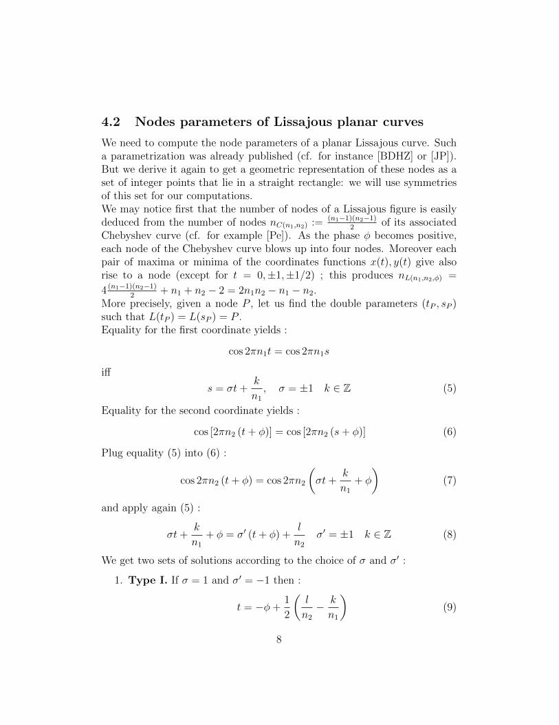
4.2 Nodes parameters of Lissajous planar curves

We need to compute the node parameters of a planar Lissajous curve. Sucha parametrization was already published (cf. for instance [BDHZ] or [JP]).But we derive it again to get a geometric representation of these nodes as aset of integer points that lie in a straight rectangle: we will use symmetriesof this set for our computations.We may notice first that the number of nodes of a Lissajous figure is easilydeduced from the number of nodes nC(n1,n2) := (n1−1)(n2−1)

2of its associated

Chebyshev curve (cf. for example [Pe]). As the phase φ becomes positive,each node of the Chebyshev curve blows up into four nodes. Moreover eachpair of maxima or minima of the coordinates functions x(t), y(t) give alsorise to a node (except for t = 0,±1,±1/2) ; this produces nL(n1,n2,φ) =

4 (n1−1)(n2−1)2

+ n1 + n2 − 2 = 2n1n2 − n1 − n2.More precisely, given a node P , let us find the double parameters (tP , sP )such that L(tP ) = L(sP ) = P .Equality for the first coordinate yields :

cos 2πn1t = cos 2πn1s

iff

s = σt+k

n1

, σ = ±1 k ∈ Z (5)

Equality for the second coordinate yields :

cos [2πn2 (t+ φ)] = cos [2πn2 (s+ φ)] (6)

Plug equality (5) into (6) :

cos 2πn2 (t+ φ) = cos 2πn2

(σt+

k

n1

+ φ

)(7)

and apply again (5) :

σt+k

n1

+ φ = σ′ (t+ φ) +l

n2

σ′ = ±1 k ∈ Z (8)

We get two sets of solutions according to the choice of σ and σ′ :

1. Type I. If σ = 1 and σ′ = −1 then :

t = −φ+1

2

(l

n2

− k

n1

)(9)

8

Hence

s = t+k

n1

= −φ+1

2

(l

n2

+k

n1

)(10)

Since s, t ∈ [0, 1[, the integer points (k, l) necessarily lie in a parallelo-gram P which is defined by conditions :{

2φn1n2 ≤ n1l − n2k < (1 + φ)2n1n2

2φn1n2 ≤ n1l + n2k < (1 + φ)2n1n2(11)

As phase φ is small, parallelogram P is obtained by a small translationof the parallelogram with vertices (0, 0), (n1, n2), (−n1, n2), (0, 2n2). Sincen1 and n2 are coprime there are only the 4 integer points vertices onthe boundary of the translated parallelogram.

2. Type II. In the second case, σ = −1, σ′ = 1 and we obtain :

t =1

2

(k

n1

− l

n2

)(12)

Hence

s =1

2

(l

n2

+k

n1

)(13)

And conditions s, t ∈ [0, 1[ yields - we recall that φ is very small-{0 ≤ n2k − n1l < 2n1n2

0 ≤ n2k + n1l < 2n1n2(14)

Solutions are given by integer points (k, l) ∈ P ′ which is a small transla-tion of the parallelogram with vertices (0, 0), (n1, n2), (n1,−n2), (2n1, 0).

For each solution found, one should check that s 6= t and also that pairs{t, s} corresponding to the same node are not counted twice.For each pair of solutions {s, t}, condition s 6= t implies k 6= 0 for thefirst type and l 6= 0 in the second case; furthermore for points of type Ithe transformation : k 7→ −k permutes t and s which are parameters thatcorrespond to the same node. Hence we can reduce the parameter set ofnodes to the isosceles triangle ∆I := {(k, l) ∈ P : k > 0} and similarly fortype II points : ∆II := {(k, l) ∈ P ′ : l > 0}. In The union of ∆I and ∆II

defines a straight triangle ∆ (see figure 5 a)). In summary :

9

Lemma 1. A generic Lissajoux planar curve L(n1, n2, φ), with n1 and n2

coprime and φ small, and defined by

L(n1, n2, φ) :

([0, 1] −→ R2

t 7→ (cos 2πn1t, cos [2πn2 (t+ φ)])

)(15)

has nL(n1,n2,φ) = 2n1n2 − n1 − n2 nodes parametrized by the integer pointsthat lie in the interior of the straight triangle ∆ :J = ∆ ∩ N× N := {(k, l) : k > 0, l > 0, n2k + n1l < 2n1n2}.The node vector is by definition (tj)j∈J ∈ [0, 1[nL(n1,n2,φ) where,for each (k, l) ∈ J :

tkl :=

−φ+ 12

(− kn1

+ ln2

)if n1l > n2k (type I)

12

(kn1− l

n2

)if n1l < n2k (type II)

(16)

4.3 Prime knot diagrams

Figure 4: C(4, 5), billiard curve L(4, 5, .1) and plat-closure braid of L(4, 5, .1)

We first recall that a checkerboard - such as L(n1, n2)- is the plat-closure(cf. [B]) of a braid of 2n1 strands defined by the following group element ofthe braid group B2n1 :

C(2n1, n2 − 1) :=(σ∗2σ

∗4 · · ·σ∗2n1−2σ

∗1σ∗3 · · · σ∗2n1−1

)n2−1σ∗2σ

∗4 · · ·σ∗2n1−2

(the powers of σi, denoted by∗ are ±1; they are irrelevant as far as the shadowis concerned).

10

C. Lamm showed in his thesis (cf [La2] Theorem 2.3) that any knot ispresented by a checkerboard diagram Ck(2n1, 2n1.p) for some p. This diagramhas a Lissajous shadow of type L(n1, n2 = 2n1p + 1). Hence we can as wellsay that any knot is presented by a Lissajous diagram.

Proposition 1. Any knot admits a Lissajous diagram with shadow L(n1, n2)where n1 and n2 are odd primes and where n2 ≡ 1 mod n1.

Proof : the only constraint on n1 is that it should be greater or equal tothe braid index of K. In particular choosing n1 large enough, we can sup-pose that n1 is prime and odd. Moreover from the proof of theorem 2.3of [La2], we can also represent the same knot by diagrams with shadowsL(n1, n2 = 2n1(p + q) + 1) for any nonnegative number q: q represents thenumber of pure braids added to the original rosette braid. For each addedpiece and by a judicious choice of the crossing numbers the new rosette braidrepresents the same knot. By Dirichlet’s prime number theorem and since2n1 and n2 are rel. prime, there are numbers q such that n2 is prime. Wewill thus restrict our further investigation of the Lissajous figure to the casewhere n1 and n2 are odd primes.

4.4 Nodes coupling

(0,0) (2n1,0)

(0,2n2)

(n1,n2)I

II

(0,0) (2n1,0)

(0,2n2)

(n1,n2)

I

II

V

II

V

I

Figure 5: Triangle ∆ = ∆I ∪∆II ; hor. and vert. symmetries

We describe a method to pair the nodes which will be crucial in section 5.

We will regroup integer points of the triangle ∆, described in Lemma1, by pairs. The n1n2 − n2 nodes of type I (resp. the n1n2 − n1 nodes of

11

type II) are parametrized by the integer points of the isoceles subtriangle∆I := ((0, 0) , (n1, n2) , (0, 2n2)) ⊂ ∆-resp. ∆II := ((0, 0) , (2n1, 0) , (n1, n2)) ⊂ ∆- (see fig 5) .

(0,0) (2n1,0)

(0,2n2)

(n1,n2)I0

I'

I''

(0,0) (2n1,0)

(0,2n2)

(n1,n2)

I

II

Figure 6: Subdomains of triangle ∆

Lemma 2. Each node of ∆I (resp. ∆II) is coupled to a different node of ∆I

(resp. ∆II). The set of pairs extracted from ∆I (resp. ∆II) are parametrizedby integer points lying in the parallelograms :ΠI :=

((0, 0) ,

(n1

2, n2

2

),(n1

2, n2 + n2

2

), (0, n2)

)(resp. ΠII :=

((0, 0) ,

(n1

2, n2

2

),(n1 + n1

2, n2

2

), (n1, 0)

))(see figure 5).

Proof :

1. We first regroup separately integer points in each isosceles triangle,namely ∆I and ∆II , using resp. the horizontal symmetry σIh : (k, l) −→(n1 − k, l) (resp. symmetry σIIh : (k, l) −→ (k, n2 − l)).We pair each integer point above the axis of symmetry with its reflectionimage. Notice that, since n1 and n2 are odd, no integer point lies on theaxis of σIh (resp. σIIh ). Hence this process forms pairs of distinct pointsparametrized by integer points in the isosceles triangle (see fig.6)∆I0 := ((0, n2) , (n1/2, n2/2) , (n1/2, 3n2/2)).(resp. ∆II0 := ((n1, 0) , (n1/2, n2/2) , (3n1/2, n2/2))).

2. The remaining points of ∆I that are not yet coupled, form two isoscelessubtriangles ∆I′ ,∆I′′ -resp ∆II′ ,∆II′′ of ∆II- (see figure 5).We then couple each point of ∆I′ with a point of ∆I′′ (resp. each pointof ∆II′ with a point of ∆II′′) via a translation τ I of vector (0, n2) (resp.via a translation τ II of vector(n1, 0) (see fig. 6).

12

Alltogether the set of pairs of nodes are parametrized by the union of twoparallelograms ΠI := ∆I′ ∪∆I0 and ΠII := ∆II′ ∪∆II0 .

4.5 Deformations of planar Lissajous curves

Let us consider a deformation of a Lissajous figure {Lε(n1, n2, n3, φ, ψ)}ε∈[0,ε0[

Lε(n1, n2, n3, φ, ψ) :

([0, 1] −→ R2

t 7→ (cos (2πn1t) , cos (2πn2 (t+ φ)) + ε cos (2πn3 (t+ φ+ ψ)))

)These are Fourier curves of type (1, 2). The node positions of the curve areshifted as we can see in figure 6 and the symmetry of the initial Lissajousfigure is clearly broken.

-1.0 -0.5 0.5 1.0

-1.0

-0.5

0.5

1.0

-1.0 -0.5 0.5 1.0

-1.0

-0.5

0.5

1.0

Figure 7: Lissajous shadow L(4, 5, .1) and deformation Lε(4, 5, 7, .1, .2)

Let us compute the nodes parameters of these deformed Lissajous planarcurves.

4.6 The nodal curve of a deformation of Lissajous curves

Consider a deformation {Lε(n1, n2, n3, φ, ψ)}ε∈[0,ε0] where n1 and n2 are oddcoprimes.The coordinates of the nodal curve η introduced in section 2.2 are orderedaccording to the lexicographic ordering of integer points of the triangle ∆described in Lemma 1.We proceed as in this Lemma.

Suppose Lε(t) = Lε(s); then equality of first coordinates yields

s = σt+k

n1

, k ∈ Z, σ = ±1. (17)

13

Equality for the second coordinates yields :

cos (2πn2 (t+ φ))− cos (2πn2 (s+ φ)) =ε (cos(2πn3(s+ φ+ ψ))− cos(2πn3(t+ φ+ ψ)))

(18)

Or, using formula cos a− cos b = −2 sin(a+b2

) sin(a−b2

),

sin(2πn2

(t+s2

+ φ))

sin(2πn2

t−s2

)=

−ε sin(2πn3

(t+s2

+ φ+ ψ))

sin(2πn3

t−s2

).

(19)

Plug equality (17) into (19); we get two cases according to the value ofσ = ±1 :

1. Type I. If σ = +1 ; s = t + kn1

hence s+t2

= t + k2n1

, k ∈ Z and t isgiven implicitely by the equation :

sin

(2πn2

(t+

k

2n1

+ φ

))ak = ε sin

(2πn3

(t+

k

2n1

+ φ+ ψ

))(20)

where ak = −sin(πn2kn1

)sin(πn3kn1

) (which is well-defined and not zero since k < n1

and n2, n3 are prime relatively to n1).Hence for any ε, solutions are parametrized by the integer points (k, l) ∈∆I and given by

tkl(ε) := −φ+1

2

(− k

n1

+l

n2

)+ ukl(ε) (21)

where ukl is a function defined implicitely by fkl (ukl (ε)) = ε with :

fkl(y) = ak(−1)lsin 2πn2y

sin(

2πn3

(y + l

2n2+ ψ

))2. Type II. If σ = −1 then s = −t+ k

n1, hence t−s

2= t− k

2n1and

bk sin

(2πn2

(t− k

2n1

))= ε sin

(2πn3

(t− k

2n1

))(22)

where bk = −sin(

2πn2

(k

2n1+φ))

sin(

2πn3

(k

2n1+φ+ψ

)) (bk is not zero and well-defined for

small φ, ψ as for the ak’s).

14

As in case I, solutions are given by

tkl(ε) := +1

2

(k

n1

− l

n2

)+ uk,l(ε) (23)

with fkl (ukl (ε)) = ε where

fkl(y) = bk(−1)lsin 2πn2y

sin(

2πn3

(y + l

2n2

)) .Notice that ukl(0) = 0 and that the tkl(0) are the solutions of type I and IIdescribed in Lemma 1. Let us summarize these facts and define the nodalcurve of the deformation:

Lemma 3. Consider a deformation of planar Lissajous curves Lε(n1, n2, n3, φ, ψ)with n1 and n2 odd and consider a Lissajous deformation :

Lε(n1, n2, n3, φ, ψ) :

([0, 1] −→ R2

t 7→ (cos 2πn1t, cos [2πn2 (t+ φ)] + ε cos [2πn3 (t+ φ+ ψ)])

)ε ∈ [0, ε0[, where we suppose that ε0 and φ are small and n1, n2, n3 are rela-tively prime.Each planar curve Lε has nL(n1,n2,φ) = 2n1n2−n1−n2 nodes parametrized bythe integer points that lie in the interior of the straight triangle ∆ (definedin Lemma 1)The nodal curve η(ε) = (tkl)(k,l)∈∆ ∈ [0, 1[nL(n1,n2,φ) is defined by

η(ε)kl = tkl(ε) :=

−φ+ 12

(− kn1

+ ln2

)+ ukl(ε) if (k, l) ∈ ∆I

12

(kn1− l

n2

)+ ukl(ε) if (k, l) ∈ ∆II .

(24)

where the kl are lexicographically ordered.Functions ukl are the local inverse functions of functions fkl, ie such thatfkl ◦ ulk = Id.• If (k, l) ∈ ∆I then :

fkl(y) =sin 2πn2y

aIkl sin[2πn3

(y + l

2n2+ ψ

)] , aIkl := (−1)l+1sin π n3k

n1

sinπ n2kn1

• If (k, l) ∈ ∆II then :

15

fkl(y) =sin 2πn2y

aIIkl sin[2πn3

(y + l

2n2

)] , aIIkl := (−1)l+1sin[2πn3

(k

2n1+ φ+ ψ

)]sin[2πn2

(k

2n1+ φ)] .

5 Q-Linear dependence of the nodal curve co-

ordinates

5.1 Infinitesimal deformation and Q-linear independence

We will give a infinitesimal condition on the curve to ensure the rationallinear independence. But first let us prove

Lemma 4. Let γ : I = [0, ε0] −→ [0, 1]n be a real analytic skew curve. Thenthe set of ε ∈ [0, ε0] such that the numbers

γ1(ε), · · · , γn(ε), 1 (25)

are rationally linear independent, is dense in [0, ε0].

Proof : we exhibit a sequence of ε’s that converges to zero and such that thenumbers (25) are rationally linear independent-the same proof will work forany other points 6= 0.If such a sequence does not exist, there is a nonempty neighborhood I ′ of 0in I such that the coordinates of γ(ε) and 1 are rationally linear dependent;then

n∑i=1

λi(ε)γi(ε) + λn+1(ε) = 0.

Since I ′ is an uncountable set, the map λ : I ′ −→ Qn+1 takes the same vectorvalue (λi)i=1,··· ,n for infinitely many εk with lim

k 7→+∞εk = 0. Hence for infinitely

many values of εk converging to 0 we have

n∑i=1

λiγi(εk) + λn+1 = 0. (26)

Since γ is analytic we deduce that this relation is true for all ε; hence γ belongsto a hyperplane with rational coefficients, which contradicts the skewness ofcurve γ.Similarily we prove

16

Lemma 5. If t1, · · · , tn, 1 are rationally lin. independent, then {t1+φ, · · · , tn+φ, 1} are rationally linear independent for a dense subset of R.

Taking successive derivatives of equation (26) in Lemma 4 we deduce thefollowing infinitesimal criterion for Q-linear independence :

Corollary 1. Let γ : [0, ε0] −→ [0, 1]n be an analytic curve such that aWronskian is not zero :∣∣∣∣∣∣∣∣∣

γ(k1)1 (0) γ

(k2)1 (0) . . . γ

(kn)1 (0)

γ(k1)2 (0) γ

(k2)2 (0) . . . γ

(kn)2 (0)

...... . . .

...

γ(k1)n (0) γ

(k2)n (0) . . . γ

(kn)n (0)

∣∣∣∣∣∣∣∣∣ 6= 0 (27)

where k1 < k2 < · · · , kn; then the set of real numbers {1, γj(ε), j = 1, · · · , n}are linear independent over Q for a dense subset of [0, ε0].

5.2 The Lissajous nodal curve is skewed

We will show in this section that

Proposition 2. Assume that n1, n2 are odd primes and n3 is relatively primeto n1, n2 and satisfy : {

n3 ≡ 2 mod n1

n3 ≡ 2 mod n2.(28)

Then there are positive real numbers ε0, φ0, ψ0 such that for any |ε| ≤ ε0,|φ| ≤ φ0, |ψ − π

4| ≤ ψ0, the nodal curve η(ε) of the Lissajous deformation

Lε(n1, n2, n3, φ, ψ) is skewed.

In Subsection 5.3 we give an explicit expression of the nodal coordinates ofa Lissajous deformation; we then show, in Subsection 5.5, that the WronskienD of the nodal curve is a polynomial in r = n2

n3; in Subsection 5.7 we compute

the coefficient D0 of the lowest order monomial.

5.3 General form of the nodal curve coordinates

Consider a curve Y :

Y :

(I := [0, ε0] −→ Rn

ε 7→ (yj)j∈J

)(29)

17

with initial position Y (0) = (yj (0))j=1,··· ,n and let us define curve U suchthat Y = Y (0) + U. Then :

yj(ε) = yj(0) + uj(ε) and uj(0) = 0 ∀ε ∈ I, j = 1, · · · , n.

For each j = 1, · · · , n, the j-th coordinate function uj of U is defined as theinverse function of a given function fj :

fj(uj(ε)) = ε ∀ε ∈ I.

Though each coordinate function uj(ε)- which we will denote indistinctivelyby u(ε)- is defined implicitely, the Lagrange inversion formula (cf. for instance[S]) yields an explicit power series expansion in terms of ε in the neigborhoodof any 0 :

u(ε) :=∑n≥1

un(0)εn

n!

Namely :

u(ε) =∞∑n=1

d(n−1)

dtn−1

(t

f(t)

)n∣∣∣∣t=0

εn

n!. (30)

5.4 Series expansion of nodal curves

Each one of the coordinates of the nodal curve of a Lissajous deformation isdefined by the inverse of a real function of the following type :

f(u) =sinu

a sin(ru+ ψ)(r ∈ Q, a ∈ R∗, ψ ∈ R). (31)

A simple computation using Lagrange’s inverse formula (30) (cf. for example[S]) gives the coefficients un(0) of the expansion around zero of u such thatf ◦ u = Id:

u1(0) = a sinψ, u2(0) = a2r sinψ cosψ, , u3(0) = a3 sinψ(6r2 + (1− 9r2) sin2 ψ

)· · · .

Lemma 6. Let u be the inverse function of f defined by equation (31).For each n ≥ 1 the n-th coefficient of the power series of u around zero :un equals anPn(sinψ, cosψ, r), where Pn is a polynomial of degree n w.r.t.

18

variables cosψ and sinψ. Pn is also a polynomial in r of degree n− 1 whoselowest order term is:

un(0) :=

an(

ysinu

)n∣∣∣∣(n−1)

u=0

sinn ψ := ancn sinn ψ (n odd),

r.nan( ysinu

)n∣∣∣∣(n−2)

u=0

cosψ sinn−1 ψ := ancn cosψ sinn−1 rψ (n even)

(32)

Proof : Lagrange’s inversion formula (30) applied to function (31) andevaluated at zero, yields :

un(0) = an((

y

sin y

)nsinn (ry + ψ)

)∣∣∣∣(n−1)

y=0

Leibniz formula yields :

un(0) = ann−1∑k=0

(n− 1

k

)[(y

sin y

)n]∣∣∣∣(k)

y=0

sinn (ry + ψ)

∣∣∣∣(n−1−k)

y=0

Since ysin y

is an even function,

un(0) = an[n−1

2 ]∑k=0

(n− 1

2k

)[(y

sin y

)n]∣∣∣∣(2k)

y=0

sinn (ry + ψ)

∣∣∣∣(n−1−2k)

y=0

yn is a polynomial in the two variables cosφ, sinφ and coefficients are of theform pk(r)- an integer polynomial in r.

The monomial of lowest order w.r.t. variable r, is of degree zero or one,according to the parity of n and the corresponding coefficients are given byequation (32).

5.5 Series expansion of the nodal curve’s Wronskian

The coordinates of considered nodal curves may be ordered as follows.Consider first a set of roots functions um of e equations in u

hm ◦ um = Id

19

where

hm(u) :=sinu

am sin(ru+ φm), m = 1, · · · e.

We now specialize to integer parameters (k, l) describing nodal curves. Foreach k = 1, · · · e, consider nk functional equations :

fkl ◦ ukl = Id l = 1, · · · , nk

where

fkl(u) :=sin(u)

akl sin(ru+ ψkl). (33)

In our cases, inverse functions ukl are indexed by a subset of J = {(k, l) : 1 ≤k ≤ e, 1 ≤ l ≤ nk ≤ q}; we then order J according to lexicographic orderand construct the nodal curve (ηj(ε))j∈J accordingly.

Example 1. For Lissajous curves e = 2n1, q = 2n2, m = 2n1n2−n1−n2 :=2p, J = ∆.

Let us now consider a nodal curve of a deformation whose nodes areparametrized by set J (#J = m).

η :

([0, ε0] −→ Rm

ε 7→ (uj (ε))j=1,··· ,m

), (34)

and compute its Wronskien D at t = 0:

D := |η′(0), · · · , η(m)(0)| =

∣∣∣∣∣∣∣∣∣∣∣∣∣∣∣∣∣∣∣∣∣∣∣∣

u(1)11 u

(2)11 . . . . . . . . . u

(m)11

......

... . . . . . . . . ....

...

u(1)1n1

u(2)1n1

. . . . . . . . . u(m)1n1

u(1)21 u

(2)21 . . . . . . . . . u

(m)21

......

... . . . . . . . . ....

...

u(1)2n2

u(2)2n2

. . . . . . . . . u(m)2n2

......

... . . . . . . . . ....

...

u(1)e1 u

(2)e1 . . . . . . . . . u

(m)e1

......

... . . . . . . . . ....

...

u(1)ene u

(2)ene . . . . . . . . . u

(m)ene

∣∣∣∣∣∣∣∣∣∣∣∣∣∣∣∣∣∣∣∣∣∣∣∣

(0) (35)

20

5.6 The Wronskian is not zero

Our ultimate goal is to show that the Wronskian is not zero. However adirect computation is hopeless. We will overcome this difficulty using twomain tricks. First, from Lemma 6, we can expand the determinant D as apolynomial in r; using expansions (32) and indexation given by (33), we cancompute the coefficient D0 which denotes the coefficient of the monomial ofD(r) of lowest order w.r.t. r (which is of degree p(p+1)

2). We will show that

the non nullity of D0 implies the non nullity of D for almost all r.The second trick is that D0 can be computed and reduces to factors of aVandermonde determinant when rows- that each corresponds to a node- aregrouped by pairs just as was explained in Subsection 4.4.First let us compute :

D0 =m∏n=1

cn

∣∣∣∣∣∣∣∣∣∣∣∣∣∣∣∣∣∣∣∣∣∣∣∣∣

a11 sinψ11 a211 sinψ11 cosψ11 a3

11 sin3 ψ11 a411 sin3 ψ11 cosψ11 . . .

......

... . . . . . ....

a1n1 sinψ1n1 a21n1

sinψ1n1 cosψ1n1 a31n1

sin3 ψ1n1 a41n1

sin3 ψ1n1 cosψ1n1 . . .a21 sinψ21 a2

21 sinψ21 cosψ21 a321 sin3 ψ21 a4

21 sin3 ψ21 cosψ21 . . ....

...... . . . . . .

...a2n2 sinψ2n2 a2

2n2sinψ2n2 cosψ2n2 a3

2n2sin3 ψ2n2 a4

2n2sin3 ψ2n2 cosψ2n2 . . .

......

... . . . . . ....

......

... . . . . . ....

ae1 sinψe1 a2e1 sinψe1 cosψe1 a3

e1 sin3 ψe1 . . . . . ....

...... . . . . . . . . .

......

aene sinψenk a2ene sinψenk cosψenk a3

ene sin3 ψenk . . . . . .

∣∣∣∣∣∣∣∣∣∣∣∣∣∣∣∣∣∣∣∣∣∣∣∣∣As the size m of the determinant D0 is even (m= 2p) the last column consistsof terms of type a2p

ij sin2p−1 ψij cosψij.Let us introduce notations αkl := akl sinψkl and βkl := akl cosψkl Then D0

equals :

D0 = ±

(m∏n=1

cn

) ∏(k,l)∈J

αkl

D1 (36)

where

D1 :=

∣∣∣∣1, α2kl, · · · , α

2p−2kl , βkl, βklα

2kl, · · · , βklα

2p−2kl

∣∣∣∣. (37)

We will compute D1 for some specific values of φ, ψ.

21

Lemma 7. Let us assume n2 is odd and n3 is even. Suppose also that2πn3ψ = π/4 and φ = 0 ; then

D1 = ±2m

∏(k,l)∈J

βkl

ζ2(α2kl)(k,l)∈ΠI∪ΠII

where ζ(xi)i∈I :=∏

i,j∈I,i<j(xi − xj) is the difference product of the (xi)i∈I .

Proof : For the sake of clarity we will denote differently αk,l and βk,l ac-cording to whether (k, l) ∈ ∆I or (k, l) ∈ ∆II using coefficients aIkl and aIIklas defined in Lemma 3 :

αIk,l = (−1)l+1sinπ

n3kn1

sinπn2kn1

sin[2πn3

(l

2n2+ ψ

)]βIk,l = (−1)l+1

sinπn3kn1

sinπn2kn1

cos[2πn3

(l

2n2+ ψ

)]αIIk,l = (−1)l+1

sinπn3ln2

sin[2πn2

(k

2n1+φ)] sin

[2πn3

(k

2n1+ φ+ ψ

)]βIIk,l = (−1)l+1

cosπn3ln2

sin[2πn2

(k

2n1+φ)] sin

[2πn3

(k

2n1+ φ+ ψ

)](38)

We can express D1 as a product of alternants in the special case where2πn3ψ = π/4 and φ = 0. In this case equations (38) become

αIk,l = (−1)l+1sinπ

n3kn1√

2 sinπn2kn1

(cos πn3l

n2+ sin πn3l

n2

)βIk,l = (−1)l+1

sinπn3kn1√

2 sinπn2kn1

(cos πn3l

n2− sin πn3l

n2

)αIIk,l = (−1)l+1

sinπn3ln2√

2 sinπn2kn1

(cos πn3k

n1+ sin πn3k

n1

)βIIk,l = (−1)l+1

cosπn3ln2√

2 sinπn2kn1

(cos πn3k

n1+ sin πn3k

n1

)(39)

We compare the values of the αP and αQ ( resp. βP and βQ) for pairsof nodes as formed in section 4.4. More generally, let σ be anyone of thefollowing symmetries on the set of nodes ∆ :

σIh : (k, l) 7→ (n1 − k, l)τ I : (k, l) 7→ (k, l + n2)

σIIh : (k, l) 7→ (k, n2 − l)τ II : (k, l) 7→ (k + n1, l)

22

For the sake of completeness we give the action of symmetries σ on coefficientsα or β of equations (39) -defined by σ(αP ) := ασ(P ) where P ∈ ∆. Astraightforward computation shows that

Lemma 8. Let us assume n2 is odd and n3 is even. Then for values α andβ given in equations (39) we have

I αIk,l βIk,lσIh −αIk,l −βIk,lτ I −αIk,l −βIk,l

II αIIk,l βIIk,lσIIh αIIk,l −βIIk,lτ II −αIIkl −βIIk,l

We deduce from Lemma 8 that the values of the α (resp. β) of two nodesthat are coupled according to Section 2 are equal or opposite (resp. areopposite). With the help of this remark, we can find a simple expression forD0 :let us regroup rows of the determinant D0 by corresponding pairs of nodesas described in Subsection 4.4 . We obtain two such rows :∣∣∣∣ 1, α2

kl, · · · , α2p−2kl , βkl, βklα

2kl, · · ·

1, α2kl, · · · , α2p−2

kl , −βkl, −βklα2kl, · · ·

∣∣∣∣ (40)

which- by elementary operations- can be replaced by the following two rowsin the determinant :

± 4βkl

∣∣∣∣ 1, α2kl, · · · , α2p−2

kl , 0, 0, 0, · · ·0, · · · , 0, 0 1, α2

kl, · · · α2p−2kl

∣∣∣∣ (41)

Doing this for all p = n1n2 − (n1 + n2)/2 pairs- parametrized by the two

parallelograms ΠI∪ΠII- the determinant reduces to the form

∣∣∣∣ A 00 A

∣∣∣∣ where

A is the Vandermonde matrix of size p-where m = 2p :

A :=

∣∣∣∣1, α2kl, · · · , α

2p−2kl

∣∣∣∣(k,l)∈ΠI∪ΠII

(42)

23

5.7 The lowest order term D0 of the Wronskian is notzero

We will show first that D0 is not zero for phases ψ and φ of Lemma 9. Sincethe Wronskian of the nodal curve D is a polynomial in r and non triviallynul -since D0 6= 0, this will show the non-nullity of D for almost any rationalr.

Lemma 9. Let n1, n2, n3 be relatively prime numbers such that n1 and n2

are odd primes and n3 is even; suppose also that :n2 ≡ 1 mod n1

n3 ≡ 2 mod n1

n3 ≡ 2 mod n2

(43)

Then the Wronskian D0 defined in (36) is not zero for values of α’s and β’sdefined by equations (39).

Let us notice that the first congruence is true by Proposition 1 and thatthe last two congruences are deduced from the chinese remainder theorem.

Proof : Let us check one by one that all the factors of D0 in equation (36)are not zero.

• Notice that the coefficients cn defined in equations (32) are positive ;indeed, by Euler’s sine product formula (cf. for example [SZ]):

u

sinu=

1∏∞n=1

(1− u2

π2n2

) ,Expanding the RHS, we obtain a series with even powers and positivecoefficients. Hence all the even derivatives of u

sinuat zero are strictly

positive. Postcomposing with the n-th power function whose deriva-tives are all non-negatives at 1 and applying Faa di Bruno’s expansionfor the derivatives of composed functions (cf. for instance [F]), we showthat

∀n ∈ N cn > 0.

It is also clear that for almost any ψ or φ, the coefficients αkl arenonzero.

24

• We check that αIkl 6= 0 since n1 6 | k, n2 6 | l and n2 and n3 are relativelyprime. We also check that αIIkl 6= 0 since n1 6 | k, n2 6 | l and n1 and n2 areodd primes.

It remains to show that D1 6= 0:

• We check that βIkl 6= 0 since n1 6 | k and n1 and n3 are coprime, and thatβIIkl 6= 0 since n2 6 | l and n2 and n3 are coprime.

• Let us prove that the difference-product ζ(α2j ) defined in Lemma 7 is

not zero, i.e. let us prove that the α2j ’s, where j ∈ ΠI ∪ΠII , are two by

two distinct.Suppose on the contrary that there are distinct j = (k, l), j′ = (k′, l′) ∈ΠI ∪ ΠII such that αj = ±αj′ . We will prove that necessarily j = j′.

Let us examine successively the three possible cases :

1. Suppose αIk,l = ±αIk′,l′ i.e.

sin π n3kn1

sin π n2kn1

(cos

πn3l

n2

+ sinπn3l

n2

)=

sin π n3k′

n1

sin π n2k′

n1

(cos

πn3l′

n2

+ sinπn3l

′

n2

)(44)

Using congruences of (9) and rearranging terms we obtain:

sinπ 2kn1

sinπ kn1

sinπ k′

n1

sin π 2k′

n1

=cosπ k

n1

cosπ k′

n1

= ±cos 2πl′

n2+ sin 2πl′

n2

cos 2πln2

+ sin 2πln2

(45)

Notice first that the RHS (resp. LHS) is in the cyclotomic fieldQ2n1 (in Q2n2). Hence both LHS and RHS are in Q2n1 ∩Q2n2 = Qsince n1 and n2 are prime. Let us write the LHS in terms of

ζ := eiπn1 for some 0 < k < n1

2; Suppose k 6= k′. Without loss of

generality we may suppose that k′ > k and obtain that for somenonzero rational q :

qζ2k′ − ζk′+k − ζk′−k + q = 0. (46)

The cyclotomic polynomial xn1+1x+1

divides polynomial (46). Hence

2k′ > n1 − 1 or k′ ≥ n1

2. But then ζk

′doesn’t belong to ΠI .

Consequently, we must have k = k′.Thus the RHS equals ±1, from which we deduce easily that l = l′.Hence αi 6= ±αj whenever i, j ∈ ΠI , i 6= j.

25

2. Suppose αIIk,l = ±αIIk′,l′ i.e.

sin πn3ln2

sin πn2kn1

(cos

πn3k

n1

+ sinπn3k

n1

)= ±

sin πn3l′

n2

sin πn2k′

n1

(cos

πn3k′

n1

+ sinπn3k

′

n1

)(47)

Using congruences of (9) and rearranging terms we obtain:

sin πk′

n1

(cos 2πk

n1+ sin 2πk

n1

)sin πk

n1

(cos 2πk′

n1+ sin 2πk′

n1

) = ±sin 2πl′

n2

sin 2πln2

(48)

The first step is similar to the former case : we write the RHS in

terms of ξ = e2πiln2 and from Q4n1∩Qn2 = Q, we deduce that l = l′.

We derive that

sin πk′

n1

sin(2πk′

n1+ π

4)

= ±sin πk

n1

sin(2πkn1

+ π4). (49)

Plugging ξ = eiπkn1 , c = ei

π4 , ξs = e

iπk′

n1 in equation (49), we obtain :

(ξ2 − 1)(ξ4s + i)− σξs−1(ξ2s − 1)(ξ4 + i) = 0, σ = ±1. (50)

Hence ξ is a root of a polynomial (50) with coefficients in Q(i). Butthe cyclotomic polynomial is irreductible in Q(i). Indeed the only

quadratic extension of Q that lies in Q2n1 is Q(√

(−1)n1−1

2 n1

)hence Q(i) ∩ Q2n1 = Q ( cf. [W] ). If the polynomial (50) isnot trivially zero ( i.e s = 1, σ = 1) then it is a multiple of thecyclotomic polynomial, and all the primitive roots of unity areroots of polynomial (50). In particular ξ−1 = ξ is also a root. Wecombine the conjugate of equation (50) for ξ and equation (50)for ξ−1; letting η := ξ4, we derive that

ηs − iη − i

=ηs + i

η + i. (51)

This implies immediatly that ξ = 1 or ξs = 1.Finally the polynomial (50) is trivially zero i.e. s = 1; thus k = k′.Consequently αj 6= ±αj′ where j, j′ ∈ ΠII , j 6= j′.

26

3. Suppose αIk,l = ±αIIk′,l′ i.e.

sin π n3kn1

sin π n2kn1

(cos

πn3l

n2

+ sinπn3l

n2

)= ±

sin πn3l′

n2

sin πn2k′

n1

(cos

πn3k′

n1

+ sinπn3k

′

n1

)(52)

Using congruences of (9) and rearranging terms we obtain:

sinπ 2kn1

sin π kn1

(cos

2πl

n2

+ sin2πl

n2

)= ±

sin 2πl′

n2

sin πk′

n1

(cos

2πk′

n1

+ sin2πk′

n1

)(53)

sinπ 2kn1

sinπ kn1

sin πk′

n1(cos 2πk′

n1+ sin 2πk′

n1

) = ±sin 2πl′

n2(cos 2πl

n2+ sin 2πl

n2

) (54)

Similarly the RHS is rational; we write it in terms of ξ = e2πil′n2

and ξs = e2πiln2 for some s. We obtain

ξ2s + q(1 + i)ξs+1 + q(1− i)ξs−1 − 1 = 0. (55)

As before the cyclotomic polynomial divides polynomial (55) andany primitive root is a root. In particular ξ−1 is also a root ;summing the two equations we deduce that there is no solutionwith ξ 6= 1.

Finally from the study of the three cases, we deduce that no two αi fordistinct i’s are equal up to a sign for i ∈ ΠI ∪ ΠII .

Whence D1 6= 0, and Lemma 9 follows.

5.8 Q-linear dependence of nodal curves coordinates

To finish the proof of Proposition 2, it suffices to notice first that from sub-section 5.5 the Wronskian D is a polynomial w.r.t. to the rational numberr = n3

n2. The coefficients of this polymonials are trigonometric expressions in

n1, n2, n3 but because of the congruences, these coefficients do not actuallydepend on n3. Furthermore the norm of these coefficients are uniformelybounded from below and above by positive constants that depend only on

27

n1 and n2. As we can choose n3, hence r as large as we wish we see thatD(r) is non-zero unless all coefficients are zero (we show that the coefficientof the monomial of highest order must be zero and induction proves that allcoefficients must be zero). Thus the coefficient of the monomial of lowestorder in r should be zero which is not the case by Lemma 9. This showsProposition 2.Finally we apply the infinitesimal deformation criterion of Lemma 4 and showthat :

Corollary 2. Any knot admits a family of Lissajous diagrams such that theparameters of the nodes together with one :

{η1(ε), · · · , ηnL(ε), 1}are Q-linear independent for infinitely many ε.

6 Proof of the Theorem

We will prove following proposition, whence the theorem.

Proposition 3. For any knot K there exist integers n1, n2, n3, n4 with n1, n2

odd primes and small positive numbers φ0 ,ψ0 such that for any φ, ψ ( andfor almost any τ) such that |φ| < φ0, |ψ − π

4| ≤ ψ0, the curve defined by

γ :

([0, 1] −→ R3

t 7→ (cos (2πn1t) , cos (2πn2 (t+ φ)) + ε cos (2πn3 ((t+ φ+ ψ)) , cos (2πn4 (t+ τ)))

)(56)

is isotopic to K.

We define a knot K by a knot shadow D and a crossing sign functionα : N −→ {±1} which is a function from the set of nodes of the shadowD. Each node Pi ∈ N ,i = 1, · · · , nD of the shadow is parametrized by twoparameters (ti, si), i = 1, · · · , nD. Our goal is to construct a height functionz such that sign (z (ti)− z (si)) = α(i), i = 1, · · · , n.

From Proposition 2 there is a smooth knot with Lissajous shadow L(n1, n2, φ)with prime frequencies that is isotopic to K. Then by Corollary 2 there isan ε-deformation of L(n1, n2, φ) :

Lε(n1, n2, n3, φ, ψ) :

([0, 1] −→ R2

t 7→ (cos (2πn1t) , cos (2πn2 (t+ φ)) + ε cos (2πn3 (t+ φ+ ψ)))

)28

such that the node parameters are rationally linear independent.Let us prove now that we can find a frequency n4 and a phase τ - and hence aheight function cos (2πn4 (t+ τ))- such that the curve defined in Proposition3 is isotopic to K. This will prove that knot K is isotopic to a Fourier knotof type (1, 1, 2).

6.1 Kronecker’s theorem

We will need the following direct consequence of Kronecker’s theorem (cf.for instance [HW]).

Lemma 10. Let g : R −→ J be a 1- periodic continuous function.Let t1, · · · , tN , 1 be N real numbers in I := [0, 1] that are lin. ind. over Q;and let {vi}i=1,··· ,N , N real values that lie in the image domain of g; then

∀ε ∀n0 ∃n > n0 |g(nti)− vi| ≤ ε, i = 1, · · · , N

Furthermore, we can choose n relatively prime to a given fixed prime integern1.

Proof: let si ∈ I such that g(si) = vi i = 1, · · · , N . We apply Kronecker’stheorem (cf. [HW], Theorem 442) : for any ε and any N there is an integern > n0 such that

|nti − si − pi| ≤ ε i = 1, · · · , Nwhere pi ∈ Z, i = 1, · · · , N .Moreover a modification of (cf. [HW], Theorem 200) allows us to show thatwe can choose integer n to be prime rel. to n1.Suppose on the contrary that n is a multiple of n1; we define the vector v :=(t1, · · · , tN) and consider the following sequence of vectors vj := ljv ∈ [0, 1]N

modulo one where the integers lj are chosen by induction so that lj+1 − lkand n1 are relatively prime ∀k ≤ j.Divide the unit cube into subcubes with edges of length 1/Q for some Q > 1.For j = QN + 1 two of the QN vectors vi1 , vi2 lie in the same subcube; hence

|(li1 − li2)ti − qi| ≤√

2

QN≤ ε ∀i = 1, · · · , N

where qi are integers . Let m = (li1 − li2) and let n′ = m+ n then n′ and n1

are relatively prime and

|n′ti − si − pi − qi| ≤ 2ε i = 1, · · · , N.

29

The next lemma establishes the existence of a cosine function with the pre-scribed crossing signs.

Lemma 11. Let D a be a Lissajous shadow and let {(si, ti)} be the set of nDnodes- double points- distinct parameters of D. Suppose that {t1, · · · , tnD , 1}are rationally lin. independent. Then for any crossing sign fonction α thereexist a frequency n4 and a phase τ such that the function

z (t) = cos (2πn4 (t+ τ)) (57)

satisfies sign (z (ti)− z (si)) = α(i),∀ i = 1, · · · , nD.

Proof : We first choose for each node one of the two parameters, say t1, · · · , tnD .It follows from Lemma 10 that, for any ε, there exists an integer n withgcd(n, n1) = 1 and | cos(nti) − α(i)| ≤ ε. A node of D is parametrized by ati and by the other parameter si = ±ti + k

n1i = 1, · · · , nD, 0 < k < n1 − 1.

Suppose that α(i) = 1; then there is a sequence of integers n such thatlim cos(2πnti) = 1 ∀i = 1, · · · , nD.We claim that for n large enough cos(2πti) > cos(2πnsi) ∀i = 1, · · · , nD.Indeed

cos(2πnsi) = cos(2π(±ti)) cos

(2πn

k

n1

)− sin (2πn(±ti) sin

(2πn

k

n1

)The second term is close to zero when n is large and the first term is

strictly less than | cos(

2π kn1

)| since gcd(n, n1) = 1. In conclusion when-

ever cos(2πnti) is close to 1, cos(2πnti) − cos(2πnsi) > 0 and the strandcorresponding to zn(ti) is above the strand corresponding to zn(si). Theproof is identical if α(i) = −1. We choose then n such that cos(2πn(ti) isclose enough to −1.In particular any knot is a (1,1,2) Fourier knot of the form(

[0, 1] −→ R3

t 7→(cos 2πn1t, cos 2πn2 (t+ φ) + ε cos

(2πn3t+ π

4

), cos 2πn4t

) )for positive numbers φ and ε that are small enough.

30

References

[B] J. Birman, Braids, links and mapping class groups PUP (1972), 192.

[BHJS] M.G.V. Bogle, J.E. Hearst, V.F.R. Jones & L Stoilov, LissajousKnots J. Knot Theory and Ramifications 3, 121140 (1994).

[BDHZ] A. Boocher, J. Daigle, J. Hoste & W. Zheng, Sampling Lissajousand Fourier Knots J. Experiment. Math. Volume 18, Issue 4 (2009),481-497.

[F] Fa di Bruno, Sullo sviluppo delle funzioni J. Annali di scienze matem-atiche e fisiche, Volume 6, (1855), p.479.

[HW] Hardy & Wright, An introduction of Theory of numbers Oxford,(1960)

[JP] V.F.R Jones & J.H. Przytycki, Lissajous knots and billiard knots J.Banach Center Publications 42, 145-163 (1998).

[H] J. Hoste, Torus knots are Fourier-(1,1,2) knots, J. Knot Theory andRamifications 18, No.2 (2009), 265–270.

[K] L.H Kauffman, Fourier knots, in Ideal Knots J Vol. 19 in Series onKnots and Everything, ed. by A. Stasiak, V.Katrich, L.Kauffman,World Scientific,1998.

[KP] P.-V Koseleff & D. Pecker, Chebyshev knots J. Knot Theory Ramifi-cations 20 (2011), no. 4, 575593.

[La] C. Lamm, There are infinitely many Lissajous knots ManuscriptaMath. 93, 2937 (1997).

[La2] C. Lamm, Fourier Knots Arxiv: 2010.4543, 2012.

[Pe] D. Pecker, Simple construction of algebraic curves with nodes Com-positio Math. 87, 1-4(1993).

[Ro] D. Rolfsen, Knots and Links, Publish or Perish, Houston, 1990.

[S] R. Stanley, Enumerative combinatorics, Cambridge Univ. Press(2001).

31

[SZ] S. Sachs & A. Zygmund, Analytic functions, Elsevier (1971).

[T] A.K Trautwein, Harmonic knots PhD-thesis, University of Iowa(1995).

[W] L. Washington, Introduction to cyclotomic fields, Springer verlag, 1997

Universite F. Rabelais, LMPT UMR 7750 CNRS Tours, France,marc.soret@lmpt.univ-tours.fr, Marina.Ville@lmpt.univ-tours.fr

32