ii

“K23166” — 2015/1/9 — 17:35 — page 67 — #93 ii

ii

ii

Chapter 6

Linear regression and ANOVA

Regression and analysis of variance (ANOVA) form the basis of many investigations. Herewe describe how to undertake many common tasks in linear regression (broadly defined),while Chapter 7 discusses many generalizations, including other types of outcome variables,longitudinal and clustered analysis, and survival methods.

Many R commands can perform linear regression, as it constitutes a special case of whichmany models are generalizations. We present detailed descriptions for the lm() command,as it o↵ers the most flexibility and best output options tailored to linear regression inparticular. While ANOVA can be viewed as a special case of linear regression, separateroutines are available (aov()) to perform it.

R supports a flexible modeling language implemented using formulas (see help(formula)and 6.1.1) for regression that shares functionality with the lattice graphics functions (as wellas other packages). Many of the routines available within R return or operate on lm class ob-jects, which include objects such as coe�cients, residuals, fitted values, weights, contrasts,model matrices, and similar quantities (see help(lm)).

The CRAN statistics for the social sciences task view provides an excellent overview ofmethods described here and in Chapter 7.

6.1 Model fitting

6.1.1 Linear regressionExample: 6.6.2

mod1 = lm(y ~ x1 + ... + xk, data=ds)summary(mod1)summary.aov(mod1)orform = as.formula(y ~ x1 + ... + xk)mod1 = lm(form, data=ds)summary(mod1)coef(mod1)Note: The first argument of the lm() function is a formula object, with the outcomespecified followed by the ⇠ operator then the predictors. It returns a linear model ob-ject. More information about the linear model summary() command can be found usinghelp(summary.lm). The coef() function extracts coe�cients from a model (see also thecoefplot package). The biglm() function in the biglm package can support model fittingto very large datasets (see 6.1.7). By default, stars are used to annotate the output of

67

ii

“K23166” — 2015/1/9 — 17:35 — page 68 — #94 ii

ii

ii

68 CHAPTER 6. LINEAR REGRESSION AND ANOVA

the summary() functions regarding significance levels: these can be turned o↵ using thecommand options(show.signif.stars=FALSE).

6.1.2 Linear regression with categorical covariatesExample: 6.6.2

See 6.1.4 (parameterization of categorical covariates).

ds = transform(ds, x1f = as.factor(x1))mod1 = lm(y ~ x1f + x2 + ... + xk, data=ds)

Note: The as.factor() command creates a categorical variable from a variable. By default,the lowest value (either numerically or lexicographically) is the reference value. The levelsoption for the factor() function can be used to select a particular reference value (see2.2.19). Ordered factors can be constructed using the ordered() function.

6.1.3 Changing the reference category

library(dplyr)ds = mutate(ds, neworder = factor(classvar,

levels=c("level", "otherlev1", "otherlev2")))mod1 = lm(y ~ neworder, data=ds)

Note: The first level of a factor (by default, that which appears first lexicographically) isthe reference group. This can be modified through use of the factor() function.

6.1.4 Parameterization of categorical covariatesExample: 6.6.6

The as.factor() function can be applied within any model-fitting command. Parameter-ization of the covariate can be controlled as below.

ds = transform(ds, x1f = as.factor(x1))mod1 = lm(y ~ x1f, contrasts=list(x1f="contr.SAS"), data=ds)

Note: The as.factor() function creates a factor object. The contrasts option forthe lm() function specifies how the levels of that factor object should be used within thefunction. The levels option to the factor() function allows specification of the orderingof levels (the default is lexicographic). An example can be found in Section 6.6.

The specification of the design matrix for analysis of variance and regression modelscan be controlled using the contrasts option. Examples of options (for a factor with fourequally spaced levels) are given below.

> contr.treatment(4) > contr.poly(4)2 3 4 .L .Q .C

1 0 0 0 [1,] -0.671 0.5 -0.2242 1 0 0 [2,] -0.224 -0.5 0.6713 0 1 0 [3,] 0.224 -0.5 -0.6714 0 0 1 [4,] 0.671 0.5 0.224> contr.SAS(4) > contr.sum(4)1 2 3 [,1] [,2] [,3]

1 1 0 0 1 1 0 02 0 1 0 2 0 1 0

ii

“K23166” — 2015/1/9 — 17:35 — page 69 — #95 ii

ii

ii

6.1. MODEL FITTING 69

3 0 0 1 3 0 0 14 0 0 0 4 -1 -1 -1> contr.helmert(4)[,1] [,2] [,3]

1 -1 -1 -12 1 -1 -13 0 2 -14 0 0 3

See options("contrasts") for defaults, and contrasts() or C() to apply a contrast func-tion to a factor variable. Support for reordering factors is available within the factor()function.

6.1.5 Linear regression with no intercept

mod1 = lm(y ~ 0 + x1 + ... + xk, data=ds)ormod1 = lm(y ~ x1 + ... + xk - 1, data=ds)

6.1.6 Linear regression with interactionsExample: 6.6.2

mod1 = lm(y ~ x1 + x2 + x1:x2 + x3 + ... + xk, data=ds)orlm(y ~ x1*x2 + x3 + ... + xk, data=ds)

Note: The * operator includes all lower-order terms (in this case main e↵ects), while the: operator includes only the specified interaction. So, for example, the commands y⇠ x1*x2*x3 and y ⇠ x1 + x2 + x3 + x1:x2 + x1:x3 + x2:x3 + x1:x2:x3 are equiv-alent. The syntax also works with any covariates designated as categorical using theas.factor() command (see 6.1.2).

6.1.7 Linear regression with big data

library(biglm)myformula = as.formula(y ~ x1)res = biglm(myformula, chunk1)res = update(res, chunk2)coef(res)

Note: The biglm() and update() functions in the biglm package can fit linear (or gener-alized linear) models with dataframes larger than memory. It allows a single large modelto be estimated in more manageable chunks, with results updated iteratively as each chunkis processed. The chunk size will depend on the application. The data argument may be afunction, dataframe, SQLiteConnection, or RODBC connection object.

ii

“K23166” — 2015/1/9 — 17:35 — page 70 — #96 ii

ii

ii

70 CHAPTER 6. LINEAR REGRESSION AND ANOVA

6.1.8 One-way analysis of varianceExample: 6.6.6

ds = transform(ds, xf=as.factor(x))mod1 = aov(y ~ xf, data=ds)summary(mod1)anova(mod1)

Note: The summary() command can be used to provide details of the model fit. Moreinformation can be found using help(summary.aov). Note that summary.lm(mod1) willdisplay the regression parameters underlying the ANOVA model.

6.1.9 Analysis of variance with two or more factorsExample: 6.6.6

Interactions can be specified using the syntax introduced in 6.1.6 (see interaction plots,8.5.2).

aov(y ~ as.factor(x1) + as.factor(x2), data=ds)

6.2 Tests, contrasts, and linear functions of parameters

6.2.1 Joint null hypotheses: several parameters equal 0

As an example, consider testing the null hypothesis H0 : �1 = �2 = 0.

mod1 = lm(y ~ x1 + ... + xk, data=ds)mod2 = lm(y ~ x3 + ... + xk, data=ds)anova(mod2, mod1)

6.2.2 Joint null hypotheses: sum of parameters

As an example, consider testing the null hypothesis H0 : �1 + �2 = 1.

mod1 = lm(y ~ x1 + ... + xk, data=ds)covb = vcov(mod1)coeff.mod1 = coef(mod1)t = (coeff.mod1[2] + coeff.mod1[3] - 1)/

sqrt(covb[2,2] + covb[3,3] + 2*covb[2,3])pvalue = 2*(1-pt(abs(t), df=mod1$df))

6.2.3 Tests of equality of parametersExample: 6.6.8

As an example, consider testing the null hypothesis H0 : �1 = �2.

mod1 = lm(y ~ x1 + ... + xk, data=ds)mod2 = lm(y ~ I(x1+x2) + ... + xk, data=ds)anova(mod2, mod1)

orlibrary(gmodels)estimable(mod1, c(0, 1, -1, 0, ..., 0))or

ii

“K23166” — 2015/1/9 — 17:35 — page 71 — #97 ii

ii

ii

6.3. MODEL RESULTS AND DIAGNOSTICS 71

mod1 = lm(y ~ x1 + ... + xk, data=ds)covb = vcov(mod1)coeff.mod1 = coef(mod1)t = (coeff.mod1[2]-coeff.mod1[3])/sqrt(covb[2,2]+covb[3,3]-2*covb[2,3])pvalue = 2*(1-pt(abs(t), mod1$df))

Note: The I() function inhibits the interpretation of operators, to allow them to be usedas arithmetic operators. The estimable() function calculates a linear combination of theparameters. The more general code below utilizes the same approach introduced in 6.2.1for the specific test of �1 = �2 (di↵erent coding would be needed for other comparisons).

6.2.4 Multiple comparisonsExample: 6.6.7

mod1 = aov(y ~ x, data=ds)TukeyHSD(mod1, "x")

Note: The TukeyHSD() function takes an aov object as an argument and evaluates pairwisecomparisons between all of the combinations of the factor levels of the variable x. (Seethe p.adjust() function, as well as the multcomp and factorplot packages for othermultiple comparison methods, including Bonferroni, Holm, Hochberg, and false discoveryrate adjustments.)

6.2.5 Linear combinations of parametersExample: 6.6.8

It is often useful to find predicted values for particular covariate values. Here, we calculatethe predicted value E[Y |X1 = 1, X2 = 3] = �0 + �1 + 3�2.

mod1 = lm(y ~ x1 + x2, data=ds)newdf = data.frame(x1=c(1), x2=c(3))predict(mod1, newdf, se.fit=TRUE, interval="confidence")orlibrary(gmodels)estimable(mod1, c(1, 1, 3))

orlibrary(mosaic)myfun = makeFun(mod1)myfun(x1=1, x2=3)

Note: The predict() command in R can generate estimates at any combination of param-eter values, as specified as a dataframe that is passed as an argument. More informationon this function can be found using help(predict.lm).

6.3 Model results and diagnostics

There are many functions available to produce predicted values and diagnostics. For ad-ditional commands not listed here, see help(influence.measures) and the “See also” inhelp(lm).

ii

“K23166” — 2015/1/9 — 17:35 — page 72 — #98 ii

ii

ii

72 CHAPTER 6. LINEAR REGRESSION AND ANOVA

6.3.1 Predicted valuesExample: 6.6.2

mod1 = lm(y ~ x, data=ds)predicted.varname = predict(mod1)

Note: The command predict() operates on any lm object and by default generates a vectorof predicted values.

6.3.2 ResidualsExample: 6.6.2

mod1 = lm(y ~ x, data=ds)residual.varname = residuals(mod1)

Note: The command residuals() operates on any lm object and generates a vector ofresiduals. Other functions exist for aov, glm, or lme objects (see help(residuals.glm)).

6.3.3 Standardized and Studentized residualsExample: 6.6.2

Standardized residuals are calculated by dividing the ordinary residual (observed minusexpected, yi � yi) by an estimate of its standard deviation. Studentized residuals arecalculated in a similar manner, where the predicted value and the variance of the residualare estimated from the model fit while excluding that observation.

mod1 = lm(y ~ x, data=ds)standardized.resid.varname = rstandard(mod1)studentized.resid.varname = rstudent(mod1)

Note: The rstandard() and rstudent() functions operate on any lm object, and generatea vector of studentized residuals (the former command includes the observation in thecalculation, while the latter does not).

6.3.4 LeverageExample: 6.6.2

Leverage is defined as the diagonal element of the (X(XTX)�1XT ) or “hat” matrix.

mod1 = lm(y ~ x, data=ds)leverage.varname = hatvalues(mod1)

Note: The command hatvalues() operates on any lm object and generates a vector ofleverage values.

6.3.5 Cook’s distanceExample: 6.6.2

Cook’s distance (D) is a function of the leverage (see 6.3.4) and the magnitude of theresidual. It is used as a measure of the influence of a data point in a regression model.

mod1 = lm(y ~ x, data=ds)cookd.varname = cooks.distance(mod1)

Note: The command cooks.distance() operates on any lm object and generates a vectorof Cook’s distance values.

ii

“K23166” — 2015/1/9 — 17:35 — page 73 — #99 ii

ii

ii

6.4. MODEL PARAMETERS AND RESULTS 73

6.3.6 DFFITsExample: 6.6.2

DFFITs are a standardized function of the di↵erence between the predicted value for theobservation when it is included in the dataset and when (only) it is excluded from thedataset. They are used as an indicator of the observation’s influence.

mod1 = lm(y ~ x, data=ds)dffits.varname = dffits(mod1)

Note: The command dffits() operates on any lm object and generates a vector of DFFITSvalues.

6.3.7 Diagnostic plotsExample: 6.6.4

mod1 = lm(y ~ x, data=ds)par(mfrow=c(2, 2)) # display 2 x 2 matrix of graphsplot(mod1)

Note: The plot.lm() function (which is invoked when plot() is given a linear regressionmodel as an argument) can generate six plots: (1) a plot of residuals against fitted values,(2) a Scale-Location plot of

p(Yi � Yi) against fitted values, (3) a normal Q-Q plot of the

residuals, (4) a plot of Cook’s distances (6.3.5) versus row labels, (5) a plot of residualsagainst leverages (6.3.4), and (6) a plot of Cook’s distances against leverage/(1�leverage).The default is to plot the first three and the fifth. The which option can be used to specifya di↵erent set (see help(plot.lm)).

6.3.8 Heteroscedasticity tests

library(lmtest)bptest(y ~ x1 + ... + xk, data=ds)

Note: The bptest() function in the lmtest package performs the Breusch–Pagan test forheteroscedasticity [18]. Other diagnostic tests are available within the package.

6.4 Model parameters and results

6.4.1 Parameter estimatesExample: 6.6.2

mod1 = lm(y ~ x, data=ds)coeff.mod1 = coef(mod1)

Note: The first element of the vector coeff.mod1 is the intercept (assuming that a modelwith an intercept was fit).

6.4.2 Standardized regression coe�cients

Standardized coe�cients from a linear regression model are the parameter estimates ob-tained when the predictors and outcomes have been standardized to have a variance of 1prior to model fitting.

ii

“K23166” — 2015/1/9 — 17:35 — page 74 — #100 ii

ii

ii

74 CHAPTER 6. LINEAR REGRESSION AND ANOVA

library(QuantPsyc)mod1 = lm(y ~ x)lm.beta(mod1)

6.4.3 Coe�cient plotExample: 6.6.3

An alternative way to display regression results (coe�cients and associated confidence in-tervals) is with a figure rather than a table [51].

library(mosaic)mplot(mod, which=7)

Note: The specific coe�cients to be displayed can be specified (or excluded, using negativevalues) via the rows option.

6.4.4 Standard errors of parameter estimates

See 6.4.10 (covariance matrix).

mod1 = lm(y ~ x, data=ds)sqrt(diag(vcov(mod1)))orcoef(summary(mod1))[,2]

Note: The standard errors are the second column of the results from coef().

6.4.5 Confidence interval for parameter estimatesExample: 6.6.2

mod1 = lm(y ~ x, data=ds)confint(mod1)

6.4.6 Confidence limits for the mean

These are the lower (and upper) confidence limits for the mean of observations with thegiven covariate values, as opposed to the prediction limits for individual observations withthose values (see prediction limits, 6.4.7).

mod1 = lm(y ~ x, data=ds)pred = predict(mod1, interval="confidence")lcl.varname = pred[,2]

Note: The lower confidence limits are the second column of the results from predict().To generate the upper confidence limits, the user would access the third column of thepredict() object. The command predict() operates on any lm() object, and with theseoptions generates confidence limit values. By default, the function uses the estimationdataset, but a separate dataset of values to be used to predict can be specified. Thepanel=panel.lmbands option from the mosaic package can be added to an xyplot() callto augment the scatterplot with confidence interval and prediction bands.

ii

“K23166” — 2015/1/9 — 17:35 — page 75 — #101 ii

ii

ii

6.4. MODEL PARAMETERS AND RESULTS 75

6.4.7 Prediction limits

These are the lower (and upper) prediction limits for “new” observations with the covariatevalues of subjects observed in the dataset, as opposed to confidence limits for the populationmean (see confidence limits, 6.4.6).

mod1 = lm(y ~ ..., data=ds)pred.w.lowlim = predict(mod1, interval="prediction")[,2]

Note: This code saves the second column of the results from the predict() function intoa vector. To generate the upper confidence limits, the user would access the third columnof the predict() object in R. The command predict() operates on any lm() object,and with these options generates prediction limit values. By default, the function uses theestimation dataset, but a separate dataset of values to be used to predict can be specified.

6.4.8 R-squared

mod1 = lm(y ~ ..., data=ds)summary(mod1)$r.squaredorlibrary(mosaic)rsquared(mod1)

6.4.9 Design and information matrix

See 3.3 (matrices).

mod1 = lm(y ~ x1 + ... + xk, data=ds)XpX = t(model.matrix(mod1)) %*% model.matrix(mod1)orX = cbind(rep(1, length(x1)), x1, x2, ..., xk)XpX = t(X) %*% Xrm(X)

Note: The model.matrix() function creates the design matrix from a linear model object.Alternatively, this quantity can be built up using the cbind() function to glue together thedesign matrix X. Finally, matrix multiplication (3.3.6) and the transpose function are usedto create the information (X 0X) matrix.

6.4.10 Covariance matrix of parameter estimates

Example: 6.6.2See 3.3 (matrices) and 6.4.4 (standard errors).

mod1 = lm(y ~ x, data=ds)vcov(mod1)orsumvals = summary(mod1)covb = sumvals$cov.unscaled*sumvals$sigma^2

Note: Running help(summary.lm) provides details on return values.

ii

“K23166” — 2015/1/9 — 17:35 — page 76 — #102 ii

ii

ii

76 CHAPTER 6. LINEAR REGRESSION AND ANOVA

6.4.11 Correlation matrix of parameter estimates

See 3.3 (matrices) and 6.4.4 (standard errors).

mod1 = lm(y ~ x, data=ds)mod1.cov = vcov(mod1)mod1.cor = cov2cor(mod1.cov)

Note: The cov2cor() function is a convenient way to convert a covariance matrix into acorrelation matrix.

6.5 Further resources

An accessible guide to linear regression in R can be found in [36]. Cook [28] reviewsregression diagnostics. Frank Harrell’s rms (regression modeling strategies) package [61]features extensive support for regression modeling. The CRAN statistics for the socialsciences task view provides an excellent overview of methods described here and in Chapter7.

6.6 Examples

To help illustrate the tools presented in this chapter, we apply many of the entries to theHELP data. The code can be downloaded from http://www.amherst.edu/~nhorton/r2/examples.

We begin by reading in the dataset and keeping only the female subjects. To preparefor future analyses, we create a version of substance as a factor variable (see 6.1.4) as wellas dataframes containing subsets of our data.

> options(digits=3)> # read in Stata format> library(foreign)> ds = read.dta("http://www.amherst.edu/~nhorton/r2/datasets/help.dta",

convert.underscore=FALSE)> library(dplyr)> ds = mutate(ds, sub=factor(substance,

levels=c("heroin", "alcohol", "cocaine")))> newds = filter(ds, female==1)> alcohol = filter(newds, substance=="alcohol")> cocaine = filter(newds, substance=="cocaine")> heroin = filter(newds, substance=="heroin")

6.6.1 Scatterplot with smooth fit

As a first step to help guide estimation of a linear regression, we create a scatterplot (8.3.1)displaying the relationship between age and the number of alcoholic drinks consumed inthe period before entering detox (variable name: i1), as well as primary substance of abuse(alcohol, cocaine, or heroin).

Figure 6.1 displays a scatterplot of observed values for i1 (along with separate smoothfits by primary substance). To improve legibility, the plotting region is restricted to thosewith number of drinks between 0 and 40 (see plotting limits, 9.2.9).

ii

“K23166” — 2015/1/9 — 17:35 — page 77 — #103 ii

ii

ii

6.6. EXAMPLES 77

> with(newds, plot(age, i1, ylim=c(0,40), type="n", cex.lab=1.2,cex.axis=1.2))

> with(alcohol, points(age, i1, pch="a"))> with(alcohol, lines(lowess(age, i1), lty=1, lwd=2))> with(cocaine, points(age, i1, pch="c"))> with(cocaine, lines(lowess(age, i1), lty=2, lwd=2))> with(heroin, points(age, i1, pch="h"))> with(heroin, lines(lowess(age, i1), lty=3, lwd=2))> legend(44, 38, legend=c("alcohol", "cocaine", "heroin"), lty=1:3,

cex=1.4, lwd=2, pch=c("a", "c", "h"))

20 30 40 50

010

2030

40

age

i1

a

a

a

a

a

aa a

a

a

aa

aa

a a

a

a

aa a

a a

a

a

a

c

c

cc

cc

cc

c

c

c

c

cc cc

c

cc

c

c

c

c

c cc

ccc

c

cc

c

cc

c

cc

c

c hhh

h

h hhh

h

h

h

h h

h

h

h

h

hh hhh

h

hh hh

h

h

h

ach

alcoholcocaineheroin

Figure 6.1: Scatterplot of observed values for age and I1 (plus smoothers by substance)using base graphics

The pch option to the legend() command can be used to insert plot symbols in Rlegends (Figure 6.1 displays the di↵erent line styles). A similar plot can be generated usingthe lattice package (see Figure 6.2). Finally, a third figure can be generated using theggplot2 package (see Figure 6.3). Not surprisingly, the plots suggest a dramatic e↵ect ofprimary substance, with alcohol users drinking more than others. There is some indicationof an interaction with age.

6.6.2 Linear regression with interaction

Next we fit a linear regression model (6.1.1) for the number of drinks as a function of age,substance, and their interaction (6.1.6). We also fit the model with no interaction and usethe anova() function to compare the models (the drop1() function could also be used).

> options(show.signif.stars=FALSE)> lm1 = lm(i1 ~ sub * age, data=newds)> lm2 = lm(i1 ~ sub + age, data=newds)

ii

“K23166” — 2015/1/9 — 17:35 — page 78 — #104 ii

ii

ii

78 CHAPTER 6. LINEAR REGRESSION AND ANOVA

> xyplot(i1 ~ age, groups=substance, type=c("p", "smooth"),auto.key=list(columns=3, lines=TRUE, points=FALSE),ylim=c(0, 40), data=newds)

age

i1

10

20

30

20 30 40 50

●

●

●

●

●

●

●

●

●

●

●●

●

●

● ●

●

●

●

●

●

● ●

●

●

●

alcohol cocaine heroin

Figure 6.2: Scatterplot of observed values for age and I1 (plus smoothers by substance)using the lattice package

> anova(lm2, lm1)Analysis of Variance Table

Model 1: i1 ~ sub + ageModel 2: i1 ~ sub * ageRes.Df RSS Df Sum of Sq F Pr(>F)

1 103 261962 101 24815 2 1381 2.81 0.065

> summary.aov(lm1)Df Sum Sq Mean Sq F value Pr(>F)

sub 2 10810 5405 22.00 1.2e-08age 1 84 84 0.34 0.559sub:age 2 1381 690 2.81 0.065Residuals 101 24815 246

We observe a borderline significant interaction between age and substance group (p =0.065). Additional information about the model can be displayed using the summary() andconfint() functions.

ii

“K23166” — 2015/1/9 — 17:35 — page 79 — #105 ii

ii

ii

6.6. EXAMPLES 79

> library(ggplot2)> ggplot(data=newds, aes(x=age, y=i1)) + geom_point(aes(shape=substance)) +

stat_smooth(method=loess, level=0.50, colour="black") +aes(linetype=substance) +coord_cartesian(ylim = c(0, 40)) +theme(legend.position="top") + labs(title="")

●

●

●

●

●

●

●

●

●

●

●●

●

●

● ●

●

●

●

●

●

● ●

●

●

●

●

●●●

●

●

●

●

●●

●●●●

●

●

●●

●●●●

●●

●

0

10

20

30

40

20 30 40 50age

i1

substance ●● alcohol cocaine heroin

Figure 6.3: Scatterplot of observed values for age and I1 (plus smoothers by substance)using the ggplot2 package

> summary(lm1)

Call:lm(formula = i1 ~ sub * age, data = newds)

Residuals:Min 1Q Median 3Q Max

-31.92 -8.25 -4.18 3.58 49.88

Coefficients:Estimate Std. Error t value Pr(>|t|)

(Intercept) -7.770 12.879 -0.60 0.54763subalcohol 64.880 18.487 3.51 0.00067subcocaine 13.027 19.139 0.68 0.49763age 0.393 0.362 1.09 0.28005subalcohol:age -1.113 0.491 -2.27 0.02561subcocaine:age -0.278 0.540 -0.51 0.60813

ii

“K23166” — 2015/1/9 — 17:35 — page 80 — #106 ii

ii

ii

80 CHAPTER 6. LINEAR REGRESSION AND ANOVA

Residual standard error: 15.7 on 101 degrees of freedomMultiple R-squared: 0.331,Adjusted R-squared: 0.298F-statistic: 9.99 on 5 and 101 DF, p-value: 8.67e-08

> confint(lm1)2.5 % 97.5 %

(Intercept) -33.319 17.778subalcohol 28.207 101.554subcocaine -24.938 50.993age -0.325 1.112subalcohol:age -2.088 -0.138subcocaine:age -1.348 0.793

It may also be useful to produce the table in LATEX format. We can use the xtable packageto display the regression results in LATEX as shown in Table 6.1.

> library(xtable)> lmtab = xtable(lm1, digits=c(0,3,3,2,4), label="better",> caption="Formatted results using the {\\tt xtable} package")> print(lmtab) # output the LaTeX

Table 6.1: Formatted results using the xtable packageEstimate Std. Error t value Pr(>|t|)

(Intercept) -7.770 12.879 -0.60 0.5476subalcohol 64.880 18.487 3.51 0.0007subcocaine 13.027 19.139 0.68 0.4976

age 0.393 0.362 1.09 0.2801subalcohol:age -1.113 0.491 -2.27 0.0256subcocaine:age -0.278 0.540 -0.51 0.6081

There are many quantities of interest stored in the linear model object lm1, and these canbe viewed or extracted for further use.

> names(summary(lm1))[1] "call" "terms" "residuals" "coefficients"[5] "aliased" "sigma" "df" "r.squared"[9] "adj.r.squared" "fstatistic" "cov.unscaled"

> summary(lm1)$sigma[1] 15.7

> names(lm1)[1] "coefficients" "residuals" "effects" "rank"[5] "fitted.values" "assign" "qr" "df.residual"[9] "contrasts" "xlevels" "call" "terms"

[13] "model"

ii

“K23166” — 2015/1/9 — 17:35 — page 81 — #107 ii

ii

ii

6.6. EXAMPLES 81

> coef(lm1)(Intercept) subalcohol subcocaine age subalcohol:age

-7.770 64.880 13.027 0.393 -1.113subcocaine:age

-0.278

> vcov(lm1)(Intercept) subalcohol subcocaine age subalcohol:age

(Intercept) 165.86 -165.86 -165.86 -4.548 4.548subalcohol -165.86 341.78 165.86 4.548 -8.866subcocaine -165.86 165.86 366.28 4.548 -4.548age -4.55 4.55 4.55 0.131 -0.131subalcohol:age 4.55 -8.87 -4.55 -0.131 0.241subcocaine:age 4.55 -4.55 -10.13 -0.131 0.131

subcocaine:age(Intercept) 4.548subalcohol -4.548subcocaine -10.127age -0.131subalcohol:age 0.131subcocaine:age 0.291

The entire table of regression coe�cients and associated statistics can be saved as an object.

> mymodel = coef(summary(lm1))> mymodel

Estimate Std. Error t value Pr(>|t|)(Intercept) -7.770 12.879 -0.603 0.547629subalcohol 64.880 18.487 3.509 0.000672subcocaine 13.027 19.139 0.681 0.497627age 0.393 0.362 1.086 0.280052subalcohol:age -1.113 0.491 -2.266 0.025611subcocaine:age -0.278 0.540 -0.514 0.608128> mymodel[2,3] # alcohol t-value[1] 3.51

6.6.3 Regression coe�cient plot

The mplot() function in the mosaic package generates a coe�cient plot (6.4.3) for the maine↵ects multiple regression model (see Figure 6.4).

6.6.4 Regression diagnostics

Assessing the model is an important part of any analysis. We begin by examining theresiduals (6.3.2). First, we calculate the quantiles of their distribution (5.1.5), then displaythe smallest residual.

ii

“K23166” — 2015/1/9 — 17:35 — page 82 — #108 ii

ii

ii

82 CHAPTER 6. LINEAR REGRESSION AND ANOVA

> library(mosaic)> mplot(lm2, which=7, rows=-1)[[1]]

95% confidence intervals

estimate

coefficient

age

subcocaine

subalcohol

0 10 20 30

Figure 6.4: Regression coe�cient plot

> library(dplyr)> newds = mutate(newds, pred = fitted(lm1), resid = residuals(lm1))> with(newds, quantile(resid))

0% 25% 50% 75% 100%-31.92 -8.25 -4.18 3.58 49.88

One way to print the largest value is to select the observation that matches the largestvalue. We use a series of “pipe” operations (A.5.3) to select a set of variables with theselect() function, create the standardized residuals and add them to the dataset with therstandard() function nested in the mutate() function, and then filter() out all rowsexcept the one containing the maximum residual.

> library(dplyr)> newds %>%

select(id, age, i1, sub, pred, resid) %>%mutate(rstand = rstandard(lm1)) %>%filter(resid==max(resid))

id age i1 sub pred resid rstand1 9 50 71 alcohol 21.1 49.9 3.32

Graphical tools are one of the best ways to examine residuals. Figure 6.5 displays thedefault diagnostic plots (6.3) from the model.

Figure 6.6 displays the empirical density of the standardized residuals, along with an

ii

“K23166” — 2015/1/9 — 17:35 — page 83 — #109 ii

ii

ii

6.6. EXAMPLES 83

> oldpar = par(mfrow=c(2, 2), mar=c(4, 4, 2, 2) + .1)> plot(lm1); par(oldpar)

0 10 20 30 40

−40

040

Fitted values

Res

idua

ls

● ●●

●

● ●●●

●●●

●

●

●

●

●●

●

●

●

●●

●

●●

●

●●●

●●●●

●

●●

●

●

●

●

●●●

●

●●

●●

●

●

●

●●●●

●

●

●

●

●●●

●

●●

●● ●●

● ●

●

●

●

●

●

●

●

●

●

●

● ●

●

● ●

●●

●● ●● ●●

● ●●● ●

●

●

● ●

●

●

●

●

Residuals vs Fitted484

77

●●

●

●

● ●●●

● ●●

●

●

●

●

● ●

●

●

●

●●

●

●●

●

●●●

●●●●

●

●●

●

●

●

●

●●●

●

●●

●●

●

●

●

●●● ●

●

●

●

●

●●●

●

●●

● ●●●

●●

●

●

●

●

●

●

●

●

●

●

●●

●

●●

●●

●● ● ●●

●●●●

●●●

●

●●

●

●

●

●

−2 −1 0 1 2

−20

2

Theoretical Quantiles

Stan

dard

ized

resi

dual

s Normal Q−Q484

77

0 10 20 30 40

0.0

1.0

Fitted values

Stan

dard

ized

resi

dual

s

●

●

●

●

●●●

● ●●●

●

●

●

●

●●

●

●

●

●

●

●

●

●

●

●●

●

●●●●

●

●●

●

● ●

●

●

●●

●

●●

●

●

●

●

●

●

●●●

●

●

●

●

●

●●

●

●

●

●●

●

●

●●

●

●

●

●

●

●

●

●

●

●

● ●

●

●●

●

●

●

● ●

●●

●

●●●

●

●

●

●

●●

●

●

●

●

Scale−Location484

77

0.00 0.05 0.10 0.15 0.20 0.25

−20

24

Leverage

Stan

dard

ized

resi

dual

s

●●

●

●

● ●●●

●●●

●

●

●

●

●●

●

●

●

●●

●

●●

●

●●●

●●●●

●

●●

●

●

●

●

●●●

●

●●

●●

●

●

●

●●●●

●

●

●

●

●●●

●

●●

●●●●

● ●

●

●

●

●

●

●

●

●

●

●

●●

●

●●

●●

●●●●

●●

●● ●●●

●

●

● ●

●

●

●

●

Cook's distance

0.5

Residuals vs Leverage4

57

60

Figure 6.5: Default diagnostics for linear models

overlaid normal density. The assumption that the residuals are approximately Gaussiandoes not appear to be tenable.

The residual plots also indicate some potentially important departures from model as-sumptions: further exploration and model assessment should be undertaken.

6.6.5 Fitting a regression model separately for each valueof another variable

One common task is to perform identical analyses in several groups. Here, as an example,we consider separate linear regressions for each substance abuse group.

A matrix of the correct size is created, then a for loop is run for each unique value ofthe grouping variable.

> uniquevals = unique(newds$substance)> numunique = length(uniquevals)> formula = as.formula(i1 ~ age)> p = length(coef(lm(formula, data=newds)))> res = matrix(rep(0, numunique*p), p, numunique)> for (i in 1:length(uniquevals)) {

res[,i] = coef(lm(formula,data=subset(newds, substance==uniquevals[i])))

}> rownames(res) = c("intercept","slope")> colnames(res) = uniquevals

ii

“K23166” — 2015/1/9 — 17:35 — page 84 — #110 ii

ii

ii

84 CHAPTER 6. LINEAR REGRESSION AND ANOVA

> library(MASS)> std.res = rstandard(lm1)> hist(std.res, breaks=seq(-2.5, 3.5, by=.5), main="",

xlab="standardized residuals", col="gray80", freq=FALSE)> lines(density(std.res), lwd=2)> xvals = seq(from=min(std.res), to=max(std.res), length=100)> lines(xvals, dnorm(xvals, mean(std.res), sd(std.res)), lty=2)

standardized residuals

Den

sity

−2 −1 0 1 2 3

0.0

0.2

0.4

0.6

0.8

Figure 6.6: Empirical density of residuals, with superimposed normal density

> resheroin cocaine alcohol

intercept -7.770 5.257 57.11slope 0.393 0.116 -0.72

6.6.6 Two-way ANOVA

Is there a statistically significant association between gender and substance abuse group withdepressive symptoms? An interaction plot (8.5.2) may be helpful in making a determination.The interaction.plot() function can be used to carry out this task. Figure 6.7 displaysan interaction plot for CESD as a function of substance group and gender.

> library(dplyr)> ds = mutate(ds, genf = as.factor(ifelse(female, "F", "M")))

There are indications of large e↵ects of gender and substance group, but little suggestion ofinteraction between the two. The same conclusion is reached in Figure 6.8, which displaysboxplots by substance group and gender. We begin by creating better labels for the groupingvariable, using the cases() function from the memisc package.

ii

“K23166” — 2015/1/9 — 17:35 — page 85 — #111 ii

ii

ii

6.6. EXAMPLES 85

> with(ds, interaction.plot(substance, genf, cesd,xlab="substance", las=1, lwd=2))

28

30

32

34

36

38

40

substance

mea

n of

ces

d

alcohol cocaine heroin

genf

FM

Figure 6.7: Interaction plot of CESD as a function of substance group and gender

> library(dplyr)> library(memisc)> ds = mutate(ds, subs = cases(

"Alc" = substance=="alcohol","Coc" = substance=="cocaine","Her" = substance=="heroin"))

The width of each box is proportional to the size of the sample, with the notches denotingconfidence intervals for the medians and X’s marking the observed means. Next, we proceedto formally test whether there is a significant interaction through a two-way analysis ofvariance (6.1.9). We fit models with and without an interaction, and then compare theresults. We also construct the likelihood ratio test manually.

> aov1 = aov(cesd ~ sub * genf, data=ds)> aov2 = aov(cesd ~ sub + genf, data=ds)> anova(aov2, aov1)Analysis of Variance Table

Model 1: cesd ~ sub + genfModel 2: cesd ~ sub * genfRes.Df RSS Df Sum of Sq F Pr(>F)

1 449 655152 447 65369 2 146 0.5 0.61

ii

“K23166” — 2015/1/9 — 17:35 — page 86 — #112 ii

ii

ii

86 CHAPTER 6. LINEAR REGRESSION AND ANOVA

> boxout = with(ds,boxplot(cesd ~ subs + genf, notch=TRUE, varwidth=TRUE,

col="gray80"))> boxmeans = with(ds, tapply(cesd, list(subs, genf), mean))> points(seq(boxout$n), boxmeans, pch=4, cex=2)

●

Alc.F Coc.F Her.F Alc.M Coc.M Her.M

010

2030

4050

60

Figure 6.8: Boxplot of CESD as a function of substance group and gender

> options(digits=8)> logLik(aov1)’log Lik.’ -1768.9186 (df=7)> logLik(aov2)’log Lik.’ -1769.4236 (df=5)> lldiff = logLik(aov1)[1] - logLik(aov2)[1]> lldiff[1] 0.50505522> 1 - pchisq(2*lldiff, df=2)[1] 0.60347225> options(digits=3)

There is little evidence (p > 0.6) of an interaction, so this term can be dropped.

> summary(aov2)Df Sum Sq Mean Sq F value Pr(>F)

sub 2 2704 1352 9.27 0.00011genf 1 2569 2569 17.61 3.3e-05Residuals 449 65515 146

The AIC (Akaike Information Criterion) statistic (7.8.3) can also be used to compare models.

> AIC(aov1)[1] 3552> AIC(aov2)[1] 3549

ii

“K23166” — 2015/1/9 — 17:35 — page 87 — #113 ii

ii

ii

6.6. EXAMPLES 87

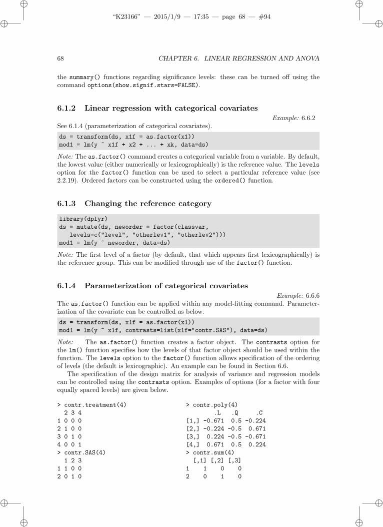
The AIC criterion also suggests that the model without the interaction is most appropriate.It may be useful to change the default reference level for variables. The default R design

matrix (see 6.1.4) can be changed and the model re-fit.

> contrasts(ds$sub) = contr.SAS(3)> aov3 = lm(cesd ~ sub + genf, data=ds)> summary(aov3)

Call:lm(formula = cesd ~ sub + genf, data = ds)

Residuals:Min 1Q Median 3Q Max

-32.13 -8.85 1.09 8.48 27.09

Coefficients:Estimate Std. Error t value Pr(>|t|)

(Intercept) 33.52 1.38 24.22 < 2e-16sub1 5.61 1.46 3.83 0.00014sub2 5.32 1.34 3.98 8.1e-05genfM -5.62 1.34 -4.20 3.3e-05

Residual standard error: 12.1 on 449 degrees of freedomMultiple R-squared: 0.0745,Adjusted R-squared: 0.0683F-statistic: 12 on 3 and 449 DF, p-value: 1.35e-07

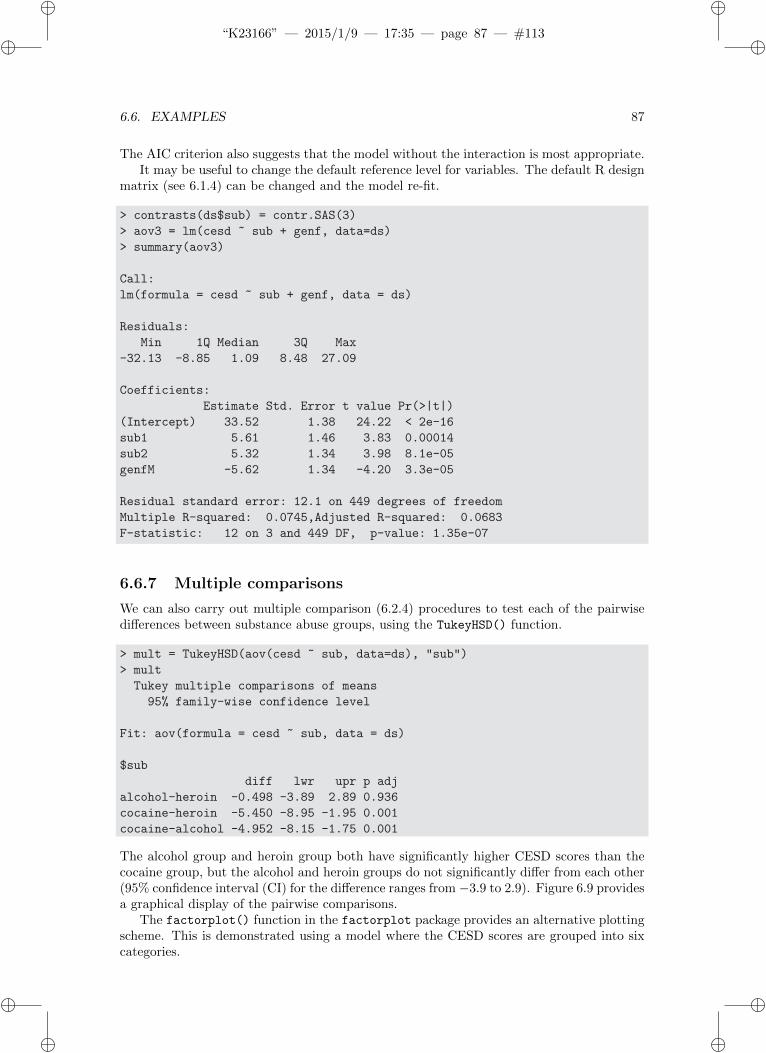
6.6.7 Multiple comparisons

We can also carry out multiple comparison (6.2.4) procedures to test each of the pairwisedi↵erences between substance abuse groups, using the TukeyHSD() function.

> mult = TukeyHSD(aov(cesd ~ sub, data=ds), "sub")> multTukey multiple comparisons of means95% family-wise confidence level

Fit: aov(formula = cesd ~ sub, data = ds)

$subdiff lwr upr p adj

alcohol-heroin -0.498 -3.89 2.89 0.936cocaine-heroin -5.450 -8.95 -1.95 0.001cocaine-alcohol -4.952 -8.15 -1.75 0.001

The alcohol group and heroin group both have significantly higher CESD scores than thecocaine group, but the alcohol and heroin groups do not significantly di↵er from each other(95% confidence interval (CI) for the di↵erence ranges from �3.9 to 2.9). Figure 6.9 providesa graphical display of the pairwise comparisons.

The factorplot() function in the factorplot package provides an alternative plottingscheme. This is demonstrated using a model where the CESD scores are grouped into sixcategories.

ii

“K23166” — 2015/1/9 — 17:35 — page 88 — #114 ii

ii

ii

88 CHAPTER 6. LINEAR REGRESSION AND ANOVA

> require(mosaic)> mplot(mult)

Tukey's Honest Significant Differences

difference in means

alcohol−heroin

cocaine−alcohol

cocaine−heroin

−8 −6 −4 −2 0 2

●

●

●

sub

Figure 6.9: Pairwise comparisons (using Tukey HSD procedure)

> library(dplyr)> library(factorplot)> newds = mutate(newds, cesdgrp = cut(cesd,

breaks=c(-1, 10, 20, 30, 40, 50, 61),labels=c("0-10", "11-20", "21-30", "31-40", "41-50", "51-60")))

> tally(~ cesdgrp, data=newds)

0-10 11-20 21-30 31-40 41-50 51-604 10 18 31 24 20

> mod = lm(pcs ~ age + cesdgrp, data=newds)> fp = factorplot(mod, adjust.method="none", factor.variable="cesdgrp",

pval=0.05, two.sided=TRUE, order="natural")

Figure 6.10 provides a graphical display of the fifteen pairwise comparisons, where thepairwise di↵erence is displayed above the standard error of that di↵erence (in italics).

6.6.8 Contrasts

We can also fit contrasts (6.2.3) to test hypotheses involving multiple parameters. In thiscase, we can compare the CESD scores for the alcohol and heroin groups to the cocainegroup.

ii

“K23166” — 2015/1/9 — 17:35 — page 89 — #115 ii

ii

ii

6.6. EXAMPLES 89

> plot(fp, abbrev.char=100)

11−2

0

21−3

0

31−4

0

41−5

0

51−6

0

41−50

31−40

21−30

11−20

0−10 1.745.53

6.395.17

9.684.97

8.005.05

14.795.12

4.653.69

7.953.40

6.263.52

13.053.62

3.302.78

1.612.91

8.403.04

−1.692.54

5.112.68

6.802.83

Significantly < 0Not SignificantSignificantly > 0

bold = brow − bcolital = SE(brow − bcol)

Figure 6.10: Pairwise comparisons (using the factorplot function)

> library(gmodels)> levels(ds$sub)[1] "heroin" "alcohol" "cocaine"> fit.contrast(aov2, "sub", c(1,1,-2), conf.int=0.95 )

Estimate Std. Error t value Pr(>|t|) lower CI upper CIsub c=( 1 1 -2 ) 10.9 2.42 4.52 8.04e-06 6.17 15.7

As expected from the interaction plot (Figure 6.7), there is a statistically significant di↵er-ence in this 1-degree-of-freedom comparison (p < 0.0001).