Embed Size (px)
Citation preview
Linear ProgrammingLinear Programming
OPIM 310-Lecture 2
Instructor: Jose Cruz

Model consisting of linear relationships Model consisting of linear relationships representing a firm’s objectives & resource representing a firm’s objectives & resource constraintsconstraints
Decision variables are mathematical Decision variables are mathematical symbols representing levels of activity of symbols representing levels of activity of an operationan operation
Objective function is a linear relationship Objective function is a linear relationship reflecting objective of an operationreflecting objective of an operation
Constraint is a linear Constraint is a linear relationship representing relationship representing a restriction on decision makinga restriction on decision making
Linear ProgrammingLinear Programming
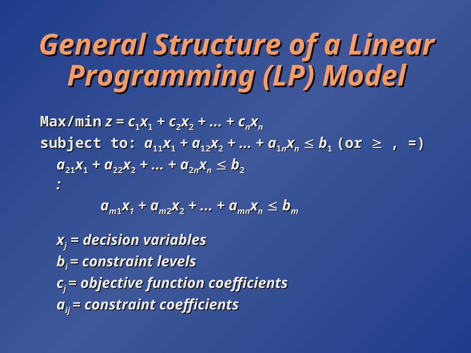
General Structure of a Linear General Structure of a Linear Programming (LP) ModelProgramming (LP) Model
Max/minMax/min z = c z = c11xx11 + c + c22xx22 + ... + c + ... + cnnxxnn
subject to:subject to: aa1111xx11 + a + a1212xx22 + ... + a + ... + a11nnxxnn bb11 (or(or , =), =)
aa2121xx11 + a + a2222xx22 + ... + a + ... + a22nnxxnn bb22
::
aamm11xx11 + a + amm22xx22 + ... + a + ... + amnmnxxnn bbmm
xxjj = decision variables = decision variables
bbi i = constraint levels= constraint levels
ccj j = objective function coefficients= objective function coefficients
aaij ij = constraint coefficients= constraint coefficients

Linear Programming Linear Programming Model FormulationModel Formulation
LaborLabor ClayClay RevenueRevenuePRODUCTPRODUCT (hr/unit)(hr/unit) (lb/unit)(lb/unit) ($/unit)($/unit)
BowlBowl 11 44 4040
MugMug 22 33 5050
There are 40 hours of labor and 120 pounds of clay There are 40 hours of labor and 120 pounds of clay available each dayavailable each day
Decision variablesDecision variables
xx11 = number of bowls to produce = number of bowls to produce
xx22 = number of mugs to produce = number of mugs to produce
RESOURCE REQUIREMENTSRESOURCE REQUIREMENTS
Example S9.1Example S9.1
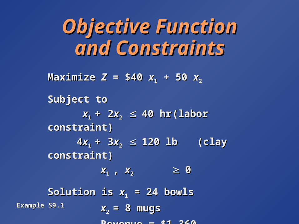
Objective Function Objective Function and Constraintsand Constraints
Maximize Maximize ZZ = $40 = $40 xx11 + 50 + 50 xx22
Subject toSubject to
xx11 ++ 22xx22 40 hr40 hr (labor constraint)(labor constraint)
44xx11 ++ 33xx22 120 lb120 lb (clay constraint)(clay constraint)
xx1 1 , , xx22 00
Solution is Solution is xx11 = 24 bowls = 24 bowls
xx2 2 = 8 mugs= 8 mugs
Revenue = $1,360Revenue = $1,360Example S9.1Example S9.1
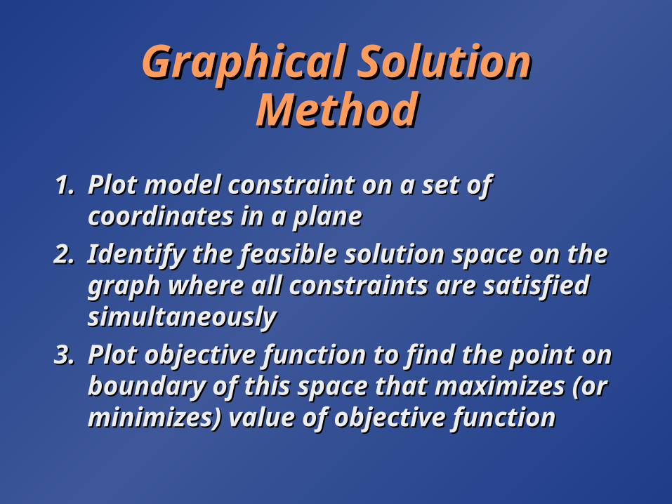
Graphical Solution Graphical Solution MethodMethod
1.1. Plot model constraint on a set of Plot model constraint on a set of coordinates in a planecoordinates in a plane
2.2. Identify the feasible solution space on the Identify the feasible solution space on the graph where all constraints are satisfied graph where all constraints are satisfied simultaneouslysimultaneously
3.3. Plot objective function to find the point on Plot objective function to find the point on boundary of this space that maximizes (or boundary of this space that maximizes (or minimizes) value of objective functionminimizes) value of objective function
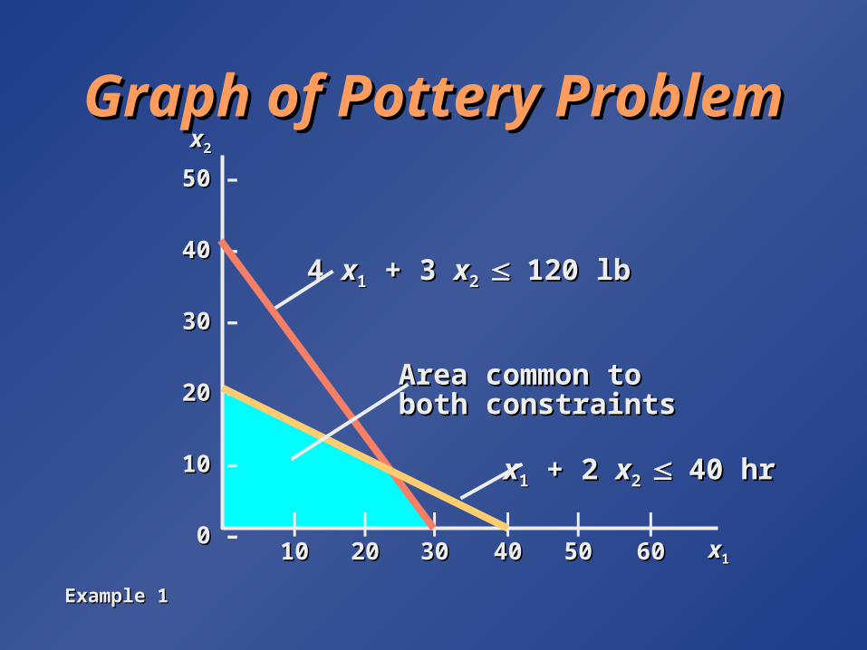
Graph of Pottery ProblemGraph of Pottery Problem
4 4 xx11 + 3 + 3 xx2 2 120 lb120 lb
xx11 + 2 + 2 xx2 2 40 hr40 hr
Area common toArea common toboth constraintsboth constraints
50 50 –
40 40 –
30 30 –
20 20 –
10 10 –
0 0 – |1010
|6060
|5050
|2020
|3030
|4040 xx11
xx22
Example 1Example 1
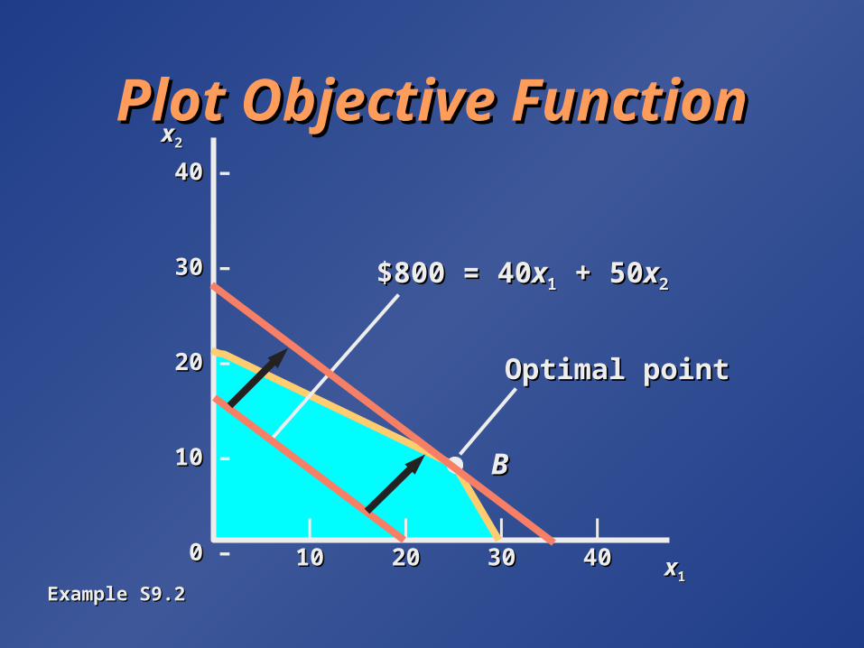
Plot Objective FunctionPlot Objective Function40 40 –
30 30 –
20 20 –
10 10 –
0 0 –
$800 = 40$800 = 40xx11 + 50 + 50xx22
Optimal pointOptimal point
BB
|1010
|2020
|3030
|4040 xx11
xx22
Example S9.2Example S9.2
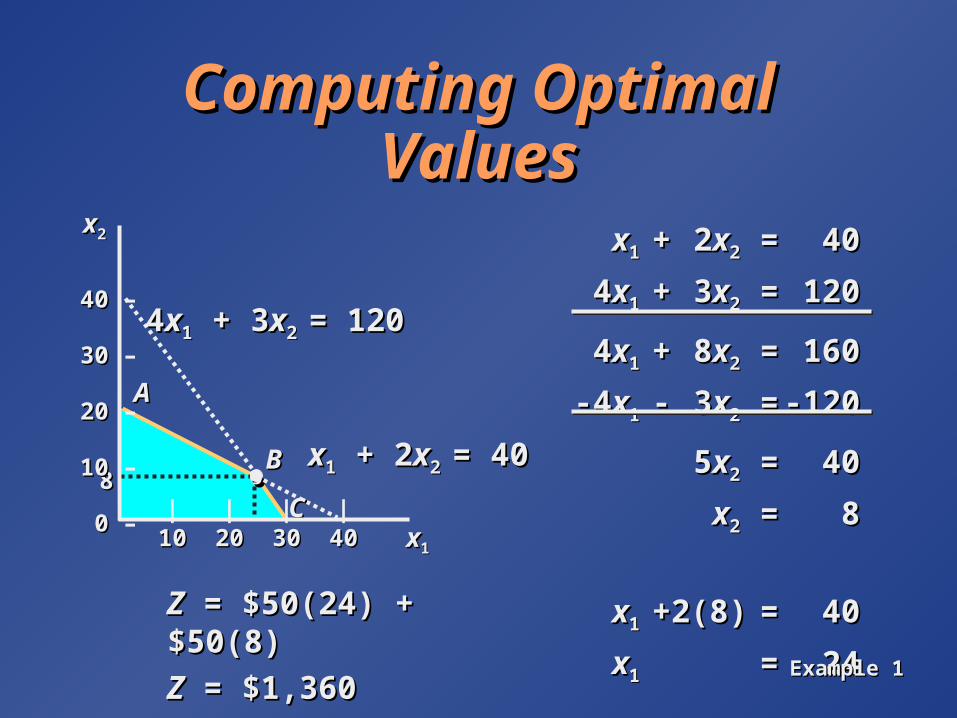
Computing Optimal Computing Optimal ValuesValues
ZZ = $50(24) + $50(8) = $50(24) + $50(8)
ZZ = $1,360 = $1,360
xx11 ++ 22xx22 == 4040
44xx11 ++ 33xx22 == 120120
44xx11 ++ 88xx22 == 160160
-4-4xx11 -- 33xx22 == -120-120
55xx22 == 4040
xx22 == 88
xx11 ++ 2(8)2(8) == 4040
xx11 == 2424
AA
..88BB
CC
xx11 + 2 + 2xx2 2 = 40= 40
44xx11 + 3 + 3xx2 2 = 120= 120
|2020
|3030
|4040
|1010 xx11
xx22
40 40 –
30 30 –
20 20 –
10 10 –
0 0 –
Example 1Example 1
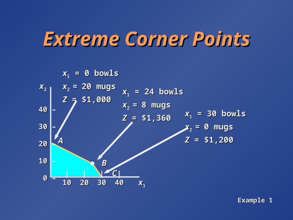
Extreme Corner PointsExtreme Corner Points
xx11 = 24 bowls = 24 bowls
xx2 2 ==8 mugs8 mugs
ZZ = $1,360 = $1,360 xx11 = 30 bowls = 30 bowls
xx2 2 ==0 mugs0 mugs
ZZ = $1,200 = $1,200
xx11 = 0 bowls = 0 bowls
xx2 2 ==20 mugs20 mugs
ZZ = $1,000 = $1,000
AA
BBCC|
2020|
3030|
4040|
1010 xx11
xx22
40 40 –
30 30 –
20 20 –
10 10 –
0 0 –
Example 1Example 1
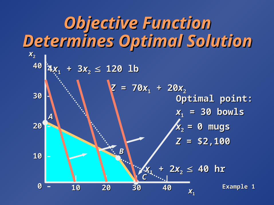
Objective Function Objective Function Determines Optimal SolutionDetermines Optimal Solution
44xx11 + 3 + 3xx2 2 120 lb120 lb
xx11 + 2 + 2xx2 2 40 hr40 hr
40 40 –
30 30 –
20 20 –
10 10 –
0 0 –
BB
|1010
|2020
|3030
|4040 xx11
xx22
CC
AA
ZZ = 70 = 70xx11 + 20 + 20xx22
Optimal point:Optimal point:
xx11 = 30 bowls = 30 bowls
xx2 2 ==0 mugs0 mugs
ZZ = $2,100 = $2,100
Example 1Example 1
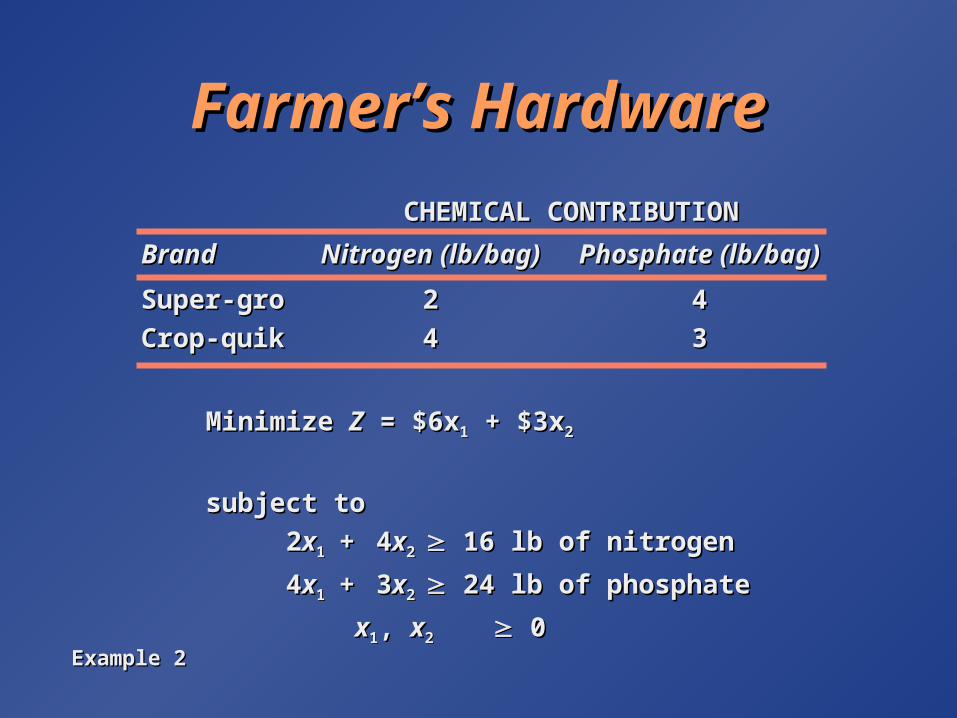
Farmer’s HardwareFarmer’s Hardware
CHEMICAL CONTRIBUTIONCHEMICAL CONTRIBUTION
BrandBrand Nitrogen (lb/bag)Nitrogen (lb/bag) Phosphate (lb/bag)Phosphate (lb/bag)
Super-groSuper-gro 22 44
Crop-quikCrop-quik 44 33
Minimize Minimize ZZ = $6x = $6x11 + $3x + $3x22
subject tosubject to
22xx11 ++ 44xx22 16 lb of nitrogen 16 lb of nitrogen
44xx11 ++ 33xx22 24 lb of phosphate 24 lb of phosphate
xx11, , xx22 0 0Example 2Example 2
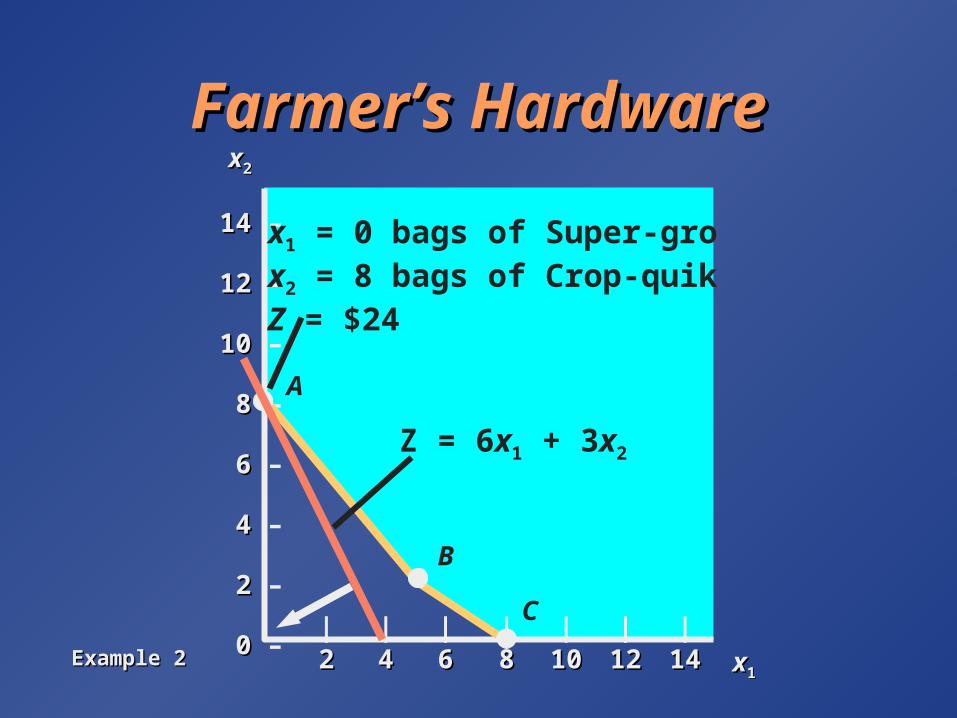
Farmer’s HardwareFarmer’s Hardware
14 14 –
12 12 –
10 10 –
8 8 –
6 6 –
4 4 –
2 2 –
0 0 –|22
|44
|66
|88
|1010
|1212
|1414 xx11
xx22
A
B
C
Z = 6x1 + 3x2
x1 = 0 bags of Super-grox2 = 8 bags of Crop-quikZ = $24
Example 2Example 2
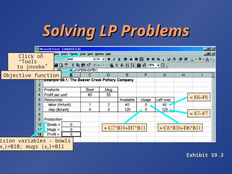
Solving LP ProblemsSolving LP Problems
Exhibit S9.3Exhibit S9.3
Click on “Tools” to invoke “Solver.”
Objective function
Decision variables – bowls(x1)=B10; mugs (x2)=B11

Solving LP ProblemsSolving LP Problems
Exhibit S9.4Exhibit S9.4
After all parameters and constraints have been input, click on “Solve.”
Objective function
Decision variables
C6*B10+D6*B11≤40
C7*B10+D7*B11≤120
Click on “Add” to insert contraints.
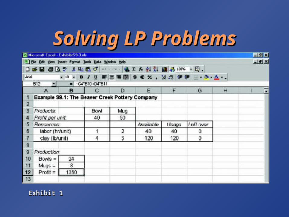
Solving LP ProblemsSolving LP Problems
Exhibit 1Exhibit 1
Example 2: Olympic Bike CoExample 2: Olympic Bike Co..
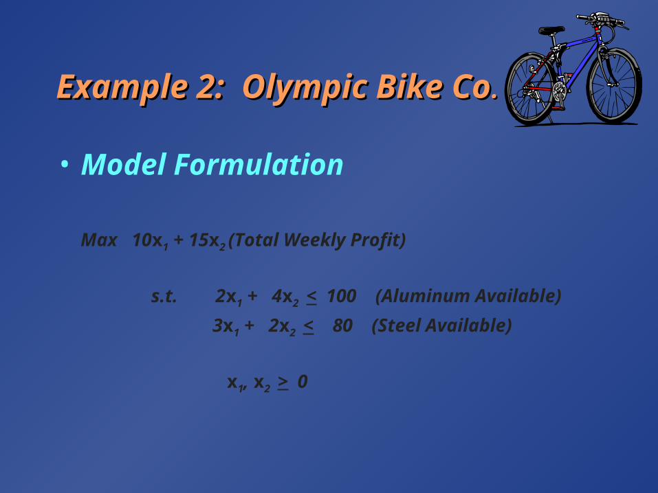
• Model Formulation
Max 10x1 + 15x2 (Total Weekly Profit)
s.t. 2x1 + 4x2 < 100 (Aluminum Available)
3x1 + 2x2 < 80 (Steel Available)
x1, x2 > 0

Example 2: Olympic Bike CoExample 2: Olympic Bike Co..
• Partial Spreadsheet Showing SolutionA B C D67 Deluxe Professional8 Bikes Made 15 17.5009
10 412.5001112 Constraints Amount Used Amount Avail.13 Aluminum 100 <= 10014 Steel 80 <= 80
Decision Variables
Maximized Total Profit
A B C D67 Deluxe Professional8 Bikes Made 15 17.5009
10 412.5001112 Constraints Amount Used Amount Avail.13 Aluminum 100 <= 10014 Steel 80 <= 80
Decision Variables
Maximized Total Profit

Example 2: Olympic Bike Co.Example 2: Olympic Bike Co.
• Optimal Solution
According to the output:
x1 (Deluxe frames) = 15
x2 (Professional frames) = 17.5
Objective function value = $412.50

Example 2: Olympic Bike Co.Example 2: Olympic Bike Co.
• Range of Optimality
Question
Suppose the profit on deluxe frames is increased to $20. Is the above solution still optimal? What is the value of the objective function when this unit profit is increased to $20?
Example 2: Olympic Bike CoExample 2: Olympic Bike Co..
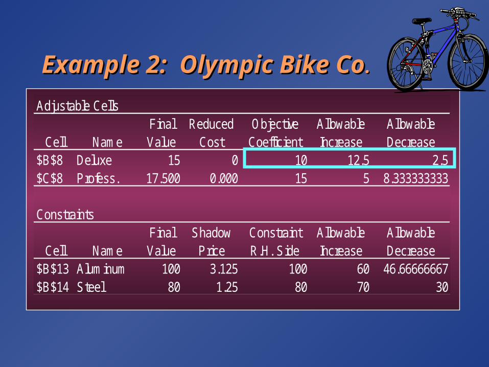
• Sensitivity Report Adjustable Cells
Final Reduced Objective Allowable AllowableCell Name Value Cost Coefficient Increase Decrease
$B$8 Deluxe 15 0 10 12.5 2.5$C$8 Profess. 17.500 0.000 15 5 8.333333333
ConstraintsFinal Shadow Constraint Allowable Allowable
Cell Name Value Price R.H. Side Increase Decrease$B$13 Aluminum 100 3.125 100 60 46.66666667$B$14 Steel 80 1.25 80 70 30
Example 2: Olympic Bike Co.Example 2: Olympic Bike Co.
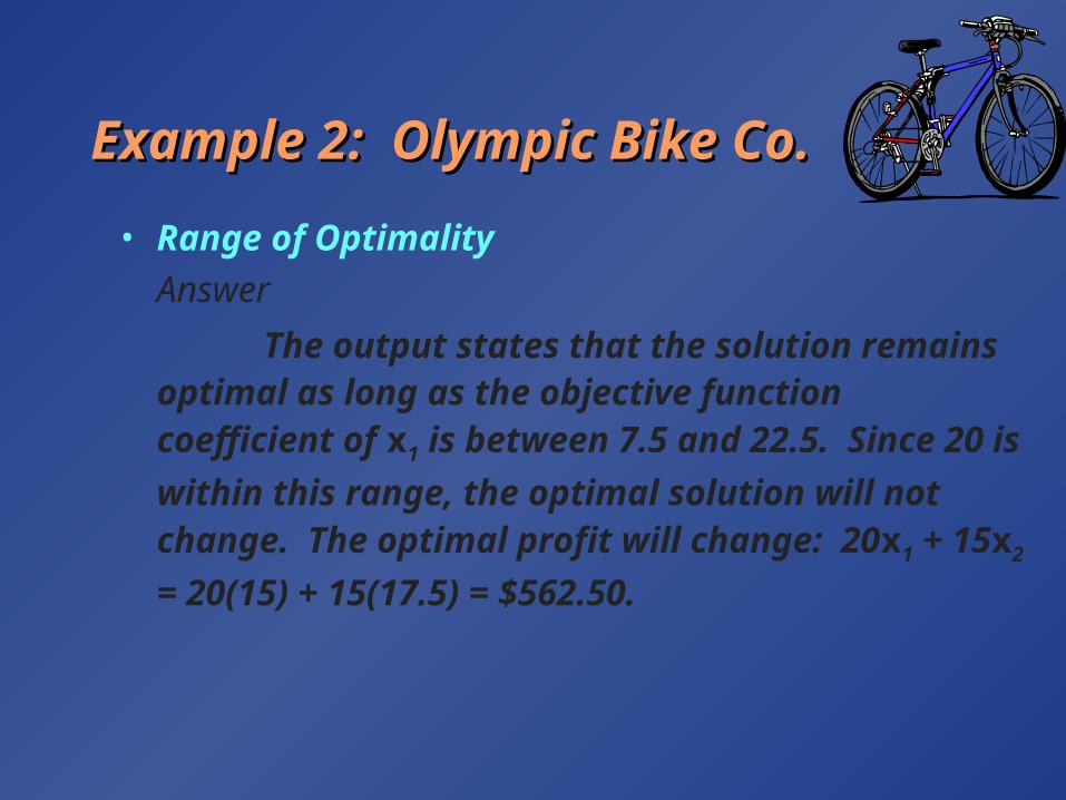
• Range of Optimality
Answer
The output states that the solution remains optimal as long as the objective function coefficient of x1 is between 7.5 and 22.5. Since 20
is within this range, the optimal solution will not change. The optimal profit will change: 20x1 +
15x2 = 20(15) + 15(17.5) = $562.50.

Example 2: Olympic Bike Co.Example 2: Olympic Bike Co.
• Range of Optimality
Question
If the unit profit on deluxe frames were $6 instead of $10, would the optimal solution change?

Example 2: Olympic Bike Co.Example 2: Olympic Bike Co.
• Range of Optimality Adjustable Cells
Final Reduced Objective Allowable AllowableCell Name Value Cost Coefficient Increase Decrease
$B$8 Deluxe 15 0 10 12.5 2.5$C$8 Profess. 17.500 0.000 15 5 8.33333333
ConstraintsFinal Shadow Constraint Allowable Allowable
Cell Name Value Price R.H. Side Increase Decrease$B$13 Aluminum 100 3.125 100 60 46.66666667$B$14 Steel 80 1.25 80 70 30
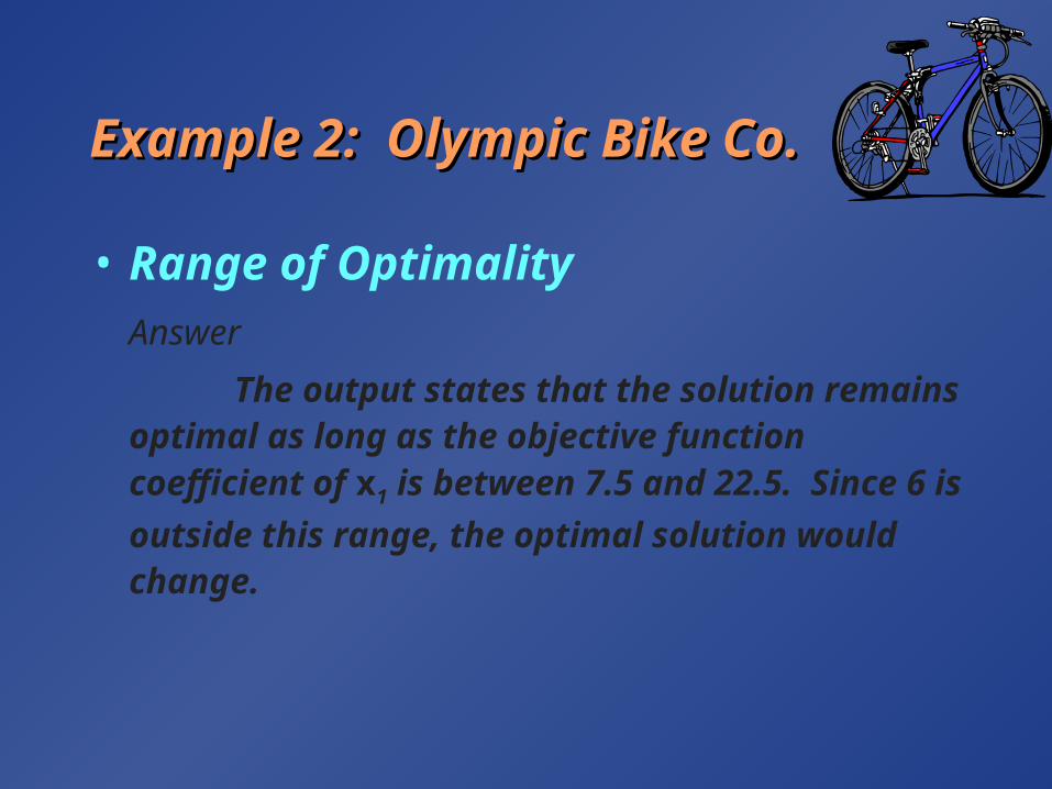
• Range of OptimalityAnswer
The output states that the solution remains optimal as long as the objective function coefficient of x1 is between 7.5 and 22.5. Since 6
is outside this range, the optimal solution would change.
Example 2: Olympic Bike Co.Example 2: Olympic Bike Co.

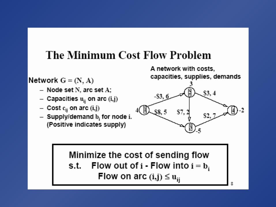
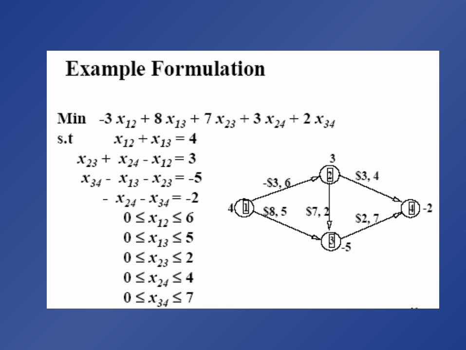
The Minimum Cost Network The Minimum Cost Network Flow Problem (MCNFP)Flow Problem (MCNFP)
• Extremely Useful Model in OR & EM• Important Special Cases of the MCNFP
– Transportation and Assignment Problems– Maximum Flow Problem– Minimum Cut Problem– Shortest Path Problem
• Network Structure– Some MCNFP LP’s have integer values !!!– Problems can be formulated graphically


Formulation of Shortest Path Formulation of Shortest Path ProblemsProblems
• Source node s has a supply of 1• Sink node t has a demand of 1• All other nodes are transshipment nodes• Each arc has capacity 1 • Tracing the unit of flow from s to t gives a
path from s to t
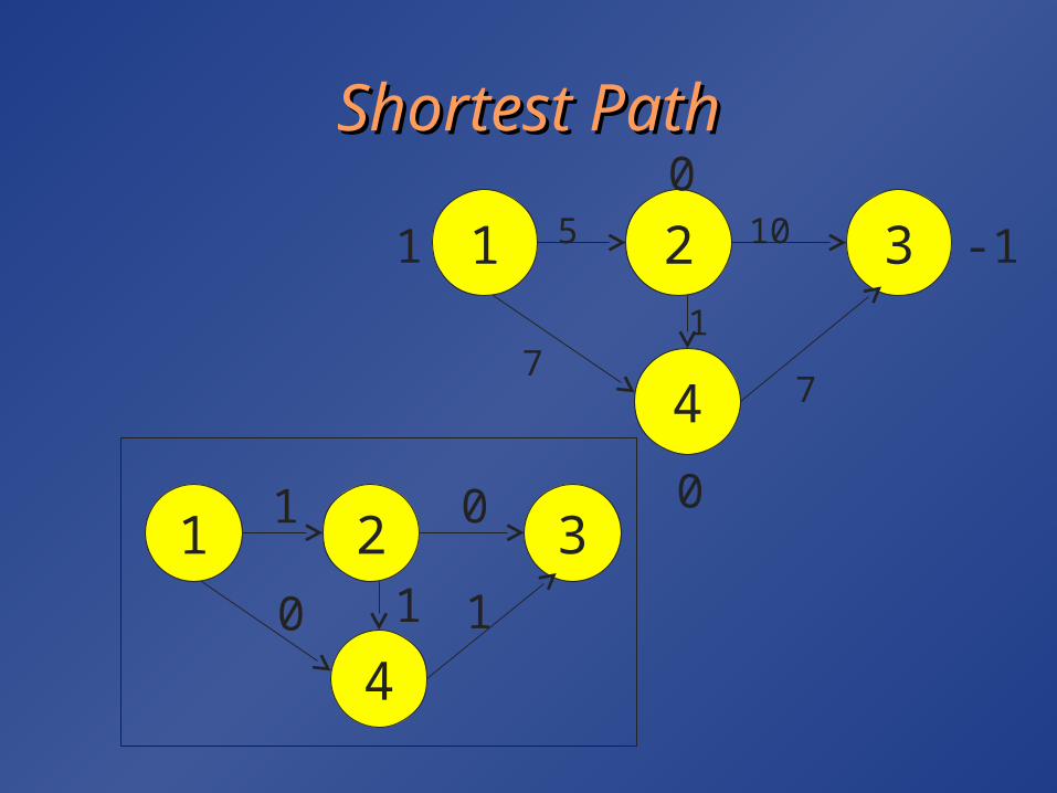
Shortest PathShortest Path
1 -11 2 3
4
5 10
11 2 3
4
1 0
10
0
0
77
1

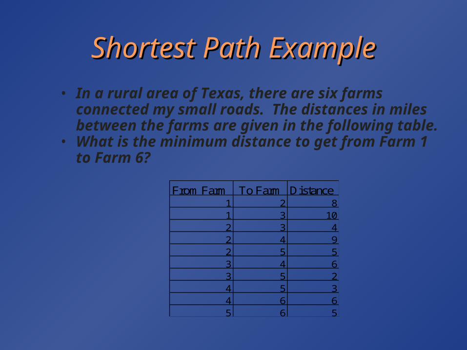
Shortest Path ExampleShortest Path Example• In a rural area of Texas, there are six farms
connected my small roads. The distances in miles between the farms are given in the following table.
• What is the minimum distance to get from Farm 1 to Farm 6?
From Farm To Farm Distance 1 2 81 3 102 3 42 4 92 5 53 4 63 5 24 5 34 6 65 6 5

Formulation as Shortest PathFormulation as Shortest Path
s t
1
2 4
3
9
10
56
6
8 45
5
4
2
3
1 -1
0 0
00

LP FormulationLP Formulation
10
1
0
0
0
0
1st
min
5646
45352556
34244546
23133534
12252423
1312
5646453534
2524231312
54326594108
xxx
xxxxxxxxxxxxxxxx
xxxxxxxxxxxx
ij