MASSACHUSETTS INSTITUTE OF TECHNOLOGYDEPARTMENT OF MECHANICAL ENGINEERING

2.151 Advanced System Dynamics and Control

Linear Graph Modeling: One-Port Elements1

1 Introduction

In the previous handout Energy and Power Flow in State Determined Systems we examined elemen-tary physical phenomena in five separate energy domains and used concepts of energy flow, storageand dissipation to define a set of lumped elements. These primitive elements form a set of buildingblocks for system modeling and analysis, and are known generically as lumped one-port elements,because they represent the spatial locations (ports) in a system at which energy is transferred. Foreach of the domains with the exception of thermal systems, we defined three passive elements, twoof which store energy and a third dissipative element. In addition in each domain we defined twoactive source elements which are time varying sources of energy.

System dynamics provides a unified framework for characterizing the dynamic behavior of sys-tems of interconnected one-port elements in the different energy domains, as well as in non-energeticsystems. In this handout the one-port element descriptions are integrated into a common descrip-tion by recognizing similarities between the elemental behavior in the energy domains, and bydefining analogies between elements and variables in the various domains. The formulation ofa unified framework for the description of elements in the energy domains provides a basis fordevelopment of unified methods of modeling systems which span several energy domains.

The development of a unified modeling methodology requires us to draw analogies betweenthe variables and elements in different energy domains. Several different types of analogs may bedefined. In this text we have chosen to relate elements using the concepts of generalized “through”and “across” variables associated with a linear graph system representation introduced by F.A.Firestone [1] and H.M. Trent [2], and described in detail in several texts [3-5]. This set of analogsallows us to develop modeling methods that are similar to well known techniques for electricalcircuit analysis. The set of analogies we have selected is not unique, for example another widelyused analogy is based on the concepts of “effort” and “flow” variables in bond graph modelingmethods, developed by H.M. Paynter [6] and described in D.C. Karnopp, et al. [7]. These twomethods lead to different analogies both of which are valid. For example, in this text we considerforces and electrical currents to be analogous, while in the bond graph method forces and electricalvoltages are considered to be similar.

2 Generalized Through and Across Variables

Figure 1 shows a schematic representation of a single one-port element, in this case a mechanicalspring, as a generic element with two “terminals” through which power flows, either to be stored,supplied, or dissipated by the element. This two-terminal representation may be thought of as amechanical analog of an electrical element, in this case an inductor, with two connecting “wires”. Ifall system elements are represented in this form, the interconnection of elements may be expressedin a common “circuit” structure and a unified method of modeling and analysis may be derived

1D. Rowell - Revised: 9/16/04

1

F(t)

F(t)

v (t)

v (t)

1

2

1

2

(c)

1

2

Power flow

1

2

node

branch v (t)

1 v (t)

2

(b) (a)

Figure 1: Schematic representation of a typical one-port element (a) a translational spring, (b) asa two-terminal element, and (c) as a linear graph element.

for this form known as a linear graph. In Fig. 1(c) the linear graph representation of the springelement is shown as a branch connecting two nodes.

With the two-terminal representation, one of the two variables associated with the element is aphysical quantity which may be considered to be measured “across” the terminals of the element,and the other variable represents a physical quantity which passes “through” the element. Forexample, in the case of mechanical elements such as the spring in Fig. 1 the two defined variablesare v, the velocity, and F , the force associated with the element. The velocity associated with amechanical element is defined to be the differential (or relative) velocity as measured between thetwo terminals of the element, that is v = v2 − v1 in Fig. 1; notice that it must be measured acrossthe element. Figure 2 shows a simple system with the same spring connected between a mass mand an applied force source F (t). In Fig. 2b the connection has been broken so that the forcesacting on the spring and the mass may be examined. Assume that the force transmitted to themass is Fm(t). Because the spring element is assumed to be massless, Newton’s laws of motionrequire that the sum of all external forces acting on it must sum to zero, or

F (t)− Fm(t) = 0.

In other words Fm(t) = F (t), and the external force applied to the spring element is transmittedthrough the spring to the mass element connected to the other side. Another way of looking at thisis to say that in order to measure the force (tension) in a mechanical element, the element mustbe broken and a sensing device, such as a spring balance, inserted in series with the element as inFig. 2b. Such arguments lead us to define elemental velocity v to be an across-variable, and forceF to be a through-variable in mechanical systems.

Figure 3 shows a simple electrical circuit consisting of a battery and a resistor. The elementalvariables in the electrical domain are current i and voltage drop v. In order to measure the currentflowing in the resistor the electrical circuit must be broken, and an ammeter inserted so that thecurrent flows through it. To measure the voltage drop associated with the resistor a voltmeter isconnected directly across its terminals. Current is defined as the through-variable for electricalsystems, and voltage drop is the across-variable.

We may extend the concept of through and across variables to all of the energy domains de-scribed in the handout Energy and Power Flow in State Determined Systems. Of the two variablesdefined for each domain, one is defined to be an across-variable because it is a relative quantity

2

v (t) 2 v (t) 1

F(t) m

K

v (t) 2

v (t) 1

F(t) m

K

F

(a) Mass and spring elements driven by an external force.

V

(b) Force is measured by inserting an instrument in series with the elements, velocity is measured by connecting an instrument across an element.

Figure 2: Definition of through and across variables in a simple mechanical system.

that must be measured as a difference between values at the two terminals of a network element.The other is designated as a through-variable that is continuous through any two-terminal element.Once the choice of this pair of variables has been established, generalized modeling and analysistechniques may be developed without regard to the particular energy domains associated with asystem.

The through and across-variables for each energy domain discussed in this book are definedbelow:

Mechanical Systems: In both translational and rotational mechanical systems thevelocity drop of an element is the velocity difference across its terminals. In the case ofa translational mass or rotary inertia one terminal is always assumed to be connectedto a constant velocity inertial reference frame. The force or torque associated with

V

A

R

i

v R

+

-

An ammeter measures current "through" an element.

A voltmeter measures voltage "across" an element

V

Figure 3: Definition of through and across variables in an electrical system.

3

an element is assumed to pass through the element. The elemental across-variable istherefore defined to be the relative velocity of the two terminals, and the elementalthrough-variable is defined to be the force or torque associated with the element.Electrical Systems: In an electrical element, for example a capacitor, at any instant apotential (or voltage) difference exists between the terminals and a current flows throughthe element. The across-variable is therefore defined to be the voltage drop across theelement, and the through-variable is defined to be the current flowing through the ele-ment.Fluid Systems: In the fluid domain the pressure difference across an element satisfiesthe definition of an across-variable, while the volume flow rate through the element isa natural choice for the through-variable.Thermal Systems: While not strictly analogous to the other domains, thermal sys-tems may be analyzed by defining heat flow rate as the through-variable, and the tem-perature difference across an element as the across-variable.

The definitions of across and through-variables for all the energy domains are summarized in Ta-ble 1. In describing generic systems, without regard to a specific energy domain, it is convenient todefine a set of generalized variables. The generalized across and through-variables are introduced as:

Generalized across-variable: v

Generalized integrated across-variable: x =∫ t

0vdt + x(0)

Generalized through-variable: f

Generalized integrated through-variable: h =∫ t

0fdt + h(0)

With the exception of thermal elements, the power P passing into a lumped one-port elementin terms of the generalized variables is:

P = fv (1)

and the work performed by the system on the element over time period 0 ≤ t ≤ T may be expressedin terms of the generalized variables as:

W =∫ T

0Pdt =

∫ T

0fvdt. (2)

For thermal elements while an across-variable, temperature T , and a through variable, heatflow rate Q, may also be defined, the product is not power since Q is a power variable itself.

3 Generalization of One-Port Elements

In each of the energy domains, several primitive elements are defined: one or two ideal energystorage elements, a dissipative element, and a pair of source elements. For one of the energystorage elements, the energy is a function of its across-variable (for example an ideal mass elementstores energy as a function of its velocity; E = 1

2mv2), while in the other energy storage elementthe stored energy is a function of the through-variable; in a translational spring the stored energyis E = 1

2KF 2. The dissipative elements, which store no energy, and the source elements, whichmay supply energy or power continuously, complete the set of one-port elements. In this sectionthese elements are classified into generic groups.

4

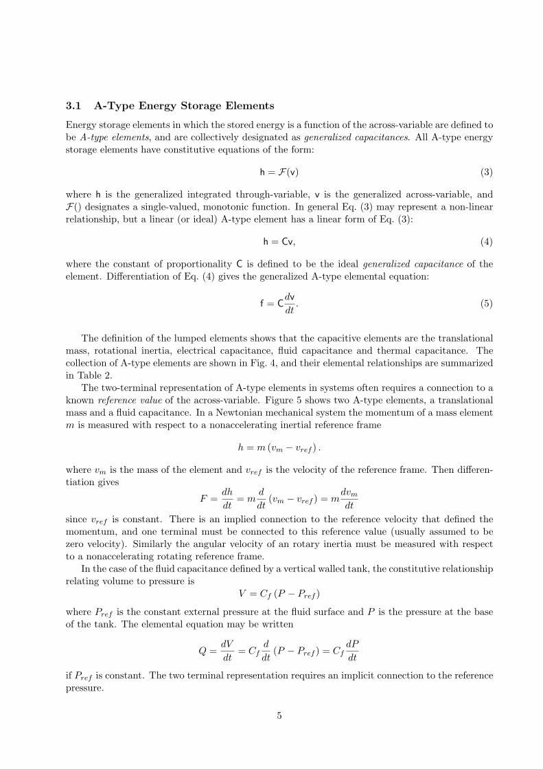
3.1 A-Type Energy Storage Elements

Energy storage elements in which the stored energy is a function of the across-variable are defined tobe A-type elements, and are collectively designated as generalized capacitances. All A-type energystorage elements have constitutive equations of the form:

h = F(v) (3)

where h is the generalized integrated through-variable, v is the generalized across-variable, andF() designates a single-valued, monotonic function. In general Eq. (3) may represent a non-linearrelationship, but a linear (or ideal) A-type element has a linear form of Eq. (3):

h = Cv, (4)

where the constant of proportionality C is defined to be the ideal generalized capacitance of theelement. Differentiation of Eq. (4) gives the generalized A-type elemental equation:

f = Cdv

dt. (5)

The definition of the lumped elements shows that the capacitive elements are the translationalmass, rotational inertia, electrical capacitance, fluid capacitance and thermal capacitance. Thecollection of A-type elements are shown in Fig. 4, and their elemental relationships are summarizedin Table 2.

The two-terminal representation of A-type elements in systems often requires a connection to aknown reference value of the across-variable. Figure 5 shows two A-type elements, a translationalmass and a fluid capacitance. In a Newtonian mechanical system the momentum of a mass elementm is measured with respect to a nonaccelerating inertial reference frame

h = m (vm − vref ) .

where vm is the mass of the element and vref is the velocity of the reference frame. Then differen-tiation gives

F =dh

dt= m

d

dt(vm − vref ) = m

dvm

dt

since vref is constant. There is an implied connection to the reference velocity that defined themomentum, and one terminal must be connected to this reference value (usually assumed to bezero velocity). Similarly the angular velocity of an rotary inertia must be measured with respectto a nonaccelerating rotating reference frame.

In the case of the fluid capacitance defined by a vertical walled tank, the constitutive relationshiprelating volume to pressure is

V = Cf (P − Pref )

where Pref is the constant external pressure at the fluid surface and P is the pressure at the baseof the tank. The elemental equation may be written

Q =dV

dt= Cf

d

dt(P − Pref ) = Cf

dP

dt

if Pref is constant. The two terminal representation requires an implicit connection to the referencepressure.

5

System Across-Variable (v) Through-Variable (f)

Translational velocity difference (v) force (F )Rotational angular velocity difference (Ω) torque (T )Electrical voltage drop (v) current (i)Fluid pressure difference (P ) volume flow rate (Q)Thermal temperature difference (T ) heat flow rate (q)

System Integrated Across-Variable (x) Integrated Through-Variable (h)

Translational linear displacement (x) momentum (p)Rotational angular displacement (Θ) angular momentum (h)Electrical flux linkage (λ) charge (q)Fluid pressure difference momentum (Γ) volume (V )Thermal (not defined) heat (H)

Table 1: Definition of across and through-variables in the various energy domains.

v

F m T

W r e f

W JC

iv 1

v 2( a ) T r a n s l a t i o n a l m a s s ( b ) R o t a t i o n a l i n e r t i a ( c ) E l e c t r i c a l c a p a c i t o r

v r e f

C t

T r e f

qT

( d ) F l u i d c a p a c i t a n c e ( e ) T h e r m a l c a p a c i t a n c e

C f PQ

P r e f

Figure 4: The A-type elements in the five energy domains described in this handout.

6

Element Constitutive equation Elemental equation Energy

Generalized A-type h = Cv f = Cdv

dtE =

12Cv2

Translational mass p = mv F = mdv

dtE =

12mv2

Rotational inertia h = JΩ T = JdΩdt

E =12JΩ2

Electrical capacitance q = Cv i = Cdv

dtE =

12Cv2

Fluid capacitance V = CfP Q = CfdP

dtE =

12CfP 2

Thermal capacitance H = CtT q = CtdT

dtE = CtT

Table 2: Summary of elemental relationships for ideal A-type elements.

F ( t )m

v

I n e r t i a l r e f e r e n c e f r a m e v r e fQ

hP = r g hr e l a t i v e t o P r e f

P r e f

( a ) ( b )

Figure 5: Implicit connection of typical A-type elements to a reference node, (a) a translationalmass, and (b) a fluid capacitance.

Similarly the temperature associated with a thermal capacitance is measured with respect toa fixed reference temperature. The electrical capacitor, however, does not require connection to afixed reference voltage and may have its two terminals connected to points of arbitrary voltage.

With the exception of the thermal capacitance, the energy stored in a pure or ideal A-typeelement is given by:

E =∫ h

0vdh. (6)

For an ideal element with a constitutive equation given by Eq. (6), the stored energy can beexpressed as:

E =∫ h

0

h

Cdh =

12

h2

C=

12Cv2 (7)

resulting in a form in which the energy is a direct function of the across-variable. For the idealthermal capacitance the energy is simply E = H = CtT and is a function of the across-variable.

7

óõ f d t1C_ vf

óõ f d t1C_ vf

f

ft

t

t

t

v

vC

v 1

v 2

f

( a ) G e n e r a l i z e d c a p a c i t a n c e ( b ) R e s p o n s e o f c a p a c i t a n c e t o d i s c o n t i n u o u s c h a n g e s i n t h e t h r o u g h v a r i a b l e .

Figure 6: Across and through-variable relationships in an ideal A-type element.

Example

Show that that an A-type element is capable of both absorbing and supplying power.

Solution: For an A-type element the instantaneous power flow is

P = fv = Cdv

dtv. (8)

Our sign convention is that if P > 0, power is flowing into the element, while if P < 0power is flowing from the element. Thus the direction of power flow is defined by Eq.(i); if v and dv/dt have the same sign the element is absorbing power and storing energy,while if the signs are opposite the element is returning stored energy to the system.

Consider a mechanical mass element. Equation (i) states that the element is accumu-lating energy whenever it is accelerated in the direction of its travel, and returns energyas it is decelerated.

Equation (7) shows that any change in the stored energy in an A-type element results froma change in the across-variable. In order to change the energy in a step-wise fashion the across-variable must change instantaneously. Eq. (5) shows that the through-variable is proportionalto the derivative of the across-variable, therefore an instantaneous change in the stored energyrequires an impulse in the through-variable. The stored energy in any A-type element cannotchange instantaneously unless infinite power is available in the form of an impulse in force, torque,current or volume flow. Physical energy sources are generally power limited, and are thereforeincapable of providing an instantaneous change in the across-variable or stored energy of an A-type element. Fig. 6 shows the relationships between across and through-variables for an A-typeelement.

Example

A satellite circling the earth every 90 minutes is subjected to cyclic heating by the sunas it passes in and out of the earth’s shadow. Measurements have shown that it isreasonable to model the net solar heat flow rate Q(t) into the satellite as a cosinusoidal

8

function with the orbital period, assuming that at time t = 0 the satellite is at theposition of peak sunlight. Find the time in the orbit at which the internal temperaturewithin the satellite is a maximum.

Solution: Let the time t be measured in seconds, so that the the heat flow rate is

Q(t) = Qmax cos(

2π

90× 60t

). (9)

where Qmax is the peak heat flow rate (joules/sec). The satellite is modeled as a lumpedthermal capacitance Ct and stores energy as an A-type thermal element. For a generalA-type element the elemental equation is

f = Cdv

dt, (10)

and for the thermal capacitance the relationship is

Q = CtdT

dt. (11)

In this case we require the value of T (t), given Q(t), so that Eq. (iii) must be writtenin integral form:

T (t) =1Ct

∫ t

0Qdt + T (0) (12)

=1Ct

∫ t

0Qmax cos

(2π

5400t

)dt + T (0) (13)

=5400Qmax

2πCtsin

(2π

5400t

)+ T (0) (14)

The system input Q(t) and the response T (t) are shown in Fig. 7. The temperature and

1000 2000 3000 4000 5000

-1

-0.5

0

0.5

1

t

q

Q max

_____

T - T(0)

T - T(0) max

_________

Time (secs)

Norm

aliz

ed h

eat flo

w

Norm

aliz

ed tem

pera

ture

Figure 7: The input heat flow rate Q(t) and the temperature response T (t) of the satellite.

the input heat flow are not in synchrony; the response lags the input by one quarter ofa cycle. Since sin θ is a maximum when θ = π/2, T (t) is a maximum when 2πt/5400 =π/2, or when t = 1350 sec. The satellite therefore reaches its maximum temperature 22.5minutes after passing the point of maximum brightness, and the maximum temperatureis:

Tmax =5400Qmax

2πCt+ T (0) (15)

9

FF

v v

12

12

T

TW

W 1

2 1

2

K rK

12

Lv v 12

I1

2

P

P

Q

f2

1

( a ) T r a n s l a t i o n a l s p r i n g ( b ) T o r s i o n a l s p r i n g

( c ) E l e c t r i c a l i n d u c t a n c e ( d ) F l u i d i n e r t a n c e

Q

i i

Figure 8: The T-type elements in the energy domains described in this handout. There is no T-typeelement for the thermal domain.

3.2 T-Type Energy Storage Elements

Energy storage elements in which the stored energy may be expressed as a function of the through-variable are designated as T-type elements, and are collectively known as generalized inductances.The T-type energy storage elements are defined by generalized constitutive equations of the form:

x = F(f) (16)

where x is the generalized integrated across-variable, f is the generalized through-variable, andF() designates a single-valued, monotonic function. For a linear, or ideal, T-type element theconstitutive relationship Eq. (16) reduces to a simple linear equation

x = Lf (17)

where the constant of proportionality L is defined to be the ideal generalized inductance. Differen-tiation of the constitutive equation gives the generalized elemental equation:

v = Ldf

dt. (18)

Figure 8 shows the four T-type elements; there is no known thermal energy storage phenomenonthat defines a T-type element for thermal systems. The generalized inductance is equivalent to thereciprocal of the mechanical translational and rotational spring constants, and is equivalent to theelectrical inductance and the fluid inertance. Table 3 summarizes the elemental relationships forT-type elements.

The energy stored in a T-type pure or ideal element is given by:

E =∫ x

0fdx (19)

For an ideal element, with a constitutive equation of Eq. (19), the energy is a direct functionof the through-variable f:

E =∫ x

0

x

Ldx =

12

x2

L=

12Lf2. (20)

10

Element Constitutive equation Elemental equation Energy

Generalized T-type x = Lf v = Ldf/dt E =12Lf2

Translational spring x =1K

F v =1K

dF

dtE =

12K

F 2

Torsional spring Θ =1

KrT Ω =

1Kr

dT

dtE =

12Kr

T 2

Electrical inductance λ = Li v = Ldi

dtE =

12Li2

Fluid inertance Γ = IfQ P = IfdQ

dtE =

12IfQ2

Table 3: Summary of elemental relationships for ideal T-type elements.

As in the case of an A-type element, it is not possible to change the stored energy or the through-variable in a T-type element instantaneously without an infinite source of power.

Example

It is commonly observed in electrical circuits containing inductances that when a switchis opened a brief electrical arc may develop across the air gap, causing the switchcontacts to become pitted. In severe cases arcing may occur between the turns of thecoil itself causing breakdown of the electrical insulation and perhaps destruction of theinductor. Explain why this arcing occurs.Solution: Consider the circuit shown in Fig. 9. An inductor is a T-type element, and

R

+

-

V L

Figure 9: An electrical circuit containing an inductance.

has an elemental equation

v = Ldi

dt. (21)

If a current i is flowing just before the switch is opened, the energy stored in the magneticfield of the inductor is E = 1

2Li2. When the current is interrupted the magnetic field“collapses” and the stored energy must be either returned to the system or dissipated.The rapid change in the magnetic flux as the field decays generates a large inductive

11

voltage in the coil. This induced voltage is sufficient to cause the arc, a short currentpulse across the gap, that is potentially damaging to the switch and the coil itself. Theinductive back emf (electromotive force) attempts to maintain the current through thecoil so as to dissipate the stored energy.

This phenomenon may be described in terms of the elemental equation Eq. (i). Anattempt to decrease the current instantaneously creates a large negative value of thederivative di/dt, generating a correspondingly large value of the across-variable v. Thearcing allows the current to continue briefly after the switch is opened and thereforeto decay in a finite time. In practice engineers often connect semiconductor diodes orcapacitors across inductors to provide an alternate current path and reduce inductivevoltage spikes and arcing.

3.3 D-Type Dissipative Elements

The elements that dissipate energy are collectively known as D-type elements. They are defined byan algebraic relationship between the across and through-variables of the form:

v = F(f) or f = F−1(v) (22)

where f and v are the generalized through and across variables respectively. For linear (ideal)dissipative elements the relationship is commonly expressed in two forms:

v = Rf or f =1R

v (23)

where R is defined to be the generalized ideal resistance. It is also common to define the conductanceG = 1/R as the reciprocal of the resistance and to write Eqs. (23) as

f = Gv or v =1G

f. (24)

The generalized resistances are equivalent to the reciprocals of the mechanical and rotationaldamping constants, and are equivalent to the electrical, fluid and thermal resistances. For all D-type elements, except the thermal resistance element, power supplied to the element is convertedinto heat and dissipated. For the ideal elements the power may be expressed as:

P = Rf2 =1R

v2. (25)

The power P is always a positive quantity, and flows into a D-type element.In the thermal D-type element power is not dissipated. In this case, because the through-

variable is power, the element simply acts to impede heat flow. Table 4 summarizes the algebraicD-type relationships for resistances.

The dissipative elements store no energy and instantaneous changes in the power dissipatedby the elements are associated with instantaneous changes in the through and across-variables asindicated by the ideal elemental equation in which the through and across-variables are directlyrelated by the constant R.

12

Element Elemental equations Power dissipated

Generalized D-type f =1R

v v = Rf P =1R

v2 = Rf2

Translational damper F = Bv v =1B

F P = Bv2 =1B

F 2

Rotational damper T = BrΩ Ω =1

BrT P = BrΩ2 =

1Br

T 2

Electrical resistance i =1R

v v = Ri P =1R

v2 = Ri2

Fluid resistance Q =1

RfP P = RfQ P =

1Rf

p2 = Q2Rf

Thermal resistance q =1Rt

T T = Rtq

Table 4: Summary of elemental relationships for ideal D-type elements.

Example

An electrical resistance of value R is connected to a voltage source that supplies asinusoidal voltage of the form V (t) = Vm sin(ωt) , as shown in Fig. 10. Find the averagepower dissipated in the resistor over one period of the voltage input.

Solution: The sinusoidal applied voltage V (t) repeats itself with a period T = 2π/ω

-RV s i n w tm

VR_ _ m s i n w ti =

Figure 10: An electrical resistance.

seconds. The instantaneous power dissipated in the resistance is

P(t) =v2(t)R

=V 2

m

Rsin2(ωt). (26)

The average power dissipated over one period T is found by integrating the power overone period and dividing by the period:

Pavg =1T

∫ T

0P(t)dt =

2π

ω

∫ 2π/ω

0

V 2m

Rsin2(ωt)dt

=V 2

mω

2πR

(π

ω

)=

(Vm√

2

)2 1R

. (27)

This expression shows that the average power dissipated in R over one period of thesinusoidal voltage is the same as would be dissipated by a constant applied voltage ofvalue v = Vm/

√2 = 0.707Vm volts.

13

2

1

2

1

F (t) V (t) s s

-

(a) Through-variable source (b) Across-variable source

Figure 11: Idealized source elements.

3.4 Ideal Sources

In each energy domain two general types of idealized sources may be defined:

• the ideal Across-Variable Source in which the generalized across-variable is a specified functionof time f(t)

Vs(t) = f(t),

and is independent of the through-variable, and

• the ideal Through-Variable Source in which the generalized through-variable is a specifiedfunction of time

Fs(t) = f(t)

and is independent of the across-variable.

An example of an through-variable source is an idealized positive displacement pump in a fluidsystem, in which the flow rate is a prescribed function of time and is independent of the pressurerequired to maintain the flow, while an example of an across-variable source is a regulated laboratoryelectrical power supply in which the output voltage is independent of the current drawn by thecircuit to which it is connected. The ideal sources are not power or energy limited and theoreticallymay supply infinite power and energy.

The symbols for the ideal sources are shown in Fig. 11 where in the through-variable source thearrow designates the assumed positive direction of through-variable flow, and in the across-variablesource the arrow designates the assumed direction of the across-variable decrease or drop. For eachsource type one variable is an independently specified function of time.

The value of the complementary variable of each source is determined by the system to whichthe source is connected. A source may provide power and energy to a system, or may absorb powerand energy, depending upon the sign of the complementary source variable. Table 5 defines thesource types in each of the energy domains.

Example

A force source is used to accelerate and deaccelerate a mass in a cyclic motion as shown

14

Energy Domain Across-variable source Through-variable source

Generalized Across-Variable Vs(t) Through variable Fs(t)

Mechanical translational Velocity source Vs(t) force source Fs(t)

Mechanical rotational Angular velocity source Ωs(t) Torque source Ts(t)

Electrical Voltage source Vs(t) current source Is(t)

Fluid Pressure source Ps(t) Flow source Qs(t)

Thermal Temperature source Ts(t) Heat flow source Qs(t)

Table 5: Definition of ideal sources.

m

v

F

v r e f

t

t

t

T

F

v

T

T

F

- F

v

- v

o

oo

o

o

oPF vo o

o- F vo o

F o r c e

V e l o c i t y

P o w e r

( i n p u t )

( r e s p o n s e )

Figure 12: A mass element driven by a force source.

in Fig. 12.The force source provides a square wave in force cycling between values of +Fo and−Fo with a total cycle time of To. In this example the velocity of the mass as a functionof time and the power flow into the mass as a function of time are to be determined.As shown in Fig. 12, the mass velocity is defined as positive when the force is positive.The velocity of the mass m is determined from the elemental equation

Fs = mdv

dt(28)

The problem solution may be found by solving Eq. (i) in each fraction of the total time.Over the time period 0 ≤ t < To/4, the elemental equation may be expressed as:

Fodt = mdv (29)

and integrated to yield:

v =1m

Fot (30)

15

Over the period To/4 ≤ t < 3To/4, the equation may also be integrated, noting that attime t = To/4 the mass has velocity vo to yield:

(−Fo)dt = mdv (31)

and integrated to yield:

v(t) = vo − Fo

m(t− To/4) (32)

Over the period of time 3To/4 ≤ t < To, the equation may be integrated, noting thatat time t = 3To/4, the velocity is −vo:

Fodt = mdv (33)

and integrated to yield:

v = −vo +Fo

m(t− 3To/4) (34)

Using the results from integration the elemental equation the velocity of the mass isplotted over one period of time To in Fig. 12. For subsequent periods of time the velocitymay be determined in a similar fashion. The velocity curve is a sawtooth function, thatis an alternating series of linear curves with positive and negative slopes with values of±Fo/m, the mass acceleration. The maximum and minimum velocities are:

vo = ±0.25FoTo

m(35)

The power delivered to the mass is:

P = Fsv (36)

and may be determined by multiplying the force and velocity curves together as shownin Fig. 12. During the period 0 to To/4, the source provides positive power to the mass,accelerating it in the positive direction. In the period To/4 to To/2, the force sourceopposes the motion of the mass, absorbing power and decreasing its velocity, and then inthe period To/2 to 3To/4, the negative force results in a velocity which has increasinglynegative values and again supplies power to the mass. During the period 3To/4 to To,the force is in the positive direction and the mass velocity is negative, so that the sourceabsorbs power from the mass.

Over a full cycle of period To, the integral of the power supplied by the source is zero;for half of the cycle the source supplies energy while for the other half it absorbs thekinetic energy stored in the mass.

4 Causality

Each of the primitive elements is defined by an elemental equation that relates its through andacross-variables. This equation represents a constraint between the across-variable and the through-variable that must be satisfied at any instant. An immediate consequence is that the across-variableand the through-variable cannot both be independently specified at the same time. One variable

16

must be considered to be defined by the system or an external input, the other variable is definedby the elemental equation. This is known as causality.

In the energy storage elements the constraint is expressed as a differential or integral rela-tionship, that defines the element as having integral or derivative causality. For example, a masselement m has an elemental relationship that is normally written in the form

F = mdv

dt.

If a mass element is driven by an defined velocity v(t) the required force F is determined by theabove elemental equation; solution for the through variable F (t) requires differentiation of thevelocity v, and the element is said to be in derivative causality. On the other hand, if the elementis driven by a specified force F (t), its resulting velocity is determined by rewriting the elementalequation:

dv

dt=

1m

F or v(t) =1m

∫ t

0Fdt + v(0),

which is known as the integral causality form. In Example 3.1 the thermal capacitance of thesatellite is in integral causality because the heat flow-rate is specified by the solar flux.

Dissipative elements always operate in algebraic causality because the through and across-variables are related by algebraic equations.

The concept of causality becomes important in developing models of systems of interconnectedelements. When an element is part of an interconnected system its causality is determined by thesystem structure. It will be shown later that all independent energy storage elements in a systemcan be expressed in integral causality.

5 Linearization of Nonlinear Elements

In many physical systems the constitutive relations used to define model elements are inherentlynonlinear. The analysis of systems containing such elements is a much more difficult task than thatfor a system containing only linear (ideal) elements, and for many such systems of interconnectednonlinear elements there may be no exact analysis technique. In engineering studies it is oftenconvenient to approximate the behavior of nonlinear pure elements by equivalent linear elementsthat are valid over a limited range of operation.

In many practical situations an element operates at a nominal, non-zero, value of its throughor across-variable and is subjected to small deviations about this equilibrium value. For examplethe springs in the suspension of an automobile may be inherently nonlinear over the full rangeof operation, but in normal use they are subjected to a nominal load force of the weight of thecar, with “small” perturbation forces superimposed by the normal road conditions. We may, withcare, use a linearized model of the spring that is valid over a limited range of operation. Whileany dynamic analyses based upon such models is at best an approximation to the behavior of thereal system, for preliminary analyses such models frequently capture the dominant features of theoverall system response.

Assume that a pure element is operating with an equilibrium value v0 of its across-variable, orf0 of its through-variable. For small deviations about these values a pair of incremental variablesv∗ and f∗ may be defined

v∗ = v − v0 (37)f∗ = f − f0. (38)

17

h

h

v v o

o

x

f f

x o

o

L = d x dv

*

o

__

f

(a) T-type elements (a) A-type elements

C = d h dv __ *

v o

Figure 13: Linearization of constitutive relationships for A-type and T-type elements.

Similarly, if under equilibrium conditions one or both of the integrated through or across variablesis constant with a value h0 and x0 respectively, incremental values may be defined as perturbationsfrom the nominal values:

h∗ = h− h0 (39)x∗ = x− x0. (40)

The linearized elemental behavior is defined in terms of these incremental variables.

5.1 A-Type Elements

The A-type element defined in Eq. (3) has a single-valued, monotonic relationship between theintegrated through-variable and the across-variable, that is

h = F (v) . (41)

Under equilibrium conditions both h and v are constant with values h0 and v0. When v is perturbedfrom equilibrium, the nonlinear function F (v) may be expressed as a Taylor series about v0:

h = F (v)|v=v0+

dF (v)dv

∣∣∣∣v=v0

(v − v0) +12!

d2F (v)dv2

∣∣∣∣∣v=v0

(v − v0)2 + · · ·

= h0 +dF (v)

dv

∣∣∣∣v=v0

v∗ +12!

d2F (v)dv2

∣∣∣∣∣v=v0

v∗2 + · · · . (42)

For small changes in v, v∗ is small, and higher order terms in the series may be neglected. Ifsecond and higher terms may be neglected, only the first two terms of the series are retained andan approximate linear relationship results:

h− h0 ≈ dF (v)dv

∣∣∣∣v=v0

v∗, (43)

orh∗ = C∗v∗ (44)

18

whereC∗ =

dF (v)dv

∣∣∣∣v=v0

. (45)

Equation (45) is a constitutive relationship for an ideal A-type element with capacitance C∗ andrepresents the elemental behavior of the nonlinear element in the region of the equilibrium point.The linearized generalized capacitance C∗ is the slope of the constitutive characteristic at the oper-ating point, as shown in Fig. 13a. This linear approximation is used to define the elemental equationof an equivalent linear A-type element in the region of the equilibrium point by differentiation

f∗ =dh∗

dt≈ C∗

dv∗

dt. (46)

The linearized elemental equation may be used as an approximation to the behavior of the nonlinearelement.

Example

A conical tank with angle 60o at the base drains through an orifice to the atmosphere.In normal operation the tank contains a fluid volume V0. Find an expression for alinearized fluid capacitance that may be used to represent the tank for small deviationsabout its nominal operating point.

Solution: Consider an elemental disk of fluid of width dh at a height h above the base.

h

dh

r

P

30 o

orifice

Figure 14: A nonlinear fluid system and its linear graph.

The radius of the disk is r = h tan(π/6) = h/√

3. Its volume dV is:

dV = πr2dh =π

3h2dh. (47)

If the tank is filled to height h, the total volume of fluid V stored is:

V =∫ h

0

π

3h2dh =

π

9h3 (48)

and the pressure at the outlet is P = ρgh, where ρ is the density of the fluid and g isthe acceleration due to gravity. Then

P =(

9π

) 13

ρgV13 (49)

19

orV =

π

9 (ρg)3P 3. (50)

which is the constitutive relationship of a pure but non-ideal A-type fluid element.

At the operating point V = V0, and the corresponding pressure at the base of the tank isP0, which may be found directly from Eq. (iii). The equivalent linear fluid capacitanceC∗ is found by differentiating Eq. (iv):

C∗ =dV

dp

∣∣∣∣P=P0

= 3π

9 (ρg)3P 2

0

=3ρg

(π

9

) 13

V23

0 . (51)

The equivalent linear elemental equation is:

Q∗ = C∗dP ∗

dt. (52)

5.2 T-Type Elements

Nonlinear pure T-type elements may be linearized in a similar manner. Equation (16) defines aT-type element as a single-valued, monotonic relationship between the integrated across-variableand the through-variable:

x = F (f) . (53)

If there is a nominal operating point defined by x0 and f0 the nonlinear constitutive relationshipmay be expressed as a Taylor series about that equilibrium point

x = x0 +dF (f)

df

∣∣∣∣f=f0

f∗ +12!

d2F (f)df2

∣∣∣∣∣f=f0

f∗2 + · · · (54)

the first two terms may be used to define an approximate linear relationship:

x∗ = x− x0 ≈ dF (f)df

∣∣∣∣f=f0

f∗. (55)

An elemental relationship may be found by differentiating both sides:

v∗ ≈ dF (f)df

∣∣∣∣f=f0

df∗

dt= L∗

df∗

dt(56)

whereL∗ =

dF (f)df

∣∣∣∣f=f0

(57)

is a linearized generalized inductance representing the elemental behavior of the pure element at theequilibrium point. Figure 13b shows the linearizing approximation of the constitutive relationshipat the operating point.

20

Example

The measured force-extension characteristic of a spring has been found to closely ap-proximate F = 0.125 × 106x3. In its normal operating mode the spring is subjectedto a static load F0 with a small sinusoidal force superimposed. Find the equivalentlinearized stiffness of the spring.

Solution: The stiffness of a spring is the reciprocal of the generalized inductance. Theconstitutive relation may be rewritten

x = 2× 10−2F13 .

Then

1K∗ =

dx

dF

∣∣∣∣F=F0

(58)

=23× 10−2F

− 23

0 (59)

orK∗ = 1.5× 102F

230 . (60)

5.3 D-Type Elements

D-type elements are characterized by an algebraic relationship between the the across and through-variables:

v = F (f) (61)

The nonlinear function may be expanded as a Taylor series and the linear terms retained to forman approximation to the elemental behavior

v∗ = v − v0 ≈ dF (f)dx

∣∣∣∣f=f0

f∗. (62)

Thenv∗ ≈ R∗f∗. (63)

whereR∗ =

dF (f)dv

∣∣∣∣f=f0

(64)

is a linearized resistance. An expression for a linearized conductance G∗ may be developed similarly.The linearization of lumped elements is summarized in Table 5.3

Example

A set of measurements made on a test vehicle traveling along a straight road showedthat the aerodynamic drag force is approximately described by a quadratic relationship

Fd = c0v2. (65)

21

Element Constitutive Linearized Elemental Equations Elemental Value

A-Type h = F(v) f∗ = C∗dv∗

dtC∗ =

dF (v)dv

∣∣∣∣v=v0

T-Type x = F(f) v∗ = L∗df∗

dtL∗ =

dF (f)df

∣∣∣∣f=f0

D-Type v = F(f) v∗ = R∗f∗ R∗ =dF (f)

df

∣∣∣∣f=f0

Table 6: Summary of linearized lumped parameter elements

where c0 is an overall drag coefficient and v is the velocity. In its normal operation thevehicle is known to travel at a nominal speed v0 but is subjected to small variationsin this speed. Find a linearized D-type element that approximates the behavior of thedrag force for vehicle speeds that are close to v0.

Solution: The aerodynamic drag is a pure dissipative element, which may be expressedas an equivalent nonlinear damper

Fd = F (v) = c0v2. (66)

The linearized representation of this damper is

F ∗d = Bv∗ (67)

where v∗ = v − v0, and F ∗d = Fd − F0 represent excursions from the nominal operating

point. The value of the equivalent linear damper coefficient B∗ is

B∗ =dFd

dv

∣∣∣∣v=v0

(68)

= 2c0v0. (69)

The value of the linearized damper coefficient B∗ is directly proportional to the equi-librium velocity and at high velocities is relatively large while at low velocities it isrelatively small.

The value of the drag force computed by Eq. (iii) is the excursion from the nominaloperating value, and the total drag force acting on the vehicle is given by:

Fd ≈ F0 + B∗v∗

≈ c0v20 + b∗ (v − v0) (70)

6 Introduction to Linear Graph Models

Graphical techniques are widely used to aid in the formulation and representation of models ofdynamic systems. Linear graphs represent the topological relationships of lumped element inter-

22

through variable

across variable

node

branch

Figure 15: Linear graph representation of a single passive element as a directed line segment.

m B K

node

branches represenring passive elements

F (t) s

Ideal source element

m

K

B

v

F (t) s

v

Figure 16: Linear graph representation of a simple mechanical system.

connections within a system. The term linear in this context denotes a graphical lineal (or line)segment representation as shown in Figure 15, and is not related to the concept of mathematicallinearity. Linear graphs are used to represent system structure in many energy domains, and area unified method of representing systems that involve more that one energy medium. They aresimilar in form to electrical circuit diagrams. A graph is constructed from:

1. A set of branches that each represent an energy port associated with a passive or sourcesystem element. Each branch is drawn as an oriented line segment.

2. A set of nodes (designated by dots) that represent the points of interconnection of the lumpedelements. All graph branches terminate at nodes. The nodes define points in the systemwhere distinct across-variable values may be measured (with respect to a reference node),for example points with distinct velocities in a mechanical system or points in an electricalsystem that have distinct voltages.

A typical complete linear graph, representing a simple mechanical system with a single source andthree one-port elements, is shown in Fig. 16. In this case there are three nodes, representing pointsin the system at which distinct velocities may be measured. In practice it is common, but notnecessary, to designate one of the nodes as a reference node, and to draw this node as a horizontalline (sometimes cross-hatched) as shown. In mechanical systems the reference node is usuallyselected to be the velocity of the inertial reference frame, while in electrical systems it commonlyrepresents the system “ground” or zero-voltage point. In fluid systems the reference node designatesthe reference pressure (often atmospheric pressure) from which all system pressures are measured.Apart from this special interpretation the reference node behaves identically to all other nodes inthe graph.

In a linear graph one-port elements are represented in a two-terminal form. Each elementgenerates a branch in the graph and is drawn as a line segment between the two appropriate nodes.Associated with each branch is an elemental through-variable, assumed to pass through the linesegment, and an elemental across-variable which is the difference between the across-variable valuesat the two nodes. Each linear graph branch thus represents the functional relationship between its

23

C C L R

(a) A-type elements (b) T-type elements (c) D-type element

Figure 17: Linear graph representation of generalized one-port passive elements.

across and through-variables as defined by the elemental equation. Linear graph segments may beused to represent pure or ideal elements.

7 Linear Graph Representation of One-Port Elements

Graph branches that represent one-port elements are drawn as oriented line segments, with anarrow that designates a sign convention adopted for the through and across-variables. Figure 17shows branches for the generalized passive energy storage and dissipation elements. Each branch islabeled with the generalized element type, and the across and through-variables in the branch arerelated by the elemental equation for the element. For the three generalized ideal (linear) elementsthe relationships are:

• For a generalized ideal A-type element (capacitance) C:

dv

dt=

1C

f. (71)

• For a generalized ideal T-type element (inductance) L:

df

dt=

1Lv. (72)

• For a generalized ideal D-type element (resistance) R:

v = Rf, or f =1R

v (73)

where for energy storage elements the equations are expressed with the derivative on the left-handside.

As described previously, A-type elements (with the exception of electrical capacitors) must havetheir across-variable defined with respect to a constant reference value. For example, the velocitydifference on a mass element is defined with respect to a constant velocity inertial reference frame.The branches representing these A-type elements therefore must have one end connected to thereference node. Some authors use a dotted line to show this implicit connection to ground, asshown in Fig. 17. Apart from this notational difference, A-type branches are treated identically toall other branches.

Each branch contains an arrow that designates the sign convention associated with the acrossand through-variables. The arrow on the graph element is drawn in the direction for which:

24

direction of across-variable "drop"

direction of through-variable "flow"

(a) Across-variable source (b) Through-variable source

Figure 18: Linear graph representation of ideal source elements.

• v, the across-variable associated with the branch is defined to be decreasing, that is in thedirection of the assumed across-variable “drop”

• the through-variable f, is defined as having a positive value.

With this convention, when the elemental across and through-variables have the same direction (orsign) power P = fv is positive and flows into the element.

The choice of arrow direction on passive branches simply establishes a convention to definepositive and negative values of the through and across-variables and is arbitrary. The arrow direc-tion does not affect the equation formulation procedures, or any subsequent system analyses; theeffect of reversing an arrow direction is simply to reverse the sign of the defined across and throughvariable on the element. The choice of sign convention is discussed more fully later.

Ideal source elements are represented by linear graph segments containing a circle as shown inFigure 18. In all source elements one variable, either the across or through-variable, is a prescribedindependent function of time. For source elements the arrow associated with the branch designatesthe sign associated with the source variable:

1. For a through-variable source the arrow designates the direction defined for positive through-variable flow, and

2. For an across-variable source the arrow designates the direction defined for the across variabledrop.

The arrow on an across-variable source branch is commonly drawn toward the reference node, sincethat is usually the direction of the assumed drop in across-variable value.

8 Element Interconnection Laws

Linear graphs represent the structure of a system model and specify the manner in which elementsare connected. The general interconnection laws for linear graph elements are derived in thissection, with one set of laws relating across-variables, and a second set relating through-variables,following the developments of several authors [1-3].

8.1 Compatibility

The compatibility law represents a set of constraints on across-variables in the graph that may berelated to physical laws that govern the interconnection of lumped elements. It may be stated:

25

loop 1

loop 3

loop 2

1 2

3 4

A

B

C

D

(a) (b)

loop

Figure 19: Compatibility equations defined from loops in a linear graph, (a) some possible loops ina graph, and (b) a loop containing four nodes and four branches.

The sum of the across-variable drops on the branches around any closed loop in a lineargraph is identically zero, or:

N∑

i=1

vi = 0 (74)

for any N elements forming a closed loop in the graph.

A compatibility equation may be written for any closed loop in a graph, including inner loops orouter loops, as shown in Fig. 19. Because the arrows on the branches indicate the direction ofthe across-variable drop, they are used to assign the sign to terms in the summation; if the looptraverses a branch in the direction of an arrow the term in the summation is positive, while if abranch is traversed against an arrow the term in the sum is assigned a negative value.

Figure 19b shows a single loop with four branches and four nodes. With the arrow directionsas shown the compatibility equation for this loop is

4∑

i=1

vi = v1 − v2 + v3 − v4. (75)

We can demonstrate the compatibility law using the loop in Fig. 19b. The across-variable drop onan element is the difference between the value of the across-variable at the two nodes to which itis connected, for example v1 = vA − vB is the drop associated with element 1. If all of the nodalvalues are substituted into Eq. (75), then

4∑

i=1

vi = (vA − vB)− (vC − vB) + (vC − vD)− (vA − vD) = 0. (76)

The physical interpretation of the compatibility law in the various energy domains is:

Mechanical systems: The velocity drops across all elements sum to zero around any closed pathin a linear graph. Compatibility in mechanical systems is a geometric constraint which ensuresthat all elements remain in contact as they move.

Electrical systems: The compatibility law is identical to Kirchoff’s voltage law which states thatthe summation of all voltage drops around any closed loop in an electrical circuit is identicallyzero.

26

1 2

3 closed contour

f - f - f = 0 1 2 3

A

B

C

1

2

3

4

5

6

closed contour

f + f - f = 0 1 2 3

(a) (b)

Figure 20: The definition of continuity conditions at (a) a single node in a linear graph, and (b)the extended principle of continuity applied to any closed contour on a graph.

Fluid systems: Pressure is a scalar potential which must sum to zero around any closed path ina fluid system.

Thermal systems: Temperature is a scalar potential which must sum to zero around any closedpath in a thermal system.

8.2 Continuity

The continuity law specifies constraints on the through-variables in a linear graph that may berelated to physical laws governing the interconnection of elements. It may be stated as follows:

The sum of through-variables flowing into any closed contour drawn on a linear graphis zero, that is

N∑

i=1

fi = 0 (77)

for any N branches that intersect a closed contour on the graph.

Continuity is applied by drawing a closed contour on the linear graph and summing the through-variables of branches that intersect the contour, as shown in Fig. 20. The arrow direction on eachbranch is used to designate the sign of each term in the summation.

For the special case in which a contour is drawn around a single node, the continuity law statesthat the sum of through-variables flowing into any node in a linear graph is identically zero. Thelaw of continuity at a single node is illustrated in Fig. 20a. In this case f1 − f2 − f3 = 0. Theextended principle of continuity for a general contour may be demonstrated by considering theexample containing three nodes shown in Fig. 20b. The continuity conditions at the three nodesare

f1 − f4 + f5 = 0 at node A (78)f2 − f5 − f6 = 0 at node B (79)

−f3 − f4 + f6 = 0 at node C. (80)

For the contour enclosing all three nodes, the sum of through variables into the contour is

f1 + f2 − f3 = (f4 − f5) + (f5 + f6)− (f4 + f6) = 0. (81)

The principle of continuity applied to any node states that there can be no accumulation of thethrough-variable at that node. If the principle did not hold, it would imply that that the integrated

27

1

2

3

4

5

A B

(a) Parallel connection (b) Series connection

A B

1

2 3

4

Figure 21: System elements connected in parallel and series.

through-variable was non-zero at the node, and the node would either store or dissipate energy,thus acting as one of the primitive elements described in previously.

In each of the energy domains, the principle of continuity corresponds to the following physicalconstraints:

Mechanical systems: In a translational (or rotational) mechanical system continuity at a nodearises as a direct expression of Newton’s laws of motion, which require that the sum of forces(or torques) acting at any massless point must be identically zero.

Electrical systems: The principle of continuity at an electrical node is Kirchoff’s current law,which states that the sum of currents flowing into any node (junction) in a circuit must beidentically zero.

Fluid systems: A node represents a junction of elements in a fluid system. The continuity prin-ciple requires that the sum of volume flow rates into the junction must be zero; if this wasnot true then fluid would accumulate at the junction.

Thermal systems: In a thermal system the continuity of heat flow rate ensures that there is noaccumulation of heat at any junction between elements.

8.3 Series and Parallel Connection of Elements

Figure 21 shows two possible connections of elements within a linear graph. In Fig. 21a severalelements are connected in parallel, that is they are connected between a common pair of nodes.Compatibility equations may be written for the loop containing any pair of branches to showv1 = v2 = v3 = v4 = −v5. Similarly the continuity condition applied to node B shows thatf1 + f2 + f3 + f4− f5 = 0. In general elements connected in parallel share a common across-variable,and the through-variable divides among the elements at the two nodes.

Figure 21b shows four elements connected in series. In this configuration, with the arrowsas indicated, the continuity condition may be applied to each of the internal nodes to show thatf1 = f2 = −f3 = f4. If this series chain of elements is part of a loop, the compatibility conditionrequires that the across-variable drop across the chain is the sum of the individual drops of thebranches, that is vAB = v1 + v2 − v3 + v4. Elements that are connected in series share a commonthrough-variable.

28

V (t) s R V (t) s

+

-

R

i R

V (t) s R

A A

i = V s 1

R _ i = - V s

1 R _

(a) (b) (c)

Figure 22: Illustration of passive element sign conventions using a simple electrical model.

9 Sign Conventions on One-Port System Elements

A simple electrical system consisting of a battery and resistor is shown in Fig. 22. The batteryis modeled as an across-variable (voltage) source and the resistor is modeled as an ideal D-typeelement. The positive (+) and negative (-) battery terminals are indicated. This simple system hasonly two nodes; the voltage reference node, arbitrarily chosen as the battery’s negative terminal, anda node corresponding to the battery’s positive terminal, which is the only other distinct voltage inthe system. Branches corresponding to the source and resistive elements are connected in parallelbetween these nodes. The sign convention for the source requires that the arrow point in thedirection of the assumed voltage drop. We have assumed that positive voltage corresponds to apositive across-variable value, and therefore the arrow must point downward, that is from nodeA toward the reference node as shown. The sign convention for the resistor may be arbitrarilyassigned, and in the figure the two possibilities are shown. In Figure 22b the arrow is aligned inthe direction of the assumed voltage drop, that is directed toward the reference node. In this casethe compatibility equation from the graph is

−Vs + vR = 0, (82)

which together with the D-type elemental equation for the resistor vR = RiR gives an expressionfor the current in the resistor:

iR =1R

Vs. (83)

In Figure 22c the same system graph is redrawn with the arrow reversed on the resistor branch.The compatibility equation then becomes

Vs + vR = 0, (84)

and the current through the resistor is therefore

iR = − 1R

Vs. (85)

which is opposite in sign to the first case. The direction defined as positive current flow is oppositein the two systems. A positive value of a computed through-variable implies that the “flow” isin the direction of the arrow, a positive across-variable means that the “drop” is in the directionof the arrow. In this example the negative result implies that the direction of the current flow isopposite to that of the arrow. The results of both models are physically equivalent. The powerflow into the resistor is positive regardless of the arrow direction.

29

(a)

F(t)

m F(t)

Define positive velocity

m

v

(b)

F(t)

m F(t)

Define positive velocity

m

v

(c)

F(t)

m F(t)

Define positive velocity

m

v

(d)

F(t)

m F(t)

Define positive velocity

m

v

F = F(t) m

F = -F(t) m

F = F(t) m F = -F(t) m

Figure 23: Possible force and velocity orientations for a simple translational mass.

30

Figure 23 shows a simple mechanical system consisting of a mass resting on a frictionless planeand moving under the influence of an external prescribed force source. Four possible assumedpositive force and velocity conditions are shown together with the corresponding linear graphs. Ineach case the upper node represents the velocity of the mass in the defined direction. An increasein the value of the across-variable indicates an increase in velocity in that direction. The signconvention assigned to the force source defines whether a positive force increases or decreases thevelocity of the mass. In cases (a) and (d) the force and velocity directions are aligned and a positiveforce accelerates the mass in the direction of the applied force.

In practice it is often convenient to adopt a convention directing all arrows on passive elementsaway from sources and toward the reference node, and then to assign a source convention that iscompatible with the convention defined in the physical system.

10 Linear Graph Models of Systems of One-Port Elements

The representation of a physical system as a set of interconnected one-port linear graph elementsis a system graph. The construction of a system graph usually requires a number of modelingdecisions and engineering judgments. The general procedure may be summarized by the followingsteps:

1. Define the system boundary and analyze the physical system to determine the essential fea-tures that must be included in the model, including the system inputs, the outputs of interest,the energy domains involved, and the required elements.

2. Form a schematic, or pictorial, model of the physical system and establish a sign conventionfor the variables in the physical system.

3. Determine the necessary lumped parameter elements which represent the system sources,energy storage and dissipation elements.

4. Identify the across-variables that define the linear graph nodes, and draw a set of nodes.

5. Determine the appropriate nodes for each lumped element, and insert each element into thegraph.

6. Select a set of sign conventions for the passive elements and draw the arrows on the graph.

7. Select the sign conventions for the system source elements to be consistent with the physicalmodel and enter them in the graph.

The formulation of the model in steps 1–3 is perhaps the most difficult part of the modelingprocess, for it requires a detailed knowledge of the system configuration and the physics of the energydomain involved. Usually engineering approximations and assumptions are required in the modelformulation. Care must be taken to include all of the essential elements so as to capture the requireddynamic behavior of the physical system while not making the model overly complex. Wheneverpracticable, model responses should be verified against measurements made on the physical system,and the model modified if necessary to ensure fidelity of the response.

In the remainder of this section we develop modeling procedures to derive linear graphs in thefive energy domains.

31

10.1 Mechanical Translational System Models

Translational system models utilize mass (A-type), spring (T-type), and damper (D-type) one-port passive elements, together with velocity (across-variable) and force (through-variable) idealsource elements. The graph nodes represent points of distinct velocity with respect to an inertialreference frame. All A-type (mass) elements in a mechanical system must be connected to theinertial reference node.

Example

A mass m supported on a cantilever beam and subjected to a prescribed force Fs(t) isshown in Fig. 24a. In the figure positive velocity is defined as downward and is aligned

m

F (t) s

v

F (t) s

v

m

K

m K F (t) s

v

v = 0 ref

(a) Physical system (b) Schematic representation (c) Linear graph

Figure 24: A mechanical system consisting of a mass element on a cantilevered beam

in the direction of the positive force. It is assumed that the displacement of the massis small, so that the system may be represented as a translational system in which allvelocities are in the vertical direction. The schematic model, shown in Fig. 24b may berepresented with the following elements:

1. A force source Fs(t) to represent the system input.2. A mass element m to represent the mass.3. The beam is assumed to be massless, and is represented by a spring element K

that models the effective force-displacement characteristic of the end point.

There are only two nodes required in this example (the reference node, and a noderepresenting the velocity of the mass). The elements are inserted in the graph bynoting:

1. The velocity of the mass must be referenced to the fixed reference node.2. The force source Fs(t) acts on the mass, and acts with respect to the same fixed

reference node.3. One end of the spring moves with the velocity of the mass, the other end is con-

nected to the zero velocity reference node.

The sign orientation of the force source Fs(t) is chosen so that a positive force yields apositive mass velocity, as shown in the pictorial representation. The completed lineargraph is shown in Fig. 24c.

32

The system graph indicates that all three branches are connected in parallel, with acompatibility condition indicating that:

vm = vK , (86)

and at either node a continuity equation may be written to show

Fs − FK − Fm = 0. (87)

As with any parallel connection, the across-variable (velocity) of the mass and springare identical, and the applied through-variable (force Fs(t)) divides between the massand the spring.

10.2 Mechanical Rotational Systems

The construction of a linear graph model for a mechanical rotational system is similar to thatfor translational systems. Nodes on the graph represent points of distinct angular velocity, withrespect to an inertial reference angular velocity, and the passive elements are rotary inertias (A-type), torsional springs (T-type), and rotary dampers (D-type). The across-variable source is anangular velocity source, and the through-variable source is a torque source. As in the case of thetranslational systems all A-type (inertia) elements are referenced to the inertial reference frame.

Example

A power transmission driving a large flywheel is shown in Figure 25a. The flywheel is

F l y w h e e l J

B e a r i n g BD r a g - c u p

BM o t o r( v e l o c i t y s o u r c e ) W ( t )s 2 1

W J

( a ) P h y s i c a l s y s t e m ( b ) L i n e a r g r a p h

A B

A B

JB

B

1

2

W s

Figure 25: A rotational system consisting of flywheel driven through a drag-cup.

supported on bearings and is driven through a frictional drag-cup transmission by amotor that acts as an angular velocity source Ωs(t). Clockwise angular rotations aredefined as positive. The following elements are used to represent the system:

1. The system input from the motor is modeled as an angular velocity source Ωs(t).

2. The flywheel is modeled as a rotary inertia J .

3. The shaft bearings are modeled as a rotary damper B1 to account for energydissipation due to friction as the shaft rotates.

33

4. The drag-cup transmission is modeled as a rotary damper B2 connecting the motorto the flywheel.

It is assumed that the shafts are rigid and massless, so that they do not deflect and donot add significant rotational inertia to the system.

The schematic diagram shows that there are two distinct angular velocities with respectto the reference, labeled as points A and B in Fig. 25a, and therefore three nodes arenecessary in the linear graph. The reference node is defined to be stationary, that isΩref = 0. The elements may be inserted into the graph by noting that:

1. The angular velocity ΩJ of the flywheel must be defined relative to the fixedreference node.

2. The inner bearing race rotates at the same angular velocity as the flywheel andthe housing is fixed, thus the damper B1 is inserted in parallel with the flywheel.

3. For the transmission drag-cup element B2, one end rotates at the angular velocityof the input shaft, ΩA, and the other end rotates at the angular velocity of theflywheel, ΩB = ΩJ . It is therefore inserted between the nodes A and B.

4. The source angular velocity Ωs(t) is defined with respect to the reference node.

The sign of the angular velocity source is selected to provide a positive angular velocityto the damper requiring the arrow to point toward the reference node. The completedlinear graph is shown in Figure 25b.

10.3 Linear Graph Models of Electrical Systems

Electrical system models consist of capacitors (A-type), inductors (T-type), and resistors (D-type)as passive elements, and voltage (across-variable) and current (through-variable) ideal sources.Electrical circuits are usually easily translated to linear graphs because the topology of the lineargraph is similar to the circuit diagram. The wires and connections between components in thecircuit diagram are implicitly the nodes on the graph because they represent points of definedvoltage. The following example illustrates the conversion of an electrical circuit to a linear graphform.

Example

Figure 26 shows an electrical filter designed to minimize the transmission of high fre-quency electrical noise from an alternator to sensitive electronic equipment. The lineargraph is generated by the following steps:

1. The alternator is represented by an ideal voltage source, and the electrical noise ismodeled as variations of the voltage about its nominal value.

2. The electronic instrument is modeled as a resistive load RL. The value of the resis-tance is determined from the manufacturer’s specification of the nominal operatingvoltage and current for the instrument.

3. The circuit diagram shown in Fig. 26b is used to generate the system model.

34

3.45932

Alternator Filter Instrument

L L

C R

1 2

1 L

+

-

(a) Physical system

(b) Electrical model

C 2

V (t) s

A B C

G

Figure 26: An electrical filter shown as (a) the physical system, and (b) an electrical equivalentmodeling the source and the load.

4. The passive electrical elements, the two coils and two capacitors are each repre-sented by single lumped elements.

5. The circuit diagram is labeled with four nodes, the reference ground node G andthree others, labeled A, B, and C in Fig. 26b. Each node represents a point in thecircuit where a distinct voltage could be measured.

6. The elements are inserted between the nodes as shown in Fig. 27.

7. Sign conventions for the passive elements are established by directing the arrowsaway from the source and toward the reference node.

8. The sign convention for the voltage source is established as shown in Fig. 27 tocorrespond with that shown for the source in Fig. 26b.

R L

C 2 C

1 V (t) s

L 2 L 1 A B C

G

Figure 27: Linear graph representation of the electrical filter.

10.4 Fluid System Models

Linear graph models for fluid systems are based on pressure drop P as the across-variable, andvolume flow rate Q as the through-variable. Nodes on the graph represent distinct points of

35

fluid pressure with respect to a constant reference pressure, and the passive elements are fluidcapacitances (A-type), fluid inertances (T-type), and fluid resistances (D-type). The across-variablesource is a pressure source, and the through-variable source is a flow source. Fluid A-type elementsare referenced to a fixed pressure node.

Example

A water storage system consisting of a large reservoir, two control valves and a tank isillustrated in Figure 28. The system is fed by rainfall. The system may be represented

Reservoir

Tank

Rain

Valve Valve

C C

R R

Q

Q (t)

out

2

2

1 1

s

atm P

R 1

Q (t) s

C 1 C

2 R

2

(a) Physical system (b) Linear graph

atm P

B A

A B

Figure 28: A fluid system with two storage tanks.

with the following elements

1. Rainfall – A flow source Qs(t)

2. The reservoir – A fluid capacitor C1

3. The two valves – In a partially open state the valves are modeled as linear fluidresistances, R1 and R2.

4. The storage tank – a fluid capacitor C2.

It is assumed that the connecting pipes are sufficiently short so that pressure dropsassociated with piping resistances and fluid inertances may be neglected. The figureshows that there are two independent pressures in the system, at the base of the reser-voir, point A, and at the base of the tank point, B. The graph therefore requires threenodes; the reference node representing atmospheric pressure and the two capacitancepressures.

The two fluid capacitances (A-type elements) are placed between the appropriate nodesand the reference node Patm. The outlet valve R2 discharges between the storage tankpressure PA and the reference pressure Patm, and so is connected in parallel with C2.The pressure drop across valve R1 is PA − PB and so it is inserted between the twonodes A and B. Finally the flow source Qs is inserted between the capacitance C1 andthe reference node. The sign convention in the flow source Qs is selected to give an

36

increase in reservoir pressure when the source flow is positive. Figure 28b shows thecompleted linear graph.

In the next example we examine a simple lumped equivalent model of the distributed inertance andresistance effects in a long pipe.

Example

In the system shown in Figure 29a fluid is pumped into a tank through a long pipe. Thetank discharges to atmospheric pressure through a partially open valve. The model isformed to study the dynamic response of the flow through the outlet valve in responseto changes in the pressure generated by the pump.

atm P Fluid reservoir

Long pipe Pump

Tank

Valve R , I p p

f C R f

A

B

P (t) s f C

R f

R p B A

atm P

I p

(b) Linear graph (a) Physical system

Pseudo node C

Figure 29: A fluid system that includes pipe effects in its model.

The pump is represented as a pressure source Ps(t). The open tank is represented as afluid capacitance C. The discharge valve is modeled as an ideal fluid resistance R1.

In the previous example it was assumed that pressure drops associated with the con-necting pipes could be ignored; in this example the pipe is of sufficient length thatinternal pressure drops need to be included in the model. The pipe is assumed to:

1. dissipate energy through frictional losses at the walls, and

2. to store energy associated with the motion of the fluid within the pipe.

While these two effects are distributed throughout the length of the pipe, they may beapproximated by a combination of a single lumped resistance Rp and a fluid inertance Ip.The two elements have a common flow Q and are described by the elemental equations:

PRP= RP Q for the resistance, and (88)

PIP= IP

dQ

dtfor the inertance. (89)

It is reasonable to assume that the total pressure drop across the pipe is the sum of thetwo effects, and that the pipe should be modeled as a series connection of the elements.

37

A non-physical node is created in the linear graph to represent the point of connectionof the two lumped elements that are used to model the effects of distributed resistanceand inertance in the pipe.

With the addition of the pseudo-node the linear graph requires a total of four nodes,representing the reference pressure, the pressure at the base of the tank A, the pressureat the end of the long pipe B, and at the node C representing the junction of the piperesistance and inertance elements. The fluid capacitance is inserted between node Aand the reference node. The pipe elements are inserted in series between the tank Aand the pump B; the order is arbitrary. The discharge resistance R1 is connected to thereference node, indicating that the flow is to atmospheric pressure. The standard signconvention for passive elements is adopted, and the flow source direction is establishedto ensure that a positive flow from the pump establishes a positive pressure in the tank.Figure 29b shows the completed model.

10.5 Thermal System Models

Thermal systems are inherently different from the other energy domains because (1) the productof the across and through-variables (temperature and heat flow rate) is not power, (2) there is nodefined T-type energy storage element, and (3) the D-type element does not dissipate energy. Thetwo passive elements are a thermal capacitance (A-type) and a thermal resistance (D-type). Thesources are a temperature source (across-variable source) and a heat flow source (through-variablesource).

Example

A laboratory furnace used to heat cylindrical metal specimens is illustrated in Figure30. The system model elements include:

Outer insulation

Metal specimen

Air gap

Heating element

R

R

C

2

1

C

R

R

Q

1

2

s

amb T

Q (t) s

(a) Physical system

Electric source

(b) Linear graph

Figure 30: A laboratory furnace system.

1. The metal specimen, modeled as a thermal capacitance element C

2. The space between the specimen and the furnace coil element, modeled as a thermalresistance R1

38

3. The heating element, modeled as a heat (through-variable) source Qs,4. The outer insulation around the element, modeled as a thermal resistance element

R2.

In the selection of these elements, the representation of the metal specimen as a singlethermal capacitance assumes that temperature gradients between its surface and centermay be neglected, that is the cylinder may be represented as a single lump at a uniformtemperature. In addition the resistance R1 between the heater coil and specimen rep-resents the combined effects of the air gap and any insulation around the inner surfaceof the coil, while the resistance R2 from the heater coil to the furnace exterior wallrepresents the heat losses to the environment and includes the total effective resistancedue to the coil-insulation interface, the insulation itself, and the insulation-atmosphereinterface.

The model contains two distinct temperatures with respect to the ambient environmen-tal temperature Tref ; the temperature associated with the furnace heat source, and thetemperature of the specimen itself. The graph therefore contains three nodes, includingthe reference node. The thermal capacitance CT is referenced to the ambient tempera-ture, and is connected to the source node through the resistive element R1. ResistanceR2 represents direct heat loss to the environment through the outer insulation and isconnected directly across the source node. The sign convention adopted for the heatsource ensures an increase in the temperature of the capacitance for a positive heatflow. Figure 30b shows the linear graph.

11 Physical Source Modeling

The ideal source elements are capable of supplying infinite power to a system. Physical energysources, on the other hand, have a limit on the power that they can supply. For example, theterminal voltage of an electrical battery decreases as the current demand from the system increases.A battery is limited in the power it can supply even if the terminals are short circuited. For smallcurrent loads it may be satisfactory to model a battery as a voltage source, but in more demandingsituations, with large and varying current requirements, the model of the battery must representthe variation of the terminal voltage. In general, physical energy sources are represented by a non-linear relationship between across and through-variables such as shown in Fig. 31, and only over alimited range of operation may a real source be represented by an ideal across or through-variablesource.

The power-limited characteristic of a real source can often be approximated by coupling anideal source element with a D-type resistive element. A typical power-limited source characteristicis represented in Fig. 32. It has a maximum value of its output across-variable Vs when the suppliedthrough-variable is zero, corresponding to an open-circuit condition of an electrical source, and amaximum value of the supplied through-variable Fs when the across-variable is zero, correspondingto a short-circuited electrical source. If the characteristic is a straight line, with a slope (−R), therelationship between the across and through-variable at the source terminals at any point on thecharacteristic may be expressed as a linear algebraic equation in either of the following two forms:

v = Vs − Rf (90)

f = Fs − 1R

v (91)

39

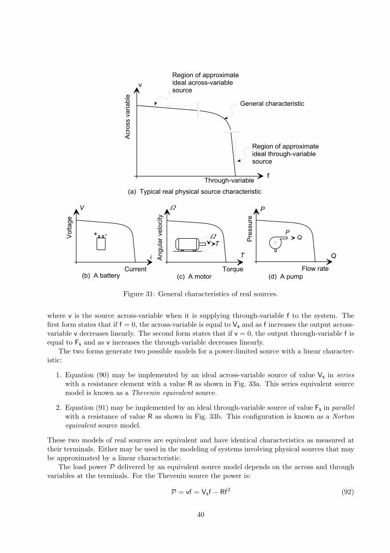
R e g i o n o f a p p r o x i m a t ei d e a l t h r o u g h - v a r i a b l es o u r c e

R e g i o n o f a p p r o x i m a t ei d e a l a c r o s s - v a r i a b l es o u r c ev

T h r o u g h - v a r i a b l e f

G e n e r a l c h a r a c t e r i s t i c

C u r r e n t T o r q u e F l o w r a t e

+ -T

W

T

W

V

i

QP

P

Q

( a ) T y p i c a l r e a l p h y s i c a l s o u r c e c h a r a c t e r i s t i c

( b ) A b a t t e r y ( c ) A m o t o r ( d ) A p u m p

Angu

lar ve

locity

Pres

sure

Acros

s vari

able

Volta

ge

Figure 31: General characteristics of real sources.

where v is the source across-variable when it is supplying through-variable f to the system. Thefirst form states that if f = 0, the across-variable is equal to Vs and as f increases the output across-variable v decreases linearly. The second form states that if v = 0, the output through-variable f isequal to Fs and as v increases the through-variable decreases linearly.

The two forms generate two possible models for a power-limited source with a linear character-istic:

1. Equation (90) may be implemented by an ideal across-variable source of value Vs in serieswith a resistance element with a value R as shown in Fig. 33a. This series equivalent sourcemodel is known as a Thevenin equivalent source.

2. Equation (91) may be implemented by an ideal through-variable source of value Fs in parallelwith a resistance of value R as shown in Fig. 33b. This configuration is known as a Nortonequivalent source model.

These two models of real sources are equivalent and have identical characteristics as measured attheir terminals. Either may be used in the modeling of systems involving physical sources that maybe approximated by a linear characteristic.

The load power P delivered by an equivalent source model depends on the across and throughvariables at the terminals. For the Thevenin source the power is:

P = vf = Vsf − Rf2 (92)

40

R

1

Outp

ut acr

oss

-variable

Output through-variable

f

v

V

o

F o

v = V - R f o s o s

s

Figure 32: Characteristic of a simple linear source.

System

R F (t) s

Through-variable source

System

R

V (t) s

Across-variable source

(a) Thevenin equivalent source (b) Norton equivalent source

Figure 33: Thevenin and Norton models of power-limited physical sources.

and for the Norton source it isP = vf = vFs − 1

Rv2 (93)

The maximum power an equivalent source can provide is found by differentiating Eq. (92) withrespect to f or Eq. (93) with respect to v and equating the derivative to zero. In either case themaximum power is supplied when f = Vs/2R and v = RFs/2. The maximum power supplied isPmax = VsFs/4.

Example

It has been found that the performance of the rotational flywheel drive model derivedin Example 10.2, with the linear graph shown in Fig. 25, does not adequately reflectthe dynamic response of the physical system over the full operating range of interest.Measurements on the system show that it is not valid to represent the motor as an idealangular velocity source over the full speed range. With a fixed supply voltage and noload, the motor spins at an angular velocity of Ωmax, but as the torque load is increasedthe motor speed decreases linearly until the shaft is stationary and generates a torqueTmax. Extend the linear graph model of Example 10.2 to include (a) a Thevenin and(b) a Norton source equivalent for the motor.

Solution: The measurements on the motor indicate that the source characteristic isas shown in Fig. 34.

41

J BB

W ( t )o

2 1W J

R1

WW

o

o

m a x

m a xT o r q u e T T

( a ) T h e m o t o r d r i v e s y s t e m ( b ) T h e m o t o r s o u r c e c h a r a c t e r i s t i c

Angu

lar ve

locity

Figure 34: The source characteristic of the electric motor.

The equivalent source resistance is found from the slope of the characteristic, that isR = Ωmax/Tmax. Figure 35 shows the two modified system linear graphs using (a) aThevenin and (b) a Norton source equivalent model for the motor. Both are equivalentwith respect to the dynamic behavior of the flywheel.

J

B

B 2

1

J

B

B 2

1

R

W max

T max R

(a) Thevenin source based model (b) Norton source based model

Figure 35: The rotational system of Fig. 4.11 redrawn with (a) a Thevenin equivalent source, and(b) a Norton equivalent source.

Thevenin and Norton source models may also be used to approximate the behavior of nonlinearphysical sources when the range of variation of the source variables is small. Consider a sourcewith a nonlinear characteristic

v = F(f) (94)

and assume that the source normally operates with small excursions about a nominal operatingpoint v = vo and f = fo. If Eq. (94) can be expanded as a Taylor series and the first two terms areretained

v ≈ vo +dF(f)

df

∣∣∣∣f=fo

(f − fo). (95)

If we define a D-type element

R∗ = − dF(f)df

∣∣∣∣f=fo

(96)

42

we can write an approximate source characteristic

v = vo − R∗(f − fo)= Vs − R∗f (97)

where Vs = vo + R∗fo. Equation (97) defines a Thevenin equivalent source with an ideal source Vs

and a series resistance R∗. A linearized Norton source can also be expressed as a through-variablesource Fs = fo + (1/R∗)vo in parallel with a D-type element R∗.

References:

1. Firestone, F.A., “A New Analogy Between Mechanical and Electrical Systems,” Journal ofthe Acoustic Society Am., pp. 248-264, 1963.

2. Trent, H.M., “Isomorphisms Between Oriented Linear Graphs and Lumped Physical Sys-tems,” Journal of the Acoustic Society Am., pp. 500-527, 1955.

3. Shearer, J.L., Murphy, A.T., Richardson, H.H., Introduction to System Dynamics, Addison-Wesley Publishing Company, Reading, MA, 1967.

4. Koenig, H.E., Tokad, Y., Kesavan, H.K, Hedges, H.C., Analysis of Discrete Physical Systems,McGraw-Hill Book Company, New York, NY, 1967.

5. Blackwell, W.A., Mathematical Modeling of Physical Networks, Macmillan Publishing Com-pany, New York, NY, 1968.

6. Paynter, H.M., Analysis and Design of Engineering Systems, MIT Press, Cambridge, MA,1961.

7. Karnopp, D.C., Margolis, D.L, Rosenberg, R.C., System Dynamics: A Unified Approach(Second Edition), John Wiley & Sons Inc., New York, NY, 1990.

43