Lifetime analysis of wireless sensor nodes in different smart grid environments

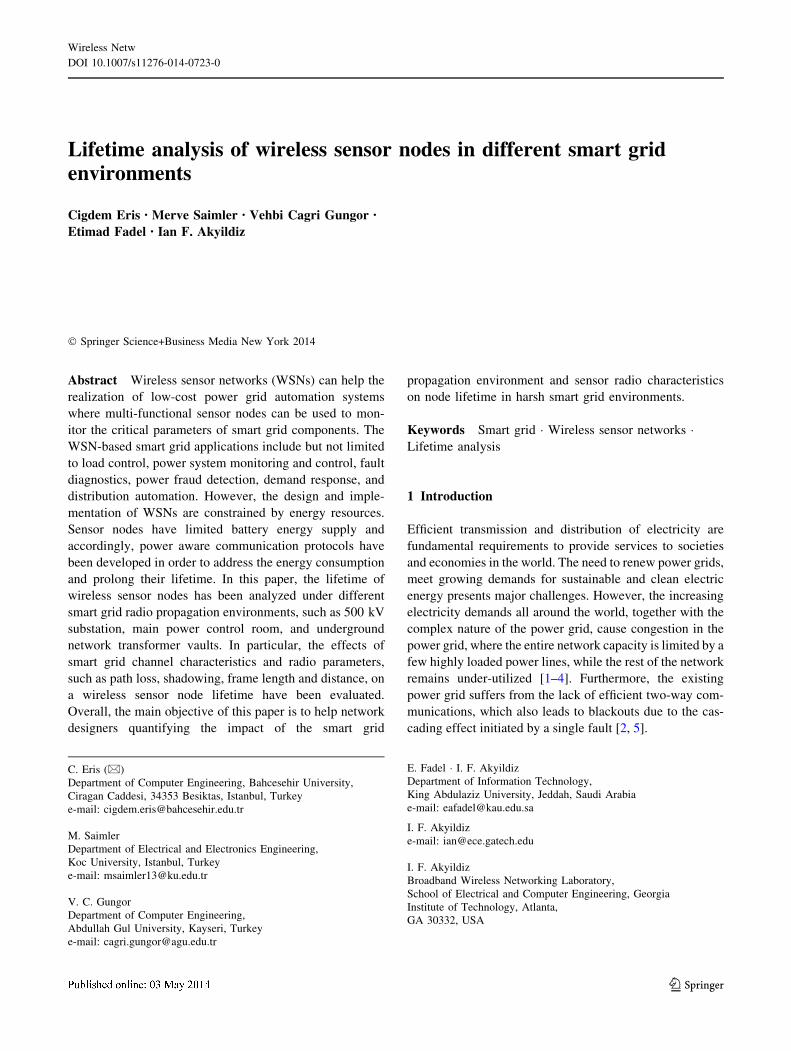
Lifetime analysis of wireless sensor nodes in different smart gridenvironments

Cigdem Eris • Merve Saimler • Vehbi Cagri Gungor •

Etimad Fadel • Ian F. Akyildiz

� Springer Science+Business Media New York 2014

Abstract Wireless sensor networks (WSNs) can help the

realization of low-cost power grid automation systems

where multi-functional sensor nodes can be used to mon-

itor the critical parameters of smart grid components. The

WSN-based smart grid applications include but not limited

to load control, power system monitoring and control, fault

diagnostics, power fraud detection, demand response, and

distribution automation. However, the design and imple-

mentation of WSNs are constrained by energy resources.

Sensor nodes have limited battery energy supply and

accordingly, power aware communication protocols have

been developed in order to address the energy consumption

and prolong their lifetime. In this paper, the lifetime of

wireless sensor nodes has been analyzed under different

smart grid radio propagation environments, such as 500 kV

substation, main power control room, and underground

network transformer vaults. In particular, the effects of

smart grid channel characteristics and radio parameters,

such as path loss, shadowing, frame length and distance, on

a wireless sensor node lifetime have been evaluated.

Overall, the main objective of this paper is to help network

designers quantifying the impact of the smart grid

propagation environment and sensor radio characteristics

on node lifetime in harsh smart grid environments.

Keywords Smart grid � Wireless sensor networks �Lifetime analysis

1 Introduction

Efficient transmission and distribution of electricity are

fundamental requirements to provide services to societies

and economies in the world. The need to renew power grids,

meet growing demands for sustainable and clean electric

energy presents major challenges. However, the increasing

electricity demands all around the world, together with the

complex nature of the power grid, cause congestion in the

power grid, where the entire network capacity is limited by a

few highly loaded power lines, while the rest of the network

remains under-utilized [1–4]. Furthermore, the existing

power grid suffers from the lack of efficient two-way com-

munications, which also leads to blackouts due to the cas-

cading effect initiated by a single fault [2, 5].

C. Eris (&)

Department of Computer Engineering, Bahcesehir University,

Ciragan Caddesi, 34353 Besiktas, Istanbul, Turkey

e-mail: [email protected]

M. Saimler

Department of Electrical and Electronics Engineering,

Koc University, Istanbul, Turkey


V. C. Gungor

Department of Computer Engineering,

Abdullah Gul University, Kayseri, Turkey


E. Fadel � I. F. Akyildiz

Department of Information Technology,

King Abdulaziz University, Jeddah, Saudi Arabia


I. F. Akyildiz


I. F. Akyildiz

Broadband Wireless Networking Laboratory,

School of Electrical and Computer Engineering, Georgia

Institute of Technology, Atlanta,

GA 30332, USA

123

Wireless Netw

DOI 10.1007/s11276-014-0723-0

To address all these challenges, a new concept of next

generation electric power system, a smart grid, has been

proposed [2]. The smart grid is a modern power grid

infrastructure for enhanced reliability, productivity, and

safety through automated controls and modern communi-

cation technologies. Considering the large scale of the

electric power grid, low-cost monitoring and control

enabled by real-time sensing technologies have become

essential to maintain the efficiency of the smart grid.

With the recent advances in wireless sensor networks

(WSNs), the realization of low-cost embedded power grid

automation systems have become feasible. In these sys-

tems, wireless multi-functional sensor nodes have been

used to monitor the critical parameters of smart grid

components [6–9]. The WSN-based smart grid applications

include power system monitoring and control, power fraud

detection, demand response, load control, fault diagnostics

and distribution automation [2, 10–13]. However, the

design and implementation of WSNs are constrained by

energy resources [14, 15]. In general, sensor nodes have

limited battery energy supply and thus, communication

protocols for WSNs are mainly tailored to provide high

energy efficiency.

In this paper, the lifetime of wireless sensor nodes has

been analyzed under different smart grid radio propagation

environments, such as 500 kV substation, main power

control room, and underground network transformer vaults.

Although there exists sensor node lifetime analysis for

different sensor hardware architectures, none of them

addresses how different smart grid radio propagation

environments affect the network lifetime of the corre-

sponding smart grid application. Analyzing the lifetime of

sensor nodes in terms of different radio and network

parameters and smart grid spectrum characteristics gives a

new impulse to ongoing research topics. Overall, the main

objective of this paper is to help network designers quan-

tifying the impact of the smart grid propagation environ-

ment and sensor radio characteristics on node lifetime in

harsh smart grid environments. The main contributions of

our study can be itemized as follows:

• The effects of smart grid channel characteristics and

radio parameters, such as path loss, shadowing devia-

tion, frame length and distance, on a wireless sensor

node lifetime have been evaluated.

• The challenges on deploying schedule-driven wireless

sensor networks in smart power grid environments have

been explained to estimate the node lifetime.

• In addition to smart grid environment characteristics,

the impact of different operation modes of sensor nodes

on network lifetime has been discussed.

The remainder of this paper is organized as follows. In

Sect. 2, we present an overview of the related work on

wireless sensor node lifetime. In Sect. 3 we introduce the

new method and protocol. In Sect. 4, we present the

mathematical model and evaluate the performance of our

solutions. Finally, we conclude the paper in Sect. 5.

2 Related work on lifetime estimation in wireless sensor

networks

One of the major research activities within the area of

wireless sensor networks was based on lifetime analysis in

the last decade. In [16], a two sensor node network is

modeled and trigger-driven and schedule-driven nodes, are

analyzed for power consumption and the solutions are

validated by using the simulation tool, MATSNL. Based on

the work of [16], the lifetime is also taken into consider-

ation within the context of availability and security in [17].

Alhtough the existing lifetime models are applicable in

networks to meet certain specified conditions, they do not

deal with how environmental spectrum characteristics

affect the network lifetime and average power consumption

per node. Wireless channel propagation characteristics are

as much important as hardware specifications as stated in

[18]. In order to conduct an accurate analysis, the power

dissipation of a node should be analyzed by considering the

wireless channel parameters.

Specifically, different deployment environments and

indicative parameters are essential to analyze power con-

sumption of a node. The main indicative parameters that

affect sensor networks include network coverage, event

detection ratio, quality of services parameters (QoS), con-

nectivity (availability, latency, loss), requirements for

continuous service (service disruptions up to a length) and

the observation accuracy (measurement errors). Additional

parameters, such as link asymmetry and channel charac-

teristics, have been considered in our work to calculate

more accurate power consumption of sensor nodes.

In recent years, existing platforms improved new tech-

niques for reducing power leakage on sleep mode and dual

pre-processor/radio architecture to analyze power efficient

and high-power components as XYZ in [19], LEAP in [20],

iMote2 in [21]. Moreover, an energy management and

accounting preprocessor (EMAP) module enables to con-

struct different power modes on sensors. In addition, the

detailed simulation tool PowerTOSSIM computes the

power consumption with a low error margin. In [22, 12],

the schedule-based energy consumption is shown for target

tracking application [23].

In [24], a demonstrator of a wireless sensor network for

smart grid applications is introduced. It explains the

hardware of the sensor nodes and demonstrates the results

of the performance activity with the assurance of the fea-

sibility of the recommended solutions. In [25] a system

Wireless Netw

123

analysis is provided with a solution to the problem of

controlling the sleep-awake period of nodes optimally. The

proposed solution aims to extend the node life time as well

as the network lifetime based on the constraint of the end-

to-end packet delivery delay.





sponding smart grid application. Analyzing the lifetime of

sensor nodes in terms of different radio and network

parameters and smart grid spectrum characteristics gives a

new impulse to ongoing research topics.

3 Evaluated methods and protocols

In the literature, different lifetime models, such as event-

driven and schedule driven models, are used to evaluate the

lifetimes of WSNs. In particular, a set of sensor hardware

parameters, such as power consumption per task, state

transition overhead and communication cost, are used to

compute the average lifetime of a node for a given event

arrival rate. In general, five different power states are

commonly used for each lifetime model. In event-driven

model, the pre-processor is always on and the node is in a

deep sleep mode. The node is in the awake state if and only

if an event is detected. In the schedule driven node, the

duty cycle is described as awake time/duty period. The

node is sleeping most of the time of operation and sleeps

until the node wake-up timer expires. In our model, the

power state transitions are described as a Semi-Markov

chain and the following assumptions are made:

• The first-order statistical characteristic (mean value) of

all random quantities (events, processing time, etc.) is

known by observation and experiment.

• The processing and communication time is short

compared to inter-arrival time of events. Processing

and radio-transmission times are independent and

identically distributed.

• The event duration is zero for an impulse event. We assume

all events in the schedule-driven mode as an impulse event.

• The zero event durations make the duty cycle equal to

the detection probability. The modulation scheme is

orthogonal quadrature phase shift keying (O-QPSK). It

is used in Telos with direct sequence spread spectrum

(DSSS), which provides much more sophisticated

mechanism for sensor networks [26, 12].

• CSMA MAC protocol is used to calculate the average

power consumption of an individual packet transmis-

sion. During each communication period, the sensor

resides in a limited number of low power states.

To model wireless channel in smart grid environments, we

also used the wireless channel model and parameters

determined in our previous study via field-test experiments

[2]. In this model, signal to noise ratio cðdÞ at a distance

d from the transmitter is given by the equation [27]:

cðdÞdB ¼ Pt � PLðd0Þ � 10g log10

d

d0

� Xr � Pg ð1Þ

where Pt is the transmit power, PLðd0Þ is the path loss at a

reference distance d0, g is the path-loss exponent, Xr is a

zero mean Gaussian random variable with standard devi-

ation r and Pg is the noise power (noise floor), in which all

powers are in dBm.

In this section, we investigate the lifetime of wireless

sensor nodes in smart grid with respect to different power

system environments. For the performance evaluation, we

modified the Matlab simulation environment MATSNL

[16, 28] to evaluate the effects of the propagation charac-

teristics on node lifetime in different smart grid environ-

ments. The node is determined to work as a schedule-

driven node in which its period of working is determined

by a timer which indicates the time period as if the node is

in the active mode Timerawake or in sleep mode Timersleep.

Schedule-driven node working mechanism consists of six

different modes as seen in Table 1. The smart grid channel

parameters we used in our performance analysis are listed

in Table 2 and the power consumption of each mode is

presented in Table 3.

Importantly, according to the mode definitions, there

should be more definitions stated in order to get an under-

standing of the whole picture of schedule-driven nodes.

There are transitions between different states with certain

probabilities. Demonstration of the power transition of a

schedule-driven node, which is formed as Semi-Markov

chain as shown in Fig. 1 helps to examine the power state

transitions [16]. Beginning with the assumption that the node

is awake, when if there is a b probability event present then it

would be stated that the event would be detected.

As the next step, the sensor transits to S4e, which is called

as the monitoring state. In this case, the preprocessor and the

sensor is working, CPU is idle and the radio component of the

node is not in process After monitoring state, the mechanism

would certainly transit to the processing state, S2, which

Table 1 Modes of a schedule-

driven nodeModes Sensor CPU Radio

S0 Off Off Off

S1 – – –

S2 On On Off

S3 On On Tx

S4 On Idle Off

S5 On On Rx

Wireless Netw

123

forces the CPU to turn on. Following this state, the operating

mode of the sensor is S3 if the sensed event has data to be sent

to the base station (BS) which has the a probability and the

radio component turns on. On the other hand, if the proba-

bility 1-a happens to occur that the sensed event has no data

to be transferred to BS, then the sensor node transits to the

sleep state. Lastly, the data sent to BS is processed at the

communication state and transition to sleep state with

probability 1 which completes cycle of the Semi-Markov

chain. In addition to the assumption that the node is awake 1-

b is the probability when there is not any sensed event in the

medium. In this case, the node transits to S4i and in return, it

transits back to the sleep state as Timersleep takes over its

duty.

Importantly, to get a better understanding of the mech-

anism of the schedule-driven mode node, the average

consumed power should be examined. Since the consumed

power is highly related to the detection probability of the

events sensed in the medium, the mechanism is stated with

comparison to trigger-driven mode node in terms of

detection probability and average consumed power in [16].

As shown in Table 4, Tc indicates the duration of the duty

cycle d, Tw shows the awake period of the node, whereas Ts

shows the sleep period of the node and u is the detection

probability of an event. Lastly, as mentioned before, kindicates the poisson arrival rate of the events to the

specified medium. The consumed power does not vary with

the varying detection probability for the case trigger-driven

mode nodes but on the contrary the power consumption of

schedule-driven nodes changes because its transition

mechanism is led by the timer. Overall, all the important

parameters affecting sensor node lifetime are summarized

in Table 4. In order to examine the average consumed

power in a more detailed way, the related definitions are

stated as follows:

• Me is the residual energy that can be specified as the

rest of the energy consumed in a cycle in which the

node is awake. It can be formulated as:

Me ¼ Pw � Tw � ðTw � ðPs2þ Ps3

ÞÞ ð2Þ

where Pw is the consumed power when the node is in

the awake period, Ps2is the power consumed in the

processing state and Ps3is the power consumed in the

communication State.

• Mt is the residual time. In a cycle, the operation of a

node takes a determined time and the rest time of the

node is called as Mt, which is formulated as:

Mt ¼ Tw � ðTs2þ Ts3

Þ=ðTs2Þ ð3Þ

where Ts2is the time spent in the processing state and

Ts3is the time spent in the communication state.

Note that the major parameter that changes the node

lifetime is the transmission power of the node, since the

Table 2 Path loss exponent and shadowing deviation in smart grid

environments

Propagation environment Path

loss (g)

Shadowing

deviation (r)

Noise

floor (Pn)

500 kV substation (LOS) 2.42 3.12 -93

500 kV substation

(NLOS)

3.51 2.95 -93

Underground transformer

vault (LOS)

1.45 2.45 -92

Underground transformer

vault (NLOS)

3.15 3.19 -92

Main power room (LOS) 1.64 3.29 -88

Main power room (NLOS) 2.38 2.25 -88

Table 3 Schedule driven sensor node power specifications

Sensor Mica2 Telos Imote2 XYZ

Microcontroller ATMega128 TIMSP430 PXA271 ML67 ARM/THUMB

CPU ON (mW) 24 2.7 193 41

CPU IDLE (mW) 9.6 0.09 88 34

CPU OFF (mW) 0.3 0.0018 1.8 0.0063

CPU wake up time (ls ) 180 6 860.11 252

Radio CC1000 CC2420 CC2420 CC2420

Tx 25.5 35 70 57

Rx 21 38 80 65

Idle 0.7 0.7 0.7 0.7

Wake up time(ls) 180,000 580 860 860

Data rate 38.4 250 250 250

Modulation FSK O-QPSK O-QPSK O-QPSK

Processing time 0.2 0.2 0.2 0.6

Wireless Netw

123

power consumption during communication mode is very

high compared to other operation modes. Moreover, when

the channel conditions are bad and packet losses occur, the

node retransmits the data packet to reliably transmit the

message. All these retransmissions cause further power

consumption for the sensor node. Therefore, to estimate the

lifetime of a node accurately, the impact of radio propa-

gation and environmental characteristics on packet recep-

tion rate should be considered. Here, the packet reception

rate (PRR) represents the ratio of the number of successful

packets to the total number of packets transmitted over a

certain number of transmissions. Note that combining bit

error rates together with the corresponding encoding

schemes ; the packet reception rate (PRR) for different

sensor motes can be calculated. It is also important to note

that different from earlier platforms, the modulation

scheme of the recent sensor node platforms is based on

IEEE 802.15.4 standard, which uses orthogonal quadrature

phase shift keying (O-QPSK) with direct sequence spread

spectrum (DSSS), providing much more sophisticated

mechanism for the sensor networks. For example, the

modulation scheme used in Telos nodes is offset O-QPSK

with DSSS. O-QPSK with DSSS modulation scheme in

[29], where K is the number of users who are transmitting

simultaneously and N is the number of chips per bit.

POQPSKb ¼ Qð

ffiffiffiffiffiffiffiffiffiffiffiffiffiffiffiffiffiffiffiffiffiffiffiffiffiffi

ððEb=NoÞDSÞq

Þ ð4Þ

where

ðEb=NoÞDS ¼ð2N � Eb=NoÞ

ðN þ 4Eb=NoðK � 1Þ=3Þ ð5Þ

Combining the bit error rates together with the corre-

sponding encoding scheme NRZ; the packet reception rate

(PRR) for different sensor nodes can be calculated as

shown in [27]:

PRR ¼ ð1� PbÞ8lð1� PbÞ8ðf�lÞ ð6Þ

In the following section, considering all above-men-

tioned assumptions , we analyze the lifetime of wireless

sensor nodes in smart grid environments based on smart

grid channel characteristics (such as path loss, shadowing

deviation, etc.), sensor operation states and modes, as well

as network parameters (duty cycle, event arrival rate,

packet reception rate, frame length and distance, etc.).





sponding smart grid application. When considering the

propagation characteristics, we believe that the researchers

can achieve more accurate lifetime estimations. Thus,

analyzing the lifetime of sensor nodes in terms of different

radio and network parameters and smart grid spectrum

characteristics will give a new impulse to ongoing research

topics.

Fig. 1 Semi-Markov chain

power state transition model of

a schedule driven node

Table 4 List of simulation parameters

Parameter Definition

b Probability of an event present in the cell

d Duty cycle

Me Residual energy

Mt Residual time

Pw Consumed power when the node is awake

Pe Average power consumption when there is no events are

detected

Ps2Consumed power in the processing state

Ps3Consumed power in the communication state

Tc Duration of duty cycle

Ts Sleep period of node

Tw Awake period of node

Ts2Time spent in the processing state

Ts3Time spent in the communication state

Ntx Number of retransmissions

TL Expected life time

u Detection probability

Wireless Netw

123

4 Performance evaluations

Our performance evaluation is based on experimentally

determined lognormal channel parameters from our previ-

ous work [2], where the wireless channel in different smart

grid environments was modeled through real-world field

tests by using the IEEE 802.15.4 compliant wireless sensor

nodes in different electric power system environments such

as such as 500 kV substation, main power control room,

and underground network transformer vaults.

We compared lifetime of a schedule-driven Telos under

six different smart grid environments. In Fig. 2(a), (b), we

00.2

0.40.6

0.81

00.2

0.40.6

0.81

10−1

100

101

102

103

Duty CyclePacket reception rate

Life

time

(day

)TelosMica2Imote2XYZ

00.2

0.40.6

0.81

10−210

−110010

1102

10−2

100

102

104

Duty CycleArrival Rate(1/hour)

Life

time(

day)

TelosMica2Imote2XYZ(a) (b)

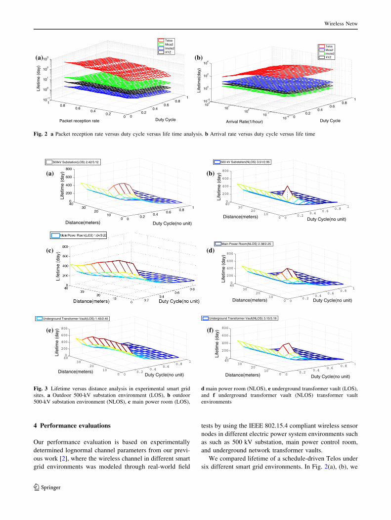
Fig. 2 a Packet reception rate versus duty cycle versus life time analysis. b Arrival rate versus duty cycle versus life time

00.2

0.40.6

0.81

010

2030

400

200

400

600

800

Duty Cycle(no unit) Distance(meters)

Life

time

(day

)

500kV Substation(LOS) 2.42/3.12

00.2

0.40.6

0.81

010

2030

400

200

400

600

800

Duty Cycle(no unit) Distance(meters)Li

fetim

e (d

ay)

500 kV Substation(NLOS) 3.51/2.95

(a) (b)

00.2

0.40.6

0.81

010

2030

400

200

400

600

800


Life

time

(day

)

Main Power Room(NLOS) 2.38/2.25

(d)

00.2

0.40.6

0.81

010

2030

400

200

400

600

800


Life

time

(day

)

Underground Transformer Vault(LOS) 1.45/2.45

00.2

0.40.6

0.81

010

2030

400

200

400

600

800


Life

time

(day

)

Underground Transformer Vault(NLOS) 3.15/3.19

(e) (f)

(c)

Fig. 3 Lifetime versus distance analysis in experimental smart grid

sites. a Outdoor 500-kV substation environment (LOS), b outdoor

500-kV substation environment (NLOS), c main power room (LOS),

d main power room (NLOS), e underground transformer vault (LOS),

and f underground transformer vault (NLOS) transformer vault

environments

Wireless Netw

123

observe that the increasing distance at a fixed value of a

duty period, decreases the lifetime. In these figures, we see

that increasing the arrival rate and duty cycle decreases the

lifetime of different nodes, since the event detection

probability increases during the awake period at each node.

We also observed that the maximum lifetime is obtained

from Telos node due to its low energy consumption in both

processing and idle stages compared to other sensor nodes.

Note that Mica2, XYZ and Imote2 consume much more

power in processing and idle stages. The lifetime duration

of Mica2 suffers from the wake up time, which is too high

compared to other nodes.

In the following, we continue our lifetime evaluations

with Telos nodes, since it has longer lifetime compared to

other nodes. As shown in Fig. 3(a)–(f), increasing duty

cycle decreases lifetime exponentially, since the node is

continuously sampling during the awake period. Increasing

duty period in WSNs exponentially decreases the network

lifetime. Additionally, we show the network lifetime with

varying communication distance and duty cycle for dif-

ferent smart grid environments. In these figures, we see that

the maximum lifetime of a node is around 835 days. In

addition, increasing inter arrival rate with a duty cycle

(increasing the awake time during duty period) decreases

the lifetime of the node, since the detection probability of

the awake node becomes higher. The high detection

probabilities consume more power as compared to lower

duty cycles.

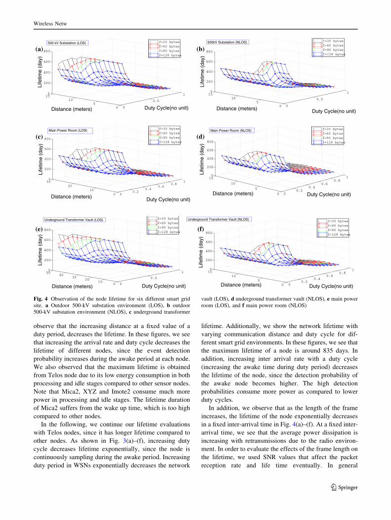
In addition, we observe that as the length of the frame

increases, the lifetime of the node exponentially decreases

in a fixed inter-arrival time in Fig. 4(a)–(f). At a fixed inter-

arrival time, we see that the average power dissipation is

increasing with retransmissions due to the radio environ-

ment. In order to evaluate the effects of the frame length on

the lifetime, we used SNR values that affect the packet

reception rate and life time eventually. In general

0

0.5

1

05

10150

200

400

600

800

Duty Cycle(no unit)Distance (meters)

Life

time

(day

)f=30 bytesf=60 bytesf=90 bytesf=128 bytes

500 kV Substation (LOS)

0

0.5

1

05

10150

200

400

600

800


Life

time

(day

)

f=30 bytesf=60 bytesf=90 bytesf=128 bytes

500kV Substation (NLOS)

(a) (b)

00.2

0.40.6

0.81

010

20300

200

400

600

800


Life

time

(day

)


Main Power Room (LOS)

00.2

0.40.6

0.81

0

5

10

150

200

400

600

800

Duty Cycle(no unit)Distance (meters)Li

fetim

e (d

ay)


Main Power Room (NLOS)

(c) (d)

0

0.5

1

010

2030

40500

200

400

600

800


Life

time

(day

)


Underground Transformer Vault (LOS)

00.2

0.40.6

0.81

05

10150

200

400

600

800


Life

time

(day

)


Underground Transformer Vault (NLOS)

(e) (f)

Fig. 4 Observation of the node lifetime for six different smart grid

site. a Outdoor 500-kV substation environment (LOS), b outdoor

500-kV substation environment (NLOS), c underground transformer

vault (LOS), d underground transformer vault (NLOS), e main power

room (LOS), and f main power room (NLOS)

Wireless Netw

123

increasing the SNR value, small size of frame length

increases packet reception rate compared to large size of

frame lengths.

In summary, our performance evaluation demonstrates

that the smart grid channel parameters, such as path loss

exponent and shadowing, directly affect the lifetime of a

schedule-driven node in smart grid environments. We

compared the lifetime of a schedule-driven Telos in six

different smart grid environments. The overall lifetime of the

network is vulnerable for the propagation characteristics of

the smart grid environment. As shown in the above men-

tioned figures, increasing the duty cycle decreases the life-

time exponentially, since the node is continuously sampling

during the awake period in terms of detection probability of

an event. Without considering the channel conditions, the

lifetime is only related to duty cycle, duty period and arrival

time of events. While considering the propagation charac-

teristics, we believe that the researchers can achieve more

accurate lifetime estimations. We calculate the lifetime by

considering the packet reception rates, which affect the total

number of transmitted packets per sensed event. Increasing

the distance among nodes decreases the received power of

the signal, which decreases exponentially with increasing

path loss exponent. We also observe that the lifetime chan-

ges due to channel conditions in different environments.

Furthermore, the high path loss environments have a nega-

tive impact on the network lifetime.

5 Conclusions

With the recent advances in wireless sensor networks

(WSNs), the realization of low-cost embedded power grid

automation systems have become feasible. In these sys-

tems, wireless multi-functional sensor nodes have been

used to monitor the critical parameters of smart grid

components. The WSN-based smart grid applications

include power fraud detection, demand response, power

system monitoring and control, load control, fault diag-

nostics and distribution automation. However, the design

and implementation of WSNs are constrained by energy

resources. In general, sensor nodes have limited battery

energy supply and thus, communication protocols for

WSNs are mainly tailored to provide high energy effi-

ciency. In this paper, the lifetime of wireless sensor nodes

has been analyzed under different smart grid radio propa-

gation environments, such as 500 kV substation, main

power control room, and underground network transformer

vaults. Specifically, sensor node lifetime is analyzed in

terms of smart grid channel characteristics (such as path

loss, shadowing deviation, etc.), sensor operation states and

modes, as well as network parameters (duty cycle, event

arrival rate, packet reception rate, frame length and

distance, etc.). Although there exists sensor node lifetime

analysis for different sensor hardware architectures, none

of them addresses how different smart grid radio propa-

gation environments affect the network lifetime of the

corresponding smart grid application. Overall, the main

objective of this paper is to help network designers quan-

tifying the impact of the smart grid propagation environ-

ment and sensor radio characteristics on node lifetime in

harsh smart grid environments.

Acknowledgments This paper was funded by KACST through The

National Policy for Science, Technology and Innovation Plan, under

Grant No. (12-INF2731-03). The authors, therefore, acknowledge

technical and financial support of KACST and the Unit for Science

and Technology at KAU.

References

1. Calderaro, V., Hadjicostis, C., Piccolo, A., & Siano, P. (2011).

Failure identification in smart grids based on petri net modeling.

IEEE Transactions Industrial Electronics, 58(10), 4613–4623.

2. Gungor, V. C., Lu, B., & Hancke, G. P. (2010). Opportunities and

challenges of wireless sensor networks in smart grid. IEEE

Transactions on Industrial Electronics, 57(10), 3557–3564.

3. Gungor, V. C., Sahin, D., Kocak, T., Ergut, S., Buccella, C.,

Cecati, C., et al. (2012). A survey on smart grid potential appli-

cations and communication requirements. IEEE Transactions on

Industrial Informatics, 9(1), 28–42.

4. Gungor, V. C., Sahin, D., Kocak, T., Ergut, S., Buccella, C.,

Cecati, C., et al. (2011). Smart grid technologies: Communication

technologies and standards. IEEE Transactions on Industrial

Informatics, 7(4), 529–539.

5. Gungor, V. C., & Hancke, G. (2009). Industrial wireless sensor

networks: Challenges, design principles, and technical approa-

ches. IEEE Transactions on Industrial Electronics, 56(10),

4258–4265.

6. Akyildiz, I. F., Su, W., Sankarasubramaniam, Y., & Cayirci, E.

(2002). Wireless sensor networks: A survey. Computer Networks,

38(4), 393–422.

7. De Couto, D. S. J., Aguayo, D., Bicket, J., & Morris, R. (2003). A

high-throughput path metric for multi-hop wireless routing. In

ACM MobiCom 03, San Diego, CA.

8. Kim, J., Lin, X., Shroff, N. B., & Sinha, P. (2010). Minimizing

delay and maximizing lifetime for wireless sensor networks with

anycast. IEEE/ACM Transactions on Networking, 18(2),

515–528.

9. Tuna, G., Gungor, V. C., & Gulez, K. (2013). Wireless sensor

networks for smart grid applications: A case study on link reli-

ability and node lifetime evaluations in power distribution sys-

tems. Hindawi Publishing Corporation International Journal of

Distributed Sensor Networks (Article ID 796248).

10. Guo, F., Herrera, L., Murawski, R., Inoa, E., Wang, C., Beau-

champ, P., et al. (2013). Comprehensive real time simulations of

smart grid. IEEE Transactions on Industry Applications, 49(2),

899–908.

11. Shah, G. A., Gungor, V. C., & Akan, O. B. (2013). A cross-layer

QoS-aware communication framework in cognitive radio sensor

networks for smart grid applications. IEEE Transactions on

Industrial Informatics, 9(3), 1477–1485.

12. Wu, K., Tan, H., Ngan, Hoi-Lun, Liu, Y., & Ni, L. M. (2012).

Chip error pattern analysis in IEEE 802.15.4. IEEE Transactions

on Mobile Computing, 11(4), 543–552.

Wireless Netw

123

13. Wang, W., Xu, Y., & Khanna, M. (2011). A survey on the

communication architectures in smart grid. Computer Networks

Journal, 55, 3604–3629.

14. Vaccaro, A., Velotto, G., & Zobaa, A. (2011). A decentralized

and cooperative architecture for optimal voltage regulation in

smart grids. IEEE Transactions Industrial Electronics., 58(10),

4593–4602.

15. Gungor, V. C., & Lambert, F. C. (2006). A survey on commu-

nication networks for electric system automation. Computer

Networks, 50(7), 877–897.

16. Teixeira, T., Jung, D., & Savvides, A. (2009). Sensor node life-

time analysis: Models and tools. ACM Transactions on Sensor

Networks, 5(1), 1–29.

17. Khan, M., & Misic, J. (2007). Security in IEEE 802.15.4 cluster

based networks. In Y. Zhang, J. Zheng, & H. Hu (Eds.), Security

in wireless mesh networks. Wireless Networks and Mobile

Communications (Vol. 6). Boca Raton, FL: Auerbach Publica-

tions, CRC Press.

18. Dietrich, I., & Dressler, F. (2009). On the life-time of wireless

sensor networks. ACM Transactions on Sensor Networks (TOSN),

5(1):39. doi:10.1145/1464420.1464425 (Arcticle 5).

19. Lymberopoulos, D., & Savvides, A. (2005). Xyz: A motion-

enabled, power aware sensor node plat- form for distributed

sensor network applications. In 4th International symposium on

information processing in sensor networks (IPSN), Vol. 15 (pp.

449–454).

20. McIntire, D., Ho, K., Yip, B., Singh, A., Wu, W., & Kaiser, W. J.

(2005). The low power energy aware processing (LEAP)

embedded networked sensor system. In Proceedings of the

information processing in sensor networks (IPSN/SPOTS).

21. Nachman, L., Huang, J., Shahabdeen, J., & Adler R. (2008).

IMOTE2: Serious computation at the edge. In IWCMC ’08

International wireless communications and mobile computing

conference 2008 (pp. 1118–1123).

22. Vicaire, P., He, T., Cao, Q., Yan, T., Zhou, G., Gu, L., et al.

(2009). Achieving long-term surveillance in VigilNet. ACM

Transactions on Sensor Networks, Vol. 5, No. 1, (Article 9).

23. Zaballos, A., Vallejo, A., & Selga, J. M. (2011). Heterogeneous

communication architecture for the smart grid. IEEE Network,

25(5), 30–37.

24. Grilo, A., Sarmento, H., Nunes, M., Gonalves, J., Pereira, P.,

Casaca, A., et al. (2012). A wireless sensors suite for smart grid

applications. In International workshop on information technol-

ogy for energy, pp. 11–20.

25. Fadlullah, Z. M., Fouda, M. M., Kato, N., Takeuchi, A., Iwasaki,

N., & Nozaki, Y. (2011). Toward intelligent machine-to-machine

communications in smart grid. IEEE Communications Magazine,

49(4), 60–65.

26. Gungor, V. C., & Sahin, D. (2012). Cognitive radio networks for

smart grid applications: A promising technology to overcome

spectrum inefficiency. IEEE Vehicular Technology Magazine,

7(2), 41–46.

27. Rappapport, T. (2002). Wireless communications: Principles and

practice. New Jersey: Prentice Hall.

28. Zuniga, M., & Krishnamachari, B. (2007). An analysis of unre-

liability and asymmetry in low-power wireless links. ACM

Transactions on Sensor Networks (TOSN), 3(2).

29. Vuran, M. C., & Akyildiz, I. F. (2009). Error control in wireless

sensor networks: A cross layer analysis. IEEE/ACM Transactions

on Networking, 17(4), 1186–1199.

Cigdem Eris is a Ph.D. student

in Computer Engineering at

Bahcesehir University, Istanbul,

Turkey. Her current research

interests are smart grid commu-

nications, wireless adhoc and

sensor networks.

Merve Saimler is a Ph.D. stu-

dent in Electrical and Electronics

Engineering at Koc University,

Istanbul, Turkey. Her current

research interests are wireless

networks, smart grid communi-

cations, wireless adhoc and sen-

sor networks.

Vehbi Cagri Gungor received

his B.S. and M.S. degrees in

Electrical and Electronics Engi-

neering from Middle East Tech-

nical University, Ankara, Turkey,

in 2001 and 2003, respectively.

He received his Ph.D. degree in

electrical and computer engi-

neering from the Broadband and

Wireless Networking Laboratory,

Georgia Institute of Technology,

Atlanta, GA, USA, in 2007. Cur-

rently, he is an Associate Profes-

sor and Chair of Computer

Engineering Department, Abdul-

lah Gul University (AGU), Kayseri, Turkey. His current research inter-

ests are in smart grid communications, machine-to-machine

communications, next-generation wireless networks, wireless ad hoc and

sensor networks, cognitive radio networks, and IP networks. Dr. Gungor

has authored several papers in refereed journals and international con-

ference proceedings, and has been serving as an editor, reviewer and

program committee member to numerous journals and conferences in

these areas. He is also the recipient of the IEEE Trans. on Industrial

Informatics Best Paper Award in 2012, IEEE ISCN Best Paper Award in

2006, the European Union FP7 Marie Curie RG Award in 2009, Turk

Telekom Research Grant Awards in 2010 and 2012, and the San-Tez

Project Awards supported by Alcatel-Lucent, and the Turkish Ministry of

Science, Industry and Technology in 2010.

Wireless Netw

123

http://dx.doi.org/10.1145/1464420.1464425

Etimad Fadel received the Bachelors degree in Computer Science at

King Abdul Aziz University with Senior Project title ATARES:

Arabic Character Analysis and Recognition in 1994. She was awarded

the M.phil./ Ph.D. degree in computer science at De Montfort

University (DMU) with Thesis title Distributed Systems Management

Service in 2007. Currently, she is working as Assistant Professor at

the Computer Science Department at KAU. Her main research

interest is distributed systems, which are developed based on

middleware technology. Currently she is looking into and working

on Wireless Networks, Internet of Things and Internet of Nano-

Things.

Ian F. Akyildiz received the

B.S., M.S., and Ph.D. degrees in

Computer Engineering from the

University of Erlangen-Nrn-

berg, Germany, in 1978, 1981

and 1984, respectively. Cur-

rently, he is the Ken Byers

Chair Professor in Telecommu-

nications with the School of

Electrical and Computer Engi-

neering, Georgia Institute of

Technology, Atlanta, the Direc-

tor of the Broadband Wireless

Networking Laboratory and

Chair of the Telecommunication

Group at Georgia Tech. Dr. Akyildiz is an honorary professor with the

School of Electrical Engineering at Universitat Politcnica de Ca-

talunya (UPC) in Barcelona, Catalunya, Spain and the founder of

N3Cat (NaNoNetworking Center in Catalunya). He is also an hon-

orary professor with the Department of Electrical, Electronic and

Computer Engineering at the University of Pretoria, South Africa and

the founder of the Advanced Sensor Networks Lab. Since 2011, he is

a Consulting Chair Professor at the Department of Information

Technology, King Abdulaziz University (KAU) in Jeddah, Saudi

Arabia. Since September 2012, Dr. Akyildiz is also a FiDiPro Pro-

fessor (Finland Distinguished Professor Program (FiDiPro) supported

by the Academy of Finland) at Tampere University of Technology,

Department of Communications Engineering, Finland. He is the

Editor-in-Chief of Computer Networks (Elsevier) Journal, and the

founding Editor-in-Chief of the Ad Hoc Networks (Elsevier) Journal,

the Physical Communication (Elsevier) Journal and the Nano Com-

munication Networks (Elsevier) Journal. He is an IEEE Fellow (1996)

and an ACM Fellow (1997). He received numerous awards from

IEEE and ACM. His current research interests are in nanonetworks,

Long term evolution (LTE) advanced networks, cognitive radio net-

works and wireless sensor networks.

Wireless Netw

123

Documents

Lifetime analysis of wireless sensor nodes in different smart grid environments