Life is Too Short? Bereaved Managers and Investment Decisions

Life is Too Short? Bereaved Managers and Investment Decisions *

Clark Liu Tao Shu Johan Sulaeman P. Eric Yeung PBC School of Finance

Tsinghua University School of Management and

Economics Chinese University of Hong Kong, Shenzhen

NUS Business School National University of

Singapore

Johnson Graduate School of Management

Cornell University

May 2020

Abstract

We examine whether bereavement affects managerial investment decisions in large organizations using the exogenous events of managers’ family deaths. We find evidence in separate samples of mutual funds and publicly traded firms that bereaved managers take less risk. Mutual funds managed by bereaved managers exhibit smaller tracking errors, lower active share measures, and higher portfolio weights on larger stocks after bereavement events. Firms managed by bereaved CEOs exhibit lower capital expenditures, fewer acquisitions, and lower CEO ownerships after bereavement events. The risk-shifting by bereaved managers has negative implications on the performance of funds and firms that they manage. Keywords: Large Organizations, Life Experience, Bereavement, Investment Decisions, Mutual Fund, Public Firms, Risk Taking, Endogenous Matching

* We thank Murray Carlson, Si Cheng, Jared Delisle, Francisco Pérez González, Jennifer Huang, Dirk Jenter, Matti Keloharju, Lisa Kramer, Harrison Hong, Xiaomeng Lu, Gonzalo Maturana, David Reeb, Amit Seru, Paul Smeets, Clemens Sialm, Yuehua Tang, Sheridan Titman, and Scott Yonker for helpful comments and suggestions, and Kayla Kissane and Sharon Wang for excellent research assistance. We appreciate the helpful comments from the 2020 American Finance Association Annual Meeting, 2019 China Finance Review International Conference (Emerald Best Paper Award Winner), 2016 European Finance Association Meeting, 2016 Conference of Financial Economics and Accounting, 2016 ABFER Meeting, 2016 China International Conference in Finance, 2016 Singapore Scholars Symposium, 2016 Northern Finance Association Meeting, and seminar participants at CKGSB, Peking University, the PBC School of Tsinghua University, Hong Kong University of Science and Technology, National University of Singapore, University of Mannheim, University of Hong Kong, Auburn University, and University of Georgia. Liu is at the PBC School of Finance, Tsinghua University. Email: [email protected]. Shu is at the School of Management and Economics, Chinese University of Hong Kong, Shenzhen. Email: [email protected]. Sulaeman is at the NUS Business School, National University of Singapore. Email: [email protected]. Yeung is at the Johnson Graduate School of Management, Cornell University. Email: [email protected].

Electronic copy available at: https://ssrn.com/abstract=2658815

Life is Too Short? Bereaved Managers and Investment Decisions

May 2020

Abstract

We examine whether bereavement affects managerial investment decisions in large organizations using the exogenous events of managers’ family deaths. We find evidence in separate samples of mutual funds and publicly traded firms that bereaved managers take less risk. Mutual funds managed by bereaved managers exhibit smaller tracking errors, lower active share measures, and higher portfolio weights on larger stocks after bereavement events. Firms managed by bereaved CEOs exhibit lower capital expenditures, fewer acquisitions, and lower CEO ownerships after bereavement events. The risk-shifting by bereaved managers has negative implications on the performance of funds and firms that they manage. Keywords: Large Organizations, Life Experience, Bereavement, Investment Decisions, Mutual Fund, Public Firms, Risk Taking, Endogenous Matching


1

1. Introduction

A fast-growing body of research links economic agents’ personal life experience to their

investment decisions. The pioneering works of Malmendier and Tate (2005) and Malmendier and

Nagel (2011) reveal that personal characteristics and personal life experiences have significant impacts

on the financial investment decisions of investors and corporate managers. Recent studies also

document relations between corporate policies and various managerial characteristics including

personal finance, personal traits, and personal experience.1

There are, however, two challenges to establishing the causal link between corporate policies

and managerial preference or personal life experience. The first challenge is the possibility of omitted

variables driving both corporate policies and managerial characteristics that proxy for managerial

preference. Recent studies address this concern using early life experience or events that are likely

independent to firm fundamentals, such as military service, early professional experience, market

conditions when CEOs started their career, early-life disasters, family background, cultural heritage,

and birth month (Malmendier, Tate, and Yan, 2011; Benmelech and Frydman, 2015; Dittmar and

Duchin, 2016; Schoar and Zuo, 2017; Bernile, Bhagwat, and Rau; 2017; Chuprinin and Sosyura, 2018;

Nguyen, Hagendorff, and Eshraghi, 2018; Bai, Ma, Mullally, and Solomon, 2019).

The second issue, the possibility of “endogenous matching,” is more difficult to overcome. In

an ideal experiment, managers with varying characteristics and personal life experiences would be

randomly allocated to firms, allowing for a clean identification of whether such characteristics and/or

life experiences affect investment decisions. However, we do not observe this empirically as the

employment decisions of managers are likely to be endogenous. For example, a firm that intends to

make aggressive investments may hire managers whose early life experiences result in higher risk

tolerance. The idea of endogenous matching can be traced back to Ackerberg and Botticini (2002) and

is clearly explained by Graham, Harvey, and Puri (2013): “We cannot determine the direction of causality

between corporate growth and executive personality. Managers may self-select into companies (or companies may hire

managers) who have the ‘right’ personality traits for the particular company. What we document is that there is a

1 An incomplete list of these studies include Becker (2006), Hackbarth (2008), Pool, Stoffman, and Yonker (2012), Cronqvist, Makhija, and Yonker (2012), Ahern, Duchin, and Shumway (2014), Jia, Lent, and Zeng (2014), Jenter and Lewellen (2015), Davidson, Dey, and Smith (2015), Aktas, De Bodt, Bollaert, and Roll (2016), Cain and McKeon (2016), Ho, Huang, Lin, and Yen (2016), Sunder, Sunder, and Zhang (2017), Cronqvist and Yu (2017), Koh, Reeb, and Zhao (2018), Phua, Tham, and Wei (2018), Banerjee, Humphery-Jenner, Nanda, and Tham (2018), Brown, Lu, Ray, and Teo (2018), and Cline, Walkling, and Yore (2018).


2

significant relationship between CEO characteristics and company characteristics.” 2 A recent study by Pool,

Stoffman, Yonker, and Zhang (2019) addresses the endogenous matching issue by exploiting the

exogenous wealth shocks associated with the collapse of the housing market and documenting that

the decline in fund managers’ personal wealth reduces mutual fund risk taking.

To overcome these two challenges, we take a different approach by focusing on life experience

that causes time-varying manager characteristics. Specifically, we examine whether managers’ parental

deaths affect the investment decisions of two groups of large organizations: actively managed mutual

funds and publicly traded firms. The setting of parental deaths is advantageous because these events

are exogenous to the operations of the organization managed by the bereaved individuals, addressing

potential concerns of omitted variables or endogenous matching that can be pervasive in many

settings.

Using a sample of small Danish firms (which are mostly private or family firms), Bennedsen,

Pérez-González, and Wolfenzon (2020) find that CEO hospitalization and death events negatively

affect firms’ performance (ROAs). While this provides causal evidence that CEOs’ personal situations

can have a substantial impact on their firms, Bennedsen, Pérez-González, and Wolfenzon also pointed

out that whether their results “are valid in large publicly traded firms is an open question.” Generalizing their

findings in Danish private and family firms to large organizations that are managed by professional

management teams may not be straightforward. These large organizations – such as the U.S. mutual

funds and large public firms in the S&P 1500 that we examine in this paper – differ dramatically from

small Danish private firms in many dimensions such as organizational structure, ownership structure,

monitoring mechanisms, and resources – particularly those devoted to contingency plans in the event

of personal life disruptions of their managers.3

To facilitate the generalization of our results, our empirical analyses employ two distinct

samples of managers of large organizations: managers of actively managed U.S. mutual funds and

CEOs of large U.S. public firms. The first sample includes 304 U.S. mutual funds that are actively

managed by managers who experience parental deaths during the 1999−2013 period. To identify

“bereaved managers”, we start with all mutual fund managers in the Morningstar database, and then

search for parental death events experienced by these fund managers on the LexisNexis Accurint

2 Controlling for firm-fixed effects can alleviate but not fully address this concern because CEO turnover can also be associated with firms’ shifting preference for corporate policies. 3 The small Danish firms in Bennedsen, Pérez-González, and Wolfenzon’s sample have average asset value of 20.6 million Danish Kroner (USD 4 million), whereas S&P 1500 firms have average asset value of USD 5.3 billion.


3

database, which contains a broad set of personal information collected from over 37 billion U.S. public

records. We follow the same methodology to construct the second sample that eventually includes

312 U.S. public firms whose CEOs experience parental deaths during the 1994−2014 period (i.e.,

“bereaved CEOs”). Consistent with the exogenous nature of parental death events, the samples of

funds and firms whose managers experience parental death events well represent the underlying

populations of mutual funds and firms, respectively.

We employ difference-in-difference (‘diff-in-diff’) tests in our empirical analyses. For the

mutual fund analysis, we calculate the first “diff” as the change in observable fund characteristics (e.g.,

tracking error) around the bereavement event for both treated funds (whose managers experience

bereavement) and control funds, which are matched by investment objective, fund size, and manager

age. We then calculate the second “diff” as the difference in the changes in these observable

characteristics between treated and control funds. This diff-in-diff approach controls for both cross-

sectional differences in fund and managerial characteristics as well as the general time-series patterns.

We follow the same methodology to conduct the diff-in-diff analysis to compare treated firms (whose

CEOs experience bereavement) and control firms matched by industry, firm size, and CEO age. In

addition to the univariate diff-in-diff analysis using these matched samples, we also estimate diff-in-

diff regressions that control for a broad set of firm and fund characteristics.

Our results indicate that bereaved fund managers become more risk-averse in their investment

decisions. We find that these fund managers act more like quasi-indexers in the year after the parental

death events. Specifically, bereaved funds exhibit smaller tracking errors and are associated with lower

levels of the “active share” measure (Cremers and Petajisto, 2009), indicating that their portfolio

holdings mimic their peers’ more after the parental death events. Bereaved managers also increase

their portfolio allocation to larger stocks, consistent with a heightened preference for “safer” assets.

These results are obtained in diff-in-diff settings using matched funds, and they are robust in diff-in-

diff regressions that control for a broad set of fund characteristics.

We also find results consistent with a long-term shift in bereaved CEOs’ risk-taking

preferences and their firms’ investment activities. Following parental deaths, firms managed by

bereaved CEOs reduce their capital expenditures in both the event year and subsequent years,

consistent with a persistent negative effect on the level of corporate investments. These firms also

reduce their activities in mergers and acquisitions (M&As), in terms of both the number of acquisitions

and the total dollar values of deals, in the event year and subsequent years. Additionally, bereaved

CEOs also become more conservative with respect to their personal investment portfolio as their


4

stock ownerships of the companies they manage decrease significantly after parental deaths.

Parental deaths can reduce managers’ risk taking in their investment decisions for two main

reasons. First, the short-term distractions associated with parental deaths can make managers become

more passive and in turn adopt less risky strategies. Second, the resulted negative emotions (i.e.,

anxiety) can make bereaved managers more risk averse.4 Previous studies find that negative emotion

such as seasonal depression can have a significant impact on investors and in turn financial markets

and mutual funds (e.g., Kamstra, Kramer, and Levi, 2003, 2015; Garretta, Kamstra, and Kramer, 2005;

Kamstra, Kramer, Levi, and Wermers, 2017). Recent psychological studies suggest that anxious

subjects prefer lower risk, because anxiety primes uncertainty reduction. Consistent with deaths in the

family resulting in elevated anxiety, Kettlewell (2019) finds that family deaths increase people’s risk

aversion based on survey data on almost five thousand Australians between 2004–2016. Using lab

experiments, Kuhnen and Knutson (2011) also find that anxiety reduces the propensity to take risks.

Therefore, if parental deaths increase adult children’s anxiety about their own lives (i.e., life is too

short), then these events would reduce bereaved managers’ risk-taking propensity in their investment

decisions.5

Note that distractions and anxiety are not mutually exclusive and difficult to disentangle

empirically. Our evidence suggests that distractions do not entirely explain our findings. First, since the

physical distractions tend to be temporary, the observed changes in long-term investment behaviors

are likely driven by the long-term effect associated with negative emotions. Second, the degree of

distractions is unlikely a function of manager age, while the effects of emotions are likely to affect

managers at different age groups. We find evidence that for most of our outcome variables, the

observed effects are stronger (with varying levels of statistical significance) for younger fund managers

and younger CEOs. Third, we examine a major physical distraction that could last long: selling the

deceased parent’s real estate properties.6 We find that only 18% of the death events in our sample of

mutual funds are followed by the sales of real estate properties, out of which only half take more than

a year. Additionally, the average transaction price of approximately $250,000 is unlikely to have a

substantial long-term impact on our sample managers.

4 Prior research has documented large long-term negative emotional effects of parental death on adult children. See, for example, Umberson and Chen (1994), Marks, Jun, and Song (2007), and Leopold and Lechner (2015). 5 On the other hand, sadness does not seem to generate consistent predictions regarding risk-taking. While Raghunathan and Pham (1999), Raghunathan, Pham, and Corfman (2006), and Pham (2007) show that sadness fosters more risk-taking, Leith and Baumeister (1996) and Hockey, Maule, Clough, and Bdzola (2000) do not find such effects. 6 The LexisNexis Accurint database allows us to identify such real estate transactions and gauge this possibility for mutual fund managers.


5

Do changes in investment decisions affect fund or firm performance? On one hand, if the

changes in investment behaviors make bereaved managers/CEOs deviate from optimal profit

maximization strategies, then we expect fund/firm performance to worsen following parental deaths.

On the other hand, we might not observe any effects of bereavement on fund/firm performance. For

instance, in the context of fund performance, a long line of studies indicate that actively managed

mutual funds do not seem to deliver superior performance relative to passive benchmarks (e.g., Jensen,

1968; Fama and French, 2010). If mutual fund managers contribute little to their funds’ returns, the

effect of manager bereavement would cause a trivial change in fund performance. In the context of

firm performance, prior studies show that corporate investments can result from agency issues (e.g.,

Jensen, 1986) and lead to lower firm performance (e.g., Titman, Wei, and Xie, 2004; Cooper, Gulen,

and Schill, 2008). If this is the case, the reduction in corporate investments might lead to little change

or even improvement in firm performance.

Our diff-in-diff analyses show that bereaved funds experience an average decline in the Fama-

French five-factor alpha of 1.36 percentage points over the four-month parental death event window

relative to the pre-event window.7 This performance decline is robust across various other measures

of fund performance, such as raw fund return, Fama-French three-factor fund alpha, and Pastor and

Stambaugh (2003) five-factor fund alpha. Additionally, this underperformance persists for up to a year

following the parental deaths (a total decline of 3.45 percentage points in Fama-French five-factor

alpha).

Regarding the effect of CEO bereavement on firm performance, we document a 1.3

percentage points decline in return on assets (ROA) during the year of the CEO’s parental death. We

also find a decrease in DGTW-adjusted stock return of 0.47% per month during the event year for

bereaved firms although the decline is not statistically significant (t-stat of -1.35). The observed

relatively weak negative effect on firm performance can be attributable to the possibility that

bereavement also mitigates CEOs’ overinvestment problem, as discussed above. Consistent with this

explanation, we find that the declines in both ROA and stock returns are much stronger (weaker)

among bereaved firms that have relatively low (high) asset growth in the pre-bereavement period,

7 One particular issue related to parental death events is that the impact of parental death events could start long before the date of death, as more than 80% of deaths are categorized as “expected” rather than “sudden” such as heart attack or car accident (Singer et al., 2015). A large fraction – around 42.2% (Teno et al., 2013) – of these expected deaths ultimately leads to hospice care, which is often used after a patient is deemed as terminally ill. Because the average length of hospice care is around 70 days (National Hospice and Palliative Care Organization, 2015), we set the start of the event window around two months before the date of parental death depending on the data availability.


6

suggesting that bereavement leads to lower performance in firms that were less likely to be afflicted

by over-investment to begin with.

Our last analysis examines how the board responds to the decreased performance of bereaved

CEOs. We estimate the sensitivity of CEO turnover to firm performance for bereaved CEOs. We

find that bereavement events are associated with reduced performance-turnover sensitivity, i.e., the

inverse relation between CEO turnover and firm performance (measured as ROE, ROA, or stock

return). This reduced sensitivity to poor performance is consistent with the board perceiving the

bereaved CEO’s poor performance as temporary or perhaps feeling sympathetic for the bereaved

CEO.

The evidence in this paper extends the existing literature on the effects of personal life

experiences on financial decisions and outcomes by explicitly addressing the endogenous matching

problem. Our results indicate that bereavement due to parental death, an exogenous event in this

context, has a substantial impact on the investment decisions and performance of professional

investors and corporate managers. We thus provide unambiguous empirical support for the hypothesis

that common life experience of managers can have a large influence on the decisions and performance

of large organizations. Our study complements Bennedsen, Pérez-González, and Wolfenzon (2020)

as our findings reveal that even the largest public firms in the U.S., despite their abundant resources

and various monitoring mechanisms, are not immune to the significant impact of managers’ personal

life experience such as parental deaths. Besides examining large institutions, our study also differs

from Bennedsen, Pérez-González, and Wolfenzon (2020) in that we focus on managers’ investment

behaviors rather than performance and that beyond examining CEOs, we examine mutual fund

managers’ parental deaths.

The results on mutual funds contribute to the strand of literature documenting that actively

managed mutual funds fail to deliver superior performance relative to passive benchmarks (e.g.,

Jensen, 1968; Fama and French, 2010). Our findings of the deterioration of performance due to

managerial bereavement illustrate the crucial role that mutual fund managers and CEOs play in

creating value for fund and firm investors (i.e., managers do matter).

This paper also contributes specifically to the behavioral finance literature on the effects of

human emotion. Motivated by the experimental evidence on the relation between emotions and

decision making, previous studies have documented that weather-induced negative emotions could

affect stock market outcomes and investor decisions (e.g., Kamstra, Kramer, and Levi, 2003;

Hirshleifer and Shumway, 2003; Goetzmann, Kim, Kumar, and Wang, 2014). By focusing on


7

bereavement, our analysis provides new evidence in this line of research and improves the

understanding of how emotions affect investment behaviors.

2. Data and Methodology

2.1. Mutual Fund Manager Sample

We construct our sample of mutual funds by combining the i) CRSP Survivorship Bias Free

Mutual Fund Database, ii) Thomson Financial CDA/Spectrum holdings database, and iii) Morningstar

Mutual Fund Database. Specifically, we first obtain mutual fund data from the CRSP Survivorship

Bias Free Mutual Fund Database and restrict the sample to actively-managed domestic equity mutual

funds.8 We then merge the CRSP sample with the Thomson Financial CDA/Spectrum holdings

database using the MFLINKS file based on Wermers (2000).9

We obtain fund managers’ background information from Morningstar, and match it with the

CRSP sample using fund tickers. A small number of ticker matches have different fund names between

Morningstar and CRSP mainly due to reasons such as fund issuers vs. fund management companies,

or mergers of financial companies. We manually screen and confirm the validity of these matches.

This approach generates 8,529 unique mutual funds as identified by CRSP_FundNo (the CRSP’s fund

identifier). We focus on the more recent period after 1999 because our analyses require daily fund

returns that become available only after 1999. After this filter, we have 2,047 fund managers with

available information on education background and employment history.

We identify the events of parents’ death using the LexisNexis Accurint database, which

contains a broad set of personal information by linking over 37 billion U.S. public records. This search

process takes three steps. We first identify a mutual fund manager in the LexisNexis Accurint database

using the information on name, age range (based on the year of graduate school or college graduation),

8 We follow the procedure in Huang, Sialm, and Zhang (2011) and select funds with the following Lipper objectives: CA, CG, CS, EI, FS, G, GI, H, ID, LCCE, LCGE, LCVE, MC, MCCE, MCGE, MCVE, MLCE, MLGE, MLVE, MR, NR, S, SCCE, SCGE, SCVE, SG, SP, TK, TL, UT. If a fund does not have any of the above objectives, we select funds with the following Strategic Insights objectives: AGG, ENV, FIN, GMC, GRI, GRO, HLT, ING, NTR, SCG, SEC, TEC, UTI, GLD, RLE. If a fund has neither the Lipper nor the SI objective, then we use the Wiesenberger Fund Type Code to select funds with the following objectives: G, G-I, G-S, GCI, IEQ, ENR, FIN, GRI, HLT, LTG, MCG, SCG, TCH, UTL, GPM. If none of these objectives are available and the fund has a CS policy or holds more than 80% of its value in common shares, then the fund will be included. We also drop a fund if its index fund flag is non-missing. 9 Specifically, we require the sample funds from the CRSP Mutual Fund Database to have WFICNs in the MFLINKS file. The MFLINKS file is available through the Wharton Research Data Services (WRDS).


8

and employment history.10 We are able to identify 1,839 fund managers, where each manager is linked

to a LexID, which is the unique personal identifier in all databases contained in LexisNexis Accurint.

For the second step, we identify parent(s) of a manager in the LexisNexis Accurint databases. For

each manager, we use the LexID to retrieve a list of relatives, which contains for each relative the

name, year and month of birth, age (age at death for a deceased person), and current address. Relatives

of a person are defined as those who ever lived at the same address as the person and share the same

last name. We identify parent(s) of a fund manager from the list of relatives according to the age of

the manager and the age of potential parent(s). For the majority of the fund managers, there are exactly

one male individual and one female individual from the list of relatives that fall in the age range of

parents. For a small number of fund managers, the list of relatives has only one or no individual that

fits the age range of potential parents.11

For the third step, we identify the deaths of individuals identified as parents of fund managers

in the second step. In the list of relatives on LexisNexis, a red “D” mark next to the name of a relative

denotes a deceased individual. We then search for the death record of the deceased parent using the

name, year and month of birth, zip code or state of the last address, and age at death. We collect the

exact date of death for the deceased parent from this death record. Using this approach, we identify

471 fund managers who experienced at least one parental death.

We require the event of parental death to occur during the period when a fund manager

manages at least one fund in the mutual fund sample. Our final sample contains 304 bereaved funds

from 1999 to 2013 influenced by 161 parental death events. Panel A of Table 1 shows that the sample

events are relatively evenly distributed across years, which is consistent with parental deaths being

exogenous events that are unrelated to potential omitted variables such as economic or capital market

conditions. Panel B of Table 1 shows that sample funds fall into 11 investment objective (IOC)

categories. The IOCs with the highest number of sample funds are growth funds, small-cap funds,

and growth and income funds. When we identify funds’ objective codes, we first use Lipper codes

10 Often, a manager’s education information includes only the graduate degree which is associated with a wide age range. When necessary, we search the year of college graduation from various sources online, such as LinkedIn and Morningstar fund management pages. When necessary, we also use the state of a manager’s current residence (from LinkedIn) to narrow down the potential candidates. To be conservative, for most cases we require an identified manager to have at least one employment record in the LexisNexis Accurint database to match the employment history in Morningstar. 11 A very small fraction of managers have more than two relatives that fit the age of parents. To be conservative, we exclude these cases. Additionally, for a female fund manager, a deceased relative falling in the age range of parent can be a parent in law instead of parent. There are only a small number of female managers, and we carefully examine the historical address to ensure the deceased person shared address with the manager in early years (i.e., who is the parent instead of parent in law).


9

which cover 70% of sample funds. Funds with missing Lipper codes are assigned to investment

objective groups based on their CRSP-assigned codes, which are then mapped to the most closely

matched Lipper code.12

[Table 1 about here]

Panel C of Table 1 reports summary statistics of the characteristics of bereaved funds. The

constructions of the fund characteristics are described in Table A1 of the Appendix. Bereaved funds

on average have total assets under management of $1.20 billion ($1.22 billion for fund universe),

annual turnover ratio of 0.865 (1.04 for fund universe), annual expense ratio of 1.3 percent (1.3 percent

for fund universe), age of 12.3 years (13.7 years for fund universe), and 2.4 classes (3.0 classes for fund

universe). Therefore, the characteristics of bereaved funds are reasonably close to those of the fund

universe.

2.2. CEO Sample

We obtain our initial sample of CEOs from Standard and Poor’s ExecuComp database which

contains information about CEOs of firms in the S&P 1500 index (including those removed from the

index but are still trading). Our sample starts from 1994 when ExecuComp starts to have

comprehensive coverage. Since the risk-taking measures and behaviors of financial firms can differ

from other sectors, we exclude financial firms (SIC codes between 6000 and 6999 during our sample

period). Our initial sample of CEOs contains 5,876 CEOs from 2,825 nonfinancial firms during the

1994-2014 period. For each CEO, we have information of name, present age, and beginning and

ending dates as CEO.

We repeat the same three steps described in the previous subsection to identify the CEOs in

the LexisNexis Accurint database using the information on name, present age, and employment

history.13 We then identify the parents of a CEO in the LexisNexis Accurint database and the events

of parental deaths. Since CEOs tend to be older than mutual fund managers, we also include relatively

rare cases of CEO children deaths.14 For a CEO, we identify a deceased child as a deceased relative in

12 For example, for funds with both Lipper and CRSP codes, all funds with “G” (growth) code in Lipper classification are assigned to “EDYG” group in CRSP classification. Therefore, funds with EDYG classification in CRSP but with missing Lipper code are grouped into the same objective code as funds with G code in Lipper. 13 The CEO’s employment history includes the CEO’s firm as well as his/her historical firms in the ExecuComp. To be conservative, for most cases we require an identified manager to have at least one employment record in the LexisNexis Accurint database to match the employment history in ExecuComp. 14 These are adult children because the Accurint database typically include only people who have social or legal records such as driver licenses.


10

the age range of their child. Since relatives of a person in the Accurint database are defined as those

who ever lived at the same address as the person and share the same last name, a deceased female

relative in the age range of child could be a daughter in law instead of daughter. For such a case, we

search additional information online such as the obituary or examine the deceased person’s name

history to verify if the person is daughter instead of daughter in law.15 Our final sample includes a total

of 336 bereavement events, including 317 parental death events and 19 child death events. We also

report the summary characteristics of the firms in our final sample in Table 2.


Panel A of Table 2 reports the annual frequency of the CEO bereavement events, which are

also relatively evenly distributed across years. This result is consistent with these death events being

exogenous to firm fundamentals. Panel B of Table 2 further shows the distribution of CEO

bereavement events across industries. Firms in the manufacturing, high-tech, and shopping industries

have the highest number of bereavement events, which is in line with the industry distribution of the

Compustat or ExecuComp universe. Panel C of Table 2 presents the summary statistics of bereaved

firms’ characteristics, which are very similar to those of the ExecuComp universe over the same

period. For our sample firms, the natural logarithm of market capitalization is 7.28 on average (7.32

for ExecuComp); the book-to-market ratio is 0.63 (0.60 for ExecuComp); ROA is 5% (5% for

ExecuComp); Tobin’s Q is 1.81 (1.93 for ExecuComp); capital expenditure is 0.06 (0.06 for

ExecuComp); dividend ratio is 1% (1% for ExecuComp), and asset tangibility of 0.30 (0.27 for

ExecuComp). These similarities further illustrate that the family death events are exogenous to firm

fundamentals. Table A1 of the Appendix provides detailed calculations of firm characteristics.

We acknowledge that because we examine a broad set of corporate outcome variables, our

approach of selecting control funds or firms may not fully capture the differences in all the

determinants of all these outcome variables between event funds/firms and their control funds/firms

during the pre-event period. To ensure that our results are not driven by such differences, we formally

conduct tests for the parallel trend assumption (report in Table A2 of the Appendix) and discuss them

in the following sections. The results of these tests indicate our results are not driven by the levels or

trends of the dependent variables in the pre-event window.

15 In most of these cases, we find that the deceased individual is a daughter rather than a daughter in law.


11

3. The Impact of Parental Death on Fund Managers’ Investment Behaviors

In this section, we examine how parental death affects mutual fund managers’ investment

behaviors. Specifically, we examine whether parental death causes mutual fund managers to take less

risk in their investment decisions. Our analysis represents a diff-in-diff analysis as the fund is measured

relative to control funds. As discussed earlier, for each bereaved fund we identify a control fund as the

equity mutual fund in the same size (TNA) quintile within the same investment objective category

that has the closest manager age to that of the event fund.16 For funds with multiple managers, we

take the age of the eldest manager.17 If there are multiple funds with the same absolute fund manager

age difference, we choose the control fund with the closest size to that of the event fund.

3.1 Tracking Errors

First, we examine whether bereaved funds act more like quasi-indexers after the parental death

events. We focus on the tracking error of a fund, which is the volatility of daily fund returns in excess

of the average return of funds with the same investment objective. A lower tracking error indicates

that a specific fund’s returns co-move more with the average peer funds. Thus, a lower tracking error

around a fund manager’s parental death indicates that the fund’s strategy, or at least the resulting return

pattern, is more similar to other funds with the same investment objective (or can be more easily

explained by return factors). In other words, the managers become more passive and make fewer

active bets in attempting to generate abnormal returns.

It is worth noting that the impact of parental death events could start long before the date of

death. For example, Singer et al. (2015) document that more than 80% of deaths are “expected” rather

than “sudden” such as heart attack or car accident. Additionally, a large fraction – around 42.2% (Teno

et al., 2013) – of these expected deaths involve hospice care, which serves those deemed as terminally

ill. Because the average length of hospice care is around 70 days (National Hospice and Palliative Care

Organization, 2015), we start the event window around two months before the date of parental death.

Specifically, we estimate tracking errors over three mutually exclusive windows around fund manager’s

bereavement events: pre-event months [−6, −3], event months [−2, +1], and post-event months [+2,

+12], where month 0 is the month of the bereavement event.

16 Since the information regarding manager age is available only for the 1,839 fund managers that we are able to identify in the Accurint data, the matched funds are also selected from this sample. For robustness, we also try selecting matched funds from all other funds in the fund universe using only investment objectives and fund size, and repeat the analyses. The results, reported in Table A6 of the Appendix, are very similar to our main results. 17 The results are qualitatively similar if we use the average manager age.


12


Panel A of Table 3 presents the diff-in-diff results. There is clear evidence that bereaved funds

experience decreases in tracking errors from the [−6, −3] pre-event window to both the [−2, +1] event

window and the [+2, +12] post-event window (i.e., from 5.98% to 5.55% and then 5.26%). In contrast,

the control sample of matched funds does not exhibit such declines over the same windows. The diff-

in-diff in average tracking error between the pre-event window and the event window is −0.40% (t-

stat of −2.25). Similar to the results in the event window, we observe a significant decline (−0.69%, t-

stat of −2.88) in average tracking error in the [+2, +12] post-event windows. The observed decreases

are economically significant: the decrease of -0.69% during the [+2, +12] window alone is about 12%

of the average tracking error during the pre-event window.

Panel B of Table 3 reports the DID regressions of tracking errors for bereaved funds and

control funds during the pre-event window, event window, as well as the post-event window. The

DID regressions allow us to control for an array of variables that might be correlated with tracking

error, such as total assets under management (TNA), portfolio turnover ratio (Turnover), expense ratio

(Expenses), fund return (Return), fund flows(Flow), and fund age (Fund Age). We also include fund fixed

effects and year-month fixed effects to control for time-invariant fund characteristics and time trends,

respectively. We focus on the interaction terms between the indicator variable Event and the two

indicator variables Post[−2, +1] and Post[+2, +12]. Event equals one for bereaved funds and zero for

control funds. Post[−2, +1] and Post[+2, +12] are the two dummy variables for the windows [-2, +1]

and [+2, +12], respectively. 18 In both columns, the coefficients on the interaction terms are

significantly negative, indicating that bereaved funds’ tracking errors decrease more than control

funds’ tracking errors during the post-event windows.

We further conduct a parallel trend analysis by replacing the Post dummy with a Pre dummy in

the full regression (Column 2 of Panel A). The Pre dummy equals one for the window [-10, -7], which

is the window before the pre-event window [-6, -3] symmetric to the event window [-2, +1]. The result

is reported in the first column in Panel A of Table A2 of the Appendix, which shows that the

coefficient of Pre × Event is small and not statistically different from zero. This confirms that our

results are not driven by the differential trends in tracking errors between event funds and control

funds. Overall, our analysis of tracking errors provides empirical evidence consistent with the

hypothesis that bereaved managers become less likely to employ investment strategies that are distinct

18 The main effect on the Event indicator is absorbed by fund-fixed effects.


13

from return factors and/or their peers.

3.2. Active Share

In addition to examining return-based measures, we also directly examine fund holdings. We

employ the active share measure proposed by Cremers and Petajisto (2009) to test the hypothesis that

bereaved managers become more passive. Specifically, active share is defined as the sum of absolute

differences in portfolio weights between a fund and its corresponding benchmark divided by two,

measuring the degree to which a fund manager deviates from the benchmark. Given the difficulty in

identifying a specific benchmark for each fund in our sample, we use the aggregate holdings of all

mutual funds in the same objective code as the benchmark for each fund. If bereaved managers

become more risk-averse after parental deaths, we expect a decline in active share after these events.

Since fund holdings data are at quarterly frequency, we calculate active share using the last available

quarterly holdings in the pre-event quarters [Q-2, Q−1] and the last available quarterly holdings in the

event window [Q, Q+1] and post-event window [Q+2, Q+3], where quarter Q represents the quarter

of the parental death events.


Table 4 presents the results of this analysis. We start by comparing active share for the pre-

event window [Q-2, Q−1] and the event window [Q, Q+1] in Panel A. We find that bereaved funds’

average active share declines from the pre-event window to the event and post-event windows. On

the other hand, there is no similar decline for control funds over these windows. The difference-in-

difference for the event window [Q, Q+1] is a significant −0.86% (t-stat of −2.00), indicating that

bereaved managers become less willing to deviate from their benchmarks. The difference-in-difference

for the post-event window [Q+2, Q+3] is a significant −1.43% (t-stat of −2.63). These results suggest

that managers take less risk following parental death events.

Panel B presents the DID regressions of the active share measure, which include various

control variables, fund, and year-quarter fixed effects, and the interaction terms of the event-fund

dummy with the event- and post event-window indicators. The coefficients of the interaction terms

are significantly negative, indicating a significant decline in the active share measure for bereaved funds

relative to control funds, consistent with the univariate results.19

19 We also conduct a parallel trend test by replacing the Post dummy with a Pre dummy which equals one for the window [Q-4, Q-3], the window symmetric to the event window. The results reported in the second column in Panel A of Table


14

3.3 Portfolio Stock Characteristics

To further test whether bereaved managers take less risk, we directly examine the portfolio

stocks held by bereaved funds using the Thomson Financial CDA/Spectrum mutual fund holdings

database. If parental deaths make managers take less risk, we expect bereaved managers to adopt safer

strategies by reallocating their portfolios to safer stocks. Specifically, we examine whether they allocate

a higher fraction of their portfolios to stocks with larger market capitalizations.

In general, mutual funds tend to allocate most of their portfolios in relatively large stocks.20

As such, our analysis focuses on stocks above the median market capitalization. We divide these

above-median stocks into two categories: the largest market capitalization quartile (“Large”) and the

second largest size quartile (“Small”). We calculate the aggregate portfolio fractions of each category

in three portfolio snapshots of each bereaved fund: the last holding snapshot (before the end) of the

pre-event window [Q−2, Q−1], the last holding snapshot of the event window [Q, Q+1], and the last

holding snapshot of the post-event window [Q+2, Q+3]. We calculate both equal-weighted fraction

(e.g., the number of “Large” firms in the portfolio divided by the total number of firms in the

portfolio) and value-weighted fraction (e.g., the dollar value invested in “Large” firms divided by the

total dollar value of the portfolio). We then calculate the change in the fractions of large and small

stocks for both the bereaved funds and the control funds.


Table 5 presents the results of the diff-in-diff analysis. For equal-weighted fraction, bereaved

funds hold a disproportionately higher fraction of large stocks than small stocks. During the pre-event

window, 79.53% of their portfolios are allocated to large stocks, and only about 16.25% of their

portfolios are in small stocks. During the event window, the “Large” fraction increases by 1.17% and

the “Small” fraction declines by about the same amount (or about 7% of its average pre-event weight).

In contrast, control funds experience little change in portfolio weights. The difference-in-difference

for the fraction in large stocks is 1.17% (t-stat of 2.33) and in small stocks is −1.21% (t-stat of −2.66).

We observe a similar pattern for value-weighted fractions. Panel B reports the results of shifting

portfolio weights during the post-event window. The difference-in-difference for the equal-weighted

fraction in large stocks is 1.39% (t-stat of 2.26) and in small stocks is −1.33% (t-stat of −2.47). The

A2 of the Appendix show that the coefficient of interaction of Pre is not statistically different from zero, confirming that our results are not driven by the differential trends in active share between event funds and control funds. 20 Only less than 5 percent of stocks in the average mutual fund portfolio have below median market capitalization; these stocks make up less than 2.5 percent of the average portfolio by dollar value.


15

pattern is similar for value-weighted fractions.

Panel C reports the estimates from DID regressions of the value-weighted proportion

measures. We first estimate regressions that include only the interaction terms of the Event firm

indicator and the two Post indicators, and then include various control variables into the regressions.

We observe significantly negative coefficients for the interaction terms in the small stock fraction

regressions (Models 1 and 2), consistent with bereaved funds shifting their portfolio away from small

stocks. We observe significantly positive coefficients of similar magnitudes for the interaction terms

in the large stock fraction regressions, indicating that bereaved funds reallocate their portfolio towards

large stocks.21 Overall, the results in Table 5 are consistent with bereaved managers take less risk by

shifting their holdings to larger stocks. 22

To summarize, this section documents that bereaved funds experience lower tracking errors

in fund return, deviate less from the average holdings of funds with the same investment objective,

and shift their portfolio holdings to larger stocks. These findings are consistent with the notion that

bereaved mutual fund managers take less risk following parental deaths.

4. The Impact of CEO Bereavement Events on Firm Investments

In this section, we examine how bereavement may affect CEOs’ decisions about investments.

If parental death events affect CEOs’ risk taking, we expect bereaved managers to reduce operating

risk by cutting investments (i.e., reducing capital expenditures and M&A activities). These investments

are long-term projects that require relatively large inputs, have a higher probability of failure, and

generate highly volatile payoffs.

The risk reduction may also occur at the CEO’s personal portfolio composition. In general,

a CEO’s personal wealth tends to be tied heavily to her inside stock ownership, resulting in a portfolio

with relatively low diversification. A more risk-averse CEO is likely to prefer a more diversified

portfolio with a lower ownership level of her own company’s stocks. If the bereavement due to

parental death induces a higher risk aversion, we expect to observe a decrease in the CEO’s ownership

of her firm after a parental death event.

21 We repeat the DID regressions for the equal-weighted proportion measures and find similar results (i.e., the interaction terms are significantly negative for small stocks but significantly positive for large stocks). For brevity we present these results in Table A3 of the Appendix. 22 We also conduct parallel trends tests by replacing the Post dummy with a Pre dummy which equals one for the window [Q-4, Q-3], the window symmetric to the event window. The results in the third and four columns in Panel A of Table A2 of the Appendix shows our results are not driven by the differential trends between event funds and control funds.


16

4.1 Capital Expenditures

To examine whether bereaved firms cut back on capital expenditures, we obtain data on annual

capital expenditures from Compustat. Capital expenditure (CAPX) of a firm is scaled by the lagged

total asset and calculated over five years around the CEO’s bereavement event: pre-event year t-1,

event year t, and post-event years t+1, t+2, and t+3, where year t is the year of CEO parental death.

As discussed earlier, for each event firm, we identify a control firm by first selecting a set of candidate

firms that operate in the same FF-10 industry and in the same size quintile as the event firm. We then

choose the control firm as the candidate firm whose CEO has the closest age to that of the event

firm’s CEO. In the cases for which there are multiple candidate firms with the same absolute CEO

age difference, we choose the candidate firm with the closest book-to-market ratio to that of the event

firm.

Table 6 reports the average capital expenditure of the event firms, control firms, the difference

between event firms and control firms, as well as the difference-in-difference between the pre-event

window and subsequent windows. Panel A provides the comparison between the pre-event year (t-1)

and the event year (t). Bereaved firms reduce their capital expenditures in the event year by 0.61% of

assets (t stat of ‒1.95), relative to the pre-event year, while the control firms’ capital expenditures only

experience minimal changes. The difference-in-difference is not statistically significant.


The decline in bereaved firms’ capital expenditure is more pronounced in subsequent years

(t+1 onwards), as reported in Panels B to D.23 Indeed, bereaved firms display lower capital expenditure

in each of the subsequent three years relative to the pre-event year (i.e., ‒1.01%, ‒1.13%, and ‒1.42%,

respectively), while the control firms’ capital expenditures experience almost no change. The

difference-in-difference (i.e., ‒1.06%, ‒1.04%, and ‒1.39%, respectively) is statistically significant. This

persistent decline in capital expenditure, lasting for at least three years, is difficult to be explained by

short-term distractions experienced by bereaved CEOs.

Inferences are similar when we perform DID regressions, which are presented in Panel E of

Table 6. The sample for each of these regressions includes the bereaved firms and their control firms.

A firm’s capital expenditures are measured for the five-year period starting from the year before the

CEO’s parental death. The main independent variables are the interactions of event-firm indicator

23 Note that the number of observations decreases from Panels A to D due to the declining number of event firms with available data in longer period after the events.


17

(Event) and indicators of four years in the event and post-event windows (Postt to Postt+3), respectively.

We control for firm and year fixed effects in the regressions. Model (1) presents the regressions of the

interaction terms, in which the coefficients for all three years in the post-event window are significantly

negative, consistent with the univariate analyses that bereaved firms experience a significant decline in

capital expenditures in the post-event years relative to that for control firms. Model (2) includes

various control variables, and the interaction terms for the post-event years remain significantly

negative. Regarding control variables, the coefficients on Tobin’s Q and sales growth are significantly

positive and that on dividend is significantly negative. These results are consistent with findings in the

existing literature that firms with higher investments tend to have higher growth and lower payout

(e.g. Hubbard, 1998; Bliss, Cheng, and Denis, 2015; Gulen and Ion, 2016). Similar to the parallel trend

tests for the mutual fund analyses, we also conduct these tests for all CEO analyses by replacing the

Post dummy with a Pre dummy which equals one for the year t-2, the window symmetric to the event

window. The results in Panel B of Table A2 of the Appendix indicate that our results are not driven

by differential pre-event trends between event firms and control firms. Overall, the results in Table 6

are consistent with the hypothesis that parental deaths make CEOs take less risk and reduce capital

expenditures.

4.2 Mergers and Acquisitions (M&As)

M&As are among the most important corporate events, typically involving large investments

by the acquirers. To test whether bereaved firms take lower risk and hence engage in fewer M&As,

we obtain the data on M&As from the SDC Platinum database. We start with all unique deals from

SDC platinum and follow the literature to exclude deals for which: i) the deal value is missing; ii) the

deal is classified by SDC as rumors, recapitalizations, repurchases, or spinoffs; iii) the bidder holds

more than 50% of the target’s shares at the announcement date of the bid; or iv) the bidder is seeking

to acquire less than 50% of the target shares.24

We focus on bereaved and control firms’ acquisitions over five years around firm CEO’s

bereavement event: pre-event year t-1, event year t, and post-event years t+1, t+2, and t+3, where

year t is the year of bereavement event. We examine two annual measures of M&A activities: the

number of acquisitions announced in a year, and the total deal value of those acquisitions. We compare

each event firm with a control firm, which is selected using the same approach as described in the

24 The results are similar if we further exclude deals that less than 1% or 5% of the acquirer’s market value of equity.


18

previous section.

Table 7 reports the average number of acquisition deals and the natural log of the total deal

value for the event firms and control firms, as well as the difference between event firms and control

firms, and the difference-in-differences between the pre-event window and the subsequent windows.

The figures in Panel A indicate that bereaved firms do not significantly reduce their M&As in the year

that their CEOs experience parental deaths. Specifically, bereaved firms tend to engage in about 0.5

acquisitions per year, which is similar to that of the control firm, and the difference-in-difference in

Panel A is ‒0.009 (t-stat of ‒0.12).


However, we observe a significant reduction in bereaved firms’ M&As in the subsequent year

(Panel B), which continues in the subsequent two years (Panels C and D). The difference-in-

differences are significantly negative for these post-event years. For instance, the decrease in M&As

for bereaved firms is ‒0.14 in year t+1, whereas the M&As for control firms hardly change (difference

of 0.028). The difference-in-difference is a ‒0.17 (t-stat of ‒1.91). The inference is similar when we

focus on natural log of deal value as the difference-in-difference is ‒0.88 (t-stat of ‒2.24) for year t+1.

Again, this persistent decline in M&As cannot be explained by bereaved CEOs’ short-term

distractions.

Inferences are similar from DID regressions, which are presented in Panel E of Table 7. In

each of these regressions, we include both bereaved firms and control firms. The regressions include

M&A activities for the five-year period starting from the year before CEO parental death. We observe

significantly negative coefficients for the interaction term between Event and Post indicator variables,

reflecting significant differences in the reductions of the number and the value of M&A activities for

bereaved firms from the pre-event year to the post-event years, relative to those for control firms.

The regressions in Columns (2) and (4) include various control variables, for which the significant

coefficient estimates are generally consistent with the literature. Specifically, firms with higher growth

as measured by Tobin Q and sales growth invest more, while mature firms paying dividends invest

less. Overall, the results in Table 7 are consistent with the hypothesis that bereaved CEOs take less

risk and in turn less active in M&As.

4.3 CEO Stock Ownership

Motivated by our findings that bereaved CEOs reduce their firms’ investment, we further


19

examine whether bereaved CEOs also behave more conservative in their personal investment.

Specifically, we examine how deaths in the family influence CEOs’ inside stock ownerships. As CEOs’

personal wealth is heavily tied to the value of the firm’s stocks, their personal investment portfolios

tend to be less diversified. A more risk-averse CEO is likely to prefer a more diversified portfolio with

a lower ownership level of her firm’s own stocks. If the bereavement due to parental death induces a

higher risk aversion, we expect to observe a decrease in the CEO’s ownership of her firm after a death

in the family.

To test this prediction, we obtain CEOs’ inside stock ownership from the ExecuComp

database and construct two measures of CEO ownerships: (1) excluding options and (2) including

options. CEO ownerships excluding options (in percentages of total shares outstanding) are directly

obtained from ExecuComp, whereas CEO ownerships including options are calculated as the sum of

the number of stocks held by CEO and option deltas of all stock options held by a CEO, scaled by

the sum of the number of shares outstanding and the delta of all outstanding stock options. Delta of

stock options is calculated using the Black-Scholes (1973) formula. 25 More details about the

construction of this variable are provided in Table A1 of the Appendix.

We calculate CEO ownership with and without options over five years around firm CEO’s

bereavement events: pre-event year t-1, event year t, and post-event years t+1, t+2, and t+3, where

year t is the year of bereavement event. We also include control firms identified following the same

methodology we use for prior tests. Table 8 reports the average CEO ownerships for the event firms,

control firms, the difference between event firms and control firms, as well as the difference-in-

differences between the pre-event window and the subsequent windows.


Panel A of Table 8 shows that CEO ownership does not change during the event year

compared to the prior year. For bereaved CEOs, the average stock ownership without (with) options

is about 3% (3.6%) both before and after the event. Control firms’ CEO ownership is generally lower,

at about 1.8% (2.5%) without (with) options. Panel B shows that bereaved CEOs lower their stock

ownership by about 0.5% in year t+1 compared with the year before the death in the family. Panels C

and D show that this trend tends to persist up to years t+2 and t+3. For instance, CEO ownership

without options for year t+2 is 0.93% lower (t-stat of ‒2.13) compared with the year prior to parental

25 For new grants (awarded during the current year), parameters for the Black-Scholes formula are readily available. For existing grants, parameters for exercise price and time to maturity are estimated following the methodology in Core and Guay (2002).


20

death, while 1.18% lower (t-stat of ‒1.95) for year t+3.

Panel E reports the DID regression results. Models (1) presents the regression of ownership

on the interactions of event dummy with dummies of event- and post-event windows. All four

interactions are negative and the interactions of year t+2 and t+3 are statistically significant. Model

(2) further controls for firm characteristics, and the statistical significances of the interactions are

further reduced, with only the interaction of t+2 being marginally significant. Models (3) and (4) repeat

the regression analyses using CEO ownership that includes option values, in which the coefficients of

the interactions remain negative but become insignificant. The weaker results for option ownership

are expected because options are more difficult to be eliminated from the CEO’s portfolio (e.g., CEOs

are more likely to keep out-of-money options than selling them). Overall, we find stronger evidence

that bereaved managers reduce their non-option stock ownership.

5. Distractions and Emotion

As discussed in the introduction, distractions and negative emotions are the two potential

mechanisms through which parental deaths impact managers’ behaviors. These two mechanisms are

not mutually exclusive, although distractions are relatively short-term whereas emotion effects can be

longer-term. In this sense, distractions alone cannot entirely explain our findings because some of the

observed changes in investment behavior last from one to three years after the parental death.

Additionally, for majority of our outcome variable, we find stronger effects (with varying levels of

statistical significance) for younger managers. This evidence is consistent with the emotion effects as

the effects of emotions are likely to be stronger for younger managers.26

We also examine a major physical distraction that could last for a long time after parental

deaths: selling the parents’ real estate properties. Specifically, if the majority of our sample managers

need to sell the houses of deceased parents and this process drags for a long time, then the distractions

associated with the real estate sales could lead to the shift in their risk-taking preferences and

investment activities even in the long-term window. The LexisNexis Accurint database allows us to

identify real estate properties, and we use this information to gauge the probability of real estate sales

for our sample managers and test whether these real estate sales may explain our findings. To make

this analysis manageable, we focus on mutual fund managers rather than CEOs for two reasons. First,

26 Specifically, we create a dummy variable which equals one if an event mutual fund manager (or event CEO) is in the bottom age tertile, and zero otherwise. We then repeat the regression analyses that include the interactions of this dummy variable with our main independent variables of interests and present the results in the Tables A7 and A8 of the Appendix.


21

the effects of bereavement on CEO behavior normally last for two to three years, which is unlikely to

be driven by distractions around parental death. Second, real estate sales are less likely to be a major

distraction for CEOs who have generally worked for many years and are wealthier than mutual fund

managers. The Accurint database contains the transactions of real estate properties of individuals. This

information is also linked to the individual’s LexID, which allows us to search for each deceased

parent’s real estate property transactions. From our sample events, we are able to collect information

of real estate properties for 133 deceased parents, which account for over 80 percent of our sample

events. Among these 133 deceased parents, only 24 (18%) death events are followed by the sales of

real estate properties. Moreover, only 17 (9) events are followed by sales over three months (one year)

after parental deaths. Additionally, we observe the transaction price for nine of the sales, and the

median transaction price is $250,000. After accounting for agent fees, taxes, mortgage loan

repayments, and distribution among siblings, this amount is unlikely to have a large influence on a

mutual fund manager. Therefore, both the frequency and the amount of real estate sales suggest that

on average real estate sale is unlikely to explain the part of the results on longer-term effects.

6. Performance Analysis

Our results so far provide strong evidence that bereavement events have significant impacts

on mutual fund managers’ and CEOs’ investment behaviors. A natural question is how bereavement

events affect fund or firm performance. On one hand, the changes in bereaved managers’ investment

decisions could make their funds or firms deviate from the optimal profit maximization strategies and

therefore lower the fund or firm performance. On the other hand, two lines of literature suggest that

the bereavement effect might not have a negative effect on fund or firm performance. First, previous

studies find that actively managed mutual funds underperform (e.g., Jensen, 1968; Fama and French,

2010), suggesting that fund managers may not create value for mutual fund investors. Therefore, the

changes in fund managers’ decisions associated with bereavement may cause little change or even

improvement in fund performance. Likewise, prior studies show that corporate investments can be

associated with agency problems and leading to poor firm performance (e.g., Jensen, 1986; Titman,

Wei, and Xie, 2004; Cooper, Gulen, and Schill, 2008), so we may observe little change or even

improvements in firm performance. Our examination of bereavement events and performance can

also shed light on the roles of mutual fund managers and CEOs in creating value for mutual fund

investors and shareholders.


22

6.1 The Effect of Parental Death on Mutual Fund performance

Consistent with the analysis of investment decisions, we measure performance in three

separate windows: pre-event window [−6, −3], event window [−2, +1], and post-event window [+2,

+12], where month 0 is the month of parental death. The pre-event window serves as the benchmark,

and our analysis examines the difference between the pre-event window and each of the latter two

windows. Besides these three windows, we also present the return results for the second year following

the event (i.e., [+13, +24]).

We follow the literature and control for potential variations in risk exposure across funds by

subtracting the expected return of each fund as calculated using factor loadings estimated over the

previous 36 months. Three factor models are used to generate estimates of expected returns: the

Fama-French three factor model (Fama and French, 1993) which includes MKT, SMB and HML; the

Fama-French five-factor model (Fama and French, 2015) which includes MKT, SMB, HML, RMW,

and CMA; and the Pastor-Stambaugh five-factor model which includes the Fama-French three factors,

a momentum factor (UMD), and a liquidity factor (Pastor and Stambaugh, 2003).27

We present in Table 9 the abnormal monthly fund returns in the event and post-event

windows, in terms of three-factor alphas (Panel A), Fama-French five-factor alphas (Panel B), and

Pastor-Stambaugh five-factor alphas (Panel C). We are particularly interested in the difference between

the benchmark pre-event window and the event window (or post-event window), which is reported

in the bottom rows of each panel. Even though we do not select control funds based on their pre-

event performance, the performance between bereaved funds and the control funds are very similar

in the pre-event window. However, bereaved funds experience substantial return declines relative to

their control funds during the event window [-2, +1]. For instance, bereaved funds’ average monthly

Fama-French three-factor alpha in Panel A is negative (−35 bps) in the event window, much more

negative than that of the control funds (diff of −30 bps). The diff-in-diff in terms of three-factor

alphas is negative 34 bps per month, both economically and statistically significant (t-stat of −2.74).

The 34 bps per month corresponds to a total abnormal return of 1.36 percent over the four-month

event window.


We also observe a substantial decline in the return of bereaved funds in the post-event months

27 We thank Kenneth French and Lubos Pastor for making the factor returns available.


23

[+2, +12]. For example, in terms of the Fama-French three-factor alphas in Panel A, the diff-in-diff

between the pre-event window and the post-event window is negative 19 bps (t-stat of −2.00),

corresponding to a total lower return of 2.09 percent in this eleven-month window. We find only weak

evidence of continued decline in fund performance in the [+13, +24] window as the decline in alphas

is a small 8 basis point and not statistically significant (t-stat of -0.81). In sum, bereaved funds

experience an underperformance by about 3.45 percentage points in terms of the Fama-French three-

factor alphas over the fifteen-month period of event and post-event months [−2, +12].

We also estimate diff-in-diff regressions in Panel D of Table 9. The dependent variable is

three-factor alphas in Models (1) and (2), and the Fama-French five-factor alphas in Models (3) and

(4). The main independent variables are the interaction terms of the event dummy with the dummies

of event- and post event-windows. We further control for a broad set of fund characteristics including

total assets under management (TNA), its squared term, turnover ratio, expenses, lagged quarterly

fund return and fund flows, and fund age. In all regressions, the coefficients of the interaction terms

of [-2, +1] and [+2, +12] are significantly negative, and the coefficient of the interaction term of [+13,

+24] is insignificantly negative. These results are consistent with the univariate result of a significant

decline in performance for bereaved funds in the event and post-event windows. We also conduct the

regression analysis using the Pastor and Stambaugh five-factor alphas and for brevity report the results

in Table A4 of the Appendix. The results are similar to those using the three-factor alphas and the

Fama-French five-factor alphas.

Note that we follow the literature and calculate alphas based on the betas estimated in the

previous rolling windows. This approach does not consider the potential changes in betas because of

the shift in the agents’ investment behaviors. For robustness, we repeat the analysis using daily fund

alphas estimated using daily fund returns and daily return factors in the return windows and report

the results in Table A5 of the Appendix. The results are similar.

Overall, our results in this subsection are consistent with the joint hypothesis that (1) parental

deaths have a negative impact on mutual fund managers’ risk-taking and (2) bereaved fund managers

influence fund performance despite any contingency plans in place to ensure smooth operations in

these mutual funds managing large amount of financial assets.

6.2 The Effect of Parental Death on Firm performance

We then turn to the performance of bereaved CEOs in terms of both accounting performance

and stock performance. Specifically, we examine ROA and stock returns around the bereavement


24

events. Panel A of Table 10 presents the ROA and returns of bereaved firms and control firms in the

pre-event year of t-1 and the event year of t, as well as difference-in-difference. The left panel shows

that ROA of bereaved firms experiences a significant decline of 0.95 percentage point in the event

year (t-stat -2.02). This decline is also economically significant, which is about 17% of the ROA in

year t-1. In contrast, the control firms do not experience a decline in ROA in year t. The difference in

difference is 1.31 percentage points and statistically significant (t-stat -1.91).


The right panel presents the average monthly DGTW characteristics-adjusted returns for

event firms and control firms in the years t-1 and t. Monthly DGTW-adjusted return is calculated as

a firm’s monthly raw return minus return of the benchmark portfolio based on size, book-to-market

ratio, and momentum (Daniel, Grinblatt, Titman, and Wermers, 1997; Wermers, 2004). We follow

the same methodology as in Daniel Grinblatt, Titman, and Wermers (1997) with the modification

proposed by Wermers (2004) that uses the industry adjusted book-to-market ratio. Event firms

experience a decline in returns of 0.34% per month in the event year t relative to year t-1, although

this change is not statistically significant (t-stat -1.37). Control firms experience little change in returns

in the event year, and the difference-in-difference is -0.47% per month (t-stat -1.35). We also examine

the performance measures for the years t+1, t+2, and t+3, and the unreported results show little

change in performance. Overall, these results indicate a slight decline in firm performance in the event

year.

Panel B of Table 10 presents the DID regressions of ROA and DGTW-adjusted returns which

control for a broad set of firm characteristics. The main independent variables are the interaction

terms of the death event dummy with the dummies of event- and post event-windows. In the

regressions of ROA (Models 1 and 2), the coefficient of the interaction term of Postt is significantly

negative. The coefficient of the interaction term of Postt is negative but insignificant in the regressions

of stock returns (Models 3 and 4). These results are consistent with the univariate results.

As discussed earlier, the reduced investment associated with bereaved managers can potentially

impact firm performance through two channels, depending on whether the firm adopts “optimal”

level of investment in the pre-event period. While a deviation from the optimal level of investments

harms firm performance, lowering investments could positively affect firm performance by alleviating

the well-known overinvestment problem (e.g., Jensen, 1986; Titman, Wei, and Xie, 2004; Cooper,

Gulen, and Schill, 2008). Our results presented in Panels A and B of Table 10 suggest that the negative


25

effect seems to (weakly) dominate the positive effect, causing an average decline in firm performance

in the event year.

To explicitly examine these two channels, we test if the decline in performance varies across

asset growth in the pre-event period. Asset growth is a proxy for overinvestments as prior research

shows that low (high) asset growth predicts positive (negative) future performance in general (e.g.,

Cooper, Gulen, and Schill, 2008), suggesting that low (high) asset growth is associated with less (more)

overinvestment. Therefore, we expect the decline in performance to be more pronounced for

bereaved firms with lower asset growth in the pre-event period.

In Panel C of Table 10, we include the triple interaction of a dummy of low asset growth

(LowATG) with the DID interaction. LowATG equals one if the firm is in the bottom tercile of asset

growth in the pre-event period, and zero otherwise. The results of ROA regressions (Models 1 and 2)

show that the decline in ROA for bereaved firms in the first two years after the event is significantly

larger for bereaved firms with lower asset growth prior to the event. Specifically, we observe negative

coefficients for Event × Postt × LowATG (-0.052, t-stat of -3.84) as well as for Event × Postt+1 ×

LowATG (-0.052, t-stat of -2.95). For high asset-growth firms, on the other hand, there is weak

evidence of an increase in ROA for bereaved firms after the events. Specifically, the coefficient

estimates for Event × Postt and Event × Postt+1 are 0.004 (t-stat of 0.56) and 0.022 (t-stat of 1.88),

respectively.

Inferences are similar when we use DGTW-adjusted returns as the performance measure in

Models (3) and (4) in Panel C. Specifically, we observe negative coefficients for Event × Postt ×

LowATG, indicating the decline in stock returns during the event year is also stronger for bereaved

firms with low asset growth before events. The results in Panel C therefore illustrate the two channels

through which bereavement impacts firm performance.

Overall, Table 10 shows that CEO bereavement negatively affects the performance of firms

that are unlikely to have over-invested in prior periods.

6.3 Bereavement Events and The Sensitivity of CEO Turnover to Performance

The observed negative effect of CEO bereavement on firm performance raises a natural

question: How do boards of directors respond to such performance declines? We therefore examine

how bereavement events affect the sensitivity of CEO turnover to firm performance. On the one

hand, the board may punish bereaved CEOs for poor performance related to personal life events

which should be independent to her professional obligations and decisions. In this case, bereavement


26

events will not change CEO turnover-performance sensitivity, although it may increase the likelihood

of turnover due to the previously documented poor performance. On the other hand, the board may

punish a bereaved CEO less than her peers with similar poor performance if the board perceives her

low performance is temporary or the board feels sympathetic for the bereaved CEO. In this scenario,

bereavement events will reduce CEO turnover-performance sensitivity.

We first define CEO Turnover for bereaved firms as a dummy variable which equals one if there

is CEO turnover in the year after the bereavement event (i.e., year t+1) and zero otherwise. We then

define CEO Turnover for control firms in the same year as their respective event firms. We then

estimate a Probit model of CEO Turnover on the interaction of event dummy and low performance

dummy, which equals one if the firm’s performance is below the industry median in event year t and

zero otherwise. For robustness, we use performance variables based on financial statements (ROE

and ROA) as well as market information (DGTW-adjusted stock returns). We control for various firm

and CEO characteristics (firm size, leverage, market-to-book ratio, CEO age, CEO tenure, and CEO

gender) as well as their interactions with the low performance dummy.


Model (1) of Table 11 reports the Probit regression of CEO turnover using the low

performance dummy based on ROE. The coefficient on the low performance dummy is significantly

positive (0.604, t-stat 3.09), indicating that CEO turnover is more likely to happen upon poor

performance, consistent with a large literature that documents an inverse relation between CEO

turnover and firm performance (e.g., Coughlan and Schmidt, 1985; Warner, Watts, and Wruck, 1988;

Jenter and Kanann, 2015).

In our context, the independent variable of interest is the interaction of the bereaved event

dummy and low performance. The coefficient on this interaction is significantly negative in Model

(1), indicating that bereavement events diminish the turnover-performance sensitivity. Indeed, adding

the large magnitude (-0.799, t-stat 2.80) of this interaction variable to the estimated sensitivity (0.604)

indicates that the turnover-performance sensitivity is completely eliminated for the sample of bereaved

CEOs.

Model (2) includes various interactions of low performance dummy with firm and CEO

characteristics. The interaction of event and low performance remains significantly negative with a

slightly larger point estimate. These patterns hold when we replace the corporate performance measure

with ROA in Models (3) and (4), and with stock performance measure (DGTW-adjusted stock returns)


27

in Models (5) and (6). Overall, the results in Table 11 indicate that bereavement events reduce CEO

turnover-performance sensitivity, which is consistent with the board perceiving the bereaved CEO’s

poor performance is temporary or feeling sympathetic for the bereaved CEO.

7. Conclusion

Establishing a causal relation between the personal life experience of managers and their

professional decisions is challenging as employment decisions of managers are endogenous. In this

study, we utilize parental deaths as exogenous shocks to examine the causal relation between managers’

personal life experience and investment decisions in large organizations. Using two independent

samples of mutual fund managers and CEOs of public firms, we find systematic changes in investment

behavior that are consistent with the causal effects of parental deaths. Our diff-in-diff analyses show

that bereaved mutual fund managers significantly reduce the funds’ tracking errors and active share

measures. They also shift their portfolio holdings to larger stocks. Bereaved CEOs cut their firms’

investments, engage in fewer acquisition activities, and reduce their personal investment in their firms’

stocks. We also document that bereaved funds and firms experience a decline in performance relative

to their peers after the bereavement events.

Our findings underscore the importance of managers’ personal life events, which can have a

causal influence on the decisions and the performance of the entities they manage, even for large

organizations which have abundant resources and monitoring mechanisms. Our findings deliver both

good and bad news about managers. On the one hand, the decline of performance around personal

life events illustrates the crucial role that mutual fund managers and CEOs play in creating value for

investors in their funds and firms. On the other hand, our results indicate that the modern corporate

structure does not prevent large organizations from the distractions and/or emotional impact of their

top decision makers.


28

References

Ackerberg D. A., and M. Botticini, 2002, Endogenous matching and the empirical determinants of contract form, Journal of Political Economy 110(3), 564-591.

Adams R., M. Keloharju, and S. Knüpfer, 2018, Are CEOs born leaders? Lessons from traits of a million individuals, Journal of Financial Economics 130, 392-408.

Ahern K., R. Duchin, and T. Shumway, 2014, Peer effects in risk aversion and trust, Review of Financial Studies 11, 3213-3240.

Aktas, N., E. De Bodt, H. Bollaert, and R. Roll, 2016, CEO narcissism and the takeover process: From private initiation to deal completion, Journal of Financial and Quantitative Analysis 51(1), 113-137.

Bai, J., L. Ma, K. A. Mullally, and D. H. Solomon, 2019, What a difference a (birth) month makes: The relative age effect and fund manager performance, Journal of Financial Economics 132(1), 200-221.

Banerjee, S., M. Humphery-Jenner, V. K. Nanda, and T. M. Tham, 2018, Executive overconfidence and securities class actions, Journal of Financial and Quantitative Analysis 53(6), 2685-2719.

Becker, B., 2006, Wealth and executive compensation, Journal of Finance 51, 379-398.

Benmelech, E., and C. Frydman, 2015, Military CEOs, Journal of Financial Economics 117(1), 43-59.

Bennedsen, M., F. Pérez-González, and D. Wolfenzon, 2020, Do CEOs matter? Evidence from hospitalization events, Journal of Finance, Forthcoming.

Bernile, G., V. Bhagwat, and R. R. Rau, 2017, What doesn’t kill you will only make you more risk-loving: Early-life disasters and CEO behavior, Journal of Finance 72(1), 167-206.

Bertrand, M., and A. Schoar, 2003. Managing with style: the effect of managers on firm policies, Quarterly Journal of Economics 118, 1169–1208.

Black, F., and M. Scholes, 1973, The pricing of options and corporate liabilities, Journal of political economy 81(3), 637-654.

Bliss, B. A., Y. Cheng, and D. J. Denis, 2015, Corporate payout, cash retention, and the supply of credit: Evidence from the 2008-2009 credit crisis, Journal of Financial Economics 115(3), 521-540.

Brown, S., Y. Lu, S. Ray, and M. Teo, 2018, Sensation seeking and hedge funds, Journal of Finance 73(6), 2871-2914

Cain, M. D., and S. B. Mckeon, 2016, CEO personal risk-taking and corporate policies, Journal of Financial and Quantitative Analysis 51(1), 139-164.

Carhart, M., 1997, On persistence in mutual fund performance, Journal of Finance 52, 57–82.

Chuprinin, O., and D. Sosyura, 2018, Family descent as a signal of managerial quality: Evidence from mutual funds, Review of Financial Studies 31(10), 3756-3820.

Cline, B. N., R. A. Walkling, and A. S. Yore, 2018, The consequences of managerial indiscretions: sex, lies, and firm value, Journal of Financial Economics 127(2), 389-415.

Cooper, M. J., H. Gulen, and M. J. Schill, 2008, Asset growth and the cross-section of stock returns, Journal of Finance 63(4), 1609-1651.

Core, J. E., and W. R. Guay, 1999, The use of equity grants to manage optimal equity incentive levels, Journal of Accounting and Economics 28, 151-184.


29

Core, J. E., and W. R. Guay, 2002, Estimating the value of employee stock option portfolios and their sensitivities to price and volatility, Journal of Accounting Research 40(3), 613-630.

Coughlan, A. T. and R. M. Schmidt, 1985, Executive compensation, management turnover, and firm performance: An empirical investigation, Journal of Accounting and Economics 7, 43-66.

Cremers, M., and A. Petajisto, 2009, How active is your fund manager? A new measure that predicts performance, Review of Financial Studies 22, 3329-3365.

Cronqvist, H., A. Makhija, and S. Yonker, 2012, Behavioral consistency in corporate finance: CEO personal and corporate leverage, Journal of Financial Economics 103, 20-40.

Cronqvist, H., and F. Yu, 2017, Shaped by their daughters: executives, female socialization, and corporate social responsibility, Journal of Financial Economics 126, 543-562.

Daniel, K., M. Grinblatt, S. Titman, and R. Wermers. 1997, Measuring mutual fund performance with characteristic based benchmarks, Journal of Finance 52:1035-58.

Davidson, R., A. Dey, and A. Smith, 2015, Executives' “off-the-job” behavior, corporate culture, and financial reporting risk, Journal of Financial Economics 117, 5-28.

Dittmar, A., and R. Duchin, 2016, Looking in the rearview mirror: The effect of managers’ professional experience on corporate financial policy, Review of Financial Studies 29, 565–602.

Edmans, A., X. Gabaix, and A. Landier, 2009, A multiplicative model of optimal CEO incentive in market equilibrium, Review of Financial Studies 22, 4881-4917.

Fama, E. F., and K. R. French, 1993, Common risk factors in the returns on stocks and bonds, Journal of Financial Economics 33, 3–56.

Fama, E. F., and K. R. French, 2010, Luck versus skill in the cross-section of mutual fund returns, Journal of Finance 65, 1915–1947.

Fama, E. F., and K. R. French, 2015, A five-factor asset pricing model, Journal of Financial Economics 116(1), 1-22.

Garrett, I., Kamstra, M., and L. Kramer, 2005, Winter blues and time variation in the price of risk, Journal of Empirical Finance 12, 291-316.

Goetzmann, W., D. Kim, A. Kumar, and Q. Wang, 2014, Weather-induced mood, institutional investors, and stock returns, Review of Financial Studies 28, 73-111.

Graham, J. R., C. Harvey, and M. Puri, 2013, Managerial attitudes and corporate actions, Journal of Financial Economics 109, 103-121.

Graham, J. R., S. Li, and J. Qiu, 2012, Managerial attributes and executive compensation, Review of Financial Studies 25, 144-186.

Gulen, H., and M. Ion, 2016, Policy uncertainty and corporate investment, Review of Financial Studies 29(3), 523-564.

Hackbarth, D., 2008, Managerial traits and capital structure decisions, Journal of Financial and Quantitative Analysis 43, 843-881.

Hirshleifer, D., and T. Shumway, 2003, Good day sunshine: Stock returns and the weather, Journal of Finance 58, 1009-1032.

Ho, P. H., C. W. Huang, C. Y. Lin, and J. F. Yen, 2016, CEO overconfidence and financial crisis: Evidence from bank lending and leverage, Journal of Financial Economics 120(1), 194-209.


30

Hockey, G. R., A. J. Maule, P. J. Clough, and L. Bdzola, 2000, Effects of negative mood states on risk in everyday decision making, Cognition and Emotion 14, 823-855.

Huang, J., C. Sialm, and H. Zhang, 2011, Risk shifting and mutual fund performance, Review of Financial Studies 24, 2575–2616.

Hubbard, R. G, 1998, Capital-market imperfections and investment, Journal of Economic Literature 36, 193-225.

Jensen, M. C., 1968, The performance of mutual funds in the period 1945-1964, Journal of Finance 23, 389–416.

Jensen, M. C., 1986, Agency costs of free cash flow, corporate finance, and takeovers, The American Economic Review 76(2), 323-329.

Jenter, D., and K. Lewellen, 2015, CEO preferences and acquisitions, Journal of Finance 70, 2813-2852.

Jenter, D., and F. Kanaan, 2015, CEO turnover and relative performance evaluation, Journal of Finance 70, 2155-2183.

Jia, Y., L. V. Lent, and Y. Zeng, 2014, Masculinity, testosterone, and financial misreporting, Journal of Accounting Research 52(5), 1195–1246.

Kamstra, M., L. Kramer, and M. Levi, 2003, Winter blues: A SAD stock market cycle, American Economic Review 93, 324-343.

Kamstra, M., L. Kramer, and M. Levi, 2015, Seasonal variation in treasury returns, Critical Finance Review 4, 45-115.

Kamstra, M., L. Kramer, M. Levi, and R. Wermers, 2017, Seasonal asset allocation: Evidence from mutual fund flows, Journal of Financial and Quantitative Analysis 52, 71-109.

Kettlewell, N., 2019, Risk preference dynamics around life events, Journal of Economic Behavior and Organization 162, 66–84.

Koh, P., D. M. Reeb, and W. Zhao, 2018, CEO Confidence and Unreported R&D, Management Science 64(12), 5725-5747.

Kuhnen, C. M., and B. Knutson, 2011, The influence of affect on beliefs, preferences, and financial decisions, Journal of Financial and Quantitative Analysis 46(3), 605-626.

Leith, K. P., and R. F. Baumeister, 1996. Why do bad moods increase self-defeating behavior? Emotion, risk taking, and self-regulation, Journal of Personality and Social Psychology 71, 1250-1267.

Leopold, T. and C. Lechner, 2015, Parents’ death and adult well-being: Gender, age and adaptation to filial bereavement, Journal of Marriage and Family 77, 747-760.

Malmendier, U., and G. Tate, 2005, CEO overconfidence and corporate investment, Journal of Finance 60, 2660-2700.

Malmendier, U., G. Tate, and J. Yan, 2011, Overconfidence and early-life experiences: The effect of managerial traits on corporate financial policies, Journal of Finance 66(5), 1687-1733.

Malmendier, U., and S. Nagel, 2011, Depression babies: Do macroeconomic experiences affect risk-taking?, Quarterly Journal of Economics 126(1), 373-416.

Marks, N., H. Jun, and J. Song, 2007, Death of parents and adult psychological and physical well-being: A prospective U.S. national study, Journal of Family Issues 28, 1611–1638.


31

Nguyen, D. D., J. Hagendorff, and A. Eshraghi, 2018, Does a CEO’s cultural heritage affect performance under competitive pressure? Review of Financial Studies 31(1), 97-141.

Pastor, L., and R. Stambaugh, 2003, Liquidity risk and expected stock returns, Journal of Political Economy 111, 642–685.

Pham, M., 2007, Emotion and rationality: A critical review and interpretation of empirical evidence. Review of General Psychology 11, 155-178.

Phua, K., T. M. Tham, and C. Wei, 2018, Are overconfident CEOs better leaders? Evidence from stakeholder commitments, Journal of Financial Economics 127 (3), 519-545.

Pool, V., N. Stoffman, and S. Yonker, 2012, No place like home: Familiarity in mutual fund manager portfolio choice, Review of Financial Studies 25, 2563-2599.

Pool, V., N. Stoffman, S. Yonker, and H. Zhang, 2019, Do shocks to personal wealth affect risk-taking in delegated portfolios? Review of Financial Studies 32, 1457–1493.

Raghunathan, R., and M. T. Pham, 1999, All negative moods are not equal: Motivational influences of anxiety and sadness on decision making, Organizational Behavior and Human Decision Processes, 79 (1), 56–77.

Raghunathan, R., M. T. Pham, and K. P. Corfman, 2006, Informational properties of anxiety and sadness, and displaced coping, Journal of Consumer Research 32, 76-99.

Schoar, A., and L. Zuo, 2017, Shaped by booms and busts: How the economy impacts CEO careers and management styles, Review of Financial Studies 30(5), 1425-1456.

Singer, A. E., D. Meeker, J. Teno, J. Lynn, J. Lunney, and K. Lorenz, 2015, Symptom trends in the last year of life, 1998-2010: A cohort study, Annals of Internal Medicine 162, 175–183.

Sunder, J., S. V. Sunder, and J. Zhang, 2017, Pilot CEOs and corporate innovation, Journal of Financial Economics 123(1), 209-224.

Teno, J. M., P. L. Gozalo, J. P. W. Bynum, N. E. Leland, S. C. Miller, N. E. Morden, T. Scupp, D. C. Goodman, and V. Mor, 2013, Change in end-of-life care for medicare beneficiaries: Site of death, place of care, and health care transitions in 2000, 2005, and 2009, Journal of American Medical Association 309, 470–477.

Titman, S., K.C. J. Wei, and F. Xie, 2004, Capital investments and stock returns, Journal of Financial and Quantitative Analysis 39(04), 677-700.

Umberson, D., and M. Chen, 1994, Effects of a parent’s death on adult children: Relationship salience and reaction to loss, American Sociological Review 59, 152-168.

Warner, J., R. L. Watts, K. H. Wruck, 1988, Stock prices and top management changes, Journal of Financial Economics 20, 461-492.

Wermers, R., 2000, Mutual Fund Performance: An empirical decomposition into stock-picking talent, style, transactions costs, and expenses. Journal of Finance 55, 1655-1695.

Wermers, R., 2004, Is Money Really ‘‘Smart’’? New evidence on the relation between mutual fund flows, manager behavior, and performance persistence, Working Paper, University of Maryland.


32

Table 1: Sample Distribution and Summary Statistics: Bereavement Events of Mutual Fund Managers

This table reports the distribution of bereavement events for our sample mutual fund managers and mutual funds as well as the summary statistics of fund characteristics from 1999 to 2013. Panel A reports the annual frequency of bereavement events for fund managers in our sample. Panel B reports the number of mutual funds managed by bereaved managers in our sample by investment objective codes. Panel C reports the average, standard deviation, 25th percentile, median, and 75th percentile of the characteristics of mutual funds in the sample. TNA is total assets under management. Turnover Ratio is the annual turnover ratio of the fund’s portfolio. Expense Ratio is the fund’s annual expense ratio. These ratios are calculated as the TNA-weighted average across all share classes for each fund. Fund Age is the age of fund in years. # Classes is the number of classes the fund offers.

Panel A: Number of Bereavement Events (n = 161)

Year Number of Events Year Number of Events 1999 6 2007 14 2000 12 2008 11 2001 6 2009 23 2002 9 2010 10 2003 12 2011 13 2004 8 2012 8 2005 10 2013 12 2006 7

Panel B. Number of Bereaved Funds (n = 304) CRSP

Objective Code Lipper

Objective Code Objective Name Number of

Bereaved Funds EDYI EI Equity Income Funds 14 EDSF FS Financial Services Funds 5 EDYB GI Growth and Income Funds 52 EDYG G/CA Growth/Capital Appreciation Funds 107 EDSH H Health/Biotechnology Funds 6 EDCI MR Micro-Cap Funds 5 EDCM MC Mid-Cap Funds 39 EDST TK Science & Technology Funds 3 EDCS SG Small-Cap Funds 69 EDSU UT Utility Funds 3

M S Specialty/Miscellaneous Funds 1 Panel C. Summary Statistics of Bereaved Funds

Mean STD P25 Median P75 TNA 1,198 5,202 40 163 531 Turnover Ratio 0.865 0.890 0.400 0.640 0.995 Expense Ratio 0.013 0.005 0.010 0.012 0.015 Fund Age 12.3 10.0 6.0 9.5 16.0 # Classes 2.4 1.8 1.0 2.0 3.0


33

Table 2: Sample Distribution and Summary Statistics: Bereavement Events of Corporate CEOs

This table reports the distribution of our sample events and firms and summary statistics of firm characteristics from 1994 to 2014. Panel A reports the annual frequency of bereavement events in our sample. Panel B reports the number of bereaved firms in our sample by industry. Panel C reports the average, standard deviation, 25th percentile, median, and 75th percentile of the event firms’ characteristics including natural log of market capitalization, book-to-market ratio, ROA, Tobin’s Q, capital expenditure (scaled by the lagged total assets), dividend (scaled by the lagged total assets), asset tangibility, and CEO age.

Panel A: Number of Bereavement Events (n = 336) Year Number of Events Year Number of Events 1994 5 2005 14 1995 10 2006 22 1996 12 2007 24 1997 10 2008 23 1998 6 2009 19 1999 13 2010 23 2000 11 2011 27 2001 15 2012 21 2002 19 2013 17 2003 24 2014 13 2004 8

Panel B: Number of Bereaved Firms (n = 312) Number of

Industry Bereaved Firms Non-Durables 28

Durables 6 Manufacturing 60

Energy 16 High Tech 58

Telecommunication 6 Shopping 46 Healthcare 20

Utilities 20 Other 52

Panel C: Summary Statistics of Bereaved Firms Mean STD P25 Median P75

Ln(Mkt. Cap.) 7.28 1.55 6.33 7.22 8.21 BM 0.63 0.59 0.31 0.49 0.76 ROA 0.05 0.09 0.01 0.05 0.10 Q 1.81 1.15 1.13 1.48 2.03 CAPEX 0.06 0.07 0.02 0.04 0.08 Dividend 0.01 0.03 0.00 0.00 0.02 Tangibility 0.30 0.24 0.11 0.21 0.42 CEO Age 54.6 6.3 50.0 55.0 59.0


34

Table 3: Mutual Fund Tracking Errors around Bereavement Events This table examines the tracking errors of mutual funds around fund managers’ bereavement events. The tracking error of a fund is calculated as the volatility of fund daily returns in excess of the average daily returns of all funds with the same investment objective. The tracking errors are calculated over three mutually exclusive windows around fund manager’s bereavement events, pre-event months [−6, −3], event months [−2, +1], and post-event months [+2, +12], where month 0 is the month of the bereavement event. For each event fund, we identify a control fund by first selecting a set of candidate funds with the same investment objective and in the same TNA quintile as the event fund. We then choose from this candidate set a control fund that has the closest manager age to that of the event fund’s manager. Panel A reports the means of tracking errors of the event funds, control funds, the difference between event funds and control funds as well as the difference-in-differences between the pre-event window and the subsequent windows. Panel B reports the results of DID regressions of tracking errors on the interaction terms between event dummy and two post-event window dummies. Control variables include natural log of TNA and its squared term, portfolio turnover ratio, expense ratio, fund return over last quarter, fund flow over last quarter and natural log of fund age. TNA, portfolio turnover ratio, expense ratio, and fund age are all measured using the most recent available data before the beginning of the window. Firm fixed effects and year-month fixed effects are also included. The variables are described in Table A1 in the Appendix. The t-statistics for DID regressions are based on robust standard errors clustered by fund and month. The t-statistics are in parentheses. *, **, and *** indicate statistical significance at the 10%, 5%, and 1% levels, respectively. Bold figures indicate difference-in-difference.

Panel A: Tracking Errors around Fund Managers’ Bereavement Events

Pre-Event Event Post-Event [−6, −3] [−2, +1] [+2, +12]

Event Funds 5.98% 5.55% 5.26% Control Funds 5.66% 5.63% 5.64%

Diff (Event – Control) 0.31% -0.08% -0.37% Diff-in-Diff (vs. Pre-Event) -0.40%** -0.69%***

(-2.25) (-2.88)


35

Table 3: Mutual Fund Tracking Errors around Bereavement Events (Continued)

Panel B: DID regressions of Tracking Errors

(1) (2) Independent Variables Tracking Errors Tracking Errors Post[−2, +1] × Event -0.0040** -0.0040** (-2.14) (-2.15) Post[+2, +12] × Event -0.0069** -0.0065** (-2.42) (-2.28) Post[−2, +1] -0.0003 0.0022 (-0.18) (1.32) Post[+2, +12] -0.0003 0.0037 (-0.10) (1.68) Log (TNA) -0.0048 (-0.93) Log (TNA)2 0.0007 (1.02) Turnover 0.0040 (1.30) Expenses 0.6318 (0.74) Return(q-1) -0.0466 (-4.28) Flow(q-1) 0.0001 (1.21) Log (Fund Age) -0.0226 (-2.37) Fund Fixed Effects Yes Yes Year-Month Fixed Effects Yes Yes

# Obs. 1,434 1,375 Adj. R-sq. 0.871 0.884


36

Table 4: Fund Active Share around Bereavement Events This table examines the active share of mutual funds around fund managers’ bereavement events. Active share is calculated as the sum of absolute differences in portfolio weights between the fund and its index and then divided by two. We use the aggregate holdings of all mutual funds in the same objective code as the index for each fund. We calculate active share over three exclusive bi-quarterly windows around fund manager’s bereavement event: pre-event quarter [Q-2, Q−1], event quarter [Q, Q+1], and post-event quarter [Q+2, Q+3], where quarter Q is the bereavement event quarter. For each event fund, we identify a control fund by first selecting a set of candidate funds with the same investment objective that also belong to the same TNA quintile as the event fund within that investment objective group. We then choose from this candidate set a control fund that has the closest manager age to that of the event fund’s manager. Panel A reports the means of active share of the event funds, control funds, the difference between event funds and control funds as well as the difference-in-differences between the pre-event quarter and the subsequent windows. Panel B presents the DID regressions of active share on the interaction terms between event dummy and two post-event window dummies. Control variables include natural log of TNA and its squared term, portfolio turnover ratio, expense ratio, fund return over the previous quarter, fund flow over the previous quarter and natural log of fund age. TNA, portfolio turnover ratio, expense ratio, and fund age are all measured using the most recent available data before the beginning of the window. The variables are described in Table A1 in the Appendix. Firm fixed effects and year-quarter fixed effects are also included. The t-statistics for DID regressions are based on robust standard errors clustered by fund and quarter. The t-statistics for the differences are in parentheses. *, **, and *** indicate statistical significance at the 10%, 5%, and 1% levels, respectively. Bold figures indicate difference-in-difference.

Panel A: Active Share around Fund Managers’ Bereavement Events

Pre-Event [Q-2, Q−1]

Event [Q, Q+1] Post-Event [Q+2, Q+3]

Event Funds 81.52% 80.97% 80.53% Control Funds 81.65% 81.95% 82.08%

Diff (Event – Control) -0.12% -0.98% -1.55% Diff-in-Diff (vs. Pre-Event) -0.86%** -1.43%***

(-2.00) (-2.63)


37

Table 4: Fund Active Share around Bereavement Events (Continued)

Panel B: DID regressions of Active Share

(1) (2) Independent Variables Active Share Active Share Post [Q, Q+1] × Event -0.0086** -0.0079** (-2.35) (-2.06) Post [Q+2, Q+3] × Event -0.0143*** -0.0128** (-3.03) (-2.58) Post [Q, Q+1] 0.0031 0.0044 (1.10) (1.35) Post [Q+2, Q+3] 0.0044 0.0064 (1.26) (1.67) Log (TNA) 0.0020 (0.41) Log (TNA)2 -0.0002 (-0.26) Turnover 0.0009 (0.15) Expenses 1.9973 (1.88) Return(q-1) -0.0127 (-1.23) Flow(q-1) -0.0001 (-0.02) Log (Fund Age) -0.0201 (-1.04) Fund Fixed Effects Yes Yes Year-Quarter Fixed Effects Yes Yes

# Obs. 1,086 1,041 Adj. R-sq. 0.943 0.943


38

Table 5: Fund Portfolio Stock Sizes around Bereavement Events This table examines the fraction of fund portfolios allocated to large-cap and small-cap stocks around fund managers’ bereavement events. “Large” stocks are defined as stocks in the largest monthly quartile of market capitalizations, while “Small” stocks are stocks in the second quartile of market cap. The fractions are calculated for three separate fund holdings reports: the last in the pre-event window [Q-2, Q−1] prior to the parental death event, the last report in the event window [Q, Q+1], and the first report in the post-event window [Q+2, Q+3], where quarter Q represents the event quarter. Panel A compares the event window vs. the pre-event window, whereas Panel B compares the post-event window vs. the pre-event window. For each event fund, we identify a control fund by first selecting a set of candidate funds with the same investment objective that also belong to the same TNA quintile as the event fund in that investment objective group. We then choose from this candidate set a control fund that has the closest manager age to that of the event fund’s manager. We report the means of aggregate fraction of small and large stocks in the portfolio and total portfolio weights of small and large stocks for our event funds, control funds, the difference between event funds and control funds as well as the difference-in-differences between pre-event window and the subsequent windows. Panel C presents DID regressions of portfolio stock sizes on the interaction terms between event dummy and two post-event window dummies. Control variables include natural log of TNA and its squared term, portfolio turnover ratio, expense ratio, fund return over last quarter, fund flow over last quarter and natural log of fund age. TNA, portfolio turnover ratio, expense ratio, and fund age are all measured using the most recent available data before the beginning of the window. The variables are described in Table A1 in the Appendix. Firm fixed effects and year-quarter fixed effects are also included. The t-statistics for DID regressions are based on robust standard errors clustered by fund and quarter. The t-statistics for the differences are in parentheses. *, **, and *** indicate statistical significance at the 10%, 5%, and 1% levels, respectively. Bold figures indicate difference-in-difference.

Panel A: Portfolio Stock Sizes in Event Window [Q, Q+1]

Equal-Weighted Fractions (Number of Firms)

Value-Weighted Fractions (Portfolio Weights)

Small Stocks Large Stocks Small Stocks Large Stocks Event Funds:

Pre-Event [Q-2, Q-1] 16.25% 79.53% 13.97% 83.57% Post-Event [Q, Q+1] 15.11% 80.70% 12.88% 84.66%

Difference -1.14% 1.17% -1.09% 1.09% (-2.84) (2.64)

(-2.93) (2.75)

Control Funds: Pre-Event [Q-2, Q-1] 14.43% 80.93% 12.79% 84.03% Post-Event [Q, Q+1] 14.50% 80.92% 12.86% 84.10%

Difference 0.07% -0.01% 0.07% 0.07% (0.23) (-0.02)

(0.23) (0.20)

Diff-in-Diff -1.21%*** 1.17%** -1.16%*** 1.02%** (-2.66) (2.33) (-2.59) (2.19)


39

Table 5: Fund Portfolio Stock Sizes around Bereavement Events (Continued)

Panel B: Portfolio Stock Sizes in Post-Event Quarter [Q+2, Q+3]

Equal-Weighted Fractions (# of Portfolio Stocks)

Value-Weighted Fractions (Portfolio Weights)

Small Stocks Large Stocks Small Stocks Large Stocks Event Funds:

Pre-Event [Q-2, Q-1] 16.25% 79.53% 13.97% 83.57% Post-Event [Q+2, Q+3] 15.19% 80.62% 13.10% 84.45%

Difference -1.07% 1.09% -0.87% 0.88% (-2.43) (2.27)

(-2.18) (2.09)

Control Funds: Pre-Event [Q-2, Q-1] 14.43% 80.93% 12.79% 84.03% Post-Event [Q+2, Q+3] 14.70% 80.63% 13.16% 83.82%

Difference 0.27% -0.30% 0.37% -0.21% (0.76) (-0.72)

(1.01) (-0.49)

Diff-in-Diff -1.33%** 1.39%** -1.24%** 1.09%* (-2.47) (2.26) (-2.40) (1.91)

Panel C: DID Regressions of Value-Weighted Portfolio Sizes (1) (2) (3) (4)

Small Stocks Small Stocks Large Stocks Large Stocks Post [Q, Q+1] × Event -0.0116** -0.0127** 0.0102** 0.0113*** (-2.36) (-2.41) (2.51) (2.63) Post [Q+2, Q+3] × Event -0.0124** -0.0144** 0.0109** 0.0130** (-2.19) (-2.38) (2.07) (2.24) Post [Q, Q+1] 0.0007 0.0003 0.0007 0.0003 (0.19) (0.08) (0.24) (0.09) Post [Q+2, Q+3] 0.0037 0.0043 -0.0021 -0.0039 (0.86) (0.81) (-0.51) (-0.91) Log (TNA) -0.0102 0.0077 (-0.73) (0.55) Log (TNA)2 -0.0006 0.0016 (-0.38) (1.20) Turnover -0.0008 0.0049 (-0.20) (2.16) Expenses 1.9734 -0.1578 (1.29) (-0.09) Return(q-1) 0.0137 -0.0308 (1.09) (-1.73) Flow(q-1) 0.0003 -0.0003 (1.59) (-1.51) Log (Fund Age) 0.0066 0.0086 (0.20) (0.28) Fund Fixed Effects Yes Yes Yes Yes Year-Quarter Fixed Effects Yes Yes Yes Yes # Obs. 1,212 1,160 1,212 1,160 Adj. R-sq. 0.960 0.960 0.971 0.971


40

Table 6: Firm Capital Expenditure around and after Bereavement Events This table examines the capital expenditure of firms around and after their CEOs’ bereavement events. Capital expenditure of a firm is scaled by the lagged total asset and calculated over five years around the CEO’s bereavement event: pre-event year t-1, event year t, and post-event years t+1, t+2, and t+3, where year t is the year of bereavement event. For each event firm, we identify a control firm by first selecting a set of candidate firms in the same FF-10 industry as the event firm that also belong to the same size quintile as the event firm within the industry. We then choose from this candidate set a control firm that has the closest CEO age to that of the event firm’s CEO. In case there are multiple firms with the same absolute CEO age difference, we choose the control firm with the closest book-to-market ratio to that of the event firm. We report the average capital expenditure of the event firms, control firms, the difference between event firms and control firms as well as the difference-in-differences between pre-event window and the subsequent windows. Panels A, B, C, and D report capital expenditure of year t, year t+1, year t+2, and year t+3, respectively. Panel E presents DID regressions of capital expenditure on the interaction terms between event dummy and four post-event window dummies. Control variables include Tobin’s Q, operating cash flows, book leverage, dividend, cash, ROA, sales growth rate, natural log of firm size, natural log of one plus firm age, and asset tangibility. Operating cash flows, dividend, cash are all scaled by the gross property, plant and equipment of the previous year end. Control variables are all measured at the previous year end. The variables are described in Table A1 in the Appendix. Firm fixed effects and year fixed effects are also included. The t-statistics for DID regressions are based on robust standard errors clustered by firm and year. The t-statistics are in parentheses. *, **, and *** indicate statistical significance at the 10%, 5%, and 1% levels, respectively. Bold figures indicate difference-in-difference.

Event Firms Control Firms Difference Panel A: Capital Expenditure of Event Year [t]

Pre-Event [t-1] 0.0667 0.0651 0.0016 Event [t] 0.0606 0.0631 -0.0025

Difference -0.0061* -0.0021 -0.0041 (-1.95) (-0.87) (-1.19)

Panel B: Capital Expenditure of Year [t+1] Pre-Event [t-1] 0.0689 0.0621 0.0068

Event [t+1] 0.0588 0.0626 -0.0038 Difference -0.0101** 0.0005 -0.0106**

(-2.46) (0.14) (-2.26) Panel C: Capital Expenditure of Year [t+2]

Pre-Event [t-1] 0.0661 0.0554 0.0107 Event [t+2] 0.0548 0.0545 0.0003 Difference -0.0113** -0.0009 -0.0104**

(-2.41) (-0.30) (-2.09) Panel D: Capital Expenditure of Year [t+3]

Pre-Event [t-1] 0.0678 0.0528 0.0151 Event [t+3] 0.0536 0.0524 0.0012 Difference -0.0142*** -0.0004 -0.0139**

(-2.80) (-0.09) (-2.46)


41

Table 6: Firm Capital Expenditure around and after Bereavement Events (Continued)

Panel E: DID Regressions of Capital Expenditure

CAPX Independent Variables (1) (2) Event × Postt -0.0041 -0.0037

(-1.26) (-1.00) Event × Postt+1 -0.0076* -0.0086**

(-1.85) (-1.98) Event × Postt+2 -0.0079* -0.0107**

(-1.80) (-2.21) Event × Postt+3 -0.0119** -0.0114**

(-2.37) (-2.15) Postt -0.0012 -0.0011

(-0.68) (-0.47) Postt+1 0.0007 0.0016

(0.22) (0.48) Postt+2 -0.0008 0.0007

(-0.23) (0.18) Postt+3 0.0010 0.0010

(0.23) (0.20) Tobin’s Q 0.0077

(3.98) Operating CF -0.0009

(-1.85) Leverage 0.0006

(0.12) Dividend -0.0552

(-3.80) Cash 0.0031

(1.49) ROA -0.0000

(-0.51) Sales Growth 0.0538

(2.54) Ln(Size) 0.0038

(0.87) Ln(FirmAge+1) -0.0113

(-1.01) Tangibility -0.0398

(-0.87) Firm Fixed Effects Yes Yes Year Fixed Effects Yes Yes

# Obs. 2,496 2,245 Adj. R-sq. 0.747 0.766


42

Table 7: Firm Acquisition Activities around and after Bereavement Events This table examines the acquisition activities of firms around and after their CEOs’ bereavement events. We examine two annual measures of acquisition activities for a firm-year: the number of announced acquisitions made by the firm in a year, and the natural log of total deal values of the acquisitions. We calculate these two measures over five years around firm CEO’s bereavement events: pre-event year t-1, event year t, and post-event years t+1, t+2 and t+3, where year t is the year of bereavement event. For each event firm, we identify a control firm by first selecting a set of candidate firms in the same FF-10 industry as the event firm that also belong to the same size quintile as the event firm within the industry. We then choose from this candidate set a control firm that has the closest CEO age to that of the event firm’s CEO. In case there are multiple firms with the same absolute CEO age difference, we choose the control firm with the closest book-to-market ratio to that of the event firm. We report the average number of acquisition deals and natural log of total deal value for the event firms, control firms, the difference between event firms and control firms as well as the difference-in-differences between the pre-event window and the subsequent windows. Panels A, B, C, and D report acquisition activities of year t, year t+1, year t+2, and year t+3, respectively. Panel E presents DID regressions of acquisition activities on the interaction terms between event dummy and four post-event window dummies. Control variables include Tobin’s Q, operating cash flows, book leverage, dividend, cash, ROA, sales growth rate, natural log of firm size, natural log of one plus firm age, and asset tangibility. Operating cash flows, dividend, cash are all scaled by the gross property, plant and equipment of the previous year end. Control variables are all measured at the previous year end. The variables are described in Table A1 in the Appendix. Firm fixed effects and year fixed effects are also included. The t-statistics for DID regressions are based on robust standard errors clustered by firm and year. The t-statistics are in parentheses. *, **, and *** indicate statistical significance at the 10%, 5%, and 1% levels, respectively. Bold figures indicate difference-in-difference.

# of Acquisitions Total Deal Value Event Firms

Control Firms

Difference Event Firms

Control Firms

Difference

Panel A: Acquisitions in Event Year [t] Pre-Event [t-1] 0.4776 0.4269 0.0507

2.0156 1.8168 0.1988

Event [t] 0.4149 0.3731 0.0418

1.7270 1.5788 0.1483 Difference -0.0627 -0.0537 -0.0090 -0.2886 -0.2380 -0.0506

(-1.20) (-0.99) (-0.12)

(-1.28) (-0.98) (-0.15) Panel B: Acquisitions in Year [t+1]

Pre-Event [t-1] 0.4881 0.4087 0.0794

2.0467 1.7428 0.3039 Event [t+1] 0.3452 0.4365 -0.0913

1.4361 2.0145 -0.5785

Difference -0.1429** 0.0278 -0.1706* -0.6106** 0.2717 -0.8824** (-2.36) (0.44) (-1.91)

(-2.41) (0.95) (-2.24)

Panel C: Acquisitions in Year [t+2] Pre-Event [t-1] 0.4845 0.3660 0.1186

1.9886 1.5079 0.4807

Event [t+2] 0.3299 0.3866 -0.0567

1.4018 1.6052 -0.2034 Difference -0.1546** 0.0206 -0.1753* -0.5868* 0.0973 -0.6841

(-2.33) (0.27) (-1.80)

(-1.93) (0.30) (-1.58) Panel D: Acquisitions in Year [t+3]

Pre-Event [t-1] 0.4737 0.3750 0.0987

1.9805 1.5365 0.4440 Event [t+3] 0.2434 0.4211 -0.1776

1.0533 1.8597 -0.8064

Difference -0.2303*** 0.0461 -0.2763** -0.9272*** 0.3232 -1.2504** (-3.20) (0.51) (-2.44)

(-2.95) (0.85) (-2.57)


43

Table 7: Firm Acquisition Activities around and after Bereavement Events

(Continued) Panel E: DID Regressions of Acquisition Activities

# of Acquisitions Total Deal Value Independent Variables

(1) (2) (3) (4)

Event × Postt -0.0090 0.0057 -0.0506 0.0748

(-0.14) (0.07) (-0.19) (0.25)

Event × Postt+1 -0.1557** -0.1643** -0.8826*** -0.8703***

(-2.01) (-2.11) (-2.76) (-2.79)

Event × Postt+2 -0.1240* -0.1623** -0.5395** -0.6560**

(-1.72) (-2.08) (-1.99) (-2.19)

Event × Postt+3 -0.2182** -0.2052** -1.0397*** -0.9401**

(-2.47) (-2.10) (-2.92) (-2.36)

Postt -0.0528 -0.0573 -0.2500 -0.3098

(-1.41) (-1.21) (-1.52) (-1.50)

Postt+1 0.0419 0.0412 0.3038 0.2877

(0.76) (0.71) (1.30) (1.13)

Postt+2 0.0204 0.0422 0.0743 0.1058

(0.28) (0.52) (0.26) (0.33)

Postt+3 0.0675 0.0335 0.3708 0.1685 (0.92) (0.37) (1.33) (0.50)

Tobin’s Q 0.0592 0.3310

(2.05) (2.39)

Operating CF -0.0019 -0.0203

(-0.25) (-0.73)

Leverage -0.1209 -0.5895

(-2.27) (-2.66)

Dividend -0.9605 -4.3218

(-4.36) (-4.78)

Cash -0.0425 -0.3975

(-0.56) (-2.06)

ROA 0.0006 0.0001

(0.30) (0.01)

Sales Growth 0.4304 2.8059

(2.07) (3.01)

Ln(Size) -0.0198 -0.0768

(-0.55) (-0.64)

Ln(FirmAge+1) -0.0014 0.6700

(-0.01) (0.88)

Tangibility 0.4169 1.9315

(1.35) (1.33)

Firm Fixed Effects Yes Yes Yes Yes Year Fixed Effects Yes Yes Yes Yes

# Obs. 2,536 2,270 2,536 2,270 Adj. R-sq. 0.231 0.244 0.200 0.215


44

Table 8: CEO Ownership around and after Bereavement Events This table reports CEOs’ ownerships of their firms’ shares around and after the bereavement events. We construct two measures of CEO ownerships, one excluding stock options and the other including options. CEO ownerships excluding options are directly obtained from ExecuComp database. CEO ownerships including options are calculated as sum of the number of stocks held by CEO and option deltas of all stock options held by a CEO, scaled by the sum of the number of shares outstanding and the delta of all outstanding stock options. Delta of stock options is calculated following Core and Guay (2002). We calculate these two measures over five years around firm CEO’s bereavement events: pre-event year t-1, event year t, and post-event years t+1, t+2 and t+3, where year t is the year of bereavement event. For each event firm, we identify a control firm by first selecting a set of candidate firms in the same FF-10 industry as the event firm that also belong to the same size quintile as the event firm within the industry. We then choose from this candidate set a control firm that has the closest CEO age to that of the event firm’s CEO. In case there are multiple firms with the same absolute CEO age difference, we choose the control firm with the closest book-to-market ratio to that of the event firm. We report average CEO ownerships for the event firms, control firms, the difference between event firms and control firms as well as the difference-in-differences between the pre-event window and the subsequent windows. Panels A, B, C, and D report CEO ownership of year t, year t+1, year t+2, and year t+3, respectively. Panel E presents DID regressions of CEO ownership on the interaction terms between event dummy and four post-event window dummies. Control variables include Tobin’s Q, operating cash flows, book leverage, dividend, cash, ROA, sales growth rate, natural log of firm size, natural log of one plus firm age, and asset tangibility. Operating cash flows, dividend, cash are all scaled by the gross property, plant and equipment of the previous year end. Control variables are all measured at the previous year end. The variables are described in Table A1 in the Appendix. Firm fixed effects and year fixed effects are also included. The t-statistics for DID regressions are based on robust standard errors clustered by firm and year. The t-statistics are in parentheses. *, **, and *** indicate statistical significance at the 10%, 5%, and 1% levels, respectively. Bold figures indicate difference-in-difference.

CEO Ownership (Excl. Options) CEO Ownership (Incl. Options) Event Firms

Control Firms

Difference Event Firms

Control Firms

Difference

Panel A: CEO Ownership of Event Year [t] Pre-Event [t-1] 0.0297 0.0180 0.0117

0.0365 0.0250 0.0115

Event [t] 0.0294 0.0179 0.0115

0.0361 0.0248 0.0113 Difference -0.0003 -0.0001 -0.0002 -0.0004 -0.0002 -0.0002

(-0.10) (-0.18) (-0.07)

(-0.17) (-0.43) (-0.08) Panel B: CEO Ownership of Year [t+1]

Pre-Event [t-1] 0.0327 0.0197 0.0130

0.0391 0.0271 0.0120 Event [t+1] 0.0277 0.0203 0.0074

0.0343 0.0269 0.0074

Difference -0.0050* 0.0006 -0.0056* -0.0048* -0.0003 -0.0045 (-1.76) (0.41) (-1.76)

(-1.78) (-0.17) (-1.49)

Panel C: CEO Ownership of Year [t+2] Pre-Event [t-1] 0.0356 0.0209 0.0147

0.0418 0.0284 0.0134

Event [t+2] 0.0278 0.0224 0.0054

0.0345 0.0290 0.0055 Difference -0.0078** 0.0015 -0.0093** -0.0073** 0.0006 -0.0079*

(-2.10) (0.67) (-2.13)

(-2.05) (0.26) (-1.87) Panel D: CEO Ownership of Year [t+3]

Pre-Event [t-1] 0.0408 0.0227 0.0181

0.0476 0.0306 0.0170 Event [t+3] 0.0277 0.0213 0.0063

0.0344 0.0278 0.0066

Difference -0.0132** -0.0014 -0.0118* -0.0132** -0.0029 -0.0103* (-2.45) (-0.50) (-1.95)

(-2.57) (-1.02) (-1.73)


45

Table 8: CEO Ownership around and after Bereavement Events (Continued)

Panel E: DID Regressions of CEO Ownership CEO Ownership (excl. option) CEO Ownership (incl. option) Independent Variables

(1) (2) (3) (4)

Event × Postt -0.0002 -0.0001 -0.0002 -0.0001

(-0.19) (-0.06) (-0.21) (-0.06)

Event × Postt+1 -0.0042 -0.0022 -0.0033 -0.0013

(-1.57) (-0.95) (-1.26) (-0.53)

Event × Postt+2 -0.0069* -0.0052* -0.0058 -0.0041

(-1.97) (-1.70) (-1.64) (-1.32)

Event × Postt+3 -0.0082* -0.0064 -0.0072 -0.0054

(-1.80) (-1.49) (-1.62) (-1.36)

Postt 0.0002 0.0000 0.0002 -0.0002

(0.45) (0.06) (0.30) (-0.22)

Postt+1 0.0006 0.0009 0.0002 0.0001

(0.35) (0.50) (0.10) (0.04)

Postt+2 0.0015 0.0013 0.0012 0.0007

(0.76) (0.57) (0.61) (0.34)

Postt+3 -0.0010 -0.0014 -0.0014 -0.0024

(-0.51) (-0.62) (-0.66) (-1.05) Tobin’s Q 0.0010 0.0015

(2.03) (2.62) Operating CF 0.0002 0.0002

(1.86) (2.07)

Leverage -0.0039 -0.0039

(-2.96) (-3.26)

Dividend -0.0091 -0.0079

(-2.08) (-1.89)

Cash 0.0038 0.0045

(1.25) (1.50)

ROA -0.0000 -0.0001

(-1.29) (-1.44)

Sales Growth -0.0072 -0.0074

(-1.29) (-1.01)

Ln(Size) 0.0021 0.0027

(1.27) (1.27)

Ln(FirmAge+1) -0.0025 -0.0060

(-0.39) (-0.90)

Tangibility 0.0150 0.0218

(1.13) (1.62)

Firm Fixed Effects Yes Yes Yes Yes Year Fixed Effects Yes Yes Yes Yes

# Obs. 2,425 2,172 2,395 2,143 Adj. R-sq. 0.841 0.871 0.843 0.868


46

Table 9: Fund Returns around Bereavement Events This table examines the performance of mutual funds around fund managers’ bereavement events. Monthly fund returns are controlled against funds with the peer funds, after controlling for Fama-French three-factor model (in Panel A), Fama-French five-factor model (i.e., MKT, SMB, HML, RMW and CMA, in Panel B), Pastor and Stambaugh (2003) five-factor model (i.e., MKT, SMB, HML, UMD, and liquidity factor, in Panel C). For each event fund, we identify a control fund by first selecting a set of candidate funds with same investment objective as the event fund that also belong to the same TNA quintile as the event fund within that investment objective group. We then choose from this candidate set a control fund that has the closest manager age to that of the event fund’s manager. The factor models are estimated using 36-month time-series rolling regressions. These adjusted returns are calculated over four exclusive windows around fund manager’s bereavement event: pre-event months [−6, −3], event months [−2, +1], and post-event months [+2, +12] and [+13, +24], where month 0 is the month of the bereavement event. We then report the means of these adjusted returns, the corresponding adjusted returns of the control funds, the difference between event funds and control funds as well as the difference-in-differences between pre-event windows and the subsequent windows. Panel D report DID regressions of the Fama-French three-factor and five-factor alphas on the interaction terms between event dummy and three post-event window dummies. Control variables include natural log of TNA and its squared value, portfolio turnover ratio, expense ratio, fund return over last quarter, fund flow over last quarter and natural log of fund age. TNA, portfolio turnover ratio, expense ratio, and fund age are all measured using the most recent available data before the beginning of the window. The variables are described in Table A1 in the Appendix. Fund fixed effects and year-month fixed effects are also included. The t-statistics for DID regressions are based on robust standard errors clustered by firm and month. The t-statistics are in parentheses. *, **, and *** indicate statistical significance at the 10%, 5%, and 1% levels, respectively. Bold figures indicate difference-in-difference.

Panel A: Fama-French 3-Factor Alphas

Pre-Event Event Post-Event [−6, −3] [−2, +1] [+2, +12] [+13, +24]

Event Funds -0.03% -0.35% -0.19% -0.10% Control Funds -0.07% -0.05% -0.04% -0.06%

Diff (Event – Control) 0.04% -0.30% -0.15% -0.04% Diff-in-Diff (vs. Pre-Event) -0.34%*** -0.19%** -0.08%

(-2.74) (-2.00) (-0.81) Panel B: Fama-French 5-Factor Alphas


Event Funds -0.04% -0.34% -0.20% -0.10% Control Funds -0.09% -0.04% -0.06% -0.06%

Diff (Event – Control) 0.05% -0.30% -0.14% -0.05% Diff-in-Diff (vs. Pre-Event) -0.35%** -0.19%* -0.10%

(-2.41) (-1.77) (-0.87) Panel C: Pastor-Stambaugh 5-Factor Alphas


Event Funds 0.00% -0.31% -0.17% -0.10% Control Funds -0.04% 0.02% -0.03% -0.05%

Diff (Event – Control) 0.04% -0.33% -0.14% -0.04% Diff-in-Diff (vs. Pre-Event) -0.37%*** -0.18%** -0.08%

(-3.05) (-2.01) (-0.90)


47

Table 9: Fund Returns around Bereavement Events (Continued)

Panel D: DID Regressions of Alphas

(1) (2) (3) (4)

Independent Variables FF 3-Factor

Alpha FF 3-Factor

Alpha FF 5-Factor

Alpha FF 5-Factor

Alpha Post[−2, +1] × Event -0.0034** -0.0032** -0.0035** -0.0034** (-2.53) (-2.50) (-2.19) (-2.13) Post[+2, +12] × Event -0.0019* -0.0023** -0.0019* -0.0022* (-1.66) (-1.96) (-1.68) (-1.81) Post[+13, +24] × Event -0.0008 -0.0012 -0.0010 -0.0012 (-0.69) (-0.99) (-0.75) (-0.88) Post[−2, +1] 0.0012 0.0011 0.0012 0.0013 (1.12) (1.06) (0.96) (1.04) Post[+2, +12] 0.0008 0.0011 0.0007 0.0012 (0.96) (1.39) (0.87) (1.30) Post[+13, +24] 0.0012 0.0013 0.0009 0.0012 (1.31) (1.46) (0.97) (1.34) Log (TNA) -0.0002 0.0005 (-0.10) (0.34) Log (TNA)2 -0.0003 -0.0002 (-1.63) (-1.37) Turnover 0.0017 0.0008 (1.91) (1.16) Expenses 0.1234 0.1583 (0.27) (0.39) Return(q-1) -0.0292 -0.0212 (-2.36) (-1.67) Flow(q-1) -0.0007 -0.0007 (-1.51) (-1.64) Log (Fund Age) 0.0007 -0.0048 (0.23) (-1.64) Fund Fixed Effects Yes Yes Yes Yes Year-Month Fixed Effects Yes Yes Yes Yes

# Obs. 1,640 1,611 1,640 1,611 Adj. R-sq. 0.224 0.248 0.259 0.264


48

Table 10: Firm Performance around and after Bereavement Events This table reports firms’ ROA and abnormal returns around and after their CEOs’ bereavement events. ROA is the firm’s net income scaled by total asset of previous year end. Abnormal return is the firm’s average DGTW characteristics-adjusted monthly return of a year. We calculate the two performance variables over the five years around the CEO’s bereavement event: the pre-event year t-1, the event year t, and the post-event years t+1, t+2, and t+3, where year t is the year of bereavement event. For each event firm, we identify a control firm by first selecting a set of candidate firms in the same FF-10 industry as the event firm that also belong to the same size quintile as the event firm within the industry. We then choose from this candidate set a control firm that has the closest CEO age to that of the event firm’s CEO. In case there are multiple firms with the same absolute CEO age difference, we choose the control firm with the closest book-to-market ratio to that of the event firm. We report the average performance measures of the event firms, control firms, the difference between event firms and control firms as well as the difference-in-difference between the pre-event window and the subsequent windows. Panel A reports the univariate DID test for the performance measures of year t. Panel B presents DID regressions of performance measures on the interaction terms between event dummy and four post-event window dummies. Panel C presents regressions that include triple interactions of the DID interactions and low asset growth dummy (LowATG). LowATG is a dummy variable, which takes the value of one for firms in the bottom tercile of asset growth in the year prior to the event (total assets of year t-1 divided by total assets of year t-2). All lower-order terms are included in the regressions except for the event dummy, low asset growth dummy, and the interaction between them, as they will be subsumed by the firm fixed effects. Control variables include Tobin’s Q, operating cash flows, book leverage, dividend, cash, ROA, sales growth rate, natural log of firm size, natural log of one plus firm age, and asset tangibility. Control variables are all measured at the previous year end. The variables are described in Table A1 in the Appendix. Firm and year fixed effects are also controlled. The t-statistics for DID regressions are based on robust standard errors clustered by firm and year. The t-statistics are in parentheses. *, **, and *** indicate statistical significance at the 10%, 5%, and 1% levels, respectively. Bold figures indicate difference-in-difference.

Panel A: Performance of Event Year [t] ROA DGTW Adjusted Return Event

Firms Control Firms

Difference

Event Firms

Control Firms

Difference

Pre-Event [t-1] 0.0568 0.0458 0.0110 -0.0011 -0.0019 0.0008 Event [t] 0.0473 0.0494 -0.0021 -0.0046 -0.0007 -0.0039

Difference -0.0095** 0.0036 -0.0131* -0.0034 0.0012 -0.0047 (-2.02) (0.68) (-1.91) (-1.37) (0.49) (-1.35)


49

Table 10: Firm Performance around and after Bereavement Events (Continued)

Panel B: DID Regressions of Performance Measures

Dep. Var.: ROA Dep. Var.: DGTW Adj. Return Independent Variables (1) (2) (3) (4) Event × Postt -0.0131* -0.0130** -0.0047 -0.0034

(-1.92) (-1.99) (-1.26) (-1.08) Event × Postt+1 0.0038 0.0047 -0.0001 -0.0016

(0.37) (0.51) (-0.04) (-0.48) Event × Postt+2 -0.0131 -0.0141 0.0003 0.0009

(-1.53) (-1.57) (0.10) (0.24) Event × Postt+3 -0.0040 0.0027 0.0037 0.0045

(-0.41) (0.22) (0.81) (0.92) Postt 0.0055 0.0079 0.0018 -0.0004

(1.00) (1.26) (0.70) (-0.19) Postt+1 0.0022 0.0047 0.0009 0.0003

(0.23) (0.48) (0.33) (0.08) Postt+2 0.0023 0.0094 -0.0008 -0.0012

(0.27) (1.09) (-0.29) (-0.32) Postt+3 -0.0052 -0.0021 -0.0047 -0.0067

(-0.43) (-0.19) (-1.37) (-1.42) Tobin’s Q 0.0310 0.0025

(4.51) (0.80) Operating CF 0.0028 -0.0002

(1.71) (-0.72) Leverage -0.0027 -0.0397

(-0.38) (-9.03)

Dividend 0.0027 -0.0186

(0.15) (-1.99)

Cash 0.0030 -0.0056

(0.59) (-1.97)

ROA 0.0001 0.0001

(0.32) (0.61)

Sales Growth -0.0470 -0.0015

(-0.97) (-0.07)

Ln(Size) 0.0163 -0.0003

(2.81) (-0.14)

Ln(FirmAge+1) -0.0258 0.0243

(-0.71) (2.07)

Tangibility 0.0662 -0.0055

(1.10) (-0.28)

Firm Fixed Effects Yes Yes Yes Yes Year Fixed Effects Yes Yes Yes Yes # Obs. 2546 2280 2328 2103 Adj. R-sq. 0.457 0.526 -0.015 0.193


50

Table 10: Firm Performance around and after Bereavement Events (Continued)

Panel C: DID Regressions of Performance Measures Including Interactions with Past Asset Growth

Dep. Var.: ROA Dep. Var.: DGTW Adj. Return Independent Variables (1) (2) (3) (4) Event × Postt × LowATG -0.0522*** -0.0463*** -0.0111** -0.0179*** (-3.84) (-4.11) (-2.15) (-2.78) Event × Postt+1× LowATG -0.0522*** -0.0426*** 0.0059 -0.0066 (-2.95) (-2.80) (0.69) (-0.89) Event × Postt+2× LowATG -0.0242 -0.0013 0.0047 -0.0079 (-1.02) (-0.07) (0.51) (-0.96) Event × Postt+3× LowATG -0.0037 0.0066 -0.0026 -0.0157 (-0.19) (0.29) (-0.36) (-1.75) Event × Postt 0.0044 0.0029 -0.0007 0.0027 (0.56) (0.46) (-0.19) (0.69) Event × Postt+1 0.0220* 0.0198* -0.0020 0.0004 (1.88) (1.82) (-0.51) (0.10) Event × Postt+2 -0.0022 -0.0114 -0.0008 0.0038 (-0.18) (-1.05) (-0.22) (0.77) Event × Postt+3 -0.0009 0.0017 0.0051 0.0102 (-0.08) (0.15) (0.84) (1.89) Postt × LowATG 0.0402 0.0334 0.0150 0.0126 (3.71) (4.36) (3.57) (2.80) Postt+1 × LowATG 0.0448 0.0346 0.0002 0.0015 (3.47) (2.65) (0.03) (0.30) Postt+2 × LowATG 0.0498 0.0257 0.0050 0.0067 (4.50) (2.48) (0.92) (1.19) Postt+3 × LowATG 0.0312 0.0162 0.0102 0.0117 (2.20) (0.94) (1.76) (1.89) Postt -0.0082 -0.0037 -0.0033 -0.0048 (-1.51) (-0.64) (-1.13) (-1.68) Postt+1 -0.0135 -0.0080 0.0010 -0.0001 (-1.50) (-0.80) (0.28) (-0.04) Postt+2 -0.0158 -0.0006 -0.0023 -0.0036 (-1.85) (-0.08) (-0.78) (-0.92) Postt+3 -0.0161 -0.0081 -0.0082 -0.0109 (-1.45) (-0.81) (-2.07) (-2.51) Controls No Yes No Yes Firm Fixed Effects Yes Yes Yes Yes Year Fixed Effects Yes Yes Yes Yes # Obs. 2546 2280 2328 2103 Adj. R-sq. 0.465 0.530 -0.010 0.196


51

Table 11: Bereavement Events and Sensitivity of CEO Turnover to Firm Performance This table reports the effect of CEO bereavement events on the sensitivity of CEO turnover to firm performance. For each event firm, we define CEO Turnover as a dummy variable which takes the value of one if there is CEO turnover in the year after the bereavement event (year t+1) and zero otherwise. For each event firm, we identify a control firm by first selecting a set of candidate firms in the same FF-10 industry as the event firm that also belong to the same size quintile as the event firm within the industry. We then choose from this candidate set a control firm that has the closest CEO age to that of the event firm’s CEO. In case there are multiple firms with the same absolute CEO age difference, we choose the control firm with the closest book-to-market ratio to that of the event firm. We define CEO Turnover for matched firm similarly as its event firm. We present Probit regressions of CEO Turnover on the event dummy, low performance dummy (LowPerf.) and their interaction. Event dummy takes the value of one for firms that experience CEO bereavement event in year t. Low performance dummy take the value of one if the firm’s performance variable is below the industry median in year t. We use three performance variables: 1) ROE, which is defined as net income scaled by market equity of previous year end; 2) ROA, which is defined as net income scaled by total asset of previous year end; 3) DGTW Ret., which is defined as the firm’s DGTW characteristics-adjusted stock return of a year. Control variables include natural log of firm size, book leverage, market-to-book ratio, natural log of one plus CEO age, natural log of one plus CEO tenure, a dummy variable for CEO gender which takes the value of one if the CEO is a woman and zero otherwise. Interactions between low performance dummy and controls variables are also included in the regression. Control variables are all measured at year t. The variables are described in Table A1 in the Appendix. Industry fixed effects are also controlled. The t-statistics are in parentheses. *, **, and *** indicate statistical significance at the 10%, 5%, and 1% levels, respectively.


52

Dep. Var.: CEO Turnover

Perf. Measure: ROE Perf. Measure: ROA

Perf. Measure: DGTW Ret.

(1) (2) (3) (4) (5) (6)

Event × LowPerf. -0.799*** -0.914*** -0.529* -0.679** -0.729*** -0.888***

(-2.80) (-3.11) (-1.88) (-2.35) (-2.62) (-3.07) Event 0.236 0.331* 0.124 0.171 0.263 0.356*

(1.33) (1.78) (0.72) (0.96) (1.37) (1.74) LowPerf. 0.604*** 6.359 0.344* 8.969 0.609*** 18.711

(3.09) (0.03) (1.77) (0.05) (3.17) (0.15) Ln(Size) × LowPerf. 0.265** 0.101 0.041

(2.57) (1.01) (0.41) Leverage × LowPerf. -0.912 -0.520 -1.244*

(-1.34) (-0.78) (-1.90) Market-to-Book× LowPerf. 0.003 0.038 0.053

(0.04) (0.65) (1.07) Ln(CEOAge+1)× LowPerf. -2.785* -3.424** -3.507**

(-1.90) (-2.33) (-2.27) Ln(Tenure+1) × LowPerf. -0.167 -0.023 -0.071

(-0.96) (-0.13) (-0.43) Gender × LowPerf. -4.348 -4.795 3.685

(-0.02) (-0.03) (0.03) Ln(Size) -0.037 -0.173** -0.039 -0.088 -0.030 -0.062

(-0.75) (-2.32) (-0.80) (-1.26) (-0.62) (-0.82) Leverage -0.181 0.247 -0.232 0.056 -0.111 0.477

(-0.53) (0.56) (-0.67) (0.12) (-0.33) (1.05) Market-to-Book 0.054** 0.056** 0.049** 0.042 0.050** 0.023

(2.38) (2.19) (2.16) (1.54) (2.22) (0.70) Ln(CEOAge+1) 3.972*** 5.374*** 3.916*** 5.484*** 4.080*** 6.130***

(5.48) (5.13) (5.43) (5.42) (5.55) (5.09) Ln(Tenure+1) -0.018 0.050 -0.025 -0.028 -0.041 0.009

(-0.22) (0.44) (-0.31) (-0.26) (-0.49) (0.08) Gender -0.381 0.130 -0.402 0.245 -0.252 -3.763

(-0.66) (0.19) (-0.70) (0.37) (-0.44) (-0.03)

Industry Fixed Effects Yes Yes Yes Yes Yes Yes # Obs. 640 640 640 640 633 633 R-sq. 0.123 0.155 0.110 0.132 0.121 0.151


53

Appendix

Table A1: Variable Descriptions

Variable Description Outcome Variables for the Fund Analysis Tracking error Tracking error is calculated as the volatility of fund daily returns in

excess of the average daily returns of all funds with the same CRSP investment objective in the specified window. This measure requires a minimum of 22 days and is annualized by multiplying the square root of 252.

Active Share Active share is calculated as the sum of absolute differences in portfolio weights between the fund and its index and then divided by two. We use the aggregate holdings of all mutual funds in the same CRSP objective code as the index for each fund.

Portfolio Weights -Large/Small Stocks

Portfolio weights are defined as the dollar value invested in large/small stocks divided by the total dollar value of the portfolio. Large stocks refer to stocks in the largest market capitalization quartile. Small stocks refer to stocks in the 2nd largest market capitalization quartile.

# of Portfolio Stocks -Large/Small Stocks

# of portfolio stocks is defined as the number of large/small stocks in the portfolio, divided by the total number of stocks in the portfolio.

FF 3-Factor Alpha FF 3-factor alpha is defined as the monthly risk-adjusted return over the specified period. Expected returns are calculated using the Fama-French 3-factor model in which factor loadings are estimated over the previous 36 months.

FF 5-Factor Alpha Defined similarly as FF 3-factor alpha but using the FF 5-factor model for risk adjustment.

Pastor Stambaugh 5-Factor Alpha

Defined similarly as FF 3-factor alpha but using the Pastor Stambaugh 5-factor model for risk adjustment.


54

Table A1: Variable Descriptions

(Continued)

Variable Description Control Variables for the Fund Analysis Log (TNA) Natural logarithm of fund total net assets (in million dollars).

Turnover Turnover ratio obtained directly from CRSP.

Expenses Expense ratio obtained directly from CRSP.

Return Fund holding period returns.

Flow Mutual fund flow is inferred from fund returns and TNA as reported by CRSP. Let TNA(q) be the total net asset of a fund in quarter q and Ret(q) be its return between quarter q-1 and quarter q. Flow(q) = TNA(q) / TNA(q-1) – (Ret(q) + 1)

Log (Fund Age) Natural logarithm of the number of years from the fund inception.

# Classes Number of fund classes.

Outcome Variables for the Firm Analysis Capital Expenditure Capital expenditure (item CAPX), normalized by beginning-of-year

total assets (item AT)

# of Acquisitions Number of acquisitions made by a firm over a fiscal year. We start with all unique deals from SDC platinum and exclude deals for which: the deal value is missing; the deal is classified by SDC as rumors, recapitalizations, repurchases, or spinoffs; the bidder holds more than 50% of the target’s shares at the announcement date of the bid; or the bidder is seeking to acquire less than 50% of the target shares.

Total Deal Value Natural log of total deal value (in million dollars) of all acquisitions made by a firm in a fiscal year.

Debt Issuance Long-term debt issuance (item DLTIS) minus long-term debt reduction (item DLTR), normalized by beginning-of-year total assets (item AT).

CEO Ownership (Excl. Options)

The percentage stock ownership held by a CEO out of total shares outstanding, obtained directly from ExecuComp database.

CEO Ownership (Incl. Options)

The fraction of stock and option deltas held by a CEO, equal to (the number of stocks and the delta of all stock options held by a CEO) / (the number of all outstanding stocks plus the delta of all outstanding stock options). Delta of stock options follow the Black-Scholes

(1973) formula, which equals to 𝑒 𝑁 log 𝑇 𝑟 𝑑

𝜎 /2 / 𝜎√𝑇 , where 𝑁 is the cumulative probability function for

the normal distribution, 𝑆 is the price of stock, 𝑋 is the exercise price, 𝜎 is the expected stock return volatility, r is the risk-free rate, 𝑇 is the time-to-maturity of the option in years, and 𝑑 is the expected


55

dividend rate. The option holdings are divided into three categories: new grants, existing unexercisable grants, and existing exercisable grants. For new grants, the six parameters for the Black-Scholes formula are readily available. For existing grants, parameters 𝑋 and 𝑇

are estimated following the methodology in Core and Guay (2002). For more details, please refer to Appendix A.2 in Core and Guay (1999) and Appendix B in Edmans, Gabaix and Landier (2009).

ROA Net income (item IB), normalized by beginning-of-year total assets (item AT).


56

Table A1: Variable Descriptions (Continued)

Variable Description Control Variables for the Firm Analysis TobinQ (Book total assets - book value of equity + market value of equity), scaled by

book total assets. Book value of equity is defined as common equity (item CEQ) if available or total assets (item AT) minus liability (item LT), plus balance sheet deferred taxes (item TXDB) if available and investment tax credits (item ITCI) if available, minus preferred stock liquidation value (item PSTKL) if available, or redemption value (item PSTKRV) if available, or carrying value (item PSTK) if available. Market value of equity is defined as shares outstanding (CSHO) times share price at the fiscal year end (item PRCC_F).

OperatingCashflows Income before extraordinary items (item IB) plus depreciation (item DP), scaled by beginning-of-year net property, plant and equipment (item PPENT).

Leverage Sum of long-term debt (item DLTT) and short-term debt (item DLC), divided by the sum of long-term debt, short-term debt and book value of equity.

Dividend Dividends (item DVC), scaled by beginning-of-year net property, plant and equipment (item PPENT).

Cash Cash holdings (item CHE), scaled by beginning-of-year net property, plant and equipment (item PPENT).

SalesGrowth Sales (item SALE) of year t divided by sales of year t-1, then minus one.

Ln(Size) Natural logarithm of market capitalization of equity (item CSHO times item PRCC_F).

Ln(FirmAge+1) The natural logarithm of one plus the number of years a stock has appeared in the CRSP database.

Tangibility Net property, plant and equipment (item PPENT), normalized by assets (item AT)

Market-to-Book The ratio of market value of equity to book value of equity. Market value of equity is defined as shares outstanding (CSHO) times share price at the fiscal year end (item PRCC_F). Book value of equity is defined as common equity (item CEQ) if available or total assets (item AT) minus liability (item LT), plus balance sheet deferred taxes (item TXDB) if available and investment tax credits (item ITCI) if available, minus preferred stock liquidation value (item PSTKL) if available, or redemption value (item PSTKRV) if available, or carrying value (item PSTK) if available.

Ln(CEOAge+1) The natural logarithm of one plus CEO age. Ln(Tenure+1) The natural logarithm of one plus the number of years that a CEO has held

her or his position.


57

Gender An indicator variable that takes the value of 1 if the CEO is a woman, and 0 otherwise.


58

Table A2: Parallel Trends Analysis

This table tests the parallel trends assumption by repeating the DID analysis for a pre-event window. We conduct the following regression Yi,t = α + β × Pre × Event + γ × Pre + Firm Fixed Effects + Time Fixed Effects + Controls + ε. In Panel A, Y takes each of the outcome measures for bereaved funds. For the three fund-returns based variables, i.e., Tracking Errors, FF 3-Factor and FF 5-Factor Alphas, Pre is a dummy variable that equals one for

the window [-10, -7] and zero otherwise. For the three fund-holdings based variables, i.e., Active Share, Portfolio Weights for Small or Large Stocks, Pre is a dummy variable that equals one for the window [Q-4, Q−3] and zero otherwise. In Panel B, Y takes each of the outcome measures for bereaved firms. Pre is a dummy variable that equals one for year t-2 and zero otherwise. Event is a dummy variable that equals one for bereaved firms (funds). Time refers to year-month in the regressions for Tracking Errors, FF 3-Factor Alpha and FF 5-Factor Alpha; refers to year-quarter in the regressions for Active Share and Portfolio Weights; and refers to year in the bereaved firm sample regressions. The table below reports the coefficient estimates of β and associated t-stats in parenthesis based on robust standard errors clustered by firm and time. Panel A. Bereaved Fund Sample

Tracking Errors Active Share Portfolio Weights-Small Stocks

Portfolio Weights-Large Stocks

FF 3-Factor Alpha

FF 5-Factor Alpha

Pre × Event -0.0015 -0.0018 -0.0040 0.0026 -0.0009 -0.0005 (-1.00) (-0.41) (-0.82) (0.56) (-0.65) (-0.38)

Panel B. Bereaved Firm Sample Capital Expenditure # of

Acquisitions Total Deal Value CEO Ownership

(Excl. Options) CEO Ownership (Incl. Options)

ROA

Pre × Event 0.0016 -0.1372 0.0516 0.0013 0.0003 -0.0003 (0.34) (-1.27) (0.65) (0.75) (0.16) (-0.03)

Electronic copy available at: https://ssrn.com

/abstract=2658815

59

Table A3: DID Regressions of Equal-Weighted Portfolio Stock Sizes

This table reports DID regressions of fraction of fund portfolios allocated to large-cap and small-cap stocks on the interaction terms between event dummy and two post window dummies. The table is similar to Table 5 panel C, but replace value weighted portfolio weights with equally weighted weights, i.e. the fraction of stocks in each category. Control variables include natural log of TNA and its squared value, portfolio turnover ratio, expense ratio, fund return over last quarter, fund flow over last quarter and natural log of fund age. TNA, portfolio turnover ratio, expense ratio, and fund age are all measured using the most recent available data before the beginning of the window. Fund and year-quarter fixed effects are also controlled. The t-statistics based on robust standard errors clustered by fund and quarter are reported in parentheses. *, **, and *** indicate statistical significance at the 10%, 5%, and 1% levels, respectively. Bold figures indicate difference-in-difference. (1) (2) (3) (4) Independent Variables Small Stocks Small Stocks Large Stocks Large Stocks Post [Q, Q+1] × Event -0.0121** -0.0127** 0.0117** 0.0124** (-2.42) (-2.37) (2.20) (2.14) Post [Q+2, Q+3] × Event -0.0133** -0.0145** 0.0139** 0.0141** (-2.20) (-2.23) (2.25) (2.10) Post [Q, Q+1] 0.0007 -0.0003 0.0003 0.0012 (0.20) (-0.09) (0.08) (0.29) Post [Q+2, Q+3] 0.0027 0.0021 0.0002 0.0018 (0.65) (0.42) (0.03) (0.29) Log (TNA) -0.0081 0.0027 (-0.61) (0.28) Log (TNA)2 0.0001 0.0014 (0.03) (1.31) Turnover 0.0029 -0.0047 (0.67) (-1.02) Expenses 3.1749 -3.3641 (2.11) (-2.37) Return(q-1) -0.0002 0.0679 (-0.02) (1.43) Flow(q-1) 0.0003 -0.0002 (1.77) (-1.28) Log (Fund Age) 0.0164 -0.0059 (0.57) (-0.25) Fund Fixed Effects Yes Yes Yes Yes Year-Quarter Fixed Effects Yes Yes Yes Yes

# Obs. 1,212 1,160 1,212 1,160 Adj. R-sq. 0.960 0.960 0.973 0.973


60

Table A4: DID Regression of Average Monthly Abnormal Fund Returns: Pastor and Stambaugh (2003) Five-Factor Alphas

This table reports DID regressions of performance of mutual funds on the interaction terms between event dummy and three post window dummies. The table is similar to Table 9 panel D, but replace the dependent variable with the Pastor-Stambaugh (2003) five-factor alphas. Control variables include natural log of TNA and its squared value, portfolio turnover ratio, expense ratio, fund return over last quarter, fund flow over last quarter and natural log of fund age. TNA, portfolio turnover ratio, expense ratio, and fund age are all measured using the most recent available data before the beginning of the window. Fund and year-month fixed effects are also controlled. The t-statistics based on robust standard errors clustered by fund and month are reported in parentheses. *, **, and *** indicate statistical significance at the 10%, 5%, and 1% levels, respectively. Bold figures indicate difference-in-difference. (1) (2) Independent Variables PS 5-Factor Alpha PS 5-Factor Alpha Post[−2, +1] × Event -0.0037*** -0.0034*** (-2.85) (-2.79) Post[+2, +12] × Event -0.0018* -0.0020* (-1.73) (-1.94) Post[+13, +24] × Event -0.0008 -0.0012 (-0.75) (-1.09) Post[−2, +1] 0.0017 0.0014 (1.70) (1.44) Post[+2, +12] 0.0008 0.0009 (0.87) (1.07) Post[+13, +24] 0.0007 0.0008 (0.82) (0.98) Log (TNA) 0.0000 (0.02) Log (TNA)2 -0.0002 (-1.99) Turnover 0.0014 (1.54) Expenses 1.0149 (2.86) Return(q-1) -0.0204 (-2.46) Flow(q-1) -0.0008 (-1.48) Log (Fund Age) -0.0007 (-0.26) Fund Fixed Effects Yes Yes Year-Month Fixed Effects Yes Yes

# Obs. 1,640 1,611 Adj. R-sq. 0.192 0.224


61

Table A5: DID Regression of Average Monthly Abnormal Fund Returns: In-Sample Alphas

This table reports DID regressions of performance of mutual funds on the interaction terms between event dummy and three post window dummies. The table is similar to Table 9 panel D, but replace the dependent variable with in-sample monthly fund alphas by regressing daily fund returns on contemporaneous daily Fama-French three factor returns. Control variables include natural log of TNA and its squared value, portfolio turnover ratio, expense ratio, fund return over last quarter, fund flow over last quarter and natural log of fund age. TNA, portfolio turnover ratio, expense ratio, and fund age are all measured using the most recent available data before the beginning of the window. Fund and year-month fixed effects are also controlled. The t-statistics based on robust standard errors clustered by fund and month are reported in parentheses. *, **, and *** indicate statistical significance at the 10%, 5%, and 1% levels, respectively. Bold figures indicate difference-in-difference. (1) (2) Independent Variables In-Sample 3-Factor Alpha In-Sample 3-Factor Alpha Post[−2, +1] × Event -0.0031** -0.0029** (-2.44) (-2.50) Post[+2, +12] × Event -0.0020* -0.0022** (-1.76) (-1.97) Post[+13, +24] × Event -0.0008 -0.0010 (-0.65) (-0.83) Post[−2, +1] 0.0015 0.0016 (1.71) (1.87) Post[+2, +12] 0.0006 0.0010 (0.74) (1.23) Post[+13, +24] 0.0007 0.0010 (0.78) (1.04) Log (TNA) 0.0012 (0.82) Log (TNA)2 -0.0004 (-2.26) Turnover 0.0011 (1.29) Expenses 0.4447 (1.41) Return(q-1) -0.0307 (-2.09) Flow(q-1) -0.0001 (-0.16) Log (Fund Age) -0.0043 (-0.96) Fund Fixed Effects Yes Yes Year-Month Fixed Effects Yes Yes

# Obs. 1,640 1,611 Adj. R-sq. 0.257 0.285


62

Table A6: Mutual Fund Analysis: Alternative Matched Funds This table conducts robustness checks using alternative matched funds. For each event fund, we identify a control fund with the same investment objective whose TNA is the closest to the event fund’s TNA. Panels A, B, C, and D report DID regressions of tracking errors, active share, portfolio stock sizes and Fama-French three-factor and five-factor alphas on the interaction terms between event dummy and post-event window dummies, respectively. Control variables include natural log of TNA and its squared term, portfolio turnover ratio, expense ratio, fund return over last quarter, fund flow over last quarter and natural log of fund age. TNA, portfolio turnover ratio, expense ratio, and fund age are all measured using the most recent available data before the beginning of the window. Firm fixed effects and time fixed effects are also included. Time fixed effects refer to year-month for panels A and D and year-quarter for panels B and C. All variables are described in Table A1 in the Appendix. The t-statistics for DID regressions are based on robust standard errors clustered by fund and time. The t-statistics are in parentheses. *, **, and *** indicate statistical significance at the 10%, 5%, and 1% levels, respectively. Bold figures indicate difference-in-difference.

Panel A: DID regressions of Tracking Errors (1) (2) Independent Variables Tracking Errors Tracking Errors Post[−2, +1] × Event -0.0037** -0.0027** (-2.25) (-2.47) Post[+2, +12] × Event -0.0078*** -0.0056*** (-3.22) (-3.10) Controls No Yes

# Obs 1,476 1,396 Adj. R-sq 0.887 0.901

Panel B: DID regressions of Active Share

(1) (2) Independent Variables Active Share Active Share Post [Q, Q+1] × Event -0.0095*** -0.0105*** (-2.80) (-2.59) Post [Q+2, Q+3] × Event -0.0131*** -0.0129*** (-2.80) (-2.65) Controls No Yes

# Obs. 1,038 993 Adj. R-sq. 0.947 0.946


63

Panel C: DID regressions of Value-Weighted Portfolio Sizes (1) (2) (3) (4)

Small Stocks Small Stocks Large Stocks Large Stocks Post [Q, Q+1] × Event -0.0139*** -0.0141*** 0.0112*** 0.0115***

(-3.64) (-3.55) (2.97) (2.92) Post [Q+2, Q+3] × Event -0.0105** -0.0082** 0.0092** 0.0075*

(-2.46) (-2.01) (2.14) (1.71) Controls No Yes No Yes # Obs. 1,128 1,074 1,128 1,074 Adj. R-sq. 0.967 0.968 0.978 0.978

Panel D: DID Regressions of Alphas (1) (2) (3) (4)

Independent Variables FF 3-Factor Alpha FF 3-Factor Alpha FF 5-Factor Alpha FF 5-Factor Alpha

Post[−2, +1] × Event -0.0021*** -0.0023*** -0.0027*** -0.0027*** (-2.69) (-2.95) (-2.81) (-2.74)

Post[+2, +12] × Event -0.0020*** -0.0023*** -0.0020*** -0.0022*** (-3.29) (-3.26) (-3.27) (-3.01)

Post[+13, +24] × Event -0.0005 -0.0008 -0.0008 -0.0010 (-0.73) (-1.17) (-1.13) (-1.34)

Controls No Yes No Yes

# Obs. 1,704 1,652 1,704 1,652 Adj. R-sq. 0.181 0.219 0.178 0.210


64

Table A7: Bereavement Effect and Mutual Fund Manager Age This table examines whether the bereavement effect depends on mutual fund manager age by adding triple interactions of DID interaction terms and young manager dummy (YoungMgr). YoungMgr dummy is defined to be one for event fund managers in the bottom age tertile (whose age is below or equal to 43 at the event time). All lower-order terms are included in the regressions except for the event dummy, young manager dummy, and the interaction between them, as they will be subsumed by the fund fixed effects. Panels A, B, C, and D report triple interaction regressions of tracking errors, active share, portfolio stock sizes and Fama-French three-factor and five-factor alphas. Control variables include natural log of TNA and its squared term, portfolio turnover ratio, expense ratio, fund return over last quarter, fund flow over last quarter and natural log of fund age. TNA, portfolio turnover ratio, expense ratio, and fund age are all measured using the most recent available data before the beginning of the window. Fund fixed effects and time fixed effects are also included. Time fixed effects refer to year-month for panels A and D and year-quarter for panels B and C. All variables are described in Table A1 in the Appendix. For brevity, this table only reports the coefficient estimates of triple interaction terms and associated t-statistics in parenthesis based on robust standard errors clustered by fund and time. *, **, and *** indicate statistical significance at the 10%, 5%, and 1% levels, respectively.

Panel A: Triple Interaction Regressions of Tracking Errors Tracking Errors Independent Variables (1) (2) Post[−2, +1] × Event × YoungMgr -0.0049*** -0.0037** (-3.03) (-2.48) Post[+2, +12] × Event × YoungMgr -0.0083*** -0.0065** (-2.79) (-2.25) Controls No Yes

# Obs 1,434 1,375 Adj. R-sq 0.872 0.884

Panel B: Triple Interaction Regressions of Active Share

Active Share Independent Variables (1) (2) Post [Q, Q+1] × Event × YoungMgr -0.0167*** -0.0167** (-2.62) (-2.27) Post [Q+2, Q+3] × Event × YoungMgr -0.0063 -0.0051 (-0.62) (-0.48) Controls No Yes

# Obs. 1,086 1,041 Adj. R-sq. 0.944 0.943


65

Panel C: Triple Interaction Regressions of Value-Weighted Portfolio Sizes

Small Stocks Large Stocks

Independent Variables (1) (2) (3) (4) Post [Q, Q+1] × Event × YoungMgr -0.0103 -0.0138 0.0218** 0.0267**

(-1.07) (-1.29) (2.09) (2.29) Post [Q+2, Q+3] × Event × YoungMgr -0.0090 -0.0131 0.0247* 0.0285*

(-0.75) (-0.97) (1.85) (1.90) Controls No Yes No Yes # Obs. 1,212 1,160 1,212 1,160 Adj. R-sq. 0.960 0.960 0.971 0.971

Panel D: Triple Interaction Regressions of Alphas

FF 3-Factor Alpha FF 5-Factor Alpha

Independent Variables (1) (2) (3) (4) Post[−2, +1] × Event × YoungMgr -0.0004 0.0001 0.0008 0.0013

(-0.24) (0.05) (0.45) (0.67) Post[+2, +12] × Event × YoungMgr 0.0002 0.0008 0.0012 0.0017

(0.19) (0.50) (1.11) (1.38) Post[+13,+24] × Event × YoungMgr -0.0053*** -0.0041** -0.0045*** -0.0037***

(-3.57) (-2.33) (-3.42) (-2.70) Controls No Yes No Yes

# Obs. 1,640 1,611 1,640 1,611 Adj. R-sq. 0.228 0.251 0.263 0.267


66

Table A8: Bereavement Effect and Corporate CEO Age This table examines whether the bereavement effect depends on corporate CEO age by adding triple interactions of DID interaction terms and young CEO dummy (YoungCEO). YoungCEO dummy is defined to be one for event CEOs in the bottom age tertile (whose age is below or equal to 51 at the event time). All lower-order terms are included in the regressions except for the event dummy, young CEO dummy, and the interaction between them, as they will be subsumed by the firm fixed effects. Panels A, B, C, and D report triple interaction regressions of capital expenditure, two acquisition activity measures including the number of acquisitions and natural log of total deal value, two CEO ownership measures including one excluding stock options and the other including options, and ROA. Control variables include Tobin’s Q, operating cash flows, book leverage, dividend, cash, ROA, sales growth rate, natural log of firm size, natural log of one plus firm age, and asset tangibility. Operating cash flows, dividend, cash are all scaled by the gross property, plant and equipment of the previous year end. Control variables are all measured at the previous year end. Firm fixed effects and year fixed effects are also included. All variables are described in Table A1 in the Appendix. For brevity, this table only reports the coefficient estimates of triple interaction terms and associated t-statistics in parenthesis based on robust standard errors clustered by firm and year. *, **, and *** indicate statistical significance at the 10%, 5%, and 1% levels, respectively.

Panel A: Triple Interaction Regressions of Capital Expenditure CAPX

Independent Variables (1) (2)

Event × Postt × YoungCEO -0.0146** -0.0166** (-2.45) (-2.29)

Event × Postt+1× YoungCEO -0.0159* -0.0196* (-1.74) (-1.84)

Event × Postt+2× YoungCEO -0.0132 -0.0177* (-1.31) (-1.71)

Event × Postt+3× YoungCEO -0.0182* -0.0224** (-1.80) (-2.19)

Controls No Yes

# Obs 2,496 2,245 Adj. R-sq 0.749 0.768


67

Panel B: Triple Interaction Regressions of Acquisition Activities

# of Acquisitions Total Deal Value

Independent Variables (1) (2) (3) (4)

Event × Postt × YoungCEO -0.1839 -0.2292* -1.0244** -1.0977** (-1.62) (-1.67) (-2.13) (-1.98)

Event × Postt+1× YoungCEO -0.2412* -0.2679* -1.3452*** -1.4473** (-1.77) (-1.73) (-2.59) (-2.24)

Event × Postt+2× YoungCEO -0.1709 -0.1052 -0.6977 -0.3109 (-1.05) (-0.69) (-1.02) (-0.47)

Event × Postt+3× YoungCEO 0.1400 0.1718 -0.0913 0.0582 (0.63) (0.73) (-0.10) (0.07)


# Obs. 2,536 2,270 2,536 2,270 Adj. R-sq. 0.230 0.244 0.199 0.216

Panel C: Triple Interaction Regressions of CEO Ownership

CEO Ownership (excl. option) CEO Ownership (incl. option)

Independent Variables (1) (2) (3) (4)

Event × Postt × YoungCEO -0.0091 -0.0052 -0.0104 -0.0058 (-0.85) (-0.50) (-1.03) (-0.62)

Event × Postt+1× YoungCEO -0.0188* -0.0176* -0.0204** -0.0188** (-1.73) (-1.77) (-1.98) (-2.02)




# Obs. 2,425 2,172 2,395 2,143 Adj. R-sq. 0.841 0.872 0.844 0.869


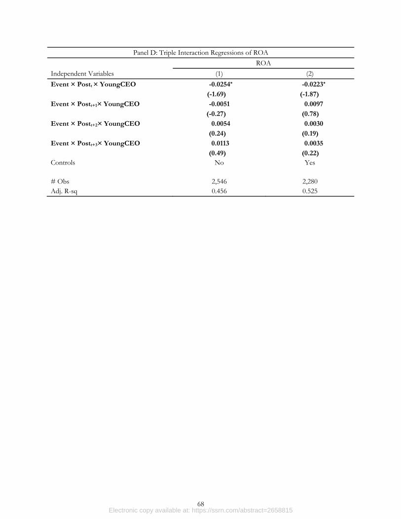
68

Panel D: Triple Interaction Regressions of ROA ROA

Independent Variables (1) (2)

Event × Postt × YoungCEO -0.0254* -0.0223* (-1.69) (-1.87)

Event × Postt+1× YoungCEO -0.0051 0.0097 (-0.27) (0.78)

Event × Postt+2× YoungCEO 0.0054 0.0030 (0.24) (0.19)

Event × Postt+3× YoungCEO 0.0113 0.0035 (0.49) (0.22)

Controls No Yes

# Obs 2,546 2,280 Adj. R-sq 0.456 0.525


Documents

Life is Too Short? Bereaved Managers and Investment Decisions