Do fund managers make informed asset

allocation decisions?

Bradyn Breon-Drish and Jacob S. Sagi

May, 2008∗

Abstract

We derive a model of dynamic asset allocation that allows us to infer whether, and

the degree to which, a portfolio manager is optimally using available information to

shift funds to and from equities. We test the model on a large dataset of mutual

fund holdings and find that the asset allocation decision of the typical mutual fund

manager, whether a professed market timer or not, is largely uninformed and fails to

incorporate public information into their asset allocation decision. We estimate that

this shortcoming can impose a cost on mutual fund investors of roughly 50-60 basis

points per year.

Keywords: Market timing, asset allocation, portfolio management, mutual funds.

Journal of Economic Literature Classification number: G14.

∗We thank Nick Bollen, Craig Lewis, and Hans Stoll for valuable discussions and comments. Researchsupport from the Financial Markets Research Center at Vanderbilt University is gratefully acknowledged.Bradyn Breon-Drish is at the Haas School of Business, UC Berkeley, 545 Student Services Bldg., Berkeley CA94720, Tel: 510-643-1423, email: breon@haas.berkeley.edu. Jacob S. Sagi is at the Owen Graduate Schoolof Management, Vanderbilt University, 401 21st Avenue South, Nashville, TN 37203, Tel: 615.343.9387,email: Jacob.Sagi@Owen.Vanderbilt.edu.

1

1. Introduction

Every active fund manager has to make asset allocation decisions, and changes in the portfolio

weights of major asset classes should be viewed as a function of the manager’s information

set and his or her ability to optimally use that information set. This paper develops a model

that can be employed to infer how much of a portfolio manager’s asset allocation decision

is made based on information and how much is uninformed. Uninformed asset allocation

decisions are those that needlessly incorporate noise, and our model enables us to quantify

the presence of such noise. We show that uninformed weight changes impose a cost on the

fund’s investors because they add uncompensated volatility to the fund’s returns. We then

apply the model to the portfolio weights of US mutual funds holding primarily US common

equity from 1979Q3 until 2006Q4. We find that, consistent with prior studies of timing over

holding horizons of a month or more, the asset allocation decisions of the typical mutual

fund manager exhibit an absence of both public and private information. Fund managers

whose explicit objective is to time the market fare no better. We estimate that the certainty

equivalent cost of making uninformed asset allocation decisions for an investor amounts to a

few basis points of the invested wealth per year. The opportunity costs of not using publicly

available information in asset allocation decisions is significantly greater at roughly 50 basis

points.

1.1. Motivation and literature review

The literature on portfolio management generally views ‘market timing’ as the shifting of

funds between broad asset categories (such as ‘US equities’, or ‘US Government bonds’) in

an attempt to capture higher risk-adjusted returns. Skillful market timers are said to divine

those times during which returns on one major asset class will exceed those of another. How-

ever, in contrast with successful stock-picking, some forms of market timing are theoretically

possible even in an informationally efficient market. Research over the past 20 years clearly

suggests that the equity premium and market Sharpe Ratio are predictable using well known

and easy to acquire public information, and that the application of this knowledge can pro-

1

vide additional value to investors, measured in terms of risk-adjusted returns, of about 1-2%

per year.1 Thus, at least in principle, one might expect market timing to be widely practiced

even if it is only based on public information.

1.1.1. Studies that do not support successful market timing

Most of the literature (e.g., Treynor and Mazuy, 1966; Henriksson and Merton, 1981; Pesaran

and Timmermann, 1994) focuses on a manager’s ability to shift resources between cash

and the US equity market, although recent studies also test for market timing ability with

respect to a broader range of asset classes. Despite the econometric issues that can arise in

testing fund returns for evidence of market timing (see Jagannathan and Korajczyk, 1986;

Ferson and Schadt, 1996; Edelen, 1999; Goetzmann, Ingersoll, and Ivkovic, 2000; Kothari

and Warner, 2001), most studies searching for timing ability have only examined returns,

largely concluding that active fund managers do not demonstrate better risk-return tradeoffs

via market timing over monthly or longer horizons.2 On the other hand, recent literature

directly analyzing fund holdings appears to conclusively indicate that professional active fund

managers exhibit significant skill in selecting individual securities (although their investors

do not generally benefit because of the fees and expenses charged by skilled managers).3 The

disparity between active managers’ ability to select individual securities and their inability

to deliver value through ‘market timing’ is especially puzzling given the research cited earlier

in support of the predictability of the market’s Sharpe Ratio.

1The predictability of market returns has been documented in Keim and Stambaugh (1986); Campbell andShiller (1988a,b); Breen, Glosten, and Jagannathan (1989); Lettau and Ludvigson (2001); Campbell (2002).The potential benefits from making use of this information in asset allocation decisions is documented in,among other papers, Kandel and Stambaugh (1996) and Whitelaw (1997).

2Studies finding no (or negative) evidence for timing include Treynor and Mazuy (1966); Henriksson andMerton (1981); Ferson and Schadt (1996); Graham and Harvey (1996); Wermers (2000); Kacperczyk, Sialm,and Zheng (2005); Kosowski, Timmermann, Wermers, and White (2006); Kacperczyk and Seru (2007).Daniel, Grinblatt, Titman, and Wermers (1997) search for ability in timing characteristics by looking atholdings. The papers that test market timing in multiple asset-allocation context include Daniel, Grinblatt,Titman, and Wermers (1997); Kacperczyk, Sialm, and Zheng (2005); Kosowski, Timmermann, Wermers,and White (2006); Kacperczyk and Seru (2007).

3See Daniel, Grinblatt, Titman, and Wermers (1997); Wermers (2000); Chen, Jegadeesh, and Wermers(2000); Cohen, Coval, and Pastor (2005); Kosowski, Timmermann, Wermers, and White (2006); Kacperczyk,Sialm, and Zheng (2005); Kacperczyk and Seru (2007).

2

1.1.2. Studies that do support successful market timing

There are several studies that find evidence of positive timing ability. In particular, the

consensus of studies that test fund returns for evidence of timing ability over daily horizons

appears favorable (Busse, 1999; Bollen and Busse, 2001; Chance and Hemler, 2001; Fleming,

Kirby, and Ostdiek, 2001). Such ability, however, likely has little to do with slower-moving

macroeconomic information shown to be useful for predicting returns at a much longer

horizon. Moreover, possessing the ability to time the market at the daily horizon does not

preclude the use of public information that forecasts the market at longer horizons. A more

promising study is Jiang, Yao, and Yu (2007) who estimate aggregate portfolio betas from

mutual fund holdings and find that funds tend to hold higher beta securities prior to when

market returns are high. Because they investigate timing ability using portfolio holdings,

their work is closest to ours.

1.1.3. Timing ability and funds’ equity holdings

The fact that active fund-managers are not generally deemed successful at market timing

does not appear to be for lack of trying. For instance, Figure 1 plots standardized values for

the consumption-wealth ratio variable (cay) constructed in Lettau and Ludvigson (2001), the

aggregate dividend ratio (dp), and the average domestic equity exposure (relative to their

sample mean) for funds identified as market-timers in our sample (an average of 27 funds each

quarter).4 Both cay and dp are thought to have forecasting power for the equity premium

(see Lettau and Ludvigson, 2001; Campbell, 2002), and over this period, the correlation of

cay, lagged one quarter, with excess return on the CRSP value-weighted index has been 17%,

which is significant at the 10% level. By contrast, equity exposures are far from significantly

correlated (ρ = −10%) with the market, and possess negative correlation with cay or dp

(−56% and −30%, respectively).5 Moreover, funds’ average equity exposure in our data

is significantly less persistent, indicating that the series is either considerably more noisy

4We describe in detail our method for classifying funds as market timers in Section 3 below.5Other variables that are thought to forecast the equity premium include the term spread and default

spread. The correlation of equity exposures with these variables is also weak.

3

than either cay or dp, or primarily contains high frequency information about changes in the

equity premium. Finally, when one multiplies the lagged change in equity exposure for each

fund by the market’s excess returns, then averages this quantity across funds and quarters

the result is a statistically and economically insignificant single basis point. Thus, if the

changes in equity exposure reflect an attempt to time the market over this period, then at

least at first blush, such efforts have not clearly translated into a valuable service.

On the other hand, cay and dp themselves are noisy predictors of the equity premium,

and if one naively uses asset allocation weights whose changes are proportional to cay, then

the average of ‘lagged weight changes × market returns’ is also statistically insignificant.

Moreover, weight changes ought to account for conditional volatility as well as conditional

means. Thus it is insufficient to consider Figure 1 in isolation as evidence against effective

asset allocation ability.

This sets up the research questions we investigate: To what degree do fund managers’

asset allocation decisions reflect information rather than noise, and to what extent can one

assess the cost to investors induced by purposeless asset-allocation? The second issue arises

for two reasons: Firstly, asset allocation that is largely noise can lead to utility loss to

investors because the random changes in weight induce spurious, and therefore uncompen-

sated, risk relative to an alternative policy.6 Secondly, by ignoring public information, fund

managers (and thus their investors) can miss an opportunity to enjoy higher Sharpe ratios.

We pose this question in relation to the asset allocation decision of any fund, not only those

that profess to be ‘market timers’.

1.2. Our contribution

In an attempt to shed additional light on these issues, this paper examines ‘market timing’

from several new perspectives. Firstly, consistent with the literature on the predictability

of aggregate returns, we assume that fund managers receive noisy signals about the market

Sharpe Ratio and accordingly adjust their portfolio weights. Such a strategy is known

6We establish this formally in the paper. Cox and Leland (2000) derive similar results.

4

to deliver value (Fleming, Kirby, and Ostdiek, 2001; Kandel and Stambaugh, 1996) when

the signal corresponds to public information. Our model augments this by considering

some degree of private information as well, potentially reflecting heterogeneity in the way

macroeconomic news is interpreted. Correspondingly, we characterize the Bayesian-optimal

changes in weights of a market timer who invests in the market or in short-term bonds, and

with a mean-variance myopic objective function, when he or she can condition on all past

information, and all past market returns.

Secondly, our theoretical analysis leads to some surprising results that easily lend them-

selves to empirical testing. The model predicts that the equity exposure of every portfolio

manager, whether they are market timers or not, ought to have an autocorrelation coefficient

similar to that of the time-varying equity premium. In particular, this autocorrelation ought

to be the same across funds regardless of their information structure. The intuition for this

result is simple: Say that the market’s conditional Sharpe Ratio is not directly observable but

is known to have a persistence characterized by an autocorrelation coefficient of φ. Because

all fund managers are using their information optimally to infer the market’s conditional

Sharpe Ratio, the time series of their best guess of it would also have an autocorrelation of

φ (otherwise, the fund manager would know that he or she has been systematically over- or

underestimating the conditional Sharpe Ratio). Given that portfolio market weights are es-

sentially proportional to the market’s Sharpe Ratio, the time series of market weights of any

fund that is optimally timing the market ought to have an autocorrelation of φ independent

of the fund’s identity.7

The model also predicts that a regression of market returns on lagged fund weights, with

appropriate controls, should result in a slope coefficient that is independent of the volatility

of the fund weights (i.e., the more the portfolio weight varies, the higher the forecasting

power). The intuition here is also simple. A large variation in portfolio weights reflects

better precision in forecasting the equity premium. The slope coefficient from a regression

7This is exactly true in a mean-variance portfolio allocation model where return volatility is constant.Our empirical tests adjust for the presence of time-varying return volatility and attempt to control for thepresence of non-myopic hedging demand.

5

of market returns on lagged fund weights is proportional to the correlation between weights

and returns, and inversely proportional to the volatility in weights. These two effects balance

each other, thereby leaving the slope coefficient constant.

A final prediction is that, because fund asset allocations reflect both public and private

information, they ought to predict returns at least as well as any variable constructed only

from public information.

These predictions should be robust because the economic rationale behind them tran-

scends the particular model we use. Nevertheless, the model used to derive these results

is rich in allowing a great deal of heterogeneity in fund managers and their private infor-

mation. We test the model predictions on a large panel of US mutual fund holdings, and

are able to, at least partially, assess the degree to which asset allocation decisions reflect

information as well as obtain rough estimates of the cost to investors induced by suboptimal

asset-allocation decisions. Our battery of empirical tests of the model’s predictions suggest

that, contrary to Jiang, Yao, and Yu (2007), little or no information is contained in funds’

asset allocation decisions.8 This appears to be robust to various econometric specifications

and holds up in the cross section and in the aggregate. Our most conservative estimate is

that 67% or more of the typical asset allocation decision is uninformed, and that there is

compelling evidence that fund managers, whether they profess to have timing ability or not,

appear to be neglecting valuable public information in their asset allocation decision. We

estimate, through a parametric model, that the combined certainty equivalent costs, due to

spurious asset allocation and neglect of public information, can amount to between 50 and

60 basis points of annual returns on invested wealth.

It is important, however, to temper our negative results by noting that the holdings

data used in our empirical tests are generally limited to US equity weights only. We have

no information on how funds invest outside of this asset class. Although our treatment of

fund holdings is consistent with that of other studies, these funds could in principal make

use of instruments such as index futures or high-yield bonds to change their effective equity

8Although we confirm the results of Jiang, Yao, and Yu (2007) for portfolio betas, we test and find thatthe equity portfolios generating these betas exhibit returns with no hint of timing ability.

6

exposure and our study would not pick this up.9 Moreover, it is also possible that the

reported poprtfolio holdings suffer from window dressing.

Section 2 develops the model. Section 3 describes our data set, the empirical methodol-

ogy, and reports our tests of the model. This section also compares our findings with the,

apparently contradictory, conclusions of Jiang, Yao, and Yu (2007). Section 4 estimates

the certainty equivalent costs of suboptimal asset allocation based on the empirical results.

Section 5 concludes.

2. A model of optimal market timing

We begin by considering a typical market-timing fund manager, identified by the index i,

who receives a noisy signal each period about the market risk premium and adjusts his port-

folio accordingly. Our assumptions represent a rich information environment, both across

managers and across time. Doing so enables us to achieve a level of realism and gener-

ality beyond the typical static modeling of the asset allocation decision under asymmetric

information.

The noisy signal received by manager i at date t is

sit = nit +mt, (1)

while the market’s excess return is assumed to be:

ret+1 = µ+mt + εt+1, (2)

where µ is the unconditional premium and mt is its time-varying component. Thus nit is the

noise component of the manager’s signal and the signal, sit, incorporates public information

(available to all fund managers) as well as private information.

The empirical literature notes that market return volatility is predictable. Consistent

9Almazan, Brown, Carlson, and Chapman (2004) document that few funds use derivatives.

7

with this, we assume that εt+1 has an observable date-t conditional variance of σ2εt.

10 We

also assume that the conditional variances of ut and vit are constant and denoted as σ2u and

σ2v , respectively. We further assume that

mt = (1− φm)mt−1 + ut,

nit = (1− φin)nit−1 + vit,

such that each shock in the collection, { εsσεs−1

, usσu, visσiv}s≤t is a standard normal iid random

variable, independent of the process that generates σ2εt. Under our assumptions, mt and

σ2εt are independent and universal to all managers while nit may or may not be correlated

across managers.11 Moreover, the variance of noise in managers’ signals is heterogeneous in

precision as well as persistence.

Under our assumptions, Var[mt] = σ2u

1−(1−φm)2and Var[nit] =

σ2iv

1−(1−φin)2; we’ll refer to these

unconditional variances as Var[m] and Var[ni], respectively. Let Iit correspond to manager

i’s information set, consisting of observations of six, σ2εx and reix for all dates x ≤ t. Finally,

we assume that the manager seeks to myopically maximize a mean-variance function of his

portfolio returns, implying that the optimal allocation at date t is

wit = Aiµ+ E[mt|Iit]

σ2εt + Var[mt|Iit]

. (3)

The proportionality factor, A, can be viewed as a measure of relative risk tolerance and

is assumed constant through time. Thus, if σm = m0 = 0 and σ2εt is constant (i.e., there

10It appears realistic to assume that investors observe the conditional volatility of market returns (using,for example, the S&P500 volatility index). In other words, Var[ret+1|Pt] is observable, with Pt representing acommon knowledge (public) information set. Under the assumption that mt is independent of εt+1, assumingthe observability of σ2

εt presupposes that Var[mt+1|Pt] is separately observable.11Without loss of generality and without changing our main results, one can replace µ with ξσ2

εt plusa constant, consistent with various asset pricing models. Various studies explore the relationship betweenthe market’s conditional variance and expected returns. Whitelaw (1994) demonstrates that the theoreticalrelationship may not be monotonic, French, Schwert, and Stambaugh (1987) find a positive relationshipwhile Breen, Glosten, and Jagannathan (1989) and Breen, Glosten, and Jagannathan (1989) do not. In lightof this, we elected not to explicitly model such a relationship, although we account for its potential presencein the empirical section

8

is no predictability in the market’s Sharpe Ratio), then the manager follows a strategy of

rebalancing to constant weights. When we test the model, we revisit this assumption and

control for alternative specifications that are consistent with dynamic portfolio management

for an optimizing agent (e.g., a buy and hold strategy, or a portfolio insurance strategy).

Assuming a mean-variance objective function is consistent with the preferences of a log-

investor who can rebalance continuously, but the assumption ignores the additional hedging

demands of other types of investors. In neglecting a hedging demand component, we note

that its sign and magnitude vary with investor preferences and horizon, while all investors

place some (often considerable) weight on the myopic allocation given by Eq. (3).12 Finally,

we note that, to the extent that the equity premium affects the expected returns of all stocks,

Eq. (3) ought to apply to all managers of equity portfolios (i.e., both ‘stock pickers’ and

‘market timers’).

The following proposition establishes properties of the manager’s optimal forecast of the

time-varying component of the equity premium.

Proposition 1.

mit ≡ E[mt|Iit] =

(∞∑j=0

aitjsit−j +∞∑j=0

bitj(ret−j − µ)

), (4)

where the coefficients {aitj, bitj}∞j=0 provide a solution to the following infinite set of linear

12Kim and Omberg (1996) and Wachter (2002) demonstrate that when the Sharpe Ratio is an AR(1)process in continuous time, any investor who can rebalance continuously and has utility over terminal wealthwith constant relative risk aversion will allocate her wealth to equities by modifying Eq. (3) to includecalendar-time dependence in A and an additional calendar-time dependent constant. Detemple, Garcia, andRindisbacher (2003) find that variations in the hedging demand are significantly less pronounced than thoseof the myopic solution. Overall, this suggests that Eq. (3) captures much of the information content inchanges to equity allocations even in the presence of a hedging demand.

9

equations:

(1− φm)kVar[m] =∞∑j=0

aijt

(Var[m](1− φm)|k−j| + Var[ni](1− φin)|k−j|

)+∞∑j=0

bijtVar[m](1− φm)|k−j−1|, k ≥ 0

(1− φm)k+1Var[m] = biktσ2εt−k−1 +

∞∑j=0

aijtVar[m](1− φm)|k+1−j| +∞∑j=0

bijtVar[m](1− φm)|k−j|, k ≥ 0.

Moreover,

Var[mt|Iit] = σ2εt−1(1− φin)bi0t + Var[ni]ai0tφin(2− φin). (5)

Proofs to all results are found in Appendix A. Although being able to actually solve

the infinite set of equations in Proposition 1 is not germane to our analysis in this paper,

it is worth noting that the infinite set of coefficients in Proposition 1 can be approximated

extremely well by truncating the higher order equations. In numerically experimenting with

the equations, we’ve found that for realistic parameter settings it suffices to keep only those

coefficients for which k ≤ 5.

2.1. Testable predictions

The next result is central to the empirical tests we develop.

Proposition 2. The unconditional autocorrelation of mit is 1 − φm, coinciding with the

unconditional autocorrelation of mt.

Thus, controlling for the denominator in (3) (say, by multiplying wit by σ2εt and assuming

σ2εt � Var[mt|Iit]), the autocorrelation of the optimal weight assigned to the market is the

same across managers despite the rich heterogeneity in managers’ information structure.

One can understand the intuition for the result as follows: Every manager knows that the

conditional equity premium has persistence of (1−φm). If her estimate of the equity premium,

10

mit, exhibits a different level of persistence, then the manager is either over-reacting or under-

reacting to new information.

A second result that is key to our empirical tests relies on the observation that, controlling

for the denominator in (3), the variation in weight is related to the quality of the manager’s

signal. If the quality of the signal is poor (i.e., Var[m]Var[m]+Var[ni]

is small), then the manager will

optimally react by being careful not to make dramatic changes in the weights, which are

proportional to changes in E[mt|Iit]. Likewise, a high quality signal will be associated with

larger shifts in weights in response to the signal. Thus, a higher variance of portfolio weights

ought to reflect better forecasting power for the market returns. This is the subject of the

next result.

Proposition 3. The regression of ret+1 on mit yields a slope coefficient of β = 1, and the

unconditional correlation of ret+1 with E[mt|Iit] is ρrmi =σmiσr

, where σr is the unconditional

standard deviation of equity returns and σmi is the unconditional standard deviation of mit.

In particular, controlling for the conditional volatility (again, by multiplying wit by σ2εt

and assuming σ2εt � Var[mt|Iit]), the slope coefficient in a regression of market returns

on lagged weights ought to be proportional to 1Ai

— which in turn is related to the average

unconditional portfolio weight. Given that the data allows one to estimate the latter quantity,

this is essentially how we will test Proposition 3.

2.2. Suboptimal asset allocation

In this section we establish that it is inadvisable for a portfolio manager to make uninformed

asset allocation decisions. By an ‘uninformed asset allocation decision’ we refer to changes

in portfolio weights that are not contingent on past or present return-relevant variables (e.g.,

the tossing of a coin).

Because it is easier to make our point in a continuous-time setting, we consider a filtration

generated by multi-dimensional Brownian motion, and corresponding to the information set

of the manager. Suppose that the continuous-time random variables, rft, µet, σet, w∗t , ret

and ηt are adapted to the filtration and that ηt is independent of the other variables and

11

has an unconditional mean of zero. Interpret rft as the instantaneous risk-free rate, µet

and σet are, respectively, the optimal estimates of the instantaneous market risk premium

and the instantaneous market return volatility based on the manager’s information, ret is

the realized market excess return, and w∗t corresponds to a set of weights adapted to the

filtration generated by {rft, µet, σet, ret}. Suppose that the manager chooses wt ≡ w∗t + ηt to

be the portfolio weight. An investor who invests with the manager over the horizon [0, T ]

will see his wealth grow from W0 at time 0 to WT at time T and given by

WT = W0 exp(∫ T

0

(rft + wtµet −

1

2σ2etw

2t

)dt +

∫ T

0

wtσetdBt

), (6)

where dBt is an infinitesimal Brownian increment that is adapted to the filtration generated

by {rft, µet, σet, ret}. In what follows, we only consider investors with utility over date-T

wealth, neglecting consumption or income considerations.13

Proposition 4. Any investor with utility only over date-T wealth who is at least as risk-

averse as a log-investor will strictly prefer that the manager use the investment policy w∗t

rather than wt. Moreover, the certainty equivalent loss for such an investor, measured in

terms of an annual fee on managed wealth, is at least

f =1

2TE[ ∫ T

0

η2t σ

2etdt]. (7)

It is worth emphasizing that the certainty equivalent cost in Eq. (7) is assessed relative

to any policy w∗t . In particular, the expression does not incorporate the lost opportunity cost

of failing to take advantage of the predictability in expected returns. We assess the latter in

Section 4.

13It is tedious, though not hard, to extend the results here to the case where the investor consumes fromsavings and/or makes periodic contributions from labor income.

12

3. Empirical investigation

Our empirical work is guided by the model results of Section 2.1 where it is assumed that

the portfolio weight assigned to the market are given by Eq. (3). Before we can apply the

results of the model to open-end mutual funds holding domestic equity, we have to address

two issues. First, funds may not follow a strategy that rebalances to constant weights in

the absence of information (i.e., time-varying Sharpe Ratios). One example of this is a buy-

and-hold strategy, while another is portfolio insurance. In the case of iid returns, it is well

known (e.g., Cox and Leland, 2000; Leland, 1980) that these three dynamic strategic do not

dominate each other in the sense that certain investors (e.g., those exhibiting a particular

version of decreasing relative risk aversion) might prefer portfolio insurance while others

might prefer a rebalancing strategy. Moreover, in the presence of trading costs, it may be

optimal to allow weights to wander within an ‘inaction’ region (see Davis and Norman, 1990)

and the optimal allocation of new funds might therefore exhibit a lag. Because all of these

alternative reasons for weight changes are contingent on past returns or fund flows, which

are orthogonal to the error term in forecasting mt, one can still test the model by controlling

for past returns and fund flows.

Second, the Propositions pertain to the numerator of Eq. (3), whereas in practice portfo-

lio weights incorporate the denominator as well. Thus, in testing whether asset allocation is

informed, one must control for the conditional volatility. This can be done using a volatility

index such as the vix, acknowledging that such a market forecast of volatility will differ,

though likely not by much, from the manager’s own volatility forecast.14

Recapping the insights from Section 2, controlling for the conditional market volatility,

1. The autocorrelation of weights allocated to equity should be the same across funds.

2. A regression of market returns against lagged portfolio weights allocated to equity

ought to yield a positive slope coefficient inversely proportional to the average uncon-

14The difference between Var[ret+1|Pt], where Pt represents a common knowledge (public) information set,and Var[ret+1|Iit] amounts to the difference between Var[mt+1|Pt] and Var[mt+1|Iit], which ought to be smallrelative to σ2

εt.

13

ditional portfolio weight.

3. mit, and therefore a fund’s equity weight, ought to forecast the equity premium at least

as well as publicly available variable. Moreover, one would anticipate that it should

be positively correlated with macroeconomic variables that predict the conditional

market’s Sharpe Ratio.

3.1. Data

We obtain quarterly holdings information for all mutual funds, from 1979Q3 until 2006Q4,

in the Thompson Financial CDA/Spectrum s12 database accessed through the Wharton Re-

search Data Services (WRDS). The data is then linked to CRSP through WRDS’ MFLinks

service and the CRSP survivorship bias-free Mutual Fund Database (MFDB). For each quar-

ter and each fund we obtain, whenever available, the portfolio weight corresponding to the

total domestic equity holdings of the fund, the value-weighted return on those holdings in the

three months immediately following the report date, the S&P objective, style and specialty

fund codes (from CRSP MFDB), and the CDA/Spectrum s12 investment objective fund

code.15 We also obtain the return to fund investors, net of distributions, for each calendar

quarter and document the dollar value of total assets managed by the fund. We augment

this with quarterly data constructed from the monthly series of CRSP value-weighted returns

and the risk-free rate (from WRDS), and quarterly data for the aggregate dividend yield and

earnings-to-price ratio on the S&P500 index (Global Financial Data). Finally, we compute

three different predictors of market volatilities: the first predictor is a naive monthly volatil-

ity calculated using the past month’s daily CRSP value-weighted return data, the second

corresponds to a fit of monthly CRSP value-weighted return data over the period 1954-2006

to a GARCH(1,3) model, and the third consists of the S&P100 volatility index (vxo from

15Because funds report their holdings at different times, the holding returns are not contemporaneousacross all funds. When a fund reports holdings more than once in a quarter, we consider only the earliestreport for that quarter. Many funds only report twice a year, the minimum SEC requirement, resulting insubstantial ‘seasonality’ in the number of funds that report each quarter.

14

WRDS).16 In merging this data with our quarterly observations, we choose the volatility

predictor for the last month of each quarter.17

We initially start with 5278 funds. We filter out funds that at any point reported an

equity portfolio weight of more than 200% (76 funds), funds that report holdings in fewer

than eight quarters (983 more funds), and funds with an average equity portfolio weight of

less than 50% (774 additional funds). We generally wish to investigate funds that invest in

a broad enough range of domestic equity so that information about the US equity premium

ought to particularly matter to them. Table 2 tabulates how the remaining 3445 funds are

then categorized as ‘broad domestic equity funds’ using their CDA/Spectrum s12 investment

objective codes, ICDI (MFDB) objective codes, and S&P objective codes.18 Funds not

highlighted in the table are considered ‘broad domestic equity funds’. We exclude the other

funds from the sample and are left with 2766 funds. Even for these remaining funds, some

fields are missing for some (or all) quarters.

For each fund, we calculate the time-series average weight of domestic equity in the

fund’s portfolio, the average total net assets under management, the number of observations,

the contemporaneous correlation of returns on the fund’s domestic equity portfolio with

the CRSP value-weighted index returns, the contemporaneous correlation between a fund’s

domestic equity portfolio weight and the various predictors of market return variance. We

also calculate the correlation between the domestic equity portfolio weights of every pair

16We found the GARCH(1,3) model to be the most parsimonious best fit nested within a GARCH(4,4)framework. Of the three, the GARCH measure is the only one that is incorporates information unavail-able contemporaneously because the coefficient estimates use the full time series. This turns out to beinconsequential for our tests.

17For the GARCH measure of volatility, while we could have used an average of the forecast for all threemonths of the quarter based on the last quarter’s information, this doesn’t significantly impact our testresults. Moreover, weights are typically reported towards the end of the quarter and would therefore reflecta volatility prediction for that month (given that turnover ratios for the average mutual fund tend to belarger than what might be suggested from reported quarterly weight changes).

18Some funds change objective codes throughout the sample period. We assign a fund its modal investmentcode, and when there is more than one mode, we assign the ‘largest’ one (numerically or alphabetically).In classifying a fund, we rely firstly on its CDA/Spectrum s12 objective code and consider it not to be abroad domestic equity fund if the investment code is 1 (‘International’), 5 (‘Municipal Bonds’), 6 (‘Bond andPreferred’), or 8 (‘Metals’). Only 2289 of the 3445 funds surviving the initial filter have a CDA/Spectrums12 objective code. Surprisingly, 170 funds have an investment code of 1, 5, 6, or 8, meaning that, despitetheir objective, they mostly hold U.S. domestic equity (150 of these are classified as ‘International’). Noneof the unclassified funds have an entry for their MFDB policy code or Wiesenberger objective.

15

of funds in our sample that have at least eight overlapping weight data (2,677,052 pairs).

Finally, we compute the CAPM β and α for the fund’s domestic equity returns, the t-statistic

for the α, and the Sharpe Ratio of the non-CAPM returns (i.e., the α divided by the standard

deviation of the CAPM regression residual, or the ‘information ratio’). Table 3 provides a

summary of these statistics across funds.

The summary statistics indicate that the funds in our sample maintain a high average

portfolio weight in equities, and that it is not unusual for this weight to fluctuate by 10% or

more each quarter. Moreover, the equity portfolio held by the typical fund is highly correlated

with the market portfolio (this is also confirmed by CAPM β of the equity portfolio held

by the typical fund). Thus, even those managers who do not confess to have special timing

ability could benefit from timing based on public information. A surprising fact is that the

average fund slightly increases its weight in equities when market volatility is predicted to

be high. This would be inconsistent with Eq. (3) and the basic objective of maximizing

a fund’s Sharpe Ratio even if the equity premium is proportional to the market variance.

Another striking statistic is the low typical correlation between the equity weights of any two

funds. This suggests that much of the asset allocation taking place is largely due to noise.

Overall, the typical fund in our sample is not particularly good at picking stocks either,

although according to Kosowski, Timmermann, Wermers, and White (2006) it is likely that

the highest ranked funds do exhibit ability.

Of the 2766 funds we examine, we classify as ‘timers’ those funds that (i) explicitly

specify flexibility or dynamic asset allocation in their MFDB policy code, S&P objective

code, S&P style code, or S&P specialist code; and (ii) have a time-series standard deviation

greater than 0.067 for portfolio weight allocated to domestic equity.19 We list the names

of the 54 funds classified as ‘timers’ in Table 4, and provide summary statistics in Table 5.

The ‘timers’ tend, on average, to commit less money to equities and their equity portfolio

is more highly correlated with the market. While they have a lower correlation with market

19We select 0.067 because this is the median standard deviation of weights for funds in our sample. Thereason we add this minimum standard deviation requirement is because managers who are skilled at assetallocation ought to exhibit greater changes in portfolio weights than their counterparts.

16

volatility predictors, the typical pair-wise correlation among them is comparable to that in

the unconditional sample.

3.2. Testing Proposition 2

We begin by examining the degree to which the dynamics of the weight allocated to equities

is similar across funds, consistent with Proposition 2. In order to control for strategy and

for time-varying volatility, we posit that the fund’s weight in equity can be written as

wit = Aimit

σ2it

+Bi + γi1rit−1 + γi2r2it−1 + δifit, (8)

where rit−1 is the excess return on the fund’s equity, fit is fund’s growth in net assets due

to net inflows, and Bi is a constant.20 By including rit−1 and r2it−1 we are controlling for

persistent changes in weights due to strategies such as buy-and-hold or portfolio insurance.

These terms, along with fit, also control for the presence of ‘no trade’ regions that arise in

the presence of transaction costs or other forms of illiquidity. Assuming that σ2εt+Var[mt|Iit]

can be approximated with a predictor of market variance, say σ2p t (e.g., σ2

vox t), one can use

the result from Proposition 2 to rewrite Eq. (8) as the following regression equation:21

σ2p t+1wit+1 =(1− φm)σ2

p twt + γi1σ2p t+1rit + L.γi1σ

2p trit−1 + γi2σ

2p t+1r

2it + L.γi2σ

2p tr

2it−1

+ δiσ2p t+1fit+1 + L.δiσ

2p tfit + εit+1 + τiσ

2p t+1 + L.τiσ

2p t + consti, (9)

Ifσ2p t

σ2εt+Var[mt|Iit]

is constant, then the residual εit+1 is uncorrelated with all other variables on

the right side of Eq. 9 (this follows from Proposition 2 and the Law of Iterated Expecta-

tions). Thus 1 − φm can be estimated through ordinary least squares (OLS). Likewise, it

is straight forward to demonstrate that εit+1 is correlated with rit+1. Thus, had we used

contemporaneous returns to control for strategy, we would not be able to estimate 1 − φm20If, as discussed in footnote 11, the predictable part of the equity premium includes a term such as ξσ2

p t,then by including the constant Bi we ensure that mit accounts for other predictive variables.

21In Eq. (9), each coefficient named L.x should, in principle, be proportional to the coefficient x. Whentesting the regression, however, we allow these identified coefficients to be free because no estimation bias isintroduced by doing so.

17

via OLS. In practice,σ2p t

σ2εt+Var[mt|Iit]

is unlikely to be constant. If its variation is small, then

the consequent error-in-variables problem will not be serious. If the variation is large, then

the bias in the estimate of 1 − φ is likely to be large. We therefore use various methods to

estimate Eq. (9).22

To test the hypothesis that 1 − φm estimated via OLS is the same across funds we

first perform the mixed-effects regression indicated in Eq. (9), assuming that residuals are

heteroskedastic but uncorrelated across funds.23 While this assumption is questionable, we

are reassured by the fact that, as indicated in Table 3, the average cross-sectional correlation

among the dependent variables (the equity weights) is low. Table 6 reports cross-sectional

averages for the mixed panel regression under different assumptions for σ2p t, for the entire

sample of funds as well as for the sample of timers. It is evident that including some

of the control variables is important while others are unimportant. For the most part,

one can conclude that funds follow a strategy of rebalancing to constant weight with a

negative response to flow, suggesting the presence of some lag in moving new funds (which

are most likely to be cash) to the optimum allocation. Using the GARCH predictor for

market volatility yields the highest autocorrelation, at 0.436. Timers have a significantly

higher autocorrelation. For comparison, in our sample, the autocorrelations of cay, ep, and

dp are 0.89, 0.97, and 0.98, respectively, and of the three, cay is the best predictor of returns.

The last line of Table 6 gives the result of a likelihood ratio test relative to a model that

fixes the autocorrelation coefficient across funds. Across the board, one can strongly reject

the hypothesis that funds share the same autocorrelation coefficient. Thus, our test of

Proposition 2 is rejected. Moreover, the measured autocorrelation is significantly lower than

what might be expected from a predictor of expected returns.24

To test the robustness of the conclusions from the mixed-effects regression reported in

22We attempted to use ret+1 as an instrument because, theoretically, it is unconditionally correlated withmit and empirically unrelated to the other variables. In practice, however, the poor signal to noise in realizedreturns resulted in meaningless results.

23Fund flows are calculated as the difference between the growth in net assets under management less thegrowth in NAV per share. We drop observations for which the flow is less than -100% and more than 200%(269 out of 61251 instances where flow data was available).

24An alternative hypothesis is that funds make use of higher frequency information about expected returns.This is unlikely, given the lack of forecasting power in the weights (on which we report later).

18

Table 6, we also separately estimate the coefficients in Eq. (9) and calculate the statistic

C =1

N

N∑i=1

(φm − φi)2

se2φi

, (10)

where N is the number of funds, 1 − φi is the estimate of the autocorrelation coefficient

from the ith regression and seφi is its standard error. φm is taken to be the GLS estimator

of the mean of the φi’s (i.e., φm =∑i φi/se

2φi∑

i 1/se2φi

). Given the large number of funds and the

fact that the weights are not highly correlated, and as long as the GLS estimator has a

standard error much less than 1, C should be approximately normal with mean and standard

deviation of 1 under the null. Table 7 reports the value of 1 − φm, the test statistic C,

and its p-value under the null for the full sample, for the timers only, and using various

proxies for the conditional volatility.25 We report the estimation result imposing various

filters for the minimum number of observations in a fund to mitigate the potential adverse

impact of small sample distributions on the estimator φi. It appears that, by and large, the

results are consistent with those in Table 6 and robust to small samples issues. The fact

that the allocation persistence of short-lived funds in the unconditional sample is different

from that of long-lived funds comes as a surprise given that Carhart (1997) and Kosowski,

Timmermann, Wermers, and White (2006) find no difference in their relative performance.

3.3. Testing Proposition 3

Consider the following regression

ret+1 = ζiσ2ptwit + γi1σ

2ptrit−1 + γi2σ

2ptr

2it−1 + δiσ

2ptfit + τiσ

2pt + εit+1 + consti. (11)

Under our assumption, Eq. (8), σ2p twit corresponds to σ2

pt times the sum of the control

variables, plus Aimit. Moreover, under the null the forecast error in mt is orthogonal to the

control variables in the equation, thus averaged across funds ζ in the regression equation

25If the φi’s are highly correlated, C would resemble a χ2 distribution. Even in this unlikely situation, thehypothesis that φi is the same across funds is solidly rejected at the 10% level across the board.

19

(11) should be positive and, according to Proposition 3 and Eq. (3), roughly equal to 1Ai

.

Assuming µ > 0.01 (quarterly), that the unconditional quarterly market volatility is lower

than 0.10, and that the typical equity weight of a fund in our sample is less than 1.0, one

can deduce a lower bound on ζ of 1Ai> 0.01

1.0×0.12 = 1.0. Using sample means for µ, the market

volatility, and average weights, one deduces a value closer to 1Ai≈ 3. A distribution of

ζi’s with mass significantly below 1 implies that weight changes in our sample of funds are

suboptimal and incorporate an uninformed component.26

For each fund, we estimate ζi in Eq. (11) via an OLS regression. The assumption that

ζi > 1 implies that ζise(ζ)

> 1se(ζ)

. By summing across funds, and assuming that the estimate

ζi is normally distributed with variance se2(ζ), we arrive at 1N

∑i

(ζi

se(ζ)− 1

se(ζ)

)> E , where E

is the average of N correlated standard normal distributions. The correlation arises because

the same dependent variable is used in each regression, thus the cross-sectional correlation

between the errors of the estimates is the cross-sectional correlation between the mit’s. If N

is large, E is normally distributed with variance equal to the average correlation among the

mit’s. We approximate this average correlation to equal 0.08, consistent with the average

correlation between the weights as documented in Tables 3 and 5. Table 8 reports average

values of the ζi’s, the probability that 1N

∑i

(ζi

se(ζ)− 1

se(ζ)

)> E under the null, and the

probability that 1N

∑i

(ζi

se(ζ)− 2

se(ζ)

)> E under the null. The results suggest that the typical

fund exhibits weight variation that is uninformed. In particular, the average ζi is well below

its expected value of about 3, and even below the conservative lower bound of 1. If ζ is a

fraction, say x, of what it should be, then x is also the fraction of the informed (i.e., optimal)

variance over total variance of the fund’s weight changes. I.e., x = Var[mt|Iit]Var[mt|Iit]+π2 , where π2 is

the variance component in weight changes that is uninformative in the sense that, given Iit,

it contains no information about future returns.

Table 8 implies that the population value of ζ is likely to be a fraction of 1. Given that

the expected value of ζ based on optimal use of information is around 3, it appears that

26Alternatively, one can attribute a lower coefficient to an error-in-variables problem. The error-in-variableproblem ought to equally affect the results in Tables 6 and 7. The results there suggest that this is not thesource of the problem.

20

67% or more of the changes in asset allocation made by the typical fund are uninformed and

suboptimal from our model’s perspective.

3.3.1. Robustness

To confirm this negative result, we test, using a bootstrapping methodology, whether the

cross-sectional distribution of ζi’s in the regression equation (11) is different than what would

arise under the null of ζi = 0 for all i. The methodology proceeds as follows:

1. Using the data, the regression equation (11) is estimated for each fund, and the t-

statistics for ζi, denoted as ti, is saved along with the corresponding regression residual.

Because the residuals in our model are heteroskedastic, White (1980) standard errors

are used when computing t-statistics.

2. Next, the regression equation (11) with ζi set to zero is estimated:

ret+1 = γi1σ2ptrit−1 + γi2σ

2ptr

2it−1 + δiσ

2ptfit + τiσ

2pt + εit+1 + consti,

and the predicted returns, reit+1 ≡ ret+1 − εit+1 are saved.

3. The set of dates {1979Q3, . . . 2006Q4} is randomly sampled, with replacement, to cre-

ate 2000 sets of data, each of which has the same time-series length as the original sam-

ple. Denote by T (k, t) the random element from {1979Q3, . . . 2006Q4} corresponding

to the tth item in the kth sample.

4. For each fund, we construct 2000 sets of bootstrapped sample returns under the null

that ζi = 0 by combining randomly drawn residuals from the unrestricted model in

step 1 with the predicted returns from step 2. Specifically, the return at date t of the

kth bootstrapped sample is:

reikt∗ = reit + εiT (k,t).

21

This approach preserves the cross-sectional properties of the residuals in each of the

2000 bootstrapped panels.

5. For each fund, denoted by i, and bootstrapped sample, denoted by k, the following

time-series regression is estimated:

reikt+1∗ = ζ∗ikσ

2ptwit + γ∗ik1σ

2ptrit−1 + γ∗ik2σ

2ptr

2it−1 + δ∗ikσ

2ptfit + τ ∗ikσ

2pt + ε∗ikt+1 + const∗ik.

The estimate for the t-statistic associated with each ζ∗ik is saved. This exercise essen-

tially samples the joint distribution of the t∗i ’s, the t-statistics associated with the ζi’s,

under the null of no timing ability. For the kth bootstrapped panel, let Γk(`) denote

the cross-sectional `th percentile of among the t∗i ’s.

6. The one-sided p-values for the cross-sectional percentiles, Γ(`), of ti’s from step 1 are

computed according to

p(`) =1

2000

2000∑k=1

1{Γk(`) > Γ(`)},

For instance, p(50) corresponds to the likelihood, under the null, that we would observe

by chance alone a sample median ti as high or higher than the median ti in step 1.

In particular, if p(50) is small, then this could be interpreted as evidence that the

asset allocation decisions made by the median manager contain more information than

would be expected under the null.

Table 9 reports various cross-section percentiles of ti’s when the regression is performed

using our three different measures of market volatility and when various restrictions are

imposed on funds’ age in the panel. The bootstrapped p-values are reported below each

estimated percentile. Fpr virtually all values of `, Γ(`) is not significantly greater than

what is obtained under the null that ζi = 0. There is no evidence that the cross sectional

distribution of ζi’s is shifted to the right of what would expected under a null of ζi = 0. Thus,

consistent with the previous test, fund managers, including those with significant values of

22

ti, do not appear to move portfolio weights between equity and non-equity in a manner that

predicts future market returns.27

3.3.2. Interpreting the negative results in light of Jiang, Yao, and Yu (2007)

Jiang, Yao, and Yu (2007) report that lagged equity portfolio betas of open-end mutual funds

predict market returns. Specifically, fund managers appear to be holding equity portfolios

with higher betas prior to positive market outcomes, and tend to be in possession of equity

portfolios with lower betas prior to negative market outcomes. This is viewed as supportive

of timing ability on the part of active fund managers. Appendix B qualitatively confirms

that, in our sample, equity portfolio betas also predict market returns. Our results differ

somewhat from those of Jiang, Yao, and Yu (2007) (see their Table 3) in that we find no

evidence of predictability at the 1- and 3-month horizon, whereas Jiang, Yao, and Yu (2007)

do find such evidence at the 3-month horizon.

There are several ways to rationalize this with the negative results of the previous subsec-

tion. It might be the case that the vast majority of market timing efforts exerted by managers

could be directed towards reallocating equity into or out of higher beta stocks rather than

shifting weight from non-equities into or out of equities.28 Alternatively, it might be that

the Jiang, Yao, and Yu (2007) finding is not actually reflective of market timing ability,

perhaps because of mis-measurement in the portfolio betas, because the shift into higher

(lower) beta portfolios is accompanied by a shift into lower (higher) non-market systematic

risk, or because changes in funds’ equity portfolios might be taking place at a frequency that

is too high to benefit from the predictability at 6- to 12-months’ horizon.

To help shed light on whether the holdings-based predictability is indicative of market

timing ability, we perform Treynor-Matzuy (TM) and Henriksson-Merton (HM) regressions

on the cross section of funds’ equity portfolio returns and compare the standardized timing

27We reached the same conclusions when we repeated the bootstrapping exercise using the Kosowski, Tim-mermann, Wermers, and White (2006) approach. Moreover, the bootstrapping procedure yields significantlypositive results in a simulated sample of weights that do have weak predictive power for the equity premium.Thus the lack of evidence is unlikely to be because of a lack of power.

28If a significant minority of funds timed the market via asset allocation and the remainder did not, thenone would still expect to find weak, though supportive, evidence for market timing in our test.

23

coefficients from these regressions with those from bootstrapped samples for which, by con-

struction, there is no timing ability. Jiang, Yao, and Yu (2007) examine TM and HM return

regressions for fund returns, although these suffer from the fact that the fund-level returns do

not reflect the equity portfolio returns because the former result from trading at a frequency

greater than quarterly and trading in assets other than equities. By contrast, we look at the

results of TM and HM bootstrapped tests for the same portfolios whose market betas are

shown to exhibit predictive power. Because the rebalancing period for these portfolios coin-

cides with the observation frequency by construction, the criticism of Goetzmann, Ingersoll,

and Ivkovic (2000) and Jagannathan and Korajczyk (1986) do not apply to our tests.

We performed two bootstrapping procedures to assess the significance of the TM and

HM timing regressions. The first procedure proceeds similar to Bollen and Busse (2001) and

attempts to obtain correct standard errors for the TM and HM timing coefficients. Using

quarterly data, the regression

reit = consti +∑

j∈{m,smb,hml,umd}

βjrejt + γif(remt) + εit, (12)

is run for each fund, where reit is the excess return on the equity portion of the fund’s

portfolio, rekt is the return for Fama-French-Carhart factor k, and f(remt) = (remt)2 for

the TM model and f(remt) = 1{remt > 0}remt for the HM model. The fitted values, reit ≡

consti +∑

j∈{m,smb,hml,umd} βjrejt + γif(remt) and the residuals are saved. We next create 2000

bootstrapped panels as follows. To create a single bootstrapped panel the set of dates is ran-

domly resampled, with replacement, and the residuals for each fund reordered accordingly.

Then, the resampled residuals are merged back with the rit’s, producing a time-series panel

of pseudo-return data for the funds’ equity portfolios. The equity portfolio pseudo-returns

for a given fund is considered missing if no residual is available for the resampled date. The

regression in (12) is re-run for each replication of each fund. The bootstrapped standard

24

error of each estimated γi parameter is computed using

Std. Err.(γi) =1

2000− 1

2000∑k=1

(γik − γik)2 .

t-statistics are computed using the formula

t =γi

Std. Err.(γi),

and are compared to ±1.96 to assess significance. For consistency with the Jiang, Yao, and

Yu (2007) replication results, we require a fund have a minimum of 8 quarters of data to

qualify for inclusion in the sample. Panel A of Table 10 shows the results for this procedure

and is analogous to Table III in Bollen and Busse (2001). The fact that the number and

magnitude of negative and positive timing coefficients is roughly the same suggests that there

is no serious negative bias of the sort suggested in Jagannathan and Korajczyk (1986) and

Goetzmann, Ingersoll, and Ivkovic (2000), and found in the analysis of fund-level returns by

Jiang, Yao, and Yu (2007). The fact that highly significant coefficients are no more frequent

than might be expected is evidence against timing ability, as reflected in equity portfolio

returns.

A potential shortcoming of the test just reported is that the t-statistics might not be

t-distributed, and thus inference of significance through a critical score of 1.96 might not be

appropriate. Our second bootstrapping procedure, similar to the procedure used to test the

timing regression in Section 3.3.1, is aimed at addressing this. We proceed similarly to the

method outlined above except that reit is now defined as reit ≡ consti+∑

j∈{m,smb,hml,umd} βjrejt,

and the pseudo returns are generated by combining rit with reordered values of εiT (k,t), where

T (k, t) is defined as in Section 3.3.1. The timing regression is then re-run for each replication

of each fund, and right-tail p-values are calculated for various percentiles, as in Section 3.3.1.

The results, reported in Panels B and C of Table 10, confirm those from Panel A sug-

gesting that there is no evidence of timing ability in funds’ equity portfolios.

To recap, although the equity portfolios of actively managed funds, as reconstructed

25

from quarterly holdings, exhibit portfolio betas that predict market returns at a horizon of 6

months or greater, we find no evidence that this translates into successful timing as measured

in terms of quarterly portfolio returns. This could be because the portfolios are not held

long enough to benefit from the predictability. Alternatively, this could be because of mis-

measurement in the portfolio betas or because the shift into higher (lower) beta portfolios is

accompanied by a shift into lower (higher) non-market systematic risk.

3.4. Forecasting returns using aggregate weight changes

Sections 3.2 and 3.3 examined the cross section of timing ability. If, as suggested by the

empirical tests in these sections, funds’ weight changes are not optimal, then by aggregating

weights we ought to be able to diversify some of the suboptimal noise that is incorporated

into the asset allocation strategy of individual funds to arrive at a more informed predictor

of expected returns.29 In particular, one would expect that such a predictor would contain

at least as much information about the conditional Sharpe Ratio as publicly available time

series. Specifically, we have in mind those public variables that are known, both empirically

and theoretically, to have predictive power for the Sharpe Ratio.

The remaining portion of our empirical investigation tests these ideas to see whether one

can diversify the uninformative component of the weight changes to arrive at an aggregate

predictor of the equity premium that is at least as informative about the conditional Sharpe

Ratio as Lettau and Ludvigson (2001)’s cay, the aggregate dividend yield (dp), and the

aggregate earnings-price ratio (ep).

We focus on the predictability ofret+1

σ2p t

using date t weights. We could use witσ2p t to predict

the market returns, ret+1, but our measures of conditional market variance are much more

volatile than the weights and, after aggregating across funds,∑

iwitσ2p t has an extremely

high correlation with σ2p t. In our model E[

ret+1

σ2p t|Iit] = µ+mit

σ2p t

which is proportional to the

weight in equities, suggesting that the correlation ofret+1

σ2p t

with fund weights ought to be

at least as high as what can be attained with public information. To get a sense of the

29Aggregating weights in this fashion should also help reduce the degree of mis-specifications potentiallypresent in our regressions because of omitted variables.

26

predictability that is attainable using public information, we document in Table 11 the

correlation between quarterly market returns normalized by measures of market variance

(i.e.,ret+1

σ2p t

) and the variables cay, ep, and dp. Between the three, by far, cay is the best

predictor.

We next aggregate weight changes, wit+1 − wit, across various category of funds in our

sample. We use weight changes rather than level weights because the entry of aggressively

managed equity funds, heavily invested in equities, in the late 90’s creates a spurious trend in

the aggregate weighting that doesn’t appear if one aggregates changes in weights. Beyond the

category of ‘timers’, we also aggregate funds that are in the top performance quartile based on

the information ratio calculated from CAPM α’s and residual standard error. We view such

funds as ‘good stock pickers’. We likewise aggregate funds in the lowest performance quartile

(‘poor stock pickers’). We also aggregate the weights for funds whose equity portfolio returns

exhibit the highest (top quartile) contemporaneous correlations with the market returns. We

view these as ‘indexers’. Finally, we similarly aggregate the weight changes for funds in the

lowest market correlation quartile (‘market neutral’ funds). Table 12 reports correlations

between the aggregated weights and the various macroeconomic predictors of the equity

premium (cay, ep, and dp). The relationship appears, generally, to be negative. Table 13

supplements this with a report on the forecasting power (correlations) of aggregated values

of wit for future normalized market returns. Across volatility proxies, fund subgroups, and

lags, fund weights appear to have little predictive power. This confirms the results from

Section 3.3 that asset allocation decisions, by and large, do not reflect information about the

equity premium.

Our tests of forecasting power do not control for the potential impact of aggregate flows.

Intuition suggests that such an impact, if it exists, ought to lead to a positive relationship

between aggregate weight changes and future market returns (Kraus and Stoll, 1972). Thus

the absence of a positive forecasting relationship is unlikely to be because we neglected

to control for fund flows. Moreover, in our sample, lagged aggregate fund flows have a

negative and insignificant relation to market excess returns, while lagged market excess

27

returns significantly and positively forecast aggregate fund flows.30

4. The utility loss from asset (mis)allocation

The previous section provides a conservative estimate that 67% or more of the variance in

asset allocation decisions is uninformed. The evidence, moreover, is fairly consistent with

the proposition that all of the asset allocation decision is uninformed. In particular, there is

little evidence that asset allocation decisions reflect publicly available information. In this

section we estimate the direct costs to investors of uninformed asset allocation (using Eq.

(7)), as well as the indirect or opportunity costs associated with failing to make use of public

information when making asset allocation decisions.

4.1. Direct costs of uninformed asset allocation

In estimating the costs from Eq. (7), assume that σ2et and η2

t are sufficiently well behaved so

that one can take the expectation inside the integral sign. This implies that f = E[σ2et]E[η2

t ].

The average return variance of equity portfolios held in our sample is 0.04 per year. If all the

variation in weights was uninformed, then from Tables 3 and 5 one could estimate the E[η2t ],

in annual terms, to be between 0.029 and 0.068. This corresponds to a certainty equivalent

cost in Eq. (7) of between 6 and 14 basis points. Under the conservative assumption that

noise comprises only 67% of the asset allocation decision, the cost is likewise reduced by 1/3.

This would shrink even more (though not to zero) if the investor is assumed to allocate her

wealth among many funds.

Thus, despite the fact that asset allocation is largely uninformed, the negative externality

imposed on investors ought to be small.

30A similar relationship has been documented in Edelen and Warner (2001) at a daily horizon.

28

4.2. Opportunity costs of failing to use public information

We estimate the opportunity cost of not using public information via a parametric model

and for various CRRA investors. Begin by assuming that an investor can divide her wealth

between the market and a risk-free asset, and use the notation in Section 2.2. Suppose

that mit ≡ mt is based on a publicly observed variable (such as cay) and that the manager

selects weights wmgr,t = A µ+mtVar[ret+1|Pt]

, where Pt is the public information filtration. The

investor can allocate a proportion x of her wealth to the manager’s fund, in which case

her market exposure through time would become wIt = xA µ+mtVar[ret+1|Pt]

. Alternatively, the

investor can simply continuously rebalance to the constant market exposure wUt = xA µVar[ret+1]

,

corresponding to a policy that does not use the conditioning information. Henceforth, let

A ≡ xA. We ask, “how much market premium would the investor be willing to forego were

he or she to invest in an actively managed fund that employs the strategy wIt rather than

one employing wUt ?” This corresponds to the opportunity cost of failing to make use of

public information. We will assume that there are no cash borrowing constraints, so that

the investor can invest any positive proportion of his or her wealth. The investor is assumed

to have constant relative risk aversion utility given by

U(W ) =

W 1−γ

1−γ if γ 6= 1

lnW if γ = 1,

and maximizes expected utility of wealth at terminal date T.

Following the setup in Section 2.2, there are two assets, one risk-free and one risky, with

dynamics

dP0t

P0t

= rftdt

dPtPt

= (rft + µet)dt+ σetdBt,

where µet is the estimate of the instantaneous market risk premium based on public infor-

29

mation.

As in Kim and Omberg (1996), define Xt ≡ µetσet. Let Xt follow an Ornstein-Uhlenbeck

process

dXt = −λX(Xt − X

)dt+ σXdB

Xt ,

where Bt and BXt have instantaneous correlation ρ, and where X denotes the unconditional

mean of Xt. Define a normalized risky asset return process by

dRt =1

σet

(dPtPt− rftdt

)= Xtdt+ dBt.

Thus, the wealth of the investor follows the process

dWt = rftWtdt+ wtWtσetdRt,

where wt is the weight in the risky asset.

Denote by τ = T−t the time remaining until the terminal date. To compare the expected

utility from a strategy that uses public information (wIt = AXtσet

) and one that ignores public

information (wUt = A Xσet

), the constant A will be chosen to maximize the utility from the

strategy that ignores public information.

The conditional expected utility from following a given strategy

J(W,X, τ) ≡ Et

[W 1−γT

1− γ

]

satisfies the differential equation

−Jτ − JXλX(Xt − X

)+

1

2JXXσ

2X + JWW (r + wσX) +

1

2JWWW

2w2σ2 + JWXWwρσσX = 0,

30

along with the boundary condition

J(W,X, 0) = U(W ).

Conjecture an indirect utility function of the form

J(W,X, τ) = exp

{a(τ) + b(τ)X +

1

2c(τ)X2

}U (Werf τ ) ,

with a(0) = b(0) = c(0) = 0. This leads to the set of ODEs for a, b, and c.

In the informed case where wt = wIt = AXtσet

, the ODEs become:

σ2X(b(τ)2 + c(τ)) + 2λXXb(τ)− 2a′(τ) = 0(

σ2Xc(τ)− λX + A(1− γ)ρσX

)b(τ) + λXXc(τ)− b′(τ) = 0

(2− Aγ)(1− γ)A− 2(λX − A(1− γ)ρσX)c(τ) + σ2Xc(τ)2 − c′(τ) = 0,

and in the uninformed case where wt = wUt = A Xσet

, they are

σ2X(b(τ)2 + c(τ))− A2X2γ(1− γ) + 2Xb(τ)(λX + A(1− γ)ρσX)− 2a′(τ) = 0

b(τ)(σ2Xc(τ)− λX) + AX(1− γ) + Xc(τ)(λX + A(1− γ)ρσX)− b′(τ) = 0

σ2Xc(τ)2 − 2λXc(τ)− c′(τ) = 0.

The last equation implies that c(τ) = 0, as would be expected in the case where the invest-

ment strategy does not depend on Xt.

Having solved for these values, for a given value of A, one can compute the annual fee

that an investor is willing to pay to use public information instead of ignoring it. This fee is

the value of β that solves

E

[exp

{aI(τ) + bI(τ)X +

1

2cI(τ)X2

}]U(We−βτerf τ

)= E

[exp {aU(τ) + bU(τ)X}

]U (Werf τ ) ,

(13)

31

where the expectation is calculated with respect to the unconditional distribution of X,

and the functions a, b, and c have subscripts I and U in the informed and uninformed

cases, respectively.31 As mentioned above, A maximizes the right hand side of Eq. 13, and

generally depends on γ and the horizon. Finally, the market premium that the investor

would be willing to forego to invest in the actively managed fund corresponds to β/wUt .

We assume µ = 0.08, and treat σet = 0.16 as a constant so that the unconditional

Sharpe Ratio is X = 0.5. In the discrete-time model, Xt = µ+mt√Vart(ret+1)

, and Var(Xt) =

Var(mt)Var(mt)+σ2

eis simply the R2 in a regression of returns on the predictive (lagged) variable

mt. Setting this R2 to 0.172, the squared forecasting correlation of cay with the market,

identifies Var(Xt) = 0.172. Given that Var(Xt) =σ2X

2λX, and assuming that the mean reversion

parameter λX ≈ 0.15, consistent with the sample autocorrelation coefficient of cay at 0.85,

allows us to pin down σX = 0.093. We set the instantaneous correlation ρ = 0, to capture

the fact that shocks to mt and ret+1 in the discrete-time model are uncorrelated.

The table below reports results for β/w′t for various choices of γ and T.

T

γ 5 10 15 20

1 0.0046 0.0046 0.0046 0.0046

2 0.0046 0.0046 0.0045 0.0045

4 0.0046 0.0044 0.0043 0.0042

6 0.0046 0.0044 0.0042 0.0041

8 0.0045 0.0043 0.0041 0.0040

The calculation robustly suggests that the opportunity cost to investors, measured in

terms of a reduction in the unconditional expected returns of the market portfolio, is in the

order of 0.5%. The calculation understates this premium because it does not account for

the fact that the A that optimizes the strategy wUt is generally different from the one that

optimizes the strategy wIt . When combined with the calculation from Section 4.1, one can

31To calculate the expectation, we integrate over X using the density 1√2π(σ2

X/2λX)exp{− (X−X)2

2(σ2X/2λX)

}.

32

assess the total cost of investing with a market timer as, roughly, in the order of 50-60 basis

points.

5. Conclusions

We derive a model of asset allocation based on a dynamic noisy information model. The

model predicts that the equity exposure of every portfolio manager, whether they are market

timers or not, ought to have an autocorrelation coefficient similar to that of the time-varying

equity premium. In particular, this autocorrelation ought to be the same across funds

regardless of their information structure. The model also predicts that a regression of future

market returns on fund weights, with appropriate controls, should result in a slope coefficient

that is independent of the relative variance of the fund weights (i.e., the more the portfolio

weight varies, the higher the forecasting power). Finally, fund asset allocation ought to

predict returns at least as well as any variable constructed from public information.

Instead, we find that equity exposures in open-end US domestic equity mutual funds have

autocorrelations that vary too much across funds and are lower than would be expected for

predictors of business-cycle variables. Fund weights do not exhibit forecasting power that

increases with their variance; even when aggregated to reduce noise, fund weights are poor

predictors of the equity premium, and much more so than easily obtained macroeconomic

variables.

Overall, we estimate that the utility loss to investors from incorporating noise into the

asset allocation decision and the opportunity cost of failing to incorporate public information

is between 50 and 60 basis points per year of wealth invested.

33

Appendices

A. Proofs

Proof of Proposition 1: Since mt, sit−j, and rt−j are jointly normal, the conditional

expectation takes the form of a linear projection of mt onto sit−j and rt−j.

The equations defining the coefficients in such a linear projection are of the form

E[sit−kmt] =∞∑j=0

aitjE[st−kst−j] +∞∑j=0

bitjE[st−k(ret−j − µ)], k ≥ 0

E[(ret−k − µ)mt] =∞∑j=0

aitjE[(ret−k − µ)st−j] +∞∑j=0

bitjE[(ret−k − µ)(ret−j − µ)], k ≥ 0.

Calculating the expectations in these expressions allows one to rewrite the first equation

as

(1− φm)kVar[m] =∞∑j=0

(aitj(Var[m](1− φm)|k−j| + Var[ni](1− φin)|k−j|

)+ bitjVar[m](1− φm)|k−j−1|

). (A1)

and the second equation as

(1− φm)k+1Var[m] = bitkσ2εt−k−1 +

∞∑j=0

(aitjVar[m](1− φm)|k+1−j|+

bitjVar[m](1− φm)|k−j|)

(A2)

As long as 1− φm, 1− φin ∈ (0, 1), Austin (1987) guarantees that a solution to this infinite

set of equations exists. This establishes the first claim in the proposition.

Next, consider Var[mt|Iit]. The coefficients {aitj, bitj}∞j=0 are chosen such that mt −

34

E[mt|Iit] is orthogonal to E[mt|Iit], so Var[mt|Iit] = Var[mt − E[mt|Iit]]. Hence,

Var[mt|Iit] = Var[m]− 2∞∑j=0

(aitjVar[m](1− φm)j + bitjVar[m](1− φm)j+1

)+

Var

[∞∑j=0

(aitjsit−j + bitj(r

et−j − µ)

)](A3)

To simplify this, obtain an expression for the middle summation term by multiplying

(A1) by aitk and summing over k and by multiplying (A2) by bitk and summing over k.

Obtain an expression for the third term by expanding and simplifying it to write it as

∑j,k

aitjaitk(Var[m](1− φm)|k−j| + Var[ni](1− φin)|k−j|

)+∑j,k

aitjbitkVar[m](1− φm)|k+1−j|

+∑j,k

aitkbitjVar[m](1− φm)|k−j−1| +∑j,k

bitjbitkVar[m](1− φm)|k−j| +∑k

b2itkσ

2εt−k−1

Substituting the results from these manipulations back into (A3) gives

Var[mt|Iit] = Var[m]−∑j,k

aitjaitkVar[m](1− φm)|k−j| −∑j,k

aitjbitkVar[m](1− φm)|k+1−j|

−∑j,k

aitkbitjVar[m](1− φm)|k−j−1| −∑j,k

bitjbitkVar[m](1− φm)|k−j|

−∑j,k

aitjaitkVar[ni](1− φin)|k−j| −∑k

b2itkσ

2εt−k−1. (A4)

To simplify this expression to one that does not depend on Var(m), first multiply (A1) by

aitk and sum over k, then multiply (A2) by bitk and sum over k, and finally sum the results

35

of these manipulations to obtain

−∑j,k

aitjaitkVar[m](1− φm)|k−j| −∑j,k

aitjbitkVar[m](1− φm)|k+1−j|

−∑j,k

aitkbitjVar[m](1− φm)|k−j−1| −∑j,k

bitjbitkVar[m](1− φm)|k−j|

=∑j,k

aitjaitkVar[ni](1− φin)|k−j| +∑k

b2itkσ

2εt−k−1 −

∑k

(aitkVar[m](1− φm)k + bitkVar[m](1− φm)k+1

)(A5)

Take k = 0 in (A1) to get an expression to substitute for∑

k

(aitkVar[m](1−φm)k +bitkVar[m](1−

φm)k+1)

then plug the result back to (A4) to obtain

Var[mt|Iit] =∑j

aitjVar[ni](1− φin)j (A6)

Finally, we obtain the result in the proposition by stepping (A1) forward from k to k+1,

subtracting (A2), and taking k = 0 to produce

bit0σ2εt−1 =

∞∑j=0

aitjVar[ni](1− φin)|1−j|

After minor manipulation, substituting this expression back into (A6) gives the desired for-

mula.

36

Proof of Proposition 2: Begin by using the definition of autocorrelation to write

1

Var[mit]Cov

(∞∑j=0

(aitjsit−j + bitj

(ret−j − µ

)),

∞∑k=0

(aitksit−1−k + bitk

(ret−1−k − µ

)))

=1

Var[mit]

[∑j,k

(aitjaitk

(Var[m](1− φm)|k+1−j| + Var[ni](1− φin)|k+1−j|)+ bitjaitkVar[m](1− φm)|k−j|

+aitjbitkVar[m](1− φm)|k+2−j| + bitjbitkVar[m](1− φm)|k+1−j|)+∑k

bitkbit(k+1)σ2ε t−2−k

](A7)

To simplify this expression, take (A1), advance k to k+ 1, multiply by aitk, and sum over

k. Similarly, take (A2), advance k to k + 1, multiply by bitk and sum over k. Add the two

results to conclude that the term in brackets in (A7) equals

Var[m]∑k

(aitk(1− φm)k+1 + bitk(1− φm)k+2

). (A8)

To simplify (A8) further take k = 0 in (A1), multiply the result by 1−φm, and rearrange

the result to obtain

Var[m]∑k

(ak(1− φm)k+1 + bk(1− φm)k+2

)= (1− φm)

(Var[m]− Var[ni]

∑j

aitj(1− φin)j

)

= (1− φm) (Var[m]− Var[mt|Iit]) , (A9)

where the second equality follows from (A6).

Finally, substitute from (A9) back into (A7) and use the fact that Var[mit] = Var[m] −

Var[mt − E[mt|Iit]] to obtain the stated result.

37

Proof of Proposition 3: We have

β =Cov [mt, mit]

Var[mit]

=Cov [(mt − mit) + mit, mit]

Var[mit]

= 1,

where the last equality follows since mit is by definition orthogonal to mt − mit.

We can also express β as

β =Cov

[ret+1, mit

]Var [mit]

=ρrmiσmiσr

σ2mi

Using β = 1 and rearranging, we obtain the result.

Proof of Proposition 4: For a log-investor, Eq. (7) follows directly from taking the

expected value of the log of WT and subtracting the same with η set to zero. This implies

that a log-investor would strictly prefer the policy w∗t . To establish that this is true for every

investor that is at least as risk averse as a log-investor, define Q ≡ WT

({ηt}|{rft, µet, σet, ret}

)as the final date’s wealth conditional on the path generated by {rft, µet, σet, ret}. The log-

investor prefers P ≡ e−fTWT

(0|{rft, µet, σet, ret}

)to Q. Because the former is conditionally

deterministic, every investor that is at least as risk averse as the log investor prefers P to Q.

Because this is true state by state, taking expectations preserves the ordering, implying the

desired result.

38

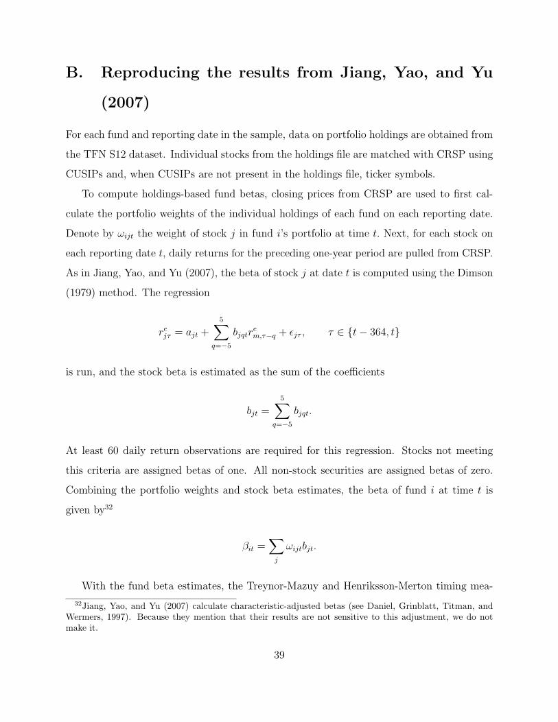
B. Reproducing the results from Jiang, Yao, and Yu

(2007)

For each fund and reporting date in the sample, data on portfolio holdings are obtained from

the TFN S12 dataset. Individual stocks from the holdings file are matched with CRSP using

CUSIPs and, when CUSIPs are not present in the holdings file, ticker symbols.

To compute holdings-based fund betas, closing prices from CRSP are used to first cal-

culate the portfolio weights of the individual holdings of each fund on each reporting date.

Denote by ωijt the weight of stock j in fund i’s portfolio at time t. Next, for each stock on

each reporting date t, daily returns for the preceding one-year period are pulled from CRSP.

As in Jiang, Yao, and Yu (2007), the beta of stock j at date t is computed using the Dimson

(1979) method. The regression

rejτ = ajt +5∑

q=−5

bjqtrem,τ−q + εjτ , τ ∈ {t− 364, t}

is run, and the stock beta is estimated as the sum of the coefficients

bjt =5∑

q=−5

bjqt.

At least 60 daily return observations are required for this regression. Stocks not meeting

this criteria are assigned betas of one. All non-stock securities are assigned betas of zero.

Combining the portfolio weights and stock beta estimates, the beta of fund i at time t is

given by32

βit =∑j

ωijtbjt.

With the fund beta estimates, the Treynor-Mazuy and Henriksson-Merton timing mea-

32Jiang, Yao, and Yu (2007) calculate characteristic-adjusted betas (see Daniel, Grinblatt, Titman, andWermers, 1997). Because they mention that their results are not sensitive to this adjustment, we do notmake it.

39

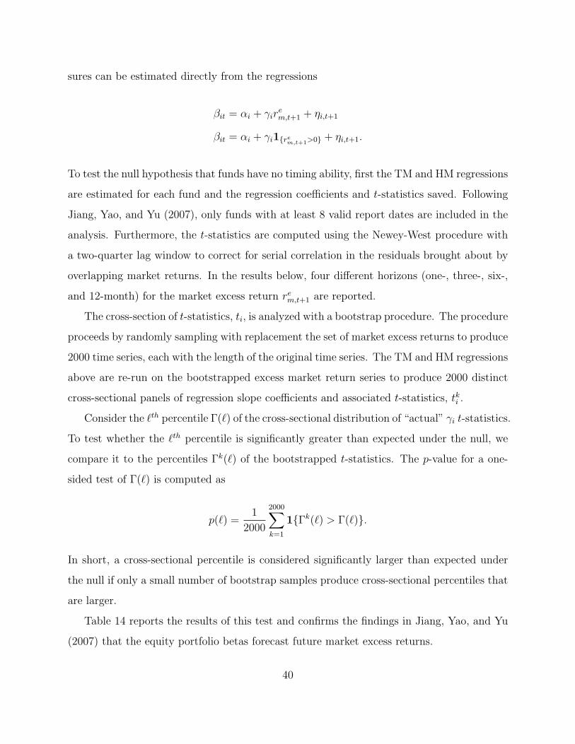
sures can be estimated directly from the regressions

βit = αi + γirem,t+1 + ηi,t+1

βit = αi + γi1{rem,t+1>0} + ηi,t+1.

To test the null hypothesis that funds have no timing ability, first the TM and HM regressions

are estimated for each fund and the regression coefficients and t-statistics saved. Following

Jiang, Yao, and Yu (2007), only funds with at least 8 valid report dates are included in the

analysis. Furthermore, the t-statistics are computed using the Newey-West procedure with

a two-quarter lag window to correct for serial correlation in the residuals brought about by

overlapping market returns. In the results below, four different horizons (one-, three-, six-,

and 12-month) for the market excess return rem,t+1 are reported.

The cross-section of t-statistics, ti, is analyzed with a bootstrap procedure. The procedure

proceeds by randomly sampling with replacement the set of market excess returns to produce

2000 time series, each with the length of the original time series. The TM and HM regressions

above are re-run on the bootstrapped excess market return series to produce 2000 distinct

cross-sectional panels of regression slope coefficients and associated t-statistics, tki .

Consider the `th percentile Γ(`) of the cross-sectional distribution of “actual” γi t-statistics.

To test whether the `th percentile is significantly greater than expected under the null, we

compare it to the percentiles Γk(`) of the bootstrapped t-statistics. The p-value for a one-

sided test of Γ(`) is computed as

p(`) =1

2000

2000∑k=1

1{Γk(`) > Γ(`)}.

In short, a cross-sectional percentile is considered significantly larger than expected under

the null if only a small number of bootstrap samples produce cross-sectional percentiles that

are larger.

Table 14 reports the results of this test and confirms the findings in Jiang, Yao, and Yu

(2007) that the equity portfolio betas forecast future market excess returns.

40

References

Almazan, A., K. C. Brown, M. Carlson, and D. A. Chapman, 2004, “Why Constrain your

Mutual Fund Manager?,” Journal of Financial Economics, 73(2), 289–321.

Austin, K., 1987, “Finite and Infinite Systems,” The Mathematical Gazette, 71(456), 107–

109.

Bollen, N. P. B., and J. A. Busse, 2001, “On the Timing Ability of Mutual Fund Managers,”

Journal of Finance, 56(3), 1075–1094.

Breen, W., L. R. Glosten, and R. Jagannathan, 1989, “Economic Significance of Predictable

Variations in Stock Index Returns,” Journal of Finance, 44(5), 1177–89.

Busse, J. A., 1999, “Volatility Timing in Mutual Funds: Evidence from Daily Returns,”

Review of Financial Studies, 12(5), 1009–41.

Campbell, J. Y., 2002, “Consumption-Based Asset Pricing,” Harvard Institute of Economic

Research Working Papers 1974, Harvard - Institute of Economic Research.

Campbell, J. Y., and R. J. Shiller, 1988a, “The Dividend-Price Ratio and Expectations of

Future Dividends and Discount Factors,” Review of Financial Studies, 1(3), 195–228.

Campbell, J. Y., and R. J. Shiller, 1988b, “Stock Prices, Earnings, and Expected Dividends,”

Journal of Finance, 43(3), 661–76.

Carhart, M. M., 1997, “On Persistence in Mutual Fund Performance,” Journal of Finance,

52(1), 57–82.

Chance, D. M., and M. L. Hemler, 2001, “The performance of professional market timers:

daily evidence from executed strategies,” Journal of Financial Economics, 62(2), 377–411.

Chen, H., N. Jegadeesh, and R. R. Wermers, 2000, “The Value of Active Mutual Fund Man-

agement: An Examination of the Stockholdings and Trades of Fund Managers,” Journal

of Financial and Quantitative Analysis, 35(3), 343–368.

41

Cohen, R. B., J. D. Coval, and L. Pastor, 2005, “Judging Fund Managers by the Company

They Keep,” Journal of Finance, 60(3), 1057–1096.

Cox, J. C., and H. E. Leland, 2000, “On dynamic investment strategies,” Journal of Eco-

nomic Dynamics and Control, 24(11-12), 1859–1880.

Daniel, K., M. Grinblatt, S. Titman, and R. Wermers, 1997, “Measuring Mutual Fund

Performance with Characteristic-Based Benchmarks,” Journal of Finance, 52(3), 1035–

58.

Davis, M.H.A., ., and A. R. Norman, 1990, “Portfolio selection with transaction costs,”

Mathematics of Operations Research, 15(4), 676–713.

Detemple, J. B., R. Garcia, and M. Rindisbacher, 2003, “A Monte Carlo Method for Optimal

Portfolios,” Journal of Finance, 58(1), 401–446.

Dimson, E., 1979, “Risk measurement when shares are subject to infrequent trading,” Jour-

nal of Financial Economics, 7(2), 197–226.

Edelen, R. M., 1999, “Investor flows and the assessed performance of open-end mutual

funds,” Journal of Financial Economics, 53(3), 439–466.

Edelen, R. M., and J. B. Warner, 2001, “Aggregate price effects of institutional trading: a

study of mutual fund flow and market returns,” Journal of Financial Economics, 59(2),

195–220.

Ferson, W. E., and R. W. Schadt, 1996, “Measuring Fund Strategy and Performance in

Changing Economic Conditions,” Journal of Finance, 51(2), 425–61.

Fleming, J., C. Kirby, and B. Ostdiek, 2001, “The economic value of volatility timing,”

Journal of Finance, 56(1), 329–352.

French, K. R., G. W. Schwert, and R. F. Stambaugh, 1987, “Expected stock returns and

volatility,” Journal of Financial Economics, 19(1), 3–29.

42

Goetzmann, W. N., J. Ingersoll, and Z. Ivkovic, 2000, “Monthly Measurement of Daily

Timers,” The Journal of Financial and Quantitative Analysis, 35(3), 257–290.

Graham, J. R., and C. R. Harvey, 1996, “Market timing ability and volatility implied in in-

vestment newsletters’ asset allocation recommendations,” Journal of Financial Economics,

42(3), 397–421.

Henriksson, R. D., and R. C. Merton, 1981, “On Market Timing and Investment Perfor-

mance. II. Statistical Procedures for Evaluating Forecasting Skills,” Journal of Business,

54(4), 513–33.

Jagannathan, R., and R. A. Korajczyk, 1986, “Assessing the Market Timing Performance

of Managed Portfolios,” Journal of Business, 59(2), 217–35.

Jiang, G. J., T. Yao, and T. Yu, 2007, “Do mutual funds time the market? Evidence from

portfolio holdings,” Journal of Financial Economics, 86, 724–758.

Kacperczyk, M., and A. Seru, 2007, “Fund Manager Use of Public Information: New Evi-

dence on Managerial Skills,” Journal of Finance, 62(2), 485–528.

Kacperczyk, M., C. Sialm, and L. Zheng, 2005, “On the Industry Concentration of Actively

Managed Equity Mutual Funds,” Journal of Finance, 60(4), 1983–2011.

Kandel, S., and R. F. Stambaugh, 1996, “On the Predictability of Stock Returns: An Asset-

Allocation Perspective,” Journal of Finance, 51(2), 385–424.

Keim, D. B., and R. F. Stambaugh, 1986, “Predicting returns in the stock and bond mar-

kets,” Journal of Financial Economics, 17(2), 357–390.

Kim, T. S., and E. Omberg, 1996, “Dynamic Nonmyopic Portfolio Behavior,” Review of

Financial Studies, 9(1), 141–61.

Kosowski, R., A. Timmermann, R. Wermers, and H. White, 2006, “Can Mutual Fund ”Stars”

Really Pick Stocks? New Evidence from a Bootstrap Analysis,” Journal of Finance, 61(6),

2551–2595.

43

Kothari, S., and J. Warner, 2001, “Evaluating Mutual Fund Performance,” Journal of Fi-

nance, 56(5), 1985–2010.

Kraus, A., and H. R. Stoll, 1972, “Parallel Trading by Institutional Investors,” The Journal

of Financial and Quantitative Analysis, 7(5), 2107–2138.

Leland, H. E., 1980, “Who Should Buy Portfolio Insurance?,” Journal of Finance, 35(2),

581–94.

Lettau, M., and S. Ludvigson, 2001, “Consumption, aggregate wealth and expected stock

returns,” Journal of Finance, 56, 815–849.

Pesaran, M. H., and A. G. Timmermann, 1994, “A generalization of the non-parametric

Henriksson-Merton test of market timing,” Economics Letters, 44(1-2), 1–7.

Treynor, J. L., and K. Mazuy, 1966, “Can mutual finds outguess the market?,” Harvard

Business Review, 44, 131–136.

Wachter, J. A., 2002, “Portfolio and Consumption Decisions under Mean-Reverting Returns:

An Exact Solution for Complete Markets,” Journal of Financial and Quantitative Analysis,

37(1), 63–91.

Wermers, R., 2000, “Mutual Fund Performance: An Empirical Decomposition into Stock-

Picking Talent, Style, Transactions Costs, and Expenses,” Journal of Finance, 55(4),

1655–1703.

White, H., 1980, “A Heteroskedasticity-Consistent Covariance Matrix Estimator and a Direct

Test for Heteroskedasticity,” Econometrica, 48(4), 817–38.

Whitelaw, R. F., 1994, “Time Variations and Covariations in the Expectation and Volatility

of Stock Market Returns,” Journal of Finance, 49(2), 515–41.

Whitelaw, R. F., 1997, “Time-Varying Sharpe Ratios and Market Timing,” New York Uni-

versity, Leonard N. Stern School Finance Department Working Paper Seires 98-074, New

York University, Leonard N. Stern School of Business-.

44

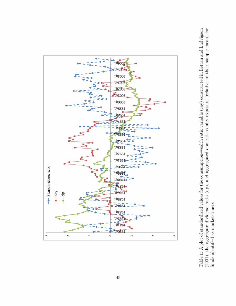
123Standardized

 wts

cay

dp

‐3‐2‐10

1980q1

1981q1

1982q1

1983q1

1984q1

1985q1

1986q1

1987q1

1988q1

1989q1

1990q1

1991q1

1992q1

1993q1

1994q1

1995q1

1996q1

1997q1

1998q1

1999q1

2000q1

2001q1

2002q1

2003q1

2004q1

2005q1

2006q1

Tab

le1:

Aplo

tof

stan

dar

diz

edva

lues

for

the

consu

mpti

on-w

ealt

hra

tio

vari

able

(cay

)co

nst

ruct

edin

Let

tau

and

Ludvig

son

(200

1),

the

aggr

egat

ediv

iden

dra

tio

(dp),

and

aggr

egat

eddom

esti

ceq

uit

yex

pos

ure

(rel

ativ

eto

thei

rsa

mple

mea

n)

for

funds

iden

tified

asm

arke

t-ti

mer

s

45

mod

al ioc

objective

Num

ber of fu

nds

1International

131

5Mun

iciple Bon

ds1

6Bo

nd & Preferred

18Metals

172Aggressive Growth

209

3Growth

1218

4Growth & Income

390

7Ba

lanced

147

9 or NAUnclassified

 or Unlisted

990ICDI objectiv

e code

ICDI objectiv

eNum

ber of fu

nds

150GB

Global Bon

d1

GE

Global Equ

ity8

IEInternational Equ

ity4

MF

Mon

ery Market M

uni

2SF

Sector Fun

d11

6UT

Utilities

3AG

Aggressive Growth

189

B LBa

lanced

8GI

Growth and

 Income

98IN

Income Fund

7LG

Long

‐term Growth

244

TRTo

tal Return Fund

5

CDA/Spe

ctrum s12

 objectiv

e

Total dropp

ed (shade

d)

551

1964

NA

Unclassified

 or un

listed

305S&

P ob

jective code

S&P ob

jective

Num

ber of fu

nds

134

NA

NA

9EG

GGlobal Equ

ity5

EGX

Global Equ

ity6

EIG

International Equ

ity0

FIN

Financial Sector

1HLT

Health

 Sector

9NTR

Natural Resou

rces

4RLE

Real Estate

10SEC

Sector Equ

ity3

TEC

Techno

log y

4UTI

Utilities

3AGG

Aggressive grow

th18

BAL

Balanced

5FLX

Asset Allocatio

n7

GMC

Midcap eq

uity

31GRI

Growth and

 Income

38GRO

Growth

82ING

Growth and

 Income

7SCG

Small‐cap

 Equ

ity63 54

Total dropp

ed (shade

d)

Total dropp

ed (shade

d)

251

Tab

le2:

This

table

dep

icts

the

obje

ctiv

escr

iter

iaw

euse

dfo

rse

lect

ing

funds

for

our

sam

ple

.F

unds

wer

efilt

ered

sequen

tial

lydep

endin

gon

the

avai

labilit

yof

obje

ctiv

esfr

omC

DA

/Sp

ectr

um

s12,

then

ICD

I,an

dth

enS&

P.

Funds

wit

hsh

aded

obje

ctiv

esw

ere

dro

pp

ed.

46

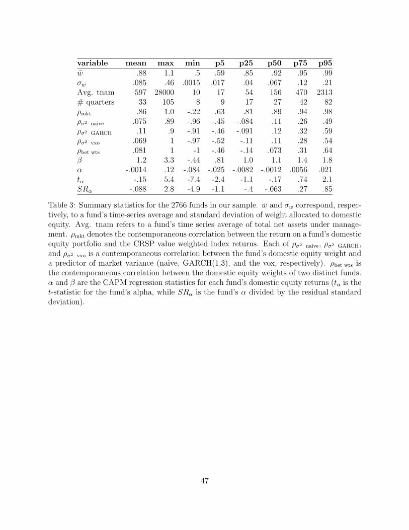
variable mean max min p5 p25 p50 p75 p95w .88 1.1 .5 .59 .85 .92 .95 .99σw .085 .46 .0015 .017 .04 .067 .12 .21Avg. tnam 597 28000 10 17 54 156 470 2313# quarters 33 105 8 9 17 27 42 82ρmkt .86 1.0 -.22 .63 .81 .89 .94 .98ρσ2 naive .075 .89 -.96 -.45 -.084 .11 .26 .49ρσ2 GARCH .11 .9 -.91 -.46 -.091 .12 .32 .59ρσ2 vxo .069 1 -.97 -.52 -.11 .11 .28 .54ρbet wts .081 1 -1 -.46 -.14 .073 .31 .64β 1.2 3.3 -.44 .81 1.0 1.1 1.4 1.8α -.0014 .12 -.084 -.025 -.0082 -.0012 .0056 .021tα -.15 5.4 -7.4 -2.4 -1.1 -.17 .74 2.1SRα -.088 2.8 -4.9 -1.1 -.4 -.063 .27 .85

Table 3: Summary statistics for the 2766 funds in our sample. w and σw correspond, respec-tively, to a fund’s time-series average and standard deviation of weight allocated to domesticequity. Avg. tnam refers to a fund’s time series average of total net assets under manage-ment. ρmkt denotes the contemporaneous correlation between the return on a fund’s domesticequity portfolio and the CRSP value weighted index returns. Each of ρσ2 naive, ρσ2 GARCH,and ρσ2 vxo is a contemporaneous correlation between the fund’s domestic equity weight anda predictor of market variance (naive, GARCH(1,3), and the vox, respectively). ρbet wts isthe contemporaneous correlation between the domestic equity weights of two distinct funds.α and β are the CAPM regression statistics for each fund’s domestic equity returns (tα is thet-statistic for the fund’s alpha, while SRα is the fund’s α divided by the residual standarddeviation).

47

Fund wficn code Fund name Fund wficn code Fund name100036 ADV FUND 102342 NORTHEAST INVTS GROWTH100150 AMANA MUTUAL FD-INCOME 102416 OPPENHEIMER DIRECTORS100189 PROVIDENT FD. FOR INCOME 102573 PHOENIX TOTAL RETURN100310 AVONDALE TOTAL RETURN FD 102734 PRUDENTIAL INST-ACT BAL100344 BEACON GROWTH FUND 102793 QUEST FOR VALUE/ASSET AL100358 ONE HUNDRED FUND 102979 SECURITY INVESTMENT FUND100359 BERGER 101 FUND 103045 SHEARSON L.STRATEGIC INV100473 CALVERT MANAGED GROWTH 103131 STAGECOACH LIFEPATH-2040100546 LOOMIS-SAYLES MUTUAL 103166 STEADMAN ASSOCIATED100743 DEAN WITTER STRATEGIST 103308 UNITED INCOME FUND100753 DECATUR INCOME FUND 103399 UNIFIED MUTUAL SHARES100879 ELFUN DIVERSIFIED 103415 UNITED CONTL. INCOME FD.101075 FIDELITY ASSET MGR-GRWTH 103418 UNITED FIDUCIARY SHARES101124 FIDUCIARY TOTAL RETURN 103491 VALUE LINE ASSET ALLOC101141 FINANCIAL INDUST. INCOME 103495 VALUE LINE INCOME101266 FOUNDERS EQUITY INCOME 103511 VANGUARD ASSET ALLOC FD101353 GALAXY ASSET ALLOCATION 105569 IDEX II TACT ASSET ALLOC101394 GENERAL SECURITIES 105629 SAND HILL PTF MGR FD101483 HAMILTON INCOME FUND 105810 LEONETTI BALANCED FUND101495 HANCOCK J SOVEREIGN BAL 105908 LEUTHOLD ASSET ALLOC FD101876 LEXINGTON RESEARCH FUND 107655 VANTAGEPOINT ASSET ALLOC101962 MAINSTAY TOTAL RETURN 109421 LORD ABBETT AMERICA’S VA102076 MERRILL LYNCH CAP FUND 240418 LINDBERGH SIGNATURE FUND102124 MUT.INV.FOUN.-MIF FUND 240436 MORGAN STANLEY ALLOCATOR102131 MIMLIC ASSET ALLOCATION 240438 ALPINE DYNAMIC BALANCE F102215 MUTUAL QUALIFIED INCOME 400220 AMERIPRIME IMS STRAT ALL102234 NATIONAL DIVIDEND 410127 MERRILL LYNCH BASIC VAL

Table 4: Fund names and wficn codes for the 54 funds we consider as ‘timers’.

48

variable mean max min p5 p25 p50 p75 p95w .69 .97 .51 .52 .6 .66 .77 .91σw .13 .26 .071 .074 .1 .13 .16 .25Avg. tnam 733 3991 11 13 64 242 886 3656# quarters 54 99 12 14 32 51 76 96ρmkt .91 .98 .77 .82 .88 .93 .95 .97ρσ2 naive .036 .57 -.9 -.28 -.12 .077 .23 .37ρσ2 GARCH 8.4e-04 .75 -.87 -.65 -.14 -.0077 .15 .53ρσ2 vxo .034 .65 -.96 -.38 -.11 .054 .24 .44ρbet wts .076 1 -.99 -.49 -.15 .072 .31 .64β 1.1 1.6 .88 .89 1 1.1 1.2 1.3α -2.3e-04 .023 -.015 -.0087 -.0039 -4.9e-04 .0031 .0088tα -.061 2.7 -3.1 -1.8 -.85 -.12 .49 2.3SRα -.054 .79 -1.2 -.72 -.23 -.033 .17 .51

Table 5: Summary statistics for the 54 ‘timers’ in our sample. w and σw correspond, respec-tively, to a fund’s time-series average and standard deviation of weight allocated to domesticequity. Avg. tnam refers to a fund’s time series average of total net assets under manage-ment. ρmkt denotes the contemporaneous correlation between the return on a fund’s domesticequity portfolio and the CRSP value weighted index returns. Each of ρσ2 naive, ρσ2 GARCH,and ρσ2 vxo is a contemporaneous correlation between the fund’s domestic equity weight anda predictor of market variance (naive, GARCH(1,3), and the vox, respectively). ρbet wts isthe contemporaneous correlation between the domestic equity weights of two distinct funds.α and β are the CAPM regression statistics for each fund’s domestic equity returns (tα is thet-statistic for the fund’s alpha, while SRα is the fund’s α divided by the residual standarddeviation).

49

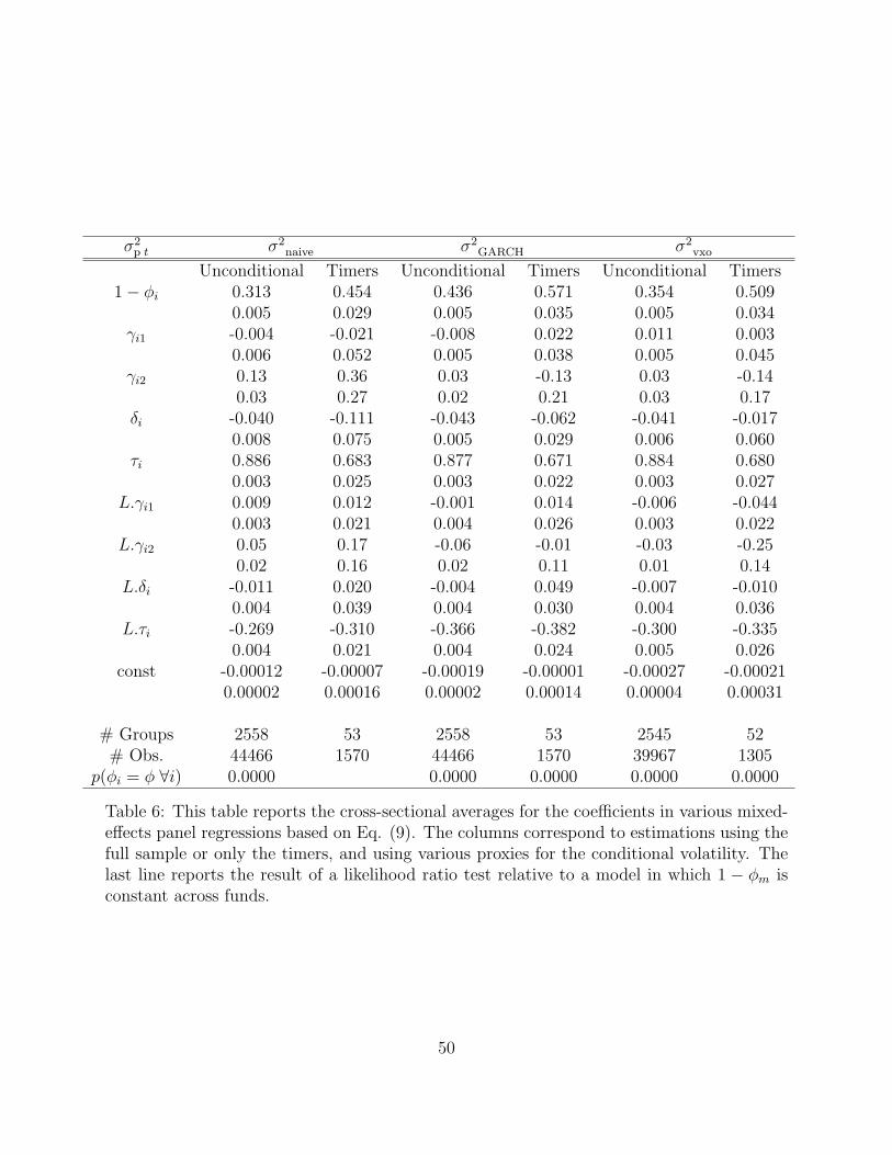
σ2p t σ2

naive σ2GARCH σ2

vxo

Unconditional Timers Unconditional Timers Unconditional Timers1− φi 0.313 0.454 0.436 0.571 0.354 0.509

0.005 0.029 0.005 0.035 0.005 0.034γi1 -0.004 -0.021 -0.008 0.022 0.011 0.003

0.006 0.052 0.005 0.038 0.005 0.045γi2 0.13 0.36 0.03 -0.13 0.03 -0.14

0.03 0.27 0.02 0.21 0.03 0.17δi -0.040 -0.111 -0.043 -0.062 -0.041 -0.017

0.008 0.075 0.005 0.029 0.006 0.060τi 0.886 0.683 0.877 0.671 0.884 0.680

0.003 0.025 0.003 0.022 0.003 0.027L.γi1 0.009 0.012 -0.001 0.014 -0.006 -0.044

0.003 0.021 0.004 0.026 0.003 0.022L.γi2 0.05 0.17 -0.06 -0.01 -0.03 -0.25

0.02 0.16 0.02 0.11 0.01 0.14L.δi -0.011 0.020 -0.004 0.049 -0.007 -0.010

0.004 0.039 0.004 0.030 0.004 0.036L.τi -0.269 -0.310 -0.366 -0.382 -0.300 -0.335

0.004 0.021 0.004 0.024 0.005 0.026const -0.00012 -0.00007 -0.00019 -0.00001 -0.00027 -0.00021

0.00002 0.00016 0.00002 0.00014 0.00004 0.00031

# Groups 2558 53 2558 53 2545 52# Obs. 44466 1570 44466 1570 39967 1305

p(φi = φ ∀i) 0.0000 0.0000 0.0000 0.0000 0.0000

Table 6: This table reports the cross-sectional averages for the coefficients in various mixed-effects panel regressions based on Eq. (9). The columns correspond to estimations using thefull sample or only the timers, and using various proxies for the conditional volatility. Thelast line reports the result of a likelihood ratio test relative to a model in which 1 − φm isconstant across funds.

50

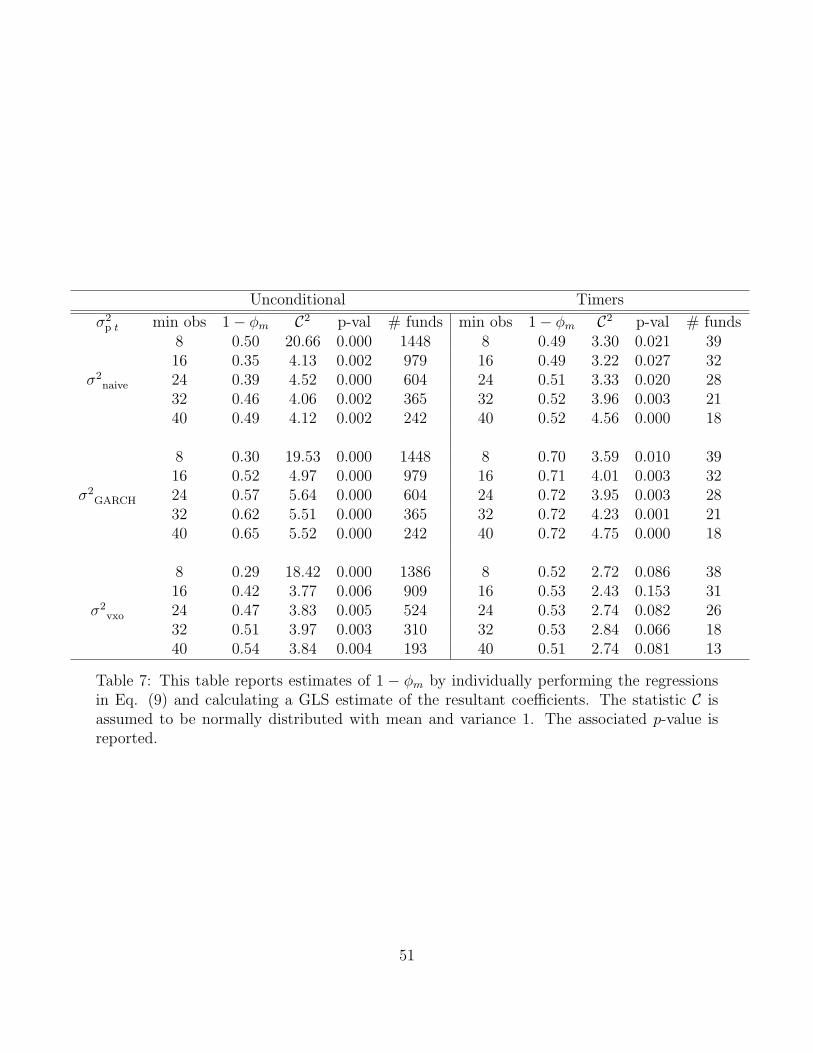
Unconditional Timers

σ2p t min obs 1− φm C2 p-val # funds min obs 1− φm C2 p-val # funds

σ2naive

8 0.50 20.66 0.000 1448 8 0.49 3.30 0.021 3916 0.35 4.13 0.002 979 16 0.49 3.22 0.027 3224 0.39 4.52 0.000 604 24 0.51 3.33 0.020 2832 0.46 4.06 0.002 365 32 0.52 3.96 0.003 2140 0.49 4.12 0.002 242 40 0.52 4.56 0.000 18

σ2GARCH

8 0.30 19.53 0.000 1448 8 0.70 3.59 0.010 3916 0.52 4.97 0.000 979 16 0.71 4.01 0.003 3224 0.57 5.64 0.000 604 24 0.72 3.95 0.003 2832 0.62 5.51 0.000 365 32 0.72 4.23 0.001 2140 0.65 5.52 0.000 242 40 0.72 4.75 0.000 18

σ2vxo

8 0.29 18.42 0.000 1386 8 0.52 2.72 0.086 3816 0.42 3.77 0.006 909 16 0.53 2.43 0.153 3124 0.47 3.83 0.005 524 24 0.53 2.74 0.082 2632 0.51 3.97 0.003 310 32 0.53 2.84 0.066 1840 0.54 3.84 0.004 193 40 0.51 2.74 0.081 13

Table 7: This table reports estimates of 1 − φm by individually performing the regressionsin Eq. (9) and calculating a GLS estimate of the resultant coefficients. The statistic C isassumed to be normally distributed with mean and variance 1. The associated p-value isreported.

51

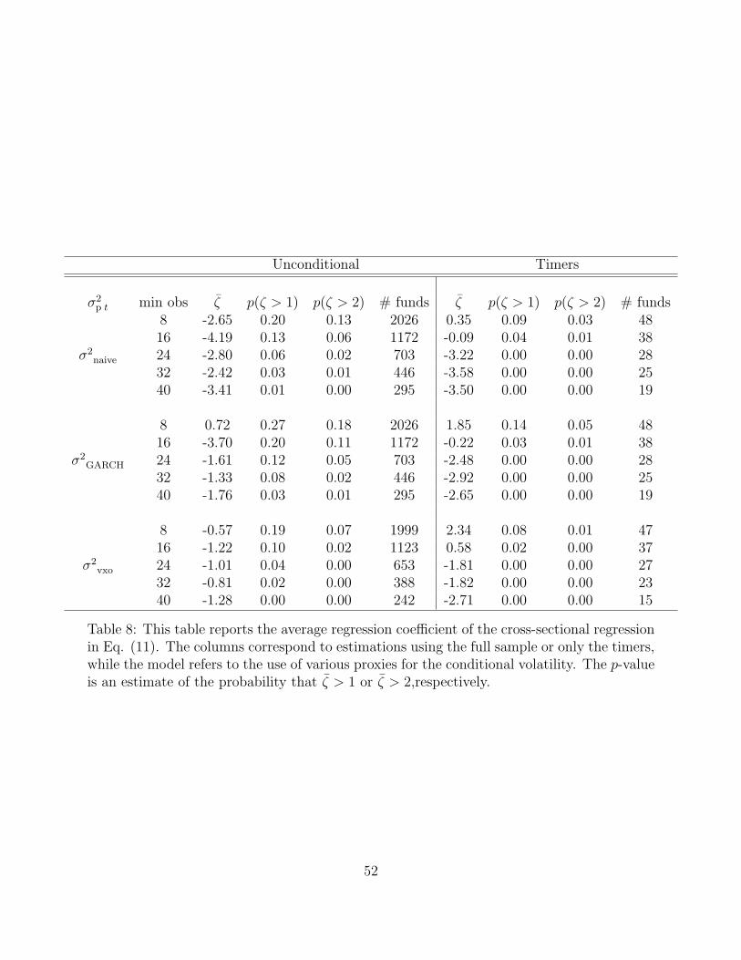
Unconditional Timers

σ2p t min obs ζ p(ζ > 1) p(ζ > 2) # funds ζ p(ζ > 1) p(ζ > 2) # funds

8 -2.65 0.20 0.13 2026 0.35 0.09 0.03 4816 -4.19 0.13 0.06 1172 -0.09 0.04 0.01 38

σ2naive 24 -2.80 0.06 0.02 703 -3.22 0.00 0.00 28

32 -2.42 0.03 0.01 446 -3.58 0.00 0.00 2540 -3.41 0.01 0.00 295 -3.50 0.00 0.00 19

8 0.72 0.27 0.18 2026 1.85 0.14 0.05 4816 -3.70 0.20 0.11 1172 -0.22 0.03 0.01 38

σ2GARCH 24 -1.61 0.12 0.05 703 -2.48 0.00 0.00 28

32 -1.33 0.08 0.02 446 -2.92 0.00 0.00 2540 -1.76 0.03 0.01 295 -2.65 0.00 0.00 19

8 -0.57 0.19 0.07 1999 2.34 0.08 0.01 4716 -1.22 0.10 0.02 1123 0.58 0.02 0.00 37

σ2vxo 24 -1.01 0.04 0.00 653 -1.81 0.00 0.00 27

32 -0.81 0.02 0.00 388 -1.82 0.00 0.00 2340 -1.28 0.00 0.00 242 -2.71 0.00 0.00 15

Table 8: This table reports the average regression coefficient of the cross-sectional regressionin Eq. (11). The columns correspond to estimations using the full sample or only the timers,while the model refers to the use of various proxies for the conditional volatility. The p-valueis an estimate of the probability that ζ > 1 or ζ > 2,respectively.

52

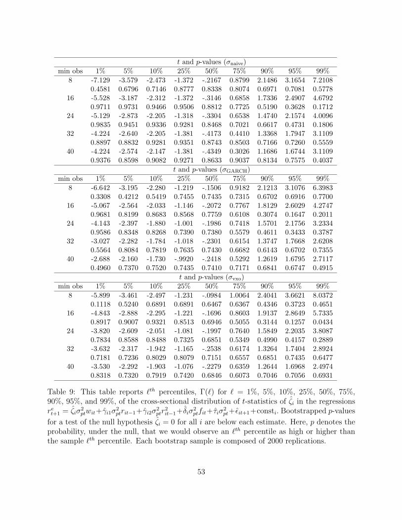
t and p-values (σnaive)min obs 1% 5% 10% 25% 50% 75% 90% 95% 99%

8 -7.129 -3.579 -2.473 -1.372 -.2167 0.8799 2.1486 3.1654 7.21080.4581 0.6796 0.7146 0.8777 0.8338 0.8074 0.6971 0.7081 0.5778

16 -5.528 -3.187 -2.312 -1.372 -.3146 0.6858 1.7336 2.4907 4.67920.9711 0.9731 0.9466 0.9506 0.8812 0.7725 0.5190 0.3628 0.1712

24 -5.129 -2.873 -2.205 -1.318 -.3304 0.6538 1.4740 2.1574 4.00960.9835 0.9451 0.9336 0.9281 0.8468 0.7021 0.6617 0.4731 0.1806

32 -4.224 -2.640 -2.205 -1.381 -.4173 0.4410 1.3368 1.7947 3.11090.8897 0.8832 0.9281 0.9351 0.8743 0.8503 0.7166 0.7260 0.5559

40 -4.224 -2.574 -2.147 -1.381 -.4349 0.3026 1.1686 1.6744 3.11090.9376 0.8598 0.9082 0.9271 0.8633 0.9037 0.8134 0.7575 0.4037

t and p-values (σGARCH)min obs 1% 5% 10% 25% 50% 75% 90% 95% 99%

8 -6.642 -3.195 -2.280 -1.219 -.1506 0.9182 2.1213 3.1076 6.39830.3308 0.4212 0.5419 0.7455 0.7435 0.7315 0.6702 0.6916 0.7700

16 -5.067 -2.564 -2.033 -1.146 -.2072 0.7767 1.8129 2.6029 4.27470.9681 0.8199 0.8683 0.8568 0.7759 0.6108 0.3074 0.1647 0.2011

24 -4.143 -2.397 -1.880 -1.001 -.1986 0.7418 1.5701 2.1756 3.23340.9586 0.8348 0.8268 0.7390 0.7380 0.5579 0.4611 0.3433 0.3787

32 -3.027 -2.282 -1.784 -1.018 -.2301 0.6154 1.3747 1.7668 2.62080.5564 0.8084 0.7819 0.7635 0.7430 0.6682 0.6143 0.6702 0.7355

40 -2.688 -2.160 -1.730 -.9920 -.2418 0.5292 1.2619 1.6795 2.71170.4960 0.7370 0.7520 0.7435 0.7410 0.7171 0.6841 0.6747 0.4915

t and p-values (σvxo)min obs 1% 5% 10% 25% 50% 75% 90% 95% 99%

8 -5.899 -3.461 -2.497 -1.231 -.0984 1.0064 2.4041 3.6621 8.03720.1118 0.5240 0.6891 0.6891 0.6467 0.6367 0.4346 0.3723 0.4651

16 -4.843 -2.888 -2.295 -1.221 -.1696 0.8603 1.9137 2.8649 5.73350.8917 0.9007 0.9321 0.8513 0.6946 0.5055 0.3144 0.1257 0.0434

24 -3.820 -2.609 -2.051 -1.081 -.1997 0.7640 1.5849 2.2035 3.80870.7834 0.8588 0.8488 0.7325 0.6851 0.5349 0.4990 0.4157 0.2889

32 -3.632 -2.317 -1.942 -1.165 -.2538 0.6174 1.3264 1.7404 2.89240.7181 0.7236 0.8029 0.8079 0.7151 0.6557 0.6851 0.7435 0.6477

40 -3.530 -2.292 -1.903 -1.076 -.2279 0.6359 1.2644 1.6968 2.49740.8318 0.7320 0.7919 0.7420 0.6846 0.6073 0.7046 0.7056 0.6931

Table 9: This table reports `th percentiles, Γ(`) for ` = 1%, 5%, 10%, 25%, 50%, 75%,90%, 95%, and 99%, of the cross-sectional distribution of t-statistics of ζi in the regressionsret+1 = ζiσ

2ptwit+γi1σ

2ptrit−1+γi2σ

2ptr

2it−1+δiσ

2ptfit+τiσ

2pt+ εit+1+consti. Bootstrapped p-values

for a test of the null hypothesis ζi = 0 for all i are below each estimate. Here, p denotes theprobability, under the null, that we would observe an `th percentile as high or higher thanthe sample `th percentile. Each bootstrap sample is composed of 2000 replications.

53

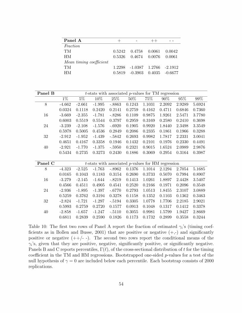
Panel A + - ++ - -FractionTM 0.5242 0.4758 0.0061 0.0042HM 0.5326 0.4674 0.0076 0.0061Mean timing coefficientTM 1.2298 -1.0387 1.2766 -2.1912HM 0.5819 -0.3903 0.4035 -0.6677

Panel B t-stats with associated p-values for TM regression1% 5% 10% 25% 50% 75% 90% 95% 99%

8 -4.662 -2.661 -1.995 -.8863 0.1243 1.1031 2.2092 2.9289 5.69240.0324 0.1118 0.2420 0.2141 0.2759 0.4162 0.4711 0.6846 0.7360

16 -3.669 -2.355 -1.781 -.8286 0.1109 0.9875 1.9261 2.5471 3.77800.6003 0.5519 0.5544 0.3797 0.2959 0.3169 0.2580 0.2410 0.3698

24 -3.239 -2.108 -1.576 -.6920 0.1905 0.9920 1.8440 2.3498 3.35490.5978 0.5005 0.4536 0.2849 0.2086 0.2335 0.1861 0.1966 0.3288

32 -2.912 -1.952 -1.439 -.5842 0.2693 0.9982 1.7817 2.2331 3.00410.4651 0.4167 0.3358 0.1946 0.1432 0.2101 0.1976 0.2330 0.4491

40 -2.921 -1.770 -1.375 -.5950 0.2321 0.9015 1.6524 2.0989 2.98760.5434 0.2735 0.3273 0.2430 0.1886 0.3069 0.2954 0.3164 0.3987

Panel C t-stats with associated p-values for HM regression8 -4.323 -2.525 -1.763 -.8962 0.1376 1.1014 2.1294 2.7054 5.1685

0.0165 0.1043 0.1183 0.3154 0.2690 0.3733 0.5070 0.7994 0.890716 -3.279 -2.145 -1.644 -.8219 0.1413 1.0261 1.8897 2.4428 3.5407

0.4566 0.4511 0.4905 0.4541 0.2520 0.2166 0.1971 0.2096 0.354824 -2.936 -1.895 -1.397 -.6770 0.2793 1.0513 1.8455 2.3107 3.0889

0.5259 0.3762 0.3194 0.3278 0.1158 0.1352 0.1103 0.1362 0.346332 -2.824 -1.721 -1.297 -.5194 0.3305 1.0778 1.7706 2.2185 2.9021

0.5993 0.2759 0.2720 0.1577 0.0913 0.1048 0.1317 0.1412 0.337840 -2.858 -1.657 -1.247 -.5110 0.3055 0.9981 1.5799 1.9427 2.8669

0.6811 0.2839 0.2590 0.1826 0.1173 0.1732 0.2899 0.3558 0.3244

Table 10: The first two rows of Panel A report the fraction of estimated γi’s (timing coef-ficients as in Bollen and Busse, 2001) that are positive or negative (+,-) and significantlypositive or negative (++/- -). The second two rows report the conditional means of theγi’s, given that they are positive, negative, significantly positive, or significantly negative.Panels B and C reports percentiles, Γ(`), of the cross-sectional distribution of t for the timingcoefficient in the TM and HM regressions. Bootstrapped one-sided p-values for a test of thenull hypothesis of γ = 0 are included below each percentile. Each bootstrap consists of 2000replications.

54

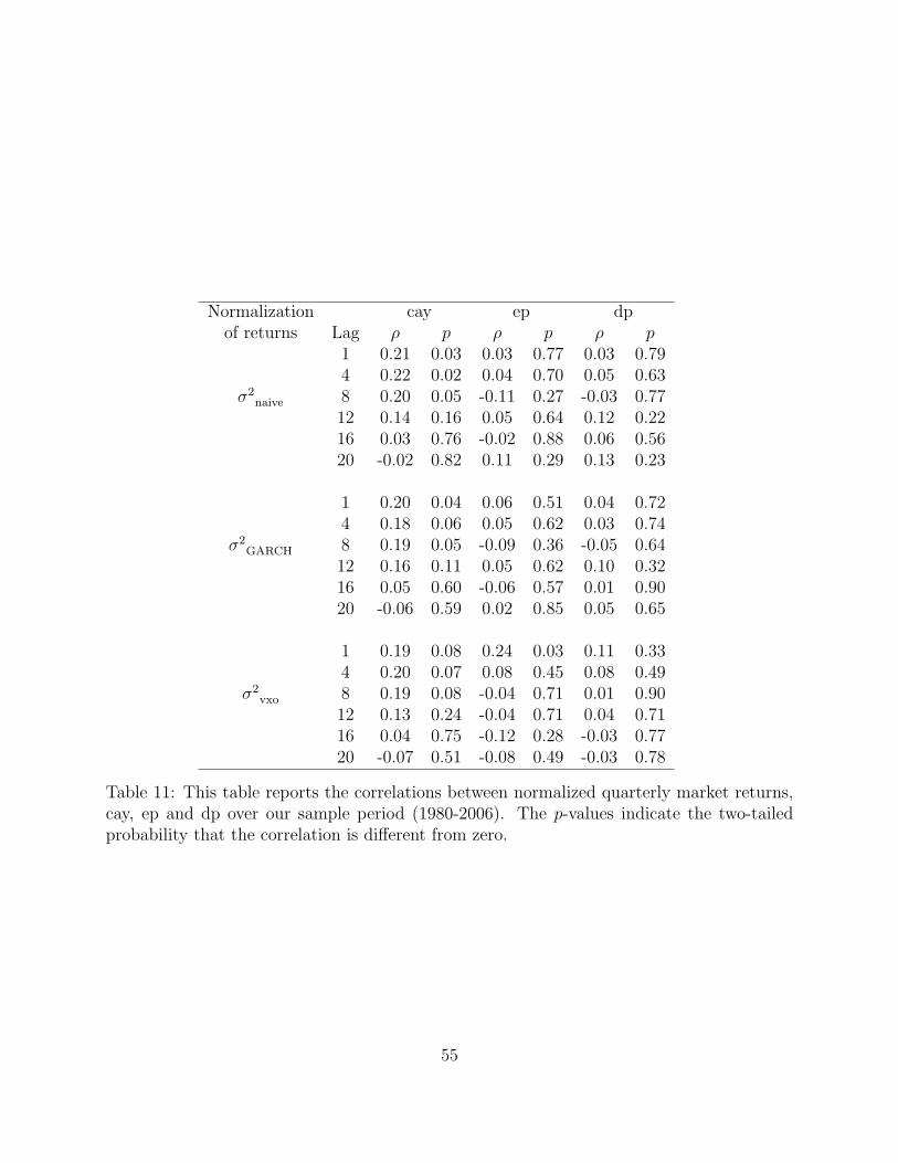
Normalization cay ep dpof returns Lag ρ p ρ p ρ p

1 0.21 0.03 0.03 0.77 0.03 0.794 0.22 0.02 0.04 0.70 0.05 0.63

σ2naive 8 0.20 0.05 -0.11 0.27 -0.03 0.77

12 0.14 0.16 0.05 0.64 0.12 0.2216 0.03 0.76 -0.02 0.88 0.06 0.5620 -0.02 0.82 0.11 0.29 0.13 0.23

1 0.20 0.04 0.06 0.51 0.04 0.724 0.18 0.06 0.05 0.62 0.03 0.74

σ2GARCH 8 0.19 0.05 -0.09 0.36 -0.05 0.64

12 0.16 0.11 0.05 0.62 0.10 0.3216 0.05 0.60 -0.06 0.57 0.01 0.9020 -0.06 0.59 0.02 0.85 0.05 0.65

1 0.19 0.08 0.24 0.03 0.11 0.334 0.20 0.07 0.08 0.45 0.08 0.49

σ2vxo 8 0.19 0.08 -0.04 0.71 0.01 0.90

12 0.13 0.24 -0.04 0.71 0.04 0.7116 0.04 0.75 -0.12 0.28 -0.03 0.7720 -0.07 0.51 -0.08 0.49 -0.03 0.78

Table 11: This table reports the correlations between normalized quarterly market returns,cay, ep and dp over our sample period (1980-2006). The p-values indicate the two-tailedprobability that the correlation is different from zero.

55

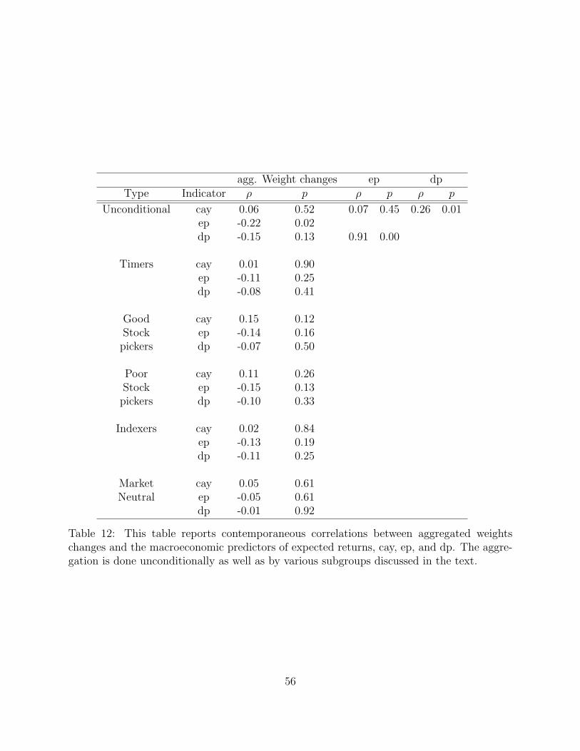
agg. Weight changes ep dpType Indicator ρ p ρ p ρ p

Unconditional cay 0.06 0.52 0.07 0.45 0.26 0.01ep -0.22 0.02dp -0.15 0.13 0.91 0.00

Timers cay 0.01 0.90ep -0.11 0.25dp -0.08 0.41

Good cay 0.15 0.12Stock ep -0.14 0.16

pickers dp -0.07 0.50

Poor cay 0.11 0.26Stock ep -0.15 0.13

pickers dp -0.10 0.33

Indexers cay 0.02 0.84ep -0.13 0.19dp -0.11 0.25

Market cay 0.05 0.61Neutral ep -0.05 0.61

dp -0.01 0.92

Table 12: This table reports contemporaneous correlations between aggregated weightschanges and the macroeconomic predictors of expected returns, cay, ep, and dp. The aggre-gation is done unconditionally as well as by various subgroups discussed in the text.

56

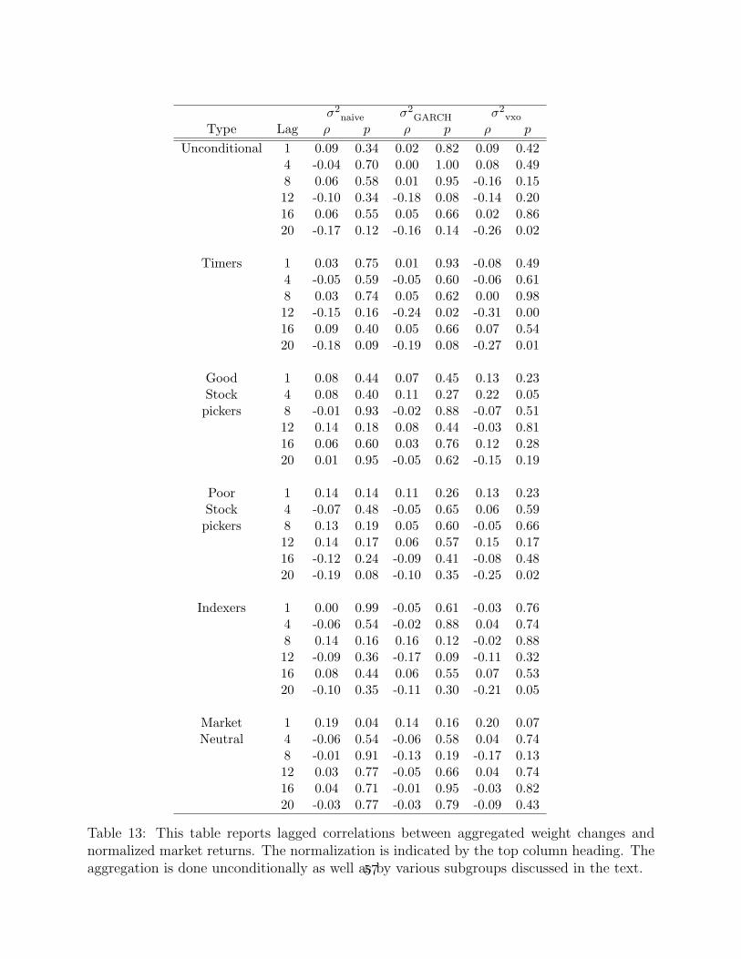
σ2naive σ2

GARCH σ2vxo

Type Lag ρ p ρ p ρ p

Unconditional 1 0.09 0.34 0.02 0.82 0.09 0.424 -0.04 0.70 0.00 1.00 0.08 0.498 0.06 0.58 0.01 0.95 -0.16 0.1512 -0.10 0.34 -0.18 0.08 -0.14 0.2016 0.06 0.55 0.05 0.66 0.02 0.8620 -0.17 0.12 -0.16 0.14 -0.26 0.02

Timers 1 0.03 0.75 0.01 0.93 -0.08 0.494 -0.05 0.59 -0.05 0.60 -0.06 0.618 0.03 0.74 0.05 0.62 0.00 0.9812 -0.15 0.16 -0.24 0.02 -0.31 0.0016 0.09 0.40 0.05 0.66 0.07 0.5420 -0.18 0.09 -0.19 0.08 -0.27 0.01

Good 1 0.08 0.44 0.07 0.45 0.13 0.23Stock 4 0.08 0.40 0.11 0.27 0.22 0.05

pickers 8 -0.01 0.93 -0.02 0.88 -0.07 0.5112 0.14 0.18 0.08 0.44 -0.03 0.8116 0.06 0.60 0.03 0.76 0.12 0.2820 0.01 0.95 -0.05 0.62 -0.15 0.19

Poor 1 0.14 0.14 0.11 0.26 0.13 0.23Stock 4 -0.07 0.48 -0.05 0.65 0.06 0.59

pickers 8 0.13 0.19 0.05 0.60 -0.05 0.6612 0.14 0.17 0.06 0.57 0.15 0.1716 -0.12 0.24 -0.09 0.41 -0.08 0.4820 -0.19 0.08 -0.10 0.35 -0.25 0.02

Indexers 1 0.00 0.99 -0.05 0.61 -0.03 0.764 -0.06 0.54 -0.02 0.88 0.04 0.748 0.14 0.16 0.16 0.12 -0.02 0.8812 -0.09 0.36 -0.17 0.09 -0.11 0.3216 0.08 0.44 0.06 0.55 0.07 0.5320 -0.10 0.35 -0.11 0.30 -0.21 0.05

Market 1 0.19 0.04 0.14 0.16 0.20 0.07Neutral 4 -0.06 0.54 -0.06 0.58 0.04 0.74

8 -0.01 0.91 -0.13 0.19 -0.17 0.1312 0.03 0.77 -0.05 0.66 0.04 0.7416 0.04 0.71 -0.01 0.95 -0.03 0.8220 -0.03 0.77 -0.03 0.79 -0.09 0.43

Table 13: This table reports lagged correlations between aggregated weight changes andnormalized market returns. The normalization is indicated by the top column heading. Theaggregation is done unconditionally as well as by various subgroups discussed in the text.57

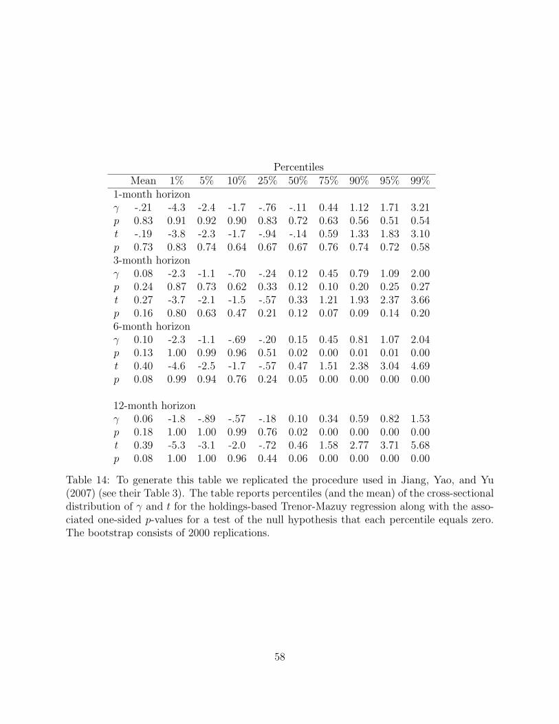
PercentilesMean 1% 5% 10% 25% 50% 75% 90% 95% 99%

1-month horizonγ -.21 -4.3 -2.4 -1.7 -.76 -.11 0.44 1.12 1.71 3.21p 0.83 0.91 0.92 0.90 0.83 0.72 0.63 0.56 0.51 0.54t -.19 -3.8 -2.3 -1.7 -.94 -.14 0.59 1.33 1.83 3.10p 0.73 0.83 0.74 0.64 0.67 0.67 0.76 0.74 0.72 0.583-month horizonγ 0.08 -2.3 -1.1 -.70 -.24 0.12 0.45 0.79 1.09 2.00p 0.24 0.87 0.73 0.62 0.33 0.12 0.10 0.20 0.25 0.27t 0.27 -3.7 -2.1 -1.5 -.57 0.33 1.21 1.93 2.37 3.66p 0.16 0.80 0.63 0.47 0.21 0.12 0.07 0.09 0.14 0.206-month horizonγ 0.10 -2.3 -1.1 -.69 -.20 0.15 0.45 0.81 1.07 2.04p 0.13 1.00 0.99 0.96 0.51 0.02 0.00 0.01 0.01 0.00t 0.40 -4.6 -2.5 -1.7 -.57 0.47 1.51 2.38 3.04 4.69p 0.08 0.99 0.94 0.76 0.24 0.05 0.00 0.00 0.00 0.00

12-month horizonγ 0.06 -1.8 -.89 -.57 -.18 0.10 0.34 0.59 0.82 1.53p 0.18 1.00 1.00 0.99 0.76 0.02 0.00 0.00 0.00 0.00t 0.39 -5.3 -3.1 -2.0 -.72 0.46 1.58 2.77 3.71 5.68p 0.08 1.00 1.00 0.96 0.44 0.06 0.00 0.00 0.00 0.00

Table 14: To generate this table we replicated the procedure used in Jiang, Yao, and Yu(2007) (see their Table 3). The table reports percentiles (and the mean) of the cross-sectionaldistribution of γ and t for the holdings-based Trenor-Mazuy regression along with the asso-ciated one-sided p-values for a test of the null hypothesis that each percentile equals zero.The bootstrap consists of 2000 replications.

58